Attenuation and Velocity Structure for Site Response Analyses via

Downhole Seismogram Inversion

DOMINIC ASSIMAKI,1 JAMISON STEIDL,2 and PENG CHENG LIU2

Abstract—A seismic waveform inversion algorithm is proposed for the estimation of elastic soil

properties using low amplitude, downhole array recordings. Based on a global optimization scheme in

the wavelet domain, complemented by a local least-square’s fit operator in the frequency domain, the

hybrid scheme can efficiently identify the optimal solution vicinity in the stochastic search space, whereas

the best-fit model detection is substantially accelerated through the local deterministic inversion. Results

presented for selected aftershocks of the Mw 7.0 Sanriku-Minami earthquake in Japan, recorded by the

Kik-Net Strong Motion Network, illustrate robustness of the impedance structure estimation. By

contrast, the attenuation structure is shown to be sensitive to the frequency content of seismic input

data, attributed to the deterministic description of the continuum in the forward model that cannot

simulate late arrivals of multiple-scattered energy. Sensitivity analyses illustrate that for the same

forward model, results can be substantially different based on the definition of the objective function. It

is concluded that even for engineering purposes, inversion should aim to decouple intrinsic and

scattering attenuation mechanisms.

Key words: Seismogram inversion, genetic algorithms, site response, Scattering attenuation.

1. Introduction

It has been long recognized that the destructiveness of ground shaking during

earthquakes can be significantly enhanced by local soil conditions, a term that refers to

the mechanical properties of the surficial geological formations. Thus, during past

events, the observed variability in seismic intensity and structural damage severity has

been often attributed to the variability of soil stratigraphy at a given area. Examples

include—among others—the non-uniform distribution of damage in Tokyo during

the 1923 Kanto Earthquake (OHSAKI, 1969); in Caracas during the 1967 Venezuelan

Earthquake (SEED et al., 1972); in Bucharest during the 1977 Vranehla Earthquake

(TEZCAN et al., 1979); in Mexico City during the Earthquakes of 1957 and especially

of 1985 (ROSENBLUETH, 1960; SEED and ROMO, 1987); in San Francisco and Oakland

1School of Civil and Environmental Engineering, Georgia Institute of Technology, 790, AtlanticDrive, Atlanta, GA 30332, U.S.A. E-mail: dassimak@mit.edu

2Institute for Crustal Studies, University of California, 1140 Girvetz Hall, Santa Barbara, CA 93106,U.S.A. E-mail: steidl@crustal.ucsb.edu E-mail: pcliu@crustal.ucsb.edu

Pure appl. geophys. 163 (2006) 81–1180033–4553/06/010081–38DOI 10.1007/s00024-005-0009-7

� Birkhauser Verlag, Basel, 2006

Pure and Applied Geophysics

during the 1989 Loma Prieta Earthquake (HOUSNER, 1990); in Kobe during the 1995

Earthquake (special issue of SOIL and FOUNDATIONS, 1996); and in Adapazari during

the Kocaeli Earthquake (special issue of EARTHQUAKE SPECTRA, 2000).

Observations of ground motion recorded in the last three decades reveal in many

cases that subsoil characteristics had significant influence on the amplitude level,

frequency composition, and duration of surface ground shaking. Therefore, the

detailed description of local soil conditions at any site, is critical for the assessment of

seismic risk, for microzonation studies and for the seismic design and retrofit of

important facilities and long structures.

In site response assessment methodologies, elastic simulations primarily rely on

geotechnical and geophysical testing procedures to provide the necessary information

on density and low-strain shear-wave velocity variation with depth. Even further,

attenuation, a critical yet least explored mechanism of seismic energy dissipation and

redistribution, is either approximated by means of empirical correlations or inferred

based on limited laboratory data. At larger strains, which the material is anticipated

to experience during strong motion events, soil properties are mainly evaluated

through laboratory testing. Nonetheless, even the applicability of laboratory testing

is limited, due to sample disturbance and difficulties in reproducing the in situ stress-

state and seismic loading.

The scarcity of near-surface geotechnical information, error propagation of

laboratory and in situ measurement techniques, and limited resolution of the

continuum, usually result in predictions of surface ground motion that poorly

compare with low amplitude observations. This discrepancy is even further

aggravated for strong ground motion, associated with hysteretic, nonlinear, and

potentially irreversible material deformations.

Seismic observations of site response may be a valuable complement to in situ and

laboratory geotechnical investigation techniques. Downhole instrumentation in

particular, has been increasingly deployed in seismically active areas over the past

years (e.g., Japan, United States, Taiwan, Mexico, Greece), providing critical

constraints on interpretation methods for surface observations, as well as informa-

tion on the real material behavior and overall site response over a wide range of

loading conditions. For example, borehole measurements provided direct in situ

evidence of nonlinearity (e.g., SEED and IDRISS, 1970; WEN et al., 1994; ZEGHAL and

ELGAMAL, 1994; IAI et al., 1995; SATO et al., 1996; AGUIRRE and IRIKURA, 1997;

SATOH et al., 2001); they have invited a re-evaluation of the use of surface-rock

recordings as input motion to soil columns (e.g. SATOH et al., 1995; STEIDL et al.,

1996; BOORE and JOYNER, 1997), and they have provided basic information about

scaling properties of the spectra of earthquakes of different magnitudes (e.g.,

KINOSHITA, 1992; ABERCROMBIE, 1997).

In this study, a seismic waveform inversion algorithm is proposed for the

estimation of elastic soil properties using low amplitude, downhole array recordings.

Based on a global optimization scheme complemented by a local least-squares fit

82 D. Assimaki et al. Pure appl. geophys.,

operator, the proposed algorithm is shown to estimate efficiently the soil shear-wave

velocity, attenuation and density variation with depth.

2. Inversion of the Elastic Soil Structure

Seismogram inversion is a nonlinear multi-parametric problem, where one

attempts to estimate physical parameters from available data. In ideal cases, there

exists an exact theory that prescribes how the data should be transformed to

reconstruct the model, usually provided that infinitely many and noise-free data sets

are available. Therefore, despite the mathematical elegance of exact nonlinear

inversion schemes, they have the following drawbacks: (i) they are applicable to ideal

conditions, (ii) they are often unstable, and (iii) they usually predict continuous

functions of space variables based on a finite number of available data.

The fact that in realistic experiments, a finite amount of data is available to

reconstruct a model with infinitely many degrees of freedom, necessarily implies that

the inverse problem is not unique, namely there exist several (usually infinitely many)

models that explain the data equally well. Clearly, in this case, the model estimated

by means of data inversion is not necessarily equal to the true model, and the

inversion process needs also to appraise what properties of the true model are

recovered by the best-fit model, and what errors are attached to it; in fact,

acknowledging the existence of errors and limited resolution is necessary for the

physical interpretation of a model (SNIEDER and TRAMPERT, 1999; TRAMPERT, 1998).

Nonlinearity introduces additional complexity to the inverse analysis, affecting

both the estimation and the appraisal problem, and—in practical problems—it is

usually treated as a nonlinear optimization problem, where a suitably chosen

measure of the data misfit is reduced as a function of the model parameters.

In seismic applications, two data misfit measures are commonly used. One is the

error defined as E(m)=d)g(m), where m and d are model and data vectors

respectively, and g is the forward modeling operator. The optimization process

determines the m’s that minimize the error energy. A second measure is the

normalized correlation function, defined as follows:

CðmÞ ¼ d� gðmÞðd� dÞ1=2ðgðmÞ � gðmÞÞ1=2

; ð1Þ

where � represents the cross-correlation; in this case, the optimization scheme

estimates the m’s that maximize C(m). Both these functions are referred to as

‘‘objective’’ or ‘‘fitness’’ functions.

In the forward problem, the model parameters are nonlinearly related to the

measured process, reflected on C(m) and E(m) as multiple local maxima and minima,

respectively. As a result, traditional search techniques based on local linearization,

which use characteristics of the problem to determine the next sampling point (e.g.,

Vol. 163, 2006 A Seismic Waveform Inversion Algorithm 83

gradients, Hessians, linearity and continuity) are computationally efficient, but fail to

identify the best-fit solution, when the starting model is too far from the global

optimal solution. On the other hand, stochastic search techniques (e.g., genetic

algorithms, simulated annealing) have been shown to efficiently identify promising

regions in the search space, but perform very poorly in a localized search (DAVIS,

1991; MICHALEWICZ, 1994; BERSINI and RENDERS, 1994; HOUCK et al., 1996).

The proposed optimization technique is a two-step process, namely a genetic

algorithm in the wavelet domain coupled to a nonlinear least-squares fit in the

frequency domain; we thus improve the computational efficiency of the former, while

avoiding the pitfalls of using local linearization techniques—such as the latter—for

the optimization of multi-modal, discontinuous and non-differentiable functions.

The parameters to be estimated are stepwise variations of the shear-wave velocity,

attenuation and density with depth, for horizontally layered media with predefined

layer thickness. Equality constrains are imposed on the vector of unknowns to bound

the search space, based on independent geological and geotechnical site character-

ization data. Note that for the discretization of the continuum, a preliminary analysis

precedes the inversion process to ensure that the layer thicknesses are at least equal to

the quarter-length of propagating waveforms (hi ‡ Vsi / 4fmax); the satisfaction of this

criterion is also verified at convergence of the optimization algorithm.

2.1 Numerical Simulation and Data Processing

One-dimensional downhole seismograms can be simulated by means of standard

frequency domain analyses, as proposed by BRUNE (1970) and revised by MADAR-

IAGA (1976). Accounting both for upgoing and downgoing waves, we here use the

HASKELL-THOMPSON (1978) transfer function for horizontally layered media over-

lying rigid bedrock and subjected to anti-plane (SH) incident motion. In this

representation, each layer of soil behaves as a Kelvin-Voigt solid.

The forward model schematically illustrated in Figure 1, comprises n homoge-

neous, horizontal soil layers overlying bedrock, where the total motion is prescribed

and equal to uR. The soil layers have the following characteristics:

hi; qi; Vsi ; Qi; i ¼ 1; 2; . . . N ; ð2Þ

where: h = thickness [m], q= density [Mg/m3], Vs = shear-wave velocity [m/sec],

and 1/2Q = hysteretic damping.

At any given layer, i, at a given input frequency, f, we consider the following

complex quantities:

V �si¼ Vsi

ffiffiffiffiffiffiffiffiffiffiffiffiffi

1þ iQi

s

G�i ¼ qiV2

si1þ i

Qi

� �

k�i ¼x

Vsi

ffiffiffiffiffiffiffiffiffiffiffiffi

1þ iQi

q ¼ 2pf

Vsi

ffiffiffiffiffiffiffiffiffiffiffiffi

1þ iQi

q ; ð3Þ

where: V �siis the complex shear-wave velocity, G�i is the complex shear modulus, and

k�i is the complex wavenumber.

84 D. Assimaki et al. Pure appl. geophys.,

We also define: (i) z = 0.0 at the free surface (stress-free boundary) of the profile,

(ii) zi ¼P

i

j¼1hi as the total depth of the ith layer, (iii) Ai as the amplitude of the

downgoing waves at each layer, and (iv) Bi as the amplitude of upgoing waves at each

layer.

The total motion in each layer (summation of upgoing and downgoing waves) is:

ui ¼ Aieiðxtþk�i ziÞ þ Bieiðxt�k�i ziÞ ð4Þ

Therefore, the total shear stress in each layer is defined as:

si ¼ ik�i G�i Aieiðxtþk�i ziÞ � ik�i G�i Bieiðxt�k�i ziÞ: ð5Þ

We now define the matrix of displacement-stress coefficients as follows:

ui

si

� �

¼ eik�i zi e�ik�i zi

ik�i G�i eik�i zi �ik�i G�i eik�i zi

� �

|fflfflfflfflfflfflfflfflfflfflfflfflfflfflfflfflfflfflfflfflfflfflffl{zfflfflfflfflfflfflfflfflfflfflfflfflfflfflfflfflfflfflfflfflfflfflffl}

DiðziÞ

Ai

Bi

� �

: ð6Þ

Applying continuity of displacements and stresses at the soil layer interfaces, these

conditions can be expressed as follows:

Aiþ1Biþ1

� �

¼ eik�iþ1zi e�ik�iþ1zi

ik�iþ1G�iþ1e

ik�iþ1zi �ik�iþ1G�iþ1eik�iþ1zi

� ��1eik�i zi e�ik�i zi

ik�i G�i eik�i zi �ik�i G�i eik�i zi

� �

|fflfflfflfflfflfflfflfflfflfflfflfflfflfflfflfflfflfflfflfflfflfflfflfflfflfflfflfflfflfflfflfflfflfflfflfflfflfflfflfflfflfflfflfflfflfflfflfflfflfflfflfflfflfflfflfflfflfflfflfflfflffl{zfflfflfflfflfflfflfflfflfflfflfflfflfflfflfflfflfflfflfflfflfflfflfflfflfflfflfflfflfflfflfflfflfflfflfflfflfflfflfflfflfflfflfflfflfflfflfflfflfflfflfflfflfflfflfflfflfflfflfflfflfflffl}

DDiðziÞ¼<i

Ai

Bi

� �

:

ð7Þ

Figure 1

(a) Schematic representation of forward numerical model used in the optimization scheme, and (b)

horizontally stratified layered structure overlying rigid bedrock (Haskell-Thompson model).

Vol. 163, 2006 A Seismic Waveform Inversion Algorithm 85

Applying eqution (7) from the Nth to the 1st interface, we have:

AN ¼ <N�1AN�1 ¼ <N�1<N�2AN�2 ¼Y

1

i¼N�1<iA1: ð8Þ

Therefore, at the soil/bedrock interface we have:

uR

sR

� �

¼ DNðz¼HÞAN ¼ DNðz¼HÞY

1

i¼N�1<i A1 ¼ DNðz¼HÞ

Y

1

i¼N�1<iD

�11ðz¼0Þ

u1ð0Þs1ð0Þ

� �

ð9Þ

where u1(0)and s1(0) are the total surface displacement and stress, respectively.

Finally, applying s1ð0Þ ¼ 0 at the stress-free boundary (z = 0), and uN ðHÞ ¼ uR at

the soil/bedrock interface, equation (9) is transformed as follows:

uR

sR

( )

¼ DNðz¼HÞY

1

i¼N�1<iD

�11ðz¼0Þ

|fflfflfflfflfflfflfflfflfflfflfflfflfflfflfflfflfflfflffl{zfflfflfflfflfflfflfflfflfflfflfflfflfflfflfflfflfflfflffl}

=11 =12

=21 =22

" #

usur

0

( )

ð10Þ

usur

uR¼ =�111

In the ensuing, we refer to =�111 as the theoretical surface-to-bedrock transfer

function. It should be noted that equation (10) describes the frequency response of

layered media to upgoing and downgoing SH waves, prescribed at any given depth

within the profile, irrespective of the soil conditions at larger depths. For the

interpretation of downhole array seismic data in particular, equation (10) describes

the frequency response of the soil structure between any receiver within the profile

and the receiver located at ground surface.

To simulate the anti-plane wave propagation problem using downhole array

recordings, we compute the transverse motion at all receiver depths by rotating the

NS and EW seismogram components through the great circle path, based on the

event and receiver coordinates. As can be readily seen, the mathematical represen-

tation (Fig. 1) approximates the physical problem, provided that the angle of

incidence at the borehole level is small enough, for the seismic waves to be considered

‘‘vertically propagating.’’

The rotated components are next de-noised through wavelet decomposition of

the non-stationary signal, application of a 5% soft threshold to the detail coefficients,

and wavelet reconstruction using the original approximation coefficients and the

modified detail coefficients; further information on the signal wavelet decomposition

can be found in Section 2.2.2 of this paper. The de-noised signals are successively

filtered using a Butterworth filter with pass-band [1–15 Hz]. In particular, we

86 D. Assimaki et al. Pure appl. geophys.,

implement a non-causal infinite-duration impulse response filter (IIR) by applying

one causal filter to the signal forward in time and successively, an anti-causal filter

backwards on the filtered signal (GUSTAFSSON, 1996).

Finally, accounting for the fact that large events have longer source durations than

smaller ones, we define the appropriate amount of digital information (i.e., seismogram

time-window) to be used in the optimization scheme as a function of the event’s

magnitude. Following ABERCROMBIE (1995), we use one-second (1.0 s) windows for

small events (ML < 3), two-second (2.0 s) windows for events 3 <ML < 4 and four-

second (4.0 s) windows for the larger events.

It should be noted that the selection of the appropriate time window is a trade-off

between control points in the inversion scheme, and excess information that cannot

be reproduced by the mathematical model. While using long time-windows ensures

the stable estimation of the average empirical site response, complex phenomena,

such as small-scale scattering, are bound on the same time to be simulated though a

forward numerical operator that describes purely vertically propagating upgoing and

downgoing waves. A sensitivity analysis, illustrating the dependence of the inverted

soil structure on the duration of the time window used, is presented in Section 4 of

this paper.

2.2 Genetic Algorithm Optimization in the Wavelet Domain

Genetic algorithms have been traditionally used to solve difficult problems with

objective functions that do not possess properties such as continuity, differentiability,

satisfaction of the Lipschitz Condition, etc. (DAVIS, 1991; GOLDBERG, 1989;

HOLLAND, 1975; MICHALEWICZ, 1994). These algorithms maintain and transform a

family or population of solutions, and implement a ‘‘survival of the fittest’’ strategy

in their search for better solutions.

In general, the fittest individuals of any population tend to reproduce and survive

to the next generation, thus improving successive generations. Nonetheless, inferior

individuals can, by chance, also survive and reproduce. Genetic algorithms have been

shown to solve linear and nonlinear problems by exploring all regions of the state

space and exponentially exploiting promising areas through mutation, crossover, and

selection operations applied to individuals in the population (MICHALEWICZ, 1994).

For a more complete discussion of genetic algorithms, including extensions and

related topics, the reader is also referred to DAVIS (1991), GOLDBERG (1989) and

HOLLAND (1975).

The use of a genetic algorithm requires the determination of six fundamental

issues: (i) the chromosome representation, (ii) the selection function, (iii) the genetic

operators evaluating the reproduction function, (iv) the creation of the initial

population, (v) the termination criteria, and (vi) the objective function.

A chromosome representation is needed to describe each individual in the

population of interest. The representation scheme determines both the problem’s

Vol. 163, 2006 A Seismic Waveform Inversion Algorithm 87

structure in the genetic algorithm, and the genetic operators used. Each individual

or chromosome comprises a sequence of genes from a certain alphabet. In

Holland’s original design, the alphabet was limited to binary digits. Since then,

problem representation has been the subject of much investigation. It has been

shown that greater natural representations are more efficient and produce better

solutions (MICHALEWICZ, 1994). One useful representation of an individual or

chromosome for function optimization involves genes or variables from an alphabet

of floating point numbers with values within the variables upper and lower bounds.

MICHALEWICZ (1994) has done extensive experimentation comparing real valued

and binary genetic algorithms, and shows that real valued genetic algorithms are an

order of magnitude more efficient in terms of CPU time. He also shows that a real

valued representation moves the problem closer to the problem representation

which offers higher precision with more consistent results across replications. Based

on the aforementioned studies, a floating number representation was adopted for

the purpose of this study.

The genetic algorithm must be provided with an initial population. The most

common method is to randomly generate solutions for the entire population.

However, since genetic algorithms can iteratively improve existing solutions (i.e.,

solutions from other heuristic and/or current practices), the first parental

population can be seeded with potentially good solutions, with the remainder of

the population being randomly generated solutions. In this study, we allow random

generation of the initial population within the parameter vector boundaries, and

seed the parental population with the profile corresponding to the on-site measured

shear-wave velocity, where applicable, and an estimate of the attenuation and

density structures.

The genetic algorithm moves from generation to generation selecting and

reproducing parents until a termination criterion is met. We here implement a scheme

of multiple termination criteria, namely minimum thresholds on: (i) the summation

of population deviations, and (ii) the best solution improvement over a specified

number of generations.

Finally, there exist multiple evaluation functions that can be used in a genetic

algorithm, provided that they allow the population to be mapped into a partially

ordered set. Beyond this constraint, the appropriate function is independent of the

stochastic search process, and is selected to ensure efficient convergence of the

optimization problem studied. The following section presents the objective function

used for the purpose of our study.

2.2.1 Wavelet domain objective function: For the global optimization scheme, we

define the objective function as the normalized correlation between observed data

and synthetics, as follows (STOFFA and SEN, 1991; HARTZELL et al., 1996):

88 D. Assimaki et al. Pure appl. geophys.,

CðmÞ ¼ 1

Np

X

Np

1

2P

NTS

1

a0 a�SðmÞ

P

NTS

1

a0 a�0

� �

þP

NTS

1

aSðmÞ a�SðmÞ� � ; ð11Þ

where a0 a�SðmÞ stand for the observed and synthetic seismograms, respectively, NTS

is the number of time steps, and Np is the number of wavelet decomposition bands of

the signal.

In this case, the mathematical representation of the forward problem propagates

the measured total motion at the borehole depth to the surface through an idealized

medium. Successively, the coherency between measured and predicted processes at

the surface station of the array maps the similarity between the idealized soil

configuration and the real soil structure. Therefore, the objective of the optimization

scheme is to maximize the normalized cross-correlation, identifying the so-called

best-fit soil configuration. It should be noted herein that, upon availability of

multiple downhole instruments, the objective function can be modified so as the

optimization process to maximize the average cross-correlation over all available

downhole-surface pairs.

Decomposing the signal in the wavelet domain, and normalizing the approx-

imation and details, as opposed to the original signal, in the objective function

definition, allows for equal weighting of the information across all frequency bands.

This approach is preferable to a time-domain representation, which would

inevitably emphasize the larger amplitude signals of the non-stationary ground

motion (in time and frequency). We perform the signal representation (expansion)

using Meyer orthogonal wavelets (DAUBECHIES, 1992). In the following section, we

briefly describe the advantages of using wavelet analysis in geophysical applications

and provide details on the selected wavelet function. For further information, the

reader is referred to FOUFOULA-GEORGIOU and KUMAR (1994), a collection of

papers describing the advantages of wavelet transforms in the analysis of

geophysical processes, as well as to JI et al. (2002), where the wavelet domain

inversion theory is applied for the source description of the 1999, Hector Mine

Earthquake.

2.2.2 Discrete Meyer wavelet decomposition: The wavelet transform originated in

geophysics for the analysis of seismic signals (MORLET et al., 1982a,b) and was later

formalized by GROSSMANN and MORLET (1984) and GOUPILLAUD et al. (1984).

Successively, important advances were introduced by MEYER (1992), MALLAT

(1989a,b), DAUBECHIES (1988, 1992), CHUI (1992), WORNELL (1995), and

HOLSCHNEIDER (1995), among others.

Wavelets have been extensively used in studies of geophysical processes or signals,

both as integration kernels to extract information about the processes, and as bases

for their representation or characterization. In the form of analyzing kernels,

Vol. 163, 2006 A Seismic Waveform Inversion Algorithm 89

wavelets enable the localized study of a signal by means of a scale-dependent detail

description. By means of this process, referred to as time-frequency localization,

broad and fine signal features can be separately analyzed on large and small scales

correspondingly. This property of wavelet analysis is especially useful for the analysis

of non-stationary signals and signals with short transient components, namely

features at different scales or singularities.

Wavelets can also be used for the description of a process, in the form of

elementary building blocks in a decomposition series or expansion. Similarly to the

well-known Fourier series, a signal wavelet representation is provided by an infinite

series expansion of dilated (or contracted) and translated versions of a fundamental

wavelet, each multiplied by an appropriate coefficient. For a particular geophysical

application, decision on the appropriate expansion (wavelet, Fourier or spline), and

selection of the optimum wavelet representation, depends on the purpose of the

analysis.

For the decomposition of non-stationary signals in particular, or for signals

with time-dependent frequency content, an orthogonal, local and universal basis

is usually selected. By means of orthogonal wavelet transforms, discrete

signals can be represented at various resolutions by means of the so-called

multiresolution analysis (DAUBECHIES, 1988; MALLAT, 1989a), a process that

describes both the signal decomposition and the development of efficient

mechanisms that govern the transition from one level of resolution to another.

For example, for the DWT of a signal f ðtÞ, the first step produces, starting from

f, two sets of coefficients: approximation coefficients cA1, and detail coefficients

cD1. These vectors are obtained by convolving f with a low-pass filter L0-D for

the approximations, and a high-pass filter Hi-D for the details, followed by a

dyadic decimation (i.e., downsampling). The next step splits the approximation

coefficients cA1 in two parts using the same scheme, replacing f by cA1, and

producing cA2 and cD2, and so on. Once the process is completed, the wavelet

decomposition of the signal f analyzed at resolution level i, has the following

structure: [cAi, cDi, …, cD1]. The signal multiresolution process is schematically

illustrated in Figure 2.

In the proposed optimization scheme, we use wavelet multiresolution analysis to

describe the non-stationary seismic signals at various frequency bands, and

successively, normalize the signal amplitudes at the resolution level to assign equal

weight across the frequency range of interest. In particular, we decompose the

measured and computed signals using an orthogonal, discrete wavelet basis at five

levels of resolution, and define the objective function of the genetic algorithm as the

average normalized cross correlation between synthetics and observations across all

wavelet bands of interest. The Meyer wavelet, wðxÞ, and scaling, kðxÞ, functions,selected as wavelet basis for the purpose of this study, are described in the

frequency domain by equations (12) and (13), and plotted in the time domain in

Figure 3.

90 D. Assimaki et al. Pure appl. geophys.,

Wavelet function

wðxÞ ¼ ð2pÞ�1=2eix=2 sin p2 m 3

2p jxj � 1

if 2p3 � jxj � 4p

3

wðxÞ ¼ ð2pÞ�1=2eix=2 sin p2 m 3

4p jxj � 1

if 4p3 � jxj � 8p

3

wðxÞ ¼ 0 if jxj j2 2p3 ;

8p3

� �

where

mðaÞ ¼ a4ð35� 84aþ 70a2 � 20a3Þ; a 2 ½0; 1�

8

>

>

>

>

>

<

>

>

>

>

>

:

ð12Þ

Scaling function

kðxÞ ¼ ð2pÞ�1=2 if jxj � 2p3

kðxÞ ¼ ð2pÞ�1=2 cos p2 m 3

2p jxj � 1

if 2p3 � jxj � 4p

3

kðxÞ ¼ 0 if jxj > 4p3

8

>

<

>

:

ð13Þ

Figure 4 illustrates an example of the genetic algorithm objective function

definition, formulated for a single surface-borehole station pair, where the recorded

total borehole motion is used to estimate surface synthetic motions based on trial soil

configurations. In particular, the figure shows the time window of the signal under

investigation, the corresponding wavelet decomposition, and the error function

distribution in the wavelet domain.

Figure 2

Schematic illustration of the wavelet decomposition of signal f at: (i) first level of resolution, and (ii) ith

level of resolution.

Vol. 163, 2006 A Seismic Waveform Inversion Algorithm 91

2.3 Local Hill-climbing in the Frequency Domain

Further accelerating the convergence of the optimization scheme, we employ a

local improvement operator at the end of the selection process of each generation. In

particular, once the best-fit solutions are identified, a nonlinear Gauss-Newton

scheme is employed, opting at convergence of the active parental generation towards

local minima or maxima prior to mutation, cross-over and reproduction. This

technique, referred to as hill-climbing method of local optimization, has been shown

to significantly enhance the performance of genetic algorithms (BERSINI and

RENDERS, 1994; HOUCK et al., 1996). An overview of the local optimization scheme

is presented in the ensuing.

2.3.1 Gauss-Newton algorithms for nonlinear least-square optimization: In uncon-

strained optimization problems, one seeks a local minimum of a real-valued function,

f(x), where x is a vector of n real variables. The problem can be mathematically stated

as follows:

minimizex f ð�xÞ �x 2 Rn; i.e. �x ¼ ðx1; x2; . . . ; xnÞT : ð14Þ

Figure 3

Discrete Meyer scaling function (top left), wavelet function (top right) and low-pass and high-pass

decomposition (middle) and reconstruction (bottom) filters, at 5th level of resolution.

92 D. Assimaki et al. Pure appl. geophys.,

By contrast, global optimization algorithms attempt to identify a solution x*,

which minimizes f over all possible vectors (�x), a substantially more cumbersome and

computationally expensive process. As a result, local optimization methods are

selected for multiple applications, and can yield satisfactory estimates of the solution;

the efficiency of the algorithm, however, depends strongly on the user-provided

starting trial vector.

The general formulation of the nonlinear least-squares problem can be expressed

as follows:

min rð�xÞ : �x 2 Rnf g; ð15Þ

where r is the function defined by rð�xÞ ¼ 12 kf ð�xÞk

22 and f is a vector-valued function

mapping Rn to Rm.

Figure 4

Selected time-window of trial synthetic and surface observation (top), wavelet decomposition (bottom left)

and net error function distribution (bottom right) of sample time history recorded at station IWTH04 of

the Japanese Kik-Net seismic network, during the ML = 4.8 aftershock (06/10/2003 16:24) of the Miyagi

Earthquake.

Vol. 163, 2006 A Seismic Waveform Inversion Algorithm 93

For a physical process, modeled by a nonlinear function / that depends on a

parameter vector �x and time t, if bi is the actual output of the system at time ti, the

residual:

/ð�x; tiÞ � bi ð16Þ

provides a measure of the discrepancy between the predicted and observed outputs of

the system at time ti. A reasonable estimate for the parameter �x may be obtained by

defining the ith component of f as:

fið�xÞ ¼ / �x; tið Þ � bi ð17Þ

and solving the least-squares problem based on the aforementioned definition of f.

From an algorithm viewpoint, the feature that distinguishes least-squares problems

from the general formulation of an unconstrained optimization problem is the

structure of the Hessian matrix of r. In particular, the Jacobian matrix of f, namely:

f 0ð�xÞ ¼ @1f ð�xÞ; @2f ð�xÞ; . . . @nf ð�xÞð Þ; ð18Þ

can be used to express the gradient of r since rrð�xÞ ¼ f 0ð�xÞT f ð�xÞ. Similarly, f 0ð�xÞ is apart of the Hessian matrix, as shown below.

r2rð�xÞ ¼ f 0ð�xÞT f 0ð�xÞ þX

m

i¼1fið�xÞr2fið�xÞ: ð19Þ

Calculation of the gradient of r relies therefore on evaluating the Jacobian matrix

f 0ð�xÞ. Once completed, the first term of the Hessian matrix r2rð�xÞ is known without

further computations. Nonlinear least-squares algorithms exploit this structure.

For a large number of practical applications, the first term in r2rð�xÞ is

substantially larger than the second term, and the relative magnitude of the first term

increases for small values of residuals fið�xÞ, i.e., in the vicinity of the local solution.

More specifically, a problem is considered to have small residuals, if for all �x near the

solution, the quantities:

fið�xÞj j r2fið�xÞ

� min eigenvalue f 0ð�xÞT f 0ð�xÞh i� �

; i ¼ 1; 2; . . . ; n: ð20Þ

An algorithm, particularly suited for the small-residual case, is the Gauss-Newton

algorithm, where the Hessian is approximated by its first term. In a line-search

version of the Gauss-Newton algorithm, the search direction dk from the current

iteration satisfies the linear system:

f 0 �xkð ÞT f 0ð�xkÞ� �

dk ¼ �f 0ð�xkÞT f ð�xkÞ: ð21Þ

Note than any solution of this equation is a descent direction, since:

dTk rr �xkð Þ ¼ � f 0ð�xkÞ dkk k22 < 0; unless rr �xkð Þ ¼ 0: ð22Þ

94 D. Assimaki et al. Pure appl. geophys.,

Newton-Gauss algorithms perform a line-search along the direction to obtain the

new trial vector. The suitability of a candidate’s step length can be determined, as in

the general case of unconstrained minimization, by enforcing the sufficient decrease

condition and the curvature condition.

2.3.2 Frequency-domain objective function: For the purpose of this study, the

objective function of the nonlinear least-squares optimization is defined in the

frequency domain, as the energy error between the model and data vectors:

EðmÞ ¼

P

Nx

1

A0 � A�SðmÞ 2

P

Nx

1

A2o þ

P

Nx

1

A�SðmÞ 2

; ð23Þ

where A0; A�SðmÞ stand for the empirical and theoretical transfer functions respec-

tively, and Nx is the number of frequencies. As can readily be seen from equation

(17), the functions / and bi are:

/ ¼ <�111 Vs;Q; qf g;xð Þ ¼ As Vs;Q; qð Þ

bi ¼FFT ðasurÞFFT ðaborÞ ¼ A0

ð24Þ

where Vs, Q, q are the shear-wave velocity, attenuation and density vectors

correspondingly, of n soil layers with predefined thickness, x is the circular

frequency, and a is the recorded acceleration time history.

To ensure that the empirical transfer function is computed using identical volume

of information from the borehole and surface motion, the borehole record is shifted

in time, so that the maximum surface-to-borehole cross-correlation coefficient occurs

at zero time lag.

In particular, given two acceleration time histories ai(t) and aj(t) recorded at

stations i and j, the cross-correlation function is expressed as (BENDAT and PIERSOL,

1996):

cai; ajðtÞ ¼1

N�m

PN�mn¼1 aiðnDtÞajððnþ mÞDtÞ

ffiffiffiffiffiffiffiffiffiffiffiffiffiffiffiffiffiffiffiffiffiffiffiffiffiffiffiffiffiffiffi

1N

PNn¼1 a2

i ðnDtÞq

ffiffiffiffiffiffiffiffiffiffiffiffiffiffiffiffiffiffiffiffiffiffiffiffiffiffiffiffiffiffiffi

1N

PNn¼1 a2

j ðnDtÞq ; m ¼ 1; 2; . . . N ; ð25Þ

where Dt is the time step of digital data, t = mDt is the time delay and NDt is theacceleration record length. The cross-correlation function reaches a major peak at

time lag t=td, which corresponds to the travel time from station i to j (Fig. 5).

Therefore, shifting the borehole data ensures optimal coherency of the two time-

histories.

Vol. 163, 2006 A Seismic Waveform Inversion Algorithm 95

Successively, the empirical transfer function is defined as the amplitude of the

complex ratio between the Fourier surface and shifted borehole motion spectra,

which corresponds to the same tapered time window used in the time-domain

optimization process. A schematic representation of the error distribution in the

frequency domain is illustrated in Figure 6.

2.4 Overview of the Global-local Optimization Scheme

The proposed optimization algorithm, namely a stochastic search technique

combined with a nonlinear least-squares scheme operating at the parental level of

each generation, is repeated in series for multiple borehole and surface waveform

pairs. Among the total number of available motions recorded at a certain station, a

subset is selected on the basis of the available signal-to-noise ratio (SNR). By

averaging the optimal solution for multiple events, we minimize both the error

propagation of the measured process and the effects of our forward numerical model

limitations, thus obtaining the most probable best-fit solution to the inverse problem.

The proposed algorithm is schematically illustrated in Figure 7.

The global-local inversion technique can efficiently identify the optimal solution

vicinity in the search space by means of the hybrid genetic algorithm, whereas the use

of nonlinear least-squares fit accelerates substantially the detection of the best-fit

Figure 5

Sample acceleration time-histories at station IWTH04 of the Japanese Kik-Net seismic network, during the

ML = 4.8 aftershock (06/10/2003 16:24) of the Miyagi earthquake (top) and corresponding cross-

correlation function, where the borehole to surface travel time is interpreted as the time lag where the

function is maximized.

96 D. Assimaki et al. Pure appl. geophys.,

model. The algorithm has been implemented in MATLAB 7, and typical results are

presented in the following section of this paper.

3. Results

In this section, we illustrate inversion results using the Mw 7.0 Sanrimu-Minami

Earthquake (05/26/03 18:24GMT) aftershock recordings, obtained at the Kik-Net

Strong Motion Network station iwth04. Among approximately 240 events recorded

at this station in the period May 3–July 3, we identified 18 borehole and surface

acceleration time history sets (NS, EW and vertical components) with characteristics

(Ms > 3.5 and amax < 0.1 g). Note that this observation selection criterion ensures

both adequate SNR, and acceleration amplitude low enough to elicit elastic material

behavior. For the inversion results shown, the following events have been selected on

the basis of the surface observation SNR: (i) M 4.9 16:24 GMT 06/10/03, (ii) M 4.4

21:12 GMT 05/27/03, (iii) M 4.9 00:44 GMT 05/27/03, and (iv) M 4.4 07:41 GMT 05/

27/03, denoted heretofore as events 1, 2, 3, and 4, respectively.

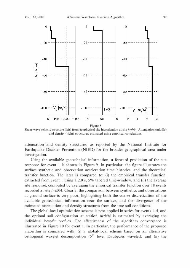
Figure 8 shows the shear-wave velocity (Vs) structure at station iwth04, based on

the geophysical site investigation, and reported at the Kik-Net Strong Motion

Network website www.kik.bosai.go.jp/kik/. Also shown, are estimates of the local

Figure 6

Selected time-window for surface to borehole empirical transfer function estimation (top), theoretical and

empirical transfer function (bottom left) and estimation residuals (bottom right) of sample time history

recorded at station IWTH04 of the Japanese Kik-Net seismic network, during the ML=4.8 aftershock (06/

10/2003 16:24) of the Miyagi earthquake.

Vol. 163, 2006 A Seismic Waveform Inversion Algorithm 97

Figure 7

Schematic representation of the proposed hybrid optimization scheme, illustrated for population j of the

genetic algorithm. The process is repeated in series for k seismograms, and the global optimum solution is

obtained by averaging k best-fit models.

98 D. Assimaki et al. Pure appl. geophys.,

attenuation and density structures, as reported by the National Institute for

Earthquake Disaster Prevention (NIED) for the broader geographical area under

investigation.

Using the available geotechnical information, a forward prediction of the site

response for event 1 is shown in Figure 9. In particular, the figure illustrates the

surface synthetic and observation acceleration time histories, and the theoretical

transfer function. The later is compared to: (i) the empirical transfer function,

extracted from event 1 using a 2.0 s, 5% tapered time-window, and (ii) the average

site response, computed by averaging the empirical transfer function over 18 events

recorded at site iwth04. Clearly, the comparison between synthetics and observations

at ground surface is very poor, highlighting both the coarse discretization of the

available geotechnical information near the surface, and the divergence of the

estimated attenuation and density structures from the true soil conditions.

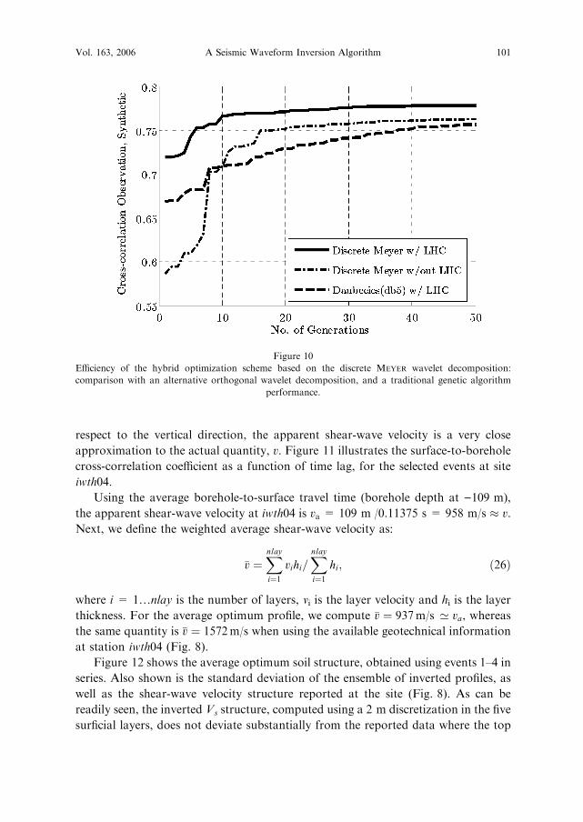
The global-local optimization scheme is next applied in series for events 1–4, and

the optimal soil configuration at station iwth04 is estimated by averaging the

individual best-fit profiles. The effectiveness of the algorithm convergence is

illustrated in Figure 10 for event 1. In particular, the performance of the proposed

algorithm is compared with: (i) a global-local scheme based on an alternative

orthogonal wavelet decomposition (5th level Daubecies wavelet), and (ii) the

Figure 8

Shear-wave velocity structure (left) from geophysical site investigation at site iwth04; Attenuation (middle)

and density (right) structures, estimated using empirical correlations.

Vol. 163, 2006 A Seismic Waveform Inversion Algorithm 99

stochastic (global) part of the algorithm, i.e., a traditional genetic algorithm. As can

be readily seen, the selected wavelet decomposition and local improvement operator

lead to faster and more effective convergence. Note also that BERSINI and RENDERS

(1994) report similar results, when comparing the hybrid optimization scheme with

traditional simulated annealing techniques.

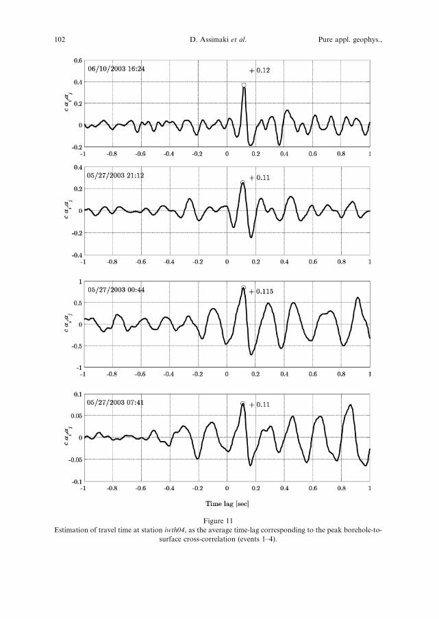
Successively, we illustrate the accuracy of the inversion in depicting the exact S-

wave arrival, by comparing the apparent velocity at station iwth04 with the weighted

average of the optimum shear-wave velocity profile. As shown in Section 2.3.2, the

apparent velocity of propagation, va, between stations i and j may be estimated from

the surface-to-borehole cross-correlation coefficient as: va = d/td, where d is the

known separation distance between stations i and j, and td is the time lag where the

cross-correlation function reaches a major peak. For small angles of incidence with

Figure 9

(a) Comparison of observation and synthetic surface response to event 1, computed using the available

local geotechnical information (Fig. 6), and (b) comparison of empirical transfer function corresponding to

event 1, theoretical (synthetic) transfer function computed using the available local geotechnical

information (Fig. 6), and average site response estimated using 28 empirical transfer functions at station

iwth04.

100 D. Assimaki et al. Pure appl. geophys.,

respect to the vertical direction, the apparent shear-wave velocity is a very close

approximation to the actual quantity, v. Figure 11 illustrates the surface-to-borehole

cross-correlation coefficient as a function of time lag, for the selected events at site

iwth04.

Using the average borehole-to-surface travel time (borehole depth at )109 m),

the apparent shear-wave velocity at iwth04 is va = 109 m /0.11375 s = 958 m/s � v.Next, we define the weighted average shear-wave velocity as:

�v ¼X

nlay

i¼1vihi=

X

nlay

i¼1hi; ð26Þ

where i = 1…nlay is the number of layers, vi is the layer velocity and hi is the layer

thickness. For the average optimum profile, we compute �v ¼ 937m/s ’ va, whereas

the same quantity is �v ¼ 1572m/s when using the available geotechnical information

at station iwth04 (Fig. 8).

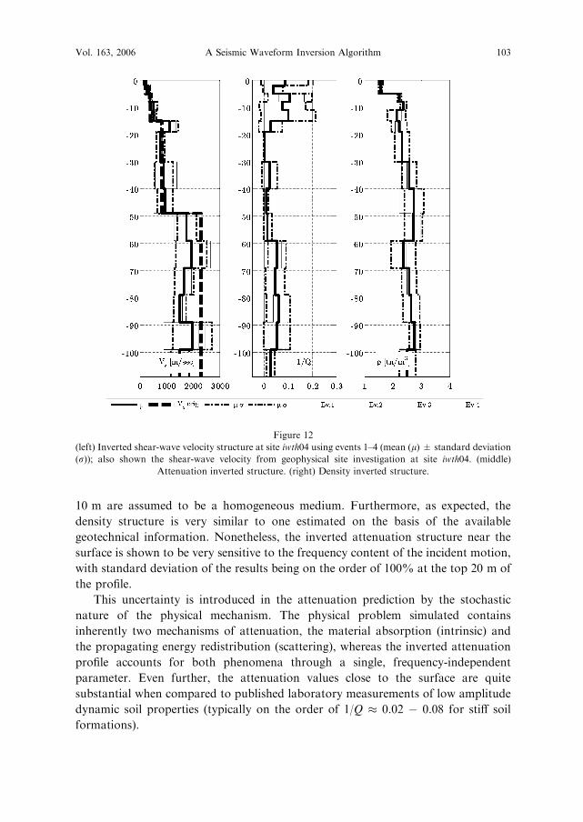
Figure 12 shows the average optimum soil structure, obtained using events 1–4 in

series. Also shown is the standard deviation of the ensemble of inverted profiles, as

well as the shear-wave velocity structure reported at the site (Fig. 8). As can be

readily seen, the inverted Vs structure, computed using a 2 m discretization in the five

surficial layers, does not deviate substantially from the reported data where the top

Figure 10

Efficiency of the hybrid optimization scheme based on the discrete MEYER wavelet decomposition:

comparison with an alternative orthogonal wavelet decomposition, and a traditional genetic algorithm

performance.

Vol. 163, 2006 A Seismic Waveform Inversion Algorithm 101

Figure 11

Estimation of travel time at station iwth04, as the average time-lag corresponding to the peak borehole-to-

surface cross-correlation (events 1–4).

102 D. Assimaki et al. Pure appl. geophys.,

10 m are assumed to be a homogeneous medium. Furthermore, as expected, the

density structure is very similar to one estimated on the basis of the available

geotechnical information. Nonetheless, the inverted attenuation structure near the

surface is shown to be very sensitive to the frequency content of the incident motion,

with standard deviation of the results being on the order of 100% at the top 20 m of

the profile.

This uncertainty is introduced in the attenuation prediction by the stochastic

nature of the physical mechanism. The physical problem simulated contains

inherently two mechanisms of attenuation, the material absorption (intrinsic) and

the propagating energy redistribution (scattering), whereas the inverted attenuation

profile accounts for both phenomena through a single, frequency-independent

parameter. Even further, the attenuation values close to the surface are quite

substantial when compared to published laboratory measurements of low amplitude

dynamic soil properties (typically on the order of 1/Q � 0.02 � 0.08 for stiff soil

formations).

Figure 12

(left) Inverted shear-wave velocity structure at site iwth04 using events 1–4 (mean (l) ± standard deviation

(r)); also shown the shear-wave velocity from geophysical site investigation at site iwth04. (middle)

Attenuation inverted structure. (right) Density inverted structure.

Vol. 163, 2006 A Seismic Waveform Inversion Algorithm 103

Note that, ideally, the best-fit average and corresponding standard deviation of

the attenuation structure should be computed on the basis of infinitely many

observations. Nonetheless, the relatively small number of events used in this case, is

based both on the target efficiency of the scheme and on the limited availability of

quality digital information, the lack of which would imply the use of a larger number

of events to achieve similar levels of confidence.

The average optimum shear-wave velocity, attenuation and density profiles

shown in Figure 12, are next subjected to the total motion recorded at the borehole

level of station iwth04 during the 4 events under investigation. Figure 13 compares

the surface measured and synthetic ground motions both in the time and frequency

domain, for the 2 sec time-window used in the optimization process.

As can be readily seen, the proposed scheme can accurately depict both the

frequency content and amplitude of the recorded surface ground motion. It should

be noted, however, that the complexity of the measured process, clearly manifesting

in the frequency response of the system, highlights further the stochastic nature of the

physical problem, which is not captured by simplified mathematical models.

The limitations of our forward numerical simulation, which attempts to

approximate 3D strongly heterogeneous systems by means of 1D horizontally

stratified homogeneous configurations, can be also illustrated by comparing the

synthetic and measured rate of incident seismic energy at ground surface.

In the time domain, the energy of the direct wave can be expressed as the

summation of the squared amplitudes in the window containing the direct arrival

(FRANKEL and WENNERBERG, 1987; KORN, 1997). To estimate the normalized seismic

energy, we first compute the wave energy in an appropriate time-window as follows:

EiðtmÞ ¼Z

t2

t1

A2i ðtÞ dt; ð27Þ

where A2i ðtÞ is the square-wave amplitude at the ith station at time t, and tm is the

central time (mid-point) of the window between t1 and t2. Successively, the energy

estimated in each window is normalized by the total energy of the waveform, starting

from the S-wave arrival to the end (90% of the total incident energy) of the waveform

under consideration. Therefore, the normalized energy arriving at station i at time tmis defined as:

�EiðtmÞ ¼

R

t2

t1

A2i ðtÞ dt

R

T90

tS

A2i ðtÞ dt

; ð28Þ

where tS is the S-wave arrival time, and T90 is the lapse time that corresponds to 90%

of the total incident wave energy. The normalized energy time history, computed by

104 D. Assimaki et al. Pure appl. geophys.,

Figure 13

(a) Comparison of surface observations and global optimum synthetics at station iwth04, for events 1–4,

and (b) comparison of empirical transfer function corresponding to the individual events (light continuous

line), theoretical transfer function computed for the individual best-fit models (dark dashed line), and

theoretical transfer function computed for the global optimum model (dark continuous line).

Vol. 163, 2006 A Seismic Waveform Inversion Algorithm 105

sliding the window [t1, t2] across the waveform, is referred to as the energy partition

pattern (SIVAJI et al., 2002).

Figure 14 plots the energy partition pattern for events 1–4 at station iwth04.

Comparison of the measured and optimal synthetic surface motions shows good

agreement both of the incident energy rate and the maximum energy level at ground

surface. Nonetheless, the synthetic energy partition has larger gradient at early times,

indicative of the coherent energy incidence for the horizontally stratified homoge-

neous medium, as opposed to the heterogeneous real configuration. Even assuming

vertical incidence at the borehole level for the later: (i) the first arrival of seismic

energy would be still delayed due to multiple scattering, and (ii) this phenomeno-

logical energy attenuation would be successively counteracted by non-vertically

propagating waves, scattered from adjacent locations within the same profile.

4. Sensitivity Analysis on the Inverted Attenuation Structure

As illustrated above, the best-fit attenuation structure is strongly dependent on

the frequency content of the seismogram used in the inversion scheme, stemming

from the stochastic nature of the physical process. In particular, uncertainties

introduced in the measured process by means of material heterogeneities and incident

Figure 14

Energy partition pattern at ground surface, computed for events 1–4 at station iwth04: Comparison

between observations and synthetics, computed using the global optimum solution.

106 D. Assimaki et al. Pure appl. geophys.,

motion variability, result to observations where the elastic site response is time- and

frequency-content dependent. Based on results illustrated in Section 3, such

limitations of the mathematical model are strongly reflected on the inverted

attenuation profile, unlike the estimated impedance structure.

To illustrate this concept, Figure 15 depicts the temporal variability of the

empirical transfer function recorded at station iwth04, during the ML=4.8

aftershock (06/10/2003 16:24) of the Miyagi earthquake. For this purpose, we apply

a 2.2 s, 5% tapered sliding window, and compute the surface and borehole frequency

spectra and the corresponding empirical transfer functions. The latter is estimated as

the amplitude of the complex Fourier spectral ratio of the surface to borehole

motion. As can be readily seen, the relatively uniform site response, which

corresponds to the first S-wave arrival (t = 22.80 s), is followed by a highly erratic

region. Unlike the former, the response is here governed by late arrivals of scattered

energy interacting with waves trapped within the strongly heterogeneous, near

surficial layers.

To identify the time window for which the shifted borehole and surface motion

show maximum coherency, we compute the cross-correlation coefficient at zero time

Figure 15

(a) Borehole and (b) surface acceleration spectrograms of event 1, recorded at station iwth04; (c) transfer

function amplitude spectrogramat the same location.Note that the S-wave arrival is estimated at t=22.80 s,

corresponding to the end of the coherent site response region of the spectrogram.

Vol. 163, 2006 A Seismic Waveform Inversion Algorithm 107

lag (cai; ajð0Þ in eq. (25)) using a 2.0 s sliding time-window, and plot its temporal

variation in Figure 16. The local maximum of the coherence function in the region of

the S arrival, corresponds to the time-window that starts exactly at the S-wave

arrival, and from this point on, the cross-correlation degrades due to scattering

phenomena that contaminate the uniform response.

Successively, we investigate the effects of the time-window duration, namely the

trade-off between the available information on the process to be simulated, and the

uncertainty introduced by non-simulated phenomena. As shown above, we overcome

this uncertainty that manifests in the inverted attenuation structure, by averaging

multiple best-fit models at the same station, thus obtaining a robust global optimum

solution. In the ensuing, we attempt to achieve a more stable local average site

response by computing the inverted soil structure at station iwth04 using a 10 s time-

window initiating at the S-wave arrival.

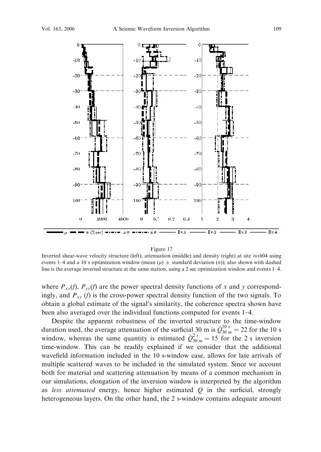
Figure 17 shows the average optimum soil structure, obtained using the 10 s time-

window and events 1–4 in series. Also shown is the standard deviation of the ensemble

of inverted profiles, as well as the shear-wave velocity structure reported at the site

(Fig. 8) and the optimum structure computed using a 2 s time-window (Fig. 12).

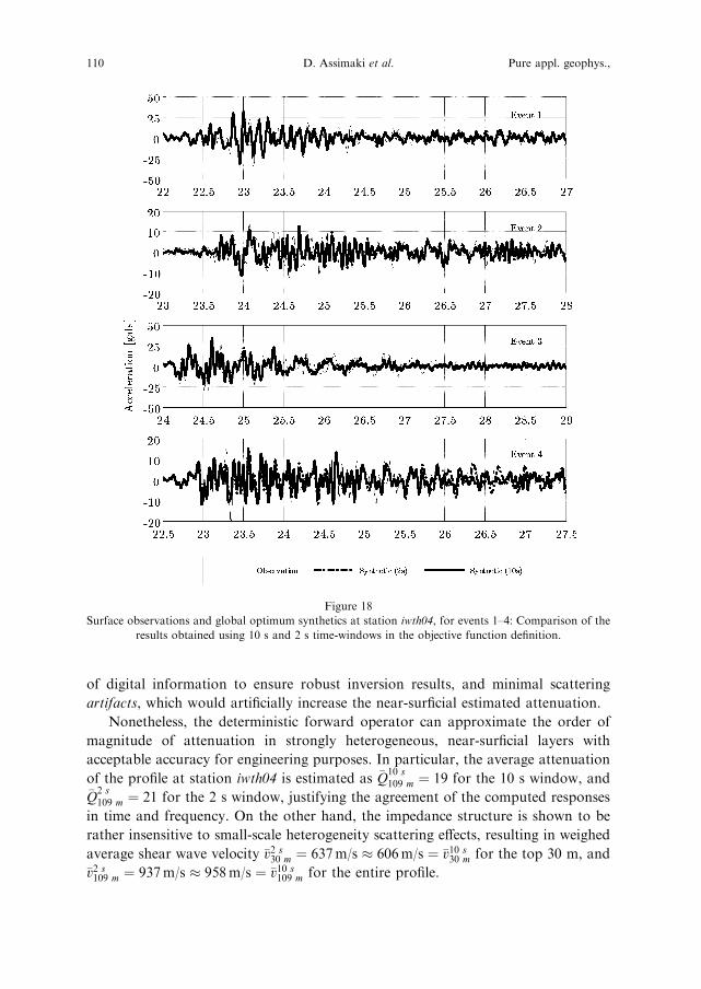
Successively, Figure 18 compares the surface recorded and synthetic time-histories,

for the 10 s and 2 s inversion time-windows. As can be readily seen, results obtained

by means of the two inversions are in very good agreement, supported also by the

optimum synthetic-observation cross-correlation computed for events 1–4 (Table 1).

Finally, Figure 19 illustrates the consistency of the two approaches in the

frequency domain, by comparing the optimum synthetic-to-observation coherence

spectra computed using sliding 5% tapered time-windows with 25% overlap, and

durations 2 s and 10 s, correspondingly. In particular, we plot the magnitude-

squared coherence estimate Cxy of the observation, x, and synthetic, y, signals using

Welch’s averaged, modified periodogram method, as follows:

cxy ¼jPxyðf Þj2

Pxxð f Þ � Pyyð f Þ; ð29Þ

Figure 16

Surface to borehole cross-correlation coefficient for the event described above. The coefficient

corresponding to the S-arrival window used in the inversion scheme is also indicated.

108 D. Assimaki et al. Pure appl. geophys.,

where Pxx(f), Pyy(f) are the power spectral density functions of x and y correspond-

ingly, and Pxy (f) is the cross-power spectral density function of the two signals. To

obtain a global estimate of the signal’s similarity, the coherence spectra shown have

been also averaged over the individual functions computed for events 1–4.

Despite the apparent robustness of the inverted structure to the time-window

duration used, the average attenuation of the surficial 30 m is �Q10 s30 m ¼ 22 for the 10 s

window, whereas the same quantity is estimated �Q2 s30 m ¼ 15 for the 2 s inversion

time-window. This can be readily explained if we consider that the additional

wavefield information included in the 10 s-window case, allows for late arrivals of

multiple scattered waves to be included in the simulated system. Since we account

both for material and scattering attenuation by means of a common mechanism in

our simulations, elongation of the inversion window is interpreted by the algorithm

as less attenuated energy, hence higher estimated Q in the surficial, strongly

heterogeneous layers. On the other hand, the 2 s-window contains adequate amount

Figure 17

Inverted shear-wave velocity structure (left), attenuation (middle) and density (right) at site iwth04 using

events 1–4 and a 10 s optimization window (mean (l) ± standard deviation (r)); also shown with dashed

line is the average inverted structure at the same station, using a 2 sec optimization window and events 1–4.

Vol. 163, 2006 A Seismic Waveform Inversion Algorithm 109

of digital information to ensure robust inversion results, and minimal scattering

artifacts, which would artificially increase the near-surficial estimated attenuation.

Nonetheless, the deterministic forward operator can approximate the order of

magnitude of attenuation in strongly heterogeneous, near-surficial layers with

acceptable accuracy for engineering purposes. In particular, the average attenuation

of the profile at station iwth04 is estimated as �Q10 s109 m ¼ 19 for the 10 s window, and

�Q2 s109 m ¼ 21 for the 2 s window, justifying the agreement of the computed responses

in time and frequency. On the other hand, the impedance structure is shown to be

rather insensitive to small-scale heterogeneity scattering effects, resulting in weighed

average shear wave velocity �v2 s30 m ¼ 637m/s � 606m/s ¼ �v10 s

30 m for the top 30 m, and

�v2 s109 m ¼ 937m/s � 958m/s ¼ �v10 s

109 m for the entire profile.

Figure 18

Surface observations and global optimum synthetics at station iwth04, for events 1–4: Comparison of the

results obtained using 10 s and 2 s time-windows in the objective function definition.

110 D. Assimaki et al. Pure appl. geophys.,

To complete the parametric investigation on the attenuation structure sensitivity

to the inversion objective function, we compute the optimum profile at station iwth04

using: (i) the average elastic site response in the frequency domain (estimated using

10 s time-windows for the ensemble of 28 low-amplitude seismograms recorded at

the station) as objective function of the genetic algorithm, and (ii) only the average

borehole-to-surface travel time as objective function of the local hill-climbing

operator. Based on the stability of the estimated travel time illustrated for four events

in Figure 11, and the erratic behavior of the empirical transfer functions in the high-

frequency region, we thus attempt to further minimize the effects of the stochastic

nature of the physical process.

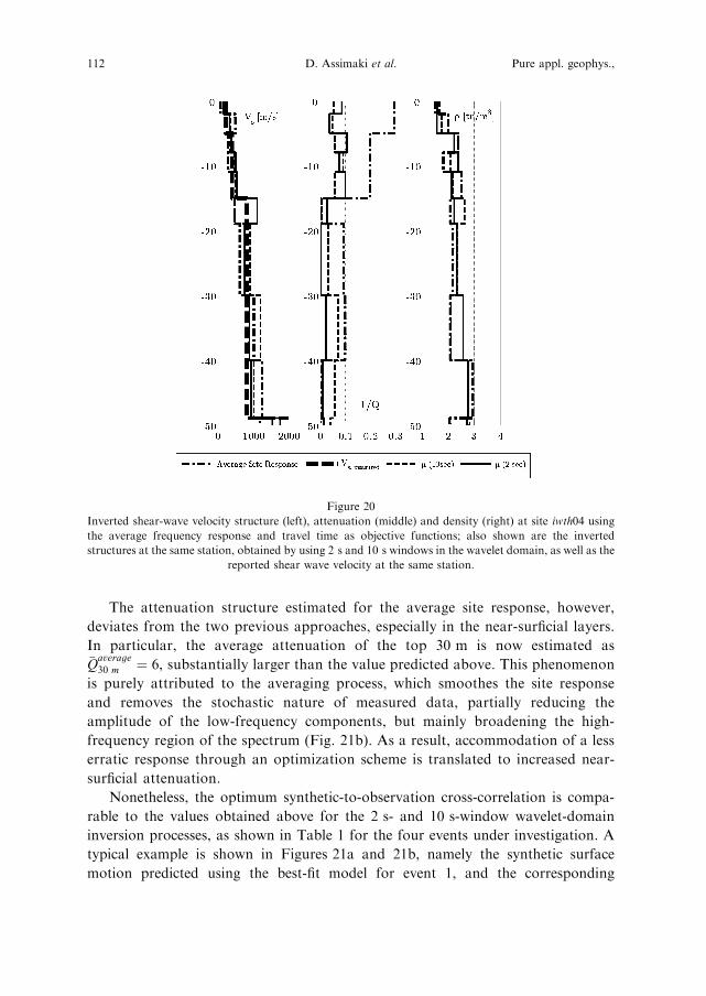
Figure 20 shows the global optimum soil structure obtained, compared to the

average inverted structure of the original (2 s window) and alternative (10 s window)

hybrid optimization schemes. As can be readily seen, the inverted velocity and

density structures are in good agreement, illustrating the effectiveness of the

algorithm to capture the upgoing and downgoing reflections and refractions of the

seismic energy within the multiple horizontally stratified soil layers.

Figure 19

Coherence function spectra of surface observations and global optimum synthetics at station iwth04,

averaged over events 1–4: Comparison of the results obtained using 10 s and 2 s time-windows in the

objective function definition.

Table 1

Optimum synthetic-to-observation normalized cross-correlation at site iwth04 for events 1–4: Comparison of

the wavelet domain optimization scheme with 2 s and 10 s time-windows, and the borehole-to-surface average

travel time and frequency site response as objective functions

Event 1 Event 2 Event 3 Event 4

2 s window 0.79516 0.6144 0.78051 0.48173

10 s window 0.70232 0.56498 0.69949 0.60906

Average TF 0.75992 0.55174 0.68579 0.51451

Vol. 163, 2006 A Seismic Waveform Inversion Algorithm 111

The attenuation structure estimated for the average site response, however,

deviates from the two previous approaches, especially in the near-surficial layers.

In particular, the average attenuation of the top 30 m is now estimated as�Qaverage30 m ¼ 6, substantially larger than the value predicted above. This phenomenon

is purely attributed to the averaging process, which smoothes the site response

and removes the stochastic nature of measured data, partially reducing the

amplitude of the low-frequency components, but mainly broadening the high-

frequency region of the spectrum (Fig. 21b). As a result, accommodation of a less

erratic response through an optimization scheme is translated to increased near-

surficial attenuation.

Nonetheless, the optimum synthetic-to-observation cross-correlation is compa-

rable to the values obtained above for the 2 s- and 10 s-window wavelet-domain

inversion processes, as shown in Table 1 for the four events under investigation. A

typical example is shown in Figures 21a and 21b, namely the synthetic surface

motion predicted using the best-fit model for event 1, and the corresponding

Figure 20

Inverted shear-wave velocity structure (left), attenuation (middle) and density (right) at site iwth04 using

the average frequency response and travel time as objective functions; also shown are the inverted

structures at the same station, obtained by using 2 s and 10 s windows in the wavelet domain, as well as the

reported shear wave velocity at the same station.

112 D. Assimaki et al. Pure appl. geophys.,

theoretical transfer function, compared to the one obtained for the global optimal

model of the original hybrid optimization scheme (2 s window).

5. Conclusions

We have presented an efficient hybrid optimization scheme for downhole array

seismogram inversion, which combines a traditional genetic algorithm defined in the

wavelet domain, with a local hill-climbing operator, namely a nonlinear least-squares

optimization, in the frequency domain. The proposed algorithm has the following

advantages: (i) using normalized wavelet decomposition of the ground surface

seismograms, we assign equal weight across all frequency bands of interest and

achieve high observation-synthetic cross-correlation throughout the 1–15 Hz fre-

quency range, and (ii) while locally improving the parental population of each

generation in the genetic algorithm, we considerably accelerate the convergence rate

of the inversion scheme, compared to traditional genetic algorithms.

To eliminate the observation error propagation and the limitations of our

forward numerical model, which does not account for small-scale material

heterogeneities, we repeat the inversion process in series for multiple recordings

selected on the basis of their signal quality, and define the global optimum solution as

the average structure of the individual best-fit models. Our results of the optimum

structure response to the borehole recorded seismic motions, show very good

agreement with the corresponding ground surface observations. While a single

station is used in this paper to illustrate the application of the proposed

methodology, results from weak and strong motion events recorded at multiple

Kik-Net stations will be presented in a forthcoming paper by the authors.

Performing sensitivity analysis on the inverted attenuation structure, we observed

high dependence of the best-fit solution both on the frequency content of the

recorded ground motion and on the time-window used in the definition of the

optimization objective function. This is attributed to the simplifications of our

mathematical model, which cannot simulate the physical process by representing

material and scattering attenuation simultaneously by means of the single frequency-

independent parameter Q. It should be noted that the alternative of frequency-

dependent attenuation, expressed as Q = a f b, where f is the frequency and a, b are

the optimization parameters, was also considered in our preliminary simulations and

yielded similar fluctuations in the inverted structure, primarily due to instabilities of

the estimated exponent b.

Our conclusions suggest that the criteria for successful ground motion

predictions should extend to include simulated systems, which are in good

agreement with the observations but also approximate well the physical process.

In particular for the qualitative estimation of site response in engineering

applications, simultaneous modeling of material absorption and scattering atten-

Vol. 163, 2006 A Seismic Waveform Inversion Algorithm 113

uation in the form of viscous damping might lead to underestimation of the surface

ground motion.

Since scattering attenuation is the mathematical expression of energy redistribu-

tion, geoprocesses shown to be significantly affected by micro-scale heterogeneities,

cannot be accurately simulated based on the assumption of scattering energy loss.

Examples include the soil response during liquefaction (POPESCU and PREVOST, 1996;

POPESCU et al., 1997; KOKUSHO, 1999); the spatial variability of surface ground

motion (ASSIMAKI et al., 2003; NOUR et al., 2003); slope instability (YONG et al.,

1977; TONON et al., 2000), settlement (PAICE et al., 1996) and seepage (GRIFFITHS

and FENTON, 1993; FENTON and GRIFFITHS, 1996) in porous media; and soil-

structure interaction (ZERVA, 1991). In particular for high-frequency components

of seismic waves propagating through the near-surficial, highly heterogeneous

formations, deviation of our predictions from the physical process might be quite

Figure 21

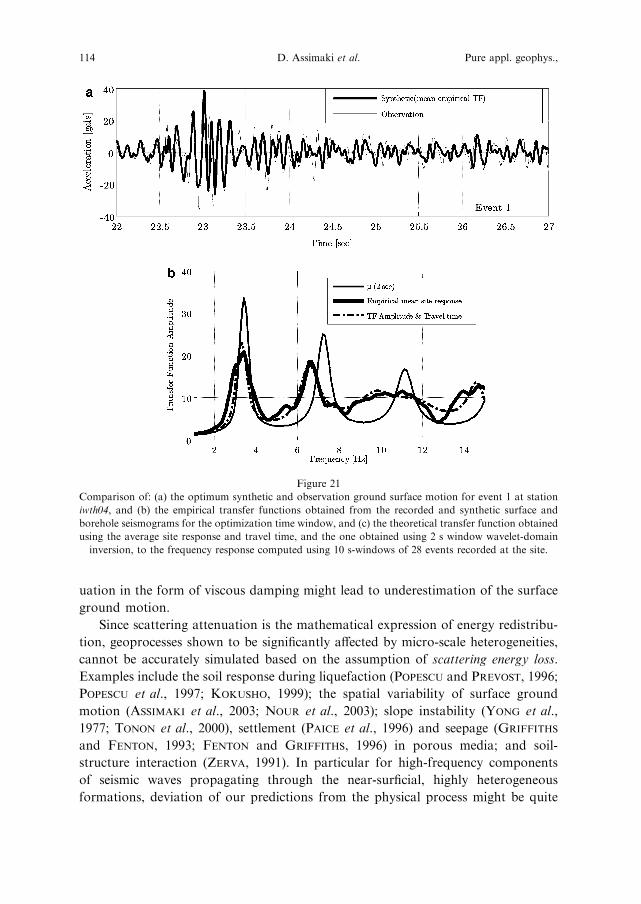
Comparison of: (a) the optimum synthetic and observation ground surface motion for event 1 at station

iwth04, and (b) the empirical transfer functions obtained from the recorded and synthetic surface and

borehole seismograms for the optimization time window, and (c) the theoretical transfer function obtained

using the average site response and travel time, and the one obtained using 2 s window wavelet-domain

inversion, to the frequency response computed using 10 s-windows of 28 events recorded at the site.

114 D. Assimaki et al. Pure appl. geophys.,

substantial, due to the length-scale similarity of soil layering, heterogeneity

correlation distances, wavelengths of the propagating energy, and the inability to

specify the model structure at this scale.

Downhole array recordings therefore, are ideal for studies on the effectiveness of

existing inversion schemes, and also for the development of future algorithms, aiming

both to simulate the process and capture the mechanisms by which the physical

system causes the two distinct forms of attenuation.

Acknowledgments

This research was partially supported by the Southern California Earthquake

Center No. 0878; SCEC is funded by NSF Cooperative Agreement EAR-0106924

and USGS Cooperative Agreement 02HQAG0008. Additional support was provided

by the Institute for Crustal Studies No. 0691, at the University of California, Santa

Barbara, CA 93105.

REFERENCES

ABERCROMBIE, R.E. (1995), Earthquake source scaling relationships from )1 to 5 ML using seismograms

recorded at 2.5 km depth, J. Geophys. Res. 100, 24,015–024,036.

ABERCROMBIE, R. E. (1997), Near-surface attenuation and site effects from comparison of surface and deep

borehole recording, Bull. Seism. Soc. Am. 87, 731–744.

AGUIRRE, J. and IRIKURA, K. (1997), Nonlinearity, liquefaction, and velocity variation of soft soil layers in

Port Island, Kobe, during the Hyogoken Nanbu Earthquake, Bull. Seismol. Soc. Am. 87, 1244–1258.

ASSIMAKI, D., PECKER, A., POPESCU, R., and PREVOST, J.H. (2003), Effects of spatial variability of soil

properties on surface ground motion, J. Earthq. Engin. 7(1), 1–44.

BENDAT, J.S. and PIERSOL, A.G. (1996), Engineering Applications of Correlation and Spectral Analysis, 2nd

ed., 458 pp. (John Wiley and Sons, Inc).

BERSINI, H. and RENDERS, B. (1994), Hybridizing genetic algorithms with hill-climbing methods for global

optimization: Two possible ways, Paper presented at IEEE Internat. Symp. Evol. Comput., Orlando, FL.

BOORE, D.M. and JOYNER, W.B. (1997), Site amplification for generic rock sites, Bull. Seismol. Soc. Am. 87,

327–341.

BRUNE, J.N. (1970), Tectonic stress and the spectra of seismic shear waves from earthquakes, J. Geophys.

Res. 75, 4,997–5,009.

BRUNE, J.N. (1971), Correction, J. Geophys. Res. 76, 5,002.

CHUI, C.K. (1992),Wavelets - A Tutorial in Theory and Applications (Wavelet Analysis and its Applications,

vol. 2) (Academic, San Diego, CA).

CORANA, A. et al. (1987), Minimizing multimodal functions of continuous variables with the ‘‘simulated

annealing’’ algorithm, ACM Transac. Math. Software 13, 262–280.

DAUBECHIES, I. (1988), Orthonormal basis of compactly supported wavelets, Com. Pure Appl. Math. XLI,901–996.

DAUBECHIES, I. (1992), Ten Lectures on Wavelets, 357 pp., Society for Ind. and Appl. Math. Philadelphia,

PA.

DAVIS, L. (1991), The Handbook of Genetic Algorithms (Van Nostrand Reingold, New York).

EARTHQUAKE SPECTRA (2000), 1999 Kocaeli, Turkey, Earthquake Reconnaissance Report, Supplement A to

volume 16, December.

Vol. 163, 2006 A Seismic Waveform Inversion Algorithm 115

FENTON, G.A. and GRIFFITHS, D.V. (1996), Statistics of free surface flow through stochastic earth dam,

J. Geotech. Engin. 122(6), 427–436.

FOUFOULA-GEORGIOU, E. and KUMAR, P. (1994), Wavelets in Geophysics, 384 pp. (Academic, San Diego,

CA).

FRANKEL, A. and WENNERBERG, L. (1987), Energy-flux model of seismic coda: Separation of scattering and

instrinsic attenuation, Bull. Seismol. Soc. Am. 77, 1223–1251.

GOLDBERG, D. (1989), Genetic Algorithms in Search, Optimization, and Machine Learning (AddisonWes-

ley).

GOUPILLAUD, P.A. et al. (1984), Cycle-octaves and related transforms in seismic signal analysis,

Geoexploration 23, 85–102.

GRIFFITHS, D.V. and FENTON, G.A. (1993), Seepage beneath water retaining structures founded on spatially

random soil, Geotechnique 43(4), 577–587.

GROSSMANN, A. and MORLET, J. (1984), Decomposition of handy functions into square integrable wavelets of

constant shape, SIAM J. Math. Analysis 15, 723–736.

GUSTAFSSON, F. (1996), Determining the initial states in forward-backward filtering, IEEE Transact. Signal

Processing 44, 988–993.

HARTZELL, S.H. et al. (1996), The 1994 Northridge, California, earthquake: Investigation of rupture velocity,

rise time and high-frequency radiation, J. Geophys. Res. 101, 20,091–020,108.

HARTZELL, S.H., LEEDS, A., FRANKEL, A., and MICHAEL, J. (1996), Site response for urban Los Angeles

using aftershocks of the Northridge Earthquake, Bull. Seismol. Soc. Am. 86, 5168–5192.

HOLLAND, J. (1975), Adaptation in Natural and Artificial Systems (The University of Michigan Press, Ann

Arbor).

HOLSCHNEIDER, M. (1995), Wavelets: An analysis Tool, 423 pp. (Oxford University Press, New

York).

HOUCK, C.R. et al. (1996), Comparison of genetic algorithms, random restart and two-opt switching for

solving large location-allocation problems, Computers and Operations Res. 23, 587–596.

HOUSNER, G.W. (1990), Competing against time, Report to Governor George Deukmejian from the

Governor’s Board of Inquiry on the 1989 Loma Prieta Earthquake.

IAI, S., MORITA, T., KAMEOKA, T., MATSUNAGA, Y., and ABIKO, K. (1995), Response of a dense sand

deposit during 1993 Kushiro-Oki Earthquake, Soils and Foundations 35, 115–131.

JI, C., WALD, D., and HELMBERGER, D. (2002), Source description of the 1999 Hector Mine, California,

Earthquake, Part I: Wavelet domain inversion theory and resolution analysis, Bull. Seismol. Soc. Am. 92,

1192–1207.

JOINES, J. and HOUCK, C. (1994), On the use of non-stationary penalty functions to solve constrained

optimization problems with genetic algorithms, Paper presented at IEEE Internat. Symp. Evolut. Comput.

Orlando, FL.

KINOSHITA, S. (1992), Local Characteristic of the fmax of bedrock motion in the Tokyo metropolitan area,

Japan, J. Phys. Earth 40, 487–515.

KOKUSHO, T. (1999), Water film in liquefied sand and its effect on lateral spread, J. Geotech. Geoenviron.

Eng. 125(10), 817–826.

KORN, M. (1997), Modelling of teleseismic P coda envelope: Depth-dependent scattering and deterministic

structure, Phys. Earth Planet. Inter. 104, 23–36.

MADARIAGA, R. (1976), Dynamics of an expanding circular fault, Bull. Seismol. Soc. Am. 66, 639–667.

MALLAT, S. (1989a), A theory for multiresolution signal decomposition: The wavelet representation, IEEE

Transact. Pattern Analysis and Machine Intelligence 11, 674–693.

MALLAT, S. (1989b), Multifrequency channel decomposition of images and wavelet models, IEEE Transact.

Acoustic Speech and Signal Analysis 37, 2091–2110.

MATHWORKS (1993), MATLAB: Signal Processing Toolbox, User’s Guide.

MEYER, Y. (1992), Wavelets and Operators (Cambridge University Press, New York).

MICHALEWICZ, Z. (1994), Genetic Algorithms + Data Structures = Evolution Programs (Springer-Verlag,

New York).

MORLET, J. et al. (1982a), Wave propagation and sampling theory: I. Complex signal and scattering in

multilayered media, Geophys. 47, 203–221.

116 D. Assimaki et al. Pure appl. geophys.,

MORLET, J. et al. (1982b), Wave propagation and sampling theory: II. Sampling theory and complex waves,

Geophys. 47, 222–236.

NOUR, A., SLIMANI, A., LAOUAMI, N., and AFRA, H. (2003), Finite element model for the probabilistic

seismic response of heterogeneous soil profile, Soil Dyn. Earthq. Engin. 23, 331–348.

OHSAKI, Y. (1969), The effects of local soil conditions upon earthquake damage, Proc. Specialty Session on

Soil Dynamics, 7th ICSMFE.

PAICE, G.M., GRIFFITHS, D.V., and FENTON, G.A. (1996), Finite element modeling of settlements on

spatially random soil, J. Geotech. Engin. 122(9), 777–779.

POPESCU, R. and PREVOST, J.H. (1996), Influence of spatial variability of soil properties on seismically

induced soil liquefaction, Geotech. Special Pub. 58, 1098–1112.

POPESCU, R., PREVOST, J.H., and DEODATIS, G. (1997), Effects of spatial variability on soil liquefaction:

Some design recommendations, Geotechnique 47(5), 1019–1036.

ROSENBLUETH, E. (1960), Earthquake of 28 July 1957 in Mexico City, Proc. 2nd WCEE, 1, pp. 359–

379.

SATO, K., KOKUSHO, T., MATSUMOTO, M., and YAMADA, E. (1996), Nonlinear seismic response and soil

property during strong motion, in Special Issue of Soils and Foundations in Geotechnical Aspects of the

January 17, 1995, Hyogoken-Nambu Earthquakes, pp. 41–52.

SATOH, T., FUSHIMI, M., and TATSUMI, Y. (2001), Inversion of strain-dependent nonlinear characteristics of

soils using weak and strong motions observed by boreholes sites in Japan, Bull. Seismol. Soc. Am. 91, 365–

380.

SATOH, T., KAWASE, H., and SATO, T. (1995), Evaluation of local site effects and their removal from borehole

records observed in the Sendai region, Japan, Bull. Seismol. Soc. Am. 85, 1770–1789.

SEED, H.B. and ROMO, M.P. (1987), Relationships between soil conditions and earthquake ground motions in

Mexico City in the earthquake of September 19, 1985, Report No. EERC-87–15, University of

California, Berkeley.

SEED, H.B., WHITMAN, R.V., DEZFULIAN, H., DOBRY, R., and IDRISS, I.M. (1972), Soil conditions and

damage in the 1967 Caracas Earthquake, J. Soil Mech. Foundations, ASCE 98, 787–806.

SEED, H.B. and IDRISS, I.M. (1970), Analyses of ground motions at Union Bay, Seattle during earthquakes

and distant nuclear blasts, Bull. Seismol. Soc. Am. 60, 125–136.

SIVAJI, C. et al. (2002), A physical-model study of the statistics of seismic waveform fluctuations in random

heterogeneous media, Geophys. J. Internat. 148, 575–595.

SNIEDER, R. and TRAMPERT, J. (1999), Inverse problems in Geophysics, in Wavefield Inversion (ed. A.

Wirgin) (Springer Verlag, New York), pp. 119–190.

SOIL, and FOUNDATIONS (1996), Special issue on Geotechnical Aspects of the January 17, 1995 Hyogoken-

Nambu Earthquake, January.

STEIDL, J.H., TUMARKIN, A.G., and ARCHULETA, R.J. (1996), What is a reference site? Bull. Seismol. Soc.

Am. 86, 1733–1748.

STOFFA, P.L. and SEN, M.K. (1991), Nonlinear multiparameter inversion using genetic algorithms: Inversion

of plane-wave seismograms, Geophysics 56, 1794–1810.

TEZCAN, S.S., YERLICI, V., and DURGUNOGLOU, H.T. (1979), A reconnaissance report for the Romanian

earthquake of 4 March 1977, Engin. Struct. Dyn. 6, 397–421.

TONON, F., BERNARDINI, A., and Mammino, A. (2000), Reliability analysis of rock mass response by means

of random set theory, Reliability Engin. Systems Safety 70(3), 263–282.

TRAMPERT, J. (1998), Global seismic tomography: the inverse problem and beyond, Inverse Problems 14,

371–385.

WEN, K., BERESNEV, I., and YEH, Y.T. (1994), Nonlinear soil amplification inferred from downhole strong

seismic motion data, Geophys. Res. Lett. 21, 2625–2628.

WORNELL, G.W. (1995), Signal Processing with Fractals: A Wavelet-based Approach (Prentice-Hall,

Englewood Cliffs, N.J).

YONG, R.N., ALONSO, E., and TABBA, M.M. (1977), Application of risk analysis to the prediction of slope

stability, Canadian Geotech. J. 14(4), 540–553.

ZEGHAL, M. and ELGAMAL, A.W. (1994), Analysis of site liquefaction using earthquake records, J. Geotech.

Engin. 120(6), 996–1017.

Vol. 163, 2006 A Seismic Waveform Inversion Algorithm 117

ZERVA, A. (1991), Effect of spatial variability and propagation of seismic ground motions on the response of

multiply supported structures, Prob. Engin. Mech. 6, 212–221.

(Received March 9, 2005; accepted July 19, 2005)

To access this journal online:

http://www.birkhauser.ch

118 D. Assimaki et al. Pure appl. geophys.,