Australian groundwater modelling guidelines - National Centre for

NATIONAL WATER COMMISSION WATERLINES i

Australian groundwater modelling guidelines

Sinclair Knight Merz and National Centre for Groundwater Research

and Training

Waterlines Report Series No 82 June 2012

mdash

Waterlines

This paper is part of a series of works commissioned by the National Water Commission on

key water issues This work has been undertaken by Sinclair Knight Merz and the National

Centre for Groundwater Research and Training on behalf of the National Water Commission

copy Commonwealth of Australia 2012

This work is copyright

Apart from any use as permitted under the Copyright Act 1968 no part may be reproduced by any process without prior written permission

Requests and enquiries concerning reproduction and rights should be addressed to the Communications Director National Water Commission 95 Northbourne Avenue Canberra ACT 2600 or email bookshopnwcgovau

Onlineprint ISBN 978-1-921853-91-3

Australian groundwater modelling guidelines June 2012 Authors Barnett B Townley LR Post V Evans RE Hunt RJ Peeters L Richardson S Werner AD Knapton A and Boronkay A

Published by the National Water Commission 95 Northbourne Avenue Canberra ACT 2600 Tel 02 6102 6000 Email enquiriesnwcgovau

Date of publication June 2012

Cover design by Angelink Front cover image courtesy of Sinclair Knight Merz Pty Ltd

An appropriate citation for this report is Barnett et al 2012 Australian groundwater modelling guidelines Waterlines report National Water Commission Canberra

Disclaimer

This paper is presented by the National Water Commission for the purpose of informing

discussion and does not necessarily reflect the views or opinions of the Commission In

addition see separate disclaimer for Chapter 7 on the acknowledgements page

Contents Acknowledgements ix Executive summary x 1 Introduction1

11 Overview 1 12 Structure of the guidelines 2 13 Need for and use of the guidelines 3 14 What are groundwater models4 15 Fundamentals of groundwater and modelling5 16 The modelling process11

2 Planning14 21 Introduction 14 22 Intended use of the model 15 23 Defining modelling objectives 16 24 Initial consideration of investigation scale16 25 Model confidence level classification17 26 Defining exclusions 22 27 Review and update 23 28 Model ownership23

3 Conceptualisation 24 31 Introduction 24 32 The principle of simplicity25 33 Conceptualisation of current and future states 26 34 Alternative conceptual models 26 35 Data collection analysis and data checking 27 36 Developing the conceptual model28 37 Checking the conceptual model32 38 3D visualisation33 39 Conceptualisation as an ongoing process 34 310 Reporting and review 35

4 Design and construction36 41 Introduction 36 42 Numerical method37 43 Software 39 44 Model domain 47 45 Boundary conditions 53 46 Initial conditions 54 47 Model construction55

5 Calibration and sensitivity analysis57 51 Introduction 58 52 Fundamental concepts58 53 Calibration methodologies 65 54 Challenges and solutions69 55 Sensitivity analysis77 56 Verification 78

6 Prediction79 61 Introduction 79 62 Predictive model time domain81 63 Modelling extraction from wells82 64 Climate stresses in predictions 85 65 Particle tracking 86 66 Predicting pore pressures 87 67 Predicting groundwater responses to underground construction 87 68 Annual aquifer accounting models90 69 Checking model results90

7 Uncertainty 92 71 Introduction 92

NATIONAL WATER COMMISSION mdash WATERLINES iv

72 The concept of uncertainty93 73 Sources of model uncertainty 95 74 Relation of model calibration to model uncertainty98 75 Common approaches for estimating uncertainty 99 76 Communicating model uncertainty to decision makers 103

8 Reporting 106 81 Introduction 106 82 Staged reporting 106 83 Target audience 107 84 Structure107 85 Visualisation109 86 Archiving 116

9 Reviews 117 91 Introduction 117 92 Review process117 93 Review checklists119

10 Focus topic Solute transport125 101 Introduction 126 102 When to use a solute transport model 126 103 Fundamental concepts128 104 Conceptualisation 132 105 Design and construction 143 106 Calibration and sensitivity analysis 150 107 Prediction and uncertainty 151 108 Reporting153

11 Focus topic Surface waterndashgroundwater interaction 154 111 Introduction 155 112 Fundamental concepts156 113 Conceptualisation 162 114 Design and construction 167 115 Calibration and sensitivity analysis 177 116 Prediction and uncertainty 178 117 Reporting179

References 180 Appendix AmdashSummary of existing groundwater flow modelling texts standards and guidelines187

Tables

Table 2-1 Model confidence level classificationmdashcharacteristics and indicators 20 Table 4-1 Modelling software commonly used in Australia 42 Table 4-2 Issues to consider when selecting a model code and GUI 45 Table 4-3 Recommended model codes for non-conventional groundwater

settings 47 Table 4-4 Examples of different model dimensions 48 Table 5-1 Performance measures and targets 74 Table 8-1 Example final model report structure (modified after MDBC 2001) 109 Table 9-1 Compliance checklist119 Table 9-2 Review checklist 120 Table 10-1 Total porosity values for varying lithological units 141 Table 11-1 Differences between surface water and groundwater161 Table 11-2 MODFLOW packages relevant to surface waterndashgroundwater

interaction 174 Table 11-3 Examples of different levels of detail176

NATIONAL WATER COMMISSION mdash WATERLINES v

Figures

Figure 1-1 A schematic cross-section showing a groundwater system with unconfined and confined aquifers and connectivity between a surface water body (a lake) and the shallow groundwater 7

Figure 1-2 Groundwater modelling process (modified after MDBC 2001 and Yan et al 2010)13

Figure 2-1 The planning process15 Figure 3-1 Creating a conceptual model 25 Figure 4-1 Creating a groundwater model37 Figure 4-2 Typical finite element mesh38 Figure 4-3 Typical regular finite difference mesh 39 Figure 5-1 Transforming model parameters to predictions 59 Figure 5-2 Distinction between calibration and prediction59 Figure 5-3 How a model is used during calibration and for prediction 61 Figure 5-4 Prediction and prediction uncertainty without calibration66 Figure 5-5 Valley in objective function with two model parameters 70 Figure 7-1 Conceptual sources of uncertainty and their relation to model

complexity and predictive uncertainty 96 Figure 7-2 Shematic layout (top row) hydraulic conductivity distribution (middle

row) and results of uncertainty analysis used to discern the best location to collect new data to reduce the uncertainty of predicted drawdowns near the pumping well (bottom row) 97

Figure 7-3 Pre-calibration and post-calibration contribution to uncertainty associated with a lake-stage prediction under drought conditions calculated using linear uncertainty methods101

Figure 7-4 Schematic description of 2-parameter calibration-constrained predictive maximisationminimisation (from Doherty et al 2010)102

Figure 7-5 Example of visualising uncertainty through a Monte Carlo probabilistic capture zone for a spring104

Figure 7-6 A Pareto Front plot of the trade-off between best fit between simulated and observed targets (objective function x-axis) and a prediction of a particle travel time 105

Figure 8-1 Keep the graph simple by using appropriate density of ink and symbol styles (h (m asl) ndash metres of head above mean seal level h obs ndash head on an observation well h calc ndash head calculated by the model) 111

Figure 8-2 Select an appropriate graph type to evaluate calibration (h (m asl) ndash metres of head above mean seal level) 112

Figure 8-3 Select meaningful axes 113 Figure 8-4 Plot overlapping points in scatterplots in a way that density

differences become apparent 113 Figure 8-5 Different colour schemes used for presenting data 114 Figure 8-6 Visualising spatial uncertainty with transparency (h (m asl) ndash metres

of head above mean seal level) 115 Figure 10-1 Four common solute transport problems (a) leachate plume

emanating from a waste pond (b) seawater intrusion in a multi-layer aquifer system and upconing of interface due to pumping (c) injected plume in an aquifer storage scheme and (d) contamination associated with agricultural practices 127

Figure 11-1 Flow regimes and types of connection159

NATIONAL WATER COMMISSION mdash WATERLINES vi

Abbreviations and acronyms

1D one-dimensional

2D two-dimensional

3D three-dimensional

4D four-dimensional

A cell or element size

ADE advection dispersion equation

asl above mean sea level

the range of measured heads across the model domain

critical time step

h head or modelled head

h calc head calculated by a groundwater model

hf freshwater head

hi saline head

h obs head measured in an observation well

g acceleration due to gravity

GIS geographic information system

GUI graphical user interface

J(u) objective function

m metres

MAP maximum a posteriori

MSR mean sum of residuals

NCGRT National Centre for Groundwater Research and Training

NRETAS (the Department of) Natural Resources Environment the Arts and Sport

ρi saline density

ρf freshwater density

R recharge

NATIONAL WATER COMMISSION mdash WATERLINES vii

RMS root mean squared error

SKM Sinclair Knight Merz

SMSR scaled mean sum of residuals

SRMS scaled root mean squared error

Sy specific yield

T transmissivity

TDS total dissolved solids

TVD total variation diminishing

Wi weights between 0 and 1

WLSE weighted least squares estimation

z elevation of a node

zhi measurements of head

NATIONAL WATER COMMISSION mdash WATERLINES viii

Acknowledgements The information in this document results from the experience of many people across Australia and overseas The authors wish to thank all who contributed to this work

The principal authors responsible for the development of each of the chapters are outlined below The content presented in Chapter 7 alone represents the views of the US Geological Survey

Chapter Principal author(s)

Introduction Stuart Richardson (SKM)

Planning Brian Barnett (SKM)

Conceptualisation Ray Evans Stuart Richardson and Agathe Boronkay (SKM)

Design and construction Brian Barnett (SKM)

Calibration and sensitivity analysis Lloyd Townley (NTEC Environmental Technology)

Prediction Brian Barnett (SKM)

Uncertainty Randall J Hunt (US Geological Survey)

Reporting Luk Peeters (CSIRO)

Reviews Luk Peeters (CSIRO)

Solute transport Vincent Post and Adrian Werner (NCGRT)

Surface waterndashgroundwater interaction

Lloyd Townley (NTEC Environmental Technology) and

Anthony Knapton (NRETAS)

The guidelines were reviewed at several stages during development Reviewers contributing to

the development of the document (other than those listed above) are provided below

Reviewer Chapter(s)

Douglas Weatherill (SKM) Complete guidelines

Matt Tonkin (SS Papadopulos and Associates) Complete guidelines

Ian Jolly (CSIRO) Surface waterndashgroundwater interaction

Peter Cook (NCGRT) Surface waterndashgroundwater interaction

Michael N Fienen (US Geological Survey) Uncertainty

Craig Simmons (NCGRT) Solute transport modelling

Juliette Woods (AWE) Design and construction

Sanmugam Prathapar Reporting and reviews

The project team wishes to acknowledge contributions from members of the Project Steering

Committee Nancy Gonzalez Adam Sincock and Melissa Woltmann (National Water

Commission) Blair Douglas (BHP Billiton) Michael Williams (NSW Office of Water) Tapas

Biswas (MurrayndashDarling Basin Authority) and Hugh Middlemis (RPS Aquaterra)

Two national workshops were held during the development of the guidelines with

representatives from a range of state and Australian Government agencies industry

organisations and consultants in attendance The authors thank the attendees for their feedback

on drafts of the guidelines

NATIONAL WATER COMMISSION mdash WATERLINES ix

Executive summary The objective of the Australian groundwater modelling guidelines is to promote a consistent and

sound approach to the development of groundwater flow and solute transport models in

Australia It builds on existing guidelines (MurrayndashDarling Basin Commission 2001) that have

been adopted throughout Australia in recent years While it is acknowledged that the term

groundwater modelling refers to a variety of methods the guidelines focus on computer-based

numerical simulation models The guidelines should be seen as a point of reference and not as

a rigid standard They seek to provide direction on the scope and approaches common to

modelling projects The continual evolution of modelling techniques through adaptation and

innovation is not only acknowledged but encouraged It is recognised there are other

approaches to modelling not covered in these guidelines and that such approaches may well be

appropriate and justified in certain circumstances

The guidelines promote an approach to model development that is underpinned by a

progression through a series of interdependent stages with frequent feedback loops to earlier

stages Figure ES-1 illustrates the process

In the planning stage the modellers and key stakeholders should agree on various aspects of

the model and the process leading to its development The process should document the

agreed modelling objectives and the modellsquos intended use in contributing to or providing certain

outcomes required by the larger project The model confidence-level classification should be

addressed at this stage The classification is a benchmark that illustrates the level of confidence

in the model predictions and generally reflects the level of data available to support model

development the calibration process and the manner in which the predictions are formulated

Conceptualisation involves identifying and describing the processes that control or influence

the movement and storage of groundwater and solutes in the hydrogeological system The

conceptualisation should consider the physical processes and resulting heads and flows of

groundwater In this regard it provides information on how the project is expected to impact on

the groundwater and the surface water bodies that depend on groundwater The conceptual

model must explain (qualitatively and quantitatively) all observed groundwater behaviour in the

region The guidelines encourage regular reassessment of the conceptual model at all stages of

the project with refinements made as other stages of the process suggest that these may be

appropriate or necessary In many cases the conceptual model may not be unique (ie different

conceptual models can explain all observations) and it is encouraged to propose and maintain

alternative conceptualisations for as long as possible through the modelling project In some

cases this may lead to the development and use of alternative numerical models

The design and construction stage involves a series of decisions on how to best implement

the conceptualisation in a mathematical and numerical modelling environment The decisions

required at this stage include selection of a numerical method and modelling software selection

of an appropriate model dimension definition of a model domain and the spatial and temporal

discretisations to be used in the model The guidelines encourage modellers to take a pragmatic

approach to these issues and to explore simple modelling options where these may be

appropriate For example they encourage the consideration of two-dimensional (2D) rather than

3D models and consideration of steady state rather than transient models where these simpler

approaches may be adequate to address the modelling objectives

NATIONAL WATER COMMISSION mdash WATERLINES x

Figure ES 1 Groundwater modelling process (modified after MDBC 2001 and Yan et al 2010)

NATIONAL WATER COMMISSION mdash WATERLINES xi

Model calibration involves an iterative process to estimate parameters describing

hydrogeological properties and boundary conditions so that the modellsquos results closely match

historical observations The guidelines encourage the use of as many different datasets as

possible for calibration Calibration can be achieved through a manual trial-and-error process or

through an automated parameter-fitting procedure The challenge is to find parameter values

that allow a model to fit historical measurements while preparing a model for use in predictions

A balance is needed between simplicity and complexity

Predictive scenarios are designed to answer the questions posed in the modelling objectives

They are run with various levels of applied stresses that represent anticipated changes from the

implementation of the project The guidelines provide advice on how the climatic pumping and

drainage stresses might be implemented in the predictive scenarios The guidelines encourage

the acknowledgement of uncertainty and suggest methods to formulate predictions in which

uncertainties are minimised

Because models simplify reality their outputs are uncertain Model outputs presented to

decision-makers should include estimates of the goodness or uncertainty of the results Linear

methods for calculating uncertainty are less computationally intensive than non-linear methods

For many decisions linear methods are sufficient to convey expectations of uncertainty

Presentation of uncertainty results regardless of the methods used should include a visual

depiction that the model prediction is more than a single result or set of results and a

presentation of uncertainty that most directly addresses the decision of interest

Model reporting encompasses documentation and communication of different stages of the

model through a written technical document The report should describe the model all data

collected and information created through the modelling process The report should be

accompanied by an archive of all the model files and all supporting data so the results

presented in the report can if necessary be reproduced and the model used in future studies

The guidelines suggest that the model review process should be undertaken in a staged

approach with separate reviews taking place after each reporting milestone (ie after

conceptualisation and design after calibration and sensitivity and at completion) Three levels

of review are suggested a model appraisal by a non-technical audience to evaluate model

results a peer review by experienced hydrogeologists and modellers for an in-depth review of

the model and results and a post-audit a critical re-examination of the model when new data is

available or the model objectives change Examples of review checklists are provided for model

appraisal and model review

The guidelines include a detailed description of solute transport modelling where the solute of

interest is non-reactive and for problems relating only to groundwater flow and storage These

investigations involve additional difficulties and complexities and require special considerations

The guidelines promote a staged approach to model development with a step-wise increase of

model complexity They recommend the use of approximate calculations analytical models and

particle-tracking estimates before the development of a comprehensive numerical solute

transport model

Modelling of surface waterndashgroundwater interaction requires knowledge of groundwater modelling and an understanding of the exchange processes that occur between surface water and groundwater These interactions can sometimes be adequately represented using boundary conditions in a groundwater-flow model while in others it is necessary to link or couple surface hydrological models with groundwater models so that exchange of water and solutes can be computed between both models In these type of mathematical representations issues of scale spatial and temporal discretisations and head and flow variability are very important The lag between groundwater abstraction and impacts on river baseflow can be tens of years while event-based variations in surface water flows are of the order of minutes to weeks in duration

NATIONAL WATER COMMISSION mdash WATERLINES xii

1 Introduction In this chapter

Overview

Structure of the guidelines

Need for and use of the guidelines

What are the groundwater models

Fundamentals of groundwater

The modelling process

11 Overview

A groundwater model is any computational method that represents an approximation of an

underground water system (modified after Anderson and Woessner 1992) While groundwater

models are by definition a simplification of a more complex reality they have proven to be

useful tools over several decades for addressing a range of groundwater problems and

supporting the decision-making process

Groundwater systems are affected by natural processes and human activity and require

targeted and ongoing management to maintain the condition of groundwater resources within

acceptable limits while providing desired economic and social benefits Groundwater

management and policy decisions must be based on knowledge of the past and present

behaviour of the groundwater system the likely response to future changes and the

understanding of the uncertainty in those responses

The location timing and magnitude of hydrologic responses to natural or human-induced events

depend on a wide range of factorsmdashfor example the nature and duration of the event that is

impacting groundwater the subsurface properties and the connection with surface water

features such as rivers and oceans Through observation of these characteristics a conceptual

understanding of the system can be developed but often observational data is scarce (both in

space and time) so our understanding of the system remains limited and uncertain

Groundwater models provide additional insight into the complex system behaviour and (when

appropriately designed) can assist in developing conceptual understanding Furthermore once

they have been demonstrated to reasonably reproduce past behaviour they can forecast the

outcome of future groundwater behaviour support decision-making and allow the exploration of

alternative management approaches However there should be no expectation of a single truelsquo model and model outputs will always be uncertain As such all model outputs presented to

decision-makers benefit from the inclusion of some estimate of how good or uncertain the

modeller considers the results (refer section 155 and Chapter 7)

These guidelines are intended as a reference document for groundwater modellers project

proponents (and model reviewers) regulators community stakeholders and model software

developers who may be involved in the process of developing a model andor modelling studies

NATIONAL WATER COMMISSION mdash WATERLINES 1

The guidelines provide the non-specialist modeller with a view of the scope of the model

development process (eg when reviews and reports are required) and highlight key guiding

principles relating to the modelling process For the specialist groundwater modeller the

guidelines provide best-practice guidance on topics such as conceptualisation model design

calibration and uncertainty analysis to create greater consistency in approaches Importantly

they seek to provide a common terminology that can be adopted by all stakeholders typically

involved in modelling projects

A groundwater flow model simulates hydraulic heads (and watertable elevations in the case of

unconfined aquifers) and groundwater flow rates within and across the boundaries of the system

under consideration It can provide estimates of water balance and travel times along flow

paths A solute transport model simulates the concentrations of substances dissolved in

groundwater These models can simulate the migration of solutes (or heat) through the

subsurface and the boundaries of the system Groundwater models can be used to calculate

water and solute fluxes between the groundwater system under consideration and connected

source and sink features such as surface water bodies (rivers lakes) pumping bores and

adjacent groundwater reservoirs

12 Structure of the guidelines

The structure of the guidelines reflects the modelling process proposed in section 16 (evident

through comparison with the process diagram in Figure 1-2)

Chapter 2 contains an overview of the planning process and highlights the importance of gaining

early agreement on modelling objectives and intended uses of the model Chapter 3 describes

the process of creating one or more conceptual models that describe the key groundwater-

related processes and architecture of the groundwater system Chapter 4 provides an overview

of the model design and construction process The calibration and sensitivity analysis process is

described in Chapter 5 with an outline of the performance measures that can be used to judge

the quality calibration A series of approaches to model predictions is provided in Chapter 6

Chapter 7 contains an overview of concepts and approaches to the analysis of predictive

uncertainty (with more introductory material in this Introduction) The importance of effective

presentation of model results during reporting is highlighted in Chapter 8 and Chapter 9

contains a recommended approach to model review

The guidelines include two focus topics that are important applications of groundwater models

the modelling of conservative solutes in the saturated zone (Chapter 10 Focus topic Solute

transport)

the modelling of the interaction between surface water and groundwater bodies (Chapter 11

Focus topic Surface waterndashgroundwater interaction)

As both of these focus areas involve stages of development that are similar to and

interdependent with the development of groundwater flow models these sections should be

read in conjunction with other chapters of the guidelines that refer specifically to the individual

stages of the modelling process

Throughout the guidelines key statements or paragraphs (of particular importance or interest)

are presented in boxes for added emphasis Each chapter also highlights

a set of numbered guiding principles for the associated stage in the modelling process

(provided as a list at the start of each chapter and in individual highlight boxes within

relevant sections of the chaptermdashsee example below)


Guiding Principle 21 The modelling objectives

examples of concepts or principles (numbered consecutively within each chapter and

provided in plain text boxesmdashsee example below)

Example 21 Typical model exclusions

numbered information boxes containing caution notes or useful additional informationmdash see examplebelow

Box 1A CAUTION regarding model extent

An annotated bibliography of other modelling guidelines and standards is provided in

Appendix A

13 Need for and use of the guidelines

The development of a groundwater model is a complex process and not free of subjective

choices During the past decade the Australian groundwater modelling community has

benefitted from the Groundwater flow modelling guidelines developed for the MurrayndashDarling

Basin Commission (MDBC) in 2001 (MDBC 2001) However the evolution of new approaches

to modelling processes since the publication of the 2001 guidelines and the use of models in

Australia extending beyond the MurrayndashDarling Basin instigated the National Water

Commission to initiate the development of these new guidelines that incorporate contemporary

knowledge and approaches for environments and applications encountered nationally

Box 1A Role of the guidelines

These guidelines are a point of reference for best practice for all those involved in the

development application and review of groundwater models and those who use the outputs

from models It is anticipated that the guidelines will be adopted by regulatory bodies modellers

reviewers and proponents of groundwater models as a nationally consistent guide to

groundwater modelling

The guidelines are not intended to prescribe a particular approach to modelling Groundwater

modelling is an active field of research and developments are driven by the need for better

process descriptions newly encountered management issues and expanding computing

capabilities The content represents a reasonably comprehensive summary of what is

considered good practice in groundwater modelling based on historic and current literature and

the experience of a variety of practitioners involved in the development of the guidelines

The guidelines recognise there are other approaches to modelling that can also be considered

as best practice but may not be covered by these guidelines It is acknowledged that these other

approaches will be appropriate and justified in certain circumstances The continual evolution of

modelling techniques through adaptation and innovation is not only acknowledged but

encouraged

The guidelines should be reviewed and updated regularly (about every five years) to take

account of the changing questions being asked of modelling the development in software and

shifts in modelling approaches


Box 1B Limitation

These guidelines are not regulation or law as they have not received endorsement from any

jurisdiction They should not be considered as de facto standards as they are likely to evolve

with modelling requirements and the sophistication of modelling approaches (modified after

MDBC 2001)

14 What are groundwater models

A groundwater model is a simplified representation of a groundwater system Groundwater

models can be classified as physical or mathematical A physical model (eg a sand tank)

replicates physical processes usually on a smaller scale than encountered in the field The

guidelines do not aim to provide guidance on physical models although some aspects may be

applicable

A mathematical model describes the physical processes and boundaries of a groundwater

system using one or more governing equations An analytical model makes simplifying

assumptions (eg properties of the aquifer are considered to be constant in space and time) to

enable solution of a given problem Analytical models are usually solved rapidly sometimes

using a computer but sometimes by hand

A numerical model divides space andor time into discrete pieces Features of the governing

equations and boundary conditions (eg aquifer geometry hydrogeologogical properties

pumping rates or sources of solute) can be specified as varying over space and time This

enables more complex and potentially more realistic representation of a groundwater system

than could be achieved with an analytical model Numerical models are usually solved by a

computer and are usually more computationally demanding than analytical models

The authors of the guidelines considered whether it was feasible to provide a comprehensive list

of model codes and software packages The principal benefit associated with frequent reference

to model codes in the document is that the different attributes of individual codes can be

discussed and guidance provided on the relative strengths and weaknesses of particular

modelling products The difficulty with references to codes in guidelines is that software changes

frequently (every year) and features that appear in one version may not be available in another

It is also difficult to create a comprehensive list without a rigorous review of available software

packages

The guidelines include limited reference to specific software packages The evaluation of

specific software packages is therefore beyond the scope of these guidelines


15 Fundamentals of groundwater and modelling

151 Groundwater flow

Groundwater is water that occurs in pores and fractures in soil and rock below the watertable

Formally the watertable (sometimes referred to as the phreatic surface) is defined as the level

at which the water pressure equals the atmospheric pressure In a less formal sense the

watertable can be thought of as a surface at the boundary between the saturated and the

unsaturated zone In the saturated zone the pores and fractures are filled with water only

whereas in the unsaturated zone the pores are filled with both water and air The water in the

unsaturated zone is often referred to as soil water

By measuring water levels in the subsurface the direction of groundwater flow can be

determined The term water level requires careful definition The water level in a well or

borehole that is installed (ie it has a screen or open interval) across or just below the

watertable will indicate the position of the watertable However a well or borehole that is

installed at a depth below the watertable is likely to indicate a different level than the watertable

This water level is called the hydraulic or piezometric head (or simply head) and is the most

fundamental quantity in the analysis of groundwater flow The hydraulic head expresses the

energy (potential energy) of the groundwater per unit weight and thereby influences the direction

of groundwater flow flow occurs from regions of high hydraulic head to areas of low hydraulic

head This concept applies in most (if not all) hydrogeologic situations but the determination of

flow direction becomes more complicated when there are significant spatial differences in

groundwater density (eg due to variable temperature and or salinity of the water)

Broadly speaking the subsurface is subdivided into hydrostratigraphic units that have similar

properties from the point of view of storage and transmission of groundwater Units that store

significant amounts of water and transmit this water relatively easily are called aquifers Units

that offer a high resistance to flow are called aquitards or confining layers

Aquifers are broadly categorised as being either confined or unconfined Confined aquifers are

bounded at the top by an aquitard The water level in a well that penetrates a confined aquifer

will rise to a level that is higher than the top of the aquifer (Figure 1-1) If the hydraulic head is

so high that the water level rises above the elevation of the land surface the aquifer is said to

be artesian By measuring the hydraulic head in multiple wells within a confined aquifer and

contouring the measured water-level elevations an approximate piezometric surface is

obtained

Unconfined or phreatic aquifers are usually found near the ground surface An aquifer in which

the watertable is located is called a watertable (or phreatic) aquifer If there is no vertical flow

the watertable and the hydraulic heads in a phreatic aquifer coincide If there is infiltration the

watertable will be higher than the hydraulic head that is measured in the deeper parts of the

aquifer If there is upward flow for example near a discharge feature such as a river the

watertable will be lower than the hydraulic head in the deeper parts of the aquifer


Transient groundwater models (models that simulate changes in heads and flows over time)

need to be able to calculate changes in groundwater storage Confined and unconfined aquifers

differ fundamentally in the way they release water from storage In unconfined aquifers water

enters and leaves storage as the watertable rises and falls in the pore spaces When the water

level drops pores desaturate and when the water level rises air-filled pores become saturated

Comparatively in confined aquifers the pores are all filled with water at all times This means

that changes in stored water volume can occur primarily by compression (or expansion) of water

and the aquifer matrix (consolidated and unconsolidated rock) The relative contributions to

changes in storage provided by the compressibility of the groundwater and the aquifer matrix

vary with geological setting Deformation of water and matrix also occurs in unconfined aquifers

but the associated changes in volume are much smaller than those brought about by draining

and filling pore space that occurs as the watertable elevation changes


Figure 1-1 A schematic cross-section showing a groundwater system with unconfined and confined aquifers and connectivity between a surface water body (a lake) and the shallow groundwater Note that the confined aquifer is unconfined in the recharge area (Figure modified after a version provided by NTEC

Environmental Technology)

Groundwater can be connected with surface water bodies such as lakes and rivers or the

ocean Similar to flow within an aquifer the flow between surface and groundwater bodies

occurs from areas of high head to those of low head Along the length of a river there may be

areas where the river loses water to the groundwater system and where it gains water from the

groundwater system Other processes affecting groundwater systems include recharge from

rainfall infiltration evapotranspiration pumping of groundwater from wells atmospheric pressure

variations and tidal oscillations In groundwater modelling these and similar processes are

referred to as stresses

Groundwater models require that the water storage and transmission properties of the

subsurface are expressed in quantitative terms The storage properties are

Porosity The total porosity expresses the volume of pores as a fraction (or percentage) of

the total aquifer volume It measures the maximum amount of water that can be stored in a

hydrostratigraphic unit

Specific yield The specific yield expresses the volume of water that is released per unit of

watertable drop per unit surface area Specific yield is less than the porosity as some water

is retained by the aquifer matrix against the force of gravity Specific yield is only applicable

in an unconfined aquifer

Storativity The storativity (or storage coefficient) of a hydrostratigraphic unit expresses the

volume of water that is released per unit of hydraulic head drop per unit surface area due to

the compressibility of water and the deformation of the aquifer matrix In unconfined aquifers

water is gained to and released from storage throught the filling and draining of the aquifer

pores and the storativity is referred to as the specific yield The numerical values of the

specific yield generally are several orders of magnitude larger than those of the storativity in

confined aquifers

Specific storage is the storativity divided by the saturated thickness of a hydrstratigraphic

unit

The term hydraulic conductivity is a measure of the ease with which water can be transmitted

through a geological material In nature there can be very strong variations of the hydraulic

conductivity in space (this is called heterogeneity) Hydraulic conductivity can be different in

one direction than in another (this is called anisotropy) Related transmission properties are


Transmissivity This is the product of the hydraulic conductivity and aquifer thickness

(Vertical) hydraulic resistance This is the resistance against flow experienced by water

moving vertically through or between hydrostratigraphic units It is mostly used in the

description of vertical flow between aquifers through aquitards Hydraulic resistance

increases with aquitard thickness and decreases with aquitard hydraulic conductivity The

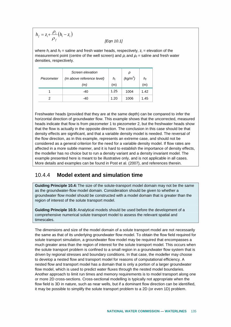
inverse of hydraulic resistance is the hydraulic conductance

152 Solute transport

Solutes in groundwater are generally transported by flow This process is termed advection (or

sometimes convection) Besides being carried by groundwater flow solutes move from regions

of high solute concentration to regions of low solute concentration in a process known as

diffusion Even if there is no groundwater flow solutes are transported through a groundwater

system if spatial concentration differences exist

The quantitative expressions of groundwater flow and solute transport processes are for all

practical purposes macroscopiclsquo descriptions That is they describe the overall direction and rate of movement of a parcel of groundwater and the solutes contained therein but they do not

resolve the complex flow paths at the microscopic scale The spreading of solutes that occurs

due to microscopic flow variations is called dispersion Dispersion also occurs due to the spatial

variability of the hydraulic properties of the subsurface The hydraulic conductivity

representation in models is an approximation of the truelsquo hydraulic conductivity distribution and thus the model does not directly capture all of the solute spreading that occurs in reality

Dispersion and diffusion cause solute spreading both parallel and perpendicular to the flow

direction

Solute concentrations can also change as a result of interaction with other solutes with aquifer

material through degradation or decay and through mass transfer between the four commonly

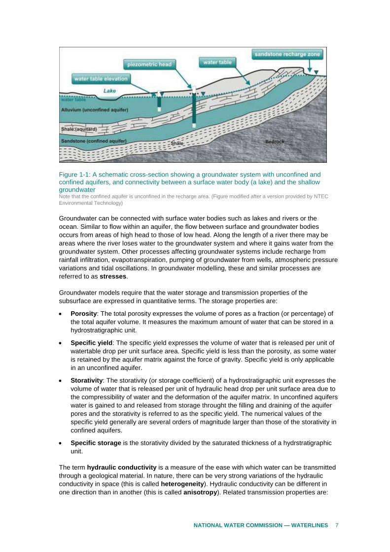
described phases (dissolved vapour sorbed (solid) and liquid (separate))

Groundwater flow can be affected where significant spatial variation in solute concentration

andor temperature causes significant groundwater density variations Examples include coastal

aquifers or deep aquifers containing waters of elevated temperature like those in the Great

Artesian Basin In some instances groundwater flow can be driven purely by density

differences such as underneath salt lakes where strong evaporation at the surface results in an

unstable density stratification

153 Common simplifications

In nature groundwater flow patterns are complex and continuously change with time but for

the purposes of modelling simplifications are required

One important consideration in the description of flow processes relates to the temporal

variability of the flow A system is said to be in a steady state when the flow processes are (at

least to a good approximation) constant with time The inflows to and the outflows from the

system are equal and as a result there is no change in storage within the aquifer This also

means that the heads and watertable elevation do not change with time When the inflows term

and outflows term differ the total amount of water in the system under consideration changes

the heads and watertable elevation are changing with time and the system is described as being

in an unsteady or transient state


Simplifying assumptions regarding the direction of flow in aquifers and aquitards are often made

to reduce the complexity for the purposes of mathematical analysis of the flow problem (both for

steady state and unsteady state systems) One of these is that the flow in the aquifer is strictly

horizontal and that flow in aquitards is vertical These assumptions are based on the

observation that horizontal head gradients in aquifers are usually much greater than vertical

gradients and that the flow through aquitards tends to be along the shortest possible flow path

The use of this simplifying assumption has led to a method known as the quasi 3D approach in

groundwater modelling It is suited for the description of regional flow when the hydraulic

conductivities of aquifers and aquitards differ by a factor of 100 or more It must be used with

caution for local scale problems or where the thickness of the aquifer is substantial and

resolution of the vertical flow and vertical hydraulic gradients is required Alternative modelling

methods that allow vertical flow in aquifers through the use of multiple aquifer model layers and

the explicit representation of the aquitards are also commonly used and can be considered as a

fully 3D approach

154 Flow and solute transport modelling

The fundamental relationships governing groundwater flow and solute transport are based on

the principle of mass conservation for an elementary control volume the change in storage of

water or solute mass within the volume equals the difference between the mass inflow and

outflow This principle can be expressed in mathematical terms and combined with the empirical

laws that govern the flow of water and solutes in the form of differential equations The resulting

differential equations can be solved in two ways

Using techniques of calculus The resulting analytical models are an exact solution of the

governing differential equation Many simplifying assumptions are needed to obtain an

analytical solution For example the decline in groundwater level can be determined at a

given distance from a single fully penetrating well pumping at a constant rate in a

homogeneous aquifer of constant thickness Analytical models exist for a wide range of

hydrogeological problems Natural systems incorporate complexities that depending on the

scale of the study may violate the simplifying assumptions of analytical models Examples

include spatial variation of hydraulic or transport properties complex geometry associated

with rivers or coastlines spatial and temporal recharge and evapotranspiration variability

Using numerical techniques In numerical models space and time are subdivided into

discrete intervals and the governing differential equations are replaced by piecewise

approximations Heads and solute concentrations are calculated at a number of discrete

points (nodes) within the model domain at specified times Numerical models are used when

spatial heterogeneity andor temporal detail are required to adequately describe the

processes and features of a hydrogeological system

In both cases conditions at the model boundaries and for time-dependent problems at the start

of the simulation need to be defined to solve the differential equations This is done by

specifying boundary conditions for heads andor fluxes and initial conditions for heads (andor

solute concentrations) The combination of the governing equations the boundary and initial

conditions and the definition of hydrogeological parameters required to solve the groundwater

flow and solute transport equations is what is referred to as the mathematical model

Analytical models are usually solved quickly but require more simplifying assumptions about the

groundwater system Numerical models enable more detailed representation of groundwater

systems but typically take longer to construct and solve Analytic element models are a

category of models that superimpose analytic expressions for a number of hydrologic features

and thus provide increased flexibility compared to analytical solutions of single features

However they are still not as versatile as numerical models Analytical and numerical models

can each be beneficial depending on the objectives of a particular project


Most of the information included in these guidelines relates to numerical groundwater models

There are two primary reasons for this emphasis

First the use of numerical modelling in the groundwater industry has been expanding more

rapidly than the use of analytical techniques This has largely been brought about by

increased computational power solution techniques for the non-linear partial differential

equations and the development of user-friendly modelling software

Second the level of system complexity that can be considered in a numerical model

exceeds that of analytical and analytic element models Therefore more detailed discussion

is required to adequately cover numerical models

155 Uncertainty associated with model predictions

Model predictions are uncertain because models are built on information constraints and

because the capacity to capture real-world complexity in a model is limited

In many cases results from models are presented in a way that suggests there is one right

answer provided by the model such as the presentation of a single set of head contours or

hydrographs for a particular prediction However it is more useful (and correct) to show that all

model predictions contain uncertainty and that given the available data there is a distribution or

range of plausible outputs that should be considered for each model prediction

Open and clear reporting of uncertainty provides the decision-maker with the capacity to place

model outputs in the context of risk to the overall project objectives

Uncertainty can be handled in different ways A manager may accept the level of prediction

uncertainty that is estimated and make decisions that reflect an acceptable level of risk

stemming from that uncertainty It may be possible to reduce the level of uncertainty by

gathering more data or taking a different modelling approach

Example 1A Handling uncertainty

Uncertainty is commonly handled in everyday life such as with concepts of probability used in

weather forecasts Another common approach to handling uncertainty is an engineering safety

factor For example the parameter hydraulic conductivity is intrinsically variable and has some

scale dependence in the natural world Therefore exact predictions of how much a pump will

discharge is uncertain Yet a decision on what size pipe is needed to convey the pumplsquos discharge is decided in the context of well-defined thresholds that are set by manufacturing

standards Therefore in cases where the capacity of a standard pipe may be exceeded the

intrinsic uncertainty of the pump discharge can be handled by incurring slightly larger costs with

use of a larger pipe diameter Such a safety factor approach will likely be more effective and

cost-efficient than detailed characterisation of the sediments around the well screen and

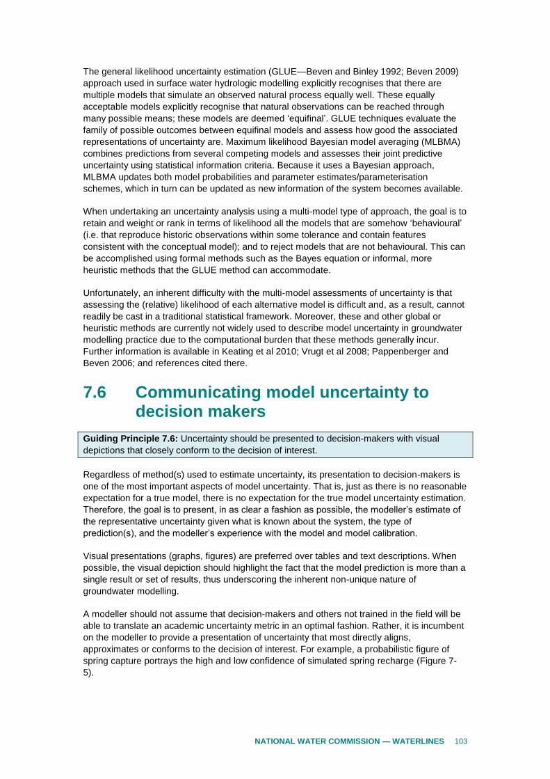
sophisticated uncertainty analyses However if the goal of the analysis is to protect a public

water supply effective and cost-efficient hydraulic capture of a contaminant plume using

pumping wells requires a more detailed uncertainty analysis to ensure that the system functions

as intended and the public protected

A discussion of concepts and approaches for estimation of uncertainty associated with model

predictions is provided in Chapter 7 While the description of uncertainty analysis is presented in

these guidelines as a single chapter the models most suited for decision-making are those that

address the underlying sources of uncertainty and the effect of model simplifications on

uncertainty throughout the entire modelling process


Potential sources of uncertainty can be assessed during conceptualisation once the modelling

objectives predictions and intended use(s) of the model have been agreed The complexity in

the groundwater system is characterised during conceptualisation and decisions are made on

how to simplify the representation of the system prior to model design and construction

Different sources of uncertainty are explored further during parameterisation and calibration

Parameter distributions (and other model inputs) are characterised at this stage possibly for

multiple conceptual models and designs

Once the predictive modelling stage is reached the modelling team will have a view of how the

potential sources of uncertainty will influence the predictions This view can be supported by

qualitative or quantitative assessments of uncertainty as described in Chapter 7

The level of effort applied to uncertainty analysis is a decision that is a function of the risk being

managed A limited analysis such as an heuristic assessment with relative rankings of

prediction uncertainty or through use of the confidence-level classification as described in

section 25 may be sufficient where consequences are judged to be lower More detailed and

robust analysis (eg those based on statistical theory) is advisable where consequences of

decisions informed by model predictions are greater Because uncertainty is an integral part of

any model it is recommended to consider early in the modelling project the level of effort

required for uncertainty analysis the presentation of results and the resources required

16 The modelling process

The groundwater modelling process has a number of stages As a result the modelling team

needs to have a combination of skills and at least a broad or general knowledge of

hydrogeology the processes of groundwater flow the mathematical equations that describe

groundwater flow and solute movement analytical and numerical techniques for solving these

equations and the methods for checking and testing the reliability of models

The modellerlsquos task is to make use of these skills provide advice on the appropriate modelling

approach and to blend each discipline into a product that makes the best use of the available

data time and budget In practice the adequacy of a groundwater model is best judged by the

ability of the model to meet the agreed modelling objectives with the required level of

confidence The modelling process can be subdivided into seven stages (shown schematically

in Figure 1-2) with three hold points where outputs are documented and reviewed

The process starts with planning which focuses on gaining clarity on the intended use of the

model the questions at hand the modelling objectives and the type of model needed to meet

the project objectives The next stage involves using all available data and knowledge of the

region of interest to develop the conceptual model (conceptualisation) which is a description

of the known physical features and the groundwater flow processes within the area of interest

The next stage is design which is the process of deciding how to best represent the conceptual

model in a mathematical model It is recommended to produce a report at this point in the

process and have it reviewed Model construction is the implementation of model design by

defining the inputs for the selected modelling tool

The calibration and sensitivity analysis of the model occurs through a process of matching

model outputs to a historical record of observed data It is recommended that a calibration and

sensitivity analysis report be prepared and reviewed at this point in the process The guidelines

recognise that in some cases model calibration is not necessary for example when using a

model to test a conceptual model


Predictions comprise those model simulations that provide the outputs to address the

questions defined in the modelling objectives The predictive analysis is followed by an analysis

of the implications of the uncertainty (refer section 15) associated with the modelling outputs

Clear communication of the model development and quality of outputs through model reporting

and review allows stakeholders and reviewers to follow the process and assess whether the

model is fit for its purpose that is meets the modelling objectives

The process is one of continual iteration and review through a series of stages For example

there is often a need to revisit the conceptual model during the subsequent stages in the

process There might also be a need to revisit the modelling objectives and more particularly

reconsider the type of model that is desired once calibration has been completed Any number

of iterations may be required before the stated modelling objectives are met Accordingly it is

judicious at the planning stage to confirm the iterative nature of the modelling process so that

clients and key stakeholders are receptive to and accepting of the approach

While the reviewer has primary responsibility for judging whether or not a stage of modelling

work has been completed to an adequatelsquo standard (and move to the next stage) there is a need to involve the modelling team and model owner in this discussion


YES

STAGE 1 Planning

DATA AND GAP

ANALYSIS

CONCEPTUALISATION

AND DESIGN REPORT

AND REVIEW

STAGE 2

Conceptualisation

STAGE 5 Calibration

and Sensitivity Analysis

STAGE 6 Prediction

STAGE 7 Uncertainty

Analysis

FINAL REPORT AND

REVIEW

STAGE 8 Final

Reporting and Archiving

CALIBRATION AND

SENSITIVITY REPORT

AND REVIEW

YES

NO

YES

STAGE 4 Construction

STAGE 3 Design

Adequate

The feedback loops allow

the process to go back to

any one of the proceeding

stages as required

For example the reviewer

may judge the model

design to be inadequate

which can mean revisiting

the conceptual model or

the planning stage

NO Adequate

NO Adequate

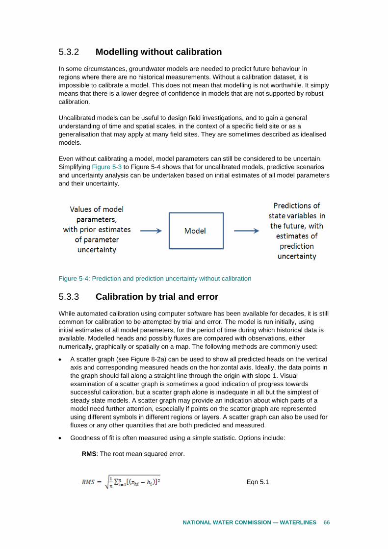
Figure 1-2 Groundwater modelling process (modified after MDBC 2001 and Yan et al 2010)


2 Planning In this chapter

Introduction

Intended use of the model

Defining modelling objectives

Initial consideration of investigation scale

Model confidence-level classification

Defining exclusions

Review and update

Model ownership

Guiding principles for planning a groundwater model

Guiding Principle 21 Modelling objectives should be prepared early in a modelling project as

a statement of how the model can specifically contribute to the successful completion or

progress of the overall project

Guiding Principle 22 The modelling objectives should be used regularly throughout the

modelling process as a guide to how the model should be conceptualised designed calibrated

and used for prediction and uncertainty analysis

Guiding Principle 23 A target model confidence-level classification should be agreed and

documented at an early stage of the project to help clarify expectations The classification can

be estimated from a semi-quantitative assessment of the available data on which the model is

based (both for conceptualisation and calibration) the manner in which the model is calibrated

and how the predictions are formulated

Guiding Principle 24 The initial assessment of the confidence-level classification should be

revisited at later stages of the project as many of the issues that influence the classification will

not be known at the model planning stage

21 Introduction

This chapter outlines the key issues that need consideration at the planning stage of a project

such as how the model will be used the modelling objectives and the type of model to be

developed (eg simple analytical or numerical flow only or flow and solute transport) In general

terms the planning process seeks to determine what is achievable and what is required


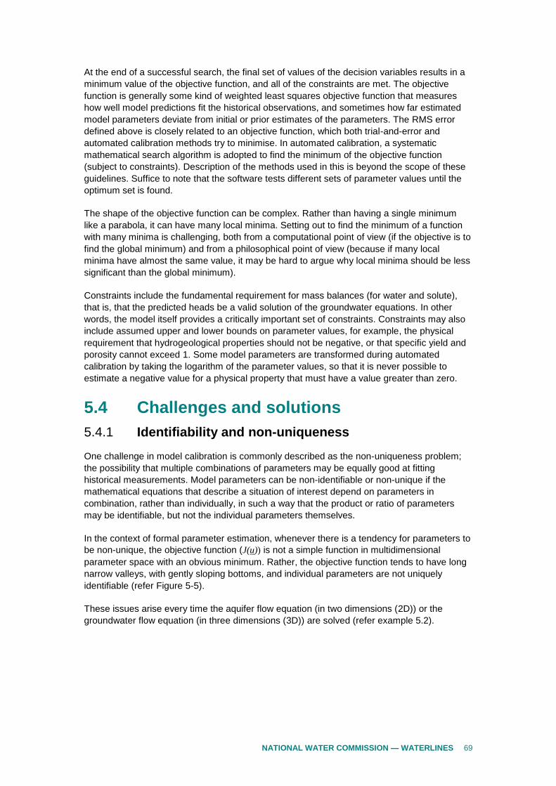
Fi gure 2-1 The planning process

Planning seeks alignment of expectations of the modelling team the model owner and other key

stakeholders It provides the basis for a subsequent judgement on whether the model products

that are created (eg conceptualisation calibrated model predictions) are fit for purpose To this

end the concept of a model confidence level classification is introduced which provides a

means of ranking the relative confidence with which a model can be used in predictive mode At

the planning stage it is recommended that agreement be made on a target confidence level

classification (refer to section 25) based on the objectives and requirements of the project as

well as on the available knowledge base and data from which the model can be developed

22 Intended use of the model

It is never possible for one model to answer all questions on groundwater behaviour For

example a model designed to simulate regional-scale groundwater flow cannot be expected to

predict local-scale groundwater processes (eg groundwater interaction with one stream

meander loop) Similarly a local-scale model of impacts of pumping at a single well cannot be

extrapolated to predict the drawdown due to development of an extensive borefield in a

heterogeneous aquifer In the planning stage at the outset of a modelling project it is necessary

to clearly understand the intended use of the model so that it can be designed constructed and

calibrated to meet the particular requirements of the problem at hand

The modelling team must consider how the model will be used The discussion of the intended

use of the model must include not only the final products sought but also confirmation of the

specific modelling features that will be used to provide the desired outcomes as this will affect

how the model will be designed and calibrated It may also consider the manner in which the

required outcomes will be obtained from model results including additional data processing that

may be needed to convert the model predictions into a form that can illustrate the particular

behaviour of interest

Example 21 How the intended use of the model influences model calibration and data

requirements

If a model is required to predict the future impacts of groundwater extraction on river base flow

with a high level of confidence the calibration should include a comparison of calculated

groundwater fluxes into the river with measured or estimated fluxes (eg as inferred from base-

flow analysis)

In some cases the intended model uses may change as a project progresses or after it has

been completed For example a groundwater flow model may initially be developed to

investigate regional water resource management issues It may subsequently be used as the

basis for a solute transport model to investigate water quality issues


In describing the intended model uses it is appropriate to also provide or consider the

justification for developing a model as opposed to choosing alternative options to address the

question at hand In this regard it may be necessary to consider the cost and risk of applying

alternative methods

At this time it is also worth reviewing the historical and geographical context within which the

model is to be developed A thorough review and reference to previous or planned models of

the area or neighbouring areas is appropriate

23 Defining modelling objectives


a statement of how the model will specifically contribute to the successful completion or





The modelling objectives

establish the context and framework within which the model development is being

undertaken

guide how the model will be designed calibrated and run

provide criteria for assessing whether the model is fit for purpose and whether it has yielded

the answers to the questions it was designed to address

In general a groundwater model will be developed to assist with or provide input to a larger

project (eg an underground construction project a groundwater resource assessment or a

mining feasibility study) Models are developed to provide specific information required by the

broader project and will usually represent one aspect of the overall work program undertaken for

a particular project

Often the objectives will involve the quantitative assessment of the response of heads flows or

solute concentrations to future stresses on the aquifer system However in some cases the

objective may not be to quantify a future response Rather it may be to gain insight into the

processes that are important under certain conditions to identify knowledge gaps and inform

where additional effort should be focused to gather further information

24 Initial consideration of investigation scale

It is necessary to initially define the spatial and temporal scales considered to be important

within the overall project scope The spatial scale depends on the extent of the groundwater

system of interest the location of potential receptors (eg a groundwater dependent ecosystem)

or the extent of anticipated impacts The timescale of interest may relate to planning or

development time frames system response time frames (including system recovery such as

water-level rebound after mine closure) or impacts on water resources by decadal-scale

changes in recharge Further and more detailed consideration of model scale and extent occurs

during the conceptualisation stage (refer Chapter 3) and is confirmed in the design stage of the

project (refer Chapter 4)


25 Model confidence level classification

Guiding Principle 23 A target model confidence level classification should be agreed and





Guiding Principle 24 The initial assessment of the confidence level classification should be



Because of the diverse backgrounds and make-up of the key stakeholders in a typical modelling

project it is necessary to define in non-technical terms a benchmark or yardstick by which the

reliability or confidence of the required model predictions can be assessed The guidelines

recommend adoption of confidence level classification terminology

The degree of confidence with which a modellsquos predictions can be used is a critical consideration in the development of any groundwater model The confidence level classification

of a model is often constrained by the available data and the time and budget allocated for the

work While model owners and other stakeholders may be keen to develop a high-confidence

model this may not be practicable due to these constraints The modeller should provide advice

(based on experience) on realistic expectations of what level of confidence can be achieved

Agreement and documentation of a target confidence level classification allow the model owner

modellers reviewers and other key stakeholders to have realistic and agreed expectations for

the model It is particularly important for a model reviewer to be aware of the agreed target

model confidence level classification so that it is possible to assess whether or not the model

has met this target

In most circumstances a confidence level classification is assigned to a model as a whole In

some cases it is also necessary to assign confidence-level classifications to individual model

predictions as the classification may vary depending on how each prediction is configured (eg

the level of stress and the model time frame in comparison to those used in calibration)

Factors that should be considered in establishing the model confidence-level classification

(Class 1 Class 2 or Class 3 in order of increasing confidence) are presented in Table 2-1 Many

of these factors are unknown at the time of model planning and as such the guidelines

recommend reassessing the model confidence-level classification regularly throughout the

course of a modelling project The level of confidence typically depends on

the available data (and the accuracy of that data) for the conceptualisation design and

construction Consideration should be given to the spatial and temporal coverage of the

available datasets and whether or not these are sufficient to fully characterise the aquifer

and the historic groundwater behaviour that may be useful in model calibration

the calibration procedures that are undertaken during model development Factors of

importance include the types and quality of data that is incorporated in the calibration the

level of fidelity with which the model is able to reproduce observations and the currency of

calibration that is whether it can be demonstrated that the model is able to adequately

represent present-day groundwater conditions This is important if the model predictions are

to be run from the present day forward


the consistency between the calibration and predictive analysis Models of high

confidence level classification (Class 3 models) should be used in prediction in a manner

that is consistent with their calibration For example a model that is calibrated in steady

state only will likely produce transient predictions of low confidence Conversely when a

transient calibration is undertaken the model may be expected to have a high level of

confidence when the time frame of the predictive model is of less or similar to that of the

calibration model

the level of stresses applied in predictive models When a predictive model includes

stresses that are well outside the range of stresses included in calibration the reliability of

the predictions will be low and the model confidence level classification will also be low

Table 2-1 provides a set of quantifiable indicators from which to assess whether the desired

confidence-level classification has been achieved (ie fit for purpose)

In many cases a Class 1 model is developed where there is insufficient data to support

conceptualisation and calibration when in fact the project is of sufficient importance that a

Class 2 or 3 model is desired In these situations the Class 1 model is often used to provide an

initial assessment of the problem and it is subsequently refined and improved to higher classes

as additional data is gathered (often from a monitoring campaign that illustrates groundwater

response to a development)

In some circumstances Class 1 or Class 2 confidence-level classification will provide sufficient

rigour and accuracy for a particular modelling objective irrespective of the available data and

level of calibration In such cases documentation of an agreement to target a Class 1 or 2

confidence level classification is important as the model can be considered fit for purpose even

when it is rated as having a relatively low confidence associated with its predictions At this point

it is worth noting that there is a strong correlation between the model confidence-level

classification and the level of resources (modelling effort and budget) required to meet the target

classification Accordingly it is expected that lower target-level classifications may be attractive

where available modelling time and budgets are limited

The model confidence-level classification provides a useful indication of the type of modelling

applications for which a particular model should be used Table 2-1 includes advice on the

appropriate uses for the three classes of model A Class 1 model for example has relatively

low confidence associated with any predictions and is therefore best suited for managing low-

value resources (ie few groundwater users with few or low-value groundwater dependent

ecosystems) for assessing impacts of low-risk developments or when the modelling objectives

are relatively modest The Class 1 model may also be appropriate for providing insight into

processes of importance in particular settings and conditions Class 2 and 3 models are suitable

for assessing higher risk developments in higher-value aquifers

It is not expected that any individual model will have all the defining characteristics of Class 1 2

or 3 models The characteristics described in Table 2-1 are typical features that may have a

bearing on the confidence with which a model can be used A model can fall into different

classes for the various characteristics and criteria included in Table 2-1


It is up to the modelling team and key stakeholders to agree on which of these criteria are most

relevant for the model and project at hand and to agree on an overall confidence-level

classification that reflects the particular requirements and features of that model In general it

should be acknowledged that if a model has any of the characteristics or indicators of a Class 1

model it should not be ranked as a Class 3 model irrespective of all other considerations It may

also be appropriate to provide classifications for each of the three broad sectors included in

Table 2-1 (ie data calibration and prediction) based on all characteristics and criteria for that

sector An overall model classification can be chosen that reflects the importance of the

individual criteria and characteristics with regard to the model and project objectives If a model

falls into a Class 1 classification for either the data calibration or prediction sectors it should be

given a Class 1 model irrespective of all other ratings

When considering the confidence level classification there is a class of model commonly

referred to as a generic modellsquo that is worthy of special consideration These models are

developed primarily to understand flow processes and not to provide quantitative outcomes for

any particular aquifer or physical location They can be considered to provide a high level of

confidence as their accuracy is only limited by the ability of the governing equations to replicate

the physical processes of interest While they provide high confidence when applied in a

general non-specific sense if the results are applied to or assumed to represent a specific site

the confidence level will automatically decrease This is because the simplifying assumptions

(eg the aquifer geometry) implemented in the generic model are highly unlikely to be exactly

applicable to the real physical setting

Example 22 Generic groundwater flow model

Consider a groundwater flow model developed to calculate the relationship between

groundwater extraction location and the associated impact on base flow in a nearby river The

model may be developed by a regulator in order to help define rules that constrain the location

of groundwater extraction in relation to a river to help minimise impacts on river flow It is

intended that the results will be applied to all rivers and aquifers in the jurisdiction The model is

required to assess the phenomena generally within a wide spectrum of aquifer conditions and

geometries and is classed as a generic modellsquo

A target confidence-level classification for the model should be defined at the outset as

subsequent project stages such as the conceptualisation (refer Chapter 3) design (refer

Chapter 4) calibration (refer Chapter 5) and predictive scenario development (refer Chapter 6)

are influenced by the confidence-level classification As the model development progresses the

model confidence-level classification should be reassessed to determine whether the targeted

classification has or can be achieved and if necessary whether the target classification can be

revised At the completion of the modelling project it is expected that the model reviewer will

assess whether the final model meets the key criteria that define the stated level of confidence

classification


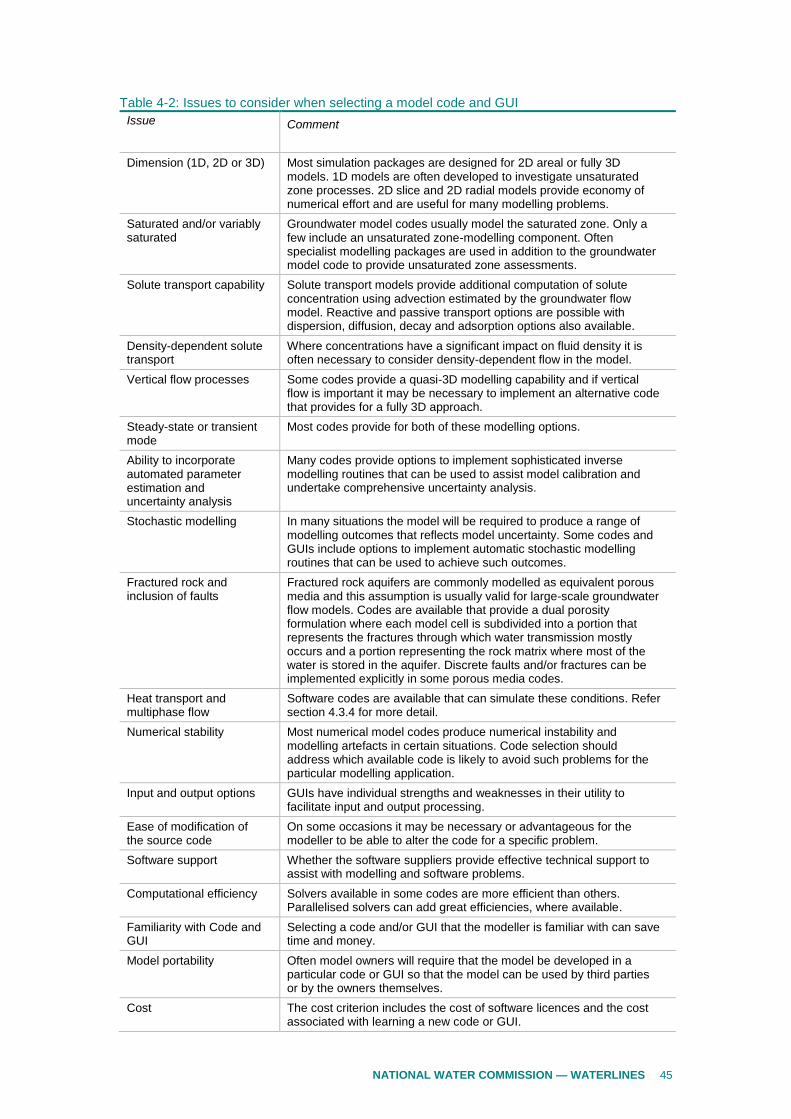
Table 2-1 Model confidence level classificationmdashcharacteristics and indicators

Confidence level

classification Data Calibration Prediction Key indicator Examples of specific

uses

Class 3 Spatial and temporal distribution of groundwater head observations adequately define groundwater behaviour especially in areas of greatest interest and where outcomes are to be reported

Spatial distribution of bore logs and associated stratigraphic interpretations clearly define aquifer geometry

Reliable metered groundwater extraction and injection data is available

Rainfall and evaporation data

Adequate validation is demonstrated

Scaled RMS error (refer Chapter 5) or other calibration statistics are acceptable

Long-term trends are adequately replicated where these are important

Seasonal fluctuations are adequately replicated where these are important

Transient calibration is current ie uses recent data

Length of predictive model is not excessive compared to length of calibration period

Temporal discretisation used in the predictive model is consistent with the transient calibration

Level and type of stresses included in the predictive model are within the range of those used in the transient calibration

Model validation suggests calibration is appropriate for locations

Key calibration statistics are acceptable and meet agreed targets

Model predictive time frame is less than 3 times the duration of transient calibration

Stresses are not more than 2 times greater than those included in calibration

Temporal discretisation in predictive model is the same as that used in calibration

Mass balance closure error is less than 05 of total

Model parameters consistent with conceptualisation

Suitable for predicting groundwater responses to arbitrary changes in applied stress or hydrological conditions anywhere within the model domain

Provide information for sustainable yield assessments for high-value regional aquifer systems

Evaluation and management of potentially high-risk impacts

Can be used to design is available

Aquifer-testing data to define key parameters

Streamflow and stage measurements are available with reliable baseflow estimates at a number of

Model is calibrated to heads and fluxes

Observations of the key modelling outcomes dataset is used in calibration

andor times outside the calibration model

Steady-state predictions used when the model is calibrated in steady-state only

Appropriate computational methods used with appropriate spatial discretisation to model the problem

The model has been reviewed and deemed fit for purpose by an experienced independent

complex mineshydewatering schemes salt-interception schemes or water-allocation plans

Simulating the interaction between

points

Reliable land-use and soil-mapping data available

Reliable irrigation application data (where relevant) is available

Good quality and adequate spatial coverage of digital elevation model to define ground surface elevation

hydrogeologist with modelling experience

groundwater and surface water bodies to a level of reliability required for dynamic linkage to surface water models

Assessment of complex large-scale solute transport processes

Class 2 Groundwater head Validation is either not Transient calibration Key calibration statistics suggest Prediction of impacts of observations and bore logs undertaken or is not over a short time frame poor calibration in parts of the proposed developments are available but may not demonstrated for the full compared to that of model domain in medium value provide adequate coverage model domain prediction Model predictive time frame is aquifers throughout the model Calibration statistics are Temporal discretisation between 3 and 10 times the Evaluation and domain generally reasonable but used in the predictive duration of transient calibration management of medium

Contrsquod overleaf may suggest significant model is different from Stresses are between 2 and 5 risk impacts errors in parts of the that used in transient times greater than those


Confidence level


uses

Class 2 Contrsquod Metered groundwater-extraction data may be available but spatial and temporal coverage may not be extensive

Streamflow data and baseflow estimates available at a few points

Reliable irrigation-application data available in part of the area or for part of the model duration

model domain(s)

Long-term trends not replicated in all parts of the model domain

Transient calibration to historic data but not extending to the present day

Seasonal fluctuations not adequately replicated in all parts of the model domain

Observations of the key modelling outcome data set are not used in calibration

calibration

Level and type of stresses included in the predictive model are outside the range of those used in the transient calibration

Validation suggests relatively poor match to observations when calibration data is extended in time andor space

included in calibration

Temporal discretisation in predictive model is not the same as that used in calibration


Not all model parameters consistent with conceptualisation

Spatial refinement too coarse in key parts of the model domain

The model has been reviewed and deemed fit for purpose by an independent hydrogeologist

Providing estimates of dewatering requirements for mines and excavations and the associated impacts

Designing groundwater management schemes such as managed aquifer recharge salinity management schemes and infiltration basins

Estimating distance of travel of contamination through particle-tracking methods Defining water source protection zones

Class 1 Few or poorly distributed existing wells from which to obtain reliable groundwater and geological information

Observations and measurements unavailable or sparsely distributed in areas of greatest interest

No available records of metered groundwater extraction or injection

Climate data only available from relatively remote locations

Little or no useful data on land-use soils or river flows and stage elevations

No calibration is possible

Calibration illustrates unacceptable levels of error especially in key areas

Calibration is based on an inadequate distribution of data

Calibration only to datasets other than that required for prediction

Predictive model time frame far exceeds that of calibration

Temporal discretisation is different to that of calibration

Transient predictions are made when calibration is in steady state only

Model validation suggests unacceptable errors when calibration dataset is extended in time andor space

Model is uncalibrated or key calibration statistics do not meet agreed targets

Model predictive time frame is more than 10 times longer than transient calibration period

Stresses in predictions are more than 5 times higher than those in calibration

Stress period or calculation interval is different from that used in calibration

Transient predictions made but calibration in steady state only

Cumulative mass-balance closure error exceeds 1 or exceeds 5 at any given calculation time

Model parameters outside the range expected by the conceptualisation with no further justification

Unsuitable spatial or temporal discretisation

The model has not been reviewed

Design observation bore array for pumping tests

Predicting long-term impacts of proposed developments in low-value aquifers

Estimating impacts of low-risk developments

Understanding groundwater flow processes under various hypothetical conditions

Provide first-pass estimates of extraction volumes and rates required for mine dewatering

Developing coarse relationships between groundwater extraction locations and rates and associated impacts

As a starting point on which to develop higher class models as more data is collected and used

(Refer Chapter 5 for discussion around validation as part of the calibration process)


Example 23 Project objectives and modelling objectives related to intended use and

confidence level classification

Water resource management model

Project objective To determine the maximum sustainable extraction from an aquifer

Intended use Model outcomes will assist resource managers determine appropriate

volumetric extraction rates

Modelling objective To provide quantitative estimates of drawdown loss of baseflow and

reduction in water availability to groundwater dependent ecosystems for various levels of

groundwater extraction and future climate assumptions

Target confidence level Class 3 in keeping with the availability of extensive groundwater

data within the area of interest

Mine-dewatering model

Project objective To design a dewatering scheme for a planned mine

Intended use To estimate the drawdown caused by an array of dewatering wells

Modelling objective To determine optimum groundwater pumping (including the rate the

number of bores and their location) required to dewater an open-pit mine

Target confidence level Class 1ndash-2 level of confidence due to a lack of useful time series

data that can be used for calibration The level of confidence is expected to increase once

mining starts and model validation can be undertaken

Tunnel construction and operation

Project objective To assess the environmental impacts of tunnel construction and operation

Intended use Predict drawdown and associated loss of baseflow arising from inflows to the

tunnel

Modelling objective To provide quantitative estimates of the groundwater inflows and

associated drawdown during the construction and operation of a new tunnel

Target confidence level Class 2 as the available data only allows for a steady state

calibration

26 Defining exclusions

In this section the term modelling exclusionslsquo refers to specific elements of the model that for

any reason should not be used to generate or report predictive outcomes In the course of

the modelling process it may be found that specific features or areas of the model have a

particularly low level of confidence This may arise for example when the particular

application or model area has insufficient reliable data on which to base calibration when the

model code may be unsuitable for a particular application or when the model was not

developed for that purpose and hence outcomes are likely to be unreliable In such cases it

should be noted that certain model outputs are likely to be particularly uncertain and hence

should not be relied upon The modellers should provide an explicit statement of exclusions to

help avoid inappropriate model use in the current project or any future projects that make use

of the model


Although model exclusions may first be identified at the initial planning stage they will also be

defined and confirmed during the course of model development and calibration Often the

modelling exclusions will be accumulated and reported at the completion of the project within

a modelling limitations section of the final modelling report Chapter 8 provides more details

on reporting


Basement layers Depressurisation of an aquifer in response to pumping can trigger the

release of water from underlying strata into the pumped aquifer These underlying layers can

be explicitly considered in the model to simulate this process However often there is no data

available in these strata that can be used for calibration purposes Hence little or no

confidence must be placed on the specific responses predicted in this part of the model

Aquitards Aquitards present in a model domain are often represented in a groundwater

model as a single model layer with appropriately chosen parameters to reflect their poor

transmission characteristics This configuration does not adequately resolve the vertical

hydraulic head distribution across the aquitard In this case it may not be appropriate to report

the predicted groundwater responses in the aquitard (refer to section 444)

27 Review and update

In many modelling projects the conceptualisation calibration and predictive analysis will be

updated and revised as more information becomes available and as modelling results

illustrate the need for such revisions It may be necessary to revise expectations of the

confidence levels associated with the model outputs This may be required if for example

model calibration is more difficult than expected and the final calibrated model is less

constrained than originally envisaged Conversely an upgrade in model confidence-level

classification is also possible when additional data is obtained that leads to an improvement in

the calibration of model parameters

In some cases the modelling objectives themselves will need to be revised or updated This is

rarely required if the overall project objectives remain unchanged but may be appropriate if

the model is required to address additional issues that may arise during the course of the

project or when an existing model is applied in a new project

28 Model ownership

The planning stage is an appropriate time for the modeller and model owner to agree on a

number of issues about the future ownership and ongoing maintenance of the model An

agreement on intellectual property is a key aspect that should be understood by both parties

at the outset The discussion should extend to agreement on how the model will be archived

including the data-file formats the physical location of where model files will be stored long-

term custodianship and third-party access to the model More information on model archiving

can be found in section 86


3 Conceptualisation In this chapter

Introduction

The principle of simplicity

Conceptualisation of current and future states

Alternative conceptual models

Data collection analysis and data checking

Developing the conceptual model

Checking the conceptual model

3D visualisation

Conceptualisation as an ongoing process

Reporting and review

Guiding principles for conceptualisation

Guiding Principle 31 The level of detail within the conceptual model should be chosen

based on the modelling objectives the availability of quality data knowledge of the

groundwater system of interest and its complexity

Guiding Principle 32 Alternative conceptual models should be considered to explore the

significance of the uncertainty associated with different views of how the system operates

Guiding Principle 33 The conceptual model should be developed based on observation

measurement and interpretation wherever possible Quality-assured data should be used to

improve confidence in the conceptual model

Guiding Principle 34 The hydrogeological domain should be conceptualised to be large

enough to cover the location of the key stresses on the groundwater system (both the current

locations and those in the foreseeable future) and the area influenced or impacted by those

stresses It should also be large enough to adequately capture the processes controlling

groundwater behaviour in the study area

Guiding Principle 35 There should be an ongoing process of refinement and feedback

between conceptualisation model design and model calibration to allow revisions and

refinements to the conceptual model over time

31 Introduction

Conceptualisation is a process that provides the basis for model design and communicates

how the system works to a wide range of audiences The conceptual model should be

developed collaboratively across relevant disciplines and project stakeholders

A conceptual (hydrogeological) model is a descriptive representation of a groundwater system

that incorporates an interpretation of the geological and hydrological conditions (Anderson

and Woessner 1992) It consolidates the current understanding of the key processes of the

groundwater system including the influence of stresses and assists in the understanding of

possible future changes


This chapter outlines the process of developing a conceptual model as a prelude to designing

and constructing a model of the groundwater system which broadly involves using all existing

information to create an understanding of how the system operates (Figure 3-1)

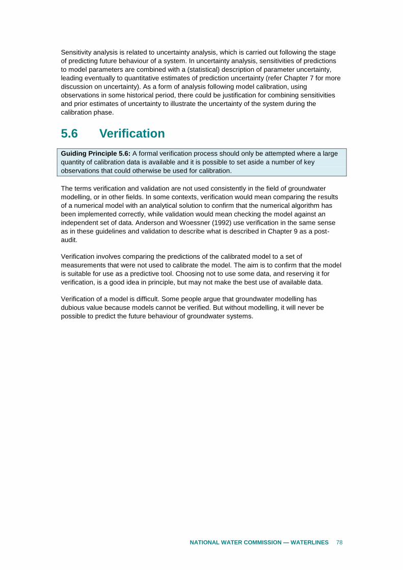
Figure 3-1 Creating a conceptual model

The development of the most appropriate conceptual model is required to ensure that the

model activity achieves its objectives The conceptual model development process may need

to include people with a range of skills (modelling hydrogeology climate environmental

systems etc) and represents a key point in the modelling process where a decision to

proceed past the conceptual stage is required It may be the case that it is not possible to

proceed in the current format given the state of knowledge of the groundwater system Some

project re-scoping and redesign may also need to occur irrespective of a decision to proceed

The following sections provide a series of suggestions about the issues that can arise during

the conceptualisation process Conceptualisation has the potential to embed structural

problems in a model from the outset if poor decisions are mademdashproblems that cannot be

removed through later parameter optimisation during the calibration stage If a model is

conceptually poor no amount of calibration can fix it This is the primary reason for paying

strict attention to the conceptualisation process and why it is fundamental to the entire

modelling process that the conceptualisation is as close to correctlsquo as possible recognising that it is difficult to understand what correctlsquo looks like (refers Box 3B on conceptual surprise)

The guidance below provides some suggestions to enable the project to iterate towards this

correctlsquo conceptual model

32 The principle of simplicity




When developing conceptual models there is always a trade-off between realism generality

and precision it is not possible to maximise all three simultaneously (Levins 1966) The

conceptualisation process involves simplifying a groundwater system which is inherently

complex in order to simulate the systemlsquos key behaviour This is the principle of simplicity

Levinslsquos original ideas were developed for population biology models and there are

suggestions that they may not equally apply to the more deterministic sciences This issue is

not relevant to this discussion rather it is the general principle of having to trade off to some

degree in the conceptualisation process or in a more general manner to be aware that tradeshy

offs may be required This has been more generally popularised as less is morelsquo and

provides a good philosophy for hydrogeological conceptualisations


There is no perfect way to simplify a system within a conceptualisation The only issue is

whether the model suffices for the task it is expected to address Which aspects of the

groundwater system should be considered in simplification and to what level of detail is

dictated by

the objectives of the study for which the model is being developed and the target

confidence level classification of the model (refer Chapter 2) The objectives influence the

lateral and vertical extent of the model domain what processes will be modelled (eg

flow solute transport) and on what timescale they will be investigated The confidence

level classification provides context to the level of detail or complexity that is warranted

the amount and quality of the data available on the groundwater system of interest

Over-simplification or under-simplification of the groundwater system is a common pitfall in

the conceptualisation process typically the consequences of which can be reflected later in

terms of poor model performance

33 Conceptualisation of current and future states

Conceptualisation is based on what is known about the system and its responses both under

historic stresses and in its current condition The conceptualisation must be strongly linked to

the modelling objectives by providing a view of the possible range of impacts that may occur

over the time frame of interest

For example the conceptual model could provide a view of current groundwater flow

conditions in an area with horticulture but also describe future changes such as the

development of a watertable mound due to increased recharge as a result of irrigation This

future view of the system is a prerequisite for the model design stage (Chapter 2) when

questions about the length of model time frame and extent of the model domain are

addressed

34 Alternative conceptual models



In some cases uncertainty about the hydrostratigraphy or aquifer heterogeneity or the

influence of key processes (eg riverndashaquifer interactions) may present the need to test more

than one conceptual model so that the effect of conceptual (or structural) uncertainty on

model outputs can be tested Multiple conceptual models should be developed where a single

conceptual model cannot be identified based on the available data These should be reviewed

during the conceptualisation process and reported accordingly Depending on the intended

model use and the modelling objectives this may lead to different mathematical models

However it may not always be possible to generate multiple conceptualisations or the data

may not support the full range of possible interpretations that might be plausible Often the

uncertainty in the conceptualisation translates into the set of model parameters finally settled

upon and hence propagates through calibration and to model predictions


Ye et al (2010) provide a discussion of how alternative conceptual models can be evaluated

to give insight into conceptual uncertainty Their work assessed the contributions of

conceptual model differences and parametric changes to overall levels of uncertainty and

concluded that model uncertainty (ie the uncertainty due to differing conceptualisations)

contributed at significantly larger levels when compared to that contributed by parametric

uncertainty Interestingly for their particular suite of conceptual model differences they found

that uncertainty in geological interpretations had a more significant effect on model

uncertainty than changes in recharge estimates

Refsgaard et al (2012) provide a discussion of strategies for dealing with geological

uncertainty on groundwater flow modelling This paper recognises the contribution that

geological structures and aquifer properties makes to model uncertainty It provides methods

for dealing with this issue and discusses the merits of creating alternative conceptual models

35 Data collection analysis and data checking




The data collection and analysis stage of the modelling process involves

confirming the location and availability of the required data

assessing the spatial distribution richness and validity of the data

data analysis commensurate with the level of confidence required Detailed assessment

could include complex statistical analysis together with an analysis of errors that can be

used in later uncertainty analysis (refer Chapter 7)

developing a model project database The data used to develop the conceptualisation

should be organised into a database and a data inventory should be developed which

includes data source lists and references

evaluating the distribution of all parametersobservations so that model calibration can

proceed with parameters that are within agreed and realistic limits Parameter

distributions for the conceptual model are sometimes best represented as statistical

distributions

justification of the initial parameter value estimates for all hydrogeological units

quantification of any flow processes or stresses (eg recharge abstraction)

Some of the compiled information will be used not only during the conceptualisation but also

during the design and calibration of the model This includes the data about the model layers

and hydraulic parameters as well as observations of hydraulic head watertable elevation and

fluxes

Establishing relationships between various datasets is often an important step in the data

analysis stage of a conceptualisation Cause-and-effectlsquo (or stress responselsquo relationship)

assessments can be particularly useful in confirming various features of the

conceptualisation


Example 31 A lsquocause-and-effectrsquo assessment A comparison of river stage or flow hydrographs with hydrographs of hydraulic heads measured in nearby observation wells can establish whether heads in the aquifer respond to river flow events and hence if the river and the aquifer are hydraulically connected

The conceptualisation stage may involve the development of maps that show the hydraulic

heads in each of the aquifers within the study area These maps help illustrate the direction of

groundwater flow within the aquifers and may infer the direction of vertical flow between

aquifers

Example 32 Data accuracy

The data used to produce maps of groundwater head is ideally obtained from water levels

measured in dedicated observation wells that have their screens installed in the aquifers of

interest More often than not however such data is scarce or unavailable and the data is

sourced from or complemented by water levels from production bores These may have long

well screens that intersect multiple aquifers and be influenced by preceding or coincident

pumping The accuracy of this data is much less than that obtained from dedicated

observation wells The data can be further supplemented by information about surface

expressions of groundwater such as springs wetlands and groundwater-connected streams

It provides only an indication of the minimum elevation of the watertable (ie the land surface)

in areas where a stream is gaining and local maximum elevation in areas where a stream is

losing As such this data has a low accuracy but can be very valuable nonetheless

36 Developing the conceptual model

361 Overview

In the first instance it is important that an appropriate scale for the conceptual model is

decided upon so that a boundary can be placed around the data collection and interpretation

activities The definition of the hydrogeological domain (or the conceptual domain) provides

the architecture of the conceptual model and aquifer properties which leads to consideration

of the physical processes operating within the domain such as recharge or surface waterndash groundwater interaction (refer Chapter 11)

362 The hydrogeological domain






All hydrogeological systems are openlsquo and it is debatable whether the complete area of

influence of the hydrogeological system can be covered As such some form of compromise

is inevitable in defining the hydrogeological domain

The hydrogeological domain comprises the architecture of the hydrogeologic units (aquifers

and aquitards) relevant to the location and scale of the problem the hydraulic properties of

the hydrogeological units the boundaries and the stresses


One of the difficult decisions early on in developing a conceptual model relates to the limits of

the hydrogeological domain This is best done so that all present and potential impacts on the

groundwater system can be adequately accounted for in the model itself The extent of the

conceptual model can follow natural boundaries such as those formed by the topography the

geology or surface water features It should also account for the extent of the potential impact

of a given stress for example pumping or injection It is important that the extent of the

hydrogeological domain is larger than the model domain developed during the model design

stage (Chapter 4 provides further advice on design of a model domain and grid)

Defining the hydrogeological domain involves

describing the components of the system with regard to their relevance to the problem at

hand such as the hydrostratigraphy and the aquifer properties

describing the relationships between the components within the system and between the

system components and the broader environment outside of the hydrogeological domain

defining the specific processes that cause the water to move from recharge areas to

discharge areas through the aquifer materials

defining the spatial scale (local or regional) and timescale (steady-state or transient on a

daily seasonal or annual basis) of the various processes that are thought to influence the

water balance of the specific area of interest

in the specific case of solute transport models defining the distribution of solute

concentration in the hydrogeological materials (both permeable and less permeable)

and the processes that control the presence and movement of that solute (refer Chapter

10)

making simplifying assumptions that reduce the complexity of the system to the

appropriate level so that the system can be simulated quantitatively These assumptions

will need to be presented in a report of the conceptualisation process with their

justifications

Hydrostratigraphy

The layout and nature of the various hydrogeological units present within the system will

guide the definition of the distribution of various units in the conceptual model Generally

where a numerical simulation model is developed the distribution of hydrogeologic layers

typically provides the model layer structure In this regard the conceptualisation of the units

should involve consideration of both the lateral and vertical distribution of materials of similar

hydraulic properties

Typical information sources for this data are from geological information such as geological

maps and reports drillhole data and geophysical surveys and profiles Where the data is to

be used to define layers in numerical models surface elevation data (usually from digital

elevation models) is required

A hydrostratigraphic description of the system will consist of

stratigraphy structural and geomorphologic discontinuities (eg faults fractures karst

areas)

the lateral extent and thickness of hydrostratigraphic units

classification of the hydrostratigraphic units as aquifers (confined or unconfined) or as

aquitards

maps of aquiferaquitard extent and thickness (including structure contours of the

elevation of the top and bottom of each layer)


Aquifer properties

The aquifer and aquitard properties control water flow storage and the transport of solutes

including salt through the hydrogeological domain Quantified aquifer properties are critical to

the success of the model calibration It is also well understood that aquifer properties vary

spatially and are almost unknowable at the detailed scale As such quantification of aquifer

properties is one area where simplification is often applied unless probabilistic

parameterisation methods are applied for uncertainty assessment (refer Chapter 7)

Hydraulic properties that should be characterised include hydraulic conductivity (or

transmissivity) specific storage (or storativity) and specific yield (section 151) Parameters

pertaining to solute transport specifically are discussed in section 1048

There are a number of key questions to be answered when compiling information on aquifer

and aquitard properties

How heterogeneous are the properties In all groundwater systems there is a degree of

spatial variation It is necessary to determine whether the given property should be

represented as homogeneous divided into areas that themselves are homogeneous or

distributed as a continuous variable across the model area It is also important to consider

how information is extrapolated or interpolated in the development of a continuous

distribution across the conceptual domain In some cases the distribution is estimated

using contouring software and this can introduce errors into the distribution When

applying automatic contouring methods resultant distributions should be independently

verified as fit for purpose

Is hydraulic conductivity isotropic That is does it have the same magnitudeimpact on

flow or solute movement in all directions Again unless there is access to detailed data

this characteristic is difficult to quantify and is usually decided by making certain

assumptions These assumptions need to be noted for later model review (refer chapters

8 and 9) Knowledge of the rock formation process and geological history is helpful in

understanding the potential for anisotropy

In the case of the unsaturated zone how do the aquifer properties change with the

degree of saturation Does the process exhibit hysteresis (ie are the parameters

dependent on the saturation history of the media)

How are the parameter values quantified Estimates of the aquifer properties should

ideally be derived from in situ aquifer tests analysis of drill core material andor

geophysical measurements In the absence of such information values used in previous

studies or suggested by the literature based on known geology are used and a

justification should be provided in the report as to whether these are acceptable It is

preferable in that case to use conservative values but this depends on the objectives of a

particular study The range of values considered can be reassessed later during a

sensitivity analysis (refer section 55)

At what scale are the parameter values quantified Measurements of properties occur at

a wide range of scales and this introduces the need to upscale some of these

measurements to apply to the common scale of a conceptual model This must be

considered when combining information to parameterise the model It must be

remembered that all measurements are of value during the conceptualisation process

(and at later stages of the modelling process) but they apply to different scales For

instance consider the scale of permeameter tests slug tests aquifer tests geologic

mapping and basin-wide water budget studies These different scales must be considered

when combining information from many sources and over different timescales and

periods to define the structure and parameters of the conceptual model


Conceptual boundaries

The conceptualisation process establishes where the boundaries to the groundwater flow

system exist based on an understanding of groundwater flow processes The

conceptualisation should also consider the boundaries to the groundwater flow system in the

light of future stresses being imposed (whether real or via simulations)

These boundaries include the impermeable base to the model which may be based on

known or inferred geological contacts that define a thick aquitard or impermeable rock

Assumptions relative to the boundary conditions of the studied area should consider

where groundwater and solutes enter and leave the groundwater system

the geometry of the boundary that is its spatial extent

what process(es) is(are) taking place at the boundary that is recharge or discharge

the magnitude and temporal variability of the processes taking place at the boundary Are

the processes cyclic and if so what is the frequency of the cycle

Stresses

The most obvious anthropogenic stress is groundwater extraction via pumping Stresses can

also be those imposed by climate through changes in processes such as evapotranspiration

and recharge

Description and quantification of the stresses applied to the groundwater system in the

conceptual domain whether already existing or future should consider

if the stresses are constant or changing in time are they cyclic across the hydrogeological

domain

what are their volumetric flow rates and mass loadings

if they are localised or widespread (ie point-based or areally distributed)

Fundamental to a conceptual groundwater model is the identification of recharge and

discharge processes and how groundwater flows between recharge and discharge locations

As for many features of a groundwater model the level of detail required is dependent on the

purpose of the model The importance attached to individual features such as recharge and

discharge features in any given study area should be discussed among the project team

Representation of surface waterndashgroundwater interaction is required in increasing detail in

modelling studies An interaction assessment should outline the type of interaction between

surface water and groundwater systems in terms of their connectedness and whether they

are gaining or losing systems (refer Chapter 11) Techniques such as hydraulic

measurements tracer tests temperature measurements and mapping hydrogeochemistry

and isotopic methods may be used The need to account for spatial and temporal variability

for example during flood events in describing interaction between surface water and

groundwater should also be assessed A more thorough discussion of the specific

considerations for modelling surface water-groundwater interactions is provided in

Chapter 11


363 Physical processes

The processes affecting groundwater flow andor transport of solutes (refer Chapter 10 for

considerations specific to solute transport modelling) in the aquifer will need to be understood

and adequately documented in the model reporting process Description of the actual

processes as opposed to the simplified model representation of processes is required to

facilitate third-party scrutiny of the assumptions used in the model development (refer Chapter

8)

Flow processes within the hydrogeological domain need to be described including the

following

the equilibrium condition of the aquifer that is whether it is in steady state or in a

transient state This is established by investigating the historical records in the form of

water-level hydrographs groundwater-elevation surfaces made at different times or

readings from piezometers

the main flow direction(s) Is groundwater flowing in one direction predominantly Is

horizontal flow more significant than vertical flow

water properties such as density Are they homogeneous throughout the aquifer What

are the effects of dissolved solutes andor temperature Can the flow field be assumed to

be driven by hydraulic gradients only

Additional tasks related to describing the flow processes include

creating flow nets from groundwater elevation contours These will describe the directions

of flow and can be used in a semi-quantitative manner to derive flow volumes

quantifying the components of recharge and discharge to the hydrogeological domain

including all those related to point and diffuse recharge and discharge

undertaking analysis of the interactions between surface water and groundwater in the

hydrogeological domain where it has been highlighted as a significant process (refer to

section on stresseslsquo above)

37 Checking the conceptual model

There are different approaches to overcome errorsreduce uncertainty in the

conceptualisation so that it is adequate to fulfil the modelling objectives with all the available

data and resources Some suggestions include

developing preliminary water balances to help with sanity checkinglsquo of later model results

(refer Box 3A for more detail on using water balances)

experimenting numerically with a variety of conceptual models to compare how well they

reproduce reality and choose a preferred conceptualisation accordingly

discussing the development of the conceptual model with peers and stakeholders


Box 3A The water balance

A critical element of the conceptual model is the water balance That is answering questions

about where water comes from and where it goes can allow the model to be built in a logical

manner A water balance informs the design of a numerical model and the choice of

appropriate boundary conditions A well-constrained conceptual water balance can also aid

calibration of a numerical model providing better confidence in its predictive ability than if it

were to be calibrated against hydraulic head data only

A water balance equation can be used to describe the flow of water into and out of a system

A general formulation of the equation is

In the case where the system is in steady state the ΔStorage term will be equal to zero

In the context of the conceptualisation of the groundwater processes inputslsquo are the various

sources of recharge and outputslsquo are the various sources of groundwater discharge The

quantification of these components within the constraints of the water balance equation adds

a degree of rigour to the conceptualisation

The water balance can be estimated as a prelude to generating more-detailed knowledge of

the system A semi-quantitative analysis of the water balance provides a useful discipline to

first define all processes operating in a catchment and second assess the magnitude of their

contribution to the overall hydrologic system A water balance approach is by its nature

highly simplified and usually spatially aggregated An approach to undertaking a semi-

quantitative analysis is to define all recharge and discharge processes operating (usually

supported by some form of review of the knowledge available for the area of interest) provide

estimates of the likely volumes or fluxes involved at an annual scale and sum these into a

water balance This process will almost certainly be iterative with successive analysis aimed

at closing the error in the water balance

The water balance equation can (and should) be written at the level of detail as is required

and can relate to the complete flow system or link various components of the flow system In

the end however the water balance quantification is a first approximation as it usually

involves major assumptions and attempts to approximate complex processes

The semi-quantitative water balance or at least the individual components of it can be useful

in constraining the calibrated model at a later stage Independently derived data such as this

even at a gross scale can provide confidence during later model evaluation

A water balance approach at this stage will also highlight where volumetric flow or solute flux

rate data is most lacking andor uncertain and provide useful insight into components that

would benefit from increased data collection (for instance installation of meters on

groundwater extraction bores) within the time frame of the model project

38 3D visualisation

Understanding and communicating concepts and results can be enhanced by data

visualisation Three-dimensional analysis of the data (as in interpolation of stratigraphy and

water level data for visualisation purposes) can be a component of a hydrogeological

conceptualisation in areas where a complex model is required or the groundwater system is

itself complex There are a number of packages available to assist development of both data

and visualisation products including software that interfaces directly with groundwater model

codes and allows data input to the model to be automated In addition these interfaces allow

visualisation of model outputs


Other packages exist that are more related to data management and visualisation without

being linked to a groundwater model directly These packages allow data to be interpreted as

a hydrogeological conceptual model with output explicitly forming 3D understandings of the

groundwater system These visualisation outputs are not numerical models but conceptual

models in their own right and are useful tools in communicating with key stakeholders

Areas where such a visualisation approach can be of benefit are where there are simple

geological models that allow complex or voluminous data to be managed in an efficient

manner and understandings portrayed much more simply to non-technical audiences Such

an approach will allow better control over model layers and their geometry through the use of

features such as automated contouring However visualisation packages can be highly

automated and control is required by the operator to ensure that package output still makes

sense within the context of the conceptualisation and is consistent with the data available

There are currently no guidelines for the use of these types of toolspackages The decision of

whether to use such visualisation software and which package to use is best left to individual

projects It should be understood that where visualisation approaches are not linked to

numerical models the outputs are not a quantitative description of the hydrogeological

system and therefore have no informative value on the water balance

Data visualisation packages should be used both as an adjunct to hydrogeological

conceptualisation and process understanding and as an aid to data management and

organisation The use of such packages will depend on the overall objectives and available

budget Data visualisation should not be used as a surrogate for a groundwater model

especially if a numerical simulation is required

39 Conceptualisation as an ongoing process


between conceptualisation model design and model calibration such that revisions and

refinements to the conceptual model can be made over time

The model design stage starts once a conceptual model has been reviewed and found

appropriate for the problem at hand The development of the conceptual model is not

necessarily a linear process Preliminary model simulations can be conducted to test

elements of the conceptualisation and highlight additional data that may be required

In this way the conceptualisation process follows an iterative approach based on the interplay

between the mathematical model and the conceptual model (Figure 1-2)

As a general rule the conceptual model should be updated based on insights obtained during

the subsequent stages of the modelling process or when additional data becomes available

Difficulties producing a satisfactory calibration might point to mistakes in the data analysis

which lead to the wrong estimation of parameter ranges misrepresentation of a specific

process or lack of detail in the hydrostratigraphy Lack of calibration may also point to

fundamental errors in the original data for instance errors in the topographic elevations or in

surveyed observation bore data

The conceptualisation process is never truly finished and will only be deemed adequate for

the purposes of the study when the project has provided satisfactory (validated) answers to

the defined problem


Box 3B Conceptual surprise

Bredehoeft (2005) coined the term the conceptual model problemlsquo in a study of the

adequacy of model conceptualisation

Within the context of these guidelines this is referred to as conceptual surprise Conceptual

surprise occurs when a review of a model many years after its completion shows that the

model simulation was in error because the conceptual model is not considered valid For

example the information available at the time of developing the conceptual model might be

found invalid or there might be new information that invalidates the conceptual model In

about 30 of cases that Bredehoeft reported the conceptual model changed significantly

enough that the original simulation was invalid

Bredehoeft concluded that this was a common occurrence and it represented irreducible

uncertainty inherent in models That is the correct conceptualisation was unknowable and

therefore regardless of the effort expended would never be able to be made valid He further

concluded that there was no ready remedy to conceptual surprise other than to collect as

much data as feasible using all applicable methods and for the conceptualisation process to

be open to the fact that there are alternate conceptualisations and that the model can change

dramatically

To mitigate for conceptual surprise there should be alternative conceptual models (refer

section 34) In an ideal world as many models as possible should be carried through to the

model design Obviously there are cost implications to this approach and the chosen

approach needs to optimise the available budget with the level of certainty required from the

eventual model process

310 Reporting and review

An interim report describing the conceptualisation (and design which is described in

Chapter 4) should be produced for review prior to proceeding to model construction All steps

and assumptions will need to be clearly and thoroughly exposed to render the information

accessible to all stakeholders (refer Chapter 8)

The use of maps diagrams and graphs is particularly helpful to describe the conceptual

model The compilation of information may involve plan views and cross-sections which will

facilitate the understanding of the conceptualisation process by visualising the groundwater

system

A database (eg GIS-based) will capture all the data that has been collated whether or not it

has been used to develop the conceptual model with data sources listed and references to

previous studies

The conceptual model should undergo both peer review (for technical soundness) as well as

review by project stakeholders so that alternative views of the conceptualisation can be tested

against the preferred option and to determine whether it is fit for purpose


4 Design and construction In this chapter

Introduction

Numerical method

Software

Model domain

Boundary conditions

Initial conditions

Model construction

Guiding principles for model design and construction

Guiding Principle 41 The size discretisation and the dimensionality of the model domain

should be chosen to reflect the modelling objectives conceptual model and target confidence-

level classification

Guiding Principle 42 Spatial discretisation of the model domain should be chosen so that it

will not lead to excessive model run times that may prevent or hamper the successful

development of the model within the available project time frame

Guiding Principle 43 The model grid should provide sufficient refinement to be able to

adequately represent the problem geometry including the layout of proposed developments

and the processes of importance

Guiding Principle 44 If temporal variation (including periodic fluctuations or long-term

trends) is important in either the groundwater stresses to be modelled or the model results

being sought transient simulations are required Otherwise steady state predictions should be

considered

Guiding Principle 45 Initial conditions in a transient simulation should be obtained

wherever possible from a previous model run (eg a steady state solution) to avoid spurious

results at early times in the transient model run

Guiding Principle 46 A model should be constructed according to the design and

documented as built It is reasonable and sometimes essential for the design and construction

to change as more is learned about the system and the way it can be represented

41 Introduction

The design stage involves describing how the modeller intends to represent the conceptual

model in a quantitative (mathematics-based) framework Construction is the implementation

of that approach in that a model is created through the use of appropriate software (model

code and graphical user interface (GUI))

This chapter provides a description of the design and construction process (summarised in

Figure 4-1) with a focus on selection of a suitable software platform in which to construct and

run the model as well as deciding on model dimensionality the model size the way it is

discretised spatially and temporally the type and location of boundary conditions and

parameterisation of the model


Figure 4-1 Creating a groundwater model

The way the model is designed and constructed has a direct effect on whether a successful

calibration can be achieved and whether subsequent predictions will be fit for purpose Failure

to represent key aspects of the conceptualisation may reduce the level of confidence in model

outputs

Although much of this chapter has been written to address the design and construction of a

numerical simulation model most of the issues are equally applicable to analytical and

analytic element models

42 Numerical method

Once agreement has been reached among all the parties involved in the project about the

conceptual model the type of numerical method to be used needs to be decided upon This

step involves formulating the physical problem represented by the conceptual model in

mathematical terms For most practical purposes the mathematical formulation is an implicit

step in the sense that the modeller will choose an existing analytical solution or numerical

model code that will be used to solve the groundwater flow problem The assumptions in the

analytical solution or numerical formulation of the equations that describe groundwater flow

(or solute transport) must hold for the groundwater system that is being studied For example

The calculation of hydrogeologic properties from aquifer tests involves the application of a

groundwater flow model Commonly analytical solutions of groundwater flow to a

pumping well are used to fit the calculated drawdown to the observed drawdown during

pumping It was noted in Chapter 1 that numerous simplifying assumptions are made to

derive analytical solutions for example that the aquifer is of infinite extent If the pumped

bore was located close to an impermeable barrier (eg a major fault that displaces the

aquifer) this assumption is not valid and the adopted model type is inappropriate A more

complex model is needed (eg one that includes image theory to represent boundary

effects)

The groundwater flow equations are simplified considerably by assuming that the density

of groundwater is constant In deep aquifer systems with significant temperature

variations or in coastal aquifers with significant variation in groundwater salinity this

assumption does not hold and a model is required that is based on a problem formulation

that includes the effects of non-constant groundwater density

To a large degree the choice of numerical method to be adopted for a particular modelling

problem depends on the conceptual model (ie given the complexity of the system are all

simplifications contained in the model justified) and on the modelling objectives and the

required confidence level classification (ie what features of the system must be resolved)


There are different mathematical approaches to setting up and solving the flow and solute

transport differential equations The two methods that are most commonly encountered are

the finite difference and the finite element methods From a practical point of view the

principal difference between these two techniques lies in the shape of the model cells or

elements that discretise the model domain

An example of a finite element mesh developed in the FEFLOW model code is shown in

Figure 4-2 The mesh consists of a network of nodes that form the vertices of triangular

elements1 Figure 4-2 illustrates that the triangular elements can be arranged in a manner that

provide a relatively dense array of fine elements in areas of interest while maintaining

relatively coarse elements in areas where less detail is required In multiple-layered models a

number of slices with identical node locations are stacked onto one another

Figure 4-2 Typical finite element mesh Note This model was developed for a mine dewatering investigation and the mesh has been heavily refined in the

area of the planned mine pit to provide a denser distribution of nodes and elements in the area of particular interest

Additional refinement is also provided in the vicinity of a stream that drains the valley

An example of a finite difference groundwater model grid with rectangular model cells is

illustrated in Figure 4-3

One of the drawbacks of a finite difference grid is that the refinement also extends into

regions where less detail would suffice thereby generating redundant computational burden

This is not necessarily a limitation of finite differences but it is a limitation of the regularlsquo finite

difference method that requires a simple symmetric matrix structure to solve with linear

solvers Recently model codes have become available that implement local (or telescopic)

grid refinement or allow for unstructured finite difference grids and it is anticipated that these

will soon become more widely available through the commonly used commercial GUIs

While the example shows a finite element mesh of triangular elements the use of other shapes such as

quadritaterals is also possible in many codes


1

Where grids are refined locally the increase in node spacing or grid size between adjacent

elements should be kept within limits to avoid numerical difficulties with large contrasts in cell

size As a rule of thumb a factor of 15 should be maintained as the maximum ratio of the

volumes of neighbouring cells In finite element grids the number of neighbouring nodes for

any given node should be controlled The most regularly-shaped triangular elements (and the

most stable numerical solutions) are obtained when each node (that is not on the model

boundary) has six neighbouring nodes Where the nodal spacing increases more

connections are acceptable

Figure 4-3 Typical regular finite difference mesh Note This model was developed for assessing the impacts of a groundwater extraction borefield (bores shown as red

spots) Grid refinement is provided around the borefield and groundwater discharge sites in the northwest of the

model domain Mustard coloured cells are inactive

For completeness it is also necessary to mention the finite volume method Although less

commonly used in groundwater modelling one advantage of the finite volume method is that

it allows for unstructured meshes

43 Software

The following definitions are useful when describing software

Model code An executable program or a spreadsheet that implements a method or a

sequence of methods and produces outputs

Model An assemblage of parameter values boundary conditions and initial conditions

defined in a model code for the purpose of making site-specific calculations

Graphical user interface A software package that facilitates the construction of a model

through the definition of inputs and allows results to be extracted and visualised

Parameter A value that is fundamental to a method and that must be assigned as an

input to a model


An important step in the modelling process is a formal software selection process in which all

possible options are considered This step has often been short-circuited in the past In many

cases modellers have immediately adopted MODFLOW developed by the US Geological

Survey (USGS) (Harbaugh et al 2000) with little thought given to the alternatives However

in recent years a number of sophisticated and powerful modelling software has become

available in easily used commercial software packages that are becoming increasingly

popular

As discussed in section 14 the evaluation of specific software packages (computer codes) is

beyond the scope of these guidelinesmdashalthough frequent reference to model codes would

allow different attributes of individual codes to be highlighted

An important reason for not naming specific software is that the range of available software

changes every year Software available in 2012 is different from that available in 2002 and

will almost certainly be superseded by 2022 This is mainly because

Most commercial software is updated annually with major revisions or releases every 3-5

years MODFLOW was first released in 1984 and was subsequently revised or rewritten

in 1988 1996 2000 and 2005 MODFLOW-96 MODFLOW-2000 and MODFLOW-2005

are all still in use in Australia although the USGS already considers the first two of these

to be legacy versions Reference to any software by name should include the version

number

During the period when any version is actively supported by software developers there

are often minor revisions or bug fixes Minor revisions affect the functionality of the

software and it is the responsibility of the modeller to track and install these revisions

MODFLOW presents a particular challenge because its modular nature allows third

parties to develop modules called packages that can be called from MODFLOW These

packages are also released and revised at irregular intervals

Some software is widely used but this does not mean that it is more appropriate or accurate

than software designed for specific purposes and used by appropriately trained professionals

for example in universities and research institutions

Producing an exhaustive list of all available software codes is therefore problematic and not

included in these guidelines A selection of commonly used software packages is presented

below and those interested in obtaining more information about them and other modelling

codes and GUIs should search the internet

431 Types of modelling software

Groundwater modelling sometimes requires the use of a number of software types These

include

the model code that solves the equations for groundwater flow andor solute transport

sometimes called simulation software or the computational engine

a GUI that facilitates preparation of data files for the model code runs the model code

and allows visualisation and analysis of results (model predictions)

software for processing spatial data such as a geographic information system (GIS) and

software for representing hydrogeological conceptual models

software that supports model calibration sensitivity analysis and uncertainty analysis

programming and scripting software that allows additional calculations to be performed

outside or in parallel with any of the above types of software


Some software is public domain and open source (freely available and able to be modified by

the user) and some is commercial and closed (only available in an executable form that

cannot be modified by the end user)

Some software fits several of the above categories for example a model code may be

supplied with its own GUI or a GIS may be supplied with a scripting language Some GUIs

support one model code while others support many Software packages are increasingly

being coupled to other software packages either tightly or loosely

432 Examples of modelling software

Table 4-1 lists some examples of modelling software commonly used in Australia


Table 4-1 Modelling software commonly used in Australia

Name of software Type of software Description

MODFLOW Simulation of saturated flow

Open source software developed by the USGS based on a block-centred finite difference algorithm Relies on a large number of modular packages that add specific capabilities Most packages are also open source and can therefore be modified by end users Can be coupled to MT3DMS and other codes to simulate solute transport as well as

MIKE 11 for flow in river and stream networks

MODFLOW-SURFACT

Simulation of saturated and unsaturated flow solute transport

Commercial software developed to overcome specific limitations in open source versions of MODFLOW and MT3D Available in an extended form called MODHMS which includes 2D diffusive wave simulation of overland flow and 1D simulation of flow in river and stream networks

FEFLOW Simulation of saturated and unsaturated flow transport of mass (multiple solutes) and heat with integrated GUI

Commercial software based on the finite element method Several versions with different capabilities Extendable using plug-ins that can be developed by end users to expand the capabilities during or after computations Can be coupled to MIKE 11 to simulate flow in river and stream networks

HydroGeoSphere Simulation of saturated and unsaturated flow transport of mass and heat

Commercial software based on a control volume finite element method Includes solution of 2D overland flow and 1D flow in river and stream networks Also includes discrete fracture networks

SEEPW CTRANW

Simulation of saturated flow and solute transport

Commercial software based on the finite element method in 2D vertical section being part of GeoStudio suite used mainly by geotechnical engineers for slope stability analysis

SUTRA Simulation of saturated and unsaturated flow transport of mass and heat

Open source software based on the finite element method designed for density-coupled flow and transport

TOUGH2 Simulation of multi-phase transport of mass and heat

Open source software based on an integral finite difference method Used extensively throughout the geothermal energy industry

MT3DMS Simulation of transport of multiple reactive solutes in groundwater

Open source software that can be coupled with MODFLOW to compute coupled flow and transport

RT3D Simulation of multi-species reactive transport in groundwater


PHT3D Simulation of multi-species reactive transport in groundwater

Open source software that can be coupled with MODFLOW to compute coupled flow and transport Includes MT3DMS and PHREEQC

SEAWAT Simulation of saturated flow and transport of multiple solutes and heat

Open source software combining MODFLOW and MT3DMS for density-coupled flow and transport



ZONEBUDGET Mass balance calculations for parts of a MODFLOW model domain

Open source software commonly distributed with MODFLOW GUIs

MODPATH Particle tracking code used with MODFLOW

Open-source software commonly distributed with MODFLOW GUIs

MIKE 11 River modelling with integrated GUI

Commercial software that solves kinematic wave and diffusive wave approximations as well as the full Saint Venant equations for flow in networks of rivers and streams

MIKE SHE Integrated catchment modelling with integrated GUI

Commercial software that uses the finite difference method for saturated groundwater flow several representations of unsaturated flow including the 1D Richards equation

MIKE 11 for flow in river and stream networks and the 2D diffusive-wave approach for overland flow

Visual MODFLOW

GUI Commercial software Supports MODFLOW (with many packages) MODPATH SEAWAT MT3DMS MT3D99 RT3D PHT3D MGO PEST MODFLOWshySURFACT MIKE 11

Groundwater Vistas

GUI Commercial software Supports MODFLOW (with many packages) MODPATH SEAWAT MT3DMS PEST MODFLOW-SURFACT

GMS GUI Commercial software Supports MODFLOW (with many packages) MODPATH MODAEM SEAWAT MT3DMS RT3D SEAM2D PEST SEEP2D FEMWATER

PMWIN GUI Commercial software Supports MODFLOW (with many packages) MODPATH SEAWAT MT3DMS PHT3D PEST

ArcGIS GIS Commercial software to manage spatial data Capabilities can be extended using ArcPy an implementation of the Python scripting language

MapInfo GIS Commercial software to manage spatial data

Surfer Gridding and contouring

Commercial software to manage and plot spatial data

Hydro GeoAnalyst

Management of hydrogeological data

Visualisation of bore logs fence diagrams Creation of hydrostratigraphic layers Incorporates elements of ArcGIS

RockWorks Management of hydrogeological data

Visualisation of bore logs fence diagrams Creation of hydrostratigraphic layers Can be linked to ArcGIS

ArcHydro Groundwater


Visualisation of bore logs fence diagrams Creation of hydrostratigraphic layers Tightly linked with ArcGIS

Leapfrog Hydro Management of hydrogeological data

Commercial software aimed at development of 3D geological and hydrogeological conceptual models

UCODE Parameter estimation and uncertainty analysis

Open-source software designed to allow parameter estimation for any model

PEST Parameter estimation and uncertainty analysis

Open-source software designed to allow parameter estimation for any model Available in many implementations to support specific groundwater models and GUIs



FORTRAN C C++ C Python MATLAB Scilab

Programming and scripting languages

A wide range of commercial and open source software Can be used to develop new modelling software extending existing modelling software analysing data preparing model data sets and analysing and plotting model results

433 Software selection criteria

While most of the basic functions of each GUI and code are similar they all have their

individual strengths and weaknesses The final choice depends on project-specific

considerations that are related to the modelling objectives and the basic model functionality

required to meet these objectives

Table 4-2 lists criteria to guide the selection of a code or GUI


Table 4-2 Issues to consider when selecting a model code and GUI

Issue Comment

Dimension (1D 2D or 3D) Most simulation packages are designed for 2D areal or fully 3D models 1D models are often developed to investigate unsaturated zone processes 2D slice and 2D radial models provide economy of numerical effort and are useful for many modelling problems

Saturated andor variably saturated

Groundwater model codes usually model the saturated zone Only a few include an unsaturated zone-modelling component Often specialist modelling packages are used in addition to the groundwater model code to provide unsaturated zone assessments

Solute transport capability Solute transport models provide additional computation of solute concentration using advection estimated by the groundwater flow model Reactive and passive transport options are possible with dispersion diffusion decay and adsorption options also available

Density-dependent solute transport

Where concentrations have a significant impact on fluid density it is often necessary to consider density-dependent flow in the model

Vertical flow processes Some codes provide a quasi-3D modelling capability and if vertical flow is important it may be necessary to implement an alternative code that provides for a fully 3D approach

Steady-state or transient mode

Most codes provide for both of these modelling options

Ability to incorporate automated parameter estimation and uncertainty analysis

Many codes provide options to implement sophisticated inverse modelling routines that can be used to assist model calibration and undertake comprehensive uncertainty analysis

Stochastic modelling In many situations the model will be required to produce a range of modelling outcomes that reflects model uncertainty Some codes and GUIs include options to implement automatic stochastic modelling routines that can be used to achieve such outcomes

Fractured rock and inclusion of faults

Fractured rock aquifers are commonly modelled as equivalent porous media and this assumption is usually valid for large-scale groundwater flow models Codes are available that provide a dual porosity formulation where each model cell is subdivided into a portion that represents the fractures through which water transmission mostly occurs and a portion representing the rock matrix where most of the water is stored in the aquifer Discrete faults andor fractures can be implemented explicitly in some porous media codes

Heat transport and multiphase flow

Software codes are available that can simulate these conditions Refer section 434 for more detail

Numerical stability Most numerical model codes produce numerical instability and modelling artefacts in certain situations Code selection should address which available code is likely to avoid such problems for the particular modelling application

Input and output options GUIs have individual strengths and weaknesses in their utility to facilitate input and output processing

Ease of modification of the source code

On some occasions it may be necessary or advantageous for the modeller to be able to alter the code for a specific problem

Software support Whether the software suppliers provide effective technical support to assist with modelling and software problems

Computational efficiency Solvers available in some codes are more efficient than others Parallelised solvers can add great efficiencies where available

Familiarity with Code and GUI

Selecting a code andor GUI that the modeller is familiar with can save time and money

Model portability Often model owners will require that the model be developed in a particular code or GUI so that the model can be used by third parties or by the owners themselves

Cost The cost criterion includes the cost of software licences and the cost associated with learning a new code or GUI


Issue Comment

Access to source codes Some software packages are sold as a black boxlsquo that cannot be modified others provide program interfaces or can be modified as required

Benchmarking and industry acceptance

Codes that have been thoroughly tested and verified are usually preferred

One particularly powerful category of software is formed by packages that solve any type of

differential equation These are sometimes referred to as multi-physics solvers or generalised

PDE (partial differential equation) solvers These packages are useful when the mathematical

model is not supported by available codes or where code modification is impossible or too

cumbersome They allow the user to formulate the governing equations boundary and initial

conditions and model parameters Usually the spatial and temporal discretisations are

automated although the user has at least some control over these The versatility of these

programs makes them very attractive alternatives to existing codes for specialised

groundwater models

434 Multiphase and non-isothermal models

In recent years there has been increased interest in flow-through porous media associated

with new technologies that involve the extraction and disposal of fluids other than cold water

Some of these new areas of interest include

geothermal developments

ground-source heat pumps

coal seam gas developments

carbon capture and storage (also referred to as geo-sequestration of CO2)

high-level nuclear waste disposal in deep geological formations

the movement of volatile contaminants in groundwater

In general groundwater techniques are inherently unsuitable for dealing with many of these

problems The form of Darcylsquos Law (Hazel 1975) used throughout the groundwater industry

and included in most groundwater model codes carries with it the basic underlying

assumption that the fluid in the porous medium is water at typical ambient temperatures

(ie between 10 and 20degC) While groundwater model codes can be easily modified to

account for water at temperatures above ambient for many modelling problems where

temperature is important there will be temperature differences in the model domain that will

lead to differences in water density and viscosity These differences must be included in the

equations that estimate water movement

Hydraulic conductivity is a function not only of the intrinsic permeability of the porous medium

but also the density and viscosity of the fluid(s) that fill(s) the pores Given that water density

and viscosity are both dependent on water temperature modelling situations that involve

water of variable temperature or of temperatures above 20degC will lead to serious

complications for a groundwater model Various groundwater model codes are able to model

non-isothermal fluid movement through the use of solute transport algorithms as a surrogate

for an explicit modelling of heat flow The use of such model codes is recommended except

where a modelling problem involves a strongly non-isothermal water environment in this

case the use of a geothermal modelling code is recommended


A further complication arises in those modelling environments that contain two-phase fluids

as commonly occur in oil and gas high-temperature geothermal and coal seam gas projects

The two-phase flow problem typically involves interacting phases where temperature andor

pressure changes that occur in the aquifer will lead to a change in phase or shift in phase

saturation (ie liquid will change to gas and vice versa) When the pores contain two distinct

fluid phases (eg steam and water water and gas) the presence of one phase retards the

movement of the other by limiting the pore space available for each of the phases to flow

Numerical model codes applied to such problems must take account of phase change and

mobility retardation (using relative permeability functions) Most model codes commonly used

in the groundwater industry are not suitable for modelling such problems

Numerical model codes developed in the petroleum and geothermal industries have been

designed to model two-phase fluid-flow problems and these codes should be considered for

situations that involve the presence of two fluid phases in the aquifer

Table 4-3 presents a summary of the recommended modelling platforms for various non-

conventional groundwater modelling settings

Table 4-3 Recommended model codes for non-conventional groundwater settings

Problem type Code by industry sector Comment

Low temperature geothermal (20ndash100deg C)

Geothermal (eg TOUGH2) or groundwater (eg FEFLOW or MODFLOW SEAWAT)

Code must account for density and viscosity variability

High temperature geothermal (100ndash375deg C)

Geothermal Heat-flow and two-phase capability required

Ground source heat pumps

Geothermal or groundwater (eg MODFLOW or FEFLOW)

Usually involve relatively small variations in temperature

Coal seam gas Geothermal or petroleum (eg ECLIPSE)

Two-phase fluid problem in the coal seams

Carbon capture and storage

Geothermal or petroleum Two-phase fluid problem

Groundwater movement around nuclear waste disposal sites

Geothermal or groundwater (FEFLOW or MODFLOW SEAWAT)

High thermal gradients are expected and code must account for density and viscosity variability

Volatile Contaminants


44 Model domain

441 Model dimension


should be chosen to reflect the modelling objectives conceptual model and target confidence


One of the first considerations in designing a groundwater model is to select the spatial

dimensionality that can best represent the features of the environment being modelled

Many groundwater models are formulated in 3D (or quasi-3D) with little thought given to the

applicability of simpler two-dimensional representations of the problem The model dimension

should be chosen based on the dimensions needed to describe the key processes controlling

groundwater movement Table 4-4 provides some examples of types of groundwater

modelling applications and the appropriate model dimensionality


Table 4-4 Examples of different model dimensions

Model dimension Description Range of application Guidance

One-dimensional Radial flow Predicting responses to pumping 1D models generally provide a simplified groundwater flow domain and geometry They are useful to assess groundwater behaviour where such simplifications can be justified or where complex calculations are not required

(1D) Horizontal flow models

Applications of Darcylsquos Law

Solute movement along a single flow path (refer to Chapter 10)

Two-dimensional

(2D)

Vertical slice or vertical section model

Where vertical flow is important

Density-dependent solute transport models for sea water intrusion

Aquifer geometry that allows the definition of fluxes per unit length of aquifer

These models are ideally suited to assess vertical flow processes and are commonly used to model density-dependent solute transport (refer Chapter 10) The chosen slice must be representative of a larger region of aquifer for the modelling outcomes to be of value (ie applicable to more than a unit thickness vertical slice of the aquifer) Not all aquifer geometries are suited to this type of model

Because flow to a pumping well is usually radial in direction a 2D vertical slice of unit width does not provide an appropriate geometry with which to model the convergence or divergence of flow to or from pumping or injection wells Accordingly the implementation of groundwater extraction and injection must be approached with caution It is recommended that such models be avoided if the flow to and from extraction and injection wells is an important feature of the model In this case a 2D radial flow model (as described below) should be adopted

Areal flow model

Where vertical flow is not important These models assume that the aquifer is a 2D planar feature where groundwater flow is predominantly in the horizontal plane This assumption is usually valid for aquifers that have a horizontal extent that is much larger than the aquifer thickness and have such a high vertical hydraulic conductivity that vertical head gradients within the aquifer are negligible

Radial flow Flow to extraction and injection wells with negligible regional groundwater flow

In this type of model the spatial domain is defined as a radial slice or wedge of defined angle with a source or sink at the centre Such models are ideally suited to model flow towards or away from extraction or injection wells The extraction or injection rate of the centrally located well must be consistent with the proportion of the full radial domain that is considered

Three-dimensional

(3D)

Where flows occurs in all directions 3D groundwater flow models are needed to simulate groundwater movement in both the horizontal and vertical planes and are required when there are several overlying hydrogeological units where horizontal flow in individual units and flow between adjoining units are important The definition and use of model layers and the associated interaction between layers is discussed in more detail in section 444


442 Model extent

The area of interest for the overall project should be agreed and preferably mapped in the

planning stage (refer Chapter 2) and the overall extent of the groundwater system

(hydrogeological domain refer section 362) of relevance to the project is defined in the

subsequent conceptualisation stage At the model design stage the model domain should be

decided upon An assessment must be made as to what part of the groundwater system is

relevant and what part can be excluded given the characteristics of the system and the

modelling objectives

In general terms the model domain must cover the entire area of interest with in most cases

a spatial buffer to ensure that the limits of the model domain are sufficiently remote to reduce

the impact of the assumed boundary conditions on the model outcomes Often it is not clear

or obvious what size buffer is required Simple analytical models can assist with determining

the expected spatial extent of groundwater responses Alternatively a sensitivity analysis can

be designed to test the impact of the model extent and the selected boundary conditions on

model outputs


It is usually inappropriate to formulate a model in which the boundaries are in close proximity

to key areas of interest where model results will be reported or to locations of significant

groundwater stress The type of boundary condition applied at the edges of the model domain

will influence groundwater behaviour at the model extents and this influence will propagate

some distance into the model domain

It is recommended to choose a larger model domain where there is any question of boundary

condition unduly influencing modelling outcomes In other words it is better to err towards

creating a larger model than necessary than to create a smaller model in which some of the

key modelling outcomes are controlled by boundary conditions

In some cases the model boundaries can be chosen to coincide with specific hydrological

features that provide physical boundary conditions For example for a model of a shallow

unconfined aquifer a river may provide a suitable model domain boundary where an

appropriate boundary condition is used to represent the river (refer to Chapter 11) Similarly

groundwater flow divides are also often selected as model domain boundaries where no-flow

conditions are assumed Some caution should be applied in this case because a groundwater

flow divide can migrate as groundwater heads change in response to stresses applied during

the prediction stage

Box 4B CAUTION regarding interacting model domains

Special care should be taken when two or more models share a common boundary or are

close enough to interact with each other (ie the impact of stresses applied in one model

domain is likely to propagate to the neighbouring or adjacent model domain) This situation

may arise if a groundwater basin is divided into a number of subregions for management and

modelling purposes It should be recognised that a true synchronisation of head-dependent

boundary conditions and predicted boundary fluxes is generally not possible In other words

adjoining models are most likely to include different heads andor fluxes at shared

boundaries The issue has been identified and quantified in the Southern Riverine Plain

region of the Murray Basin in Victoria and New South Wales (Barnett et al 2008)


It is recommended addressing the issue by creating larger models that include all interacting

management regions In some cases this will result in excessively large model domains and

a compromise may be required on model cell or element size to maintain reasonable model

run times This issue is discussed in more detail in section 443

443 Spatial discretisation







Numerical models require the model domain to be subdivided (discretised) into a grid (or

mesh) that defines the locations of the points (commonly referred to as nodes) at which heads

or solute concentrations are calculated and the geometry of the cells (or elements) that

controls the calculation of the volumetric or mass flow rates of water and solutes The

appropriate level of spatial discretisation depends on the size of the model domain the

modelling objectives and the desired level of accuracy Moreover the heterogeneity of the

subsurface the hydrologic boundary conditions and the available data dictate the resolution

of the model grid if there is a need to explicitly represent these features in the model

Adopting a high-resolution discretisation will not only have implications for the time frame and

budget for the project but will also increase the model run time and memory requirements

especially for solute transport models

Factors to consider in spatial discretisation include

Adequate representation of the problem Fine discretisation is warranted for example

when (i) the potentiometric surface is very steep (eg near pumping wells) or has an

irregular shape (ii) irregularly shaped surface water features are included in the model

(iii) highly heterogeneous aquifer properties are to be explicitly represented or (iv) when

the model domain has a shape that can only be resolved with a fine grid (eg a

dewatering model of a mine excavation)

Model run time and memory requirements The time taken to run a numerical model

simulation and its required computer memory depends to a large extent on the number of

nodes at which calculations are made Excessive model run times may hinder the

modellerlsquos ability to adequately calibrate the model within the time and budget constraints of the project They may also preclude the application of comprehensive sensitivity and

uncertainty analyses

Model file sizes Large models with fine grids will generate large model input and output

files that become difficult to process As file sizes increase the time taken to manipulate

and use the files also increases In some cases model files become too large to open in

some software packages

Solute transport models A fine mesh is often required for solute transport models to

achieve accurate numerical solutions (refer to Chapter 10) to the transport equations


444 Model layer structure

In cases where a model is required to simulate vertical flow processes or to resolve vertical

variations in heads or solute concentrations the model domain must be discretised into a

number of layers Construction of model layers especially dipping layers that pinch out or

intersect the land surface or the base of a model domain can be difficult Several approaches

can be adopted with respect to selecting an appropriate model layer structure

If during the conceptualisation stage it is deemed appropriate to neglect vertical head

gradients within aquifers and approximate the groundwater flow as being horizontal a

single model layer can be used to represent each aquifer This assumption is usually

appropriate in cases where an aquifer is relatively thin and there is no indication of head

differences measured in nested bores In this case the thickness of the model layer is

designed to match the thickness of the aquifer it represents Accordingly layer thickness

may be spatially variable If multiple aquifers are being modelled any aquitards in

between them can be simulated (i) implicitly by specifying the hydraulic resistance (or

conductance) between the nodes in adjoining layers or (ii) explicitly by representing the

aquitard by a model layer If the first approach is adopted the hydraulic resistance

incorporates the resistance against vertical flow through the aquitard as well as the

aquifers

If vertical head variations within aquifers or aquitards are important (eg when these units

are vertically extensive or when there are vertical head gradients observed in an aquifer

unit) individual hydrostratigraphic units (aquifers as well as aquitards) can be subdivided

into multiple model layers The thickness of each model layer may be spatially variable

and will typically depend on the thickness of the hydrostratigraphic unit and the number of

layers used to represent it If an aquitard is represented by a single layer the vertical

propagation of head changes into and through the aquitard over time may not be

simulated accurately The solution is to subdivide the aquitard into several (three or more)

model layers

In contrast to the previous approaches models can be discretised vertically by using

horizontal layers of constant thickness (although not all the model layers necessarily have

the same thickness) In this type of model design the model layer boundaries do not

necessarily coincide with the boundaries between the hydrostratigraphic units The

(vertical) variation of the hydrogeologic properties is accounted for by assigning to each

model cell or node parameter values that are appropriately weighted according to the

relative proportions of hydrostratigraphic units included in the layer

Box 4C CAUTION regarding vertical discretisation (layers)

In cases where it is important to model hydraulic gradients in the vertical direction within

specific units (ie estimating the curvature of the hydraulic gradient with depth) it is

necessary to subdivide individual hydrogeological units into a number of sub-layers This

issue is particularly relevant when considering how to model aquitards If an aquitard is

explicitly modelled as a single layer groundwater responses are (sometimes erroneously)

simulated to propagate instantaneously through the unit In reality groundwater responses

travelling vertically will be retarded or delayed by an aquitard

It is recommended that where a model is required to predict time lags of the propagation of

responses in the vertical direction thick aquitards should be subdivided into a number (at

least three) of thinner layers


445 Temporal discretisation



being sought transient simulations are required Otherwise steady state predictions should

be considered

No temporal discretisation is needed for steady state models They are constructed with time-

averaged inputs and the model outputs illustrate the groundwater flow and piezometric heads

that would arise when the system has equilibrated to all boundary conditions and defined

stresses

The steady state solution to a groundwater flow problem is not dependent on aquifer storage

parameters (ie specific yield and specific storage) As a result a steady state model

calibration does not provide any constraint or information on these model parameters

Transient models typically include time-varying inputs and the model calculates and saves

output at various times throughout the duration of the model run Transient models can

predict time-varying groundwater responses and are therefore required when temporal trends

and fluctuations in groundwater levels and fluxes are important Aquifer storage parameters

have a strong influence on transient model results Water is calculated to be released from

and enter into storage as the model predicts groundwater levels to fall and rise respectively

Box 4D CAUTION regarding the interpretation of storage changes

Care should be taken to ensure that the storage change that appears in the modellsquos mass balance is correctly reported When groundwater levels fall (eg in response to pumping) the

storage change is reported on the lsquowater inlsquo side of the mass balance Conversely when the

piezometric heads in a model rise the volume of water is included in the water outlsquo side This

assignment of fluxes in the mass balance account is counterintuitive as generally we regard

rising water levels as increasing the volume of water stored in the aquifer and vice versa

When reporting storage changes it is often useful to refer to terms such as storage depletion

and replenishment rather than fluxes in or out of storage

Many model codes and GUIs allow the user to easily alternate between steady state and

transient model formulations In this regard the choice of temporal model domain is one that

can easily change during the course of model development and use One consideration in this

choice is whether or not the available data is sufficient to allow a transient calibration where

the model will be required to match historically measured time series data If not the model

must be calibrated in steady state (if possible) and any subsequent attempt to use it to predict

in transient mode would result in a low confidence-level classification being assigned to the

model outcomes On the other hand it is not necessarily incongruous to calibrate a model in

transient mode and then run predictive scenarios with high confidence in steady state mode

The discretisation of the time domain (the time period being modelled) in transient models is

determined by

The frequency at which model stresses change To account for the temporal variability

of stresses the temporal domain is subdivided into stress periods For example regional

water resource management models are often discretised into monthly stress periods

Typically the modeller must aggregate or lump daily river-stage data and disaggregate

annual groundwater extraction data (using an assumed monthly apportionment of the

annual total) so that both datasets are represented as a sequence of monthly values


The rate of temporal changes of the hydraulic heads or solute concentration data

To resolve these changes and to obtain accurate numerical solutions stress periods are

subdivided into increments commonly termed time stepslsquo The number of time steps

required for each stress period depends on the rate at which the changes occur

Switching on a pump for example may initially cause a rapid lowering of the head in an

aquifer This means that a fine time discretisation (many time steps) is needed to

accurately resolve the head drop with time As the rate of head decline slows down over

time the duration of the time steps can be allowed to increase Often this is accomplished

by defining a time-step increment that is greater than one that provides a geometric

increase in time-step length from one time step to the next in any stress period Some

codes implement an automatic time-stepping approach in which the calculation interval is

progressively modified according to the ease or speed with which a satisfactory numerical

solution is attained Other codes require the user to specify a time step or time-step

increment between consecutive steps Anderson and Woessner (1992) recommend a

maximum or critical time step ( as

Eqn 41

Where = Critical time-step duration (T) = Storage coefficient (-) = Representative cell or element dimension (L) = Transmissivity (L

2 T)

It is recommended to use this equation to provide an initial estimate for the maximum

time step and that if shorter model run times are desired a trial-and-error approach

be used to assess the suitability of longer time steps The suitability of a particular

time step can be judged by (i) whether numerical solution is attained and (ii) whether

the mass balance closure error remains within reasonable limits

The frequency with which the model outputs are required At most the model is able

to save results for every time step Accordingly the time-stepping scheme must provide a

suitable temporal discretisation to capture or illustrate the scale of the temporal

fluctuations or trends that are of interest

Special considerations apply to the temporal discretisation of solute transport models (see

Chapter 10)

45 Boundary conditions

Groundwater flow models require information about the head andor head gradient at the

boundaries of the model domain There are three types of boundary conditions

Type 1 Dirichlet or specified head boundary condition The head of a boundary cell

or node is specified When the head is specified along a section of the model boundary

the flow across this model boundary section is calculated

Type 2 Neumann or specified head-gradient boundary condition The gradient of the

hydraulic head is specified at the boundary which implies that the flow rate across the

boundary is specified


Type 3 Cauchy or specified head and gradient boundary condition Both the head

and the head gradient are specified In flow models this type of boundary condition is

implemented in an indirect manner by specifying a head and a hydraulic conductance or

resistance Both represent effects of features that are located outside the model domain

For example if a confined aquifer underlies a lake the flow between the aquifer and the

lake can be represented by a Type 3 boundary condition in which the specified head

represents the lake level and the conductance is that of the aquitard that separates the

aquifer from the lake

All three types of model boundary conditions can be assigned as either constant or variable

with time For example rivers can be modelled as Type 3 Cauchy boundary conditions with

time-varying river stages obtained from water-level records

Groundwater stresses are defined as those processes that lead to the removal or addition of

water from or to a groundwater domain Stresses are typically separated into those

associated with the climate (rainfall infiltration and evapotranspiration) and those associated

with human activity (such as groundwater extraction) Groundwater stresses are often

considered or treated as boundary conditions both by modellers and model GUIs alike

Technically they are sink and sourcelsquo terms that are included in the equations that describe water movement and storage in the model

Most groundwater model codes and GUIs allow the modeller to implement boundary

conditions and stresses that are tailored to represent typical near-surface groundwater

phenomena such as rainfall-derived recharge interaction with rivers or lakes and

evapotranspiration fluxes from shallow or outcropping groundwater

Box 4D CAUTION regarding the use of time-varying boundary conditions

Care should be exercised when using time-varying boundary conditions to constrain the

model at the domain boundary where the time series heads or fluxes have been obtained

from measurements in nearby groundwater observation bores In this case the model is

predisposed to transient calibration by the choice of boundary condition Perhaps more

importantly the boundary condition provides significant difficulties when formulating predictive

model scenarios as appropriate time series data for the predictive time domain (the time

period being modelled) is usually not available Accordingly it is recommended that such

boundary conditions be replaced by time-constant boundary conditions if possible

46 Initial conditions




Initial conditions define the groundwater conditions present at the start of the model run In

practice the modeller must define initial heads in all model cells The choice of initial

conditions for a steady state model does not influence the model outcome but the steady

state solution is obtained more rapidly when initial conditions are defined that are reasonably

close to the final solution


For a transient groundwater model the initial conditions are part of the mathematical problem

statement and will influence the model outcomes during the subsequent time steps It is

therefore important that the models are chosen so that they are consistent with the boundary

conditions and stresses When field data is used to define the initial conditions there is a risk

that the assigned heads (and solute concentrations) are not in equilibrium with the boundary

conditions and stresses applied to the model Remedies to this problem include

allowing for an initial model equilibration time After a certain amount of time the influence

of the initial heads on the calculated heads becomes negligible

using the results of a steady state model with the boundary conditions and stresses as

they are believed to be at the start of the transient simulation This approach is only

strictly valid if the system can be assumed to be in a steady state at some point in time In

practice however it can provide a useful initial condition that is both stable and close to

the correct starting condition for a transient model

using the results of another variant of the model This is appropriate for example when

the model is used for predictive simulations the calculated heads from the (calibrated)

model are used to define the initial heads of the predictive model

47 Model construction


documented as built It is reasonable and sometimes essential for the design and

construction to change as more is learned about the system and the way it can be

represented

Model construction means implementing the model design generally using commercial

software in such a way that simulations can be performed

If the model is an analytical one software may be needed to evaluate the closed-form

solution In this case all parameters of the model need to be set up appropriately ready for

calculation of the analytical solutions

For numerical models construction usually involves setting up the model in a GUI which acts

as a front-end or pre-processor for the numerical algorithm itself The steps involved depend

on the type of model and on the modelling software chosen for the project Most software

packages provide the user with a number of tools for defining the extent of the model domain

and the various types of parameters needed as model inputs Most are able to read and

manipulate files prepared using geographic information systems (GIS) to assist with the

import of large and complex spatial data sets

In general model construction involves implementing the following features in a modelling

code or GUI

Define model domain

Create a grid or mesh to provide spatial discretisation in each model layer

Create model layers

Define the distribution of model parameters to represent hydrogeological properties

Define model parameters to represent boundary conditions

Define initial conditions

Select time-stepping options choose approriate numerical solvers and set convergence

criteria


Parameterisation affects the way parameter values are assigned when a model is first set up

but is also very important during later stages of the modelling process The parameterisation

may need to be revised during model calibration for instance (refer section 523) when it

becomes clear how much information historical data contains about model parameters or

during the predictive stage of modelling if it becomes clear that predictions may require more

spatial definition in aquifer properties

Hydrogeological properties can be assigned in the following ways

as constant values for single or multiple model layers representing homogeneous

hydrostratigraphic units

as constant values within multiple zones in each layer for example to distinguish

between different hydrogeological materials that are present within the same layer

at a small number of representative locations with an interpolation algorithm to define

how properties should be assigned in individuals cells or elements (eg the pilot point

method where the representative locations are called pilot points and the interpolation

algorithm is kriging)

individually in all or many cells or elements

In this list the number of model parameters needed to represent spatial variations increases

from one option to the next Similar choices are possible for spatially varying parameters

related to boundary conditions for example if riverbed conductance needs to be assigned

along the length of a river Model construction can be time-consuming and iterative

Regardless of how well a model is designed in advance implementing the design in software

can take longer than expected Development of a grid or mesh to align with the shapes of

boundaries rivers or mine pits is not always straightforward Construction of model layers

especially dipping layers that pinch out or intersect the land surface or the base of a model

domain can also be difficult

Much of the initial effort relates to geometry But it is the assignment of parameters that

describe the spatial variation of aquifer properties and the spatial and temporal variations of

boundary conditions that generally takes the most time The choice of model parameters is

known as parameterisation and is discussed in the context of model calibration in 52

During construction the modeller must select (from a number of alternatives available within

the code or GUI) a mathematical solver Often the solution method or solver chosen for a

model may not initially provide convergence to the specified criteria It is often beneficial to try

a different solver or relax the solver parameters to obtain numerical convergence In the case

of a steady state model recycling of modelled heads (andor concentrations) and rerunning of

the model in an iterative manner can enable a modeller to achieve a converged solution that

also provides a satisfactory mass balance

A model should be documented as built Preparation of documentation can be very time-

consuming The degree of detail required should be agreed in advance It is generally more

important to highlight any deviations from common practice for model construction rather

than to provide details that could be considered to be common practice


5 Calibration and sensitivity analysis

In this chapter

Introduction

Fundamental concepts

Calibration methodologies

Challenges and solutions

Sensitivity analysis

Verification

Guiding principles for calibration and sensitivity analysis

Guiding Principle 51 All available information should be used to guide the parameterisation

and model calibration All parameters should initially be considered to be uncertain

Guiding Principle 52 The calibration process should be used to find model parameters that

prepare a model for use during predictions of future behaviour rather than finding model

parameters that explain past behaviour

Guiding Principle 53 The modeller should find a balance between simplicity (parsimony)

and complexity (highly parameterised spatial distribution of some properties) Non-

uniqueness should be managed by reducing the number of parameters or by regularisation

which is a way of ensuring that parameter estimates do not move far from initial estimates

that are considered to be reasonable

Guiding Principle 54 Performance measures should be agreed prior to calibration and

should include a combination of quantitative and non-quantitative measures The scaled root

mean squared error (SRMS) is a useful descriptor of goodness of fit when the only objective

is to fit historical measurements of heads but is less useful when automated calibration

methods are used A target SRMS of 5 or 10 is only meaningful when those setting the

target know that it is achievable for a particular kind of problem and a particular environment

with a known density of informative data

Guiding Principle 55 Sensitivity analysis should be performed to compare model outputs

with different sets of reasonable parameter estimates both during the period of calibration

(the past) and during predictions (in the future)

Guiding Principle 56 A formal verification process should only be attempted where a large

quantity of calibration data is available and it is possible to set aside a number of key

observations that could otherwise be used for calibration


51 Introduction

This chapter provides an introduction to model calibrationmdasha subject considered by some to

be the most important step in modelling Calibration is a process following model design and

construction by which parameters are adjusted until model predictions fit historical

measurements or observations so that the model can be accepted as a good representation

of the physical system of interest Calibration is often followed by sensitivity analysis to test

the robustness of the model to changes in parameters during the calibration period

The process of calibration is also known as model fitting history matching parameter

estimation and the inverse problem It is during calibration that the modeller first gains an

understanding of how changes in model parameters affect a modellsquos capability to simulate the groundwater system and fit historical measurements

Calibration is an inherently complex process A deep understanding of calibration requires

knowledge of advanced mathematics and statistics A number of software packages are

available to assist with calibration and while they become ever more accessible some

aspects require highly specialised knowledge and skills

Calibration can be undertaken with many levels of sophistication Much of the complexity

surrounding calibration depends on the way parameters are defined and the way data is

perceived and utilised as measurements of model inputs and outputs The number of

measurements is important that is the quantity of data But individual measurements can be

more or less valuable depending on the accuracy of measurements the sensitivity of model

predictions to parameters and redundancy (ie duplicate measurements which are not

equally valuable) What really matters is the amount of information contained in the

measurements about parameters

Sometimes there is insufficient data to calibrate a model In these circumstances a model

may still be useful as a predictive tool especially if sensitivity analysis is undertaken

52 Fundamental concepts

521 Model parameters and calibration

A model is a method for converting or transforming the values of model parameters (model

inputs) into predictions of state variables (model outputs) (refer Figure 5-1) A model includes

many details that are not model parameters for example the geometry and discretisation of

the model domain In a groundwater flow model

Parameters include coefficients that describe the spatial distribution of

hydrogeological properties and the spatial and temporal distribution of boundary

conditions where the latter include recharge pumping and all other stresses on the

system

State variables which represent the state of a groundwater flow system are the

heads at all locations and times

Fluxes within the model domain and through boundaries are derived quantities

because they are computed from the parameters and state variables


Figure 5-1 Transforming model parameters to predictions

All model parameters must be defined to prepare a model for making predictions Initial

estimates can be made using measurements (data) that relate directly to the quantities being

represented by parameters However when historical measurements of state variables are

also available an opportunity arises for this data to be used to improve the estimates of

model parameters

Calibration tests many sets of model parameters to find the set that best fits historical

measurements

The modeller develops an in-depth understanding of the behaviour and responsiveness of a

hydrogeological system through a modelling project During calibration the modeller begins to

understand the effect of changes in model parameters on how well a model predicts historical

measurements This learned intuition about the groundwater system is a valuable (though

fundamentally qualitative) outcome of the modelling process

522 The past versus the future

Modelling is generally undertaken in two stages covering two distinct periods of time (refer

Figure 5-2)

a period in the past during which historical measurements are available of the state of

the system for example watertable elevations or piezometric heads at depth or of

derived quantities such as discharge to streams

a period in the future during which predictions will be made

Figure 5-2 Distinction between calibration and prediction

Most models are designed with an expectation that they will be used to predict future

behaviour Model parameters that represent aquifer properties and some attributes of

boundary conditions are generally time-invariant and can be expected to be the same in the

future as they were in the past


Example 51 describes calibration of an analytical model that is frequently used to infer the

properties of aquifers

Example 51 Interpretation of an aquifer test using Theisrsquos solution

Interpretation of field data following an aquifer test is an example of model calibration with an

analytical model

Consider a single borehole drilled into a confined aquifer in conditions that are assumed to

be homogeneous and isotropic and where the aquifer is believed to have constant thickness

Suppose an observation bore has been drilled at some distance (radius) from the bore that is

pumped During the aquifer test measurements of piezometric head are taken in the

observation bore at designated increasing time intervals and results are later analysed using

an analytical model known as Theislsquos solution (Theis 1935)

An aquifer test can be analysed graphically by hand on log-log paper or log-linear paper by

comparing the time series of observations with so called Type curves Today it is more

common to use one of a number of software packages to estimate model parameters (aquifer

transmissivity and storage coefficient (refer section 151)) by minimising a least squares

objective function that is essentially the sum of squared differences between observations

and model predictions The Theis equation is a constraint because it is assumed (believed)

that the relationship between heads and parameters must obey this analytical solution In

other words it is assumed that site conditions are consistent with the assumptions that

underlie the Theis solution This assumption of model correctness is implied and fundamental

in any calibration exercise

Such an approach is a routine application of model calibration by practising hydrogeologists

even though they may not always realise the analogue with calibration of more general

numerical models

Even with such a simple textbook example there are many subtleties

If the observation bore is not at an appropriate distance from the pumped bore or if

observations started too late (relative to this distance) the information contained in the

observations may be insufficient to provide an estimate of the aquifer storage coefficient

with a low level of uncertainty as measured by its estimation variance

If the thickness of the aquifer is not known accurately subsequent estimates of horizontal

hydraulic conductivity or specific storativity (refer section 151) will be more uncertain as

measured by their estimation variances

If fitting is performed using log drawdown there is a question relating to whether weights

on measurements should vary with time because constant weights may assign too much

importance to measurements at early time in the aquifer test

Numerous experiments with students at universities around the world have shown enormous

variability between the parameter estimates obtained even when they use the same

measurements and apparently the same methodology Model calibration is useful and

necessary but requires care and experience


Calibration requires a calibration dataset a set of historical measurements or observations

that show how the groundwater system behaved in the past Data typically includes

measurements of watertable elevation or piezometric head at different times at a number of

locations within the model domain Data can also include measurements of flows in rivers or

streams and solute concentrations in groundwater or surface water These are measurements

of the state of a system the so-called state variables or of quantities derived from those state

variables

Calibration relies on earlier measurements or estimates of model parameters Some types of

data can be used in a formal mathematical calibration methodology while others can be

described as soft data in the sense that they provide guidance about likely ranges of

parameters and cannot be used directly to assign model parameters

Figure 5-3 illustrates how a model is used repeatedly as part of model calibration simulating

the past and later to predict the future When a model is set up with parameters that

describe the system in the past it is capable of simulating how the system would have

responded in the past A calibration methodology compares these simulations with historical

measurements and provides estimates of model parameters that fit historical data During

calibration the simulations of the past are repeated many times until the best estimates of

parameters are found When these parameter estimates are combined with additional model

parameters that describe the forcing on the system in the future the model predicts the

behaviour of the system in the future

Figure 5-3 How a model is used during calibration and for prediction


523 Parameterisation

Since calibration is aimed at estimating model parameters it is important to understand how

many parameters there are in a model

Parameterisation is the process by which model parameters are defined The process starts

during conceptualisation (refer section 362) and continues through design and construction

(refer section 47) of a model Since modelling is iterative and all steps from

conceptualisation onwards can be revisited based on the results of calibration and

subsequent predictions parameterisation can also change throughout a modelling project

In the case of hydrogeological properties parameterisation involves making choices about

how the spatial distribution of aquifer properties will be represented Ways in which

hydrogeological properties can be assigned are listed in section 47

Similar choices are possible for spatially varying boundary conditions A small number of

parameters can be assigned for one or more large zones or a large number of parameters

can be assigned at the smallest level of discretisation in the description of the boundary

conditions

Different values of boundary conditions at different times can also be considered to be

different model parameters for example recharge can be assumed to be constant with a

long-term average value or varying year to year as a percentage of annual rainfall or varying

month to month

Parameterisation may need to be revised during model calibration when it becomes clear

how much information historical data contain about model parameters or during the

predictive phase of modelling if it becomes clear that predictions may require more spatial

definition in aquifer properties

524 Using all available data

It is generally agreed that modelling and model calibration should utilise and take into account

all available information In the context of groundwater flow modelling available information

includes

observations of watertable elevations and piezometric heads (at depth)

prior estimates of hydrogeological properties obtained following aquifer tests slug tests

and even permeameter tests on cores

geophysical data including seismic and ground-based or airborne electromagnetic data

used to define stratigraphy

downhole geophysics leading to understanding of fracture density and orientation

records of pumping abstraction and irrigation rates

estimates of recharge and evapotranspiration

measurements of streamflow or water quality in losing and gaining streams

concentrations of solutes and tracers that could provide insights about flow directions

andor groundwater age


Some of this data are measurements of state variables (eg head or concentration) some are

observations of quantities derived from state variables (eg flux of water or solute) and some

are observations of hydrogeological properties or boundary conditions represented by model

parameters

Historical measurements may reflect the behaviour of a groundwater system subject only to

natural stresses and with head gradients and flows that are much smaller than after

development of the project (eg a water supply borefield an irrigation scheme or a mine) The

changes in levels of stress on an aquifer mean that the future behaviour of the groundwater-

flow model depends on different model parameters Calibration may lead to good estimates of

some model parameters that have little influence on the accuracy of predictions and such

estimates will not improve the level of confidence in predictions (refer to section 541)

It is generally believed that calibration of groundwater flow models is much more robust when

historical measurements of fluxes are also available This is because the sensitivity of fluxes

to parameters is different from the sensitivity of heads to fluxes Measurements of fluxes

therefore contain new and important information about parameters which helps to resolve

non-uniqueness issues (refer section 541)

In principle there is no reason to exclude any data from the model calibration process but it

is important that data be studied in detail and quality assured before attempting calibration

For example for any measurement of head the modeller chooses a cell or node in a

particular model layer in order to compare the modelled head with the observation This can

only occur if the elevation of the screened interval in the observation bore and the

hydrostratigraphic unit in which the screen is located are known

Some types of data can be described as soft data in the sense that they provide guidance

about likely ranges of parameters and cannot be used directly to assign model parameters

Soft data can be very useful as a way of guiding model calibration

525 Initial estimates of model parameters



Before a model can be run it is necessary to assign initial values to all model parameters

Parameter values representing hydrogeological properties are normally chosen based on

aquifer tests undertaken in the area of interest or through simple calculations that use

observed groundwater behaviour to indicate key parameter values Where parameter values

have not been calculated they are typically estimated from values reported in the literature for

the hydrostratigraphic units being modelled or from text books that provide more generic

ranges of values for the type of sediments or rocks included in the model

Even when aquifer tests provide values for hydraulic conductivity and storage parameters for

some of the hydrogeological units being modelled these parameters are typically variable

within an individual unit As a result the initial values of hydrogeological parameters should be

considered as approximate guides only and subsequent adjustment or modification of these

parameters during the calibration process is expected


It is not necessary to estimate all model parameters by calibration However by assuming all

model parameters to be uncertain all parameters can be estimated by a systematic process

and analysis of prediction uncertainty will include the effects of errors in all parameters

During the course of calibration some parameters can be fixed by assigning zero uncertainty

to the current estimates so that the current estimates cannot change However by allowing

all parameters to be uncertain with appropriate levels of uncertainty and appropriate

estimates of correlation between parameters all model parameters can be adjusted by

calibration

Box 5A CAUTION regarding parameterisation

Hydrogeological properties estimated during earlier modelling studies should be used with

caution If groundwater flow modelling has been undertaken in the same location several

times over a period of 10 or more years it is likely that the models have become increasingly

detailed with more and more cells or elements of decreasing size Hydrogeological properties

estimated for large cells in the past may average out details that may need to be included in

higher-resolution models Parameters representing aquifer properties may be grid-dependent

526 Objectives of calibration




The first and obvious objective of calibration is to find values of model parameters that allow a

model to fit historical measurements of various kinds The ultimate and less obvious objective

is to find model parameters that allow a model to predict future behaviour with as much

confidence as possible In other words a model of the past is calibrated in order to give

confidence in a model of the future

It is important at the outset to consider how goodness of fit will be measured but it is not

always necessary to define a target for goodness of fit A target for goodness of fit may be

useful for a model that is similar to other models developed previously in the same

geographical area A target may be less useful for models of regions or situations that have

never previously been modelled where there is considerable uncertainty and a lack of data

and where there is no way of knowing whether the available data will contain sufficient

information to ensure a good fit between the model and measurements The options available

for measuring goodness of fit depend on the method by which calibration will be carried out

A model that is calibrated against historical data can be quite different from the model used

for prediction because the hydrogeological system and the stresses applied to it may be quite

different when proposed projects are undertaken in the future Nevertheless an objective of

calibration is to learn as much as possible about model parameters that may have a

significant influence on predictions

Seeking to minimise a measure of goodness of fit during the calibration period or to achieve

a specific predefined value of goodness of fit may or may not be the best way to increase

confidence in predictions This is because the parameters that have the greatest impact

during the calibration period and to which historical measurements may be most sensitive

may have less impact on predictions Predictions may be less sensitive to these parameters

and more sensitive to others It is possible therefore that a good outcome from model

calibration is a set of estimates of model parameters that results in a larger (at first glance

worse) measure of goodness of fit than the minimum


Heads and fluxes can be sensitive or insensitive to specific model parameters during the

calibration and prediction periods (Hill and Tiedeman 2007 Figure 8-2)

If heads and fluxes are sensitive to parameters during calibration predictive modelling

may be successful regardless of sensitivity to those parameters during prediction

If heads and fluxes are insensitive to parameters during both calibration and prediction

periods predictive modelling may or may not be successful

If heads and fluxes are insensitive to model parameters during calibration and sensitive to

those parameters during prediction there is a risk that prediction uncertainty may be high

The approach taken to model calibration must be linked to the questions that all groups of

stakeholders (project proponents regulators and modellers) are trying to answer It is

important at the start of model calibration to understand the purpose of the model that is

what the model is intended to predict It is the desire for accuracy in future predictions that

must drive the choices that are made during model calibration

53 Calibration methodologies

531 Theory and practice

The theory of model calibration relies on an understanding of hydrogeology mathematics

numerical analysis and statistics Putting the theory into practice also relies on software

engineering to embed algorithms and procedures in computer software

Useful introductions to calibration methods are provided by Hill and Tiedeman (2007) and

Doherty and Hunt (2010)

Nearly all modern approaches rely to some extent on the concept of weighted least squares

estimation (WLSE) This approach can be developed heuristically based on common-sense

arguments and does not rely on formal statistical theory However similar approaches can

also be developed based on a number of different but related statistical philosophies

Bayesian estimation Maximum Likelihood (ML) estimation Maximum a Posteriori (MAP)

estimation pilot points in combination with geostatistics (kriging) (refer section 47 and many

more (eg McLaughlin and Townley1996)

In principle it is possible to fit a model to data by trial and error Possible measures of

goodness of fit are discussed below Measures that include a sum of weighted squares of

deviations are related to WLSE and are therefore related to all statistical methods that use

the concept of variance as a measure of spread Other measures of goodness of fit are less

likely to be supported by any kind of statistical theory

In practice apart from trial-and-error calibration there are only options for automating the

search for best estimates of model parameters which include (also refer Table 4-1)

PEST (Watermark Numerical Computing 2005 ltwwwpesthomepageorggt)

UCODE (Poeter and Hill 1998 Poeter et al 2005)

As shown in Figure 5-3 calibration is related to prediction and uncertainty analysis When

best estimates of model parameters are found by a formal calibration procedure it is possible

to estimate the covariance of these estimates The propagation of uncertainty based on

parameter uncertainty relies on a statistical description of this kind In addition to the

references given above Doherty et al (2010a 2010b) describe calibration methods in the

context of prediction uncertainty (refer Chapter 7)


532 Modelling without calibration

In some circumstances groundwater models are needed to predict future behaviour in

regions where there are no historical measurements Without a calibration dataset it is

impossible to calibrate a model This does not mean that modelling is not worthwhile It simply

means that there is a lower degree of confidence in models that are not supported by robust

calibration

Uncalibrated models can be useful to design field investigations and to gain a general

understanding of time and spatial scales in the context of a specific field site or as a

generalisation that may apply at many field sites They are sometimes described as idealised

models

Even without calibrating a model model parameters can still be considered to be uncertain

Simplifying Figure 5-3 to Figure 5-4 shows that for uncalibrated models predictive scenarios

and uncertainty analysis can be undertaken based on initial estimates of all model parameters

and their uncertainty

Figure 5-4 Prediction and prediction uncertainty without calibration

533 Calibration by trial and error

While automated calibration using computer software has been available for decades it is still

common for calibration to be attempted by trial and error The model is run initially using

initial estimates of all model parameters for the period of time during which historical data is

available Modelled heads and possibly fluxes are compared with observations either

numerically graphically or spatially on a map The following methods are commonly used

A scatter graph (see Figure 8-2a) can be used to show all predicted heads on the vertical

axis and corresponding measured heads on the horizontal axis Ideally the data points in

the graph should fall along a straight line through the origin with slope 1 Visual

examination of a scatter graph is sometimes a good indication of progress towards

successful calibration but a scatter graph alone is inadequate in all but the simplest of

steady state models A scatter graph may provide an indication about which parts of a

model need further attention especially if points on the scatter graph are represented

using different symbols in different regions or layers A scatter graph can also be used for

fluxes or any other quantities that are both predicted and measured

Goodness of fit is often measured using a simple statistic Options include

RMS The root mean squared error

Eqn 51


where zhi are measurements of heads hi at n locations and times

SRMS The scaled root mean squared error is the RMS divided by the range of

measured heads and expressed as a percentage Weights are sometimes introduced

to account for different levels of confidence in different measurements

Eqn 52

where Wi are weights between 0 and 1 and is the range of measured heads

across the model domain

MSR The mean sum of residuals uses absolute values of errors and is sometimes

preferred because it places less weight on measurements that appear to be outliers

It can also include weights

Eqn 53

When weights are 1 the MSR can be visualised as the average of all vertical

deviations between points in a scatter graph and the 11 line It is also visually related

to the goodness of fit between hydrographs of predicted and measured heads

SMSR The scaled mean sum of residuals is the MSR scaled by the range of

measurements and expressed as a percentage

Eqn 54

It is useful to compare time series of heads at specific locations showing modelled heads

as continuous lines (perhaps linearly interpolated rather than smoothed between

modelled time steps) and observed heads as individual points

It is useful to compare the spatial distribution of heads in plan or even in cross-section

comparing contours of modelled heads with point values of observed heads at specific

times Experienced hydrogeologists argue that contours of modelled heads can also be

compared with hand-drawn contours based on observed heads because experience can

allow a hydrogeologist to infer the location of contours based on knowledge of geological

structure and properties In general it is less useful to compare contours with contours

when contours between sparse measurements of heads have been obtained using

contouring software that knows nothing about how heads need to vary in space to satisfy

water balance equations In principle contouring software used for plotting predictions

should be perfectly consistent with the spatial interpolation implicit within the model This

is possible for linear triangular finite element models where there is an assumption of

linear variation in head between nodes but is not possible for finite difference models

since there is no explicit assumption of linear gradients between cells

Trial-and-error calibration relies on the modellerlsquos ability to assess the changes in modelled heads relative to how one would expect the groundwater system to respond It is a kind of

sensitivity analysis (see below) in which changes in parameter values are chosen by the

modeller and differences in modelled heads are compared using the measures described

above (Eqns 51 to 54)


After each model run with each new set of parameter values the modeller considers the

differences between runs and attempts to choose new parameter values that will in some

sense bring the model predictions closer to all available measurements For example

when hydraulic conductivities are increased heads and gradients tend to decrease and

response times (lags) decrease

when storage coefficients are increased the response to recharge or pumping is less

and response times increase

when recharge is increased heads and gradients increase

It is not unusual for modellers to find that the calibration does not allow all aspects of historical

measurements to be reproduced Sometimes absolute values of heads are too high or too

low suggesting that hydraulic conductivities and recharge are not in balance but trends are

reasonable suggesting that the relationship between hydraulic conductivity and storage

coefficient is reasonable or that the relationship between perturbations in recharge and

specific yield are reasonable (refer section 541) In such cases calibration may be

considered reasonable if differences in heads seem to be reasonable There may be no

theoretical reason to support this conclusion but sometimes there appears to be no

alternative

534 Automated calibration

Powerful software is available to assist in model calibration Through the use of software the

calibration process is partially automated with software doing much of the work on behalf of

the modeller and a rigorous mathematical methodology is applied that increases the

reproducibility of the calibration process compared to trial-and-error calibration Given the

complexity of the mathematical methods involved the modeller needs a clear understanding

of what the software is doing for meaningful results to be obtained

All model parameters can and should be considered to be uncertain Some parameters are

more uncertain than others A parameter that is known with certainty can be considered to be

an estimate with zero variance A parameter that is unknown can be considered to have

virtually any mean and infinite variance Between these extremes parameters can be

considered to have a prior estimate based on hydrogeological investigations and context

with some finite variance that limits how far the parameter is likely to move from the prior

estimate This representation of prior informationlsquo allows a large number of model parameters to be estimated concurrently with observations being used to inform the best choice of model

parameters

Software that assists during model calibration is optimisationlsquo software which searches for an optimal set of model parameters that are considered best in some agreed sense

All optimisation methods require

selection of a number of decision variables that is the parameters to be estimated

an objective function that is a function of the decision variables defined such that its

value is to be minimised

constraints that somehow limit the possible choices for the values of decision variables


At the end of a successful search the final set of values of the decision variables results in a

minimum value of the objective function and all of the constraints are met The objective

function is generally some kind of weighted least squares objective function that measures

how well model predictions fit the historical observations and sometimes how far estimated

model parameters deviate from initial or prior estimates of the parameters The RMS error

defined above is closely related to an objective function which both trial-and-error and

automated calibration methods try to minimise In automated calibration a systematic

mathematical search algorithm is adopted to find the minimum of the objective function

(subject to constraints) Description of the methods used in this is beyond the scope of these

guidelines Suffice to note that the software tests different sets of parameter values until the

optimum set is found

The shape of the objective function can be complex Rather than having a single minimum

like a parabola it can have many local minima Setting out to find the minimum of a function

with many minima is challenging both from a computational point of view (if the objective is to

find the global minimum) and from a philosophical point of view (because if many local

minima have almost the same value it may be hard to argue why local minima should be less

significant than the global minimum)

Constraints include the fundamental requirement for mass balances (for water and solute)

that is that the predicted heads be a valid solution of the groundwater equations In other

words the model itself provides a critically important set of constraints Constraints may also

include assumed upper and lower bounds on parameter values for example the physical

requirement that hydrogeological properties should not be negative or that specific yield and

porosity cannot exceed 1 Some model parameters are transformed during automated

calibration by taking the logarithm of the parameter values so that it is never possible to

estimate a negative value for a physical property that must have a value greater than zero

54 Challenges and solutions

541 Identifiability and non-uniqueness

One challenge in model calibration is commonly described as the non-uniqueness problem

the possibility that multiple combinations of parameters may be equally good at fitting

historical measurements Model parameters can be non-identifiable or non-unique if the

mathematical equations that describe a situation of interest depend on parameters in

combination rather than individually in such a way that the product or ratio of parameters

may be identifiable but not the individual parameters themselves

In the context of formal parameter estimation whenever there is a tendency for parameters to

be non-unique the objective function (J(u)) is not a simple function in multidimensional

parameter space with an obvious minimum Rather the objective function tends to have long

narrow valleys with gently sloping bottoms and individual parameters are not uniquely

identifiable (refer Figure 5-5)

These issues arise every time the aquifer flow equation (in two dimensions (2D)) or the

groundwater flow equation (in three dimensions (3D)) are solved (refer example 52)


Kh

Contours of J(u) showing the tendency for a valley with almost equal J(u)

near the minimum

Kh is hydraulic conductivity and

R is recharge

R

Figure 5-5 Valley in objective function with two model parameters

Example 52 The aquifer flow equation and identifiability

Consider the case of flow in a homogeneous unconfined aquifer where the watertable

elevation h(xyt) satisfies

Eqn 55

2 -1 -1where Sy is specific yield [-] T is transmissivity [L T ] and R is recharge [LT ]

1 In steady state or in an almost steady state when the time derivative is negligibly small or

by averaging seasonal fluctuations over the course of a year the steady head hs satisfies

Eqn 56

In this case observations of hs(xy) support estimation of the ratio RT but neither R nor T independently Observations provide no information about Sy

2 In the near field of a pumping bore for example during a short-term aquifer test when

recharge can be assumed to be zero or negligible

Eqn 55

In this case it is the aquifer diffusivity TSy that becomes identifiable in general but not

necessarily T or Sy independently Observations provide no information about R

3 In a regional flow system far from drainage boundaries where seasonal watertable

fluctuations can be explained by recharge in the wet season and evapotranspiration in the

dry the fluctuation in head that is the deviation of head from the long-term average

satisfies

Eqn 56


In this case the ratio RSy becomes identifiable rather than R or Sy individually Observations

provide no information about T

This simple exploration of the aquifer flow equation shows that in different circumstances

when any two of the three terms in the aquifer flow equation dominate the third the three

parameters of the equation are not themselves identifiable Rather the response of an aquifer

depends on ratios of model parameters In general there is a tendency for all these ratios to

influence the system response To estimate all three parameters observations are needed

during periods when all three parameters influence the behaviour of the system

542 Over-determined and under-determined systems

Another challenge relates to the number of available measurements and the number of

parameters to be estimated or more precisely the amount of information contained in

measurements and the effective number of parameters to be estimated

In many fields of endeavour large quantities of data are collected and relatively simple

models are required to explain the data Such systems are over-determined in the sense

that there is more than enough data to allow accurate estimation or determination of model

parameters An example is classical linear regression in which two parameters define a

straight line that approximately fits large numbers of measurements

Groundwater flow models however are often under-determined for example when

hydraulic conductivity and other hydrogeological properties vary from point to point at very

small spatial scales leading to a very large number of unknown model parameters relative to

the likely number of measurements When setting out to estimate a large number of model

parameters the objective function is unlikely to have a single global minimum so it is difficult

to obtain robust estimates of parameter values using automated methods There are two main

approaches to managing underdetermined systems

revising the parameterisation to reduce the effective number of parameters for example

using the pilot point method (De Marsily et al 1984 Certes and de Marsily 1991) In

essence instead of attempting to estimate hydraulic conductivity for every cell in a finite

difference grid estimates are obtained at a number of pre-defined points and an

interpolation method is used to interpolate or extrapolate from these pilot points to all

cells using an assumption about statistics that describe the nature of spatial variability

regularising the problem by including additional information including correlation between

parameters Even though hydraulic conductivity may be estimated for every cell the

spatial correlation means that the effective number of estimates is smaller

In both cases the modeller is attempting to make the calibration more robust

543 Parsimony versus highly parameterised models






With respect to model calibration there are two broadly accepted schools of thought on this

subject


proponents seek parsimonymdashthe notion that the best model should have the smallest

possible number of parameters (Hill and Tiedemann 2007) The parameterisation is

chosen so that the model is overdetermined or if underdetermined as close to

determined as possible

proponents believe that spatial variability should be allowed in all parameters so as to

avoid relatively arbitrary assumptions about the spatial distribution of parameters The

model is underdetermined but as described above the effective number of model

parameters can be reduced The best results will be obtained by taking advantage of all

available data including soft data to regularise the objective function (Doherty and Hunt

2010)

Each of these has its place depending on the objectives of modelling

The principle of parsimony is applied every time an aquifer test is used to estimate local

values of transmissivity and storage coefficient

In regional problems where the focus is on predicting flow predictions depend on large-

scale spatial averages of hydraulic conductivity rather than on local variability Moreover

in large regions there may be insufficient data to resolve or support a more variable

representation of hydraulic conductivity A parsimonious approach may be reasonable

using constant properties over large zones or throughout a hydrostratigraphic unit

In local scale contaminant transport problems flow paths and travel time may be

significantly affected by heterogeneity at small scales and efforts must be made to

represent the spatial variability of hydrogeological properties that affect the predictions A

highly parametrised model may be required

Groundwater-modelling software allows aquifer properties to be specified by layer in zones

and for individual elements and cells Increasingly it supports the pilot point method in which

parameters are assigned (and ultimately estimated) at a small number of points within each

material type and interpolated between those points to all elements or cells The pilot point

method allows representation of complex spatial distributions using a reduced number of

model parameters By reducing the number of model parameters it helps to solve the non-

uniqueness problem which sometimes occurs when a large number of model parameters

individually have little effect on predictions

The number of model parameters is not on its own a measure of the difficulty of calibration If

the number is large and the system is underdetermined there are a number of possible

remedies to solve the non-uniqueness problem

The pilot point method in which parameters are estimated at a small number of points

and interpolated between those points to all elements or cells allows representation of

complex spatial distributions using a reduced number of model parameters The number

of independent model parameters is effectively reduced

Regularisation which means adding additional structure to the calibration problem so

that it is more likely to have a unique global minimum expands the objective function with

additional terms that include prior estimates of all model parameters their variances and

possibly covariances A model with hydraulic conductivity individually assigned at

hundreds of thousands of cells could be equivalent to a model with one unknown

hydraulic conductivity if the individual values for each cell were considered to be perfectly

correlated


544 Information

Based on the notion that measurements contain information and that the ultimate objective is

to make the best possible use of all information minimising the uncertainty in estimated

parameters is equivalent to maximising the information contained in estimated parameters

Information has a common everyday meaning but there is also a well-established discipline

known as information theory

Uncertainty and information are in many respects the inverses of each other The information

content of a measurement (eg of head) about a model parameter (eg hydraulic

conductivity) depends on the sensitivity of the state variable being measured to that

parameter

Provided that a measurement is sensitive to a parameter a good way to reduce uncertainty is

to take more measurements Not all measurements are equally useful and it is not simply the

number of measurements that matters For example

If a piezometric head has been measured at a specific location in a steady flow system

taking another 100 measurements will do little to reduce uncertainty Measurements that

are clustered in space or time should be reduced to a smaller number of representative

measurements prior to using the data in model calibration or appropriately weighted to

reduce the reliance on each measurement

If piezometric heads have been measured at two locations in a uniform flow field an

additional measurement half way in between may allow further resolution in the spatial

distribution of hydraulic conductivity but may do little to change an estimate of uniform

hydraulic conductivity for the whole region

The usefulness of data depends on parameterisation the choice of parameters being

estimated and the sensitivity of measured state variables to those parameters

545 Performance measures and targets


should include a combination of quantitative and non-quantitative measures The SRMS is a

useful descriptor of goodness of fit when the only objective is to fit historical measurements of

heads but is less useful when automated calibration methods are used A target SRMS of 5

or 10 is only meaningful when those setting the target know that it is achievable for a

particular kind of problem and a particular environment with a known density of informative

data

A number of performance measures have been proposed in the past to indicate when a

model fits historical measurements well enoughlsquo to be acceptable for use in predictions These include RMS SRMS MSR and SMSR (refer section 533) It has been suggested that

performance measures for example SRMS lt 5 should be agreed prior to a modelling

study and that these should be included in acceptance criteria However experience has

shown that it is not always desirable to specify a target value of some performance measure

in advance For instance

If there is insufficient information contained in available data to estimate model

parameters that fit the available measurements this should be intrepreted as a limitation

imposed by lack of data rather than a failure in modelling


If a performance measure is chosen such as an SRMS error of 5 comparing all

available measured and simulated heads it is always possible for a modeller to achieve

that target by introducing more model parameters One can always modify the hydraulic

conductivity and storage coefficient near an observation bore until the SRMS is small

The number of parameters can be increased in such a way that calibration appears to be

robust and the SRMS becomes negligibly small but there may be no rational

hydrogeological basis to support the degree of detail (the number of parameters) added

to the model This phenomenon is known as overfittinglsquo Overfitting should not be preferred relative to a larger SRMS with rational relationships between model parameters

If a regulator or other stakeholder has experience in a particular geographic region with

particular types of aquifers with a particular density of data and with particular modelling

objectives it may be possible after the successful completion of several modelling

studies to know that an SRMS of 5 (comparing all available measured and simulated

heads) is achievable In this case setting a target of 5 SRMS prior to calibration may be

reasonable

The difficulty with predefined performance measures is that they may prevent a modeller from

obtaining the best possible calibration based on the information contained in all available

data and in some cases they may pervert the process by encouraging inappropriate

parameterisation A performance measure such as SRMS of heads for example cannot take

into account the SRMS of fluxes or the goodness of fit with prior estimates of parameters

(prior information)

All measures are less useful when measurements vary over many orders of magnitude for

example for concentrations of solutes or even when considering drawdown following aquifer

tests This leads to the temptation to take logarithms of the measured values The deviations

are differences of logarithms which are effectively multiplying factors

Model acceptance should be based on a number of measures that are not specifically related

to model calibration (Table 5-1) These are required to demonstrate that a model is robust

simulates the water balance as required and is consistent with the conceptual model on which

it is based Many of these measures can be applied during the calibration and prediction

phases of modelling

Table 5-1 Performance measures and targets

Performance measure Criterion

Model convergence

The model must converge in the sense that the maximum change in heads between iterations is acceptably small

The iteration convergence criterion should be one or two orders of magnitude smaller than the level of accuracy required in head predictions Typically of the order of centimetres or millimetres

Water balance

The model must demonstrate an accurate water balance at all times and in steady state The water balance error is the difference between total predicted inflow and total predicted outflow including changes in storage divided by either total inflow or outflow and expressed as a percentage

A value less than 1 should be achieved and reported at all times and cumulatively over the whole simulation Ideally the error should be much less An error of gt5 would be unacceptable and usually indicates some kind of error in the way the model has been set up



Qualitative measures Qualitative measures apply during calibration when

The model results must make sense and be comparisons can be made with historical

consistent with the conceptual model measurements but also during predictions when

Contours of heads hydrographs and flow there is still a need for consistency with

patterns must be reasonable and similar to expectations

those anticipated based either on There is no specific measure of success A measurements or intuition subjective assessment is required as to the

Estimated parameters must make sense reasonableness of model results relative to

and be consistent with the conceptual observations and expectations The modeller should

model and with expectations based on report on relevant qualitative measures and discuss

similar hydrogeological systems the reasons for consistency and inconsistency with expectations

Quantitative measures

The goodness of fit between the model and historical measurements can be quantified using statistics such as RMS SRMS MSR and SMSR for trial-and-error calibration and the objective function in automated calibration

Quantitative measures only apply during calibration

Statistics of goodness of fit are useful descriptors but should not necessarily be used to define targets

Goodness of fit of heads is only one part of a regularised objective functionmdashthe other relates to agreement between parameter estimates and prior estimates so in this situation the two components of the objective function should both be reported

Targets such as SRMS lt 5 or SRMS lt 10 may be useful if a model is similar to other existing models and there is good reason to believe that the target is achievable Even if a formal target is not set these measures may provide useful guides


Example 52 The risk of over-fitting

Many people are familiar with the concept of fitting a curve to data The simplest and most

common form of curve fitting is linear regressionlsquo If a dependent variable y is believed to

depend on an independent variable x and if many combinations of x and y are measured and

plotted it is common to seek the equation of a straight line that best fits the data (plot a)) The

line of best fit often written y = ax + b depends on

two coefficients or parameters In many senses the

equation of the straight line is a model a simple

functional representation of the relationship between

y and x

It is not uncommon for there to be many

measurements of x and y yet there are only two

model parameters Such a system is said to be

overdetermined When the line of best fit is plotted

very few if any of the measurements lie perfectly on

the line but overall the line appears to fit the data

reasonably well The differences between

measurements and the line are known as

residualslsquo The method by which the line of best fit is chosen seeks to minimise the sum of the squared

residuals yet there is no way of knowing a priori

before the parameters a and b are computed how

small the residuals will be or how small the sum of

squared residuals will be In spite of not being able

to specify the goodness of fit a priori the line of best

fit would often be used to predict y for other values

of x

Consider what would happen if there were only two

measurements of x and y In such a case the line of

best fit would pass through those two

measurements perfectly (plot (b)) The line of best fit

could be used to predict y for other values of x but

with so few data that is with such limited supportlsquo for the model there may be less confidence than if

0

3

6

9

0 2 4 6 8 10

0

3

6

9

0 2 4 6 8 10

0

3

6

9

0 2 4 6 8 10

0

3

6

9

0 2 4 6 8 10

a)

b)

c)

d)

more data had been available

If there were exactly three measurements of x and y a quadratic curve could be found that

would pass through the measurements perfectly (plot (c)) If there were n measurements a

polynomial of order n-1 could be found that would pass through the measurements perfectly

(plot (d)) However there is no guarantee that such a polynomial would allow one to predict

with confidence


A numerical groundwater model is neither linear nor polynomial The water balance equations

that are solved analytically or numerically define the relationship between model parameters

and the state variables (eg heads) predicted by the model If there are more independent

measurements of state variables than parameters it is possible to estimate the parameters

for example by minimising the sum of squared residuals but it is impossible to say a priori

how small that sum will be If the number of parameters is increased to equal the number of

independent measurements of state variables the sum of squared residuals can be driven to

zero But just as with a higher order polynomial with many parameters the level of

confidence in predictions is less when an unjustifiably large number of parameters is

estimated

55 Sensitivity analysis




In strict mathematical terms a sensitivity measures how fast one quantity changes when

another changes A sensitivity is the derivative or slope of a function In groundwater

modelling the term sensitivity analysis has several meanings some quite rigorous and others

much simpler

During trial-and-error calibration sensitivity analysis involves changing a model parameter by

a small amount to establish how model predictions are affected by that change Manual

sensitivity analysis requires changing a single model parameter re-running the model to

obtain a new set of predicted heads and fluxes and observing the effect of the change either

by eye or numerically by differencing In this context a true sensitivity (derivative) is never

calculated The emphasis is on determining how sensitive the model is to each parameter

using a non-technical interpretation of sensitivelsquo

A similar interpretation applies when best estimates of parameters have been found by trial

and error or automated calibration At this time the same approach can be applied to

predictions either during the calibration period (in the past) or during predictive scenarios (in

the future) Time-series plots of heads or fluxes contour plots and tabulations of any kind of

model predictions can be prepared using values of model parameters that are slightly higher

or lower than the best estimates These are compared visually with those based on the best

estimates of parameter values Hydrographs of predicted heads can include measurements of

heads to provide a visual indication of goodness of fit with different parameter values Care

should be taken to choose increments in parameters that are sensible It is not uncommon to

vary hydraulic conductivity by an order of magnitude (a factor of 10) but each parameter

should only be adjusted by an amount commensurate with its likely range

During automated model calibration the search algorithm computes sensitivities of the

objective function to changes in all parameters and uses them to guide the search When the

best estimates are found these sensitivities are used to estimate the uncertainty in the best

estimates This type of sensitivity can be examined using PEST and similar software to gain

insights into the calibration process If a particular sensitivity is small the available data used

in calibration provides no information about that parameter If a modeller tries to estimate

specific yield in a steady state problem the sensitivity of the objective function will always be

zero This is a clear indication that calibration will provide no information about specific yield


Sensitivity analysis is related to uncertainty analysis which is carried out following the stage

of predicting future behaviour of a system In uncertainty analysis sensitivities of predictions

to model parameters are combined with a (statistical) description of parameter uncertainty

leading eventually to quantitative estimates of prediction uncertainty (refer Chapter 7 for more

discussion on uncertainty) As a form of analysis following model calibration using

observations in some historical period there could be justification for combining sensitivities

and prior estimates of uncertainty to illustrate the uncertainty of the system during the

calibration phase

56 Verification




The terms verification and validation are not used consistently in the field of groundwater

modelling or in other fields In some contexts verification would mean comparing the results

of a numerical model with an analytical solution to confirm that the numerical algorithm has

been implemented correctly while validation would mean checking the model against an

independent set of data Anderson and Woessner (1992) use verification in the same sense

as in these guidelines and validation to describe what is described in Chapter 9 as a post-

audit

Verification involves comparing the predictions of the calibrated model to a set of

measurements that were not used to calibrate the model The aim is to confirm that the model

is suitable for use as a predictive tool Choosing not to use some data and reserving it for

verification is a good idea in principle but may not make the best use of available data

Verification of a model is difficult Some people argue that groundwater modelling has

dubious value because models cannot be verified But without modelling it will never be

possible to predict the future behaviour of groundwater systems


6 Prediction In this chapter

Introduction

Predictive model time domain

Modelling extraction from wells

Climate stresses in prediction

Particle tracking

Predicting pore pressures

Predicting groundwater responses to underground construction

Annual aquifer accounting models

Checking model results

Guiding principles for predictive modelling

Guiding Principle 61 All model predictions are uncertain The modelling process should

acknowledge and address uncertainty through an appropriate uncertainty analysis (refer to

Chapter 7)

Guiding Principle 62 The net impacts of future climate stresses (or changes in future

climate stresses) should be obtained from the difference between predictions that include

climate change assumptions and a null scenario that includes historic or current climate

assumptions

Guiding Principle 63 Particle tracking in groundwater flow models should be considered as

an alternative to computationally demanding solute transport models in situations where

advection is the dominant process controlling solute movement

Guiding Principle 64 Caution should be exercised in accepting model results without first

checking that they do not include any obvious errors or are influenced by model artefacts

61 Introduction



Chapter 7)

Predictions are used to obtain the outputs required to meet the project objectives

Accordingly this is an appropriate time for the modellers and key stakeholders to revisit both

the project and the modelling objectives (refer Chapter 2)

Output from predictive scenarios help answer the questions framed by the modelling

objectives which in most cases will involve a modification of the calibration model to

implement changes to stresses (such as groundwater extraction or recharge) or changes to

boundary conditions that represent future perturbations to the groundwater system

Predictions must be formulated in such a way as to provide the key outcomes being sought

The aim is to construct predictive models that will yield the required information with minimal

uncertainty (even though uncertainty can be large)


This chapter provides a discussion and advice on commonly used approaches for dealing

with a range of issues that arise during the development and use of predictive models It

includes advice on the implementation of future climate conditions and how to run such

models in a manner that reduces predictive uncertainty It also provides advice on how best to

achieve convergence on required outputs for projects where optimised groundwater

extraction rates are required

Predictive models must be formulated in a manner that will provide the answers to those

questions posed by the modelling objectives They should include the appropriate

representations of (future) boundary conditions stresses and any other model features that

are appropriate for the questions at hand To some extent there is a need to revisit or

consider aspects of the model design as the model time domain and discretisation boundary

conditions and the stresses to be included in the predictions may vary from the model used

for calibration For example the predictions can be run in either transient or steady state

mode irrespective of the temporal domain chosen for calibration Even the hydrogeological

properties may be different for example when modelling the effect of an underground tunnel

or a sheet pile

The groundwater flow model will predict groundwater heads and solute transport models

predict concentrations at all nodes within the model grid or mesh of elements In addition

fluxes of water and solutes are calculated between all adjoining model nodes and between

model nodes and the defined boundary conditions In steady-state models the calculations

are presented as a single set of heads andor concentrations that relate to the equilibrium

condition for the particular combination of stresses and boundary conditions When the model

is run in transient mode heads andor concentrations are calculated at all nodes a number of

times to provide a time series of model outputs

The calculated model mass balance at each calculation interval is an important output that is

often used to illustrate key model predictions The mass balance includes a summation of all

fluxes into and out of the model including those defined as model inputs and those calculated

by the model The principle of conservation of mass (a constraint imposed by the groundwater

equations) dictates that the difference between all fluxes into the model and those out of the

model equals the change in storage

All groundwater models are uncertain It is the modellerlsquos obligation to first acknowledge

uncertainties in modelling outcomes and to address this uncertainty through an appropriate

confidence level classification for the model (refer to Chapter 2) The confidence level

classification of the model predictions can be expressed quantitatively in a formal model

uncertainty analysis which is discussed in detail in Chapter 7

Predictive scenarios can be formulated to quantify groundwater behaviour in absolute terms

or in relative terms In the latter the particular modelling outcome is obtained by subtracting

one model result from another (null scenario2) result

2 A null scenario is a predictive model that has no future changes in the stresses that are being investigated For

example for a resource management model it may assume no groundwater extraction in the future or it may assume that current levels of extraction continue into the future


Predictions in absolute terms are affected by uncertainties not only associated with the model

itself but also with our inability to predict future groundwater stresses with any certainty For

example a mine dewatering model must provide predictions of groundwater drawdown in the

future as the mine is developed and grows However if there is an interruption to mining

operations that causes a significant departure from the assumed mine development plan the

predictions of mine dewatering are compromised because the real mine development

schedule differs from that assumed in the model As a result most groundwater model

forecasts in absolute terms require frequent updating to allow for deviation from assumed

conditions

Model outputs obtained from calculating differences between two model simulations (eg the

difference between a stressed and unstressed or null scenariolsquo model) can reduce the

predictive uncertainty associated with model outcomes

The confidence level classification (refer to section 25) provides an indication of the relative

confidence of the predictions Indeed the manner in which the predictions are formulated has

a bearing on the classification as illustrated in Table 2-1 Both the period over which the

predictions are run and the levels of stresses applied in the predictive models have a direct

impact on some of the quantitative indicators that can be used to determine a relevant

confidence level classification The underlying assumption is that if the time frames and

stresses used in a prediction are close to those of the calibration the confidence of the

prediction will be higher than when predictive time frames and stresses are significantly

different from those of calibration

62 Predictive model time domain

The term time domainlsquo refers to the time frames in which the model is to be run The modeller

must determine whether predictive scenarios will be run in steady state or transient mode

Transient predictive models are used where groundwater trends with time are an important

model outcome or if the stresses in the model are not constant in time

Steady state models are particularly useful where the model is required to predict long-term

groundwater responses and if the stresses and boundary conditions can be adequately

represented as being constant with time Steady state models are often useful in resource

management where long-term impacts are required to assess sustainability of various

assumed levels of extraction Advantages of running steady state predictive scenarios are the

short model run times and the outcomes not being clouded by seasonal fluctuations or trends

leading up to steady state realisation

If transient predictive scenarios are used it is important to consider the model simulation time

period and an appropriate time discretisation for the calculations Selection of the simulation

time may be obvious For example mine dewatering scenarios will need to be run for the

duration of the mining operations However sometimes the selection of an appropriate

timeframe for model predictions is not trivial Selection of the duration of a predictive model of

the groundwater-level recovery following mine closure for example may not be immediately

obvious and some trial runs (or application of analytical models) may be needed Transient

water resource management models will be run for the duration of the planning period Where

long-term sustainability is a management objective the model should be run over a longer

time frame than the immediate planning period or possibly be run in steady state mode


The temporal discretisation of predictive scenarios should be based on both the dynamic

nature of the groundwater system and the desired outcomes If a fine temporal resolution is

not a requirement from the point of view of desired outcomes fewer stress periods or time

steps can be used so that model run times and output file sizes remain within reasonable

limits If the nature of the groundwater system is such that temporal features like tidal

oscillations seasonal recharge or pumping patterns exert a strong control on the water levels

a temporal discretisation that matches or is finer than the frequency of groundwater-level

fluctuation is required

Box 6A CAUTION regarding the predictive model time frame

The length of time that a transient predictive scenario is run compared to the length of time

over which the model has been calibrated can influence the confidence-level classification of

the prediction When the predictive model duration substantially exceeds the period of

transient calibration the uncertainty associated with the prediction increases Accordingly the

ratio of predictive model duration to calibration model duration may become an important

indicator of the confidence-level classification for predictive scenarios

Limiting the duration of predictive model runs to less than five times the duration of the

calibration is recommended wherever possible

63 Modelling extraction from wells

Many predictive scenarios aim to identify the optimum distribution and rate of groundwater

extraction that will result in drawdown or changes in fluxes that meet design or management

criteria and are best considered as optimisations Such scenarios are often needed for

projects such as

sustainable yield assessments where the model is required to help identify the

maximum level of groundwater extraction that can be sustained by an aquifer In this

optimisation the maximum level of extraction is sought within maximum limits assigned to

drawdown and other impacts

mine dewatering projects where the pumping rates and locations of individual pumping

wells must be determined For these models the optimisation is aimed at identifying the

minimum pumping rate required to achieve a minimum desired drawdown

Groundwater extraction from pumping wells is usually included in groundwater models as an

input dataset and those models aimed at determining optimum groundwater extraction rates

usually involve a trial and error approach In general these predictive scenarios include a set

of target responses that help to identify acceptable groundwater behaviour For example for a

mine dewatering scenario a set of groundwater head criteria within the mine are defined as

maximum head (or minimum drawdown) targets that indicate that the mine is effectively

dewatered The model is run with an assumed distribution of extraction wells and the model-

predicted heads are compared to the dewatering targets Groundwater extraction rates are

varied until the targets are reached usually with a minimum number of wells and minimum

total extraction required

Box 6B CAUTION regarding the pumping rates included in predictions

When groundwater extraction is modelled as point sinks modelling artefacts may arise as the

rate of extraction assigned to individual bores exceeds the rate at which water can be

delivered by the aquifer at that point Most model codes will automatically implement changes

in the rate or location at which groundwater is taken from the model where the defined

extractions cannot be sustained


The modeller must understand how the particular model code will cope with over-extraction

defined in individual wells and carefully check the model outputs to ensure that the actual

modelled extraction rates are known and reported as opposed to those defined in the model

inputs

In some circumstances the model can be structured to allow the calculation of the extraction

rate To this end the model can be formulated with Type 1 or Type 3 boundary conditions

(refer section 45) to force the piezometric head to meet the target drawdown or groundwater

head levels The model can be run once and the required extraction rate is a calculated

model output This type of model formulation is particularly useful in mine dewatering

predictions where the target dewatering heads can be clearly defined for the volume of the

mining pit The principal advantage of using this approach is that it provides an estimate of

the dewatering pumping requirements in a single model run and avoids a trial-and-error

process to estimate optimum groundwater extraction The disadvantage is that it does not

provide any information on the number and location of dewatering wells required In practice

both approaches are often used First the model is run with boundary conditions enforcing

the required drawdown The model is run with individual extraction wells The choice of

pumping rates assigned to the extraction wells is informed by the predicted extraction rates

obtained from the initial model run In this manner the trial-and-error convergence to the

optimum solution is accelerated by the initial estimate of optimum extraction rate

Box 6C CAUTION regarding modelling extraction wells

A predictive groundwater model will generally not adequately represent those processes

occurring in and immediately around extraction wells (commonly referred to as well losseslsquo)

As such there is no guarantee that pumping wells constructed at the site will be able to

deliver the pumping rates included in the model

To address this issue the modeller should take account of any pumping tests or pumping

trials that have been undertaken at the site to ensure that a realistic maximum pumping rate is

adopted for individual extraction wells

631 Spatial distribution of extraction wells

Choosing an appropriate spatial distribution for groundwater extraction wells included in

prediction models will impact on the outcomes obtained from the model This issue is

particularly relevant for simulations formulated to help define the sustainable yield of a

regional aquifer3 The manner in which the problem is addressed usually involves an initial

definition of sustainability criteria in which water resource managers and other stakeholders

create rules for assessing the acceptability of estimated impacts of extraction (Richardson et

al 2011) Sustainability criteria will typically include resource-condition limits that relate to

groundwater levels salinity baseflow reduction in rivers or springs or reduction in

evapotranspiration representing a loss in water availability to vegetation that accesses

groundwater The specified model extraction rates can be iteratively refined in order to

determine the maximum level of extraction that can be applied without violating or breaching

the sustainability criteria The process may be run manually or it can be managed through an

automated optimisation routine

The following issues should be understood when running models to support a sustainable

yield assessment

It should be recognised that groundwater models do not by themselves provide a value of sustainable yield


3

The sustainable yield of an aquifer as indicated by groundwater modelling depends on

the arrangement of extraction wells included in the predictive scenarios In many cases

the predictive model will be set up with existing extraction wells only This approach is

valid when the aquifer in question has a history of extraction In this case it can

reasonably be assumed that the water users have optimised their extraction to take

account of water availability water quality and other socioeconomic drivers Provided

these factors do not change substantially over time it can be assumed that these are the

locations best suited for future extractions from the aquifer However in aquifers or areas

that have not been exploited in the past it may be necessary to define a distribution of

extraction wells that represent the potential locations of future pumping wells

Optimisation schemes can be set up to automate the convergence to a maximum

sustainable yield given a set of criteria such as trigger levels identified at key indicator

sites in the aquifer A number of software tools provide optimisation routines that facilitate

the inclusion of such runs in a predictive modelling format In many instances such

models will overestimate the sustainable yield simply because the distribution of

extraction wells resulting from the optimisation process cannot be replicated in reality It is

recommended that optimisation schemes be used with some caution in predictions to

ensure that unrealistic distributions of extraction wells are avoided

Resource managers often develop adaptive management plans to manage groundwater

resources These plans involve reducing seasonal groundwater allocations in times of

drought Often a set of observation wells will have trigger levels assigned to them and the

management rules are implemented at times when the trigger levels are breached This

problem is not easily modelled It requires the outputs at each model calculation step to

be interrogated during simulation and if a trigger level is breached a reduction in

groundwater extraction is implemented and maintained until piezometric levels recover to

the original or alternative trigger level At that time the model will allow extractions to

revert to their previously defined levels Model codes have recently been developed that

allow the use of adaptive management rules in predictive model scenarios and it is likely

that such models will be regularly used in the future Under this type of management

regime it is not always necessary to define a sustainable yield for a resource and the

maximum level of acceptable extraction will vary with time and climatic conditions

632 Dewatering wells

The modeller should be aware of limitations with dewatering-well performance when an

excavation is planned to the base or near the base of an aquifer unit Problems arise when

dewatering wells are designed to only extract water from the aquifer that must be dewatered

Dewatering pumping in this case will eventually cause a decrease in the saturated thickness

and transmissivity (refer section 151) of the aquifer at the well location Eventually the

decrease in transmissivity will lead to a reduction in the possible pumping rate as the

remaining saturated sediments are unable to transmit the required fluxes of water to the

dewatering well As a result it can be shown that an aquifer cannot be dewatered to its base

level by pumping from bores that extract water from that aquifer alone

This problem can be avoided by ensuring that dewatering wells are designed to extract water

from the aquifer itself as well as from formations or sediments beneath the aquifer that is to

be dewatered Alternatively dewatering can be achieved by a combination of pumping from

dewatering wells and from drains and sumps constructed in the pit floor This strategy can be

modelled through the combined use of dewatering extraction wells and Type 1 or Type 3

boundary conditions (refer section 45) applied to the excavation to represent in-pit drainage

and pumping In this case the modeller should ensure that the assumed drainage of the mine

floor represented in the model is realistic and can be achieved in practice


In some cases a mine-dewatering design may include the use of horizontal drains or wells

constructed on benches in the mine pit These features are best modelled as head-dependent

boundary conditions (Type 1 and Type 3 boundary conditions) that are able to extract water

from the model when the calculated heads exceed the specified head (eg the drain

elevation) In this type of model it may be necessary to limit the boundary flux to ensure that

modelled extraction rates do not exceed the maximum possible flow through a drain of the

specified dimensions Care should also be taken to prevent the boundary condition acting as

a recharge source once heads fall below the specified head This can be achieved by

selecting an appropriate type of boundary condition (eg one that only allows groundwater

discharge)

64 Climate stresses in predictions




assumptions

Climate stresses are defined as the removal and addition of water from and to an aquifer

through processes such as rainfall and evapotranspiration related to interactions of the

groundwater system with the atmosphere As most predictive models are aimed at predicting

future groundwater behaviour it is often necessary to determine or assume future climate

stresses when formulating model predictions Where the climate stresses are not an

important component of the model water balance (eg in mine dewatering predictions) it is

acceptable to include historic recharge and evapotranspiration stresses in the prediction

models In other cases such as in regional models for sustainable yield estimation recharge

and evapotranspiration are major components of the water balance and it is often necessary

to take account of future climate variability in prediction models

Assessing the impacts of future climate change on groundwater behaviour has become an

important aspect of many groundwater modelling studies in recent years In these scenarios

climate change assumptions must be implemented Typically these assumptions include

future changes in recharge and evapotranspiration and may also involve changes in boundary

conditions that represent water levels in surface water features such as lakes and rivers or

the ocean Where models are required to predict impacts due to future climate change the

prediction model results are generally represented as the difference between the climate

change scenario and a null scenario that has been formulated with historic climate

Climate change assumptions may involve a simple assumed shift in hydrogeological condition

(eg a uniform and arbitrary reduction in recharge) a statistical analysis of historic climate to

generate synthetic climate stresses or more complex assessment of global climate model

results with associated modelling of unsaturated zone processes to provide time series

changes in recharge evapotranspiration and river stage data


Box 6D CAUTION regarding the use of recharge models to develop climate change

scenarios

Recharge modelling is often undertaken in isolation to groundwater modelling For example

recharge investigations undertaken at a national scale such as those described by Crosbie et

al (2011) provide recharge estimates for current and possible future climates There will

most likely be discrepancies between the recharge model predictions and the recharge fluxes

included in the groundwater model Where the recharge model is used to assess climate

change impacts the use of recharge scaling factors obtained from the recharge modelling to

scale up or down the groundwater model recharge can provide an effective modelling

approach For example if the recharge model suggests that the future climate will on

average lead to a reduction in recharge of 5 compared to current or recent historic

recharge the groundwater model should be run with a 5 decrease in recharge to capture

the impacts of a future drier climate In other words the groundwater model should reflect

relative changes in recharge and not necessarily the absolute recharge rates obtained by the

recharge model

65 Particle tracking




Predictive particle-tracking scenarios using model codes such as MODPATH provide a useful

means of estimating the maximum travel distance of solutes in the groundwater model These

models assume that solute movement is controlled entirely by advection and that density-

dependent flow dispersion and diffusion are of minor significance The method involves

identifying specific particles at locations of interest in the model domain and defining a release

time for these particles The model code estimates the location of the particles at each

calculation step based on the modelled flow field and develops a trace that defines the

particle trajectory through the model domain

Particle-tracking models provide a simple means of assessing potential water quality impacts

without the need for the added sophistication and computational effort of a solute transport

model Models may be run with transient or steady state groundwater models and calculation

can be forward in time (ie particles are traced as they move after the time of release) or

backward in time (ie particle locations are plotted at times leading up to the release timelsquo or

reference time)

Forward-tracking models are often used to determine the maximum likely extent of water

migration over a defined period Examples of the use of forward-tracking models include the

estimate of the maximum likely extent of contamination given an assumed time and location

of contaminant release or the estimate of the extent of water movement from a seawaterndash freshwater interface due to increased extraction of fresh groundwater near a coastline

Backward tracking is particularly useful for estimating groundwater-source protection zones

and may be considered as defining the locations of particles at defined times prior to arriving

at a particular location For example backward tracking can be used to identify the distances

that particles will travel to a proposed water supply well over the period of one year or other

relevant time frame In this manner an exclusion zone surrounding a water-supply well can

be estimated such that particles entering the aquifer outside the exclusion zone will take more

than a certain time to appear at the extraction well


66 Predicting pore pressures When groundwater models are used to investigate the flow of groundwater to and around

excavations below the watertable they are often required to provide input to geotechnical

stability studies aimed at assessing the risk of pit wall and pit floor failure Pit stability

concerns arise from the fact that under some circumstances high hydraulic gradients can

build up immediately behind pit walls and under the floor of a pit or underground mine Slope

stability assessment will require the model to provide estimates of pore pressure in the

formations immediately behind pit walls and beneath the pit floor Most groundwater model

outputs are in the form of hydraulic heads The pore pressure in each node is related to the

head and can be estimated by the following equation

Eqn 61

Where P = pore pressure (Pa)

ρ = water density (on the order of 1000 kgm3)

g = gravitational acceleration (981 ms2)

h = modelled head (m) z = elevation of the node (m)

The use of 2D vertical slice models is recommended for predicting pore pressures in and

around deep excavations so that the detailed geometry of the pit shape can be incorporated

Model location and orientation should be carefully chosen to ensure that representative slices

can be assessed as well as those that include the worst case from a stability point of view

Box 6E CAUTION regarding models used to assess pit stability

Pit wall stability issues in deep excavations often arise where there are anomalously low-

permeability sediments (eg clay layers in a sand aquifer) close to the excavation While

substantial layers of clays for example may be included as a feature in a groundwater

model less-significant layers or lenses may be equally significant in terms of pit wall stability

but may not be included explicitly in the model In other words the local variation of the

hydraulic conductivity distribution that gives rise to pit stability problems may be at a scale

that is not adequately captured or represented in the groundwater model The modeller

should clearly articulate the issue so that geotechnical engineers and mine operators are fully

aware of the limitations arising from simplifications included in the groundwater model

67 Predicting groundwater responses to underground construction

These predictive scenarios are run to assess groundwater responses that may occur during

the construction and operation of underground structures including tunnels and underground

mines In particular they are used to assess temporary and long-term inflow rates to drains

used to control groundwater levels in and around underground facilities and to assess the

impacts that these inflows may have on regional groundwater levels fluxes to and from

surface water bodies and groundwater availability for groundwater dependent ecosystems

Predictions are also often aimed at estimating the impacts of a relatively impermeable

structure such as a concrete-lined tunnel on the groundwater flow system


The principle usually adopted for modelling a tunnel is to assume that at certain times it acts

as a drain that removes groundwater from its surroundings Tunnels are generally designed to

either be

fully drained in which case water is pumped from drains at the base of the tunnel so

that the piezometric head will remain near the base of the tunnel during normal tunnel

operation or

tanked in which case the piezometric head is able to rise above the tunnel level

during operation In this case the tunnel is designed to withstand the hydrostatic

pressures that develop when it is submerged below a piezometric head that may be

many metres above the tunnel level

For tanked tunnels the primary question often posed to a model is how much water is

pumped from the site during construction when temporary dewatering is often required to

control inflows A second question is what will be the impact on groundwater flows of the

emplacement of a near-impermeable tunnel liner below the watertable For fully drained

tunnels the question is often how much water will be drained from the tunnel during operation

to maintain the required piezometric head condition at the tunnel location And what are the

impacts of this water extraction In both cases the modelling scenario generally involves the

use of Type 1 or Type 3 boundary conditions that force the piezometric head at the tunnel

location to the tunnel-invert level at times when it is drained Models may also require the

introduction of impermeable barriers to replicate the changes in hydraulic conductivity

provided by the tunnel lining

Often the model is designed to assess environmental impacts of the tunnel construction and

operation and as a result the model domain is often large compared to the tunnel cross-

section The modeller must either design the model grid to be able to provide fine-scale

resolution at the tunnel (eg using a finite element mesh) or allow for model cell sizes that

represent a larger volume of aquifer than the volume that will be drained around the tunnel

Where the problem is modelled in three dimensions and the model discretisation is too

coarse model cells may be substantially larger than the tunnel itself Attempts to force the

piezometric head to the tunnel-invert level will result in the draining of a much larger volume in

the model compared to that in reality The problem can be solved through the use of a series

of 2D slice models oriented perpendicular to the tunnel axis In this arrangement it is possible

to accurately represent the shape and size of the tunnel cavity in the model Scenarios can be

run with appropriate boundary conditions that control piezometric heads in the tunnel cavity

and tunnel inflow results should be reported in terms of flux per unit of tunnel length A

number of different models may be required to account for variation in stratigraphy and tunnel

depth below the piezometric surface

If necessary the results from the 2D models can be used to control or moderate inflows to the

tunnel when modelled in three dimensions In this case the tunnel inflows are modelled in the

3D model as Type 3 boundary conditions and the boundary condition conductance term is

adjusted to ensure that the inflows are equivalent to those predicted by the 2D model under a

set of standard conditions


Example 61 Models used to investigate groundwater inflows to a tunnel and the

associated impacts

The figure below shows an example of how a number of 2D finite element models (five in

total) have been used in combination with a 3D finite difference model to assess changes in

both groundwater levels and fluxes to nearby surface water features during construction and

operation of a drained rail tunnel (consisting of two parallel tunnels each of 6 m diameter)

The 2D models include the rail tunnels with their true geometry The 3D finite difference

model has grid cells that are 100 m by 100 m in size The tunnel is included as a linear

arrangement of Type 3 boundary condition cells with the conductance term adjusted so that

the inflows to the tunnel match those predicted by the 2D models


68 Annual aquifer accounting models

Groundwater models are sometimes used to support annual water balance estimates for

important regional aquifers Often termed accounting models they are formulated with

groundwater extractions climatic stresses and river-stage levels all estimated from

measurements and records made for the year in question The initial conditions for

accounting models are obtained from the final heads predicted by the previous yearlsquos model The model is run and mass balance time-series results are extracted to illustrate the aquifer

behaviour over the course of the year The models can also be used to illustrate changes in

groundwater levels that may have occurred over the duration of the year and these can be

related to changes in aquifer storage over the same period The account itself can be

presented in a variety of formats including one that is similar to an annual financial statement

in which assets (water available in storage) and liabilities (water extracted) are quantified

The principal objectives of this type of model are to review the impacts of the groundwater

allocation for a particular year and thereby help to improve the allocation process in future

years In many regards this type of model run is not a prediction rather it is a progressive

validation of the model by periodic simulation of historic groundwater behaviour It represents

an opportunity to continually update model currency and to periodically review or validate the

model calibration It is recommended that predicted groundwater behaviour (in particular

groundwater levels) in each annual model run be compared against observations so that an

informed decision can be made on when model recalibration may be required

69 Checking model results



All model results should be checked to ensure that there are no obvious errors A series of

checks are suggested that are equally applicable to all model runs (not only predictive runs)

Checks should not be limited to those model results that are of direct importance or

significance to the particular problem being addressed In fact it is the spurious model

features or so-called artefacts in parts of the model that are not being directly reported that

are commonly missed It is important to assess and if necessary remove modelling artefacts

as they can significantly reduce the value or accuracy of the result being sought

The model mass balance should be reviewed to check

Groundwater extraction rates are as specified in the model input files If cells that

host groundwater extraction go dry during a model run the extraction from such cells may

cease or may be moved to another location (depending on the software package being

used) Where this occurs it identifies areas where the applied extraction exceeds the

modellsquos ability to deliver the required water In some cases the outcome can be noted as an important finding from the model run In other cases it may be necessary to redistribute the groundwater extraction to avoid excessive drawdown

The predicted net seepage to or from a riverbed does not exceed measured or

expected river flow Most model codes do not limit the water exchange between

groundwater and a river or other surface water body The modeller should use the tools

available within the chosen model code or GUI to restrict the mass fluxes when model

results are physically untenable


The presence of anomalous boundary fluxes Sometimes the superposition of head-

dependent sinks (eg evapotranspiration) on head-dependent boundary cells (Type 1 or

Type 3 boundary conditions) can lead to unreasonably large fluxes through the individual

boundary cells Avoid superimposing such conditions

Recharge due to rainfall does not exceed rainfall Such outcomes may arise if

recharge is modelled as a head-dependent boundary condition The problem can be

solved by using a groundwater source term or flux boundary condition to model rainfall

derived recharge

Model storage changes are not dominated by anomalous head increases in cells

that receive recharge but are isolated from other cells or boundary conditions

Predicted groundwater heads in model cells or groups of cells that become isolated from

model boundary conditions will rise without limit in response to applied recharge fluxes

The problem can be overcome by either de-activating these cells or by re-designing the

model to avoid the cells becoming isolated

Mass balance closure error In numerical models the solutions to the groundwater

equations are numerical approximations and as a result there is always a small closure

error in the mass balance A cumulative mass balance error of not more than 1 of the

total mass balance is considered acceptable Errors larger than this value point to some

inconsistency or error in the model4 Closure errors can be minimised by using small

numerical values for the head change and residual criteria for defining numerical

solution

Contours of the predicted groundwater levels should be reviewed and compared against the

conceptual understanding of groundwater flow directions They should also be checked to

ensure that the predicted heads are within reasonable limits In some cases extreme and

untenable groundwater heads can be generated in a model when cells dry out during a model

run As indicated above extremely high heads can sometimes be predicted in cells or groups

of cells that become isolated from the rest of the model and there is no mechanism for the

removal of water that recharges these cells Similarly when shallow layers dry and are not re-

wetted underlying cells can become confined and generate anomalously high heads In many

cases such problems do not impact significantly on the important model results and hence the

issue can be ignored Conversely the anomalies may have a direct impact on the modelling

outcomes being sought and the problem must be solved by reconsidering the model design

Individual predictions should be checked by comparing the predicted groundwater responses

to analytical solutions where possible It is expected that if the model has been developed

and calibrated in a sound manner it will yield more accurate predictions than an analytical

solution (in fact this is one of the reasons for developing a numerical model in the first place)

However in many cases analytical solutions can provide a benchmark for a sanity check on

numerical modelling outcomes

While a maximum level of the global mass balance closure error has been set as a requirement for a highshy

confidence-level classification it does not by itself indicate a good model It should also be noted that there may be

significant mass balance errors within specific locations of a model even when the global mass balance error meets

the agreed criterion


4

7 Uncertainty In this chapter

Introduction

The concept of uncertainty

Sources of model uncertainty

Relation of model calibration to model uncertainty

Common approaches for estimating uncertainty

Communicating uncertainty to decision makers

Guiding prnciples for uncertainty analysis

Guiding Principle 71 Because a single true model cannot be constructed modelling

results presented to decision-makers should include estimates of uncertainty

Guiding Principle 72 Models should be constructed to address specific objectives often

well-defined predictions of interest Uncertainty associated with a model is directly related to

these objectives

Guiding Principle 73 Analysis of uncertainty should recognise that the uncertainty of

predictions increases with the level of dependence on knowledge of small-scale system

detail Model predictions that integrate larger areas are often less uncertain because

characterisation methods are well-suited to discern bulk properties and field observations

directly reflect bulk system properties

Guiding Principle 74 Analysis of uncertainty should recognise that there is more

uncertainty when reporting confidence intervals around an absolute model output and less

uncertainty when a prediction can be formulated as a subtraction of two model results

Guiding Principle 75 When appropriate for the prediction of interest linear uncertainty

methods should be considered a primary tool for conveying the modelling estimate of

uncertainty because they are less computationally intensive than other methods

Guiding Principle 76 Uncertainty should be presented to decision-makers with visual

depictions that closely conform to the decision of interest

71 Introduction

Management decisions will often be directly informed by model predictions However we now

know there can be no expectation of a single truelsquo model thus model results are uncertain

Understandable reporting of underlying uncertainty provides necessary context to decision-

makers as model results are used for management decisions This in turn forms a

mechanism by which groundwater models inform a risk-management framework because

uncertainty around a prediction provides the basis for estimating the probability or likelihood

of some event occurring Given that the consequences of management decisions vary it

follows that the extent of and resources devoted to an uncertainty analysis may depend on

the consequences For events with low impact a qualitative limited uncertainty analysis may

be sufficient for informing a decision For events with a high impact on the other hand the

risks might be better assessed and associated decisions made using a more robust and

comprehensive uncertainty analysis


The purpose of this chapter is to provide guidance on uncertainty analysis through discussion

of concepts and approaches which can vary from heuristic (ie the modellerlsquos assessment of prediction uncertainty based on trial and error and experience) to a comprehensive

sophisticated statistics-based uncertainty analysis Most of the material presented here is

taken from Doherty et al (2010) if not otherwise cited Although the treatment here is

necessarily brief the reader can find citations for the source material and additional

references within this chapter

72 The concept of uncertainty

Guiding Principle 71 Because a single truelsquo model cannot be constructed modelling




these objectives

Doherty et al (2010) describe an ideal model in the following thought experiment suppose

that the complexity of a numerical model is such that the modellsquos ability to simulate environmental processes at a site is perfect Such a model would need to be as complex as

the salient natural processes it simulated Furthermore it would need to account for all spatial

and temporal variability of hydraulic and other properties of the system that it is to simulate If

these properties were all known and the model was parameterised accordingly the model

would predict with perfect accuracy the response of the system to a set of user-supplied

inputs

Although this exercise defines the ideal models are defined as a simplification of the natural

world Simplificationsmdashshort cuts that underpin solvable modelsmdashdeviate from this ideal and

thus can impart unintended and unquantified artefacts to the model simulation which may or

may not affect the modellsquos ability to simulate a prediction of interest Common simplifications

required by the model design are assumptions of steady state or practical limitations in model

size Even the model assumption that the natural world is invariant within a model node blurs

natural-world detail yet is required of all lumped-parameter hydrologic models Moreover

even if a model is transient time-stepping schemes require temporal averaging of model

inputs and associated time-varying parameters

A modellsquos inability to represent spatial and temporal heterogeneity is rarely the primary driver of uncertainty especially in modern computing environments that allow many nodes or time

steps Instead the potential for model predictive uncertainty is set by an inability on the part of

the modeller to supply accurate parameterisation detail at the fine spatial and temporal scale

that most models are capable of accommodating Finally the field observations we use to

constrain the world of possible models have inherent error associated around their

measurement Therefore all models contain uncertainty no matter how much effort and

expense has been brought to bear to have it be otherwise


Box 7A Model uncertainty in a decision-making contextmdashmodified from Doherty 2011

and Hunt and Welter 2010

A decision often must address the fact that something bad may happen We may be willing to

pay a price to reduce the likelihood of its occurrence How much we are prepared to pay

depends on the cost of its occurrence and the amount by which its likelihood can be reduced

through pre-emptive management The role of modelling in this process is to assess

likelihood This must not be confused with predicting the future Modelling should constitute a

scientific expression of our ignorance rather than a claim to knowledge that we do not

possess When it makes a prediction a model cannot promise the right answer However if

properly constructed it can promise that the right answer lies within the uncertainty limits that

are its responsibility to construct Obviously these limits should be as narrow as possible

given local expert knowledge and the information content of site-specific data Extraction of

maximum information from that data during the history-matching process through which

uncertainty limits are constrained through replication of historical system behaviour is

therefore an integral part of the modelling process

Groundwater model uncertainty also interacts with the decision-making process in less-

obvious ways As noted by many the model-construction process organises and formalises

potential conceptual models of a groundwater system This in and of itself has utility because

it raises the discussion of contrasting professional opinions to discussion of reasonableness

of process and ranges of model inputs Even models that fail provide useful insight into the

utility (or futility) of the conceptual modelmdashan insight that often is more useful than partially

successful model results Moreover quantitative hydrologic models often feed less

quantitative ecological economic and societal elements of decision-making Without

admittedly heuristic insights gained from these groundwater models what instead could be

used to inform these elements Finally although we cannot calculate hard and fast error bars

around a model prediction attempts at such calculations can still have value perhaps the

most under-appreciated utility of models is for calculating the reduction in prediction

uncertainty resulting from different actions such as data collection By subtracting the

prediction uncertainty for various scenarios of future monitoring and data collection for

example we can extract insight that is more resilient to the confounding effects of unknown

unknowns This type of model output facilitates focusing on efficient use of current and future

monitoring resourcesmdashsomething valued by many decision-makers regardless of

background system managed and social context

Because all models have uncertainty it follows that no model output should be reported as a

single model result unless that single result is accompanied by a due-diligence effort at

estimating the associated expected uncertainty Indeed Doherty (2011) points out that after

all sources of uncertainty are considered the very best any model can hope for is to

report a representative uncertainty for a prediction

minimise that uncertainty to the extent possible given the time effort and field data

available

provide the calculation of representative uncertainty in a time frame consistent with the

speed of decision-making

One desirable adjunct to uncertainty analysis is the mechanism to quantitatively identify which

factors contribute most to the prediction uncertainty This in turn allows formulation of cost-

benefit analyses that can facilitate the most cost-effective strategy of data-gathering andor

modelling to reduce predictive uncertainty (see Examples 71 and 72)


As pointed out in section 55 uncertainty analysis builds upon but is distinct from sensitivity

analysis Whereas sensitivity simply evaluates how model outputs change in response to

changes in model input uncertainty analysis is a more encompassing assessment of quality

of model predictions In uncertainty analysis sensitivities of predictions to model parameters

are combined with a statistical description of model error and parameter uncertainty Thus

the uncertainty associated with a prediction depends on both the sensitivity of the prediction

to changes in the model input and on the uncertainty of the inputs parameters observations

and conceptual model itself

Example 71 Parameter sensitivity versus prediction uncertainty

Suppose a regional groundwater model calibrated solely on head data is used to predict a

long-term groundwater-derived stream flux A sensitivity analysis would show that the

modelled heads are appreciably sensitive to both changes in aquifer transmissivity and

recharge the simulated heads will be different if you change either parameter However as

detailed by Haitjema (1995 2006) calibration to head data can only tell us the ratio of

recharge to transmissivity not the recharge rate or transmissivity itself That is an infinite

number of possible increasesdecreases in recharge can be offset by corresponding

increasesdecreases in transmissivity resulting in an identical simulated head field Because

the long-term stream flux prediction is directly proportional to the recharge rate the inability of

head-only calibration data to constrain recharge rate makes the modellsquos predicted stream flux relatively uncertain even though the recharge model parameter was appreciably sensitive

Taking this example further the model described above can be used to assess reductions in

uncertainty in the groundwater-derived stream flux prediction given different data-gathering or

modelling strategies For example expanding the heads-only calibration to include a field

measurement of river flow (an observation of the same type as the prediction of interest)

breaks the correlation of recharge and transmissivity inherent to heads-only calibration thus

reducing the uncertainty in the recharge parameter and the associated predicted stream flux

(eg Poeter and Hill 1997)

73 Sources of model uncertainty

In general uncertainty associated with predictions (Figure 7-1) made by a model results from

two components

Effects of error in field measurementsmdashExact estimation of appropriate parameter values

is not possible because of noise inherent in measurements used for calibration If more

effort is directed to increase the accuracy of field data (eg taking more measurements

improving the quality of the measuring point elevation) the measurement error will be

reduced but some error associated with the field data remains Thus uncertainty in

predictions that depend on calibrated parameters can never be eliminatedmdashit can only be

reduced

Failure to capture complexity of the natural world salient to a predictionmdashThis component

represents the contribution to error that results from the conceptual spatial and temporal

simplifications made during modelling and model calibration Predictive uncertainty from

uncaptured complexity reflects heterogeneity that is beyond the ability of field

measurements and thus the ability of the calibration process to discern


Figure 7-1 Conceptual sources of uncertainty and their relation to model complexity and predictive uncertainty Increasing complexity results in traditional measurement error-related uncertainty Very simple models on the other

hand (left-hand portion of the figure) are also characterised by relatively high prediction uncertainty because the

modellsquos ability to predict is adversely effected by oversimplification (after Moore and Doherty 2005)

The effects of field measurement error by itself is widely understood and can be considered a

more traditional approach to model uncertainty in which measurement error drives much of

the calculation of uncertainty The failure to capture salient complexity is often called a

modellsquos structural errorlsquo as it is inherent to the simplifications in model spatial and temporal

structure needed to develop a tractable model Rigorous assessments of structural error are a

relatively new addition to model uncertainty estimation but are now known to be of primary

importance because structural error is often the dominant contributor to model errors in

predictions that are sensitive to system detail (Gaganis and Smith 2001 Moore and Doherty

2005 Ye et al 2010)

Example 72 Importance of avoiding model oversimplification in uncertainty analysismdash modified from Fienen et al (2010 2011)

One robust approach for extracting the greatest value from limited monitoring resources is

linear analysis of the difference in prediction uncertainty with or without future data collection

There is a concern however that misapplication of an overly simple model can confound

assessments of the worth of data collection because artefacts in the calculated sensitivities

that result from oversimplification can cloud insight resulting from inclusion of data that is

sensitive to unrepresented detail The concern is that outcomes of data worth in such cases

may be more reflective of parameter-simplification devices than of the true information

content of hypothetical data collected To illustrate the potential for oversimplification Fienen

et al (2010) optimised future data-collection locations with a model with the goal of

maximising the reduction in the uncertainty of a prediction regarding the amount of

groundwater-level decline in area of interest containing an endangered species The water-

levels decline in response to pumping (500 galmin) situated near a headwater stream and

within the ecologically sensitive area (pink circle Figure 7-2) The objective of the uncertainty

analysis is to identify locations of future groundwater monitoring that would most reduce the

uncertainty in predicted drawdown in the ecologically sensitive area The worth of future data

collection was investigated using three different levels of parameterisation (columns in Figure

7-2)


The results of data-worth calculations pertaining to the addition of new bore observations

(bottom row Figure 7-2) demonstrate that counterintuitive artefacts are encountered in the

low level and intermediate levels of parameterisationmdashartefacts that result from model

structure error These results are considered counterintuitive because the areas reported as

most important for reducing the prediction uncertainty are distant from both the stress and the

ecologically sensitive area of interest When the same data-worth analysis is performed by

using a more highly parameterised model locations of higher values of data worth are in

places where intuition suggestsmdashthe area that outlines a groundwater divide near the stress

and prediction

Simply parameterised Highly parameterised

Schematic of parameterisation surface-water features and pumping well and area of concern (pink circle)

Distribution of aquifer horizontal hydraulic conductivity

Results of uncertainty analysis for best location of new monitoring bore

Figure 7-2 Shematic layout (top row) hydraulic conductivity distribution (middle row) and results of uncertainty analysis used to discern the best location to collect new data to reduce the uncertainty of predicted drawdowns near the pumping well (bottom row) The value of future data is estimated by quantifying the reduction in prediction uncertainty achieved by adding

multiple potential observation wells to an existing model Potential bore locations can be ranked (bottom row) with

regard to their effectiveness for reducing uncertainty associated with the drawdown prediction of interest where

warmer colors represent locations of more uncertainty reduction When the underlying model is appropriately

parameterised (rightmost column) reasonable results are obtained When oversimplified the unceratinty analysis is

confounded by artefacts resulting from the coarseness of underlying model parameterisation and provide

unreasonable locations for future monitoring (Modified from Fienen et al 2010 2011)


74 Relation of model calibration to model uncertainty









Automated calibration techniques minimise an objective function commonly expressed as the

weighted sum of squared residuals where the residuals are the difference between

observations and equivalent model outputs (see section 533) When the objective function

includes data very similar to the prediction or when data greatly informs the system needed to

make this prediction calibration can reduce predictive uncertainty appreciably On the other

hand if the prediction is sufficiently dissimilar in type time or condition to the data used to

construct the objective function a well-calibrated model cannot ensure that prediction

uncertainty was reduced

Example 73 Difference between calibration fit and prediction uncertainty

A potential discrepancy between calibration fit and prediction uncertainty is seen by

considering the importance of head and flux observations to constrain a prediction of travel

time values of hydraulic conductivity and recharge are constrained by such field data but

porositymdasha system characteristic inversely proportional to the travel time predictionmdashis not

directly constrained by simple head and flux observations Therefore travel time will always

be relatively uncertain regardless of how well the model calibrates to head and flux

observations

In most modelling field observations can neither eliminate all uncertainty in model

parameters nor inform us of all costs of simplifications Rather calibration to typical field data

reduces the uncertainties associated with a number of broad-scale combinations of model

parameters that collectively describe bulk or spatially averaged system properties (Doherty

and Hunt 2009ab) The uncertainties associated with other combinations of parameters

especially those that pertain to small-scale detail in system processes dealing with space and

time will not be reduced through the calibration process To the extent that a prediction of

interest depends on bulk properties constrained by calibration the model may perform well In

cases where a prediction of interest is driven by small-scale detail uncaptured by calibration

the effectiveness of the model as a predictor is expected to be reduced (eg Moore and

Doherty 2005) This understanding underscores a primary point of model purpose and model

uncertaintymdashin many ways model uncertainty directly results from the stated objective for

building the model Some types of model predictions (eg contaminant breakthrough travel

time) are directly dependent on system detail and inherently more uncertain than predictions

that depend on bulk system properties (water balance capture zones)

Likewise there is more uncertainty when reporting confidence intervals around an absolute

model output and less uncertainty when the prediction can be formulated as a subtraction of

two model results (because focusing on output change largely removes model bias)


As such discussion of uncertainty flows directly from the discussion of model objective as

much if not more than the degree of model calibration Furthermore the presence of multiple

disparate predictions of interest suggests the need for different estimates of uncertainty if not

different models developed to represent uncertainty around each prediction of interestmdashthat

is because development of one true model is not possible the goal becomes one of reducing

the family of possible models to a subset of those that provide the minimum uncertainty

around each prediction of interest

Box 7B A Bayes perspective on uncertainty

Within the family of non-unique possible models not all are equally likely Therefore

parameter sets that do not allow the model to replicate historical measurements of system

state should have their probabilities reduced in comparison with those that do This concept of

calibration-constrained parameter variability is formally expressed by the widely used Bayes

equation (eg Gaganis and Smith 2001) In Bayes equation an estimate of parameters for a

model is expressed as a probability distribution meaning that uncertainty is formally included

in the expression of all values The estimate of parameter values and their uncertainty prior to

model calibration (a priori) is updated by gaining new information (calibration) resulting in an

updated (a posteriori) estimate of parameters and their uncertainty This updating process is

generally assumed to result in reduced uncertainty

It is noteworthy that Bayes equation makes no reference to the term calibrationlsquo even though

calibrated modellsquo is often a fundamental tool of environmental decision-making The updating

could be performed in a variety of ways (literature research new direct information etc) but

in practicality the process of calibrationmdashmatching historical observationsmdashis a common way

to perform the updating Owing to the expression of all values as probability distributions

Bayes equation suggests that use of a single parameter set to make an important model

prediction should be avoided because this practice does not reflect the degree of parameter

and predictive uncertainty inherent in most modelling contexts Nevertheless if done

correctly use of a single parameter for a model prediction of interest can be justified on the

premise that this set is of minimum uncertainty (Doherty et al 2010) Note however

minimum uncertainty does not necessarily mean small uncertainty (eg Moore and Doherty

2005)

75 Common approaches for estimating uncertainty

Model parameter and predictive uncertainty is an extensively researched topic and a vast

body of literature is available together with numerous techniques and methodologies to

assess uncertainty Descriptions of uncertainty as well as specific uncertainty tools methods

and mathematical foundations include but are not limited to the following Beven (1993

2009) Beven and Binley (1992) Moore and Doherty (2006) Hunt and Welter (2010) and

Doherty (2011) Detailed description of guidelines and software tools currently available for

groundwater uncertainty analysis are given by Doherty et al (2010) Description of the highly

parameterised approach for maximising information extracted from field data and minimising

model structural error during groundwater model calibration is given by Hunt et al (2007) and

Doherty and Hunt (2010) A detailed example of the use of models for assessing the worth of

data collection for reducing model uncertainty and the importance of avoiding model

oversimplification is given by Fienen et al (2010) and Fienen et al (2011) Detailed

description of the theoretical basis of an uncertainty approach to groundwater modelling can

be found in Moore and Doherty (2005) Christensen and Doherty (2008) Tonkin et al (2007)

Tonkin and Doherty (2009) Doherty and Hunt (2009ab) Doherty and Hunt (2010) Doherty

and Welter (2010) Moore et al (2010) and the Appendix 4 of Doherty et al (2010)


A comprehensive coverage of all approaches used to estimate uncertainty is not possible in

general guidelines Therefore this chapter focuses on examples of tools and approaches for

characterising uncertainty with a short description of their associated strengths and

weaknesses Given the many possible methods to estimate uncertainty the best approach to

estimate model uncertainty is itself uncertain However as Doherty and Welter (2010)

discuss this is theoretically expected and correct interpretations of uncertainty include

quantitative elements as well as more qualitative modelling common sense Therefore the

goal of uncertainty analysis is more focused on conveying the best estimate of a modellerlsquos judgement of uncertainty to decision-makers regardless of the specific method employed

751 Quick uncertainty estimates linear methods

The outputs from groundwater models themselves can be characterised as linear (eg

confined groundwater flow like the Darcy experiment) or non-linear (eg unconfined flow with

an ephemeralperennial stream) In addition the calculation of uncertainty can also be linear

or non-linear where the degree of linearity in the underlying groundwater model may or may

not influence the degree of linearity in an uncertainty calculation using that model (Mehl

2007) The nonlinearity of the uncertainty calculation model differs from that of the

groundwater model itself because the function of interest is not the head solution but the

derivative of the head solution with respect to some parameter (these derivatives are the

sensitivities) These derivatives and observations can be used to estimate uncertainty if the

sensitivities are sufficiently linear with respect to the model parameters employed

Linear uncertainty analysis is attractive because

in general it is computationally far less costly than nonlinear analysis

the outcomes of the analysis provide significant insights into the sources of parameter

and predictive uncertainty

the results of the analysis are independent of the specific value of model parameters this

makes results of the analysis particularly useful in assessing such quantities as the worth

of observation data for the data whose worth is assessed do not need to have actually

been gathered

The foundation for most methods of linear uncertainty analysis is the Jacobian matrix a

matrix that simply relates the sensitivity of changes in model parameters to changes in model

outputs Model outputs are those for which field measurements exist or are potentially

available for use in the calibration process The uncertainty is considered linear because it

assumes that the sensitivity calculated by the parameters specified and encapsulated in the

Jacobian matrix applies for all possible values that the parameters might attain This may not

be true of course but the artefacts that result from violations of the linearity assumption are

commonly small Moreover because these methods are quick (only one Jacobian matrix

need be calculated) and the ever-present nature of unknowable structural error precludes

hard-and-fast calculation of true uncertainty in any event linear methods are often attractive

as a quick means to provide a illustrative portrayal of the expected representative model

uncertainty


Modellers must formulate the expected uncertainty associated with parameters to include

some consideration of the often-dominant structural error component of uncertainty As

discussed by Doherty and Welter (2010) this structural error can in fact never be known but

instead is estimated as a result of professional judgment made by those with knowledge of

the site modelled (Gaganis and Smith 2001) This information is encapsulated in a matrix of

innate parameter variabilitymdasha matrix that reflects the fact that exact parameter values are

unknown but some expert knowledge exists concerning the range of reasonable values for

these properties Predictive uncertainty can be calculated from parameter uncertainty through

linear propagation of error The importance of this step the specification of the modellerlsquos estimate of innate parameter variability cannot be overstatedmdashit is critical for ensuring

uncertainty methods include the structural error component of uncertainty An example of a

linear uncertainty is shown in Figure 7-3 Detailed explanation of tools for calculating linear

estimates of uncertainty and the underlying mathematical formulation is given in Doherty et

al (2010) among others

Figure 7-3 Pre-calibration and post-calibration contribution to uncertainty associated with a lake-stage prediction under drought conditions calculated using linear uncertainty methods Parameter types used in the model are the following man = Manninglsquos n por = porosity lk leakance = lakebed

leakance rstage = far-field river stage boundary inc = stream elevation increment boundary condition rchg =

recharge k1 through k4 = Kh of layers 1 through 4 kz1 through kz4 = Kz of layers 1 through 4 Note that post-

calibration reduction in the prediction uncertainty accrued through calibration was due primarily to reduction in

uncertainty in the lakebed leakance parameter Thus less gain is expected from future data collection activities

targeting only this parameter (modified from Hunt and Doherty 2006 reproduced with permission)

752 Encompassing uncertainty estimates non-linear methods





Non-linear methods for calculating uncertainty are attractive in that the linearity restrictions no

longer apply but are characterised as exceedingly computationally intensive Two over-

arching formulations of the nonlinear uncertainty are covered here In the first post-calibration

predictive uncertainty analysis can be posed as a constrained maximisation-minimisation

problem (Figure 7-4) in which a prediction is maximised or minimised subject to the constraint

that the objective function rises no higher than a user-specified value (Vecchia and Cooley

1987 Cooley and Christensen 1999 2006 Tonkin et al 2007) This value is normally

specified to be slightly higher than the minimum value of the objective function achieved

during a previous model calibration exercise

Monte Carlo analysis (eg Figure 7-6) is based on many different parameter sets generated

on the basis of the modellerlsquos estimate of reasonable parameter variability To make the sampling of parameter combinations more run-efficient parameter combinations that give a

reasonable fit are favoured such as in Markov Chain Monte Carlo simulationmdasha common tool

for formal Bayesian analysis Null-space Monte Carlo (Tonkin and Doherty 2009) is another

run-efficient version of Monte Carlo analysis where the list of possible runs is reduced to

those that do not have adverse effect on calibration before the Monte Carlo process begins

Figure 7-4 Schematic description of 2-parameter calibration-constrained predictive maximisationminimisation (from Doherty et al 2010)

753 Other methods ensemble global and heuristic uncertainty estimation

The uncertainty methods described previously are based on alternative parameterisations

with associated searches in parameter space using an assumed site geometry or structure

Although alternative parameterisations might be considered alternative models alternative

models can also encompass those conceptualisations that are plausible but cannot be readily

described or accommodated via alternative parameterisations of the same model structure

For example these might include presence or absence of a fault in a groundwater flow model

or contrasting chemical transport characteristics To accommodate uncertainty associated

with different conceptual models multiple conceptual models might be included in a more

encompassing view of uncertainty


The general likelihood uncertainty estimation (GLUEmdashBeven and Binley 1992 Beven 2009)

approach used in surface water hydrologic modelling explicitly recognises that there are

multiple models that simulate an observed natural process equally well These equally

acceptable models explicitly recognise that natural observations can be reached through

many possible means these models are deemed equifinallsquo GLUE techniques evaluate the

family of possible outcomes between equifinal models and assess how good the associated

representations of uncertainty are Maximum likelihood Bayesian model averaging (MLBMA)

combines predictions from several competing models and assesses their joint predictive

uncertainty using statistical information criteria Because it uses a Bayesian approach

MLBMA updates both model probabilities and parameter estimatesparameterisation

schemes which in turn can be updated as new information of the system becomes available

When undertaking an uncertainty analysis using a multi-model type of approach the goal is to

retain and weight or rank in terms of likelihood all the models that are somehow behaviourallsquo (ie that reproduce historic observations within some tolerance and contain features

consistent with the conceptual model) and to reject models that are not behavioural This can

be accomplished using formal methods such as the Bayes equation or informal more

heuristic methods that the GLUE method can accommodate

Unfortunately an inherent difficulty with the multi-model assessments of uncertainty is that

assessing the (relative) likelihood of each alternative model is difficult and as a result cannot

readily be cast in a traditional statistical framework Moreover these and other global or

heuristic methods are currently not widely used to describe model uncertainty in groundwater

modelling practice due to the computational burden that these methods generally incur

Further information is available in Keating et al 2010 Vrugt et al 2008 Pappenberger and

Beven 2006 and references cited there

76 Communicating model uncertainty to decision makers



Regardless of method(s) used to estimate uncertainty its presentation to decision-makers is

one of the most important aspects of model uncertainty That is just as there is no reasonable

expectation for a true model there is no expectation for the true model uncertainty estimation

Therefore the goal is to present in as clear a fashion as possible the modellerlsquos estimate of the representative uncertainty given what is known about the system the type of

prediction(s) and the modellerlsquos experience with the model and model calibration

Visual presentations (graphs figures) are preferred over tables and text descriptions When

possible the visual depiction should highlight the fact that the model prediction is more than a

single result or set of results thus underscoring the inherent non-unique nature of


A modeller should not assume that decision-makers and others not trained in the field will be

able to translate an academic uncertainty metric in an optimal fashion Rather it is incumbent

on the modeller to provide a presentation of uncertainty that most directly aligns

approximates or conforms to the decision of interest For example a probabilistic figure of

spring capture portrays the high and low confidence of simulated spring recharge (Figure 7shy

5)


Figure 7-5 Example of visualising uncertainty through a Monte Carlo probabilistic capture zone for a spring Rather than one result multiple results are shown ranging from low (blue) to high (red) probability of capture

(modified from Hunt et al 2001 reproduced with permission)

A Pareto Front portrayal of a prediction versus degradation of model fit underscores the fact

that multiple models might be considered reasonablelsquo and provides the decision-maker with a

view of how much model fit would need to be lost in order to meet a specific model outcome

For example a model may have been developed to assess if a solute travel time to reach a

receptor is shorter than an actionable arrival time threshold Multiple runs of the model allow

the creation of the Pareto Front (Figure 7-6) which allows the decision-maker to use the

degradation of model fit to assess the likelihood of attaining the threshold Such visual

representations relate uncertainty in metrics that can directly feed societal decision making


Figure 7-6 A Pareto Front plot of the trade-off between best fit between simulated and observed targets (objective function x-axis) and a prediction of a particle travel time A subset of the black dots that define the leftmost edge of the Pareto Front may be considered a reasonablelsquo model

prediction (modified from Moore et al 2010 reproduced with permission)


8 Reporting In this chapter

Introduction

Staged reporting

Target audience

Structure

Visualisation

Archiving

Guiding principles for reporting in the groundwater modelling process

Guiding Principle 81 Reports should be prepared following the conceptualisation and

design stage after the calibration stage and after predictive modelling and uncertainty

analysis

Guiding Principle 82 Reporting should be tailored to its target audience so a report should

consist of an executive summary section for a non-technical audience and a detailed section

for a technical audience

Guiding Principle 83 Model data and results should be presented using clear approaches

to visualisation with appropriate graphing mapping and colour scheme

Guiding Principle 84 A model archive should be created that allows the model results to be

reproduced exactly while at the same time acts as a repository for data and knowledge of the

system It is recommended that GUI-independent standard file formats be used

81 Introduction

Model reporting encompasses all communication of the conceptualisation model design

construction its performance and outputs from predictions This is traditionally achieved

through a written technical document often supported by a number of presentations at

workshops While the guidelines focus on the written report the concepts are applicable to

any communication of the model and results

The model all data collected and information created through the modelling process need to

be archived in the report so the results presented can be reproduced and the model can be

used in future studies The quality of the model is always judged on the basis of the

information presented in the technical report together with the accompanying electronic files

This chapter focuses on the written report and model archiving and addresses two important

issuesmdashthe timing of reporting and the target audience

82 Staged reporting



analysis


Rather than producing a single model report at the end of the model project it is

recommended that a staged reporting approach is used Staged reporting implies writing

progress reports and organising meetings with clients and stakeholders after each major

stage in the modelling project

As a minimum three such stages can be considered

after conceptualisation and model design

after calibration and sensitivity analysis

after predictive modelling and uncertainty

Staged reporting of key model aspects not only makes it possible to change or remediate the

direction of the project it also allows the model team to align the expectations of the client

and a stakeholder with what is achievable within the project It also allows the overall report to

be prepared progressively throughout the study with opportunities for progressive reviews

which should benefit the quality of the final report

All steps and assumptions should be clearly and thoroughly detailed in each report to render

the information accessible to all stakeholders and any other interested parties

83 Target audience




Model reports should be tailored to technical andor non-technical audiences A non-technical

audience may be more interested in a plain-English style that describes the model

predictions while a technical audience will require details of conceptualisation assumptions

and calibration

It is therefore recommended that at each stage the model report consist of two sections an

executive summary-style section for the non-technical audience and a detailed model report

section for the technical audience

The executive summary-style section should provide a summary overview of the issues

tackled by the particular report For example the executive summary of the final model report

should summarise the understanding of the aquifer system and list the key assumptions used

in the modelling process but the focus needs to be on the model outcomes and predictions

The detailed model report for a technical audience on the other hand needs to provide a

detailed description and justification of all aspects of the modelling so that a peer review is

possible from this document

84 Structure

Detailed guidance for reporting of all types of groundwater modelling applications is not

possible Site-specific model reports will probably deviate from the structure suggested in

these guidelines however most reports will need to touch on some or all of the elements that

are described to be of practical use to the intended audience(s)


The structure of these guidelines itself can be used as a template for reporting many

modelling projects and Table 8-1 gives an example of a model-report structure Some of the

important aspects that need to be addressed in a model report include

model objectives

hydrogeological conceptualisation

model code design and construction

calibration and sensitivity analysis

predictive modelling

uncertainty analysis

model capabilities and limitations

conclusions and recommendations

references

Modelling objectives should have a prominent place in the report preferably a separate

chapter or section at the beginning of the document As discussed in Chapter 2 the

objectives play a major role in the model design and calibration and are therefore essential

when assessing whether the model is fit for purpose

The conclusions are linked to the objectives and describe the degree to which the modelling

succeeded in meeting the objectives along with highlights from the results Conclusions can

lead to recommendations for preferred management options The conclusions and

recommendations section is also an opportune place to describe the capabilities and

limitations of the model which can be the basis for recommendations for further research or

data collection

Solute transport or surface waterndashgroundwater interactions can be key processes in the

model The implementation of these processes should be discussed in separate chapters if

they are very important otherwise their implementation can be discussed in the design and

calibration chapters

The model report should contain sufficient information to enable a technical peer review

which means any supporting non-modelling information should be referenced and accessible

to a reviewer

The capabilities and limitations section is intended to explicitly describe the capabilities and

limitations of the model This section states what the model should and should not be used

for so that expectations of the model can be managed


Table 8-1 Example final model report structure (modified after MDBC 2001)

Item Title Description

1 Report title The title should reflect the model and project objectives rather than just the study location

2 Executive summary

The detailed model report includes a brief executive-style report to summarise the major findings of the study for non-technical audiences

3 Model objectives The objectives state how the groundwater model will be used to address the project objectives and the target confidence level

4 Conceptualisation This section describes the current level of understanding of the aquifer system and how this is translated into a conceptual model to address the model objectives

Include reference to a data inventory

5 Model design The model design section specifies the model confidence level and the technical details of the groundwater model such as spatial and temporal discretisation parameter distributions implementation of stresses and boundary conditions and model code and software

6 Model calibration Summary of how model parameters are changed within predefined constraints to match observations This requires a clear description of the parameterisation objective function and constraints as well as the calibration methodology and sensitivity analysis

7 Predictive modelling

Description of the use of the model to address the model objectives by exploring aquifer behaviour under different stresses

8 Uncertainty analysis

Presentation of the uncertainty associated with the predictions based on at least heuristic descriptions of measurement uncertainty associated with parameters stresses and calibration targets and structural model uncertainty associated with the conceptual and mathematical model

9 Model limitations States the limitations of data and code the reliability of different outcomes of the model and how further data collection or research may improve reliability

10 Conclusions and recommendations

Summary of model findings and recommendations for further analysis

11 References Full references of cited literature and data sources

12 Appendices Maps graphs and tables containing detailed information on the model that is important to fully document the model

85 Visualisation



The groundwater modelling process collects or generates a large amount of spatial and

temporal data and information The visualisation of such large datasets (and their associated

uncertainty) can be a daunting task but is nevertheless essential in communicating and

reporting model results


Traditional graphics such as time series and scatter plots maps cross-sections and

schematic sketches or diagrams of conceptual models are often the most suited and intuitive

tools to communicate groundwater data The modeller is however encouraged to look

beyond the often limited capabilities of spreadsheet software and graphical user interfaces

Specialised graphing software such as plotting toolkits in scripting languages or graphical

design software allow modellers to customise graphs and maps and tailor them to the target

audience An excellent review and guidance on data visualisation for environmental science is

provided in Kelleher and Wagener (2011) A few of their guidelines relevant to groundwater

modelling are discussed and illustrated in the following sections

851 Keeping the graph simple

Figure 8-1 shows two versions of the same data an imaginary observed hydrograph and the

calculated equivalent The upper graph is created using the default settings of mainstream

spreadsheet software The lower graph minimises the data-ink ratio defined by Tufte (2001)

as the ratio of ink used to represent the data over the ink needed for the entire graph

Reducing this ratio will simplify the graph and focus attention on the data


Figure 8-1 Keep the graph simple by using appropriate density of ink and symbol styles (h (m asl) ndash metres of head above mean seal level h obs ndash head on an observation well h calc ndash head calculated by the model)

852 Select an appropriate graph type

Figure 8-2 shows four different graphs used to evaluate the goodness of fit between observed

and calculated values of groundwater levels Figure 8-2a is the traditional and sometimes the

only graph used to indicate the quality of fit between observed and modelled values For

most groundwater models especially if the range in observed groundwater levels is large

most data points will plot along the 11 line and will give the impression of a good fit

However this is very often misleading

To evaluate the goodness of fit the residuals observed minus calculated values are far more

important (see discussion in Chapter 5) Figure 8-2b) c) and d) show three ways of depicting

the distribution of the residuals The magnitude and any systematic bias in the residuals are

much easier to identify in these kinds of plots

It has to be stressed however that these are only summary plots and that they are not

sufficient to judge the quality of a model They should be accompanied by statistical

performance measures (see Chapter 5) maps showing the spatial distribution of residuals

hydrographs for the temporal distribution (such as in Figure 8-1) the water balance and the

direction and magnitude of head gradients for example


Figure 8-2 Select an appropriate graph type to evaluate calibration (h (m asl) ndash metres of head above mean seal level)

853 Select meaningful axes

The selection of meaningful axes is always an important issue in graphs but especially so for

cross-sections and 3D visualisations As aquifer systems usually have a much larger

horizontal than vertical extent vertical exaggeration is needed to visualise the geometry It is

however very useful to include in the report a cross-section with no or very small vertical

exaggeration to emphasise that groundwater flow in most aquifers occurs mostly in a 2D

horizontal plane (Figure 8-3)


Figure 8-3 Select meaningful axes

854 Plot overlapping points in scatter plots in a way that density differences become apparent

When plotting large datasets in scatter-plots individual points will often overlap This entails a

loss of information in the display as the visual appearance of a single outlier will be almost

equal to that from a cluster of points (Figure 8-4a) One way to alleviate this is to make the

data points partly transparent (Figure 8-4b) In this plot darker regions indicate zones of high

data density

45

47

49

51

53

55

57

59

61

63

65

0 200 400 600 800 1000a)

45

47

49

51

53

55

57

59

61

63

65

0 200 400 600 800 1000b)

Figure 8-4 Plot overlapping points in scatterplots in a way that density differences become apparent

855 Select an appropriate colour scheme

One of the most used colour schemes is the spectral or rainbow colour scheme which varies

from violet over blue green yellow and orange to red (Figure 8-5) This scheme is available

as default for visualisation of continuous data in many software packages Light and Bartlein

(2004) advise strongly against using this scheme as there is no intuitive magnitude attribute

attached to the colours that is green is not intuitively perceived as being larger than yellow

and some of the colour combinations such as red and violet or yellow-green and yellow-

orange are hard to distinguish confusing the interpretation of the map


Sequential schemes gradually vary one colour from light to dark and are much more suited to

represent continuous data such as a piezometric head surface If it is important to highlight

departures from a mean value such as the difference in piezometric head surface between

two simulations a diverging colour scheme is preferred These schemes use a light neutral

colour to represent average values and contrasting dark hues for the extremes of the data

Categorical data is best represented by contrasting colours without reference to magnitude

More guidance on colour scheme selection and example schemes can be found at httpcolorbrewer2org (Cynthia A Brewer Geography Pennsylvania State University)

Figure 8-5 Different colour schemes used for presenting data

856 3D visualisation

As mentioned in section 38 3D (or 4D if temporal data is included) geo-databases have

become increasingly available to groundwater modellers and are invaluable tools to manage

and analyse hydrogeological data The visualisation options provided as front-end to these

databases allow practitioners to interactively change the viewpoint on the data cut away

sections from aquifer models or create animations to show how a property changes with time

or depth The ability to interactively change the visualisation can provide additional insight into

the aquifer system A snapshot of such a visualisation however usually yields an impressive

graphic but often fails to convey the full details of the 3D4D database A modeller therefore

has to be very careful in selecting an appropriate visualisation if it is included in the report

Presentations or workshops on the other hand provide an ideal platform to fully exploit the

possibilities of interactive or animated 3D and 4D visualisations

857 Visualising uncertainty

The visualisation of uncertainty is almost as important as the method used to obtain the

uncertainty Simultaneous representation of uncertainty that is in the same graph as the

prediction is most insightful and most appropriate for decision making (Viard et al 2011)


For single predictions or time series uncertainty can be expressed using traditional error

bounds or 95 confidence intervals To visualise uncertainty estimates that are not normally

distributed a colour scale can be used to express the probability of a prediction For single

predictions histograms are ideal to convey the details of a distribution

Visualising uncertainty for 2D spatial predictions is often not straightforward Maps with

probability shown through a colour scale can be used in some special cases such as the

probability that a grid cell belongs to the catchment area of a well or the probability that the

groundwater level decline in a grid cell will be greater than a threshold value A more generic

way to visualise uncertainty associated with spatial data is by varying the transparency to

indicate uncertainty (Figure 8-6) Figure 8-6a) and b) show an interpolated piezometric

surface and the associated uncertainty while Figure 8-6c) combines both The general trends

in piezometric surface are still apparent while no data is displayed for the areas with high

uncertainty An added advantage of making the uncertainty an integral part of the map is that

when the map is isolated for instance in a summary report or presentation the uncertainty of

the results are still apparent

Figure 8-6 Visualising spatial uncertainty with transparency (h (m asl) ndash metres of head above mean seal level)


86 Archiving Guiding Principle 84 A model archive should be created that allows the model results to be produced exactly while at the same time act as a repository for data and knowledge of the system It is recommended that GUI-independent standard file formats be used

The goal of archiving is twofold first it must allow for the exact reproduction of the results

presented in the model report and second it serves as a repository for all data information

and knowledge accumulated through the modelling process to facilitate future analysis of the

aquifer system The model archive should be accompanied with a report describing the

archive structure and the metadata

The first type of archive should contain all data used to create the model and the associated

metadata such as the data source and date of capture The data can be stored in a

spreadsheet a database a GIS or even in a groundwater modelling GUI

For all data in the archive the metadata should clearly list the source of the data the

uncertainty or confidence level associated with the data and any processing done in the

project to create or modify the dataset The latter is often required to convert the original data

into a format suited for groundwater modelling or to summarise and visualise model

outcomes The use of customised scripts or software in pre- and post-processing and

visualisation is especially encouraged as it allows for an easier reproduction of the reported

results These scripts can be provided as part of the delivered report and archive

The model archive or the model log should document the software used in the modelling

process including the version of the software If possible the software itself or the model

executables should be included in the archive especially in the case of commercial

groundwater modelling software as forward and backward compatibility issues can occur

This unfortunately can lead to the situation where it becomes very hard to access a large

amount of data and model results because they are stored in a format that is no longer

supported

The latter issue is especially cumbersome when reusing or revisiting earlier modelling

projects It is recommended to archive data in software or GUI-independent standard file

formats

The most versatile and accessible format to save data tables and grids is in ASCII text files

The last couple of years have seen the development and implementation of a number of

international standard file formats and frameworks Examples are the OpenMI standard for

data interchange between models ltwwwopenmiorggt the Open Geospatial Consortium

(OGC) for geospatial data ltwwwopengeospatialorggt or the OpenDocument format for office

applications (httpopendocumentxmlorg) Within Australia the Bureau of Meteorology has

adopted the Water Transfer Data Format (WTDF) as standard for the exchange of water data

(Walker et al 2009)

It is not the intention of these guidelines to provide a scheme for groundwater model

archiving A good example of such a scheme can be found in the groundwater model-

archiving standard for South Australia (Yan et al 2010)


9 Reviews In this chapter

Introduction

Review process

Example checklist (for model appraisal and review)

Guiding principles for model review

Guiding Principle 91 A review should take place after each reporting milestone

Guiding Principle 92 Three levels of review should be undertaken a model appraisal by a

non-technical reviewer to evaluate model results an in-depth peer review by experienced

hydrogeologists and modellers and a post-audit involving a critical re-examination of the

model when new data is available or when the model objectives change The post-audit may

happen long after the modelling project has taken place

91 Introduction

Model reviews occur to provide the modelling team (and the model owner) with a check on

whether the model is fit for purpose when judged against the modelling objectives and the

guidance provided in this document This chapter provides an overview of the review process

and provides a checklist which is recommended as a tool for the review process Flexibility in

the review process is encouraged and so scoring or ranking systems in the checklist have

been avoided

92 Review process







Chapter 8 outlined the need to tailor the model report to the target audience Likewise the

level of review of a model should be commensurate with the background of the reviewers

Three levels of model review are suggested

appraisal

peer review

post-audit


A model appraisal is a model evaluation by a reviewer with a basic to intermediate level of

understanding of groundwater modelling but with a sound understanding of the overall project

and how the groundwater model is expected to contribute to that project A peer review is a

thorough in-depth review of the groundwater model by both experienced hydrogeologists and

groundwater modellers The third level is the post-audit which is a critical re-examination of

the model when new data become available or when the objectives of the model change

which again is undertaken by experienced hydrogeologists and groundwater modellers

A groundwater model used for groundwater management can be updated annually

incorporating newly observed rainfall river-stage and groundwater level data A model audit

based on the accumulated data is carried out every five years to assess if the conceptual

model is still valid If conceptualisation is still adequate the model should be

recalibratedvalidated as more data is available to constrain the parameter estimates

The different options for review need to be discussed with the client and the review process

needs to be agreed upon before the start of the project The staged reporting suggested in

Chapter 8 also implies staged reviewing The reviewers should be involved early in the

project at the planning stage especially to evaluate key modelling decisions A review and

discussion of the conceptual model and design before construction and calibration allows the

opportunity to alter model assumptions Discussion between modeller and client at this stage

can also reveal whether the model objectives can be attained within the available data and

budget This can result in an adjustment to the model confidence level classification or trigger

collection of additional data needed to make predictions at the original confidence level

Notwithstanding the formal review process discussed above modellers should seek a formal

or informal internal review during the modelling project This internal quality control can of

course also be communicated to the client

A panel of reviewers should have complementary skills and experience with the intricacies of

numerical groundwater modelling with the hydrogeology of the studied aquifer system and

with the project to which the groundwater model is to contribute All data and reference

material should be easily accessible for review

A detailed peer review of a groundwater model might require the reviewer to carry out

additional model runs independent of the model team This requires the complete disclosure

of the model and associated files and scripts to the reviewing panel

Section 93 provides a checklist for both a model appraisal and peer review The checklist

contains no guidance for a model audit As mentioned earlier this process should be invoked

when a substantial amount of new data is available or when a model is considered for use

with a different model objective

Example 91 Assessing model suitability for addressing alternative modelling

problems

A groundwater model is developed to design a new well field Later the same model is used

to assess the influence of climate change on a groundwater dependent ecosystem A model

audit is carried out to assess the level of confidence of the original model in the area of the

groundwater dependent ecosystem and whether all relevant processes are included If the

model is suited the audit assesses what additional data is required to meet the new objective


93 Review checklists

The primary task of the reviewer is to provide advice on whether the model is fit for purpose

The modellsquos purposeobjectives and how these have been decided by the model team and

client should have been documented A checklist of review questions can help in judging

whether a model is fit for purpose

Table 9-1 provides a generic compliance test for groundwater models The 10 questions are

essential aspects that any groundwater model needs to satisfy independent of model

objectives or confidence-level classification This compliance test can be used to summarise

and communicate the results of the peer review

Table 9-1 Compliance checklist

Question YesNo

1 Are the model objectives and model confidence level classification clearly stated

2 Are the objectives satisfied

3 Is the conceptual model consistent with objectives and confidence level classification

4 Is the conceptual model based on all available data presented clearly and reviewed by an appropriate reviewer

5 Does the model design conform to best practice

6 Is the model calibration satisfactory

7 Are the calibrated parameter values and estimated fluxes plausible

8 Do the model predictions conform to best practice

9 Is the uncertainty associated with the predictions reported

10 Is the model fit for purpose

Table 9-2 provides a more detailed checklist for model review based on this guidelines

document The checklist elements are grouped by chapter of the guidelines and consist of

two levels of questions The first level is general with questions that can be addressed during

both appraisal and peer review The second level provides more detailed questions or model

aspects that need to be assessed These questions are typically part of a peer review

The questions in the checklist are intended to be generic and widely applicable A scoring

system is purposefully not included in the checklist Reviewers should apply their experienced

judgement on whether a question is applicable or to what degree the question needs to be

satisfied in the context of the stated model purpose objectives based on the model objectives

and model confidence level This does not preclude reviewers commenting on issues that

may be outside the scope of the study but the fitness for purpose of the model should be

judged in relation to the stated scope and objective of the study


Table 9-2 Review checklist

Review questions YesNo Comment

1 Planning

11 Are the project objectives stated

12 Are the model objectives stated

13 Is it clear how the model will contribute to meeting the project objectives

14 Is a groundwater model the best option to address the project and model objectives

15 Is the target model confidence-level classification stated and justified

16 Are the planned limitations and exclusions of the model stated

2 Conceptualisation

21 Has a literature review been completed including examination of prior investigations

22 Is the aquifer system adequately described

221 hydrostratigraphy including aquifer type (porous fractured rock )

222 lateral extent boundaries and significant internal features such as faults and regional folds

223 aquifer geometry including layer elevations and thicknesses

224 confined or unconfined flow and the variation of these conditions in space and time

23 Have data on groundwater stresses been collected and analysed

231 recharge from rainfall irrigation floods lakes

232 river or lake stage heights

233 groundwater usage (pumping returns etc)

234 evapotranspiration

235 other

24 Have groundwater level observations been collected and analysed

241 selection of representative bore hydrographs

242 comparison of hydrographs

243 effect of stresses on hydrographs

244 watertable mapspiezometric surfaces

245 If relevant are density and barometric effects taken into account in the interpretation of groundwater head and flow data

25 Have flow observations been collected and analysed

251 baseflow in rivers

252 discharge in springs

253 location of diffuse discharge areas

26 Is the measurement error or data uncertainty reported

261 measurement error for directly measured quantities (eg piezometric level concentration flows)

262 spatial variabilityheterogeneity of parameters

263 interpolation algorithm(s) and uncertainty of gridded data



27 Have consistent data units and geometric datum been used

28 Is there a clear description of the conceptual model

281 Is there a graphical representation of the conceptual model

282 Is the conceptual model based on all available relevant data

29 Is the conceptual model consistent with the model objectives and target model confidence level classification

291 Are the relevant processes identified

292 Is justification provided for omission or simplification of processes

210 Have alternative conceptual models been investigated

3 Design and construction

31 Is the design consistent with the conceptual model

32 Is the choice of numerical method and software appropriate (Table 4-2)

321 Are the numerical and discretisation methods appropriate

322 Is the software reputable

323 Is the software included in the archive or are references to the software provided

33 Are the spatial domain and discretisation appropriate

331 1D2D3D

332 lateral extent

333 layer geometry

334 Is the horizontal discretisation appropriate for the objectives problem setting conceptual model and target confidence level classification

335 Is the vertical discretisation appropriate Are aquitards divided in multiple layers to model time lags of propagation of responses in the vertical direction

34 Are the temporal domain and discretisation appropriate

341 steady state or transient

342 stress periods

343 time steps

35 Are the boundary conditions plausible and sufficiently unrestrictive

351 Is the implementation of boundary conditions consistent with the conceptual model

352 Are the boundary conditions chosen to have a minimal impact on key model outcomes How is this ascertained

353 Is the calculation of diffuse recharge consistent with model objectives and confidence level

354 Are lateral boundaries time-invariant

36 Are the initial conditions appropriate

361 Are the initial heads based on interpolation or on groundwater modelling

362 Is the effect of initial conditions on key model outcomes assessed



363 How is the initial concentration of solutes obtained (when relevant)

37 Is the numerical solution of the model adequate

371 Solution methodsolver

372 Convergence criteria

373 Numerical precision

4 Calibration and sensitivity

41 Are all available types of observations used for calibration

411 Groundwater head data

412 Flux observations

413 Other environmental tracers gradients age temperature concentrations etc

42 Does the calibration methodology conform to best practice


422 Objective function

423 Identifiability of parameters

424 Which methodology is used for model calibration

43 Is a sensitivity of key model outcomes assessed against

431 parameters

432 boundary conditions

433 initial conditions

434 stresses

44 Have the calibration results been adequately reported

441 Are there graphs showing modelled and observed hydrographs at an appropriate scale

442 Is it clear whether observed or assumed vertical head gradients have been replicated by the model

443 Are calibration statistics reported and illustrated in a reasonable manner

45 Are multiple methods of plotting calibration results used to highlight goodness of fit robustly Is the model sufficiently calibrated

451 spatially

452 temporally

46 Are the calibrated parameters plausible

47 Are the water volumes and fluxes in the water balance realistic

48 has the model been verified

5 Prediction

51 Are the model predictions designed in a manner that meets the model objectives

52 Is predictive uncertainty acknowledged and addressed

53 Are the assumed climatic stresses appropriate

54 Is a null scenario defined

55 Are the scenarios defined in accordance with the model objectives and confidence level classification



551 Are the pumping stresses similar in magnitude to those of the calibrated model If not is there reference to the associated reduction in model confidence

552 Are well losses accounted for when estimating maximum pumping rates per well

553 Is the temporal scale of the predictions commensurate with the calibrated model If not is there reference to the associated reduction in model confidence

554 Are the assumed stresses and timescale appropriate for the stated objectives

56 Do the prediction results meet the stated objectives

57 Are the components of the predicted mass balance realistic

571 Are the pumping rates assigned in the input files equal to the modelled pumping rates

572 Does predicted seepage to or from a river exceed measured or expected river flow

573 Are there any anomalous boundary fluxes due to superposition of head dependent sinks (eg evapotranspiration) on head-dependent boundary cells (Type 1 or 3 boundary conditions)

574 Is diffuse recharge from rainfall smaller than rainfall

575 Are model storage changes dominated by anomalous head increases in isolated cells that receive recharge

58 Has particle tracking been considered as an alternative to solute transport modelling

6 Uncertainty

61 Is some qualitative or quantitative measure of uncertainty associated with the prediction reported together with the prediction

62 Is the model with minimum prediction-error variance chosen for each prediction

63 Are the sources of uncertainty discussed

631 measurement of uncertainty of observations and parameters

632 structural or model uncertainty

64 Is the approach to estimation of uncertainty described and appropriate

65 Are there useful depictions of uncertainty

7 Solute transport

71 Has all available data on the solute distributions sources and transport processes been collected and analysed

72 Has the appropriate extent of the model domain been delineated and are the adopted solute concentration boundaries defensible

73 Is the choice of numerical method and software appropriate

74 Is the grid design and resolution adequate and has the effect of the discretisation on the model outcomes been systematically evaluated

75 Is there sufficient basis for the description and parameterisation of the solute transport processes



76 Are the solver and its parameters appropriate for the problem under consideration

77 Has the relative importance of advection dispersion and diffusion been assessed

78 Has an assessment been made of the need to consider variable density conditions

79 Is the initial solute concentration distribution sufficiently well-known for transient problems and consistent with the initial conditions for headpressure

710 Is the initial solute concentration distribution stable and in equilibrium with the solute boundary conditions and stresses

711 Is the calibration based on meaningful metrics

712 Has the effect of spatial and temporal discretisation and solution method taken into account in the sensitivity analysis

713 Has the effect of flow parameters on solute concentration predictions been evaluated or have solute concentrations been used to constrain flow parameters

714 Does the uncertainty analysis consider the effect of solute transport parameter uncertainty grid design and solver selectionsettings

715 Does the report address the role of geologic heterogeneity on solute concentration distributions

8 Surface waterndashgroundwater interaction

81 Is the conceptualisation of surface waterndashgroundwater interaction in accordance with the model objectives

82 Is the implementation of surface waterndashgroundwater interaction appropriate

83 Is the groundwater model coupled with a surface water model

831 Is the adopted approach appropriate

832 Have appropriate time steps and stress periods been adopted

833 Are the interface fluxes consistent between the groundwater and surface water models


10 Focus topic Solute transport In this chapter

Introduction

When to use a solute transport model


Conceptualisation

Design and construction

Calibration and sensitivity analysis

Prediction and uncertainty

Reporting

Guiding principles for solute transport modelling

Guiding Principle 101 All available solute concentration data should be used during

conceptualisation to determine the spatial distribution of solutes identify source zones and

migration pathways and to determine appropriate boundary conditions

Guiding Principle 102 An assessment of the relative importance of advection diffusion and

dispersion should be made during the conceptualisation stage and a decision should be

made on which processes are to be included in the solute transport model

Guiding Principle 103 The importance of variable-density flow should be assessed with a

quantitative analysis using all available head and concentration data

Guiding Principle 104 The size of the solute transport-model domain may not be the same

as the groundwater flow model domain Consideration should be given to whether a

groundwater flow model should be constructed with a model domain that is greater than the

region of interest of the solute transport model

Guiding Principle 105 Analytical models should be used before the development of a

comprehensive numerical solute transport model to assess the relevant spatial and

timescales

Guiding Principle 106 The grid or mesh for a solute transport model should be constructed

with sufficient spatial resolution both horizontally and vertically to resolve concentration

gradients and to meet the criteria imposed by the numerical solution method Aquifers and

aquitards should be subdivided into multiple layers when vertical variations of solute

concentrations need to be resolved

Guiding Principle 107 A stepwise approach to solute transport-model construction should

be used to minimise potential errors that may arise due to the high level of complexity of

solute transport models

Guiding Principle 108 The effects of the spatial and temporal discretisation and the

methods used to solve the solute transport equations should be assessed as part of the

sensitivity analysis


Guiding Principle 109 Uncertainty analysis and reporting should reflect the parameter

uncertainty and the uncertainty stemming from the adaptation of a particular conceptual

model and numerical aspects

101 Introduction

This chapter provides guidance to the modeller on approaches to the simulation of common

non-reactive solute transport problems Similarly to the evaluation of problems relating only to

groundwater flow and storage the investigation of issues involving the transport of solutes

requires special considerations There are additional limitations and requirements that apply

to solute transport models and therefore analysing and predicting solute movement can be

substantially more challenging than the quantification of groundwater flow only

There is a focus in this chapter on the simulation of seawater intrusion that is the

displacement of freshwater by seawater incursion in coastal aquifers where density

differences influence groundwater flow patterns The modelling of heat in groundwater

systems is for the purposes of these guidelines considered to be largely analogous to

conservative solute transport modelling and therefore most of what is covered in this chapter

applies to the simulation of heat in groundwater where temperatures do not affect fluid

properties (density viscosity etc) or the properties of the aquifer matrix

Solute transport situations that are not covered within this chapter include those involving

hydrogeochemical reactions multiphase flow (eg non-aqueous phase liquids gas

production and transport) volatilisation unsaturated zone processes transport in surface

water systems and colloid transport

102 When to use a solute transport model

Figure 10-1 shows some typical application of solute transport models Successful

development and application of a solute model requires that a sufficiently detailed description

of the systemlsquos key features is obtained (through field measurement and aquifer testing) that

matches both the modelling objectives and the required predictive capability of the model A

clear understanding of modelling objectives including desired model confidence level and the

precise nature of solute transport predictions is needed during the planning stages of

investigations when project timelines and resource requirements need to be estimated The

feasibility and capabilities of solute transport models will be highly dependent on the specific

field conditions available data and the nature of predictive scenarios and these will have

important repercussions for the required budget and timing


A solute transport model is not always needed to address a solute transport problem In some

cases the answer can be obtained by using a groundwater flow model The calculation of the

salt load to a river for example can be done by multiplying the water flux from the

groundwater into the river (calculated using a groundwater flow model) by the salt

concentrations in aquifers adjacent to the river This approach is adequate if the salt

concentrations can be estimated or measured with a reasonable degree of accuracy If

however the salt concentrations were to vary significantly with time the model would need to

consider these temporal variations in which case a solute transport model may be warranted

A variable-density flow and transport model may even be needed if salinity differences in the

groundwater are so high that buoyancy effects influence flow patterns Solute transport

modelling is fundamentally reliant on a reasonable representation of groundwater flow It

involves stages of development that are similar to and interdependent with the construction of

groundwater flow models namely conceptualisation design and construction calibration and

sensitivity analysis prediction uncertainty analysis and reporting In this chapter each of

these modelling elements is discussed with a focus on the specific requirements of solute

transport models beyond those of groundwater flow models These sections therefore must

be read in conjunction with the other chapters in this document

Figure 10-1 Four common solute transport problems (a) leachate plume emanating from a waste pond (b) seawater intrusion in a multi-layer aquifer system and upconing of interface due to pumping (c) injected plume in an aquifer storage scheme and (d) contamination associated with agricultural practices Figure by Peta Jacobsen (Flinders University)



1031 Solute transport processes

The fate of solutes is controlled by both physical and chemical processes Physical processes

include

advection the entrainment of solutes with the flowing groundwater in which they are

dissolved The term advectionlsquo is sometimes used interchangeably with convectionlsquo

molecular diffusion the spreading of solutes from zones of high to low solute

concentrations by the random (Brownian) motion of molecules This process occurs

whether or not there is groundwater flow

hydrodynamic dispersion the spreading of solutes that occurs during groundwater flow

due to differences in groundwater flow speeds which are caused by the presence of

physical heterogeneities in the porous medium and by variations of the groundwater flow

velocity at the pore scale

Chemical processes can be manifold and may include transformation of solutes in the

aqueous phase but may also extend to transitions of solutes between non-aqueous and

gaseous or solid phases The guidance in this chapter is restricted to solutes that behave

conservatively (chemically inert) The decision of whether it is appropriate to treat solutes as

conservative is an important one and the extent to which this is applicable needs to be

established by the modeller during the conceptualisation stage of the groundwater modelling

process The simulation of chemical processes is the realm of reactive transport modelling

and is not considered here Guidance on many of these types of transport problems can be

found in the following references Zheng and Bennett (2002) Appelo and Postma (2005) and

Bethke (2008)

Example 101 A reactive transport model

The simulation of the fate of metalloids during aquifer storage and recovery calls for a reactive

transport modelling approach that considers interactions and transformations of chemical

species This is because the local redox conditions in the target aquifer which will be affected

by the injection of foreign water control the chemical reactions that can increase or decrease

the concentrations of the species of interest For example the mobilisation of arsenic (As) is

frequently observed during the injection of oxygenated water into a reduced aquifer due to the

oxidation of As-containing pyrite At the same time iron hydroxides may precipitate and

adsorb the released As resulting in a complex spatiotemporally variable interplay between

aqueous solutes and mineral phases

Where salinity levels influence the water density the groundwater flow regime and the

transport pathways of solutes may be significantly affected by the density effect In some

cases the density effects arising from temperature variations may also be significant but

these situations are less common The characterisation and management of coastal aquifers

in particular require consideration of the influence of density effects to properly identify the

location and movement of the seawater zone within the aquifer and its potential to adversely

impact freshwater availability


1032 Solute transport modelling approaches

Solute transport models typically solve two equations one for groundwater flow and one for

solute transport The governing equation for solute transport is commonly referred to as the

advection-dispersion equation (ADE) which is based on the principle of mass conservation

for solutes The modeller needs a thorough understanding of the processes and parameters

represented in the solute transport ADE to be able to properly construct and apply solute

transport models Zheng and Bennet (2002) provide an excellent treatment of the subject

Most approaches to solute transport modelling assume that mixing due to dispersion is

analogous to the diffusion process Diffusion (and by analogy dispersion) is described using

Ficklsquos law in which the concentration gradient multiplied by a diffusiondispersion coefficient

yields the solute flux The resultant concentration distribution due to advection and

diffusiondispersion is one that for a homogeneous medium and a constant flow velocity is

normally distributed around a midpoint which is located at a distance from the source equal

to the product of the advective flow velocity and time

The parameter that quantifies the degree of mixing by hydrodynamic dispersion is a

characteristic length referred to as the dispersivity As with hydraulic conductivity (refer

section 151) dispersivity can be anisotropic (ie varying with direction) While it is

theoretically possible to decompose the dispersivity into its directional components to capture

its anisotropic nature (referred to as the full dispersion tensor) in practice these cannot be

measured Instead a simplification is applied in which the dispersion in the direction of the

flow is controlled by the longitudinal dispersivity and the dispersion perpendicular to the flow

in both the horizontal and vertical directions is controlled by the horizontal and vertical

transverse dispersivities respectively The hydrodynamic dispersion coefficient is the product

dispersivity and the local groundwater flow velocity taking into account its direction The sum

of the hydrodynamic dispersion coefficient and molecular diffusion controls the spreading of

solutes in transport models

Box 10A CAUTION Dispersion in heterogeneous systems

Studies within the international literature have shown that modelling approaches that describe

hydrodynamic dispersion analogously to diffusion have great difficulty reproducing observed

concentration distributions in highly heterogeneous environments It has therefore been

suggested that the description of dispersion being analogous to molecular diffusion is too

simple a concept except maybe for homogeneous aquifers Where practical modellers

should attempt to explicitly simulate heterogeneous features such as fractures (ie by using a

discrete fracture network) or low-permeability lenses This approach is applicable for relatively

large heterogeneities but not for heterogeneity that exists at the sub-grid scale as for

example in aquifers consisting of fluvial deposits For these systems some success has been

obtained by using a dual-porosity or dual domainlsquo approach With this approach the aquifer is

conceived as consisting of high-permeability zones of relatively fast flow and low-permeability

zones with little or no flow and the exchange between these is controlled by diffusion

Although there are some promising developments in this field the dual-porosity approach still

suffers from the problem that it requires parameter values that cannot be quantified at the

field scale and can therefore only be obtained through model calibration


Analytical solutions of the ADE exist but their applicability is limited to situations where the

flow geometry and aquifer transport properties can be simplified considerably For real-world

problems this is rarely the case and solute transport modelling usually involves a numerical

model code The numerical solution of the ADE suffers from difficulties that can have

significant implications on the model outcomes and predictions and modellers need to be

aware of these The difficulties stem from the mathematical nature of the ADE which

warrants different solution techniques for situations where advection rather than diffusion is

dominant Numerical methods are generally classified in the following manner (Zheng and

Bennett 2002)

Eulerian A fixed spatial grid is used to solve the transport equation (This also includes

the total-variation-diminishing TVD methods)

Lagrangian Large numbers of particles are used to approximate transport by advection

dispersion and diffusion

Mixed Eulerian-Lagrangian The advection term is solved using a Lagrangian technique

and the dispersiondiffusion term is solved using an Eulerian technique

Example 102 The effect of solution techniques

To solve the ADE numerically using Eulerian finite difference techniques the solute concentration gradient needs to be approximated at each node in the model There are different ways to do this (Zheng and Bennett 2002) One method uses the solute concentration upstream of the node (upstream weighting) and another uses the average concentration of the node and that of its neighbours (central weighting) The latter technique is more accurate but tends to create artificial oscillations of the calculated concentrations This means that calculated concentrations are higher (overshoot) or lower (undershoot) than the maximum and minimum concentrations dictated by the boundary conditions and source terms This problem is not present with the upstream weighting scheme This scheme however is less accurate and has the effect that the spreading of solutes by dispersion is over-estimated This phenomenon is an artefact of the numerical method used to solve the ADE and is therefore referred to as numerical dispersion

These problems are illustrated in the figure below (modified from Zheng and Bennett 2002) which shows the results of a 1D simulation of a continuous injection of a solute after 100 days The groundwater flow velocity is 1 md and the dispersivity is 1 m The analytical solution represents the exact solution that the numerical model is supposed to match The central weighting scheme shows overshoot between 50ndash70 m but matches the analytical solution more closely than the upstream weighting scheme which shows artificial spreading caused by numerical dispersion


For highly variable flow cases there may be no single solution technique that is optimal

throughout the entire model domain For example in highly variable velocity fields such as

those involving pumping wells groundwater flow may range from stagnation points with

almost no flow to well capture zones with very high flow rates In such cases diffusion may

be the dominant transport mechanism in some parts of the model (ie in low-flow regions)

and in other parts advection and dispersion may dominate (ie in high-flow regions)

Additionally solute transport predictions often require a sufficiently fine model grid to obtain

accurate solutions especially where plume fronts are sharp (ie solute concentration

gradients are steep) It is therefore important to assess the nature of errors that arise from

both the choice of solution method and the design of the model grid This is commonly

achieved through systematic testing of the solute transport model (see section 1042)

Modelling variable-density groundwater flow is particularly challenging because the

groundwater flow equation and the ADE are coupled through the groundwater density and

hence have to be solved within the same simulation This poses additional challenges to the

modelling process in particular a considerable increase in computational burden which may

impose restrictions on model calibration and sensitivity analyses The modelling challenges

associated with variable-density groundwater problems such as seawater intrusion have

given rise to various simplified approaches for obtaining initial approximations such as the

use of non-dispersive immiscible representations of the seawater-freshwater mixing zone

(so-called sharp interface models) Analytical solutions for the steady state position of the

seawater-freshwater interface are routinely used to provide first-order approximations of the

extent of seawater intrusion in coastal aquifers and for the purposes of designing subsequent

numerical modelling efforts


104 Conceptualisation

1041 Overview

Conceptualisation for the purposes of solute transport modelling is essentially an extension of

the groundwater flow conceptualisation (refer Chapter 3) However the conceptual models

that underlie solute transport models are often more complex than those for groundwater flow

models and hence there is a need for the modeller to factor in those processes related to

solute transport at an early stage in the conceptualisation

The primary aim of the conceptualisation component of a solute transport modelling

investigation is to document the processes parameters and complexities that control solute

transport and the simplifications of these that are necessary to develop a computationally

tractable mathematical model The conceptualisation is highly dependent on the questions at

hand and the desired model confidence-level classification in the same manner as for

modelling groundwater flow

Solute transport models can range in complexity from relatively simple analytical solutions

which require a single spatially and temporally constant value of the groundwater flow

velocity to 3D regional-scale transient models The solute transport model will invariably omit

significant aspects of the systemlsquos complexities (eg certain chemical reactions) no matter

how complex the model is and therefore a key goal of the solute transport conceptualisation is

to describe the main system characteristics beyond the processes represented in the model

That is the conceptual model should include factors that are excluded from the numerical

model to ensure that decision-makers are aware of both the model limitations and the

processes that may influence solute transport beyond those used in making predictions

Example 103 A justifiable simplification

In seawater intrusion studies of coastal aquifers it is common to simulate only a single

solutes that represents the total salinity As intruded seawater migrates through the

subsurface chemical reactions will alter the concentrations of individual solutes sometimes

to a very large extent But in the majority of cases the effect of these changes in the

concentrations of individual solutes on the total salinity can be neglected So if the modelling

objectives do not require that concentrations of individual solutes be simulated the

complexities stemming from chemical reactions can be neglected and the problem can be

simplified considerably

Conceptualisation for the purpose of solute transport involves

collection of solute concentration data and solute conditions at the start of transient

simulations

identification of solute transport processes

delineation of the area of interest (which may be different from that of the flow model)

and an assessment of the relevant timescales

identification of solute concentration boundary conditions and sources and sinks of

solutes

assessment of the spatial variability (ie heterogeneities) in the aquiferlsquos geological properties

quantification of solute transport parameters to be used in simulations


1042 Solute concentration data




Measurements of the spatial distribution and temporal variations of solute concentrations are

essential elements of the conceptualisation process Solute concentration data is also

required to determine the initial conditions for transient solute transport models and during the

calibration stage Solute concentrations should be obtained from all available sources within

the study area including pumping bores injection wells monitoring wells surface water

bodies and rainfall If insufficient solute concentration data is available for an adequate site

characterisation new data collection efforts should be undertaken

Solute concentration data that needs to be considered during the conceptualisation stage

includes

solute concentrations within the model domain which are used to obtain an overview of

the spatial distribution of the solute of interest

time series data to elucidate important temporal trends typically ranging over timescales

of years to days For example concentration time series of contaminant breakthrough at

monitoring wells provide critical insight into rates and extent of plume movements and in

coastal aquifers seasonality in recharge tidal fluctuations pumping and agricultural

practices will impose controls on seawater intrusion

information about the source history of contaminant plumes is required to decipher

whether source concentrations are constant or varying This could include information

from historic archives or anecdotal information

solute concentrations outside of the model domain (including in deeper geological layers)

which are required to prescribe model boundary conditions and possibly to establish

backgroundlsquo conditions

Monitoring strategies need to be designed such that measurements are sufficient for

characterising the migration of solutes (including preferential flow pathways) potential source

zones vertical stratification within aquifers and the position of the interface between fresh and

saline groundwater in coastal aquifers Caution is warranted when wells with long screen

lengths are used as samples obtained from these may represent mixtures of waters with

different concentrations and therefore only provide a rough indication of the flux-averaged

mean concentration in the capture zone of the well Vertical concentration gradients may not

be detected if there are only single-depth measurements at a particular location Seawater

intrusion problems are typically characterised by salinity stratification within aquifers The data

collection needs to consider this If available indirect measurements of total solute

concentrations in groundwater based on geophysical methods should also be considered at

this stage








In some cases especially for regional scale models advection dominates over diffusion and

dispersion and it may be justified to consider only advective transport Transport can be

approximated using particle tracking (refer section 65) which follows an imaginary parcel of

water along the flow paths of the model based on the calculated hydraulic head distribution

Particle tracking is appropriate if mixing by dispersion and diffusion can be assumed

negligible and if the substance of interest is chemically inert

In models of coastal aquifers the model complexity can be significantly reduced if the

transition zone between fresh and saline water can be considered as a sharp interface with

no mixing between the two different waters Sharp interfaces do not exist in reality but for the

purpose of regional seawater intrusion models the transition zone is often sufficiently narrow

for this assumption to be justified The mathematical treatment of the transport problem can

be simplified considerably which means that the computational burden becomes much less

compared to models that simulate the mixing of fresh and saline groundwater A further

simplification can be applied when the interface does not move significantly over the length of

the model simulation and where simulation of the flow in the freshwater domain is the

objective In this case the interface can be taken as the impermeable base of the model and

only the flow in the freshwater region is considered In groundwater systems with wide mixing

zones or where interface movements are being considered however fully-coupled variable

density codes (ie codes that solve the flow and transport equations within a single

simulation) must be employed

Assessment of variable density flow conditions

When spatial differences in salinity (and sometimes temperature) exist the influence they

have on the density and hence on the flow dynamics must be evaluated during the

conceptualisation stage This typically involves converting the measured heads obtained from

various groundwater salinities to a single reference salinitydensity When this procedure

reveals that the correction terms are significant a variable density modelling approach is

warranted For example consider the saline part of a 100 m thick coastal aquifer At the

coastline the head in the aquifer is equal to the mean sea level if hydrostatic conditions

prevail and the effect of complicating factors such as tides can be assumed to be negligible

An equivalent freshwater head (see Example 104) at a depth of 100 m would be in the order

of 25 m above mean sea level Suppose that the heads at the inland boundary in the model

are around 3ndash5 m and it becomes clear that in this case a variable density model is

appropriate

In general the importance of density effects increases with the depth of the system and the

spatial variability of solute concentrations Density effects are typically ignored in models of

contaminant plumes although in high-permeability aquifers they may start to become

important even for low salinities (TDS ~ 1500 mgL)

Example 104 Assessing the importance of density effects

To assess the importance of density effects in groundwater systems where salinity is variable

the modeller can convert measured heads to so-called freshwater heads The freshwater

head is an imaginary head that would have been measured if the water in the observation

well had been fresh water By making this assumption the pressure of the water at the

measurement point becomes uniquely related to the height of a water column for all the

different observation wells This is not the case for the field measurements in which the water

in each observation well differs because of salinity differences in the groundwater The

equation that expresses the freshwater head as a function of the measured head is


ii

f

iif zhzh

[Eqn 101]

where hi and hf = saline and fresh water heads respectively zi = elevation of the

measurement point (centre of the well screen) and ρi and ρf = saline and fresh water

densities respectively

Piezometer

Screen elevation

(m above reference level)

(m)

hi

(m)

ρ

(kgm3) hf

(m)

1 -40 125 1004 142

2 -40 120 1006 145

Freshwater heads (provided that they are at the same depth) can be compared to infer the

horizontal direction of groundwater flow This example shows that the uncorrected measured

heads indicate that flow is from piezometer 1 to piezometer 2 but the freshwater heads show

that the flow is actually in the opposite direction The conclusion in this case should be that

density effects are significant and that a variable density model is needed The reversal of

the flow direction as in this example represents an extreme case and should not be

considered as a general criterion for the need for a variable density model If flow rates are

affected in a more subtle manner and it is hard to establish the importance of density effects

the modeller has no choice but to run a density variant and a density invariant model The

example presented here is meant to be illustrative only and is not applicable in all cases

More details and examples can be found in Post et al (2007) and references therein

1044 Model extent and simulation time

Guiding Principle 104 The size of the solute-transport model domain may not be the same

as the groundwater-flow model domain Consideration should be given to whether a





timescales

The dimensions and size of the model domain of a solute transport model are not necessarily

the same as that of its underlying groundwater flow model To obtain the flow field required for

solute transport simulation a groundwater flow model may be required that encompasses a

much greater area than the region of interest for the solute transport model This occurs when

the solute transport problem is confined to a small region in a groundwater flow system that is

driven by regional stresses and boundary conditions In that case the modeller may choose

to develop a nested flow and transport model for reasons of computational efficiency A

nested flow and transport model has a domain that is only a portion of a larger groundwater

flow model which is used to predict water fluxes through the nested model boundaries

Another approach to limit run times and memory requirements is to model transport along one

or more 2D cross-sections Cross-sectional modelling is typically not appropriate when the

flow field is 3D in nature such as near wells but if a dominant flow direction can be identified

it may be possible to simplify the solute transport problem to a 2D (or even 1D) problem


Example 105 A nested model

An injection experiment in a multi-aquifer groundwater system was modelled to assess the

extent of the injected water and its solutes and their subsequent fate after the injection was

stopped The injection was into one specific aquifer but it affected the flow in the adjacent

aquifers and flow in the vicinity of the injection experiment was influenced by regional

groundwater flow The migration of the injected solutes however was restricted to the target

aquifer only and the concentration patterns in the other aquifers were not part of the modelling

objectives Therefore in order to simulate the flow a regional-scale flow model was used but

for the simulation of the solute transport a nested model was built that was smaller in spatial

extent and limited to one aquifer Appropriate boundary conditions were obtained from the

regional model and were used to account for the water and solute exchange across the

nested model boundaries

During the conceptualisation stage the relevant timescales need to be identified Solute

transport problems can be steady state but in most cases a transient model is warranted

For transient solute transport models the underlying flow model can be steady state or

transient The choice depends on the modelling objectives and the nature of the system For

example if the long-term average salt load to a river is sought and there are no stresses that

alter the groundwater flow patterns over time a steady state groundwater flow model and a

steady state solute transport model would be adequate If however the seasonal variability of

the salt load to a river with a highly variable stage and floodplain width must be determined

both the flow and transport models need to be transient Example 106 gives some additional

examples to illustrate when various steady state and transient flow and transport model

combinations are warranted

Example 106 Steady state versus transient models

The following examples demonstrate the various combinations of steady state and transient

flow and solute transport models and when they are applicable

Flow model

Steady state Transient

So

lute

tra

nsp

ort

mo

de

l Ste

ad

y s

tate

Water authorities are interested in the effects of a reduction in long term average recharge on the location of the interface

between fresh and saline groundwater in a coastal aquifer Assuming that the other

stresses to the system remain constant the problem can be addressed with a steady state flow and transport model as only the

average conditions are of interest

This combination never applies If the flow model is transient the solute transport model is always also transient

Tra

nsie

nt

An acid mine drainage plume has developed in an aquifer with a steady flow field A model is built to predict the development of

the plume over the next 25 years The flow model can be steady state but the transport

model must be transient

A public water supply well is located in an aquifer near a river with a highly variable stage that exerts a strong control on

groundwater flow patterns Concerns exist that pollutants from the river water may

eventually reach the supply well and a model is commissioned to assess how far the pollutants may have migrated into the aquifer

Since the flow field is highly transient the flow and the transport model both have to be

transient


Analytical solutions to the ADE can be used as low-complexity models to obtain initial

estimates of important plume characteristics For example a 1D model across the centre of

an idealised contaminant plume can be used to produce a rough approximation of the timing

extent and spreading of contaminant migration by adopting the simplification of a

homogeneous aquifer

Similarly sharp-interface modelling of idealised coastal aquifer transects provide first-order

estimates of the steady state position of the interface between fresh groundwater and

seawater (see example box in section 1010) This will assist in identifying the minimum area

of transport simulation

Example 107 The use of a low-complexity model to assess relevant spatial scales

The figure below shows a schematic cross-section of an unconfined aquifer that is recharged

by rainfall The right-hand boundary is a water divide and groundwater flow is from right to

left All groundwater discharges through the left-hand boundary A leachate plume (indicated

by the grey shading) is emanating from a landfill which has its midpoint x0 located 250 m from

the water divide The recharge is 100 mmyear The saturated thickness D of the aquifer is

50m and its porosity ε is 03 If it is assumed that the aquifer is homogeneous and that the

recharge is uniform across the top of the aquifer the distance travelled by the plume after

time t can be found from using the following equation (Appelo and Postma 2005)

3050

10exp250exp0

t

D

Rtxx

[Eqn 102]

Evaluating this formula with t = 25 years gives x = 295 m which means that the centre of the

plume has moved 45 m in 25 years Note that this approach assumes advection only and

that spreading of the solute mass by dispersion and diffusion is neglected The maximum

depth of the plume at time t can be estimated from

3050

10exp1(50exp1(

t

D

RtDd

[Eqn 103]

which yields d = 77 m for t = 25 years


1045 Solute concentration boundary conditions

Similar to flow models boundary conditions must be defined for transport models and similar

considerations apply in the selection of their location that is preferably coinciding with

physical features and sufficiently far away from the area of interest (refer section 45) There

are three types of solute concentration boundary conditions (also refer section 45)

Type 1 Dirichlet or specified concentration boundary condition The

concentration of a boundary cell or node is specified Solute mass can be added or

removed through Dirichlet boundaries by advection andor diffusion and dispersion

Type 2 Neumann or specified concentration gradient boundary condition The

gradient of the solute concentration is specified at the boundary which implies that

the diffusivedispersive flux across the boundary is specified

Type 3 Cauchy or specified concentration and gradient boundary condition

Both the concentration and the gradient are specified

The specified mass flux boundary condition can be implemented as either a Type 2 or a

Type 3 boundary condition depending on which transport process dominates If dispersive

and diffusive mass transport across the boundary is small which is often a defensible

assumption the concentration gradient across the boundary can be set to zero The specified

mass flux is the product of the specified flow rate and the solute concentration of groundwater

entering the system

Specified boundary concentrations and fluxes can be constant during the entire duration of

the simulation or vary as a function of time The type of boundary condition may even change

during a simulation which could occur where surface water features are variable in extent or

where tidal fluctuations occur on a sloping beach face


A particular aspect in the spatial delineation of seawater intrusion models is the definition of

the boundary condition along the coastline It should be realised that in many situations the

flow systems that exist on land extend underneath the seafloor (see figure in example 1010)

It may therefore be necessary to include the offshore part of an aquifer system Given the

data scarcity that is typical in these environments this may introduce considerable

uncertainty and the implications of the choices made during the conceptualisation process

may have to be revisited during the uncertainty analysis phase to assess their impact on the

modelling outcomes and the formulated objectives

1046 Sources and sinks

Sources and sinks either add water to or remove water from the model domain and the water

entering or leaving the model has an associated solute concentration that must be known or

approximated Sources can be injection wells rivers lakes or recharge Abstraction wells are

one example of a sink and the concentration of the water leaving the model domain in this

way is typically considered to be equal to that of the groundwater immediately adjacent to the

well Evapotranspiration represents a sink of water but not of solutes and causes an

increase in solute concentrations This is typically encountered in the simulation of

groundwater discharge in riparian zones or salt lakes

In coastal aquifers the source of saline groundwater may not always be modern seawater

but may reflect other sources such as rock dissolution connate water entrapped in marine

deposits paleoseawater that intruded during land surface inundations andor anthropogenic

contaminants Also tidal creeks rivers and estuaries may also be sources of salt water in

coastal aquifers and knowledge of their tidal limits and the annual salinity variations along

their lengths is usually required Failing to account for these factors may result in a flawed

conceptual understanding of the system leading to erroneous model outcomes The data

collection effort during the conceptualisation stage must therefore allow for various

hypotheses to be evaluated for example by collecting information on various hydrochemical

and isotope tracer techniques that can identify solute origins Preliminary modelling may even

be undertaken to assess the feasibility of alternative conceptualisations (refer section 34) or

to guide the data collection or to prepare an estimate of the initial solute concentration

distribution for the model calibration process (noting that the calibration of a seawater

intrusion model may be an especially challenging process (see section 106)

1047 Heterogeneity

Groundwater flow conceptualisation usually involves identification and delineation of the

primary hydrostratigraphic units (refer section 362) and the heterogeneities in hydraulic

conductivity and porosity within geological strata are often neglected or implicitly incorporated

(eg through an anisotropic hydraulic conductivity field) While this is usually a reasonable

approach for determining the distribution of aquifer heads and for estimating average

groundwater flows aquifer heterogeneities within geological units have a more profound

influence on solute transport Therefore solute transport models generally require a higher

resolution of geological information in particular in the vertical direction


An assessment must be made of the extent to which solute concentration patterns are

influenced by heterogeneities by considering the existence of preferential flow pathways

aquitard windows dual-porosity effects and the degree of the variability of porosity and

permeability within aquifers Heterogeneities are usually characterised from various data

sources such as geological maps borehole logs geophysical surveys solute concentration

distributions aquifer tests and slug tests and knowledge about the depositional environment

or fracture density connectivity and aperture The depositional environments of some

unconsolidated aquifers can result in heterogeneities that impose considerable effects on

concentration distributions These include unconsolidated aquifers comprising fluvial

sediments where permeable sand andor gravel may alternate with relatively impermeable

clay layers over short distances

Example 108 The need to account for heterogeneity

Consider the migration of a contaminant through an unconsolidated aquifer consisting of

fluvial deposits comprising sand silt and clay Most of the advective transport takes place

within preferential pathways made up by the sandy sediments which are relatively

permeable Hence the timing of the first breakthrough of a contaminant plume into a well is

likely to be underestimated because solutes arrive earlier than if an average permeability

would be adopted On the other hand if this aquifer were to be remediated flushing of the

contaminants will in reality be much longer than would be simulated using average

properties for the aquifer This is because solutes that reside in low-permeability clayey or

silty sediments migrate more slowly than for the average-permeability case and can result in

delayed delivery of contaminants for extended periods after the high-permeability regions

have been flushed

An extreme case of this behaviour may be the transport of solutes along preferential flow

paths in a fractured-rock aquifer where the bulk of the solute transport takes place due to

rapid flow within the fractures Transport in the rock matrix is usually dominated by diffusion

and hence proceeds very slowly In that case it is probably more appropriate to model the

system as a dual-porosity medium (ie flow and storage in the matrix and fractures are

assigned different properties) or even using a discrete-fracture model in which the

distributions of fractures within the matrix are explicitly modelled

Failing to account for heterogeneity where it controls solute transport is likely to result in

modelling outcomes that are of limited use Questions that need to be addressed regarding

the role of heterogeneity include

How do the hydrostratigraphic units control the solute concentration distribution

What aquifer connections exist that may determine the solute migration pathway

Are there any faults other natural subsurface features or man-made elements such as

long-screened wells or open boreholes that can act as conduits for solutes that might

need to be considered

How does the heterogeneity within aquifers control the spreading of solutes and how will

this heterogeneity be represented in the model


The modeller needs to be aware that a relationship exists between the degree of

heterogeneity of the hydraulic conductivity used to simulate flow and the need to account for

heterogeneity by means of hydrodynamic dispersion Hydrodynamic dispersion is in part due

to the variability of hydraulic conductivity across a range of scales If theoretically all of the

variability of the hydraulic conductivity could be captured by the model spreading of solute

mass would be explicitly simulated as a result of a complex flow field In practice the

variability of the hydraulic conductivity can never be known neither can the variability at the

sub-grid scale be captured in a numerical model The dispersivity is thus an effective

parameter that captures unmodelled features of the system But as a general guideline the

model should capture as much of the variability of the hydraulic conductivity as possible so

that the complexity of the flow patterns and the resultant solute spreading is represented as

closely as possible using explicit descriptions of hydraulic conductivity variation rather than

dispersivity consistent with the modelling objectives

1048 Solute transport parameters

Solute transport models require input parameters that describe the combined effect of

advection dispersion and diffusion This typically involves quantification of the following

parameters

the effective porosity

the longitudinal and transverse dispersivity

the diffusion coefficient

an equation(s) of state (for variable density problems)

Effective porosity

Solute transport models require the effective porosity and spatial variations thereof to be

specified The porosity has a dual role in solute transport models it determines the advective

flow rate and it determines the volume of water in the model for storage of solute mass

Total porosity values are relatively easy to quantify when undisturbed cores are available If

this is not the case values can sometimes be obtained from geophysical logs or estimated

from the literature A range of values exist for different lithological units but the variability of

this parameter is not as large as the hydraulic conductivity variability (Table 10-1)

Table 10-1 Total porosity values for varying lithological units

Material Total porosity ()

Well-sorted coarse sand 31ndash46

Well-sorted fine sand 26ndash53

Silt 35ndash60

Clay 33ndash60

Sandstone 5ndash30

Shale 0ndash10

Source Domenico and Schwartz (1990)


The problem with assigning a porosity value is that the advective flow may not occur across

all of the pore space At the microscopic scale the bulk of the flow may occur in the large

connected pores (effective porosity) whereas little or no flow occurs in the small or dead-end

pores Therefore the porosity that must be used to represent the advective flow correctly is

smaller than the total porosity Clay has a high total porosity but as much of the water

contained in it is bound to the clay particles it tends to have a low effective porosity As a

general rule the more uniform or homogeneous the composition of the porous medium the

more closely the effective porosity matches the total porosity When assigning values to this

parameter a sensible approach would be to start with the value of the total porosity and

adjust the parameter to lower values if needed during the calibration stage When the

proportion of immobile zones (ie pore space with negligible or no advective flow) is large in

comparison to the mobile zones a dual-domain description of the solute transport processes

is warranted

Dispersivity

The processes associated with the spreading of solute plumes are challenging to reproduce

explicitly (ie in a process-based way) because of the small scale of many dispersive factors

The associated transport parameters are equally difficult to quantify especially under field

conditions and the approach to solute transport parameterisation is usually one where

transport parameters are modified so that field observations are optimally reproduced by the

transport model It is common practice for models of low-confidence level classification to use

values from the literature but in the absence of model calibration and uncertainty analysis

the applicability of the adopted values to site-specific conditions may be highly questionable

For models targeted at a high confidence level classification where detailed predictions of

solute concentrations are part of the objective tracer tests should be considered as part of

the data collection effort

Box 10B Values of dispersivity

It has been recognised that there is a correlation between the value of the dispersivity and the

spatial scale of the model at least for local scale (lt100 m) problems Based on a compilation

of values published in the literature it is sometimes suggested that the longitudinal

dispersivity is 10 of the distance travelled by a solute from its source (Zheng and Bennett

2002) This is a very rough approximation but it can be used as an initial estimate in the

absence of site-specific data This relationship breaks down at larger spatial scales (gt1 km)

The transverse dispersivity is usually much lower than the longitudinal dispersivity and the

sparse data that exists suggest that (i) the horizontal transverse dispersivity is about one

order of magnitude lower than the longitudinal dispersivity and (ii) the vertical transverse

dispersivity is one or two orders of magnitude smaller than the horizontal transverse

dispersivity (Zheng and Bennett 2002)

Other than these crude relationships very little guidance exists on the parameterisation of the

hydrodynamic dispersion process which highlights one of the fundamental weaknesses of the

field of solute transport modelling The dispersivity should always be considered to be a

calibration parameter in the model because dispersivity is essentially structure imitatinglsquo not

process-imitatinglsquo or process-basedlsquo The modeller must be aware of this when making

predictions


Diffusion coefficient

Diffusion can be an important transport process in solute transport problems (i) at the local

(ie metres or less) scale (ii) in low-permeability units (eg shale clay) or (iii) at long

timescales (ie centuries or more) in stagnant groundwater systems Unless these problems

are being considered the value of the diffusion coefficient has little effect on the simulation

outcomes The parameterisation of diffusion depends on the solute of interest The value of

the diffusion coefficient is dependent on temperature and varies for different solute species -9 -9

However the diffusion coefficient of chloride which only ranges between 10 and 2 times 10

m2s in pure water can be used as a good approximation under most circumstances for

solutes like major ions or in a simulation that considers an aggregate solute concentration

like total dissolved solids or salinity Specialised application could require the use of different

diffusion coefficients for individual ions for example with long-term transport processes in

clay layers (eg safety assessment of nuclear waste repositories)

As the solute takes a complicated pathway in porous media due to the pore geometry the

actual value of the diffusion coefficient used in models is lower than the values in pure water

The parameter that controls this is the tortuosity which expresses the actual length of the

solute pathway relative to the distance travelled along a straight line Some codes require the

tortuosity as an input parameter others require an effective diffusion coefficient If no

reasonable estimates of the tortuosity can be made the effective porous-medium diffusion

coefficient can be approximated by multiplying the diffusion coefficient in pure water by the

porosity

Equation of state

Variable-density problems further require an equation of state that relates the water density to

concentration temperature andor pressure The equation of state couples the groundwater

flow equation to the ADE The flow is affected by the density and the flow affects the

concentrations and through this the density Equations of state are typically linear or

exponential functions and their parameters are readily available in the literature and the

supporting documentation of model codes The parameter values depend on the chemical

composition of the groundwater and the modeller needs to evaluate which relationships are

appropriate for the system under consideration


1051 Model discretisation






Setting the model domain size of a transport model involves trade-offs between computational

demands (which increase with domain size) and the need to capture key processes

adequately Solute transport models require a sufficiently fine grid resolution and this can be

a limiting factor in setting the domain size and in the analysis of regional scale transport

problems


The grid resolution must be sufficiently fine to resolve the solute concentration gradients and

the model layer structure must be such that vertical concentration variations within aquifers

are captured (eg in seawater intrusion models where the transition zone is simulated) This

means that in solute transport models the aquifer is commonly subdivided into several model

layers as opposed to flow modelling where it is often appropriate to represent an aquifer by a

single model layer If the underlying flow model was not originally designed for solute

transport purposes the grid and layer structure may have to be redesigned

Additional discretisation requirements stem from the nature of the ADE and the difficulties of

solving this equation numerically The numerical difficulties depend in part on the type of

solution method that a particular model code uses Model codes that use an explicit solution

method have strict space and time discretisation criteria for reasons of numerical stability As

discussed in section 1031 numerical dispersion and artificial oscillations are problems that

are often encountered Both problems tend to become less severe with decreasing grid size

and time steps which is why the discretisation requirements of solute transport models are

stricter than for flow models

Criteria exist to evaluate whether the chosen grid and time stepping are suitable for the

problem at hand The main criteria are

the grid Peclet number which is the ratio of the grid cell size to the dispersivity It

has been found that values of the Peclet number lower than four are usually effective

in suppressing artificial oscillations but values up to 10 have been found to work by

some authors Purely advective problems have a dispersivity of zero and hence a

Peclet number of infinity these require Lagrangian or mixed Eulerian-Lagrangian

solution techniques

the Courant number which is the ratio of the product of the advective flow velocity and

the time step divided by the grid cell size The Courant number needs to be less than or

equal to unity which basically states that during a given time step a solute particle can

traverse not more than a single model cell


Example 109 A model grid and boundary conditions for a coastal aquifer

The figure below shows the grid of a seawater intrusion model (Werner 2005) Each cell

measures 250 x 250 m The various colours represent the boundary conditions used Red

cells represent groundwater wells yellow cells represent drainage features (natural or man-

made) green cells represent rivers and blue cells are specified head boundaries Specified

concentration boundaries are applied to specified head cells that coincide with the coastline

and estuaries (indicated by the light blue line) The concentration applied at these cells

decreases inland to account for the decreasing salinities in the estuaries (not shown)

Dispersion effects and the advective flow rate are spatially and temporally variable and this

makes it challenging to apply the Peclet and Courant constraints in designing the model grid

and setting transport parameters For example Peclet and Courant requirements may be met

in certain parts of the model or during certain periods of the simulation but not in others and

therefore the discretisation may be suboptimal A common approach to test if the grid is

adequate is to start with a relatively coarse grid to do initial model runs at minimal

computational expense If the modeller decides that the model satisfactorily simulates all

transport processes the grid is refined to test if there is any change in the model outcome for

example by comparing simulated concentration time series at specific locations andor salinity

distributions at different times as obtained using different grids If further refinement no longer

produces a significant change grid convergence has been achieved and the grid size can

generally be considered to be adequate

The computational requirements of a solute transport model may become so large that

calibration and sensitivity analysis or even a single model run become infeasible In that

case the modeller has to carefully trade off numerical accuracy versus practical

considerations such as memory requirements and computational burden


1052 Solute concentration distributions

Transient models require a spatially-interpolated field of initial concentrations As solute

concentrations are slower to respond to system stresses than hydraulic heads the effects of

inappropriate initial conditions tend to affect simulation outcomes for longer periods for

solutes than for heads Assigning an appropriate initial concentration to each node in the

model is not trivial especially in 3D models Two approaches may be chosen

A steady state solute transport model is used to determine the initial solute

concentrations This approach is valid if a reasonable assumption of steady state

conditions can be made

Initial solute concentrations are based on interpolation between measurement points The

main problems that exist with this approach are that (i) this requires a dense network of

observation wells which may not always be available or even feasible and (ii) traditional

interpolation techniques such as inverse-distance weighting fail to do justice to

geological controls on spatial solute variations Geostatistical techniques such as kriging

may be applied such that the interpolation of concentration measurements mimics the

geological structure (eg using variograms based on aquifer stratigraphy) When

concentration data based on water samples is scarce geophysical measurements may

offer an alternative means to interpolate groundwater solute concentrations between point

measurements

1053 Boundary and initial conditions

Fixed concentration boundaries may be appropriate to represent features such as well-mixed

and extensive surface water bodies or salt bodies Specified mass flux boundaries could

include a known advective flux of mass due to groundwater flow across a model boundary

such as groundwater recharge Type 3 boundary conditions are appropriate near model

boundaries where outflowing groundwater removes mass from the model domain but where

concentration gradients across the boundary cause dispersive reflux of solutes into the model

domain This may occur for example near the boundary between saline surface water into

which fresh groundwater flows such as in models of submarine groundwater discharge

Solute concentrations of sources in the model are required to simulate the influence of

features and processes like injection wells pond or canal leakage and river inflow If these

vary over time information on their temporal variability may also be required if transient

conditions are being simulated Sinks usually are assigned the solute concentration that the

water has as it leaves the model across a boundary or into a well In the case for

evapotranspiration only water but not solute is removed from the model causing solute

concentrations to increase

In variable density models it is essential that the specified heads or pressures are consistent

with the initial density distribution The increase of the groundwater pressure with depth

depends on the vertical distribution of the groundwater density Some model codes require

the heads to be specified as freshwater heads (see section 1043) which increase with depth

if the density of groundwater is higher than that of fresh water The modeller needs to

calculate these heads before they are input into the model which requires the concentrations

to be converted to densities using the adopted equation of state Once the densities at

different depths are known the pressures can be calculated which can be converted to

freshwater head values


In models that do not explicitly consider the effect of tidal oscillations on groundwater flow a

tidal overheight must be added to the specified head at the model boundary that represents

the surface water body (eg ocean estuary) Formulas are available in the literature to

calculate the tidal overheight which is a function of tidal frequency amplitude and the

hydraulic conductivity among other parameters These formulas are restricted to specific flow

geometries but can be used as an initial estimate The value of the tidal overheight can also

be measured directly from near-shore or beach piezometers and can also be considered

during the calibration process

1054 Model code selection

A variety of model codes are available for the simulation of solute transport these differ in

their range of capability solution techniques for the ADE and the description of the dispersion

process The selection of a model code is an important step in the modelling process and

depends on a variety of considerations primarily dictated by the hydrogeological problem that

needs to be simulated the solute transport modelling objectives and associated conceptual

model (refer to 1043)

Particle tracking might be a suitable replacement for more complicated modelling approaches

that consider processes other than advection If this simplification can be made there is no

need to use a model code that solves the ADE and a conventional groundwater flow model

code that has the option to do particle tracking can be used instead Guidance on the

selection of a groundwater flow model code can be found in section 43 Particle tracking

options may vary among model codes for example some model codes can only handle

steady state particle tracking

The difficulties related to the numerical solution of the ADE and the simulation of dispersive

mixing have led to the development of a variety of model codes and solution methods Model

codes that apply Eulerian solution methods are preferred when a fine spatial and temporal

discretisation are required to adequately represent the conceptual model This is mostly

applicable to local-scale problems In typical regional-scale models where advection

dominates model codes that apply a Lagrangian or a mixed Eulerian-Lagrangian approach

are usually better suited These methods suffer from other drawbacks such as mass balance

errors large memory requirements and numerical difficulties where stagnation points and

irregular concentration patterns exist Some model codes offer multiple-solution methods

which have the obvious advantage that a single model code can be used for a variety of

applications and also comparisons between solution methods are therefore more easily

achieved The modeller always needs to evaluate during the conceptualisation stage which

transport processes need to be simulated and consider this in selecting the most appropriate

model code


There are several model codes in widespread use that are able to simulate the effects of

density on groundwater flow arising from the invasion of seawater into aquifers The

capabilities of these model codes differ in the way they handle the interaction between fresh

and saline groundwater The most comprehensive model codes consider the mixing of fresh

and saline water and simulate the change of groundwater salinity in space and time These

should be selected in areas with wide mixing zones and where the coupling between flow

and transport and transient simulation of the migration of solutes is the objective There are

also model codes that assume that a sharp interface exists between fresh and saline

groundwater and that mixing between them can be neglected These are applicable in

regional scale problems of seawater intrusion where the transition zone is thin in comparison

to the thickness of the fresh groundwater body Some model codes finally take the density

effect on the flow calculation into account but do not simulate the change of solute

concentrations over time These can be appropriate in studies of seawater intrusion where the

position of the transition zone does not move during the simulation period but where density

effects are expected to affect the flow

A list of solute transport codes is provided in Table 4-1

Example 1010 A comparison between a coupled variable-density model and an

interface approximation

The figure below shows a coloured contour plot of the chloride concentrations calculated

using a cross-sectional variable density model Freshwater inflow occurs through the right-

hand boundary the landward side of the aquifer is confined (the confining layer is shown as

the hatched area) and the model domain extends below the seafloor A semi-confining unit

(dashed area) separates the aquifer from the ocean The sharp interface approximation is

also shown and it can be seen that the position of the toe of the intruded seawater is over-

predicted by the sharp-interface approximation Still for regional-scale modelling purposes

the sharp-interface approach appears to be a suitable alternative The run times of the

numerical variable density model could be in the order of hours whereas the sharp-interface

approximation can be programmed in a spreadsheet for immediate evaluation

Picture kindly provided by Amy Roach (Flinders University)



Guiding Principle 107 A stepwise approach to solute transport model construction should



In general the construction of a solute transport model involves the following steps assuming

that a flow model already exists

model grid construction (for sub-models) or refinement (for existing models) including

further vertical discretisation (refinement) of flow model layers of individual aquifers

specification of the boundary conditions for solute concentrations

specification of the stress periods time steps and transport time step sizegeometric

increment

definition of the initial concentrations

definition of the distribution of the transport parameters (dispersivities diffusion

coefficients and effective porosities)

for variable-density models specification of the parameters for the equations of state

selection of the solution method for the ADE and its associated parameters and

convergence criteria

It is recommended that a step-by-step approach be taken to the construction of a solute

transport model It is better to add model components sequentially to allow progressive

testing as the complexity of the model is increased

Box 10C CAUTION Consistent use of model parameters

The modeller must ensure that the parameter values that are entered into the model are

consistent with the definition of the parameters in the ADE employed by the model code For

example in some model codes the diffusion coefficient in pure water is the input parameter

but in other model codes the effective porous medium diffusion coefficient needs to be

entered into the model

The inconsistency of units is a common pitfall Consider for example the parameters

required for the equation of state which are commonly the density of fresh groundwater and

the density change per unit concentration change The modeller needs to ascertain that these

parameters are consistent with the units of length solute mass water mass and time that are

being used Inconsistent units are often the cause of unexpected model behaviour which may

be more easily diagnosed if simple (by handlsquo) calculations of such aspects as the magnitude of density effects timing and extent of concentration movements and steady state andor

sharp-interface conditions are first estimated using simpler approaches (eg analytical

solutions)

Once a model has been constructed it is advised to conduct a preliminary model run using the

estimated hydrogeological and transport parameters as a first check to see if the simulated

concentrations are reasonable Reasonable in this context typically means that they are not

smaller or larger than the minimum or maximum concentrations of any of the sources or the

initial concentrations and not smaller than the initial concentrations Where the initial

concentrations are zero the modeller should check for negative concentrations Where

evapotranspiration is simulated solute concentrations may reasonably be expected to

increase above the maximum concentrations in any of the model sources



1061 Calibration

As with calibration of groundwater flow models (refer Chapter 5) the calibration of solute

transport models involves establishing that the model is able to simulate observed conditions

Calibration criteria are typically concentrations or derived measures such as the plume mass

or the time to reach peak concentrations Concentration patterns are much more sensitive to

local-scale geological heterogeneity than are heads and models may have difficulty

reproducing the concentrations or their temporal variability of single observation wells If that

is the case an aggregate quantity like the plume mass is a more suitable calibration criterion

First and second moments (ie average and spread) make good lsquotargetslsquo and lead to more

stable calibrations to actual concentrations as well Alternatively a large acceptance criterion

may have to be adopted as long as it can be ascertained that the model is capable of

simulating the main features of the system As advection is the dominant transport process in

many modelling studies the parameters that control groundwater flow such as hydraulic

conductivity and aquifer geometry will also be affecting the calculated solute concentration

patterns In fact simulated concentrations are often more sensitive to the values of the

hydraulic conductivity than are the heads The modeller could exploit this during the

calibration process as the solute transport model is likely to provide additional constraints on

the flow patterns that could aid in the optimisation of the flow model parameters Calibration of

the flow model and transport model parameters simultaneously is often referred to as

coupled flow-and-transport calibrationlsquo in the literature

Besides the flow model parameters parameters that can be adjusted during the calibration of

the solute transport model include

effective porosity

dispersivity

diffusion coefficient

source history and locations

This contains only parameters that unless the model is a variable density model have no

effect on the simulated head distribution

The difficulty associated with measuring dispersivity values and their scale dependence

means that the dispersivity is almost always a calibration parameter It is rather common to

see spatially uniform dispersivities and diffusion coefficients even in regional-scale models

due to a general lack of information about their spatial variability If parameters are not

appropriately constrained during model calibration the resulting dispersivity may reach values

that are physically unrealistic (tens of metres or more) If there is no evidence for physical

processes causing such high dispersivity values it is more likely that in these cases

calibrated dispersivity values are compensating for processes that are otherwise

misrepresented in the model Therefore when such high values have to be adopted to fit the

data it is likely that the conceptual model is flawed and needs to be revisited The dispersivity

should also not be increased beyond physically reasonable values in an attempt to meet the

grid Peclet number requirements For contaminant transport the locations of contaminant

sources and their mass loading history is often highly uncertain and is therefore often

considered to be a calibration parameter






Sensitivity analysis in solute transport modelling has the same objective as in groundwater

flow modelling and the discussion of this topic (refer section 54) equally applies to solute

transport modelling As the outcomes of solute transport models are highly dependent on the

selected solution method and its parameters as well as the transport step length the

sensitivity of the results to these should also be evaluated during this stage This is not

common in groundwater flow modelling but it is advisable to do so in solute transport

modelling to get a better quantitative estimate of the effect of the selection of a particular

solution method its parameters and the grid-cell size resolution and time-step size on the

outcomes

107 Prediction and uncertainty




Within the context of solute transport modelling model prediction involves running the

(calibrated) model with anticipated stresses with the objective of establishing the future

development of solute concentrations Any stresses that have an effect on groundwater flow

can be expected to have an effect on solute concentration patterns as well However solute

concentrations may change even if the future groundwater flow pattern remains the same

This may occur when the solute concentrations of water sources in the model change or

when a solute source is removed such as in the clean-up of contaminated sites Also solute

transport may occur for considerable timescales after the head conditions have stabilised

following a change in the system state and solute disequilibrium (ie exhibiting transient

conditions) is often encountered in systems where flow appears to have stabilised (ie

reaching steady state conditions) In the case of seawater intrusion the position of the

interface may depend on earlier sea levels or other pre-historical events despite head

conditions that reflect modern-day conditions

Predictive uncertainty can stem from uncertainty relating to model parameters

conceptualisation and future scenarios Parameter uncertainty pertains to both the solute

transport parameters and the parameters of the groundwater flow model that underlie the

transport model The lack of data on solute transport parameters frequently forces modellers

to use literature values for the dispersivities diffusion coefficient and porosity and this places

a greater responsibility on the modeller to evaluate the implications (in terms of predictive

uncertainty) of adopting values that are not site-specific

Uncertainty relating to transport parameters like dispersivity is introduced through the fact that

they can only be calibrated using measured concentrations in the region where the plume has

become established If in future scenarios the plume migrates and expands it may enter

regions of the model where other dispersivity values apply for example as a result of a

different degree of heterogeneity In that case the spreading of the plume by hydrodynamic

dispersion will be under- or overestimated An assessment of the potential for this to occur

should be made which involves an evaluation of the degree of geologic heterogeneity


Given that solute transport parameters are usually poorly constrained and highly uncertain it

is common practice to define the values of the dispersivity diffusion coefficient and effective

porosity as constant at least within individual hydrostratigraphic units

When site-specific data is scarce or unreliable the modeller can choose to

decide that the lack of information prohibits the desired modelling approach or level of

complexity and either (i) opt for a simpler model (and redefine the objectives) or (ii) collect

additional field data

decide to optimise the most uncertain values during the calibration and sensitivity analysis

stage

consider worst-case prediction scenarios especially in contamination studies

run multiple models assuming a probabilistic parameter distribution which acknowledges

the uncertainty and assigns a spread around the most reasonable value

In deploying solute transport models it is advisable to consider more than one realisation of

the aquifer geology This arises from the importance of aquifer heterogeneities in controlling

solute transport combined with the difficulties in obtaining accurate representations of aquifer

hydraulic property distributions Stochastic approaches are often adopted whereby numerous

different heterogeneous hydraulic distributions are devised that are consistent with field

observations of geological characteristics and that accommodate the hydraulic parameters

obtained from aquifer testing In this way it may be possible to approximate elements of

contamination risk and provide estimates of uncertainty arising from certain aspects of the

model construction

The greater complexity of conceptual models associated with solute transport models

compared to groundwater flow models results in a greater risk of the modeller overlooking

essential features of the system or making decisions during the conceptualisation stage that

lead to an oversimplified model representation of the real-world system Such unmodelled

features may be identified during the calibration stage for example when they result in the

need to adopt unrealistic parameter values But when they go unnoticed unrepresentative

transport parameters will be specified in the model predictions and a great degree of

prediction uncertainty may be expected It is essential that the conceptual model and

numerical simulations are interlinked and co-dependent such that unrealistic parameter

values arising through modelling (eg calibration) allow for adjustment of the conceptual

model and diagnosis for where characteristics of the system may not have been adequately

conceptualised or where aspects of the conceptualisation and associated transport

processes have been overly simplified

Example 1011 The effect of an unmodelled feature on model predictions

The modelling of contaminant migration relies on knowledge of the number and locations of

sources as well as the solute loading history More often than not this information is not

available The gradual increase in solute loading from a landfill may result in a disperse

leachate plume If this information is unknown to the modeller the observed concentration

distribution may be erroneously interpreted as being due to spreading caused by aquifer

heterogeneity Hence the adopted dispersivity values in the calibrated model will be too high

and future predictions will overestimate the spreading of the plume


Care must also be taken when the mixing zone between fresh and saline groundwater in

coastal aquifers is simulated Tidal fluctuations tend to cause the transition zone to widen In

a steady state groundwater model this process cannot be explicitly represented and the

adopted value of the dispersivity is likely to be overestimated as a result Mixing may

therefore be overestimated if these values are subsequently used without modification in a

transient model

As mentioned previously the choice of solution method and its parameters can have a

profound effect on the predicted solute concentrations Hence predictive uncertainty analyses

in solute transport modelling need to include evaluations of their effect on solute transport

simulations This is relatively straightforward to do if a model code is used that implements

multiple solution methods

108 Reporting

The reporting requirements of solute transport models are largely the same as for

groundwater flow models with the provision that more information needs to be provided as a

result of the greater complexity of solute transport models The assessment of the role of

geological heterogeneity during the conceptualisation stage needs to be carefully examined

Moreover given the difficulty associated with the quantification of solute transport model

parameters and the fact that they are often based on literature values the motivation for the

selection of the chosen values must be discussed and literature sources cited

It is common practice in groundwater flow modelling to include hydraulic head maps in a

report or a presentation Such maps however have limited value in modelling studies of

variable-density systems because in contrast to uniform density systems under isotropic

conditions the hydraulic head gradient does not indicate the direction of groundwater flow

Therefore rather than presenting the head contours with the aim of depicting groundwater

flow directions reports on the results of variable-density models should present flow vectors

or streamlines to visualise groundwater flow patterns

If normalised concentrations are presented (eg as is sometimes done to compare

simulations with variable concentration ranges) it should always be clear what concentration

was used to normalise the values Visualisation of 3D contaminant plumes can be difficult

and typically requires specialised visualisation software that allows slicing and extrusion of

contours A colour legend to indicate the concentration contour values is required when filled

contours are presented with the red shades preferably referring to the high concentrations

and blue shades to low concentrations (see Example 1055)

Analogous to the water mass balance of flow models solute transport models report a solute

mass balance The error in the mass balance needs to be small (lt1 for mass conservative

schemes) and the report should always provide this information It should be kept in mind

that Lagrangian-solution techniques are not mass-conservative and larger mass balance

acceptance criteria may apply than in flow models or in solute transport models that employ

an Eulerian approach


11 Focus topic Surface waterndash groundwater interaction

In this chapter

Introduction


Conceptualisation


Calibration and sensitivity



Guiding principles for surface waterndashgroundwater interaction

Guiding Principle 111 The conceptual model should account for the range of types of

surface water bodies within the region of interest and the flow regimes and types of

connection that would be expected to occur under natural current and future conditions

Guiding Principle 112 Collection and analysis of data especially of data related to surface

water bodies should be planned and coordinated by all stakeholders working together to

ensure that data is collected at compatible locations and scales to allow development of

robust conceptual models

Guiding Principle 113 A conceptual model involving surface waterndashgroundwater interaction

should be developed to achieve a balance between real-world complexity and simplicity such

that the model includes all those features essential to the representation of the system and

enable predictions to meet objectives Those features that are unlikely to affect model

predictions should be left out

Guiding Principle 114 The domains of surface hydrological and hydrogeological systems

should be conceptualised based on an understanding of how these systems function

independently and together as a coupled system If surface run-off enters the hydrogeological

domain and acts as a source of recharge surface hydrological modelling may be required

beyond the boundary of the hydrogeological domain

Guiding Principle 115 The conceptual model should include consideration of the time

required for the full impacts of changes in groundwater systems to be observed in surface

water systems and vice versa The time to a new dynamic equilibrium will influence model

design as well as the assignment of climatic and other stresses during predictive runs

Guiding Principle 116 A modelling approach based on linking or coupling surface water

models to groundwater flow models should be used when surface water dynamics are

significantly affected by exchange flows When surface water dynamics are likely to be

unaffected or only slightly affected an approach based on groundwater flow modelling with

standard boundary conditions may be adequate


Guiding Principle 117 If a decision is made to link or couple surface water and

groundwater models the choice between hydrological hydraulic and hydrodynamic surface

water models should be made based on the spatial and temporal scales of interest and on

whether surface water dynamics based on conservation of energy and momentum are likely

to be needed relative to simpler approaches based on water balance alone

Guiding Principle 118 Analytical solutions should be used to develop an understanding of

the nature of surface waterndashgroundwater interaction prior to regional scale numerical

modelling or in parallel with such modelling as a way of checking the numerical modelling

Guiding Principle 119 The level of spatial discretisation should be chosen based on

conceptualisation of exchange flows and an understanding of the relationship between the

size of surface water bodies and cell or element sizes The level of temporal discretisation

(time steps) should be chosen based on the temporal variability of surface water levels or

fluxes and on requirements for stability and accuracy

Guiding Principle 1110 Models that include surface waterndashgroundwater interaction should

be calibrated using a variety of different metrics that measure the behaviour of the surface

water system This may imply a need to calibrate by trial and error because more formal

automated methods may not be easily adapted to some of the performance measures of

interest

Guiding Principle 1111 Sensitivity analysis of models that include surface waterndash groundwater interaction should test the sensitivity of spatial and temporal discretisation as a

way of demonstrating model robustness

111 Introduction

Surface waterndashgroundwater interaction is a term used to describe the exchange of water

between a surface water body (such as a river or a lake) and groundwater Modelling of

surface waterndashgroundwater interaction requires knowledge of groundwater modelling but also

special understanding of the exchange processes that occur between surface water and

groundwater In some cases it becomes necessary to simulate the dynamics of both surface

flows and groundwater flows using techniques and software that are appropriate to the

timescales of all flow processes

This chapter provides an overview of the way interaction between surface water and

groundwater is conceptualised and the approaches to design and construction of models that

include surface waterndashgroundwater interaction Modelling of surface waterndashgroundwater

interaction requires all the same stages of development as modelling of groundwater flow

conceptualisation design and construction calibration and sensitivity analysis prediction

uncertainty analysis and reporting Each of these is discussed in this chapter with a focus on

the specific requirements of surface waterndashgroundwater interaction beyond those of

groundwater flow models Chapter 11 must therefore be read in conjunction with all other

chapters in these guidelines



1121 What is surface waterndashgroundwater interaction

Surface waterndashgroundwater interaction5

includes any situation where water above the land

surface interacts with groundwater below the land surface Examples include

lakendashaquifer interaction and streamndashaquifer interaction

interaction between groundwater and water in oceans seas estuaries lakes salt lakes

ponds swamps marshes wetlands rivers and streams

interaction between groundwater and water contained in or behind man-made structures

such as dams tailings dams evaporation ponds dredge ponds flooded excavations

mine pit lakes canals (including irrigation canals) drains ditches and buried pipelines

groundwater discharge to the land surface at springs (whether at a break in slope on a

hillslope or in an ephemeral drainage line or structurally controlled by faults such as

mound springs near the southern edge of the Great Artesian Basin)

groundwater discharge from the walls or floor of open-cut and underground mines from

road cuttings from the toe of embankments from horizontal drains or into tunnels and

underground caverns

Diffuse or distributed recharge at a regional scale is not always considered to be surface

waterndashgroundwater interaction because recharge can occur without ponding of water at the

surface But diffuse recharge is part of a continuum of processes at different spatial and

temporal scales If a dry streambed floods in response to rainfall and surface run-off

infiltration into the unsaturated zone can cause the watertable to rise until there is direct

connection between surface water and groundwater Diffuse recharge can also cause the

watertable to rise to the land surface such that a surface water body is formed

Unsaturated flow includes the processes of infiltration and exfiltration driven by rainfall

evaporation and transpiration (the latter two being collectively referred as evapotranspiration)

Including these processes as part of a general definition of surface waterndashgroundwater

interaction emphasises the importance of exchange of water and solutes through the upper

boundary of the groundwater flow domain that is with the atmosphere The land-surface

boundary condition has been described as the key to hydrology because it controls the

exchange of water between the atmosphere and the enormous volume of groundwater stored

in the unsaturated and saturated zones beneath the earthlsquos surface

Groundwater modellers and reservoir engineers (who simulate oil gas and geothermal

reservoirs) share the challenges caused by a lack of certainty about the detailed structure and

properties of the subsurface medium through which fluids flow In many respects it is the

complexity of the land-surface boundary condition including surface waterndashgroundwater

interaction which creates unique challenges for groundwater modellers

It is because of the long history of studies of lakendashaquifer interaction and streamndashaquifer interaction that interaction

between surface water and groundwater is often described as surface waterndashgroundwater interaction rather than

groundwaterndashsurface water interaction These terms are increasingly used interchangeably


5

1122 Types of impacts that can be modelled

Modelling should be undertaken with a clear understanding of purpose Types of situations

that may require modelling of surface waterndashgroundwater interaction include

Proposals to develop or expand borefields for water supply irrigation systems in alluvial

floodplain aquifers or mining operations (either open cut or underground) may require an

assessment of the extent to which a cone of depression at the watertable will extend to

nearby rivers and streams inducing leakage from those surface water bodies with

potential impacts on surface water supplies Deep mines may lead to a cone of

depressurisation in a confined aquifer that induces leakage through overlying aquitards

and ultimately from rivers and streams The rivers and streams can sometimes be

represented simply with assumed water levels and the impact of leakage on streamflow

can sometimes be assessed independently using a surface water simulation model In

other cases a more sophisticated representation of surface water may be required

Water sharing and allocation at a regional scale may require tighter integration of models

since a significant issue is determination of long term yield in rivers and streams (see

Example 111) In this case it may be necessary to simulate exchange flows between

surface water and groundwater and also to simulate surface run-off using a hydrological

catchment model to estimate run-off to rivers and streams and possibly diffuse recharge

to the watertable

Flood studies tend to be focused on shorter timescales with flooding caused by extreme

rainfall events and the subsequent rise and fall of a flood wave Any rise in surface water

levels increases the flow of surface water towards groundwater whether as temporary

bank storage or as recharge to a lower watertable Flooding may require simulation of

flooding over extensive flood plains rather than within the channels of rivers and streams

It may be necessary to predict surface water levels as well as rates of discharge taking

into account exchange flows to and from groundwater

Studies of the evolution of mine-pit lakes after closure of mines relate mostly to long-term

discharge or recharge of groundwater through mine pits until a new dynamic equilibrium

is attained A mine-pit lake can be treated simply for example as a lumped fully mixed

water body characterised only by its surface elevation or with sophisticated

hydrodynamic models that predict the evolution of stratification in temperature and water

quality

Example 111 Surface waterndashgroundwater interaction modelling studies

A typical situation where the quantification of surface waterndashgroundwater interaction is

necessary is in the planning and management of water resources and assessment of the

impact of groundwater and stream abstractions on the reliability of water supplies and

environmental flows Double accounting and double allocation of water resources can occur

when surface water and groundwater are considered to be separate resources Quantification

of the interaction between surface water and groundwater is essential in order to examine the

security of total water allocations (Evans 2007ab)

1123 Flow regimes and types of connection

It is not possible to model surface waterndashgroundwater interaction without a good

understanding of the physical processes that occur In essence exchange flows between

surface water and groundwater are driven by differences between surface water level or

stage and heads in adjacent groundwater


The understanding of surface waterndashgroundwater interaction has evolved significantly in

recent years especially in terms of how to simulate surface waterndashgroundwater interaction

with simulation models Much of the early research was undertaken in the USA (eg Winter

1976 1978 1983 1986 Winter et al 1998) Sophocleous (2002) provides additional

background information in a review paper An Australian Government website

ltwwwconnectedwatergovaugt provides information about connected waters and includes

an extensive reference list

Significant research has been undertaken on surface waterndashgroundwater interaction

processes that are relevant and important in an Australian context In most cases the

research combines field investigations with modelling sometimes using existing modelling

techniques sometimes developing new modelling techniques and sometimes using models

to explore and explain the nature of the interaction Examples include research on

lakes and wetlands on the Swan Coastal Plain near Perth Western Australia (eg

Townley and Davidson 1988 Townley et al 1992 1993 Nield et al 1994 Townley and

Trefry 2000 Smith and Townley 2002 Turner and Townley 2006)

floodplainndashgroundwater interactions in the lower River Murray in South Australia (eg

Narayan et al 1993 Jolly et al 1994 Jolly et al 1998)

streamndashaquifer interaction in the MurrayndashDarling Basin (eg Reid et al 2009 Brunner et

al 2009a 2009b 2010 2011 Brownbill et al 2011 Heritage Computing 2009 2010)

coastal and estuarine dynamics at a range of timescales (eg Smith and Turner 2001

Nielsen 2009 Chapter 8 Lenkopane et al 2009 Xin et al 2011)

representation of groundwater processes in river operation and planning models (eg

Rassam 2011 Rassam et al 2011)

Five fundamentally different types of connection have been identified in freshwater

environments and many variations exist within these five The five main types of connection

are shown in Figure 11-1 together with terminology commonly used by surface water and

groundwater hydrologists While some terms are not widely used surface hydrologists

recognise the possibility of flow-through regimes and groundwater hydrologists recognise

that shallow lakes and wetlands can be perched above the watertable possibly supporting a

localised groundwater mound


Flow regime In surface

hydrology

In groundwater

hydrology

a

Gaining stream Discharge water body

b

-Flow-through water body

c

Losing stream connected

Recharge water body

d

Losing stream in transition

Perched recharge water body

e

Losing stream disconnected


Figure 11-1 Flow regimes and types of connection

Figure 11-1 combines the results obtained by many researchers into one diagram Figures

11-1abc are well-known to those who work on lakendashaquifer interaction while figures 11shy

1cde are well-known to those who work on streamndashaquifer interaction particularly in the

context of losing streams

Research on large surface water bodies such as lakes and wetlands (see references above)

led to recognition of a fundamental distinction between three types of surface water bodies

discharge water bodies (Figure 11-1a) (which receive groundwater discharge over the

whole of the bed)

recharge water bodies (Figure 11-1c) (which lose water by recharge to groundwater over

the whole of the bed)

flow-through water bodies (Figure 11-1b) (which receive groundwater discharge over part

of the bed and lose water as recharge to groundwater over the remainder)


This classification evolved from the point of view of groundwater thinking of discharge from

and recharge to unconfined aquifers in direct connection with surface water bodies

In fact the groundwater flow patterns near each of these types of water bodies can be further

subdivided Nield et al (1994) used software developed by Townley et al (1992) to show that

there are 11 variants on each of Figure 11-1a and Figure 11-1c and 17 variants on Figure 11shy

1b All 39 flow regimes are subtly different Townley and Trefry (2000) showed that the same

39 flow regimes also occur in 3D for example beneath circular lakes and wetlands

A gaining stream (from the streamlsquos point of view) is a discharge water body (from the underlying aquiferlsquos point of view) A losing stream (from the streamlsquos point of view) is a recharge water body (from the underlying aquiferlsquos point of view)

Rivers and streams act as flow-through water bodies (Figure 11-1b) at a variety of scales In

any system of meanders water can short-circuit across a meander albeit slowly via the

intervening aquifer Some surface water flows beneath each riffle as groundwater Local-scale

flows in the hyporheic zone for water quality and for maintaining ecological function are

extremely important (Winter et al 1998)

Losing streams have been shown to operate in three modes (Brunner et al 2009a 2009b

2010 2011 Brownbill et al 2011)

as a connected system (Figure 11-1c) with a watertable continuous with the water level

in the stream

as a disconnected system (Figure 11-1e) with a watertable sufficiently deep that the

capillary fringe is below the base of stream sediments

in transition (Figure 11-1d) with a watertable below the base of stream sediments but

with the capillary fringe still in contact with these sediments

The rate at which losing streams lose water to groundwater varies as the conditions beneath

the streambed change from saturated to unsaturated to almost dry (moisture content at field

capacity)

Any of these flow regimes can exist in steady state but natural systems are dynamic Some

urban wetlands in Perth cycle seasonally from a recharge regime following road run-off after

winter rainfall to a flow-through regime as the wetland level declines to a discharge regime

when evaporation dominates wetland water balance in summer to a flow-through regime as

evaporation declines and the wetland level recovers and again to a recharge regime in

winter Rivers in the MurrayndashDarling Basin flood following rainfall with the watertable rising

until some reaches become gaining reaches and some have the characteristics of flow-

through regimes As flooding recedes and the watertable declines the same reaches become

losing connected reaches and ultimately losing disconnected reaches but only after passing

through a transition period with increased losses due to suction in the capillary fringe

Proposed projects can cause a flow regime to change from one to another If a pumping well

is installed near a gaining stream a flow-through regime may develop with regional

groundwater discharge on one side of the river while the river recharges the aquifer on the

other


Surface waterndashgroundwater interaction is also influenced by solute concentrations especially

where concentrations are sufficiently high to cause density-driven flow Seawater intrusion

along the coast is a special case of surface waterndashgroundwater interaction where exchange

flow is caused by a combination of regional groundwater discharge from a coastal aquifer and

density-driven convection at depth (see Chapter 10) Salt lakes may have evolved from

discharge lakes to flow-through lakes with net discharge of groundwater over geologic time

leading to an accumulation of salt that now drives density-driven exchange flows

Box 11A CAUTION Challenges associated with differences in characteristics between

surface water and groundwater

The interface between surface water and groundwater separates regions in which

hydrological processes are fundamentally different Table 11-1 describes key differences

between surface water and groundwater

Table 11-1 Differences between surface water and groundwater

Characteristic Surface water Groundwater

Resistance to flow

Small caused by friction as water flows over a rough surface

Large caused by friction on a very large surface area as flow occurs through narrow tortuous pathways in porous or fractured soil and rock

Speed of flow Fast leading to almost horizontal water surfaces in large water bodies and slowly varying levels in rivers and streams

Very slow mainly because of high resistance and generally with very small gradients in piezometric head

Storage In the absence of flow eg in a lake an additional 1 m of water raises the water level (a measure of potential energy) by 1 m

In the absence of flow an additional 1 m of water can raise the watertable (a measure of potential energy) by many metres from 10 m to 100 m or more in materials with very small porosity (specific yield)

Response times

Short caused by dynamic variations in rainfall

Longer because of the combined effects of specific yield and transmissivity and because recharge pumping and exchange flows vary more smoothly over longer periods of time

The interface between groundwater and surface water is a boundary to both domains From a

modelling point of view if each domain is modelled independently the interface must be

represented by a boundary condition

One challenge in modelling surface waterndashgroundwater interaction is caused by the

fundamental difference in timescales between flow processes in surface water and

groundwater These are a direct result of the differences described in Table 11-1

Surface water in rivers and streams moves quickly relative to groundwater and the equations

describing the movement of surface water must be solved with very small time steps In some

situations for example with networks of one-dimensional streams the equations can be

solved relatively quickly in each time step but the number of time steps may be very large

When modelling flood plains or estuaries the 2D and 3D surface water models have many

cells and still need very small time steps


Groundwater moves slowly and the equations can sometimes be solved with relatively large

time steps However the nature of the 3D groundwater flow equations requires the solution of

large systems of simultaneous equations often approaching 1 million equations at every time

step 6 As a result the groundwater flow equations can be slow to solve in each time step

Full coupling of surface water and groundwater flow models must meet the requirements of

both types of flow calculation This implies a need to solve very large systems of equations a

large number of times because of the small time steps required to resolve surface flows This

dilemma often leads to the need for simplifications to the conceptual model based on the

experience of the modeller Simplifications are also driven by lack of data and lack of budget


1131 Overview




There is no single correct way to represent surface waterndashgroundwater interaction in a

groundwater flow model How a modeller proceeds depends on

the purpose of modelling (the questions to be answered)

consideration of the nature of surface waterndashgroundwater interaction and the level of

detail required

practical matters related to available modelling tools (such as the ability of software to

represent the conceptual model with an appropriate level of detail)

the availability of data the budget for the project the skill and experience of the modeller

etc

Just as conceptualisation of regional-scale groundwater flow relies on a hydrogeologistlsquos ability to conceptualise the structure of the hydrostratigraphic system (see Chapter 3)

conceptualisation of surface waterndashgroundwater interaction relies on the modellerlsquos ability to imagine or infer how exchange flows occur between surface water and groundwater The

conceptual model provides the framework for all the stages of modelling that follow

1132 Data collection and analysis





It is important that collaboration occurs between those responsible for collection of surface

water data those responsible for collection of groundwater data and the modelling team

Conceptualisation requires data to be collected at compatible locations and scales Failure to

coordinate can result in an inability to understand types of connection and conceptual process

with the required level of confidence

Thirty years ago it was good practice to set up models with up to 1000 unknowns Twenty years ago it

was common to solve for 10 000 unknowns By 10 years ago it was common to solve for 100 000

unknowns It is now relatively easy to solve for 1 million or more unknowns


6

In addition to all types of data used in typical groundwater modelling studies (refer section

35) data that may be useful in the context of surface waterndashgroundwater interaction includes

hydrographic data ie measurements of water levels and discharge rates at gauging

stations within the study area The process of converting water level data to hourly or

daily discharge relies on stage-discharge or rating curves that in turn rely on

measurements of velocity at different river levels

digital elevation data which are needed in the form of a digital terrain model (DTM)

Surface topography is generally needed for development of regional groundwater flow

models For surface waterndashgroundwater interaction more accuracy may be required to

define the geometry of the interface between surface and groundwater Studying a DTM

in the context of available measurements of watertable elevations and water levels in

rivers and streams may help the development of a conceptual model leading ultimately to

design and construction of a model The accuracy of data needed for the model cannot

be determined until the type of model is known Sometimes an accurate survey along the

centreline of channels is required When 1D models are used along rivers and streams

surveys of cross-sections are also required within the main channel and also to quantify

overbank storage In the case of deep water bodies and shallow water bodies when

studied at a local scale bathymetric data may also be needed to define the interface


photographs along rivers and streams which are a good way of recording the type and

condition of vegetation or any other surfaces that affect surface roughness Surface

roughness is a key parameter of hydraulic and hydrodynamic models so any previous

estimates of Manninglsquos roughness coefficient n Chezylsquos roughness coefficient or Darcy-

Weisbach friction factor may be useful

mapping of a streamndashaquifer connectivity indexSee wwwconnectedwatergovau

previous studies of surface hydrology or flooding with or without modelling

anecdotal evidence in the form of qualitative observations of flow of presence of water

which is often valuable Observations of when and where flows are observed to increase

or decrease can be important especially when interpreting contribution of groundwater to

a lake or river For example persistence of wet or moist conditions in low rainfall periods

can indicate groundwater discharge

water quality data including salinity and temperature and sometimes including the results

of specific tracer studies designed to enhance understanding of surface waterndash groundwater interaction Tracer studies can be passive for example based on stable

isotopes or on atmospheric deposition of tritium or chlorofluorocarbons (CFCs) or active

based on injection and measurement of a wide range of substances Any data that

provides indications of directions or rates of flow or even of connectivity when this is in

doubt may be useful

measurements or estimates of riparian vegetation water use or evapotranspiration

elsewhere on the land surface

Issues relating to data quality are relevant and some discussion on this issue is provided in

section 35








Perhaps the most important stage of conceptualisation is when decisions are made about

what will be included in a model and what will be left out (refer section 32) The decision

about how to balance complexity and simplicity about what to include and what not to include

in a model depends on the questions being asked and also on the skill and experience of the

modeller

Because surface waterndashgroundwater interaction occurs at a wide range of spatial and

temporal scales (refer section 112) the challenge is to incorporate details about those parts

of the system that really matter

It is generally not necessary to include depressions in the land surface that fill during

intense rainfall or ripples in a lakebed caused by wave action but if the questions being

asked are at either of these scales these details would be important and the spatial

extent and simulation time for the model would be defined relative to these needs

It is neither necessary nor practical to include sophisticated models of net recharge at the

land surface in every regional-scale groundwater flow model A proposed mine in a desert

region for example may draw water from storage over a mine life of tens of years and in

that time the total net recharge may be negligible relative to cumulative mine inflows But

if the purpose of modelling is to predict the effect of changes in land use on regional

aquifers due to alterations to the recharge regime this may be necessary Recharge

models can be run independently with the results applied to the surface of groundwater

flow models It is also possible to simulate unsaturated flow in detail as part of regional

groundwater flow calculations

In simulating any catchment it will never be possible to include all tributaries in a stream

network Using Strahlerlsquos stream order the streams at the top of a catchment are considered to be first-order streams So in a catchment whose largest stream (or river) is

fourth order it would be reasonable to include third- and fourth-order streams and to

ignore first- and second-order streams Simulation of ephemeral streams that are

sometimes dry is more difficult than simulation of streams that are always flowing

Rivers streams drains and irrigation canals may be smaller than the cells or elements in

a regional scale model The same may be true of lakes and wetlands especially in

situations where there are hundreds or thousands of small surface water bodies within a

model domain In such cases these surface water bodies are considered to be sub-grid

scale and must be represented in an approximate way with some kind of average effect

rather than individually

If individual lakes or wetlands need to be simulated and if their shorelines are gently

sloping so that the size of the water surface varies significantly as the watertable rises

and falls the question of grid or mesh design is important If an individual lake is about

the same size as one cell or element it is not possible to use the same methods that

could be used if each lake was represented by tens of cells or elements


Box 11B CAUTION Scale of modelling

Surface waterndashgroundwater interaction can be predicted in detail using local scale models of

a single wetland or one reach of a river However it is not possible for every wetland and

every reach of every river to be simulated in detail in a regional scale model All stakeholders

including proponents regulators (acting on behalf of the community) and modellers need to

discuss expectations before and during modelling to ensure that expectations can be met

Chapter 3 of these guidelines focuses on conceptualisation of groundwater flow models with

an assumption that groundwater flow is governed by Darcylsquos Law A key part of

conceptualisation involves consideration of all relevant physical processes so it is important

to consider the nature of surface water flows and what influences or controls the rate of flow

Sometimes the flow in surface water bodies is so slow that it does not need to be taken into

account When flow does need to be considered there are at least three distinct approaches

There is a distinction between processes and approaches to assessments of those processes

in a model environment In the following reference is made to the approaches that should be

considered while developing a conceptual model

Hydrological approaches are used at a regional scale over periods of years and

perhaps with a focus on long-term yield and water supply These approaches are based

on conservation of volume (ie water balance equations based on conservation of mass

assuming that water is incompressible with constant density) Rainfall run-off is simulated

at the land surface and discharge is computed in networks of rivers and streams The

level in a river or stream is estimated from discharge using a stage-discharge or rating

curve and this level is used to compute exchange flows between surface water and

groundwater

Hydraulic approaches are used at a more local scale over periods of days and weeks

and perhaps with a focus on flood management These approaches are based not only

on conservation of volume (mass) but also on conservation of energy or momentum

either in 2D in plan or in 1D They assume a single layer of surface water with constant

head and velocity throughout the water column in 2D or throughout the cross-sectional

area in1D Hydraulic approaches are often used to simulate flow in river and stream

channels and also on flood plains

Hydrodynamic approaches are used in deep or density-stratified water bodies like

mine-pit lakes or tidal estuaries These approaches are also based on conservation of

mass energy and momentum They are applied in 3D or in 2D in vertical section and

take into account vertical gradients in head and velocity

If it appears necessary to simulate surface water flows because of a belief that surface

waterndashgroundwater interaction will be such that changes in the groundwater system may

modify surface water flows a choice must be made as to which type of surface water

modelling will be used

1134 Model extent in space and time



independently and together as a coupled system If surface run-off enters the

hydrogeological domain and acts as a source of recharge surface hydrological modelling

may be required beyond the boundary of the hydrogeological domain






Surface hydrological catchment boundaries rarely coincide with hydrogeological boundaries

A common situation is that a surface hydrological catchment or river basin is larger than or

smaller than a hydrogeological domain of interest The surface and subsurface hydrological

boundaries do not coincide A decision must be made about the size and shape of the domain

in which groundwater flow is to be simulated If surface run-off entering a groundwater model

domain provides a significant source of recharge it may be reasonable to simulate surface

run-off in surface catchments that extend beyond the groundwater model domain

It is often stated that the watertable is a subdued reflection of the surface topography Even

subtle variations in watertable elevation controlled by shallow hydrogeological properties and

surface hydrological processes can drive regional directions of groundwater flow at the basin

scale

In mountainous terrain it is possible for a groundwater divide (effectively a no-flow boundary)

to exist approximately beneath a topographical divide but the impact of a proposed project

for example a mine on one side of the divide may cause the divide to move In this sense the

natural groundwater divide is not and should probably not be represented as a no-flow

boundary (refer to section 45)

The duration of predictive modelling needs to be chosen in relation to the timescales over

which the surface water and groundwater systems respond In the case of recovery after

mining and evolution of a mine-pit lake the time taken for a new dynamic equilibrium to

evolve may be much longer than the period of mining There are also lag times associated

with impacts on river baseflows due to groundwater abstraction that can be decadal

compared to sub-day event-based variations in surface water flows (Sophocleous 2002) The

duration of modelling must be considered at the time of conceptualisation and prior to model

design because it will influence data collection and generation of synthetic climate data for

long runs in the future

Surface waterndashgroundwater interaction plays an important role in determining the time to a

new dynamic equilibrium An assumption of constant recharge will fail to represent induced

recharge a phenomenon in which evapotranspiration is reduced when the watertable falls

such that net recharge to the watertable actually increases Coupling of rivers and streams to

aquifers can lead to increased recharge when the watertable falls Induced leakage tends to

reduce the time until a new dynamic equilibrium is reached

It is not uncommon for a conceptual model to become relatively complex including so many

details that if a model could indeed be set up the simulation time would be prohibitively long

Conceptualisation requires a balance between the desire to simulate all surface waterndash groundwater interactions and the practical need to keep simulation times to hours or at most

days

1135 Additional physical properties

Just as aquifer properties must be considered during conceptualisation (refer section 362) it

is important to consider the physical properties that influence surface waterndashgroundwater

interaction and the dynamics of surface water


Conductance is a parameter required in many modelling approaches Conductance is used in

many of MODFLOW packages (refer Table 11-2) and the same term is used in many other

software packages Conductance can have two interpretations

Conductance is usually considered to be a physical property of a layer of sediment at the

base of a surface water body sometimes called a sealing clogging or colmation layer

Such a layer is caused by deposition of fine clay or silt particles that tend to clog the pore

space in sands and gravels that make up the bed of many active rivers and streams

Clogging can also be caused by deposition of organic matter for example caused by

algal populations in lakes and wetlands As a property of a physical layer conductance is

equal to the hydraulic conductivity in the direction of flow (usually considered to be

vertical) divided by the thickness of the layer or sometimes the product of this and the

length and width of a reach of river or of a cell or element beneath a large surface water

body)

Conductance is sometimes considered to be a non-physical model parameter that

represents the effects of convergence or divergence of flow near a surface water body

that only partly penetrates an aquifer Convergence and divergence are especially

important in anisotropic media because the rate of groundwater flow upwards towards or

downwards away from shallow surface water bodies is affected by low values of vertical

hydraulic conductivity Conductance may be used in this way with or without a physical

layer of sediment being present Conductance as a model parameter cannot be

measured directly It is a surrogate for the combination of hydraulic conductivities and

geometries that occur in the near field of the water body A number of analytical solutions

give guidance for this kind of conductance but values are generally either assumed or

chosen during model calibration

Conductance can change with time Scouring (associated with floods) and sediment

deposition (associated with periods of low flow) can change the thickness of bottom

sediments whose properties may influence surface waterndashgroundwater interaction Time

variations in converging and diverging flow patterns could also cause effective conductance to

change in time However it is unusual for surface waterndashgroundwater interaction models to

include time variations in streambed conductance

Surface water models need a number of model parameters depending on the nature of the

models

Hydrologic models need descriptions of land-use characteristics run-off coefficients or

infiltration coefficients and capacities of soil moisture stores all of which are used to

convert rainfall and evaporation to estimates of long-term catchment yield or run-off

during extreme rainfall events

Hydraulic and hydrodynamic models need roughness coefficients or friction factors that

explain how energy is lost through turbulence in rapidly flowing rivers and streams They

also require an accurate DTM such as LiDAR (refer section 1132)


1141 Choosing a modelling method












As described in Chapter 4 design and construction starts with the selection of a method for

representing the conceptual model and preparing the model for predictive runs Section 42

focuses on the choice of a numerical method for example between finite difference and finite

element methods But surface waterndashgroundwater interaction involves many more choices

because the behaviour of surface water bodies can be represented and simulated in many

ways

Sometimes the nature of surface waterndashgroundwater interaction can be represented in a

groundwater flow model with normal boundary conditions (as described in section 45) in

other words no special modelling techniques are required other than awareness of the

nature of the interaction and an understanding of how a particular boundary condition can

represent that interaction

Sometimes the surface hydrological system depends so much on the dynamics of

groundwater or vice versa that linked or coupled surface waterndashgroundwater flow modelling

is required

In linked and coupled models the conditions at the interface between surface water and

groundwater are known as matching conditions or interface conditions rather than boundary

conditions Water balance equations are solved in each domain subject to the following

requirements at the interface

Piezometric head (hence pressure) within groundwater must be equal to piezometric

head (hence pressure) in the surface water body at every point on the interface at all

times

The flux across the interface must be continuous ensuring conservation of mass that is

a loss from one region is a gain in the other at every point on the interface at all times

It is also possible for linked and coupled models to account for transport of solutes such as

salt

Useful reviews of approaches to modelling surface waterndashgroundwater interactions are

provided by Rassam and Werner (2008) and Furman (2008) The latter describes more

rigorous interface conditions based on conservation of momentum that are needed in special

circumstances

A brief introduction is provided in this section on options for

representing surface waterndashgroundwater interaction standard boundary conditions in

groundwater flow models

using analytical solutions

linking and coupling surface water and groundwater models


The choice between these approaches depends on those aspects described in section

1131 Of most importance perhaps is the conceptualisation of surface waterndashgroundwater

interaction flow processes and the extent to which it is believed that surface water dynamics

will be influenced by the exchange flows with groundwater If surface water flows are likely to

be unaffected or only slightly affected the use of standard boundary conditions is

reasonable However if surface flows are likely to be affected such that they cannot be

predicted without modelling some form of linked or coupled modelling may be required

When including the effects of surface waterndashgroundwater interaction in a regional

groundwater flow model the modeller must know or assume whether exchange flows are

sufficiently large to modify the water balance of surface water bodies or the dynamics of

surface flows Where a flooded river loses surface water to bank storage and regains it during

the receding limb of the flood hydrograph the dynamics of surface water flow may need to be

simulated in detail Where the surface water body is a large lake or reservoir it may be

reasonable to approximate the behaviour of the surface water or to simulate it very simply

for example with a lumped water balance model

Representing surface water using boundary conditions

When groundwater modellers know or assume simplified representations of surface water

systems the interface between surface water and groundwater can be represented using any

of the three types of boundary conditions that are used in groundwater flow modelling (refer

section 45)

Type 1 (Dirichlet or prescribed head) boundary conditions can be used to represent large

water bodies such as lakes rivers and streams when the spatial and temporal variation

of surface water levels is known or assumed They can be used to represent excavations

such as mine pits and springs including mound springs Often a seepage-face condition

is applied such that the boundary condition is only applied if the flow at that location is

computed to be discharge that is flux out of the groundwater model domain Head can

be constant or varying in space and time

Type 2 (Neumann or prescribed flux) boundary conditions can be used to represent flows

to or from surface water if such flows can be estimated In 3D modelling recharge and

evapotranspiration are examples of fluxes across the upper surface of the model domain

Type 3 (Cauchy or mixed) boundary conditions can be used to represent exchange

between surface water and groundwater when neither piezometric heads nor flows are

known but surface water levels can be prescribed and a relationship generally based on

Darcylsquos Law can be defined between heads and exchange flows

Use of standard boundary conditions is probably the most common way to represent surface

waterndashgroundwater interaction but is limited to situations where the modeller is confident that

the assumed boundary conditions are correct and will not be affected by changes that occur

during predictive runs

Analytical solutions




A number of analytical solutions exist for groundwater flow with boundary conditions that

represent steady or transient behaviour of adjacent surface water bodies A smaller number

of analytical solutions exist for situations where surface water and groundwater are fully

coupled with interface conditions


Analytical solutions are useful because they provide a means of obtaining estimates of the

extent and impact of surface waterndashgroundwater interaction very quickly An analytical

solution for flow into and out of bank storage during a flood event may be very useful and

may provide a method of quickly estimating aquifer properties based on measurements of

levels and heads during the event They are useful for simple sensitivity analysis for

example to see how exchange fluxes would vary if water levels or material properties were

different

Analytical solutions can be closed-form solutions where the solution can be evaluated using

a formula but sometimes analytical solutions need to be evaluated numerically using

software They are sometimes considered to be approximate because it is often necessary to

make simplifying assumptions like homogeneity and isotropy of aquifer properties in order to

find a solution However analytical solutions are very accurate subject to those assumptions

that is the assumptions may be inaccurate rather than the model

Analytical solutions are more likely to be useful for assessing the behaviour of a single

surface water body such as a lake or a reach of a river rather than many surface water

bodies in a regional context They could be used to simulate a small part of a region in

parallel with numerical modelling at regional scale in order to check the behaviour of the

numerical model

Numerical linking and coupling of models

Surface water models and groundwater models can be linked or coupled in several ways with

varying levels of sophistication (refer Example 112) Models can be classified as follows

Loosely linked One model is run to completion and its outputs are used as inputs to the

other model For example a groundwater model could be run to predict discharge to

streams and a surface water model could subsequently use these results as estimates of

contributions to baseflow This kind of linking is mainly underaken manually

Dynamically linked A special-purpose computer code provides outputs from one model

as inputs to a second model and outputs from the second model as inputs to the first

model The most common approach is for a surface water model to compute exchange

fluxes based on heads and for a groundwater model to compute heads based on fluxes

The models execute in parallel with information passing between models after each

stress period or time step This can be accomplished for example via batch scripting

Virtually any surface water model from the simplest hydrological model to 3D

hydrodynamic models of lakes estuaries or the near-shore coastal zone can in principle

be dynamically linked to any groundwater model

Loosely coupled The two models are closely interrelated in terms of their inputoutput

and possibly equation solvers etc and they may appear to the user to be a single model

However the equations of surface water flow and groundwater flow are still solved

separately with the results are passed between two models For the user looking at

model input and output the coupling may appear to be complete but it is simply

managed by another software code

Fully coupled There is a single code that simulates everything Matrix equations are

formed and solved via a single-formulation and equation-solving procedure A single

global balance is achieved at each time step via solution of a single matrix equation

A number of commercial software packages support the solution of surface waterndash groundwater interaction (refer section 1142) Examples include

options for representing lakes wetlands rivers and streams using normal boundary

conditions in finite difference finite element and finite volume models


options for representing rivers and streams using coupled one-dimensional hydrologic or

hydraulic models capable of dynamically routing continuous flows or flood waves down

rivers and streams

options for computing two-dimensional overland flow at the surface using kinematic or

diffusion wave models of shallow surface flows

options for computing infiltration and exfiltration using one-dimensional vertical or three-

dimensional unsaturated flow equations to represent the movement of water through the

unsaturated zone between the surface and groundwater

A special case of numerical modelling involves the use of analytic elements A number of

analytic element models allow rapid assessment of the effect of pumping wells on rivers

streams or lakes Analytic element methods allow simple analytical representations of

individual components of a hydrological system to be superimposed While initially developed

for homogeneous conditions and steady state analytic element models are now available for

multi-layer systems and transient conditions

Example 112 Three examples of linked and coupled models

MurrayndashDarling Basin Sustainable Yields Project (MDBSY) (Rassam et al 2008)

Prior to the MDBSY there had been few studies in Australia on surface waterndashgroundwater

interaction at a regional basin scale The MDBSY project used both analytical and numerical

modelling approaches for the assessment of surface waterndashgroundwater interaction and the

impacts of groundwater abstraction and surface water management on long-term reliability of

total water allocation Modelling allowed estimates of the changes from the original or

historical net flux under various scenarios

Numerical groundwater models were generally based on finite difference methods using Type

3 boundary conditions to represent the rivers The Type 3 boundary conditions used heads

imported from the surface water model(s) Evapotranspiration was found to be a significant

component of the water budget and was incorporated as an areal flux controlled by the depth

to watertable below the surface

The MDBSY ran surface water and groundwater models iteratively in a loosely linked

fashion until a dynamic equilibrium or quasi-steady state was achieved A limitation with this

approach is the need for transfer of large amounts of data between groundwater and surface

water models

Daly River Catchment Northern Territory (URS 2008 Knapton 2010)

The Daly River project used a two-layered 3D finite element groundwater model with the

upper layer coupled to a 1D river model that uses an implicit finite difference scheme for the

computation of unsteady flows in the rivers Rainfall-run-off modelling was used to generate

the overland flow component for the river Coupling of the surface water model and the

groundwater model was accomplished using an interface module that transfers fluxes

between the river and the aquifer

The scale of the study area (gt52 000 km2) required a finite element groundwater model due to

the greater flexibility in the mesh design compared to rectilinear grids used by finite difference

codes This enabled refinement of the mesh around points such as bores and linear features

such as rivers Finer discretisation along the boundaries enabled better representation of the

curvature of the groundwater table near the discharge zones It also enabled accurate

mapping of the surface water computation grid points to the groundwater model boundary

condition nodes


Groundwater exchange with the river was simulated using Type 3 boundary conditions with

variable transfer rates The groundwater model was calibrated to groundwater levels and dry

season baseflow which was assumed to represent groundwater discharge The surface

water model was calibrated to available gauging station flows and stage heights

Sandy Creek in the Pioneer Valley Queensland (Werner et al 2006)

This integrated model was constructed using a finite difference code calibrated to near-stream

observations of watertable behaviour and multiple components of gauged streamflow

Streamflow in Sandy Creek is represented using a channel-flow package which solves the

diffusion wave approximation of the 1D Saint Venant equations The channel-flow package is

implicitly coupled to the Richards equation for 3D variably saturated flow via stream leakage

with both the groundwater and surface water conditions computed simultaneously Dual

stress period capacity allows boundary conditions and system stresses to be assigned in the

stream model at different time intervals from those of the groundwater flow model

Although this coupled model can generate overland flows the calibrated rainfall run-off model

was used instead of the data- and computationally intensive overland flow package The

rainfall run-off modelling and hydrograph modelling generated tributary inflows and stream

pumping in the Sandy Creek Consistency between the groundwater model and the rainfall

run-off model in terms of streamflow streamndashaquifer interaction and stream pumping was

enforced through a process of repetitive inter-model data exchange followed by recalibration

of both

The use of the river management package allowed for the simulation of stream pumping

management rules that is the estimation of stream-pumping rates as they relate to climate

stream flow cropping patterns irrigation practices soil type entitlement volumes and licence

conditions However the coarseness of spatial discretisation which is required for practical

reasons of computational efficiency limits the modellsquos capacity to simulate small-scale

processes (eg near-stream groundwater pumping bank storage effects)

1142 Software selection

As discussed in section 43 it is not the purpose of these guidelines to recommend specific

modelling software whether open source or commercial However a decision was made to

identify a number of software packages that are commonly used in Australia and some of

those listed in Table 4-1 are capable of simulating surface waterndashgroundwater interaction in

some way

Given the extent to which MODFLOW is used it seems reasonable to list a number of

MODFLOW packages that have some relevance to surface waterndashgroundwater interaction

(see Table 11-2) Only the first version of each package is listed without any indication of

compatibility with any versions of MODFLOW or any GUI

Since MODFLOW-2000 the concept of modular software has been extended to include the

notion of different processeslsquo Whereas MODFLOW was originally written only for

groundwater flow without solute transport a new groundwater flow (GFW) processlsquo in

MODFLOW is now complemented by a Variably-Saturated Flow (VZF) processlsquo which has

more functionality than the UZF package listed in Table 11-2 In other words as MODFLOW

evolves it may include capabilities which surpass the packages currently used to simulate

surface waterndashgroundwater interaction


MODFLOW is not the only option for simulating surface waterndashgroundwater interaction

FEFLOW also has a wide range of capabilities for representing boundary conditions but it

uses a more generic approach based on the use of standard boundary conditions In

particular FEFLOW allows all boundary conditions to be applied subject to time-varying

constraints A specified head can be set subject to the direction of flow through the specified

boundary or even based on concentrations and mass flux

Both MODFLOW and FEFLOW can be coupled to MIKE 11 with sophisticated flood-routing

capabilities and MIKE SHE and HydroGeoSphere are integrated surface waterndashgroundwater

modelling packages also capable of representing the unsaturated zone

Box 11C CAUTION regarding selection of modelling software

In principle selection of software should not precede development of a conceptual model

However conceptualisation is likely to be influenced by the skill and experience of modellers

with surface waterndashgroundwater interaction and by their knowledge of the capabilities of

specific software packages at their disposal This leads to a risk of choosing software

because it is available and has been used before and a risk of developing a conceptual model

that is constrained by that choice


Table 11-2 MODFLOW packages relevant to surface waterndashgroundwater interaction

Package Name Description

BAS Basic Supports specified head boundary conditions

WEL Well Supports specified flux boundary conditions

MNW Multi-Node Well Supports wells or specified flux boundary conditions that apply in multiple layers

RCH Recharge Allows constant recharge (specified flux per unit area) to be applied at the land surface or to the highest active layer

CHD Time-Variant Specified-Head

Allows specified heads to vary in each time step

FHB Flow and Head Boundary

Allows specified flow and head boundary conditions to vary at times other than the beginning and end of stress periods and associated time steps

EVT Evapotranspiration Computes evapotranspiration decreasing from a maximum at the surface to zero at some extinction depth

ETS Evapotranspiration Segments

Allows a piecewise linear approximation to evapotranspiration from its maximum to the extinction depth

DRN Drain Assumes that discharge via a drain is linearly proportional to the difference between head and drain elevation as long as the head is above that drain elevation with the coefficient of proportionality being a conductance

GHB General-Head Boundary

Assumes that flow into or out of an aquifer is linearly proportional to the difference between head and some defined elevation with the coefficient of proportionality being a conductance

DRT Drain with Return Allows a proportion of water leaving the aquifer via a drain cell to be returned to another cell

RIV River Allows exchange flow between an aquifer and a river as in the GHB package except that when the watertable falls below the bottom of the streambed leakage from the river no longer depends on watertable elevation but rather on the elevation of the bottom of the streambed based on an assumption of zero pressure at that location Conductance depends on the length and width of river reaches

SFR Streamflow-Routing

Supports interaction between streams and aquifers limiting recharge (leakage from streams) to the available streamflow at any location Also computes unsaturated flow beneath streams using a kinematic wave approximation to Richardslsquo equation

DAF Diffusion Analogy Surface-Water Flow

Routes flows through a system of interconnected one-dimensional channels (branches and reaches) with the amount of flow from the stream to groundwater being limited to the available streamflow Exchange flow is computed based on head difference streambed thickness streambed hydraulic conductivity and stream width

RES Reservoir Allows lakes to grow and shrink in size horizontally across many cells and vertically over many layers without taking surface water balance into account

LAK Lake Allows lakes to grow and shrink in size horizontally across many cells and vertically over many layers including a dynamic lake water balance based on rainfall evaporation surface runshyoff and exchange flows with groundwater

UZF Unsaturated-Zone Flow

Simulates percolation through an unsaturated zone between land surface and the watertable


1143 Discretisation in space and time






This section should be read in conjunction with sections 442 to 445 on discretisation of


Surface waterndashgroundwater interaction occurs at a vast range of spatial and temporal scales

Sometimes the interaction between a single surface water body and groundwater can be the

main focus of a model At other times there can be so many instances of surface waterndash groundwater interaction in a model domain that the detail is sub grid scale and important

processes can only be represented approximately by applying average conditions across

many cells or elements Examples of various model scales are provided in Example 113

Successful representation of the interaction depends on the skill and experience of the

modeller Choosing the right level of detail depends on the purpose of modelling and the

conceptual model for the interaction These affect the choice of modelling tools grid design

and parameterisation

Sometimes the implications for model and grid design are counter-intuitive

It is tempting to think that a large lake would need to be represented by many cells or

elements However because the water level in a large lake is horizontal the gradient in

piezometric head along the bed of a large lake is zero so close to the bed there is

almost no horizontal flow Fine resolution is needed near the margins of the lake where

the majority of exchange flows occur and where there is curvature in the distribution of

head The challenge is getting sufficient resolution where it is needed without refining a

grid or mesh where resolution is not needed

It may seem reasonable to represent a river or stream in a regional scale model as a

network of cells but there are many reasons why more resolution may be needed

Sometimes fine resolution is needed because surface waterndashgroundwater exchange

occurs in an area where a gently dipping hydrostratigraphic layer subcrops alluvial

sediments to represent precisely that part of the model domain that is critical to

calculation of exchange flows Fine resolution may be needed to capture subtle changes

in streambed elevation especially if the watertable in some losing reaches is in transition

from connected to disconnected (see Figure 11-1 cde) Furthermore exchange flows

may be so sensitive to the existence or absence of an unsaturated zone that unsaturated

flow needs to be explicitly represented with many layers in the vertical direction (Brunner

et al 2010)

In general if more resolution is required in the spatial and temporal distributions of exchange

flows it may be necessary to represent the geometry of the interface between surface water

and groundwater in more detail This applies to the shape of the interface in plan and in

some cases to the shape of the interface in vertical section for example the bed of a river

Discretisation in time in linked or coupled models must depend on the temporal variability of

water levels in surface water bodies which in turn depends on the nature of the problem

being addressed for example the distinction between long-term yield studies and flood

studies Time stepping must also depend on the minimum time steps needed for stability and

accuracy especially when hydraulic or hydrodynamic models are used


Table 11-3 Examples of different levels of detail

Type of model Possible level of detail

Rivers and streams meandering Rivers and streams can be represented by lines of across regional scale aquifers with connected nodes or cells representing one-dimensional direct connection between surface channels Bed elevation is prescribed and the thickness water and alluvial aquifers whose width and hydraulic conductivity of the bed (especially if it is watertables are continuous with less permeable than the underlying hydrostratigraphic units) surface water levels in times of flow are defined Water levels in the rivers and streams are or below the bed at times of no flow either prescribed as a function of space and time or

computed using a coupled model

Network of leaky irrigation channels Individual channels can be represented by several nodes or cells across the width of each channel possibly with narrow elements or cells along each side of the channel

Coastal environments such as tidal mangrove marshes

The design of a finite element mesh can reflect the high-tide line and contours of equal elevation above and below that line Some surface water models allow curvilinear finite difference grids that also follow contours of topography and bathymetry Tidal boundary conditions are defined over a large number of nodes or cells at the top of the model Models of this kind often include transport of salt with density coupling

Lakes and wetlands that grow and shrink in size as the regional watertable rises and falls

Elements or cells inside each lake can be represented using effective properties (eg very large hydraulic conductivity and specific yield equal to 1) or coupled to lumped water balance models that represent the water balance of a lake while ensuring that the head above all flooded elements or cells is equal to the elevation of water in the lake

Mine-pit lakes where lakes Cells inside the volume of a mine pit are assigned effective gradually form in abandoned open- properties that allow water to accumulate due to a cut mine pits combination of groundwater inflows and direct rainfall less

evaporation

Flow in a stream in pools and riffles such that the distribution of head along the centreline of the stream causes water to flow through the bed of the riffles into and out of the hyporheic zone

The model mesh or grid needs sufficient resolution along the stream so that bed elevations and heads can reflect the subtle gradients that drive exchange flows

Unidirectional or oscillating (waveshyinduced) flow-over ripples on the ocean floor causing flow through the ripples thereby influencing hydrochemical exchange processes

A detailed finite element mesh or finite difference grid is needed inside each ripple to capture the detail of periodic flows


The principles described in section 45 and 46 still apply to models that involve surface

waterndashgroundwater interaction but a key difference is that the whole issue of surface waterndash groundwater interaction is in essence related to the representation of important boundary

conditions that is the boundary of the hydrogeological domain that is connected directly or

indirectly with surface water

Any surface water model that is linked or coupled to a groundwater model must have well-

defined boundary and initial conditions but formal discussion of hydrological hydraulic and

hydrodynamic models is beyond the scope of these guidelines



As described in section 47 and also in section 523 decisions need to be made at the time

of model construction or earlier during design about how all model parameters vary in space

Conductances and roughness coefficients for example may be assumed to be constant

along the length of a river or may be assigned reach by reach

This concept of parameterisation applies to all the properties of surface water models that

might be linked or coupled to groundwater models Careful and systematic parameterisation

leads to a clear understanding of how many coefficients or model parameters influence the

behaviour of the model and therefore of the number of model parameters that could

potentially be adjusted during model calibration

Selection of solution methods is important during setup of linked and coupled models Most

equation solvers have parameters that influence rates of convergence and ultimately the

accuracy of solutions A good understanding of the behaviour of surface water models is

required






interest



The fundamentals of calibration remain the same (refer Chapter 5) The objective is to find

values of model parameters that cause a model to fit historical measurements as well as

possible subject to a range of constraints including the water balance embodied in the model

itself

It is well-known that calibration of groundwater flow models is more effective when there are

at least some measurements of flow between the surface water and groundwater domains

This is because flow measurements help to alleviate non-uniqueness issues as described in

section 541 Calibration of linked and coupled models is equally valuable in the sense of

improving the level of confidence in predictions

Baseflow separation and quantification can be difficult nevertheless it is sometimes

successful In the case of linked and coupled models it is sometimes useful to develop and

calibrate a surface water model independently prior to removing the baseflow component and

linking or coupling the surface water model to a groundwater model

Model calibration can be used to estimate all those parameters that are typically estimated for

a groundwater flow model as well as (refer section 1135)

conductances

roughness coefficients or friction factors in rivers and streams

all other parameters of hydrologic hydraulic and hydrodynamic models


As well as calibrating on watertable elevations and piezometric heads calibration of models

that involve surface waterndashgroundwater interaction can attempt to match a wide variety of

predictions that relate to surface water These include

hydrographs of surface water levels and flows at different locations

cumulative discharge along a river or stream which can be compared with streamflow

records at gauging stations Cumulative flow is a useful measure of the integrated

behaviour of a catchment and helps to put bounds on estimates of regional scale average

hydraulic conductivities

baseflow including the gradual decline or recession in baseflow after significant rainfall

and run-off events

the locations of gaining and losing reaches and changes in their locations

a wide range of statistics of streamflow including means medians variances and

correlations in space and time based on instantaneous flows or aggregated on a

seasonal or annual basis

flow-duration curves which show the probability of exceedance of discharge as a measure

of the frequency of extreme run-off events and as an indication of how often baseflow is

occurring

Trial-and-error calibration based on visual comparisons is the most common approach to

calibration However calibration by automated methods is possible but more difficult

because of the range of types of parameters that need to be estimated The choice of

objective function is more difficult because if the objective of calibration is to match

observations of both heads (or levels) and flows there is no longer a single-weighted least

squares objective function (eg seeking to minimise SRMS) There are at least two least

squares components in the objective function involving measurements in different units and

weights are needed to balance the importance placed on measurements of heads versus the

importance placed on measurements of flows

Calibration of regional-scale models remains difficult Rassam et al (2008) discuss their use

of dynamic equilibrium calibration methods (refer Example 113) and have made

recommendations for how could be improved in the future This reference is particularly useful

as an example of critical examination of a number of modelling studies with insights into what

worked and what did not

Sensitivity analysis with linked or coupled models is likely to involve a number of model

predictions into the future with a number of important model parameters varied one at a time

from their best estimates (refer section 55)

Given the sensitivity of surface waterndashgroundwater interaction to spatial discretisation near

the connections between surface water and groundwater as well as to temporal

discretisation an important part of sensitivity analysis may be the testing of sensitivity to

spatial and temporal discretisation This may include sensitivity to bed elevations or to the

geometry of cross-sections


Predictive modelling and uncertainty analysis using models that involve surface waterndash groundwater interaction is conceptually no different from approaches used in flow modelling

(refer Chapter 6 and 7)


Special care is needed to ensure that assumptions made in relation to surface hydrology are

consistent with those made in relation to groundwater If the purpose of a model is to assess

the impacts of a proposed new mine of a new irrigation scheme or of climate change on a

coupled surface waterndashgroundwater system the implications of the proposed changes must

be carefully considered (refer Example 114)

Example 114 Consistency in assumptions

A mine may cause the watertable to fall (due to seepage into the mine) a new irrigation

scheme may cause the watertable to rise (due to irrigation return flow) and climate change

may cause either (due to decreases or increases in rainfall recharge) If standard

groundwater modelling boundary conditions are used to impose river levels for example the

levels cannot be assumed to be unchanged during predictive scenarios They must be

consistent with the changes that are being assessed In situations such as these there may

be a greater need for linked or coupled models and for surface hydrological models that

predict recharge and evapotranspiration as a function of depth to watertable and exchange

flows via connected or disconnected forms of surface waterndashgroundwater interaction

Sometimes it is difficult to calibrate models that include surface waterndashgroundwater

interaction yet at the same time there is reasonable confidence in a model to predict the right

trends In these situations it is not common practice for one set of predictions to be made

using the best possible model and for further predictions to be presented not in absolute

terms but rather as differences relative to this base case

117 Reporting

The reporting requirements of models that include surface waterndashgroundwater interaction are

largely the same as for groundwater flow models (refer Chapter 8) except that more

information needs to be provided to describe the behaviour of surface water systems

Special attention should be paid to describing the conceptual model especially in relation to

the spatial and temporal scales at which surface waterndashgroundwater interaction is occurring

and justifying the modelling approach

Since different types of data are used in calibration different graphical representations are

also possible For example a measure of model performance may be presented as a

comparison of observed and simulated flow-duration curves that show the probability of

exceedance of discharge as a measure of the frequency of extreme run-off events and as an

indication of how often baseflow is occurring


References Anderson MP and Woessner WW 1992 Applied groundwater modeling simulation of flow

and advective transport Academic Press San Diego USA

Appelo CAJ and Postma D 2005 Geochemistry groundwater and pollutionlsquo Standard guide

for conceptualization and characterization of groundwater systems designation D5979ndash 96 (reapproved 2008) AA Balkema Publishers Leiden The Netherlands ASTM

Barnett B Goode A Evans R Walker G and Evans R 2008 The impacts of boundary

conditions on predictive model results MODFLOW and More 2008 proceedings of the

8th International Conference of the International Ground Water Modelling Center

Golden Colo Colorado School of Mines

Bethke CM 2008 Geochemical and biogeochemical reaction modelling 2nd edition

Cambridge University Press Cambridge UK

Beven K and Binley A 1992 The future of distributed models model calibration and

uncertainty predictionlsquo Hydrological Processes 6279ndash298

Beven K 1993 Prophecy reality and uncertainty in distributed hydrological modellinglsquo

Advances in Water Resources 1641ndash51

Beven KJ 2009 Environmental modelling an uncertain future An introduction to techniques

for uncertainty estimation in environmental prediction Routledge 310 pp

Bredehoeft J 2005 The conceptual model problemmdashSurpriselsquo Hydrogeology Journal 1337ndash 46

Brownbill RJ Lamontagne S Williams RM Cook PG Simmons CT and Merrick N 2011

Interconnection of surface and groundwater systemsndashriver losses from losing-

disconnected streams technical final report June 2011 NSW Office of Water Sydney

Brunner P Cook PG and Simmons CT 2011 Disconnected surface water and groundwaterlsquo

Groundwater 49460ndash467

Brunner P Cook PG and Simmons CT 2009a Hydrogeologic controls on disconnection

between surface water and groundwaterlsquo Water Resources Research 45

(doi1010292008WR006953)

Brunner P Simmons CT and Cook PG 2009b Spatial and temporal aspects of the transition

from connection to disconnection between rivers lakes and groundwaterlsquo Journal of

Hydrology 376159ndash169

Brunner P Simmons CT Cook PG and Therrien R 2010 Modelling surface waterndash groundwater interaction with MODFLOW Groundwater 48174ndash180

Certes C and De Marsily G 1991 Application of the pilot points method to the identification of

aquifer transmissivitieslsquo Advances in Water Resources 14(5)284ndash300

Christensen S and Cooley RL 1999 Evaluation of prediction intervals for expressing

uncertainties in groundwater flow model predictionslsquo Water Resources Research

35(9)2627ndash2639

Christensen S and Doherty J 2008 Predictive error dependencies when using pilot points

and singular value decomposition in groundwater model calibrationlsquo Advances in Water

Resources 31(4)674ndash700

Cooley RL 2004 A theory for modelling groundwater flow in heterogeneous media US

Geological Survey Professional Paper 1679


Cooley RL and Christensen S 2006 Bias and uncertainty in regression-calibrated models of

groundwater flow in heterogeneous medialsquo Advances in Water Resources v 29 no 5

pp 639ndash656

Crosbie R Pickett T Mpelasoka F Hodgson G Charles S and Barron O 2011 Diffuse

recharge across Australia under a 2050 climatersquo CSIRO Water for a Healthy Country

National Research Flagship ltwwwclwcsiroaupublicationswaterforahealthycountry

2011wfhc-recharge-2050-climatepdfgt

De Marsily G Lavadan C Boucher M and Fasanino G 1984 Interpretation of interference

tests in a well field using geostatistical techniques to fit the permeability distribution in a

reservoir modellsquo in Verly G David M Journel AG and Marechal A (eds) Geostatistics

for natural resources characterization NATO ASI Ser C 182 D Reidel Norwell

Massachusetts

Doherty J 2011 Modelling picture perfect or abstract artlsquo Groundwater 49(4)

(doi 101111j1745-6584201100812x)

Doherty J and Hunt RJ 2009a Two statistics for evaluating parameter identifiability and error

reductionlsquo Journal of Hydrology 366(1ndash4)119ndash127 (doi 101016jjhydrol200812018)

Doherty J and Hunt RJ 2009b Response to comment on two statistics for evaluating

parameter identifiability and error reductionlsquo Journal of Hydrology 380(3ndash4)489ndash496

(doi 101016jjhydrol200910012)

Doherty JE Hunt RJ and Tonkin MJ 2010 Approaches to highly parameterized inversion a

guide to using PEST for model-parameter and predictive-uncertainty analysis US

Geological Survey Scientific Investigations Report 2010ndash5211

Doherty JE and Hunt RJ 2010 Approaches to highly parameterized inversion a guide to

using PEST for groundwater-model calibration USGS Scientific Investigations Report

2010ndash5169

Doherty J and Welter DE 2010 A short exploration of structural noisersquo Water Resources

Researchrsquo 46 W05525 (doi1010292009WR008377)

Domenico PA and Schwartz FW 1990 Physical and chemical hydrogeology John Wiley and

Sons Inc New York

Evans R 2007a The impact of groundwater use on Australias riversmdashexploring the technical

management and policy challenges Land amp Water Australia Canberra

Evans R 2007b The effects of groundwater pumping on stream flow in Australiarsquo technical

report Land amp Water Australia Canberra

Fienen MN Doherty JE Hunt RJ and Reeves HW 2010 Using prediction uncertainty analysis

to design hydrologic monitoring networks example applications from the Great Lakes

Water Availability Pilot Project US Geological Survey Scientific Investigations Report

2010ndash5159

Fienen MN Hunt RJ Doherty JE and Reeves HW 2011 Using models for the optimization of

hydrologic monitoring US Geological Survey fact sheet 2011ndash3014

Furman A 2008 Modelling coupled surfacendashsubsurface flow processes a reviewlsquo Vadose

Zone Journal 7741ndash756

Gaganis P and Smith L 2001 A Bayesian approach to the quantification of the effect of

model error on the predictions of groundwater modelslsquo Water Resources Research

37(9)2309ndash2322 (doi1010292000WR000001)

Haitjema H 1995 Analytic element modeling of groundwater flow San Diego California

Academic Press Inc 394 pp


Haitjema H 2006 The role of hand calculations in ground water flow modelinglsquo Ground

Water 44 no 6 786ndash791 (doi 101111j1745-6584200600189x)

Harbaugh AW Banta ER Hill MC and McDonald MG 2000 MODFLOW-2000 the US

Geological Survey modular ground-water modelmdashuser guide to modularization

concepts and the ground-water flow process US Geological Survey Open-File Report

00ndash92

Hazel C 1975 Groundwater hydraulics lectures presented by CP Hazel of the Irrigation and

Water Supply Commission Queensland to the Australian Water Resources Councillsquos Groundwater School Adelaide

Heritage Computing 2009 Streamndashaquifer interaction sensitivities for temporal and spatial

modelling scales and proximity to groundwater abstraction report HC200911 prepared

for National Water Commission

Heritage Computing 2010 Streamndashaquifer interaction research models at six sites in New

South Wales report HC201013 prepared for National Water Commission

Hill MC and Tiedeman CR 2007 Effective groundwater model calibration Wiley-Interscience

Hunt RJ Doherty J and Tonkin MJ 2007 Are models too simplelsquo Arguments for increased

parameterizationlsquo Groundwater 45(3)254ndash262 (doi 101111j1745shy

6584200700316x)

Hunt RJ and Doherty J 2006 A strategy of constructing models to minimize prediction

uncertainty MODFLOW and More 2006 managing ground water systems proceedings

of the 7th International Conference of the International Ground Water Modelling Center


Hunt RJ Steuer JJ Mansor MTC and Bullen TD 2001 Delineating a recharge area for a

spring using numerical modelling Monte Carlo techniques and geochemical

investigationlsquo Groundwater 39(5)702ndash712 (doi101111j1745-65842001tb02360x)

Hunt RJ and Welter DE 2010 Taking account of ―unknown unknownslsquo editorial for

Groundwater 48(4)477 (doi 101111j1745-6584201000681x)

Jolly ID Walker GR and Narayan KA 1994 Floodwater recharge processes in the Chowilla

anabranch system South-Australialsquo Australian Journal of Soil Research 32417ndash435

Jolly ID Narayan KA Armstrong D and Walker GR 1998 The impact of flooding on

modelling salt transport process to streamslsquo Environmental Modelling and Software

1387ndash104

Keating EH Doherty J Vrugt J A and Kang Q 2010 Optimization and uncertainty

assessment of strongly nonlinear groundwater models with high parameter

dimensionalitylsquo Water Resources Research (46) W10517

Kelleher C and Wagener T 2011 Ten guidelines for effective data visualization in scientific

publicationslsquo Environmental Modelling and Software 26822ndash827

Knapton A 2010 An investigation into the effects of climate change and groundwater

development scenarios on the water resources of the Daly River catchment using an

integrated groundwatersurface water model DNRETAS Alice Springs

Lenkopane M Werner A Lockington D and Li L 2009 Influence of variable salinity conditions

in a tidal creek on riparian groundwater flow and salinity dynamicslsquo Journal of


Levins R 1966 The strategy of model-building in population biologylsquo Amer Sci (54)421ndash431

Light A and Bartlein PJ 2004 The end of the rainbowlsquo Colour schemes for improved data

graphicslsquo Eos Trans AGU 85385ndash391


McLaughlin D and Townley LR 1996 A reassessment of the groundwater inverse problemlsquo

Water Resources Research 32(5)1131ndash1161

Mehl S 2007 Forward model nonlinearity versus inverse model nonlinearitylsquo Groundwater

45(6)791ndash794 (doi 101111j1745-6584200700372x)

Moore C and Doherty J 2005 The role of the calibration process in reducing model predictive

errorlsquo Water Resources Research 41(5) W05050

Moore C and Doherty J 2006 The cost of uniqueness in groundwater model calibrationlsquo

Advances in Water Resources 29(4)605ndash623

Moore C Woumlhling T and Doherty J 2010 Efficient regularization and uncertainty analysis

using a global optimization methodologylsquo Water Resources Research 46 W08527

(doi1010292009WR008627)

MurrayndashDarling Basin Commission (MDBC) 2001 Groundwater flow modelling guideline

report prepared by Aquaterra January 2001

Narayan KA Jolly ID and Walker GR 1993 Predicting flood-driven water table fluctuations in

a semi-arid floodplain of the River Murray using a simple analytical model CSIRO

Division of Water Resources divisional report no 932

Nield SP Townley LR and Barr AD 1994 A framework for quantitative analysis of surface

waterndashgroundwater interaction flow geometry in a vertical sectionlsquo Water Resources

Research 30(8)2461ndash2475

Nielsen P 2009 Coastal and estuarine processes World Scientific

Pappenberger F and Beven KJ 2006 Ignorance is bliss or seven reasons not to use

uncertainty analysislsquo Water Resources Research 42 W05302

Poeter EP and Hill MC 1997 Inverse models a necessary next step in ground-water

modelinglsquo Ground Water v 35 no 2 250ndash260 (doi 101111j1745shy

65841997tb00082x)

Poeter EP and Hill MC 1998 Documentation of UCODE a computer code for universal

inverse modelling USGS Water-Resources Investigations Report 98-4080

Poeter EP Hill MC Banta ER Mehl S and Christensen S 2005 UCODE_2005 and six other

computer codes for universal sensitivity analysis calibration and uncertainty evaluation

USGS Geological Survey Techniques and Methods 6-A11 283 pp

Post VEA Kooi H and Simmons CT 2007 Using hydraulic head measurements in variable-

density ground water flow analyseslsquo Ground Water 45(6)664ndash671

Rassam D Jolly I and Pickett T 2011 Guidelines for modelling groundwaterndashsurface water

interactions in eWater source towards best practice model application eWater Interim

Version 10

Rassam D Walker G and Barnett B 2008 Recommendations for modelling surfacendash groundwater interactions based on lessons learnt from the MurrayndashDarling Basin

Sustainable Yields Project report prepared for the Australian Government from the

CSIRO MurrayndashDarling Basin Sustainable Yields Project CSIRO Australia

Rassam D and Werner A 2008 Review of groundwaterndashsurface water interaction modelling

approaches and their suitability for Australian conditions eWater Cooperative Research

Centre Canberra

Rassam DW 2011 A conceptual framework for incorporating surfacendashgroundwater

interactions into a river operation-planning modellsquo Environmental Modelling amp Software

261554ndash1567


Refsgaard JC Christensen S Sonnenborg TO Seifert D Lajer Hojberg A and Troldborg L

2012 Review of strategies for handling geological uncertainty in groundwater flow and

transport modellinglsquo Advances in Water Resources 3636ndash50

Reid M Cheng X Banks E Jankowski J Jolly P Kumar P Lovell D Mitchell M Mudd G

Richardson S Silburn M and Werner A 2009 Catalogue of conceptual models for

groundwaterndashstream Interaction in eastern Australia eWater Cooperative Research

Centre Canberra

Reilly TE and Harbaugh AW 2004 Guidelines for evaluating ground-water flow models US


Richardson S Evans R and Harrington G 2011 Connecting science and engagement

setting groundwater extraction limits using a stakeholder-led decision-making processlsquo

in Connell D and Grafton RQ (eds) 2011 Basin futures water reform in the Murrayndash Darling Basin ANU E Press Canberra Australia

Smith AJ and Townley LR 2002 The influence of regional setting on the interaction between

shallow lakes and aquiferslsquo Water Resources Research 38(9)1170

(doi1010292001WR000781)

Smith AJ and Turner JV 2001 Density-dependent surface waterndashgroundwater interaction and

nutrient discharge in the SwanndashCanning estuarylsquo Hydrological Processes152595ndash 2616

Sophocleous M 2002 Interaction between groundwater and surface water the state of the

sciencelsquo Hydrogeology Journal 1052ndash67

Theis CV 1935 The relation between the lowering of the piezometric surface and the rate

and duration of discharge of a well using groundwater storagelsquo Transactions American

Geophysical Union 16 519ndash524

Tonkin MJ and Doherty J 2005 A hybrid regularized inversion methodology for highly

parameterized environmental modelslsquo Water Resources Research 41(10) W10412

(doi1010292005WR003995)

Tonkin MJ and Doherty J 2009 Calibration-constrained Monte-Carlo analysis of highly

parameterised models using subspace techniqueslsquo Water Resources Research 45(12)

W00B10 (doi1010292007WR006678)

Tonkin MJ Doherty J and Moore C 2007 Efficient nonlinear predictive error variance for

highly parameterized modelslsquo Water Resources Research 43(7) W07429

(doi1010292006WR005348)

Townley LR and Davidson MR 1988 Definition of a capture zone for shallow water table

lakeslsquo Journal of Hydrology 10453ndash76

Townley LR Barr AD and Nield SP 1992 Flowthru an Interactive program for calculating

groundwater flow regimes near shallow surface water bodies CSIRO Division of Water

Resources technical memorandum 921 Version 11 85pp plus software

Townley LR Turner JV Barr AD Trefry MG Wright KD Gailitis V Harris CJ and Johnston

CD 1993 Wetlands of the Swan coastal plain volume 3 Interaction between lakes

wetlands and aquifers Water Authority of Western Australia

Townley LR and Trefry MG 2000 Surface waterndashgroundwater interaction near shallow

circular lakes flow geometry in three dimensionslsquo Water Resources Research

36(4)935ndash948

Tufte ER 2001 The visual display of quantitative information Graphics Press p197


Turner JV and Townley LR 2006 Determination of groundwater flow-through regimes of

shallow lakes and wetlands from numerical analysis of stable isotope and chloride

tracer distribution patternslsquo special issue on groundwaterndashsurface water interactions in

wetlands and integrated water resources management Journal of Hydrology 320451ndash 483

URS 2008 Integrated hydrologic modelling of the Daly River catchment and development of a

water resource monitoring strategy Darwin NT

Vecchia AV and Cooley RL 1987 Simultaneous confidence and prediction intervals for

nonlinear regression models with application to a groundwater flow modellsquo Water Resources Research 23(7)1237ndash1250

Viard T Caumon G and Levy B 2011 Adjacent versus coincident representations of

geospatial uncertainty which promote better decisionslsquo Computers amp Geosciences

37511ndash520

Vrugt JA ter Braak CJF Gupta HV and Robinson BA 2008 Equifinality of formal (DREAM)

and informal (GLUE) Bayesian approaches in hydrologic modelinglsquo Stochastic

Environmental Research and Risk Assessment v 23 no7 1011ndash1026

(doi101007s00477-008-0274-y)

Walker G Taylor P Cox S Sheahan P Anderssen R Braddock R and Newham L (eds)

2009 Water Data Transfer Format (WDTF) guiding principles technical challenges

and the future 18th World IMACS Congress and MODSIM09 International Congress on

Modelling and Simulation Modelling and Simulation Society of Australia and New

Zealand and International Association for Mathematics and Computers in

Simulation2377ndash2383

Watermark Numerical Computing 2005 PEST model-independent parameter estimation

user manual 5th edition

Werner AD 2005 Report 4 seawater intrusion modelling of the Pioneer Valley Groundwater

investigation for the amendment to the Pioneer Valley water resource plan report

prepared for Natural Resources Mines and Water Queensland Government

Werner A Gallagher MR and Weeks SW 2006 Regional scale fully coupled modelling of

streamndashaquifer interaction in a tropical catchmentlsquo Journal of Hydrology 328497ndash510

Winter TC 1976 Numerical simulation analysis of the interaction of lakes and groundwater

USGS Professional Paper 1001

Winter TC 1978 Numerical simulation of steady state three-dimensional groundwater flow

near lakeslsquo Water Resources Research 14(2)245ndash254

Winter TC 1983 The interaction of lakes with variably saturated porous medialsquo Water Resources Research 19(5)1203ndash1218

Winter TC 1986 Effect of groundwater recharge on configuration of the water table beneath

sand dunes in lakes in the sandhills of Nebraska USAlsquo Journal of Hydrology 8621ndash 237

Winter TC Harvey JW Franke OL and Alley WM 1998 Groundwater and surface water a

single resource USGS circular 1139

Xin Pei Li-Rong Yuan Li L and Barry DA 2011 Tidally driven multi-scale pore water flow in

a creek-marsh systemlsquo Water Resources Research 47 W07534 (DOI 101029

2010WR010110)

Yan W Alcoe D Morgan L Li C and Howles S 2010 Protocol for development of numerical

groundwater model version 1 report prepared for the Government of South Australia

Department For Water


Ye M Pohlmann KF Chapman JB Pohll GM and Reeves DM 2010 A model-averaging

method for assessing groundwater conceptual model uncertaintylsquo Groundwater

48(5)716ndash728

Zheng C and Bennett GD 2002 Applied contaminant transport modelling 2nd edition John

Wiley and Sons Inc New York


Appendix AmdashSummary of existing groundwater flow modelling texts standards and guidelines

Overview

A number of existing modelling guidelines and associated literature were gathered and

reviewed to identify current international best practice There are many textbooks and

scientific papers that focus in detail on specific techniques or aspects of groundwater

modelling Such texts are not covered in this review The following sections on Australian and

international guidelines provide a brief context of where the National groundwater modelling

guidelines sit among the limited number of guidelines currently in existence The annotated

bibliography is intended to point readers to additional useful information

Australian guidelines

Until now there has been no national standard or guideline for groundwater modelling in

Australia The Groundwater flow modelling guideline (prepared for the MurrayndashDarling Basin

Commission (MDBC) in 2001) became broadly accepted in the Australian groundwater

modelling community as a de facto national guideline although it was not developed as such

This was the first document of its type in Australia and while not a standard has been used

as such in many cases The MDBC guideline was developed to provide both an overview of

the modelling process for non-modellers and guidance on best-practice techniques for

modellers While much of the content is applicable more broadly the MDBC guideline

targeted the types of practical applications and physical settings encountered in the Murrayndash Darling Basin and is focused on resource management models commonly undertaken in the

Basin for the MDBC and other government agencies It provides guidance on the modelling

process from conceptualisation through to reporting and model reviews The model review

checklist provided as an appendix has been used widely

The scope of the MDBC guideline is limited to groundwater flow modelling and since its

publication there have been significant advances in groundwater modelling Areas of

particular advancement are those of calibration sensitivity and uncertainty analyses and

surface waterndashgroundwater interaction Solute transport modelling is being implemented more

widely and the need has arisen for a national guideline to provide current best practice

guidance on a broader scope of groundwater modelling applications than was covered in the

MDBC document

On a more localised scale in 2010 the SA Department for Water (DFW) developed a draft

Protocol for development of numerical groundwater model The protocol provides brief

specifications of how DFW models are to be constructed and run with frequent reference to

the MDBC guideline Detailed specifications of DFW reporting and archiving requirements are

provided and the model review checklist from the MDBC guideline is provided as an

appendix The WA Department of Water (DOW) is currently developing a Groundwater modelling guideline for urban drainage in areas of high water tablelsquo This aims to provide more prescriptive guidance on DOW requirements of groundwater models used to support

applications for urban development projects than that provided by the MDBC guideline Much

of the guideline is based on information from the MDBC guideline and the ASTM International

standard guides


International guidelines

Internationally several national and regional jurisdictions have produced guidelines for

groundwater modelling Some are restricted to groundwater flow modelling while others also

include guidance on solute transport modelling Hill et al (2004) present an overview of

selected international guidelines

ASTM International formerly known as the American Society for Testing and Materials

(ASTM) produces a series of standard guideslsquo covering different aspects of groundwater modelling Most of the guides refer specifically to groundwater flow but some include

information on broader applications of groundwater modelling The guides are technical

documents that are updated or reapproved regularly ensuring the content is current While

they are not standards as a group they have influenced the development of many of the

guidelines internationally

In 1992 the US Environment Protection Agency USEPA produced a document covering the

overall process for groundwater flow and solute transport modelling Most international

guidelines follow with minor variations the overall modelling process presented in this paper

The Dutch Department of Public Works released a Good modelling practice handbook for

hydrologic modelling in 1999 which presented a detailed outline of the modelling process In

2001 the UK Environment Agency developed a Guide to good practice for the development of

conceptual models and the selection and application of mathematical models of contaminant

transport processes in the subsurface which provides guidance specific to contaminant

transport modelling that is not covered in many of the other groundwater modelling guidelines

This was followed in 2002 by Groundwater resources modelling guidance notes and template

project brief which is more focused on groundwater flow modelling The New Zealand

Ministry for the Environment commissioned Groundwater model audit guidelines in 2002

which addresses both groundwater flow and contaminant transport modelling

Annotated bibliography

Anderson MP and Woessner WW 1992 Applied groundwater modelling Simulation of flow

and advective transport Academic Press San Diego 381 pp

This widely used text book provides detailed information on groundwater modelling theory

combined with guidance on the construction calibration and use of groundwater flow models

Practical examples are used throughout the text to illustrate the implementation of concepts

A chapter is dedicated to particle tracking and advective transport (ie simple cases of solute

transport) While not the focus of the book there is brief discussion of unsaturated flow

multiphase flow solute transport approaches to modelling fractured media and density-

dependent flow of miscible fluids

ASTM D5447-04 (2010) Standard guide for application of a ground-water flow model to a

site-specific problem

Outlines a framework of steps to develop apply and document a groundwater model but

acknowledges that in practice there is significant iteration between steps and that some

modelling projects may not require all steps Designed for saturated isothermal groundwater

flow models the concepts are applicable to broader groundwater modelling projects The

steps outlined are define study objectives develop a conceptual model select a computer

code or algorithm construct a groundwater flow model calibrate the model and perform

sensitivity analysis make predictive simulations document the modelling process and

perform a post-audit An example set of headings for model reporting is provided

ASTM D5490 (reapproved 2008) Standard guide for comparing ground-water flow model

simulations to site-specific Information


Describes a range of quantitative and qualitative means of comparing model results to

observations from a site and emphasises the importance of using both types of comparisons

States that models with different objectives may place different importance on matching one

or more types of information (eg heads flow directions vertical gradients flows)

ASTM D 5610-94 (reapproved 2008) Standard guide for defining initial conditions in groundshy

water flow modelling

Provides a very brief overview of approaches to assigning appropriate initial hydraulic heads

for a mathematical groundwater flow model

ASTM D5611-94 (reapproved 2008) Standard guide for conducting a sensitivity analysis for a

ground-water flow model application

Presents an approach to carrying out combined sensitivity analyses of model calibration and

model-predicted outcomes to model input parameters The approach is relatively simple

involving analysis of the effects of varying one or more input parameters above and below

their calibrated values Model sensitivity to a given parameter is classified into one of four

groups which are used to define the validity of the model as a predictive tool (for a specific

objective) Monte-Carlo and other probability-based approaches to identifying predictive

uncertainty are not covered

ASTM D5718-95 (reapproved 2006) Standard guide for documenting a ground-water flow

model application

Presents a generic set of topics to be covered in model reporting Model archiving is

discussed briefly and recommendations are given on materials to be archived such that a

model can be reused in the future and that a third party can perform a post-audit

ASTM D5880-95 (reapproved 2006) Standard guide for subsurface flow and transport

modelling

Provides a broad overview of what a model is and classifies types of subsurface models

according to various criteria Models are grouped into representing four types of processes

fluid flow solute transport heat transport and deformation Models are grouped into three

fidelity classes with increasing reliability screening engineering calculation and aquifer

simulator Various types of mathematical models and solution methods are described in broad

terms Sources of model error are discussed

ASTM D 5981-96 (reapproved 2008) Standard guide for calibrating a ground-water flow

model application

Presents techniques for calibrating a groundwater flow model in the following three steps

establish calibration targets and associated acceptable residuals identify calibration

parameters and history matching The steps and techniques can be applied to manual (ie

trial and error) or automated calibration processes and to other types of models (eg solute

transport)

ASTM D6170-97 (reapproved 2010) Standard guide for selecting a ground-water modelling

code


Describes key issues and provides guidance on a process for selecting one or more models

for a modelling project without referring to any specific models or codes Emphasises that

model choice should be linked with modelling objectives and that analytical semi-analytical

and numerical models are each well-suited to different projects A detailed checklist is

provided for characterisation of the groundwater system and potential models to aid

identification and ranking of potential models Areas covered are general model

characteristics flow system characterisation solute transport and fate characterisation heat

transport characterisation rocksoil matrix deformation characterisation

Dutch Department of Public Works 1999 Good modelling practice handbook Institute for

Inland Water Management and Waste Water Treatment report 99036

Not written specifically for groundwater modelling this handbook reads very much like a

guideline written in two parts The first part documents in considerable detail a recommended

modelling process that is applicable to a range of applications Checklists and templates are

provided for use by modellers during the process The second part outlines application to a

range of water-related problem classes

Environment Agency (United Kingdom) 2001 Guide to good practice for the development of

conceptual models and the selection and application of mathematical models of

contaminant transport processes in the subsurface national groundwater and

contaminated land centre report NC00382

This provides specific guidance on contaminant transport modelling with significant

discussion of transport theory and analytical modelling that might be found in a textbook

Being dedicated to contaminant transport modelling much of the technical material presented

in this document is not covered in guidelines focusing on groundwater flow modelling alone

although the modelling process is similar

Environment Agency (United Kingdom) 2002 Groundwater resources modelling guidance

notes and template project brief RampD technical report W213

This detailed guideline includes considerable technical detail While it focuses on groundwater

flow models the use of hydrogeochemical data is mentioned briefly Numerous demonstrative

examples are provided throughout the document

eWater 2009 Initial review of models in use across Australia

This review contains an inventory of over 100 hydrologic (not groundwater specific) models in

use by Australian government agencies It contains a short summary of each modellsquos purpose providercustodian strengths and weaknesses

Hill MC Middlemis H Hulme P Poeter E Riegger J Neuman SP Williams H and Anderson

M 2004 Brief overview of selected groundwater modelling guidelines FEM

MODFLOW Karlovy Vary Czech Republic

This short paper presents an overview and comparison of a selected group of international

groundwater modelling guidelines Areas of similarity and conflict are identified

Hill MC and Tiedeman CR 2007 Effective groundwater model calibration with analysis of

data sensitivities predictions and uncertainty John Wiley and Sons Hoboken 455 pp

This detailed text book promotes and covers the topic of inverse (automated) calibration

techniques It provides theory and technical detail as well as a set of Guidelines for effective

modelling The techniques outlined in the book aim to quantify calibration quality data

shortcomings and needs and uncertainty of parameter estimates and predictions

MurrayndashDarling Basin Commission 2001 Groundwater flow modelling guideline report

prepared by Aquaterra January 2001


This guideline was commissioned by the MDBC to provide clarity of the modelling process to

community stakeholders and regulators and is written in relatively simple terms It focuses on

the types of practical applications and physical settings encountered in the MurrayndashDarling

Basin and the scope is limited to groundwater flow modelling although many of the concepts

are applicable more widely A model review checklist presented as an appendix in this

guideline has been used widely within the broader Australian groundwater modelling

community

New Zealand Ministry for the Environment 2002 Groundwater model audit guidelines report

prepared by Pattle Delamore Partners Ltd

These guidelines are written to inform model auditing but in effect act as a set of guidelines

for groundwater modelling Much of the content is similar to that of the MDBC guideline

Analytical and numerical models for both groundwater flow and contaminant transport are

addressed


Geological Survey Scientific Investigations Report 2004-5038 30 pp

While the title suggests this report provides guidance on evaluating groundwater flow models

in doing so it also provides descriptions of steps in the process of developing a groundwater

model and a brief overview of some of the technical aspects to numerical modelling The

document is written using language and at a level that enables non-modellers to understand

the concepts and guidance provided The result is closer to a brief groundwater flow

modelling guideline that provides key questions for those evaluating or reviewing models The

report emphasises several times that a model should be evaluated based on the objectives of

the study

Scottish Environment Protection Agency (SEPA) 2009 Modelling methods for groundwater

abstractions regulatory method WAT-RM-27

This document provides general information on the process for developing simple analytical

and numerical models in support of applications for a licence for groundwater abstraction It

covers SEPAlsquos general expectations when assessing a model used to support an application

and is written in language easily understood by non-modellers

US Environmental Protection Agency 1992 Fundamentals of ground-water modelling

Ground Water Issue paper EPA540S-92005

This technical paper presents an overview of groundwater flow and solute transport modelling

in saturated porous media A diagram of the modelling process is presented similar to those

that have been used in several more recent guidelines The use of probabilistic approaches to

deal with uncertainty in parameter estimation and predictive outcomes are discussed Despite

being highlighted in this early overview there has been a long lag partially due to computing

constraints in such approaches being adopted in other guidelines and by the majority of the

modelling community A suggested format for groundwater modelling reports is presented


Waterlines

This paper is part of a series of works commissioned by the National Water Commission on

key water issues This work has been undertaken by Sinclair Knight Merz and the National

Centre for Groundwater Research and Training on behalf of the National Water Commission











Disclaimer



















Tables





Figures



















1D one-dimensional

2D two-dimensional


4D four-dimensional





critical time step



hf freshwater head

hi saline head






m metres





ρi saline density


R recharge






Sy specific yield

T transmissivity


























Reviewer Chapter(s)






































































































transport model




Overview






11 Overview





























































transport)




















Appendix A


























encouraged





Box 1B Limitation




MDBC 2001)






applicable



















packages



































obtained














































confined aquifers


unit

























direction



































fully 3D approach













































































































































YES

STAGE 1 Planning

DATA AND GAP

ANALYSIS

CONCEPTUALISATION

AND DESIGN REPORT

AND REVIEW

STAGE 2

Conceptualisation

STAGE 5 Calibration


STAGE 6 Prediction

STAGE 7 Uncertainty

Analysis

FINAL REPORT AND

REVIEW

STAGE 8 Final


CALIBRATION AND

SENSITIVITY REPORT

AND REVIEW

YES

NO

YES


STAGE 3 Design

Adequate




stages as required


may judge the model




the planning stage

NO Adequate

NO Adequate




Introduction





Defining exclusions

Review and update

Model ownership
















21 Introduction
































requirements




flow analysis)









alternative methods













undertaken















































has met this target



























calibration model








































































classification



Confidence level


uses


































points










Confidence level


uses




model domain(s)





calibration

































































tunnel




calibration












of the model






on reporting

























28 Model ownership










Introduction







3D visualisation




















31 Introduction
















































dictated by




















addressed












































distributions






fluxes




conceptualisation






aquifers














361 Overview








































10)




justifications

Hydrostratigraphy













areas)



aquitards




Aquifer properties






























































Stresses



and recharge




domain

















Chapter 11








8)


following































































38 3D visualisation



















































the defined problem


















dramatically














system



previous studies






Introduction

Numerical method

Software

Model domain

Boundary conditions

Initial conditions

Model construction














considered







41 Introduction















outputs




42 Numerical method

















effects)





































1















43 Software









input to a model








popular












number
















include


























MODFLOW-SURFACT







SEEPW CTRANW


























Visual MODFLOW


Groundwater Vistas








Hydro GeoAnalyst



























Issue Comment




























Issue Comment












groundwater models
































































44 Model domain

441 Model dimension


















Two-dimensional

(2D)







Areal flow model




Three-dimensional

(3D)



442 Model extent














model outputs
























































































aquifers









model layers
























be considered




stresses




























determined by























Eqn 41


2 T)











Chapter 10)







































































represented














code or GUI

Define model domain


Create model layers





criteria












































In this chapter

Introduction





Verification


























51 Introduction

































system











model parameters


measurements








Figure 5-2)















analytical model



















numerical models























variables






























conditions




month to month








includes
















parameters













































calibration























































































calibration




models























Eqn 51






Eqn 52






Eqn 53






Eqn 54






































alternative















parameters

















































Kh


near the minimum


R is recharge

R





Eqn 55




Eqn 56




Eqn 55






satisfies

Eqn 56











































subject











2010)


































correlated


544 Information









parameter






















data
























reasonable






(prior information)









phases of modelling



Model convergence



Water balance































y and x
















of x







0

3

6

9

0 2 4 6 8 10

0

3

6

9

0 2 4 6 8 10

0

3

6

9

0 2 4 6 8 10

0

3

6

9

0 2 4 6 8 10

a)

b)

c)

d)






with confidence











estimated








much simpler



































calibration phase

56 Verification










audit










Introduction




Particle tracking








Chapter 7)




assumptions






61 Introduction



Chapter 7)



























or a sheet pile


































conditions

























































projects such as




























inputs







































yield assessment



3




























































discharge)





assumptions


























scenarios













recharge model


















reference time)






















Eqn 61































either be



operation or






































associated impacts


























































derived recharge













solution























4


Introduction











these objectives














71 Introduction

























these objectives







inputs

























































available




































two components







reduced


















2005 Ye et al 2010)


















7-2)










and prediction





































observations

















































2005)













































been gathered












uncertainty





























































































5)

















Introduction

Staged reporting

Target audience

Structure

Visualisation

Archiving




analysis









81 Introduction












82 Staged reporting



analysis

















83 Target audience







and calibration











84 Structure









model objectives








references










data collection







to a reviewer








2 Executive summary
















85 Visualisation

























































data density

45

47

49

51

53

55

57

59

61

63

65

0 200 400 600 800 1000a)

45

47

49

51

53

55

57

59

61

63

65

0 200 400 600 800 1000b)











































































supported



formats








(Walker et al 2009)






Introduction

Review process









91 Introduction






been avoided

92 Review process










appraisal

peer review

post-audit






































problems

















Question YesNo


























1 Planning







2 Conceptualisation












235 other
































331 1D2D3D

332 lateral extent

333 layer geometry





342 stress periods

343 time steps



























431 parameters



434 stresses






451 spatially

452 temporally




5 Prediction




















6 Uncertainty








7 Solute transport



























Introduction



Conceptualisation




Reporting
















timescales
















101 Introduction




















































include



















Bethke (2008)






































































Bennett 2002)




































1041 Overview
































simulations





solutes
















includes

























this stage








































appropriate















ii

f

iif zhzh

[Eqn 101]




Piezometer

Screen elevation


(m)

hi

(m)

ρ

(kgm3) hf

(m)

1 -40 125 1004 142

2 -40 120 1006 145



















timescales









































Flow model


So

lute

tra

nsp

ort

mo

de

l Ste

ad

y s

tate






Tra

nsie

nt








transient






homogeneous aquifer














3050

10exp250exp0

t

D

Rtxx

[Eqn 102]





3050

10exp1(50exp1(

t

D

RtDd

[Eqn 103]





















entering the system





































1047 Heterogeneity
































have been flushed



































parameters





Effective porosity












Silt 35ndash60

Clay 33ndash60

Sandstone 5ndash30

Shale 0ndash10















is warranted

Dispersivity





























predictions






















porosity

Equation of state




















problems
























solution techniques

















































measurements






























































model code










































increment























solutions)











1061 Calibration






















effective porosity

dispersivity
































outcomes









































stage












model construction




























transient model






108 Reporting






























In this chapter

Introduction


Conceptualisation


















































interest



111 Introduction


































underground caverns

























5



















to the watertable













quality















































hydrology

In groundwater

hydrology

a


b


c


Recharge water body

d



e











whole of the bed)






















in the stream







capacity)














other
















Resistance to flow







Response times


























1131 Overview








detail required




etc


















6





































doubt may be useful




section 35












modeller
























































groundwater





































scale
























days


















body)



















models


























ways








is required







times




salt




circumstances


























section 45)


































different











numerical model
































rivers and streams




























water models














condition nodes





















of both












some way




























































































et al 2010)





















evaporation



























required






interest






itself












conductances













and run-off events







occurring















































117 Reporting





































(doi1010292008WR006953)









35(9)2627ndash2639









pp 639ndash656









Massachusetts


(doi 101111j1745-6584201100812x)





(doi 101016jjhydrol200910012)






2010ndash5169




Sons Inc New York








2010ndash5159







37(9)2309ndash2322 (doi1010292000WR000001)









00ndash92











6584200700316x)














1387ndash104



















45(6)791ndash794 (doi 101111j1745-6584200700372x)







(doi1010292009WR008627)














65841997tb00082x)










Version 10






Centre Canberra



261554ndash1567








Centre Canberra








(doi1010292001WR000781)










(doi1010292005WR003995)



W00B10 (doi1010292007WR006678)



(doi1010292006WR005348)











36(4)935ndash948













37511ndash520




(doi101007s00477-008-0274-y)

























2010WR010110)







48(5)716ndash728





Overview



























MDBC document









standard guides



































































model application





modelling








model application





transport)


code






















































community






addressed










the study



























Disclaimer



















Tables





Figures



















1D one-dimensional

2D two-dimensional


4D four-dimensional





critical time step



hf freshwater head

hi saline head






m metres





ρi saline density


R recharge






Sy specific yield

T transmissivity


























Reviewer Chapter(s)






































































































transport model




Overview






11 Overview





























































transport)




















Appendix A


























encouraged





Box 1B Limitation




MDBC 2001)






applicable



















packages



































obtained














































confined aquifers


unit

























direction



































fully 3D approach













































































































































YES

STAGE 1 Planning

DATA AND GAP

ANALYSIS

CONCEPTUALISATION

AND DESIGN REPORT

AND REVIEW

STAGE 2

Conceptualisation

STAGE 5 Calibration


STAGE 6 Prediction

STAGE 7 Uncertainty

Analysis

FINAL REPORT AND

REVIEW

STAGE 8 Final


CALIBRATION AND

SENSITIVITY REPORT

AND REVIEW

YES

NO

YES


STAGE 3 Design

Adequate




stages as required


may judge the model




the planning stage

NO Adequate

NO Adequate




Introduction





Defining exclusions

Review and update

Model ownership
















21 Introduction
































requirements




flow analysis)









alternative methods













undertaken















































has met this target



























calibration model








































































classification



Confidence level


uses


































points










Confidence level


uses




model domain(s)





calibration

































































tunnel




calibration












of the model






on reporting

























28 Model ownership










Introduction







3D visualisation




















31 Introduction
















































dictated by




















addressed












































distributions






fluxes




conceptualisation






aquifers














361 Overview








































10)




justifications

Hydrostratigraphy













areas)



aquitards




Aquifer properties






























































Stresses



and recharge




domain

















Chapter 11








8)


following































































38 3D visualisation



















































the defined problem


















dramatically














system



previous studies






Introduction

Numerical method

Software

Model domain

Boundary conditions

Initial conditions

Model construction














considered







41 Introduction















outputs




42 Numerical method

















effects)





































1















43 Software









input to a model








popular












number
















include


























MODFLOW-SURFACT







SEEPW CTRANW


























Visual MODFLOW


Groundwater Vistas








Hydro GeoAnalyst



























Issue Comment




























Issue Comment












groundwater models
































































44 Model domain

441 Model dimension


















Two-dimensional

(2D)







Areal flow model




Three-dimensional

(3D)



442 Model extent














model outputs
























































































aquifers









model layers
























be considered




stresses




























determined by























Eqn 41


2 T)











Chapter 10)







































































represented














code or GUI

Define model domain


Create model layers





criteria












































In this chapter

Introduction





Verification


























51 Introduction

































system











model parameters


measurements








Figure 5-2)















analytical model



















numerical models























variables






























conditions




month to month








includes
















parameters













































calibration























































































calibration




models























Eqn 51






Eqn 52






Eqn 53






Eqn 54






































alternative















parameters

















































Kh


near the minimum


R is recharge

R





Eqn 55




Eqn 56




Eqn 55






satisfies

Eqn 56











































subject











2010)


































correlated


544 Information









parameter






















data
























reasonable






(prior information)









phases of modelling



Model convergence



Water balance































y and x
















of x







0

3

6

9

0 2 4 6 8 10

0

3

6

9

0 2 4 6 8 10

0

3

6

9

0 2 4 6 8 10

0

3

6

9

0 2 4 6 8 10

a)

b)

c)

d)






with confidence











estimated








much simpler



































calibration phase

56 Verification










audit










Introduction




Particle tracking








Chapter 7)




assumptions






61 Introduction



Chapter 7)



























or a sheet pile


































conditions

























































projects such as




























inputs







































yield assessment



3




























































discharge)





assumptions


























scenarios













recharge model


















reference time)






















Eqn 61































either be



operation or






































associated impacts


























































derived recharge













solution























4


Introduction











these objectives














71 Introduction

























these objectives







inputs

























































available




































two components







reduced


















2005 Ye et al 2010)


















7-2)










and prediction





































observations

















































2005)













































been gathered












uncertainty





























































































5)

















Introduction

Staged reporting

Target audience

Structure

Visualisation

Archiving




analysis









81 Introduction












82 Staged reporting



analysis

















83 Target audience







and calibration











84 Structure









model objectives








references










data collection







to a reviewer








2 Executive summary
















85 Visualisation

























































data density

45

47

49

51

53

55

57

59

61

63

65

0 200 400 600 800 1000a)

45

47

49

51

53

55

57

59

61

63

65

0 200 400 600 800 1000b)











































































supported



formats








(Walker et al 2009)






Introduction

Review process









91 Introduction






been avoided

92 Review process










appraisal

peer review

post-audit






































problems

















Question YesNo


























1 Planning







2 Conceptualisation












235 other
































331 1D2D3D

332 lateral extent

333 layer geometry





342 stress periods

343 time steps



























431 parameters



434 stresses






451 spatially

452 temporally




5 Prediction




















6 Uncertainty








7 Solute transport



























Introduction



Conceptualisation




Reporting
















timescales
















101 Introduction




















































include



















Bethke (2008)






































































Bennett 2002)




































1041 Overview
































simulations





solutes
















includes

























this stage








































appropriate















ii

f

iif zhzh

[Eqn 101]




Piezometer

Screen elevation


(m)

hi

(m)

ρ

(kgm3) hf

(m)

1 -40 125 1004 142

2 -40 120 1006 145



















timescales









































Flow model


So

lute

tra

nsp

ort

mo

de

l Ste

ad

y s

tate






Tra

nsie

nt








transient






homogeneous aquifer














3050

10exp250exp0

t

D

Rtxx

[Eqn 102]





3050

10exp1(50exp1(

t

D

RtDd

[Eqn 103]





















entering the system





































1047 Heterogeneity
































have been flushed



































parameters





Effective porosity












Silt 35ndash60

Clay 33ndash60

Sandstone 5ndash30

Shale 0ndash10















is warranted

Dispersivity





























predictions






















porosity

Equation of state




















problems
























solution techniques

















































measurements






























































model code










































increment























solutions)











1061 Calibration






















effective porosity

dispersivity
































outcomes









































stage












model construction




























transient model






108 Reporting






























In this chapter

Introduction


Conceptualisation


















































interest



111 Introduction


































underground caverns

























5



















to the watertable













quality















































hydrology

In groundwater

hydrology

a


b


c


Recharge water body

d



e











whole of the bed)






















in the stream







capacity)














other
















Resistance to flow







Response times


























1131 Overview








detail required




etc


















6





































doubt may be useful




section 35












modeller
























































groundwater





































scale
























days


















body)



















models


























ways








is required







times




salt




circumstances


























section 45)


































different











numerical model
































rivers and streams




























water models














condition nodes





















of both












some way




























































































et al 2010)





















evaporation



























required






interest






itself












conductances













and run-off events







occurring















































117 Reporting





































(doi1010292008WR006953)









35(9)2627ndash2639









pp 639ndash656









Massachusetts


(doi 101111j1745-6584201100812x)





(doi 101016jjhydrol200910012)






2010ndash5169




Sons Inc New York








2010ndash5159







37(9)2309ndash2322 (doi1010292000WR000001)









00ndash92











6584200700316x)














1387ndash104



















45(6)791ndash794 (doi 101111j1745-6584200700372x)







(doi1010292009WR008627)














65841997tb00082x)










Version 10






Centre Canberra



261554ndash1567








Centre Canberra








(doi1010292001WR000781)










(doi1010292005WR003995)



W00B10 (doi1010292007WR006678)



(doi1010292006WR005348)











36(4)935ndash948













37511ndash520




(doi101007s00477-008-0274-y)

























2010WR010110)







48(5)716ndash728





Overview



























MDBC document









standard guides



































































model application





modelling








model application





transport)


code






















































community






addressed










the study
































Tables





Figures



















1D one-dimensional

2D two-dimensional


4D four-dimensional





critical time step



hf freshwater head

hi saline head






m metres





ρi saline density


R recharge






Sy specific yield

T transmissivity


























Reviewer Chapter(s)






































































































transport model




Overview






11 Overview





























































transport)




















Appendix A


























encouraged





Box 1B Limitation




MDBC 2001)






applicable



















packages



































obtained














































confined aquifers


unit

























direction



































fully 3D approach













































































































































YES

STAGE 1 Planning

DATA AND GAP

ANALYSIS

CONCEPTUALISATION

AND DESIGN REPORT

AND REVIEW

STAGE 2

Conceptualisation

STAGE 5 Calibration


STAGE 6 Prediction

STAGE 7 Uncertainty

Analysis

FINAL REPORT AND

REVIEW

STAGE 8 Final


CALIBRATION AND

SENSITIVITY REPORT

AND REVIEW

YES

NO

YES


STAGE 3 Design

Adequate




stages as required


may judge the model




the planning stage

NO Adequate

NO Adequate




Introduction





Defining exclusions

Review and update

Model ownership
















21 Introduction
































requirements




flow analysis)









alternative methods













undertaken















































has met this target



























calibration model








































































classification



Confidence level


uses


































points










Confidence level


uses




model domain(s)





calibration

































































tunnel




calibration












of the model






on reporting

























28 Model ownership










Introduction







3D visualisation




















31 Introduction
















































dictated by




















addressed












































distributions






fluxes




conceptualisation






aquifers














361 Overview








































10)




justifications

Hydrostratigraphy













areas)



aquitards




Aquifer properties






























































Stresses



and recharge




domain

















Chapter 11








8)


following































































38 3D visualisation



















































the defined problem


















dramatically














system



previous studies






Introduction

Numerical method

Software

Model domain

Boundary conditions

Initial conditions

Model construction














considered







41 Introduction















outputs




42 Numerical method

















effects)





































1















43 Software









input to a model








popular












number
















include


























MODFLOW-SURFACT







SEEPW CTRANW


























Visual MODFLOW


Groundwater Vistas








Hydro GeoAnalyst



























Issue Comment




























Issue Comment












groundwater models
































































44 Model domain

441 Model dimension


















Two-dimensional

(2D)







Areal flow model




Three-dimensional

(3D)



442 Model extent














model outputs
























































































aquifers









model layers
























be considered




stresses




























determined by























Eqn 41


2 T)











Chapter 10)







































































represented














code or GUI

Define model domain


Create model layers





criteria












































In this chapter

Introduction





Verification


























51 Introduction

































system











model parameters


measurements








Figure 5-2)















analytical model



















numerical models























variables






























conditions




month to month








includes
















parameters













































calibration























































































calibration




models























Eqn 51






Eqn 52






Eqn 53






Eqn 54






































alternative















parameters

















































Kh


near the minimum


R is recharge

R





Eqn 55




Eqn 56




Eqn 55






satisfies

Eqn 56











































subject











2010)


































correlated


544 Information









parameter






















data
























reasonable






(prior information)









phases of modelling



Model convergence



Water balance































y and x
















of x







0

3

6

9

0 2 4 6 8 10

0

3

6

9

0 2 4 6 8 10

0

3

6

9

0 2 4 6 8 10

0

3

6

9

0 2 4 6 8 10

a)

b)

c)

d)






with confidence











estimated








much simpler



































calibration phase

56 Verification










audit










Introduction




Particle tracking








Chapter 7)




assumptions






61 Introduction



Chapter 7)



























or a sheet pile


































conditions

























































projects such as




























inputs







































yield assessment



3




























































discharge)





assumptions


























scenarios













recharge model


















reference time)






















Eqn 61































either be



operation or






































associated impacts


























































derived recharge













solution























4


Introduction











these objectives














71 Introduction

























these objectives







inputs

























































available




































two components







reduced


















2005 Ye et al 2010)


















7-2)










and prediction





































observations

















































2005)













































been gathered












uncertainty





























































































5)

















Introduction

Staged reporting

Target audience

Structure

Visualisation

Archiving




analysis









81 Introduction












82 Staged reporting



analysis

















83 Target audience







and calibration











84 Structure









model objectives








references










data collection







to a reviewer








2 Executive summary
















85 Visualisation

























































data density

45

47

49

51

53

55

57

59

61

63

65

0 200 400 600 800 1000a)

45

47

49

51

53

55

57

59

61

63

65

0 200 400 600 800 1000b)











































































supported



formats








(Walker et al 2009)






Introduction

Review process









91 Introduction






been avoided

92 Review process










appraisal

peer review

post-audit






































problems

















Question YesNo


























1 Planning







2 Conceptualisation












235 other
































331 1D2D3D

332 lateral extent

333 layer geometry





342 stress periods

343 time steps



























431 parameters



434 stresses






451 spatially

452 temporally




5 Prediction




















6 Uncertainty








7 Solute transport



























Introduction



Conceptualisation




Reporting
















timescales
















101 Introduction




















































include



















Bethke (2008)






































































Bennett 2002)




































1041 Overview
































simulations





solutes
















includes

























this stage








































appropriate















ii

f

iif zhzh

[Eqn 101]




Piezometer

Screen elevation


(m)

hi

(m)

ρ

(kgm3) hf

(m)

1 -40 125 1004 142

2 -40 120 1006 145



















timescales









































Flow model


So

lute

tra

nsp

ort

mo

de

l Ste

ad

y s

tate






Tra

nsie

nt








transient






homogeneous aquifer














3050

10exp250exp0

t

D

Rtxx

[Eqn 102]





3050

10exp1(50exp1(

t

D

RtDd

[Eqn 103]





















entering the system





































1047 Heterogeneity
































have been flushed



































parameters





Effective porosity












Silt 35ndash60

Clay 33ndash60

Sandstone 5ndash30

Shale 0ndash10















is warranted

Dispersivity





























predictions






















porosity

Equation of state




















problems
























solution techniques

















































measurements






























































model code










































increment























solutions)











1061 Calibration






















effective porosity

dispersivity
































outcomes









































stage












model construction




























transient model






108 Reporting






























In this chapter

Introduction


Conceptualisation


















































interest



111 Introduction


































underground caverns

























5



















to the watertable













quality















































hydrology

In groundwater

hydrology

a


b


c


Recharge water body

d



e











whole of the bed)






















in the stream







capacity)














other
















Resistance to flow







Response times


























1131 Overview








detail required




etc


















6





































doubt may be useful




section 35












modeller
























































groundwater





































scale
























days


















body)



















models


























ways








is required







times




salt




circumstances


























section 45)


































different











numerical model
































rivers and streams




























water models














condition nodes





















of both












some way




























































































et al 2010)





















evaporation



























required






interest






itself












conductances













and run-off events







occurring















































117 Reporting





































(doi1010292008WR006953)









35(9)2627ndash2639









pp 639ndash656









Massachusetts


(doi 101111j1745-6584201100812x)





(doi 101016jjhydrol200910012)






2010ndash5169




Sons Inc New York








2010ndash5159







37(9)2309ndash2322 (doi1010292000WR000001)









00ndash92











6584200700316x)














1387ndash104



















45(6)791ndash794 (doi 101111j1745-6584200700372x)







(doi1010292009WR008627)














65841997tb00082x)










Version 10






Centre Canberra



261554ndash1567








Centre Canberra








(doi1010292001WR000781)










(doi1010292005WR003995)



W00B10 (doi1010292007WR006678)



(doi1010292006WR005348)











36(4)935ndash948













37511ndash520




(doi101007s00477-008-0274-y)

























2010WR010110)







48(5)716ndash728





Overview



























MDBC document









standard guides



































































model application





modelling








model application





transport)


code






















































community






addressed










the study

















Date post:	11-Feb-2022
Category:	Documents
Upload:	others
View:	3 times
Download:	0 times

Australian groundwater modelling guidelines - National Centre for

Documents