AUTO 2000 : CONTINUATION AND BIFURCATION SOFTWARE FOR ORDINARY DIFFERENTIAL EQUATIONS (with HomCont) Eusebius J. Doedel 1 California Institute of Technology Pasadena, California USA Randy C. Paffenroth California Institute of Technology Pasadena, California USA Alan R. Champneys University of Bristol United Kingdom Thomas F. Fairgrieve Ryerson Polytechnic University Toronto, Canada Yuri A. Kuznetsov Universiteit Utrecht The Netherlands Bart E. Oldeman University of Bristol United Kingdom Bj¨ orn Sandstede Ohio State University Columbus, Ohio USA Xianjun Wang Concordia University Montreal, Canada July 30, 2002 1 On leave from Concordia University, Montreal, Canada
Transcript
AUTO 2000 :CONTINUATION AND BIFURCATION SOFTWARE
FOR ORDINARY DIFFERENTIAL EQUATIONS
(with HomCont)
Eusebius J. Doedel 1
California Institute of TechnologyPasadena, California USA
Randy C. PaffenrothCalifornia Institute of Technology
Pasadena, California USA
Alan R. ChampneysUniversity of Bristol
United Kingdom
Thomas F. FairgrieveRyerson Polytechnic University
Toronto, Canada
Yuri A. KuznetsovUniversiteit Utrecht
The Netherlands
Bart E. OldemanUniversity of Bristol
United Kingdom
Bjorn SandstedeOhio State UniversityColumbus, Ohio USA
Xianjun WangConcordia University
Montreal, Canada
July 30, 2002
1On leave from Concordia University, Montreal, Canada
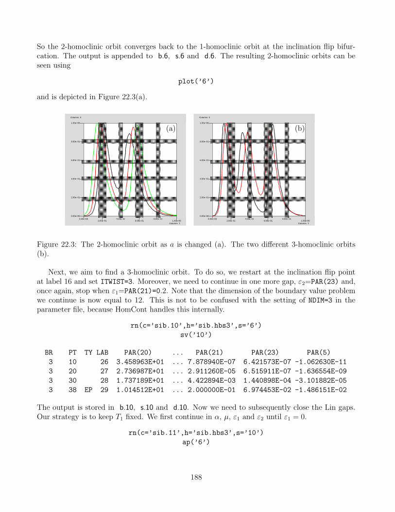
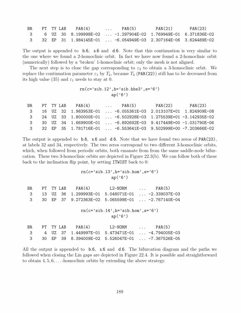
22 HomCont Demo : Homoclinic branch switching. 18322.1 Branch switching at an inclination flip in Sandstede’s model. . . . . . . . . . . . 18322.2 Branch switching for a Shil’nikov type homoclinic orbit in the FitzHugh-Nagumo
This is a guide to the software package AUTO for continuation and bifurcation problems inordinary differential equations. Earlier versions of AUTO were described in Doedel (1981), Doedel& Kernevez (1986a), Doedel & Wang (1995), Wang & Doedel (1995). For a description of thebasic algorithms see Doedel, Keller & Kernevez (1991a), Doedel, Keller & Kernevez (1991b).This version of AUTO incorporates the HomCont algorithms of Champneys & Kuznetsov (1994),Champneys, Kuznetsov & Sandstede (1996) for the bifurcation analysis of homoclinic orbits.The graphical user interface was written by Wang (1994). The Floquet multiplier algorithmswere written by Fairgrieve (1994), Fairgrieve & Jepson (1991).
Acknowledgments
The first author is much indebted to H. B. Keller of the California Institute of Technology forhis inspiration, encouragement and support. He is also thankful to AUTO users and researchcollaborators who have directly or indirectly contributed to its development, in particular, JeanPierre Kernevez, UTC, Compiegne, France; Don Aronson, University of Minnesota, Minneapolis;and Hans Othmer, University of Utah. Material in this document related to the computationof connecting orbits was developed with Mark Friedman, University of Alabama, Huntsville.Also acknowledged is the work of Nguyen Thanh Long, Concordia University, Montreal, on thegraphics program PLAUT and the pendula animation program. An earlier graphical user interfacefor AUTO on SGI machines was written by Taylor & Kevrekidis (1989). Special thanks are dueto Sheila Shull, California Institute of Technology, for her cheerful assistance in the distribution ofAUTO over a long period of time. Over the years, the development of AUTO has been supportedby various agencies through the California Institute of Technology. Work on this updated versionwas supported by a general research grant from NSERC (Canada).
The development of HomCont has much benefitted from various pieces of help and advicefrom, among others, W.-J. Beyn, Universitat Bielefeld, M. J. Friedman, University of Alabama, A.Rucklidge, University of Cambridge, M. Koper, University of Utrecht and C. J. Budd, Universityof Bristol. Financial support for collaboration was received from the U.K. Engineering andPhysical Science Research Council and the Nuffield Foundation.
8
Chapter 1
Installing AUTO .
1.1 Typographical Conventions
This manual uses the following conventions.command This font is used for commands which you can type in.PAR This font is used for AUTO parameters.filename This font is used for file and directory names.variable This font is used for environment variable.site This font is used for world wide web and ftp sites.function This font is used for function names.
1.2 Installation.
The AUTO files are available via HTTP fromhttp://www.ama.caltech.edu/∼redrod/auto2000/distribution/.
bzipped Postscript manual auto2000-0.9.6.ps.bz2gzipped Postscript manual auto2000-0.9.6.ps.gzcompressed Postscript manual auto2000-0.9.6.ps.Ztarred and gzipped source code auto2000-0.9.6.tgztarred and bzipped source code auto2000-0.9.6.tbz2tarred and compressed source code auto2000-0.9.6.tar.Zzipped source code auto2000-0.9.6.zip
Below it is assumed that you are using the Unix shell csh and that the file auto2000-0.9.6.tar.Zis in your main directory.
While in your main directory, enter the commands uncompress auto2000-0.9.6.tar.Z,followed by tar xvfo auto2000-0.9.6.tar. This will result in a directory auto, with onesubdirectory, auto/2000. Type cd auto/2000 to change directory to auto/2000. Then typeconfigure , to check your system for required compilers and libraries. Once the configurescript has finished you may then type make to compile AUTO and its ancillary software. Theconfigure script is designed to detect the details of your system which AUTO requires to compilesuccessfully. If either the configure script or the make command should fail, you may assist the
9
configure script by giving it various command line options. Please type configure --help formore details. Upon compilation, you may type make clean to remove unnecessary files.
There is a new CLUI under development which includes some of the capabilities of the oldGUI and will eventually be the recommend way to run AUTO. More information on the CLUImay be found in Chapter 4. The new CLUI does not require any additional options to be passedto the configure script.
To run the new Command Line User Interface (CLUI) and the old command language youneed to set your environment variables correctly. Assuming AUTO is installed in your homedirectory, the following commands set your environment variables so that you will be able to runthe AUTO commands, and may be placed into your .login, .profile, or .cshrc file, as appropri-ate. If you are using a sh compatible shell, such as sh, bash, ksh, or ash enter the commandsource $HOME/auto/2000/cmds/auto.env.sh. On the other hand, if you are using a csh com-patible shell, such as csh or tcsh, enter the command source $HOME/auto/2000/cmds/auto.env.csh.
There is an old and unsupported Graphical User Interface (GUI) which requires the X-Windowsystem and Motif, and it is not compiled by default. Note that AUTO can be very effectively runin Command Mode, i.e., the GUI is not strictly necessary. To compile AUTO with the old GUI,type configure --enable-gui and then make in directory auto/2000.
The PostScript conversion command @ps will be enabled if the configure script detects theappropriate software, but you may have to enter the correct printer name in auto/2000/cmds/@pr.
To generate the on-line manual, type make in auto/2000/doc.To prepare AUTO for transfer to another machine, type make superclean in directory
auto/2000 before creating the tar-file. This will remove all executable, object, and other non-essential files, and thereby reduce the size of the package.
AUTO can be tested by typing make > TEST & in directory auto/2000/test. This willexecute a selection of demos from auto/2000/demos and write a summary of the computations inthe file TEST. The contents of TEST can then be compared to other test result files in directoryauto/2000/test. Note that minor differences are to be expected due to architecture and compilerdifferences.
Some EISPACK routines used by AUTO for computing eigenvalues and Floquet multipliersare included in the package (Smith, Boyle, Dongarra, Garbow, Ikebe, Klema & Moler (1976)).
1.3 Restrictions on Problem Size.
There are size restrictions in the file auto/2000/src/auto c.h on the following AUTO -constants :the effective number of equation parameters NPAR, and the number of stored branch pointsNBIF for algebraic problems. See Chapter 5 for the significance these constants. Their maximaare denoted by the corresponding constant followed by an X. For example, NPARX in auto c.hdenotes the maximum value of NPAR. If the maxima of NBIF is exceeded in an AUTO -run thena message will be printed. On the other hand, the maximum value of NPAR, if exceeded, maylead to unreported errors. Upon installation NPARX=36; it should never be decreased below thatvalue; see also Section 6.1. Size restrictions can be changed by editing auto c.h. This must befollowed by recompilation by typing make in directory auto/2000/src.
Note that in certain cases the effective dimension may be greater than the user dimension. Forexample, for the continuation of folds, the effective dimension is 2 NDIM+1 for algebraic equations,
10
and 2 NDIM for ordinary differential equations, respectively. Similarly, for the continuation of Hopfbifurcations, the effective dimension is 3 NDIM+2.
1.4 Compatibility with Older Versions.
There are two changes compared to early versions of AUTO 94 : The user-supplied equations-files must contain the subroutine pvls. For an example of use of pvls see the demo pvl inSection 14.1. There is also a small change in the q.xxx data-file. If necessary, older AUTO 94 filescan be converted using the @94to97 command; see Section A. Data files from AUTO 97 are fullycompatible with AUTO 2000 , but as AUTO 2000 is written in C user defined function files fromAUTO 97 , which are generally in Fortran, must be rewritten.
1.5 Parallel Version.
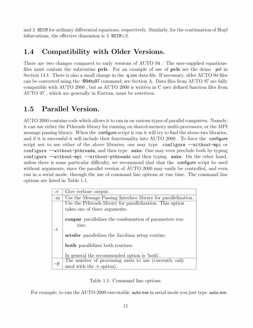
AUTO 2000 contains code which allows it to run in on various types of parallel computers. Namely,it can use either the Pthreads library for running on shared-memory multi-processors, or the MPImessage passing library. When the configure script is run it will try to find the above two libraries,and if it is successful it will include their functionality into AUTO 2000 . To force the configurescript not to use either of the above libraries, one may type configure --without-mpi orconfigure --without-pthreads, and then type make. One may even preclude both by typingconfigure --without-mpi --without-pthreads and then typing make. On the other hand,unless there is some particular difficulty, we recommend that that the configure script be usedwithout arguments, since the parallel version of AUTO 2000 may easily be controlled, and evenrun in a serial mode, through the use of command line options at run time. The command lineoptions are listed in Table 1.1.
-v Give verbose output.-m Use the Message Passing Interface library for parallelization.
-t
Use the Pthreads library for parallelization. This optiontakes one of three arguments.
conpar parallelizes the condensation of parameters rou-tine.
setubv parallelizes the Jacobian setup routine.
both parallelizes both routines.
In general the recommended option is ’both’.
-#The number of processing units to use (currently onlyused with the -t option).
Table 1.1: Command line options.
For example, to run the AUTO 2000 executable auto.exe in serial mode you just type auto.exe.
11
To run the same command in parallel using the Pthreads library on 4 processors you type auto.exe-t both -# 4. If you were to try and run the above command on a machine which did not havethe Pthreads library, the command would exit with an error and inform you that the Pthreadslibrary is not available.
Running the MPI version is somewhat more complex because of the fact that MPI normallyuses some external program for starting the computational processes. The exact name and com-mand line options of this external program depends on your MPI installation. A common namefor this MPI external program is mpirun, and a common command line option which defines thenumber of computational processes is -np. Accordingly, if you wanted to run the MPI versionof AUTO 2000 on four processors, with the above external program, you would type mpirun -np4 auto.exe -m. Please see your local MPI documentation for more detail. As with the Pthreadslibrary, if you were to try and run the above command on a machine which did not have MPI,the command would exit with an error and inform you that MPI is not available.
The commands in the auto/2000/cmds directory and described in Chapter 3 may be used withthe parallel version as well, by setting the AUTO COMMAND PREFIX and AUTO COMMAND ARGSenvironment variables. For example, to the run AUTO 2000 in parallel using the Pthreads li-brary on 4 processors just type setenv AUTO COMMAND ARGS ‘‘-t both -# 4’’ and then usethe commands in auto/2000/cmds normally. To run AUTO 97 in parallel using the MPI library on4 processors just type setenv AUTO COMMAND ARGS ‘‘-m’’ and setenv AUTO COMMAND PREFIX
‘‘mpirun -np 4’’, and then use the commands in auto/2000/cmds normally. The previous ex-amples assumed you are using the csh shell or the tcsh shell, for other shells you should modifythe commands appropriately.
12
Chapter 2
Overview of Capabilities.
2.1 Summary.
AUTO can do a limited bifurcation analysis of algebraic systems
f(u, p) = 0, f(·, ·), u ∈ Rn, (2.1)
and of systems of ordinary differential equation (ODEs) of the form
u′(t) = f(
u(t), p)
, f(·, ·), u(·) ∈ Rn, (2.2)
Here p denotes one or more free parameters.It can also do certain stationary solution and wave calculations for the partial differential
where D denotes a diagonal matrix of diffusion constants. The basic algorithms used in thepackage, as well as related algorithms, can be found in Keller (1977), Keller (1986), Doedel,Keller & Kernevez (1991a), Doedel, Keller & Kernevez (1991b).
Below, the basic capabilities of AUTO are specified in more detail. Some representative demosare also indicated.
2.2 Algebraic Systems.
Specifically, for (2.1) the program can :
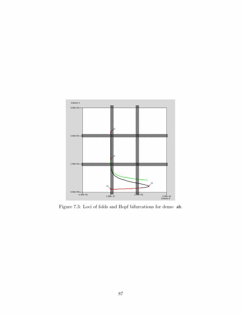
- Compute solution branches.(Demo ab; Run 1.)
- Locate branch points and automatically compute bifurcating branches.(Demo pp2; Run 1.)
- Locate Hopf bifurcation points and continue these in two parameters.(Demo ab; Runs 1 and 5.)
13
- Locate folds (limit points) and continue these in two parameters.(Demo ab; Runs 1,3,4.)
- Do each of the above for fixed points of the discrete dynamical system u(k+1) = f(u(k), p)(Demo dd2.)
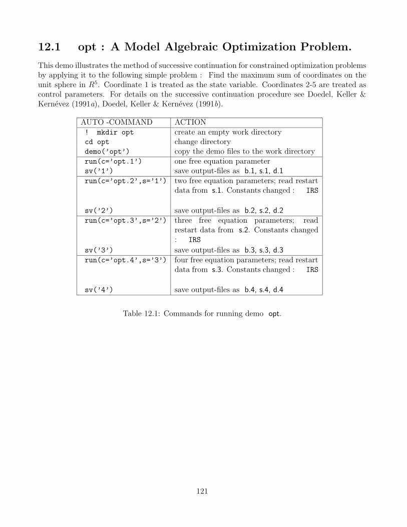
- Find extrema of an objective function along solution branches and successively continuesuch extrema in more parameters.(Demo opt.)
2.3 Ordinary Differential Equations.
For the ODE (2.2) the program can :
- Compute branches of stable and unstable periodic solutions and compute the Floquet mul-tipliers, that determine stability, along these branches. Starting data for the computationof periodic orbits are generated automatically at Hopf bifurcation points.(Demo ab; Run 2.)
- Locate folds, branch points, period doubling bifurcations, and bifurcations to tori, alongbranches of periodic solutions. Branch switching is possible at branch points and at perioddoubling bifurcations.(Demos tor, lor.)
- Continue folds and period-doubling bifurcations, in two parameters.(Demos plp, pp3.) The continuation of orbits of fixed period is also possible. This is thesimplest way to compute curves of homoclinic orbits, if the period is sufficiently large.(Demo pp2.)
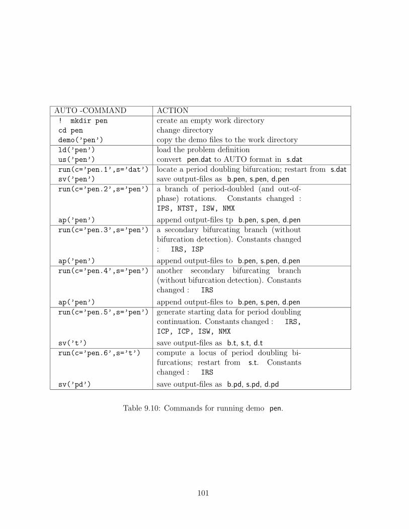
- Do each of the above for rotations, i.e., when some of the solution components are periodicmodulo a phase gain of a multiple of 2π.(Demo pen.)
- Follow curves of homoclinic orbits and detect and continue various codimension-2 bifur-cations, using the HomCont algorithms of Champneys & Kuznetsov (1994), Champneys,Kuznetsov & Sandstede (1996).(Demos san, mnt, kpr, cir, she, rev.)
- Locate extrema of an integral objective functional along a branch of periodic solutions andsuccessively continue such extrema in more parameters.(Demo ops.)
- Compute curves of solutions to (2.2) on [0, 1], subject to general nonlinear boundary andintegral conditions. The boundary conditions need not be separated, i.e., they may involveboth u(0) and u(1) simultaneously. The side conditions may also depend on parameters.The number of boundary conditions plus the number of integral conditions need not equalthe dimension of the ODE, provided there is a corresponding number of additional parameter
14
variables.(Demos exp, int.)
- Determine folds and branch points along solution branches to the above boundary valueproblem. Branch switching is possible at branch points. Curves of folds can be computedin two parameters.(Demos bvp, int.)
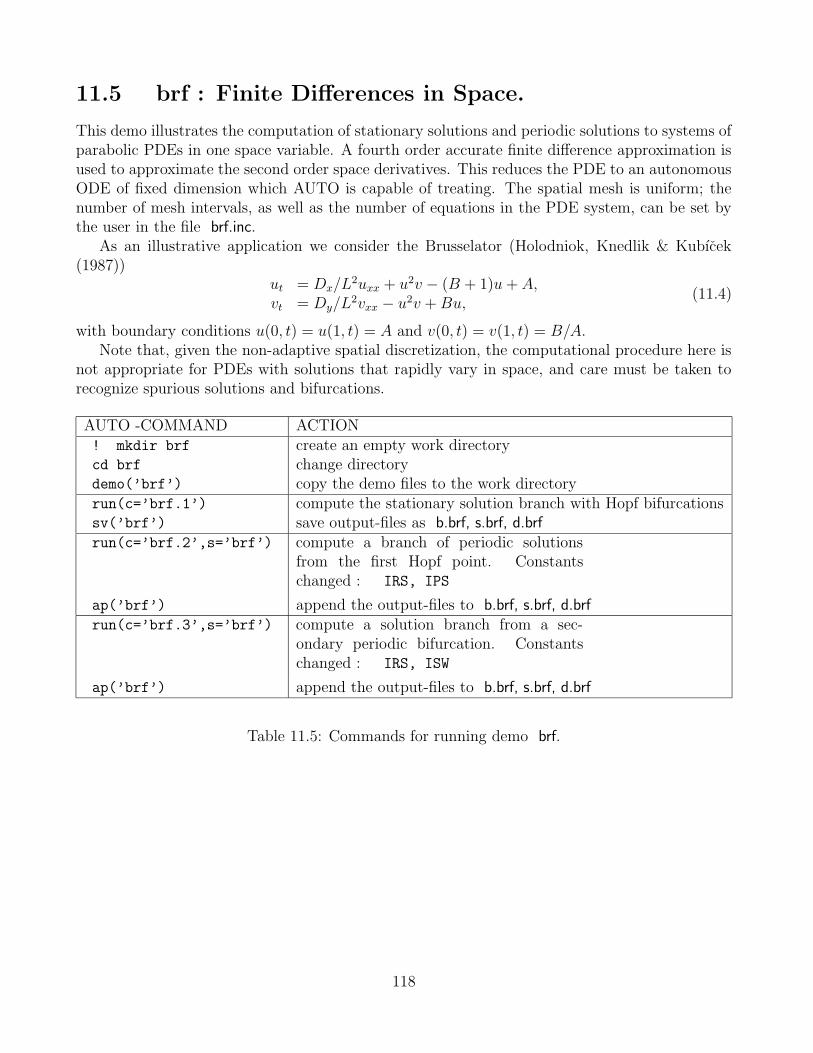
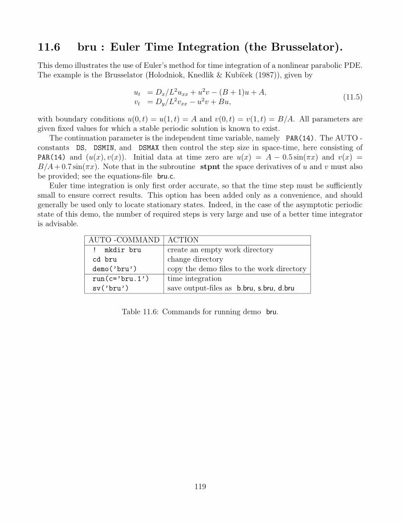
2.4 Parabolic PDEs.
For (2.3) the program can :
- Trace out branches of spatially homogeneous solutions. This amounts to a bifurcationanalysis of the algebraic system (2.1). However, AUTO uses a related system instead, inorder to enable the detection of bifurcations to wave train solutions of given wave speed.More precisely, bifurcations to wave trains are detected as Hopf bifurcations along fixedpoint branches of the related ODE
u′(z) = v(z),v′(z) = −D−1
[
c v(z) + f(
u(z), p)]
,(2.4)
where z = x− ct , with the wave speed c specified by the user.(Demo wav; Run 2.)
- Trace out branches of periodic wave solutions to (2.3) that emanate from a Hopf bifurcationpoint of Equation 2.4. The wave speed c is fixed along such a branch, but the wave lengthL, i.e., the period of periodic solutions to (2.4), will normally vary. If the wave length Lbecomes large, i.e., if a homoclinic orbit of Equation 2.4 is approached, then the wave tendsto a solitary wave solution of (2.3).(Demo wav; Run 3.)
- Trace out branches of waves of fixed wave length L in two parameters. The wave speed cmay be chosen as one of these parameters. If L is large then such a continuation gives abranch of approximate solitary wave solutions to (2.3).(Demo wav; Run 4.)
- Do time evolution calculations for (2.3), given periodic initial data on the interval [0, L].The initial data must be specified on [0, 1] and L must be set separately because of internalscaling. The initial data may be given analytically or obtained from a previous computationof wave trains, solitary waves, or from a previous evolution calculation. Conversely, if anevolution calculation results in a stationary wave then this wave can be used as startingdata for a wave continuation calculation.(Demo wav; Run 5.)
- Do time evolution calculations for (2.3) subject to user-specified boundary conditions. Asabove, the initial data must be specified on [0, 1] and the space interval length L must bespecified separately. Time evolution computations of (2.3) are adaptive in space and in time.
15
Discretization in time is not very accurate : only implicit Euler. Indeed, time integrationof (2.3) has only been included as a convenience and it is not very efficient. (Demos pd1,pd2.)
- Compute curves of stationary solutions to (2.3) subject to user-specified boundary con-ditions. The initial data may be given analytically, obtained from a previous stationarysolution computation, or from a time evolution calculation.(Demos pd1, pd2.)
In connection with periodic waves, note that (2.4) is just a special case of (2.2) and that itsfixed point analysis is a special case of (2.1). One advantage of the built-in capacity of AUTO todeal with problem (2.3) is that the user need only specify f , D, and c. Another advantage is thecompatibility of output data for restart purposes. This allows switching back and forth betweenevolution calculations and wave computations.
2.5 Discretization.
AUTO discretizes ODE boundary value problems (which includes periodic solutions) by themethod of orthogonal collocation using piecewise polynomials with 2-7 collocation points permesh interval (de Boor & Swartz (1973)). The mesh automatically adapts to the solution toequidistribute the local discretization error (Russell & Christiansen (1978)). The number of meshintervals and the number of collocation points remain constant during any given run, althoughthey may be changed at restart points. The implementation is AUTO -specific. In particular, thechoice of local polynomial basis and the algorithm for solving the linearized collocation systemswere specifically designed for use in numerical bifurcation analysis.
16
Chapter 3
How to Run AUTO .
3.1 User-Supplied Files.
The user must prepare the two files described below. This can be done with the GUI describedin Chapter 4, or independently.
3.1.1 The equations-file xxx.c
A source file xxx.c containing the C subroutines func, stpnt, bcnd, icnd, fopt, and pvls.Here xxx stands for a user-selected name. If any of these subroutines is irrelevant to the problemthen its body need not be completed. Examples are in auto/2000/demos, where, e.g., the fileab/ab.c defines a two-dimensional dynamical system, and the file exp/exp.c defines a boundaryvalue problem. The simplest way to create a new equations-file is to copy an appropriate demofile. In GUI mode, this file can be directly loaded with the GUI-button Equations/New; seeSection C.2.
3.1.2 The constants-file c.xxx
AUTO -constants for xxx.c are normally expected in a corresponding file c.xxx. Specific examplesinclude ab/c.ab and exp/c.exp in auto/2000/demos. See Chapter 5 for the significance of eachconstant.
17
3.2 User-Supplied Subroutines.
The purpose of each of the user-supplied subroutines in the file xxx.c is described below.
- func : defines the function f(u, p) in (2.1), (2.2), or (2.3).
- stpnt : This subroutine is called only if IRS=0 (see Section 5.8.5 for IRS), which typicallyis the case for the first run. It defines a starting solution (u, p) of (2.1) or (2.2). The startingsolution should not be a branch point.(Demos ab, exp, frc, lor.)
- bcnd : A subroutine bcnd that defines the boundary conditions.(Demo exp, kar.)
- icnd : A subroutine icnd that defines the integral conditions.(Demos int, lin.)
- fopt : A subroutine fopt that defines the objective functional.(Demos opt, ops.)
- pvls : A subroutine pvls for defining “solution measures”.(Demo pvl.)
3.3 Arguments of stpnt.
Note that the arguments of stpnt depend on the solution type :
- When starting from a fixed point or an analytically or numerically known space-dependentsolution, stpnt must have four arguments, namely, (NDIM,U,PAR,T). Here T is the inde-pendent space variable which takes values in the interval [0, 1]. T is ignored in the case offixed points.(Demos exp and ab.)
- Similarly, when starting from an analytically known time-periodic solution or rotation, thearguments of stpnt are (NDIM,U,PAR,T), where T denotes the independent time variablewhich takes values in the interval [0, 1]. In this case one must also specify the period inPAR(11).(Demos frc, lor, pen.)
- When using the @fc command (Section A) for conversion of numerical data, stpnt musthave four arguments, namely, (NDIM,U,PAR,T). In this case only the parameter values needto be defined in stpnt. (Demos lor and pen.)
18
3.4 User-Supplied Derivatives.
If AUTO -constant JAC equals 0 then derivatives need not be specified in func, bcnd, icnd,and fopt; see Section 5.2.4. If JAC=1 then derivatives must be given. This may be necessary forsensitive problems, and is recommended for computations in which AUTO generates an extendedsystem. Examples of user-supplied derivatives can be found in demos dd2, int, plp, opt, andops.
3.5 Output Files.
AUTO writes four output-files :
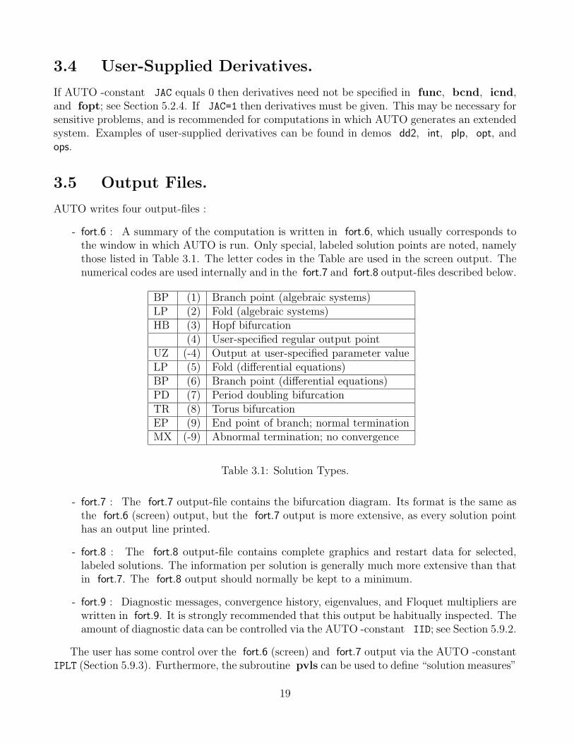
- fort.6 : A summary of the computation is written in fort.6, which usually corresponds tothe window in which AUTO is run. Only special, labeled solution points are noted, namelythose listed in Table 3.1. The letter codes in the Table are used in the screen output. Thenumerical codes are used internally and in the fort.7 and fort.8 output-files described below.
BP (1) Branch point (algebraic systems)LP (2) Fold (algebraic systems)HB (3) Hopf bifurcation
(4) User-specified regular output pointUZ (-4) Output at user-specified parameter valueLP (5) Fold (differential equations)BP (6) Branch point (differential equations)PD (7) Period doubling bifurcationTR (8) Torus bifurcationEP (9) End point of branch; normal terminationMX (-9) Abnormal termination; no convergence
Table 3.1: Solution Types.
- fort.7 : The fort.7 output-file contains the bifurcation diagram. Its format is the same asthe fort.6 (screen) output, but the fort.7 output is more extensive, as every solution pointhas an output line printed.
- fort.8 : The fort.8 output-file contains complete graphics and restart data for selected,labeled solutions. The information per solution is generally much more extensive than thatin fort.7. The fort.8 output should normally be kept to a minimum.
- fort.9 : Diagnostic messages, convergence history, eigenvalues, and Floquet multipliers arewritten in fort.9. It is strongly recommended that this output be habitually inspected. Theamount of diagnostic data can be controlled via the AUTO -constant IID; see Section 5.9.2.
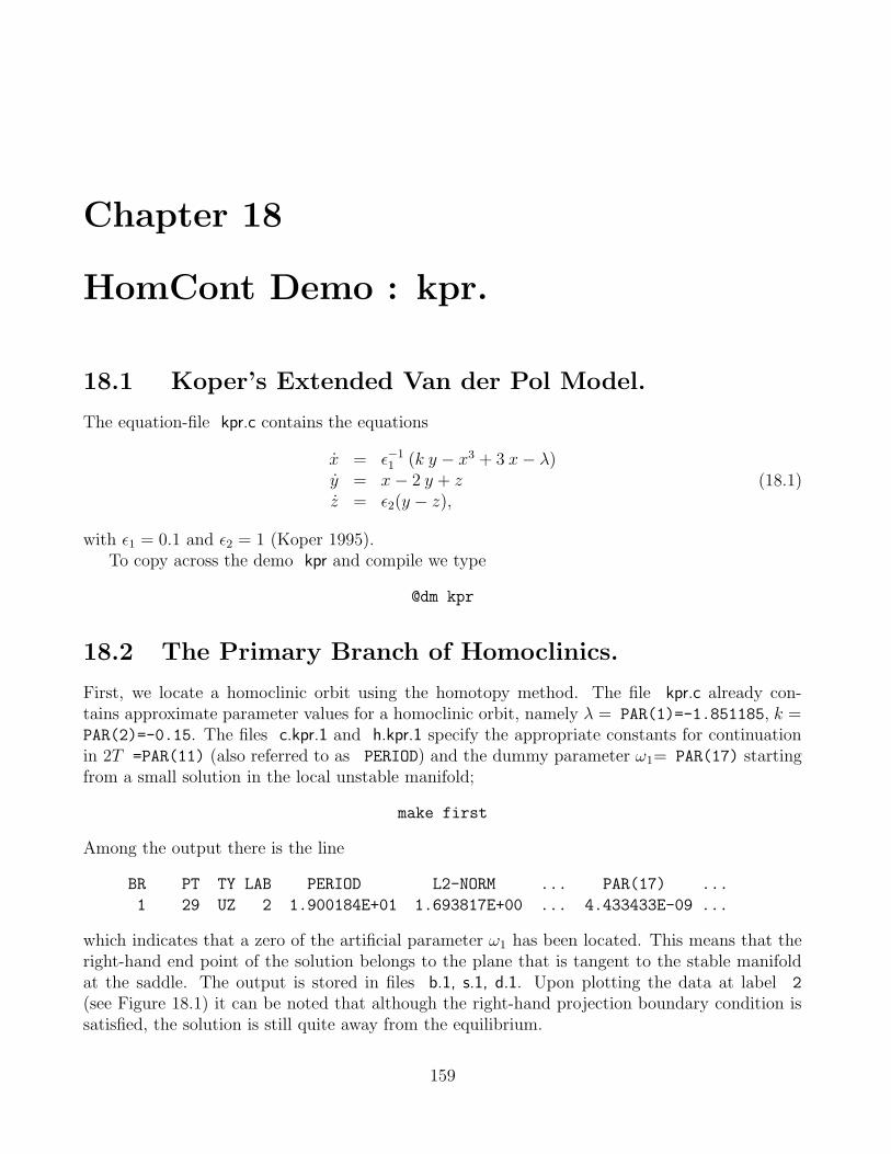
The user has some control over the fort.6 (screen) and fort.7 output via the AUTO -constantIPLT (Section 5.9.3). Furthermore, the subroutine pvls can be used to define “solution measures”
19
which can then be printed by “parameter overspecification”; see Section 5.7.10. For an examplesee demo pvl.
The AUTO -commands @sv, @ap, and @df can be used to manipulate the output-filesfort.7, fort.8, and fort.9. Furthermore, the AUTO -command @lb can be used to delete andrelabel solutions simultaneously in fort.7 and fort.8. For details see Section A.
The graphics program PLAUT can be used to graphically inspect the data in fort.7 and fort.8;see Chapter B.
20
Chapter 4
Command Line User Interface.
4.1 Typographical Conventions
This chapter uses the following conventions. All code examples will be in in the following font.
AUTO> copydemo("ab")
Copying demo ab ... done
To distinguish commands which are typed to the Unix shell from those which are typed tothe AUTO 2000 command line user interface (CLUI) we will use the following two prompts.
> Commands which follow this prompt are for the Unix shell.AUTO> Commands which follow this prompt are for the AUTO 2000 CLUI.
4.2 General Overview.
The AUTO 2000 command line user interface (CLUI) is similar to the command language de-scribed in Section A in that it facilitates the interactive creating and editing of equations-filesand constants-files. It differs from the other command language in that it is based on the object-oriented scripting language Python (see Lutz (1996)) and provides extensive programming ca-pabilities. This chapter will provide documentation for the AUTO 2000 CLUI commands, butis not intended as a tutorial for the Python language. We will attempt to make this chapterself contained by describing all Python constructs that we use in the examples, but for moreextensive documentation on the Python language, including tutorials and pointers to furtherdocumentation, please see Lutz (1996) or the web page http://www.python.org which containsan excellent tutorial at http://www.python.org/doc/current/tut/tut.html.
To use the CLUI for a new equation, change to an empty directory. For an existing equations-file, change to its directory. (Do not activate the CLUI in the directory auto/2000 or in any ofits subdirectories.) Then type
auto.If your command search path has been correctly set (see Section 1.2), this command will
start the AUTO 2000 CLUI interactive interpretor and provide you with the AUTO 2000 CLUIprompt.
21
> auto
Initializing
Python 1.5.2 (1, Feb 1 2000, 16:32:16) [GCC egcs-2.91.66 19990314/Linux
Figure 4.1: Typing auto at the Unix shell prompt starts the AUTO 2000 CLUI.
In addition to the examples in the following sections there are several example scripts whichcan be found in auto/2000/demos/python and are listed in Table 4.1. These scripts are fullyannotated and provide good examples of how AUTO 2000 CLUI scripts are written. The scriptsin auto/2000/demos/python/n-body are espcially lucid examples and preform various related partsof a calculation involving the gravitional N-body problem. Scripts which end in the suffix .autoare called “basic” scripts and can be run by typing auto scriptname.auto. The scripts show inSection 4.3 and Section 4.5 are examples of basic scripts. Scripts which end in the suffix .xauto arecalled “expert” scripts and can be run by typing autox scriptname.xauto. More informationon expert scripts can be found in Section 4.6. See the README file in that directory for moreinformation.
4.3 First Example
We begin with a simple example of the AUTO 2000 CLUI. In this example we copy the ab demofrom the AUTO 2000 installation directory and run it. For more information on the ab demo seeSection 7.2. The commands listed in Table 4.2 will copy the demo files to your work directory andrun the first part of the demo. The results of running these commands are shown in Figure 4.2.
Let us examine more closely what action each of the commands performs. First, copydemo(’ab’)(Section 4.13.7 in the reference) copies the files in $AUTO DIR/demo/ab into the work directory.
Next, load(equation=’ab’) (Section 4.13.33 in the reference) informs the AUTO 2000 CLUIthat the name of the user defined function file is ab.c. The command load is one of the mostcommonly used commands in the AUTO 2000 CLUI, since it reads and parses the user files whichare manipulated by other commands. The AUTO 2000 CLUI stores this setting until it is changedby a command, such as another load command. The idea of storing information is one of theideas that sets the CLUI apart from the command language described in Section A.
Next, load(constants=’ab.1’) parses the AUTO constants file c.ab.1 and reads it intomemory. Note that changes to the file c.ab.1 after it has been loaded in will not be used byAUTO 2000 unless it is loaded in again after the changes are made.
Finally, run() (Section 4.13.31 in the reference) uses the user defined functions loaded by theload(equation=’ab’) command, and the AUTO constants loaded by the load(constants=’ab.1’)to run AUTO 2000 .
Figure 4.2 showed two of the file types that the load command can read into memory, namelythe user defined function file and the AUTO constants file (Section 3.1). There are two otherfiles types that can be read in using the load command, and they are the restart solution file(Section 3.5) and the HomCont parameter file (Section 15.2).
22
Script Description
demo1.auto The demo script from Section 4.3.
demo2.auto The demo script from Section 4.5.
userScript.xauto The expert demo script from Figure 4.11.
userScript.pyThe loadable expert demo script from Fig-ure 4.12.
fullTest.autoA script which uses the entireAUTO 2000 command set, except forthe plotting commands.
plotter.autoA demonstration of some of the plottingcapabilities of AUTO 2000 .
fullTest.autoA script which implements the tutorialfrom Section 7.2.
n-body/compute lagrange points family.autoA basic script which computes and plots allof the “Lagrange points” as a function ofthe ratio of the masses of the two planets.
n-body/compute lagrange points 0.5.auto
A basic script which computes all of the“Lagrange points” for the case where themasses of the two planets are equal, andsaves the data.
n-body/compute periodic family.xauto
An expert script which starts at a“Lagrange point” computed by com-pute lagrange points 0.5.auto and contin-ues in the ratio of the masses until a spec-ified mass ratio is reached. It then com-putes a family of periodic orbits for eachpair of purely complex eigenvalues.
n-body/to matlab.xauto
A script which takes a set ofAUTO 2000 data files and creates aset of files formatted for importing intoMatlab for either plotting or furthercalculations.
Table 4.1: The various demonstration scripts for the AUTO 2000 CLUI.
23
Unix-COMMAND ACTIONauto start the AUTO 2000 CLUI
AUTO 2000 CLUI COMMAND ACTIONcopydemo(’ab’) copy the demo files to the work directoryload(equation=’ab’) load the filename ab.c into memoryload(constants=’ab.1’) load the contents of the file r.ab.1 into memoryrun() run AUTO 2000 with the current set of files
Table 4.2: Running the demo ab files.
> auto
Initializing
Python 1.5.2 (#1, Feb 1 2000, 16:32:16) [GCC egcs-2.91.66 19990314/Linux
1 92 EP 5 1.512417E-01 4.369748E+00 9.155894E-01 4.272750E+00
Total Time 9.502E-02
ab ... done
AUTO>
Figure 4.2: Typing auto at the Unix shell prompt starts the AUTO 2000 CLUI. The rest of thecommands are interpreted by the AUTO 2000 CLUI.
24
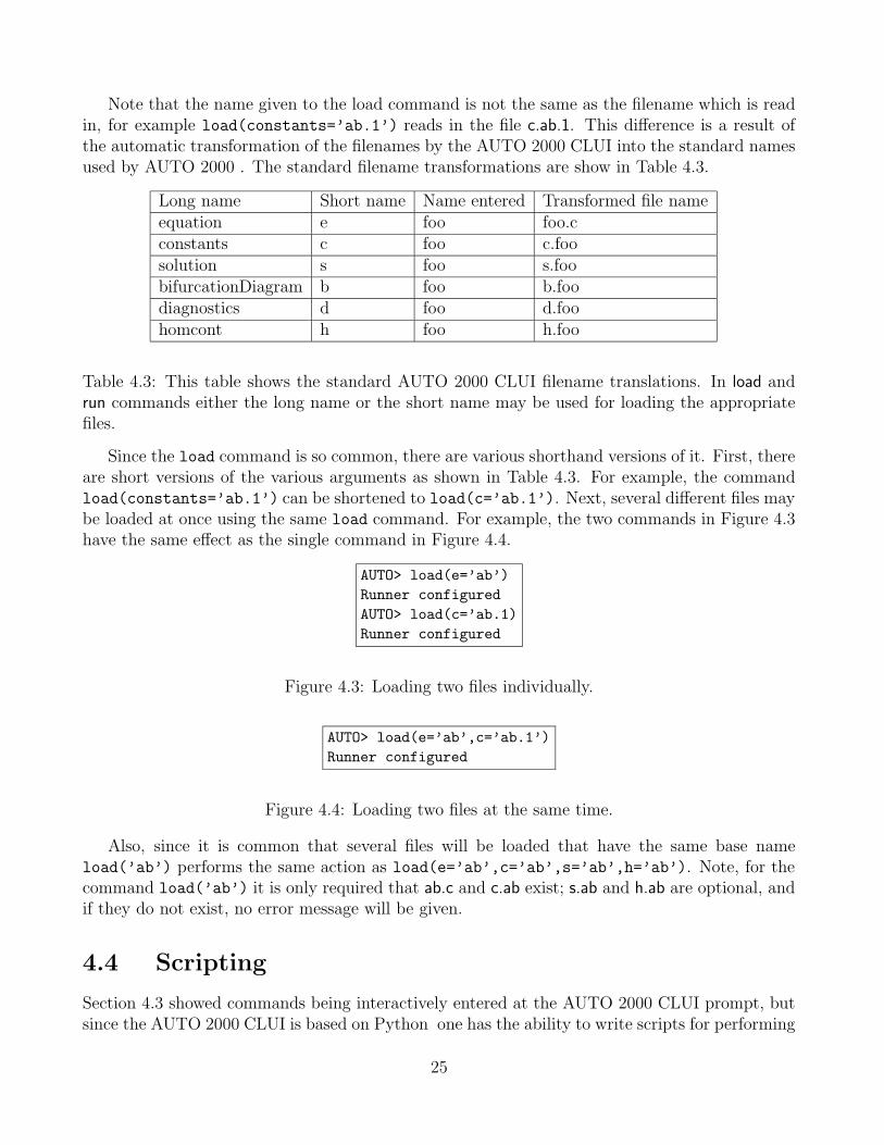
Note that the name given to the load command is not the same as the filename which is readin, for example load(constants=’ab.1’) reads in the file c.ab.1. This difference is a result ofthe automatic transformation of the filenames by the AUTO 2000 CLUI into the standard namesused by AUTO 2000 . The standard filename transformations are show in Table 4.3.
Long name Short name Name entered Transformed file nameequation e foo foo.cconstants c foo c.foosolution s foo s.foobifurcationDiagram b foo b.foodiagnostics d foo d.foohomcont h foo h.foo
Table 4.3: This table shows the standard AUTO 2000 CLUI filename translations. In load andrun commands either the long name or the short name may be used for loading the appropriatefiles.
Since the load command is so common, there are various shorthand versions of it. First, thereare short versions of the various arguments as shown in Table 4.3. For example, the commandload(constants=’ab.1’) can be shortened to load(c=’ab.1’). Next, several different files maybe loaded at once using the same load command. For example, the two commands in Figure 4.3have the same effect as the single command in Figure 4.4.
AUTO> load(e=’ab’)
Runner configured
AUTO> load(c=’ab.1)
Runner configured
Figure 4.3: Loading two files individually.
AUTO> load(e=’ab’,c=’ab.1’)
Runner configured
Figure 4.4: Loading two files at the same time.
Also, since it is common that several files will be loaded that have the same base nameload(’ab’) performs the same action as load(e=’ab’,c=’ab’,s=’ab’,h=’ab’). Note, for thecommand load(’ab’) it is only required that ab.c and c.ab exist; s.ab and h.ab are optional, andif they do not exist, no error message will be given.
4.4 Scripting
Section 4.3 showed commands being interactively entered at the AUTO 2000 CLUI prompt, butsince the AUTO 2000 CLUI is based on Python one has the ability to write scripts for performing
25
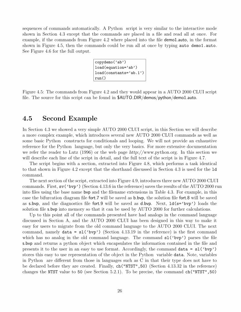
sequences of commands automatically. A Python script is very similar to the interactive modeshown in Section 4.3 except that the commands are placed in a file and read all at once. Forexample, if the commands from Figure 4.2 where placed into the file demo1.auto, in the formatshown in Figure 4.5, then the commands could be run all at once by typing auto demo1.auto.See Figure 4.6 for the full output.
copydemo(’ab’)
load(equation=’ab’)
load(constants=’ab.1’)
run()
Figure 4.5: The commands from Figure 4.2 and they would appear in a AUTO 2000 CLUI scriptfile. The source for this script can be found in $AUTO DIR/demos/python/demo1.auto.
4.5 Second Example
In Section 4.3 we showed a very simple AUTO 2000 CLUI script, in this Section we will describea more complex example, which introduces several new AUTO 2000 CLUI commands as well assome basic Python constructs for conditionals and looping. We will not provide an exhaustivereference for the Python language, but only the very basics. For more extensive documentationwe refer the reader to Lutz (1996) or the web page http://www.python.org. In this section wewill describe each line of the script in detail, and the full text of the script is in Figure 4.7.
The script begins with a section, extracted into Figure 4.8, which performs a task identicalto that shown in Figure 4.2 except that the shorthand discussed in Section 4.3 is used for the ld
command.The next section of the script, extracted into Figure 4.9, introduces three new AUTO 2000 CLUI
commands. First, sv(’bvp’) (Section 4.13.6 in the reference) saves the results of the AUTO 2000 runinto files using the base name bvp and the filename extensions in Table 4.3. For example, in thiscase the bifurcation diagram file fort.7 will be saved as b.bvp, the solution file fort.8 will be savedas s.bvp, and the diagnostics file fort.9 will be saved as d.bvp. Next, ld(s=’bvp’) loads thesolution file s.bvp into memory so that it can be used by AUTO 2000 for further calculations.
Up to this point all of the commands presented have had analogs in the command languagediscussed in Section A, and the AUTO 2000 CLUI has been designed in this way to make iteasy for users to migrate from the old command language to the AUTO 2000 CLUI. The nextcommand, namely data = sl(’bvp’) (Section 4.13.19 in the reference) is the first commandwhich has no analog in the old command language. The command sl(’bvp’) parses the files.bvp and returns a python object which encapsulates the information contained in the file andpresents it to the user in an easy to use format. Accordingly, the command data = sl(’bvp’)
stores this easy to use representation of the object in the Python variable data. Note, variablesin Python are different from those in languages such as C in that their type does not have tobe declared before they are created. Finally, ch("NTST",50) (Section 4.13.32 in the reference)changes the NTST value to 50 (see Section 5.2.1). To be precise, the command ch("NTST",50)
1 92 EP 5 1.512417E-01 4.369748E+00 9.155894E-01 4.272750E+00
Total Time 8.740E-02
ab ... done
>
Figure 4.6: This Figure starts by listing the contents of the demo1.auto file using the Unix cat
command. The file is then run through the AUTO 2000 CLUI by typing auto demo1.auto andthe output is shown.
only modifies the “in memory” version of the AUTO 2000 constants created by the ld(’bvp’)
command. The original file c.bvp is not modified.The next section of the script, extracted into Figure 4.10, shows as example of looping and
conditionals in an AUTO 2000 CLUI script. The first line for solution in data: is thePython syntax for loops. The data variable was defined in Figure 4.9 to be the parsed ver-sion of an AUTO 2000 fort.8 file, and accordingly contains a list of the solutions from the fort.8file. The command for solution in data: is used to loop over all solutions in the data variableby setting the variable solution to be one of the solutions in data and then calling the rest ofthe code in the block.
Python differs from most other computer languages in that blocks of code are not defined bysome delimiter, such as {} in C, but by indentation. In Figure 4.7 the commands plot(’bvp’)
and wait() are not part of the loop, because they are indented differently. This can be confusingfirst time users of Python , but it has the advantage that the code is forced to have a consistentindentation style.
The next command in the script, if solution["Type name"] == "BP": is a Python condi-
27
copydemo(’bvp’)
ld(’bvp’)
run()
sv(’bvp’)
ld(s=’bvp’)
data = sl(’bvp’)
ch("NTST",50)
for solution in data:
if solution["Type name"] == "BP":
ch("IRS", solution["Label"])
ch("ISW", -1)
# Compute forward
run()
ap(’bvp’)
# Compute back
ch("DS",-pr("DS"))
run()
ap(’bvp’)
plot(’bvp’)
wait()
Figure 4.7: This Figure shows a more complex AUTO 2000 CLUI script. The source for thisscript can be found in $AUTO DIR/demos/python/demo2.auto.
copydemo(’bvp’)
ld(’bvp’)
run()
Figure 4.8: The first part of the complex AUTO 2000 CLUI script.
sv(’bvp’)
ld(s=’bvp’)
data = sl(’bvp’)
ch("NTST",50)
Figure 4.9: The second part of the complex AUTO 2000 CLUI script.
28
tional. It examines the contents of the variable solution (which is one of the entries in the arrayof solutions data) and checks to see if the condition solution["Type name"] == "BP" holds.For parsed fort.8 files Type name BP corresponds to a bifurcation point. Accordingly, the functionof this loop and conditional is to examine every solution in the fort.8 file and run the followingcommands if the solution is a bifurcation point.
The next line is ch("IRS", solution["Label"]) which changes the “in memory” version ofthe AUTO 2000 constants file to set IRS (see Section 5.8.5) equal to the label of the bifurcationpoint. We then use ch("ISW", -1) to change the AUTO 2000 constant ISW to -1, which indicatesa branch switch (see Section 5.8.3).
We then use a run() command to perform the calculation of the bifurcating branch and thenappend the data to the s.bvp, b.bvp, and d.bvp files with the ap(’bvp’) command (Section 4.13.1in the reference). In addition, as can be seen in Figure 4.10, the # character is the Python com-ment character. When the Python interpretor encounters a # character it ignores everythingfrom that character to the end of the line.
Finally, we us ch("DS",-pr("DS")) to change the AUTO 2000 initial step size from positiveto negative, which allows us to compute the bifurcating branch in the other direction (see Sec-tion 5.5.1). Running the AUTO 2000 calculation with the run() command and appending thedata the appropriate files with the ap(’bvp’) command completes the body of the loop.
for solution in data:
if solution["Type name"] == "BP":
ch("IRS", solution["Label"])
ch("ISW", -1)
# Compute forward
run()
ap(’bvp’)
# Compute back
ch("DS",-pr("DS"))
run()
ap(’bvp’)
Figure 4.10: The second part of the complex AUTO 2000 CLUI script.
Now that the section of script shown in Figure 4.10 has finished computing the bifurcationdiagram, the command plot(’bvp’) brings up a plotting window (Section 4.13.20 in the ref-erence), and the command wait() causes the AUTO 2000 CLUI to wait for input. You maynow exit the AUTO 2000 CLUI by pressing any key in the window in which you started theAUTO 2000 CLUI.
4.6 Extending the AUTO 2000 CLUI
The code in Figure 4.7 performed a very useful and common procedure, it started an AUTO 2000 cal-culation and performed additional continuations at every point which AUTO 2000 detected as abifurcation. Unfortunately, the script as written can only be used for the bvp demo. In this sec-tion we will generalize the script in Figure 4.7 for use with any demo, and demonstrate how it can
29
be imported back into the interactive mode to create a new command for the AUTO 2000 CLUI.Several examples of such “expert” scripts can be found in auto/2000/demos/python/n-body.
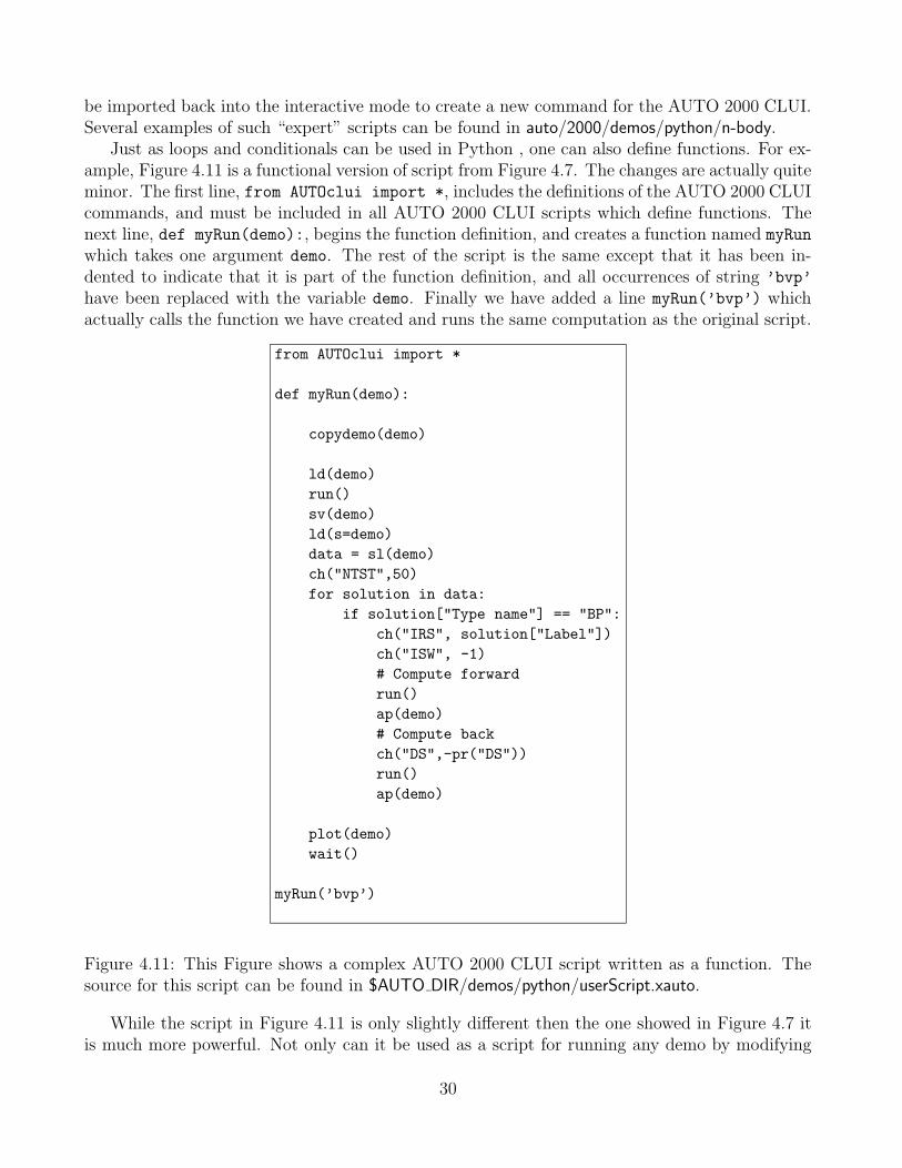
Just as loops and conditionals can be used in Python , one can also define functions. For ex-ample, Figure 4.11 is a functional version of script from Figure 4.7. The changes are actually quiteminor. The first line, from AUTOclui import *, includes the definitions of the AUTO 2000 CLUIcommands, and must be included in all AUTO 2000 CLUI scripts which define functions. Thenext line, def myRun(demo):, begins the function definition, and creates a function named myRun
which takes one argument demo. The rest of the script is the same except that it has been in-dented to indicate that it is part of the function definition, and all occurrences of string ’bvp’
have been replaced with the variable demo. Finally we have added a line myRun(’bvp’) whichactually calls the function we have created and runs the same computation as the original script.
from AUTOclui import *
def myRun(demo):
copydemo(demo)
ld(demo)
run()
sv(demo)
ld(s=demo)
data = sl(demo)
ch("NTST",50)
for solution in data:
if solution["Type name"] == "BP":
ch("IRS", solution["Label"])
ch("ISW", -1)
# Compute forward
run()
ap(demo)
# Compute back
ch("DS",-pr("DS"))
run()
ap(demo)
plot(demo)
wait()
myRun(’bvp’)
Figure 4.11: This Figure shows a complex AUTO 2000 CLUI script written as a function. Thesource for this script can be found in $AUTO DIR/demos/python/userScript.xauto.
While the script in Figure 4.11 is only slightly different then the one showed in Figure 4.7 itis much more powerful. Not only can it be used as a script for running any demo by modifying
30
the last line, it can be read back into the interactive mode of the AUTO 2000 CLUI and usedto create a new command, as in Figure 4.12. First, we create a file called userScript.py whichcontains the script from Figure 4.11, with one minor modification. We want the function onlyto run when we use it interactively, not when the file userScript.py is read in, so we remove thelast line where the function is called. We start the AUTO 2000 CLUI with the Unix commandauto, and once the AUTO 2000 CLUI is running we use the command from userScript import
*, to import the file userScript.py into the AUTO 2000 CLUI. The import command makes allfunctions in that file available for our use (in this case myRun is the only one). It is importantto note that from userScript import * does not use the .py extension on the file name. Afterimporting our new function, we may use it just like any other function in the AUTO 2000 CLUI,for example by typing myRun(’bvp’).
4.7 Bifurcation Diagram Files
Using the commandParseDiagramFile command (Section 4.13.18 in the reference) the user canparse and read into memory an AUTO 2000 bifurcation diagram file. For example, the com-mand commandParseDiagramFile(’ab’) would parse the file b.ab (if you are using the standardfilename translations from Table 4.3) and return an object which encapsulates the bifurcationdiagram in an easy to use form.
The object returned by the commandParseDiagramFile is a list of all of the solutions in theappropriate bifurcation diagram file, and each solution is a Python dictionary with entries foreach piece of data for the solution. For example, the sequence of commands in Figure 4.13, printsout the label of the first solution in a bifurcation diagram. The queriable parts of the object arelisted in Table 4.4.
The individual elements of the array may be accessed in two ways, either by index of thesolution using the [] syntax or by label number using the () syntax. For example, assumethat the parsed object is contained in a variable data. The first solution may be accessed usingthe command data[0], while the solution with label 57 may be accessed using the commanddata(57).
This class has two methods that are particularily useful for creating data which can be usedin other programs. First, there is a method called toArray which takes a bifurcation diagramand returns a standard Python array. Second, there is a method called writeRawFilename
which will create a standard ASCII file which contains the bifurcation diagram. For example,we again assume that the parsed object is contained in a variable data. If one wanted to havethe bifurcation diagram returned as a Python array one would type data.toArray(). Similar-ily, if one wanted to write out the bifurcation diagram to the file outputfile one would typedata.writeRawFilename(’outputfile’).
4.8 Solution Files
Using the commandParseSolutionFile command (Section 4.13.19 in the reference) the user canparse and read into memory an AUTO 2000 bifurcation solution file. For example, the commandcommandParseSolutionFile(’ab’) would parse the file b.ab (if you are using the standard file-
31
> cp \$AUTO\_DIR/python/demo/userScript.py .
> ls
userScript.py
> cat userScript.py
# This is an example script for the AUTO2000 command line user
# interface. See the "Command Line User Interface" chapter in the
# manual for more details.
from AUTOclui import *
def myRun(demo):
copydemo(demo)
ld(demo)
run()
sv(demo)
ld(s=demo)
data = sl(demo)
ch("NTST",50)
for solution in data:
if solution["Type name"] == "BP":
ch("IRS", solution["Label"])
ch("ISW", -1)
# Compute forward
run()
ap(demo)
# Compute back
ch("DS",-pr("DS"))
run()
ap(demo)
plot(demo)
wait()
> auto
Initializing
Python 1.5.2 (#1, Feb 1 2000, 16:32:16) [GCC egcs-2.91.66 19990314/Linux
Figure 4.12: This Figure shows the functional version of the AUTO 2000 CLUI from Figure 4.11being used as an extension to the AUTO 2000 CLUI. The source code for this script can be foundin $AUTO DIR/python/demo/userScript.py
Figure 4.13: This figure shows an example of parsing a bifurcation diagram. The first command,data=dg(’ab’), reads in the bifurcation diagram and puts it into the variable data. The secondcommand, print data[0] prints out all of the data about the first solution in the list. The thirdcommand, print data[0][’LAB’], prints out the label of the first point.
Query string MeaningTY name The short name for the solution type (see Table 4.5).TY number The number of the solution type (see Table 4.5).BR The branch number.PT The point number.LAB The solution label, if any.section A unique identifier for each branch in a file with multiple branches.data An array which contains the AUTO 2000 output.
Table 4.4: This table shows the strings that can be used to query a bifurcation diagram objectand their meanings.
Type Short Name NumberNo Label No LabelBranch point (algebraic problem) BP 1Fold (algebraic problem) LP 2Hopf bifurcation (algebraic problem) HB 3Regular point (every NPR steps) RG 4User requested point UZ -4Fold (ODE) LP 5Bifurcation point (ODE) BP 6Period doubling bifurcation (ODE) PD 7Bifurcation to invarient torus (ODE) TR 8Normal begin or end EP 9Abnormal termination MX -9
Table 4.5: This table shows the the various types of points that can be in solution and bifurcationdiagram files, with their short names and numbers.
33
name translations from Table 4.3) and return an object which encapsulates the bifurcation solutionin a easy to use form.
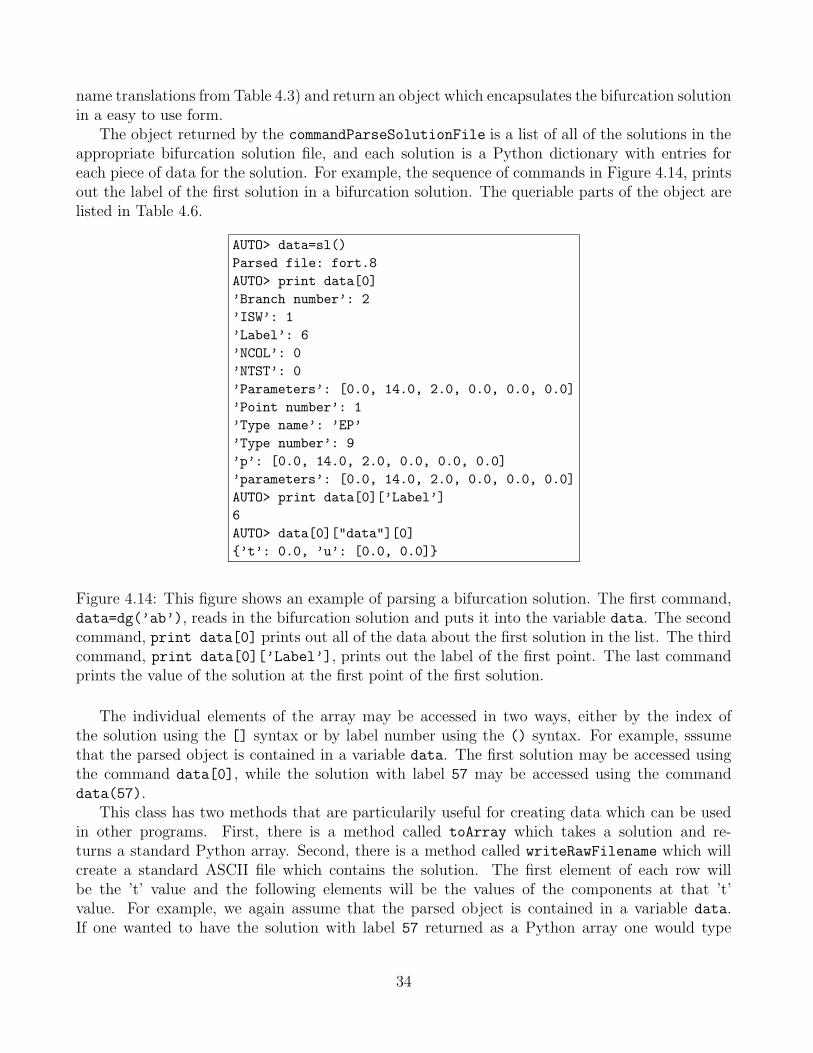
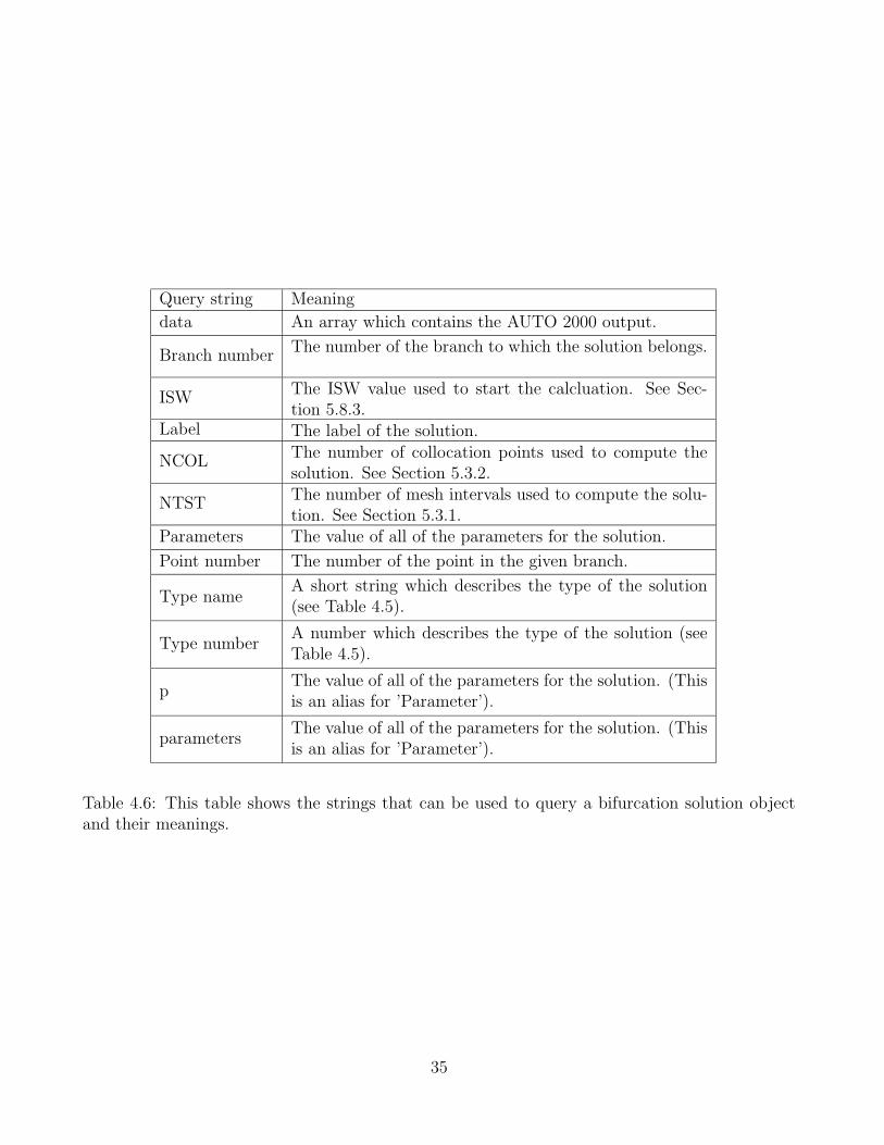
The object returned by the commandParseSolutionFile is a list of all of the solutions in theappropriate bifurcation solution file, and each solution is a Python dictionary with entries foreach piece of data for the solution. For example, the sequence of commands in Figure 4.14, printsout the label of the first solution in a bifurcation solution. The queriable parts of the object arelisted in Table 4.6.
AUTO> data=sl()
Parsed file: fort.8
AUTO> print data[0]
’Branch number’: 2
’ISW’: 1
’Label’: 6
’NCOL’: 0
’NTST’: 0
’Parameters’: [0.0, 14.0, 2.0, 0.0, 0.0, 0.0]
’Point number’: 1
’Type name’: ’EP’
’Type number’: 9
’p’: [0.0, 14.0, 2.0, 0.0, 0.0, 0.0]
’parameters’: [0.0, 14.0, 2.0, 0.0, 0.0, 0.0]
AUTO> print data[0][’Label’]
6
AUTO> data[0]["data"][0]
{’t’: 0.0, ’u’: [0.0, 0.0]}
Figure 4.14: This figure shows an example of parsing a bifurcation solution. The first command,data=dg(’ab’), reads in the bifurcation solution and puts it into the variable data. The secondcommand, print data[0] prints out all of the data about the first solution in the list. The thirdcommand, print data[0][’Label’], prints out the label of the first point. The last commandprints the value of the solution at the first point of the first solution.
The individual elements of the array may be accessed in two ways, either by the index ofthe solution using the [] syntax or by label number using the () syntax. For example, sssumethat the parsed object is contained in a variable data. The first solution may be accessed usingthe command data[0], while the solution with label 57 may be accessed using the commanddata(57).
This class has two methods that are particularily useful for creating data which can be usedin other programs. First, there is a method called toArray which takes a solution and re-turns a standard Python array. Second, there is a method called writeRawFilename which willcreate a standard ASCII file which contains the solution. The first element of each row willbe the ’t’ value and the following elements will be the values of the components at that ’t’value. For example, we again assume that the parsed object is contained in a variable data.If one wanted to have the solution with label 57 returned as a Python array one would type
34
Query string Meaning
data An array which contains the AUTO 2000 output.
Branch numberThe number of the branch to which the solution belongs.
ISWThe ISW value used to start the calcluation. See Sec-tion 5.8.3.
Label The label of the solution.
NCOLThe number of collocation points used to compute thesolution. See Section 5.3.2.
NTSTThe number of mesh intervals used to compute the solu-tion. See Section 5.3.1.
Parameters The value of all of the parameters for the solution.
Point number The number of the point in the given branch.
Type nameA short string which describes the type of the solution(see Table 4.5).
Type numberA number which describes the type of the solution (seeTable 4.5).
pThe value of all of the parameters for the solution. (Thisis an alias for ’Parameter’).
parametersThe value of all of the parameters for the solution. (Thisis an alias for ’Parameter’).
Table 4.6: This table shows the strings that can be used to query a bifurcation solution objectand their meanings.
35
data(57).toArray(). Similarily, if one wanted to write out the solution to the file outputfile
one would type data(57).writeRawFilename(’outputfile’).
4.9 The .autorc File
Much of the default behavior of the AUTO 2000 CLUI can be controlled by the .autorc file. The.autorc file can exist in either the main AUTO 2000 directory, the users home directory, or thecurrent directory. For any option which is defined in more then one file, the .autorc file in thecurrent directory (if it exists) takes precedence, followed by the .autorc file in the users homedirectory (if it exists), and then the .autorc file in the main AUTO 2000 directory. Hence, optionsmay be defined on either a per directory, per user, or global basis.
The first section of the .autorc file begins with the line [AUTO command aliases] and thissection defines short names, or aliases, for the AUTO 2000 CLUI commands. Each line thereafteris a definition of a command, similiar to branchPoint =commandQueryBranchPoint. The righthand side of the assignment is the internal AUTO 2000 CLUI name for the command, while theleft hand side is the desired alias. Aliases and internal names may be used interchangably, butthe intention is that the aliases will be more commonly used. A default set of aliases is provided,and these aliases will be used in the examples in the rest of this Chapter. The default aliases arelisted in the reference in Section 4.13.
NOTE: Defaults for the plotting tool may be included in the .autorc file as well. The docu-mentation for this is under developement, but the file $AUTO DIR/.autorc contains examples ofhow these options may be set.
4.10 Two Dimensional Plotting Tool
The two dimensional plotting tool can be run by using the command plot() to plot the filesfort.7 and fort.8 after a calculation has been run, or using the command plot(’foo’) to plotethe data in the files s.foo and b.foo.
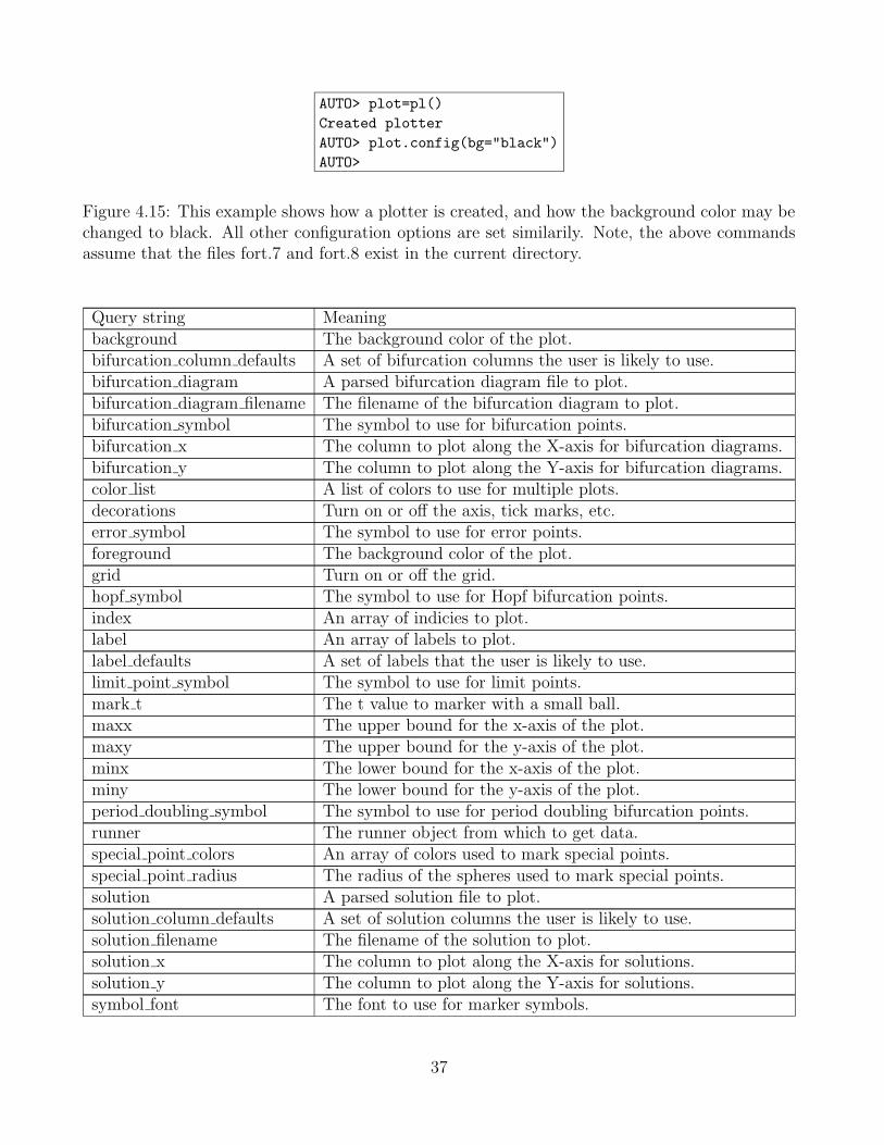
The menu bar provides two buttons. The File button brings up a menu which allows theuser to save the current plot as a Postscript file or to quit the plotter. The Options button allowsthe plotter configuration options to be modified. The available options are decribed in Table 4.7.In addition, the options can be set from within the CLUI. For example, the set of commandsin Figure 4.15 shows how to create a plotter and change its background color to black. Thedemo script auto/2000/demo/python/plotter.py contains several examples of changing options inplotters.
Pressing the right mouse button in the plotting window brings up a menu of buttons whichcontrol several aspects of the plotting window. The top two toggle buttons control what func-tion the left button performs. The print value button causes the left button to print out thenumerical value underneath the pointer when it is clicked. When zoom button is checked the leftmouse button may be held down to create a box in the plot. When the left button is released theplot will zoom to the selected portion of the diagram. The unzoom button returns the diagramto the default zoom. The Postscript button allows the user to save the plot as a Postscript file.The Configure... button brings up the dialog for setting configuration options.
36
AUTO> plot=pl()
Created plotter
AUTO> plot.config(bg="black")
AUTO>
Figure 4.15: This example shows how a plotter is created, and how the background color may bechanged to black. All other configuration options are set similarily. Note, the above commandsassume that the files fort.7 and fort.8 exist in the current directory.
Query string Meaningbackground The background color of the plot.bifurcation column defaults A set of bifurcation columns the user is likely to use.bifurcation diagram A parsed bifurcation diagram file to plot.bifurcation diagram filename The filename of the bifurcation diagram to plot.bifurcation symbol The symbol to use for bifurcation points.bifurcation x The column to plot along the X-axis for bifurcation diagrams.bifurcation y The column to plot along the Y-axis for bifurcation diagrams.color list A list of colors to use for multiple plots.decorations Turn on or off the axis, tick marks, etc.error symbol The symbol to use for error points.foreground The background color of the plot.grid Turn on or off the grid.hopf symbol The symbol to use for Hopf bifurcation points.index An array of indicies to plot.label An array of labels to plot.label defaults A set of labels that the user is likely to use.limit point symbol The symbol to use for limit points.mark t The t value to marker with a small ball.maxx The upper bound for the x-axis of the plot.maxy The upper bound for the y-axis of the plot.minx The lower bound for the x-axis of the plot.miny The lower bound for the y-axis of the plot.period doubling symbol The symbol to use for period doubling bifurcation points.runner The runner object from which to get data.special point colors An array of colors used to mark special points.special point radius The radius of the spheres used to mark special points.solution A parsed solution file to plot.solution column defaults A set of solution columns the user is likely to use.solution filename The filename of the solution to plot.solution x The column to plot along the X-axis for solutions.solution y The column to plot along the Y-axis for solutions.symbol font The font to use for marker symbols.
37
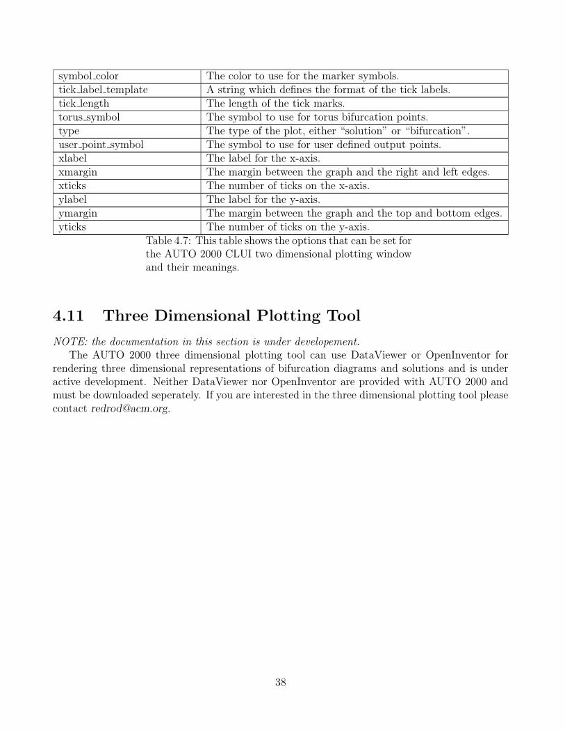
symbol color The color to use for the marker symbols.tick label template A string which defines the format of the tick labels.tick length The length of the tick marks.torus symbol The symbol to use for torus bifurcation points.type The type of the plot, either “solution” or “bifurcation”.user point symbol The symbol to use for user defined output points.xlabel The label for the x-axis.xmargin The margin between the graph and the right and left edges.xticks The number of ticks on the x-axis.ylabel The label for the y-axis.ymargin The margin between the graph and the top and bottom edges.yticks The number of ticks on the y-axis.
Table 4.7: This table shows the options that can be set forthe AUTO 2000 CLUI two dimensional plotting windowand their meanings.
4.11 Three Dimensional Plotting Tool
NOTE: the documentation in this section is under developement.The AUTO 2000 three dimensional plotting tool can use DataViewer or OpenInventor for
rendering three dimensional representations of bifurcation diagrams and solutions and is underactive development. Neither DataViewer nor OpenInventor are provided with AUTO 2000 andmust be downloaded seperately. If you are interested in the three dimensional plotting tool pleasecontact [email protected].
38
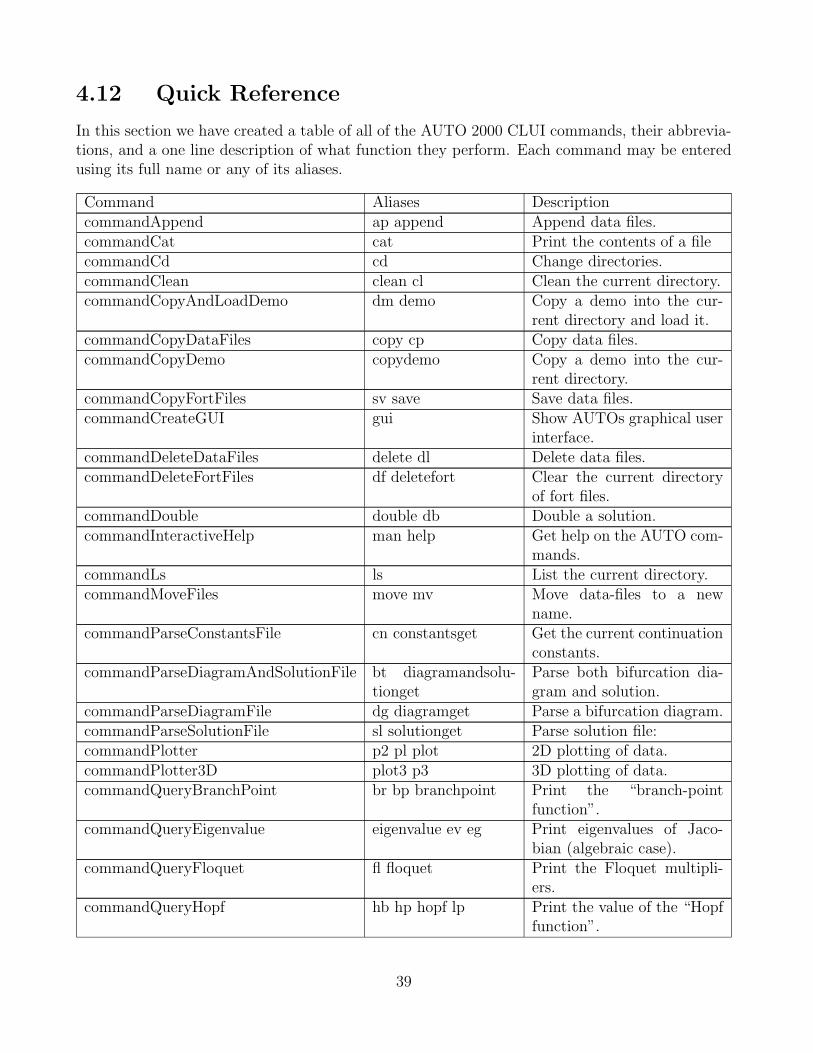
4.12 Quick Reference
In this section we have created a table of all of the AUTO 2000 CLUI commands, their abbrevia-tions, and a one line description of what function they perform. Each command may be enteredusing its full name or any of its aliases.
Command Aliases DescriptioncommandAppend ap append Append data files.commandCat cat Print the contents of a filecommandCd cd Change directories.commandClean clean cl Clean the current directory.commandCopyAndLoadDemo dm demo Copy a demo into the cur-
rent directory and load it.commandCopyDataFiles copy cp Copy data files.commandCopyDemo copydemo Copy a demo into the cur-
rent directory.commandCopyFortFiles sv save Save data files.commandCreateGUI gui Show AUTOs graphical user
interface.commandDeleteDataFiles delete dl Delete data files.commandDeleteFortFiles df deletefort Clear the current directory
of fort files.commandDouble double db Double a solution.commandInteractiveHelp man help Get help on the AUTO com-
mands.commandLs ls List the current directory.commandMoveFiles move mv Move data-files to a new
name.commandParseConstantsFile cn constantsget Get the current continuation
tiongetParse both bifurcation dia-gram and solution.
commandParseDiagramFile dg diagramget Parse a bifurcation diagram.commandParseSolutionFile sl solutionget Parse solution file:commandPlotter p2 pl plot 2D plotting of data.commandPlotter3D plot3 p3 3D plotting of data.commandQueryBranchPoint br bp branchpoint Print the “branch-point
function”.commandQueryEigenvalue eigenvalue ev eg Print eigenvalues of Jaco-
bian (algebraic case).commandQueryFloquet fl floquet Print the Floquet multipli-
ers.commandQueryHopf hb hp hopf lp Print the value of the “Hopf
function”.
39
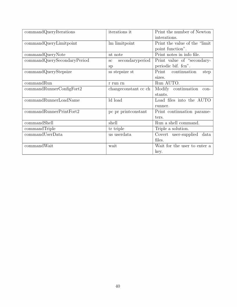
commandQueryIterations iterations it Print the number of Newtoninterations.
commandQueryLimitpoint lm limitpoint Print the value of the “limitpoint function”.
commandQueryNote nt note Print notes in info file.commandQuerySecondaryPeriod sc secondaryperiod
spPrint value of “secondary-periodic bif. fcn”.
commandQueryStepsize ss stepsize st Print continuation stepsizes.
commandRun r run rn Run AUTO.commandRunnerConfigFort2 changeconstant cc ch Modify continuation con-
stants.commandRunnerLoadName ld load Load files into the AUTO
runner.commandRunnerPrintFort2 pc pr printconstant Print continuation parame-
ters.commandShell shell Run a shell command.commandTriple tr triple Triple a solution.commandUserData us userdata Covert user-supplied data
files.commandWait wait Wait for the user to enter a
key.
40
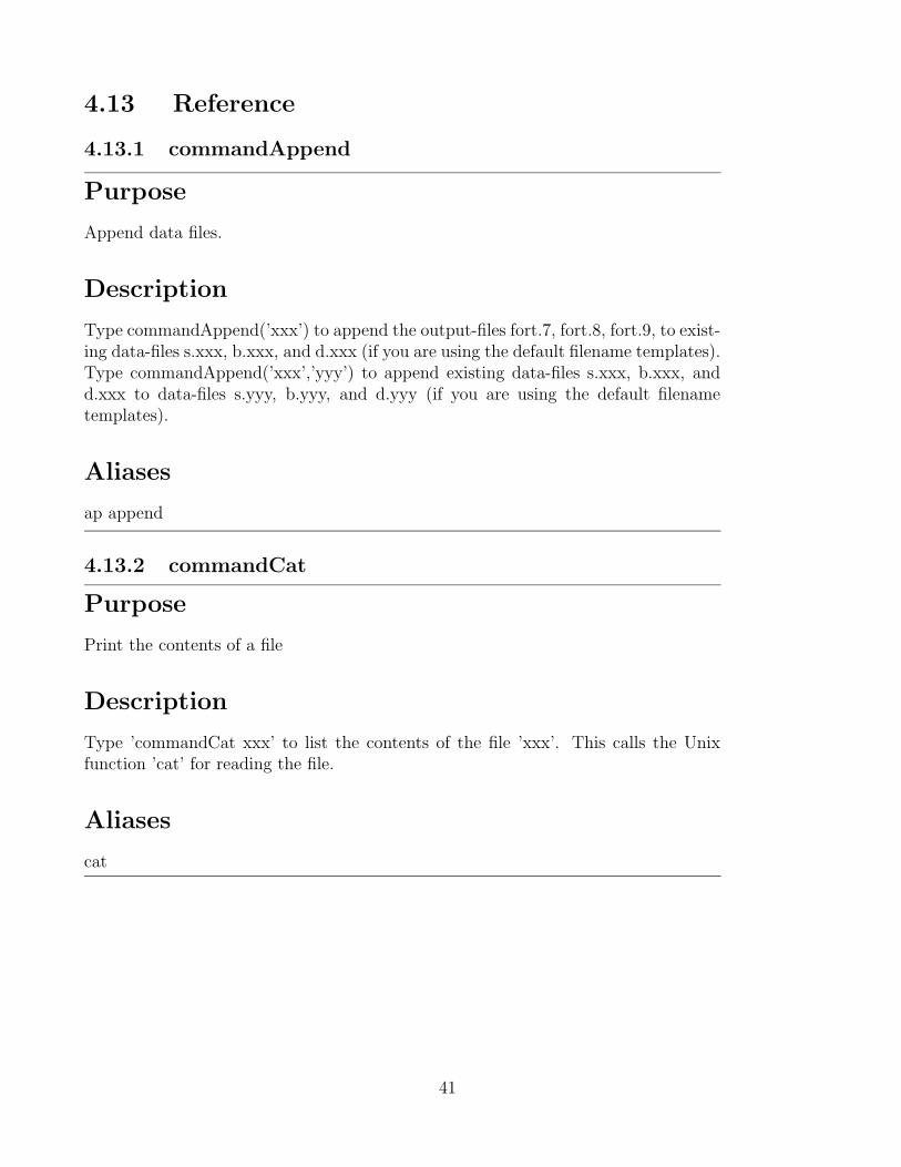
4.13 Reference
4.13.1 commandAppend
Purpose
Append data files.
Description
Type commandAppend(’xxx’) to append the output-files fort.7, fort.8, fort.9, to exist-ing data-files s.xxx, b.xxx, and d.xxx (if you are using the default filename templates).Type commandAppend(’xxx’,’yyy’) to append existing data-files s.xxx, b.xxx, andd.xxx to data-files s.yyy, b.yyy, and d.yyy (if you are using the default filenametemplates).
Aliases
ap append
4.13.2 commandCat
Purpose
Print the contents of a file
Description
Type ’commandCat xxx’ to list the contents of the file ’xxx’. This calls the Unixfunction ’cat’ for reading the file.
Aliases
cat
41
4.13.3 commandCd
Purpose
Change directories.
Description
Type ’commandCd xxx’ to change to the directory ’xxx’. This command understandsboth shell variables and home directory expansion.
Aliases
cd
4.13.4 commandClean
Purpose
Clean the current directory.
Description
Type commandClean() to clean the current directory. This command will delete allfiles of the form fort.*, *.o, and *.exe.
Aliases
clean cl
42
4.13.5 commandCopyAndLoadDemo
Purpose
Copy a demo into the current directory and load it.
Description
Type commandCopyAndLoadDemo(’xxx’) to copy all files fromauto/2000/demos/xxx to the current user directory. Here ’xxx’ denotes ademo name; e.g., ’abc’. Note that the ’dm’ command also copies a Makefile tothe current user directory. To avoid the overwriting of existing files, always rundemos in a clean work directory. NOTE: This command automatically performs thecommandRunnerLoadName command as well.
Aliases
dm demo
4.13.6 commandCopyDataFiles
Purpose
Copy data files.
Description
Type commandCopyDataFiles(’xxx’,’yyy’) to copy the data-files c.xxx, d.xxx, b.xxx,and h.xxx to c.yyy, d.yyy, b.yyy, and h.yyy (if you are using the default filenametemplates).
Aliases
copy cp
43
4.13.7 commandCopyDemo
Purpose
Copy a demo into the current directory.
Description
Type commandCopyDemo(’xxx’) to copy all files from auto/2000/demos/xxx to thecurrent user directory. Here ’xxx’ denotes a demo name; e.g., ’abc’. Note that the’dm’ command also copies a Makefile to the current user directory. To avoid theoverwriting of existing files, always run demos in a clean work directory.
Aliases
copydemo
4.13.8 commandCopyFortFiles
Purpose
Save data files.
Description
Type commandCopyFortFiles(’xxx’) to save the output-files fort.7, fort.8, fort.9, tob.xxx, s.xxx, d.xxx (if you are using the default filename templates). Existing fileswith these names will be overwritten.
Aliases
sv save
44
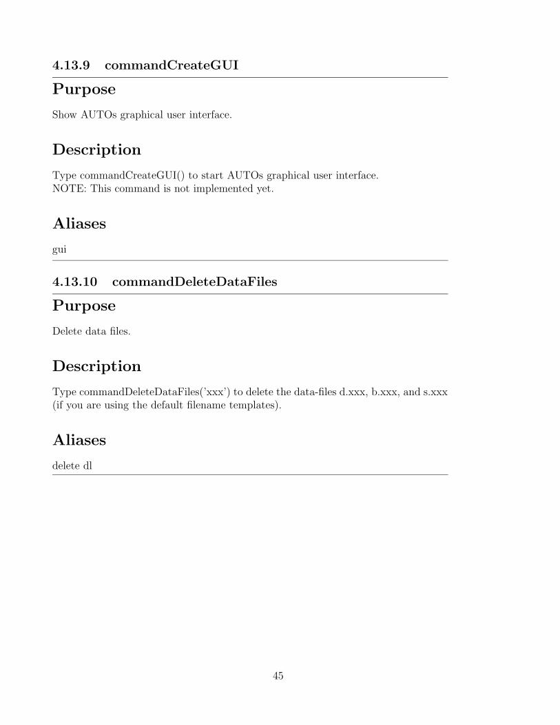
4.13.9 commandCreateGUI
Purpose
Show AUTOs graphical user interface.
Description
Type commandCreateGUI() to start AUTOs graphical user interface.NOTE: This command is not implemented yet.
Aliases
gui
4.13.10 commandDeleteDataFiles
Purpose
Delete data files.
Description
Type commandDeleteDataFiles(’xxx’) to delete the data-files d.xxx, b.xxx, and s.xxx(if you are using the default filename templates).
Aliases
delete dl
45
4.13.11 commandDeleteFortFiles
Purpose
Clear the current directory of fort files.
Description
Type commandDeleteFortFiles() to clean the current directory. This command willdelete all files of the form fort.*.
Aliases
df deletefort
4.13.12 commandDouble
Purpose
Double a solution.
Description
Type commandDouble() to double the solution in ’fort.7’ and ’fort.8’.Type commandDouble(’xxx’) to double the solution in b.xxx and s.xxx (if you areusing the default filename templates).
Aliases
double db
46
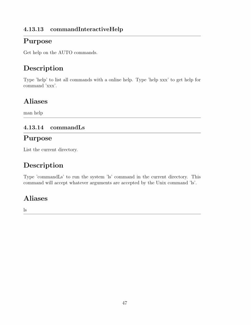
4.13.13 commandInteractiveHelp
Purpose
Get help on the AUTO commands.
Description
Type ’help’ to list all commands with a online help. Type ’help xxx’ to get help forcommand ’xxx’.
Aliases
man help
4.13.14 commandLs
Purpose
List the current directory.
Description
Type ’commandLs’ to run the system ’ls’ command in the current directory. Thiscommand will accept whatever arguments are accepted by the Unix command ’ls’.
Aliases
ls
47
4.13.15 commandMoveFiles
Purpose
Move data-files to a new name.
Description
Type commandMoveFiles(’xxx’,’yyy’) to move the data-files b.xxx, s.xxx, d.xxx, andc.xxx to b.yyy, s.yyy, d.yyy, and c.yyy (if you are using the default filename tem-plates).
Aliases
move mv
4.13.16 commandParseConstantsFile
Purpose
Get the current continuation constants.
Description
Type commandParseConstantsFile(’xxx’) to get a parsed version of the constants filec.xxx (if you are using the default filename templates).
Aliases
cn constantsget
48
4.13.17 commandParseDiagramAndSolutionFile
Purpose
Parse both bifurcation diagram and solution.
Description
Type commandParseDiagramAndSolutionFile(’xxx’) to get a parsed version of thediagram file b.xxx and solution file s.xxx (if you are using the default filename tem-plates).
Aliases
bt diagramandsolutionget
4.13.18 commandParseDiagramFile
Purpose
Parse a bifurcation diagram.
Description
Type commandParseDiagramFile(’xxx’) to get a parsed version of the diagram fileb.xxx (if you are using the default filename templates).
Aliases
dg diagramget
49
4.13.19 commandParseSolutionFile
Purpose
Parse solution file:
Description
Type commandParseSolutionFile(’xxx’) to get a parsed version of the solution files.xxx (if you are using the default filename templates).
Aliases
sl solutionget
4.13.20 commandPlotter
Purpose
2D plotting of data.
Description
Type commandPlotter(’xxx’) to run the graphics program for the graphical inspectionof the data-files b.xxx and s.xxx (if you are using the default filename templates).The return value will be the handle for the graphics window.Type commandPlotter() to run the graphics program for the graphical inspectionof the output-files ’fort.7’ and ’fort.8’. The return value will be the handle for thegraphics window.
Aliases
p2 pl plot
50
4.13.21 commandPlotter3D
Purpose
3D plotting of data.
Description
Type commandPlotter3D(’xxx’) to run the graphics program for the graphical inspec-tion of the data-files b.xxx and s.xxx (if you are using the default filename templates).The return value will be the handle for the graphics window.Type commandPlotter3D() to run the graphics program for the graphical inspectionof the output-files ’fort.7’ and ’fort.8’. The return value will be the handle for thegraphics window.
Aliases
plot3 p3
4.13.22 commandQueryBranchPoint
Purpose
Print the “branch-point function”.
Description
Type commandQueryBranchPoint() to list the value of the “branch-point function”in the output-file fort.9. This function vanishes at a branch point.Type commandQueryBranchPoint(’xxx’) to list the value of the “branch-point func-tion” in the info file ’d.xxx’.
Aliases
br bp branchpoint
51
4.13.23 commandQueryEigenvalue
Purpose
Print eigenvalues of Jacobian (algebraic case).
Description
Type commandQueryEigenvalue() to list the eigenvalues of the Jacobian in fort.9.(Algebraic problems.)Type commandQueryEigenvalue(’xxx’) to list the eigenvalues of the Jacobian in theinfo file ’d.xxx’.
Aliases
eigenvalue ev eg
4.13.24 commandQueryFloquet
Purpose
Print the Floquet multipliers.
Description
Type commandQueryFloquet() to list the Floquet multipliers in the output-file fort.9.(Differential equations.)Type commandQueryFloquet(’xxx’) to list the Floquet multipliers in the info file’d.xxx’.
Aliases
fl floquet
52
4.13.25 commandQueryHopf
Purpose
Print the value of the “Hopf function”.
Description
Type commandQueryHopf() to list the value of the “Hopf function” in the output-filefort.9. This function vanishes at a Hopf bifurcation point.Type commandQueryHopf(’xxx’) to list the value of the “Hopf function” in the infofile ’d.xxx’.
Aliases
hb hp hopf lp
4.13.26 commandQueryIterations
Purpose
Print the number of Newton interations.
Description
Type commandQueryIterations() to list the number of Newton iterations per contin-uation step in fort.9.Type commandQueryIterations(’xxx’) to list the number of Newton iterations percontinuation step in the info file ’d.xxx’.
Aliases
iterations it
53
4.13.27 commandQueryLimitpoint
Purpose
Print the value of the “limit point function”.
Description
Type commandQueryLimitpoint() to list the value of the “limit point function” inthe output-file fort.9. This function vanishes at a limit point (fold).Type commandQueryLimitpoint(’xxx’) to list the value of the “limit point function”in the info file ’d.xxx’.
Aliases
lm limitpoint
4.13.28 commandQueryNote
Purpose
Print notes in info file.
Description
Type commandQueryNote() to show any notes in the output-file fort.9.Type commandQueryNote(’xxx’) to show any notes in the info file ’d.xxx’.
Aliases
nt note
54
4.13.29 commandQuerySecondaryPeriod
Purpose
Print value of “secondary-periodic bif. fcn”.
Description
Type commandQuerySecondaryPeriod() to list the value of the “secondary-periodicbifurcation function” in the output-file ’fort.9. This function vanishes at period-doubling and torus bifurcations.Type commandQuerySecondaryPeriod(’xxx’) to list the value of the “secondary-periodic bifurcation function” in the info file ’d.xxx’.
Aliases
sc secondaryperiod sp
4.13.30 commandQueryStepsize
Purpose
Print continuation step sizes.
Description
Type commandQueryStepsize() to list the continuation step size for each continuationstep in ’fort.9.Type commandQueryStepsize(’xxx’) to list the continuation step size for each con-tinuation step in the info file ’d.xxx’.
Aliases
ss stepsize st
55
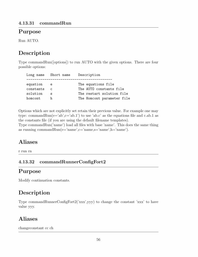
4.13.31 commandRun
Purpose
Run AUTO.
Description
Type commandRun([options]) to run AUTO with the given options. There are fourpossible options:
Long name Short name Description
-------------------------------------------
equation e The equations file
constants c The AUTO constants file
solution s The restart solution file
homcont h The Homcont parameter file
Options which are not explicitly set retain their previous value. For example one maytype: commandRun(e=’ab’,c=’ab.1’) to use ’ab.c’ as the equations file and c.ab.1 asthe constants file (if you are using the default filename templates).Type commandRun(’name’) load all files with base ’name’. This does the same thingas running commandRun(e=’name’,c=’name,s=’name’,h=’name’).
Aliases
r run rn
4.13.32 commandRunnerConfigFort2
Purpose
Modify continuation constants.
Description
Type commandRunnerConfigFort2(’xxx’,yyy) to change the constant ’xxx’ to havevalue yyy.
Aliases
changeconstant cc ch
56
4.13.33 commandRunnerLoadName
Purpose
Load files into the AUTO runner.
Description
Type commandRunnerLoadName([options]) to modify AUTO runner. There are fourpossible options:
Long name Short name Description
-------------------------------------------
equation e The equations file
constants c The AUTO constants file
solution s The restart solution file
homcont h The Homcont parameter file
Options which are not explicitly set retain their previous value. For example one maytype: commandRunnerLoadName(e=’ab’,c=’ab.1’) to use ’ab.c’ as the equations fileand c.ab.1 as the constants file (if you are using the default filename templates).Type commandRunnerLoadName(’name’) load all files with base’name’. This does the same thing as running commandRunnerLoad-Name(e=’name’,c=’name,s=’name’,h=’name’).
Aliases
ld load
57
4.13.34 commandRunnerPrintFort2
Purpose
Print continuation parameters.
Description
Type commandRunnerPrintFort2() to print all the parameters. Type commandRun-nerPrintFort2(’xxx’) to return the parameter ’xxx’.
Aliases
pc pr printconstant
4.13.35 commandShell
Purpose
Run a shell command.
Description
Type ’shell xxx’ to run the command ’xxx’ in the Unix shell and display the resultsin the AUTO command line user interface.
Aliases
shell
58
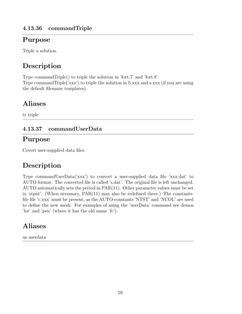
4.13.36 commandTriple
Purpose
Triple a solution.
Description
Type commandTriple() to triple the solution in ’fort.7’ and ’fort.8’.Type commandTriple(’xxx’) to triple the solution in b.xxx and s.xxx (if you are usingthe default filename templates).
Aliases
tr triple
4.13.37 commandUserData
Purpose
Covert user-supplied data files.
Description
Type commandUserData(’xxx’) to convert a user-supplied data file ’xxx.dat’ toAUTO format. The converted file is called ’s.dat’. The original file is left unchanged.AUTO automatically sets the period in PAR(11). Other parameter values must be setin ’stpnt’. (When necessary, PAR(11) may also be redefined there.) The constants-file file ’c.xxx’ must be present, as the AUTO-constants ’NTST’ and ’NCOL’ are usedto define the new mesh. For examples of using the ’userData’ command see demos’lor’ and ’pen’ (where it has the old name ’fc’).
Aliases
us userdata
59
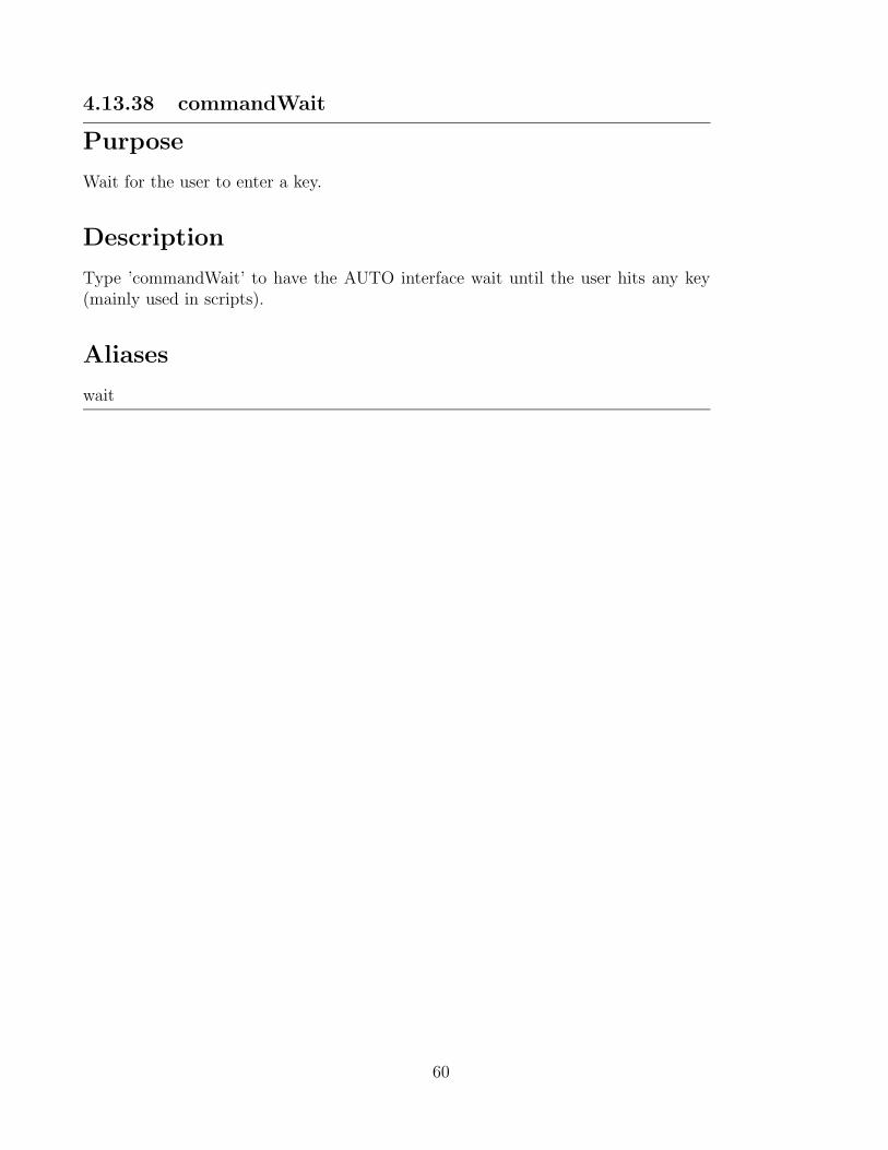
4.13.38 commandWait
Purpose
Wait for the user to enter a key.
Description
Type ’commandWait’ to have the AUTO interface wait until the user hits any key(mainly used in scripts).
Aliases
wait
60
Chapter 5
Description of AUTO -Constants.
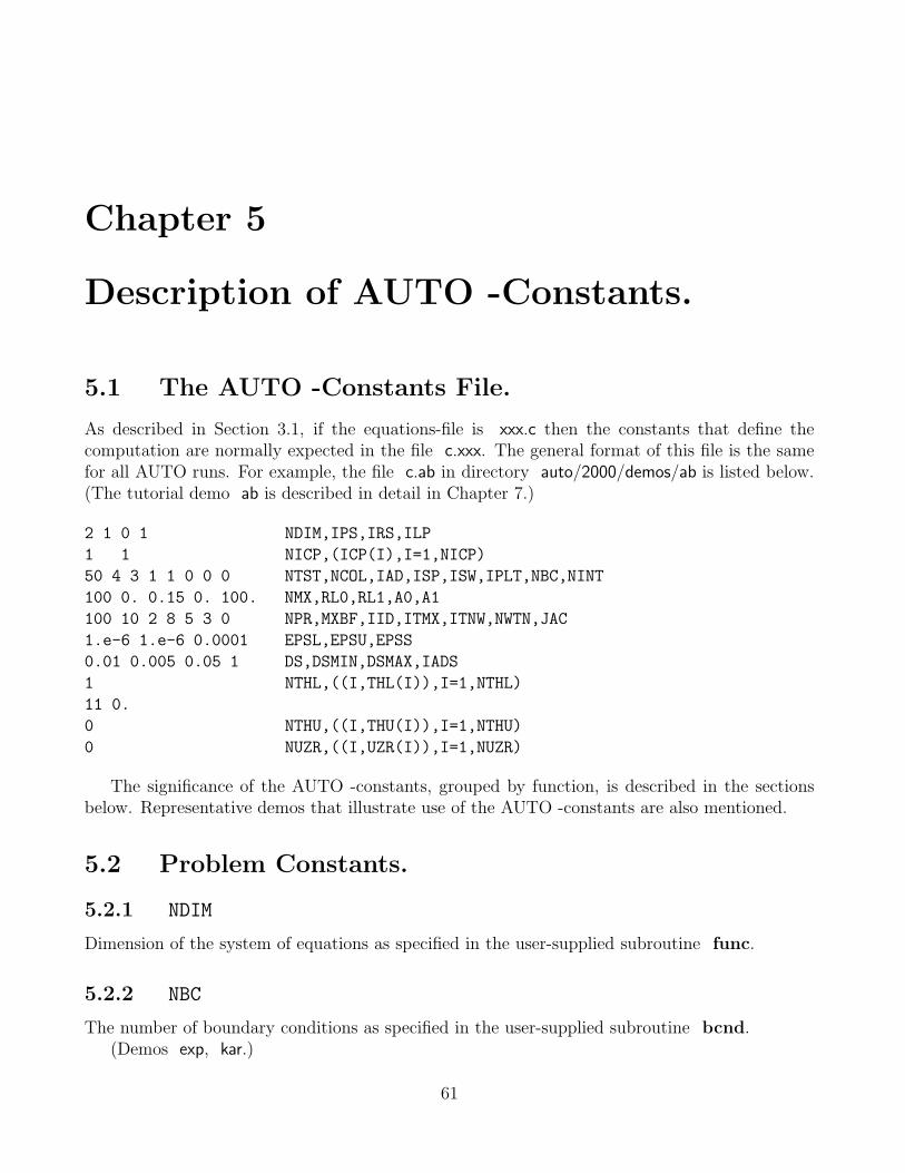
5.1 The AUTO -Constants File.
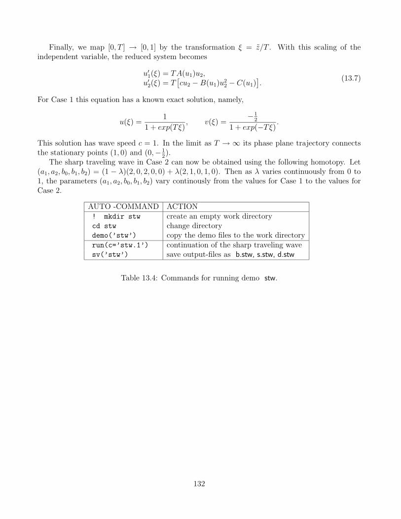
As described in Section 3.1, if the equations-file is xxx.c then the constants that define thecomputation are normally expected in the file c.xxx. The general format of this file is the samefor all AUTO runs. For example, the file c.ab in directory auto/2000/demos/ab is listed below.(The tutorial demo ab is described in detail in Chapter 7.)
The significance of the AUTO -constants, grouped by function, is described in the sectionsbelow. Representative demos that illustrate use of the AUTO -constants are also mentioned.
5.2 Problem Constants.
5.2.1 NDIM
Dimension of the system of equations as specified in the user-supplied subroutine func.
5.2.2 NBC
The number of boundary conditions as specified in the user-supplied subroutine bcnd.(Demos exp, kar.)
61
5.2.3 NINT
The number of integral conditions as specified in the user-supplied subroutine icnd.(Demos int, lin, obv.)
5.2.4 JAC
Used to indicate whether derivatives are supplied by the user or to be obtained by differencing :
- JAC=0 : No derivatives are given by the user. (Most demos use JAC=0.)
- JAC=1 : Derivatives with respect to state- and problem-parameters are given in the user-supplied subroutines func, bcnd, icnd and fopt, where applicable. This may be neces-sary for sensitive problems. It is also recommended for computations in which AUTO gen-erates an extended system, for example, when ISW=2.
(Demos int, dd2, obt, plp, ops.)
(For ISW see Section 5.8.3.)
5.3 Discretization Constants.
5.3.1 NTST
The number of mesh intervals used for discretization. NTST remains fixed during any particularrun, but can be changed when restarting. Recommended value of NTST : As small as possible tomaintain convergence.
(Demos exp, ab, spb.)(For mesh adaption see IAD in Section 5.3.3.)
5.3.2 NCOL
The number of Gauss collocation points per mesh interval, (2 ≤ NCOL ≤ 7). NCOL remains fixedduring any given run, but can be changed when restarting at a previously computed solution.The choice NCOL=4, used in most demos, is recommended. If NDIM is “large” and the solutions“very smooth” then NCOL=2 may be appropriate.
5.3.3 IAD
This constant controls the mesh adaption :
- IAD=0 : Fixed mesh. Normally, this choice should never be used, as it may result in spurioussolutions. (Demo ext.)
- IAD>0 : Adapt the mesh every IAD steps along the branch. Most demos use IAD=3, whichis the strongly recommended value.
62
When computing “trivial” solutions to a boundary value problem, for example, when allsolution components are constant, then the mesh adaption may fail under certain circumstances,and overflow may occur. In such case, try recomputing the solution branch with a fixed mesh(IAD=0). Be sure to set IAD back to IAD=3 for computing eventual non-trivial bifurcatingsolution branches.
5.4 Tolerances.
5.4.1 EPSL
Relative convergence criterion for equation parameters in the Newton/Chord method. Mostdemos use EPSL=10−6 or EPSL=10−7, which is the recommended value range.
5.4.2 EPSU
Relative convergence criterion for solution components in the Newton/Chord method. Mostdemos use EPSU=10−6 or EPSU=10−7, which is the recommended value range.
5.4.3 EPSS
Relative arclength convergence criterion for the detection of special solutions. Most demos useEPSS=10−4 or EPSS=10−5, which is the recommended value range. Generally, EPSS should beapproximately 100 to 1000 times the value of EPSL, EPSU.
5.4.4 ITMX
The maximum number of iterations allowed in the accurate location of special solutions, suchas bifurcations, folds, and user output points, by Muller’s method with bracketing. The recom-mended value is ITMX=8, used in most demos.
5.4.5 NWTN
After NWTN Newton iterations the Jacobian is frozen, i.e., AUTO uses full Newton for the firstNWTN iterations and the Chord method for iterations NWTN+1 to ITNW. The choice NWTN=3is strongly recommended and used in most demos. Note that this constant is only effective forODEs, i.e., for solving the piecewise polynomial collocation equations. For algebraic systemsAUTO always uses full Newton.
5.4.6 ITNW
The maximum number of combined Newton-Chord iterations. When this maximum is reached,the step will be retried with half the stepsize. This is repeated until convergence, or until theminimum stepsize is reached. In the latter case the computation of the branch is discontinuedand a message printed in fort.9. The recommended value is ITNW=5, but ITNW=7 may be usedfor “difficult” problems, for example, demos spb, chu, plp, etc.
63
5.5 Continuation Step Size.
5.5.1 DS
AUTO uses pseudo-arclength continuation for following solution branches. The pseudo-arclengthstepsize is the distance between the current solution and the next solution on a branch. Bydefault, this distance includes all state variables (or state functions) and all free parameters. Theconstant DS defines the pseudo-arclength stepsize to be used for the first attempted step alongany branch. (Note that if IADS>0 then DS will automatically be adapted for subsequent stepsand for failed steps.) DS may be chosen positive or negative; changing its sign reverses thedirection of computation. The relation DSMIN ≤ | |DS ≤ DSMAX must be satisfied. The precisechoice of DS is problem-dependent; the demos use a value that was found appropriate after someexperimentation.
5.5.2 DSMIN
This is minimum allowable absolute value of the pseudo-arclength stepsize. DSMIN must bepositive. It is only effective if the pseudo-arclength step is adaptive, i.e., if IADS>0. The choiceof DSMIN is highly problem-dependent; most demos use a value that was found appropriate aftersome experimentation. See also the discussion in Section 6.2.
5.5.3 DSMAX
The maximum allowable absolute value of the pseudo-arclength stepsize. DSMAX must be pos-itive. It is only effective if the pseudo-arclength step is adaptive, i.e., if IADS>0. The choiceof DSMAX is highly problem-dependent; most demos use a value that was found appropriate aftersome experimentation. See also the discussion in Section 6.2.
5.5.4 IADS
This constant controls the frequency of adaption of the pseudo-arclength stepsize.
- IADS=0 : Use fixed pseudo-arclength stepsize, i.e., the stepsize will be equal to the specifiedvalue of DS for every step. The computation of a branch will be discontinued as soon asthe maximum number of iterations ITNW is reached. This choice is not recommended.
(Demo tim.)
- IADS>0 : Adapt the pseudo-arclength stepsize after every IADS steps. If the New-ton/Chord iteration converges rapidly then | |DS will be increased, but never beyondDSMAX. If a step fails then it will be retried with half the stepsize. This will be donerepeatedly until the step is successful or until | |DS reaches DSMIN. In the latter case non-convergence will be signalled. The strongly recommended value is IADS=1, which is usedin almost all demos.
64
5.5.5 NTHL
By default, the pseudo-arclength stepsize includes all state variables (or state functions) and allfree parameters. Under certain circumstances one may want to modify the weight accorded toindividual parameters in the definition of stepsize. For this purpose, NTHL defines the number ofparameters whose weight is to be modified. If NTHL=0 then all weights will have default value1.0 . If NTHL>0 then one must enter NTHL pairs, Parameter Index Weight , with each pair ona separate line.
For example, for the computation of periodic solutions it is recommended that the periodnot be included in the pseudo-arclength continuation stepsize, in order to avoid period-inducedlimitations on the stepsize near orbits of infinite period. This exclusion can be accomplished bysetting NTHL=1, with, on a separate line, the pair 11 0.0 . Most demos that compute periodicsolutions use this option; see for example demo ab.
5.5.6 NTHU
Under certain circumstances one may want to modify the weight accorded to individual statevariables (or state functions) in the definition of stepsize. For this purpose, NTHU defines thenumber of states whose weight is to be modified. If NTHU=0 then all weights will have defaultvalue 1.0 . If NTHU>0 then one must enter NTHU pairs, State Index Weight , with each pairon a separate line. At present none of the demos use this option.
5.6 Diagram Limits.
There are three ways to limit the computation of a branch :
- By appropriate choice of the computational window defined by the constants RL0, RL1,A0, and A1. One should always check that the starting solution lies within this computa-tional window, otherwise the computation will stop immediately at the starting point.
- By specifying the maximum number of steps, NMX.
- By specifying a negative parameter index in the list associated with the constant NUZR;see Section 5.9.4.
5.6.1 NMX
The maximum number of steps to be taken along any branch.
5.6.2 RL0
The lower bound on the principal continuation parameter. (This is the parameter which appearsfirst in the ICP list; see Section 5.7.1.).
65
5.6.3 RL1
The upper bound on the principal continuation parameter.
5.6.4 A0
The lower bound on the principal solution measure. (By default, if IPLT=0, the principal solutionmeasure is the L2-norm of the state vector or state vector function. See the AUTO -constantIPLT in Section 5.9.3 for choosing another principal solution measure.)
5.6.5 A1
The upper bound on the principal solution measure.
5.7 Free Parameters.
5.7.1 NICP, ICP
For each equation type and for each continuation calculation there is a typical (“generic”) numberof problem parameters that must be allowed to vary, in order for the calculations to be properlyposed. The constant NICP indicates how many free parameters have been specified, while thearray ICP actually designates these free parameters. The parameter that appears first in theICP list is called the “principal continuation parameter”. Specific examples and special cases aredescribed below.
5.7.2 Fixed points.
The simplest case is the continuation of a solution branch to the system f(u, p) = 0, wheref(·, ·), u ∈ Rn, cf. Equation (2.1). Such a system arises in the continuation of ODE stationarysolutions and in the continuation of fixed points of discrete dynamical systems. There is only onefree parameter here, so NICP=1.
As a concrete example, consider Run 1 of demo ab, where NICP=1, with ICP(1)=1. Thus,in this run PAR(1) is designated as the free parameter.
5.7.3 Periodic solutions and rotations.
The continuation of periodic solutions and rotations generically requires two parameters, namely,one problem parameter and the period. Thus, in this case NICP=2. For example, in Run 2of demo ab we have NICP=2, with ICP(1)=1 and ICP(2)=11. Thus, in this run, the freeparameters are PAR(1) and PAR(11). (Note that AUTO reserves PAR(11) for the period.)
Actually, for periodic solutions, one can set NICP=1 and only specify the index of the freeproblem parameter, as AUTO will automatically addd PAR(11). However, in this case the periodwill not appear in the screen output and in the fort.7 output-file.
For fixed period orbits one must set NICP=2 and specify two free problem parameters. Forexample, in Run 7 of demo pp2, we have NICP=2, with PAR(1) and PAR(2) specified as free
66
problem parameters. The period PAR(11) is fixed in this run. If the period is large then such acontinuation provides a simple and effective method for computing a locus of homoclinic orbits.
5.7.4 Folds and Hopf bifurcations.
The continuation of folds for algebraic problems and the continuation of Hopf bifurcations requirestwo free problem parameters, i.e., NICP=2. For example, to continue a fold in Run 3 of demoab, we have NICP=2, with PAR(1) and PAR(3) specified as free parameters. Note that onemust set ISW=2 for computing such loci of special solutions. Also note that in the continuationof folds the principal continuation parameter must be the one with respect to which the fold waslocated.
5.7.5 Folds and period-doublings.
The continuation of folds, for periodic orbits and rotations, and the continuation of period-doubling bifurcations require two free problem parameters plus the free period. Thus, one wouldnormally set NICP=3. For example, in Run 6 of demo pen, where a locus of period-doublingbifurcations is computed for rotations, we have NICP=3, with PAR(2), PAR(3), and PAR(11)
specified as free parameters. Note that one must set ISW=2 for computing such loci of specialsolutions. Also note that in the continuation of folds the principal continuation parameter mustbe the one with respect to which the fold was located.
Actually, one may set NICP=2, and only specify the problem parameters, as AUTO willautomatically add the period. For example, in Run 3 of demo plp, where a locus of folds iscomputed for periodic orbits, we have NICP=2, with PAR(4) and PAR(1) specified as freeparameters. However, in this case the period will not appear in the screen output and in thefort.7 output-file.
To continue a locus of folds or period-doublings with fixed period, simply set NICP=3 andspecify three problem parameters, not including PAR(11).
5.7.6 Boundary value problems.
The simplest case is that of boundary value problems where NDIM= NBC and where NINT=0.Then, generically, one free problem parameter is required for computing a solution branch. Forexample, in demo exp, we have NDIM= NBC=2, NINT=0. Thus NICP=1. Indeed, in this demoone free parameter is designated, namely PAR(1).
More generally, for boundary value problems with integral constraints, the generic numberof free parameters is NBC + NINT− NDIM +1. For example, in demo lin, we have NDIM=2,NBC=2, and NINT=1. Thus NICP=2. Indeed, in this demo two free parameters are designated,namely PAR(1) and PAR(3).
5.7.7 Boundary value folds.
To continue a locus of folds for a general boundary value problem with integral constraints, setNICP= NBC+ NINT− NDIM+2, and specify this number of parameter indices to designate the freeparameters.
67
5.7.8 Optimization problems.
In algebraic optimization problems one must set ICP(1)=10, as AUTO uses PAR(10) as principalcontinuation parameter to monitor the value of the objective function. Furthermore, one mustdesignate one free equation parameter in ICP(2). Thus, NICP=2 in the first run.
Folds with respect to PAR(10) correspond to extrema of the objective function. In a secondrun one can restart at such a fold, with an additional free equation parameter specified in ICP(3).Thus, NICP=3 in the second run.
The above procedure can be repeated. For example, folds from the second run can be continuedin a third run with three equation parameters specified in addition to PAR(10). Thus, NICP=4in the third run.
For a simple example see demo opt, where a four-parameter extremum is located. Notethat NICP=5 in each of the four constants-files of this demo, with the indices of PAR(10) andPAR(1)-PAR(4) specified in ICP. Thus, in the first three runs, there are overspecified parameters.However, AUTO will always use the correct number of parameters. Although the overspecifiedparameters will be printed, their values will remain fixed.
5.7.9 Internal free parameters.
The actual continuation scheme in AUTO may use additional free parameters that are automati-cally added. The simplest example is the computation of periodic solutions and rotations, whereAUTO automatically adds the period, if not specified. The computation of loci of folds, Hopf bi-furcations, and period-doublings also requires additional internal continuation parameters. Thesewill be automatically added, and their indices will be greater than 10.
5.7.10 Parameter overspecification.
The number of specified parameter indices is allowed to be be greater than the generic number.In such case there will be “overspecified” parameters, whose values will appear in the screen andfort.7 output, but which are not part of the continuation process. A simple example is providedby demo opt, where the first three runs have overspecified parameters whose values, althoughconstant, are printed.
There is, however, a more useful application of parameter overspecification. In the user-supplied subroutine pvls one can define solution measures and assign these to otherwise unusedparameters. Such parameters can then be overspecified, in order to print them on the screen andin the fort.7 output. It is important to note that such overspecified parameters must appear atthe end of the ICP list, as they cannot be used as true continuation parameters.
For an example of using parameter overspecification for printing user-defined solution mea-sures, see demo pvl. This is a boundary value problem (Bratu’s equation) which has only onetrue continuation parameter, namely PAR(1). Three solution measures are defined in the sub-routine pvls, namely, the L2-norm of the first solution component, the minimum of the secondcomponent, and the left boundary value of the second component. These solution measures areassigned to PAR(2), PAR(3), and PAR(4), respectively. In the constants-file c.pvl we haveNICP=4, with PAR(1)-PAR(4) specified as parameters. Thus, in this example, PAR(2)-PAR(4)
68
are overspecified. Note that PAR(1) must appear first in the ICP list; the other parameterscannot be used as true continuation parameters.
5.8 Computation Constants.
5.8.1 ILP
- ILP=0 : No detection of folds. This choice is recommended.
- ILP=1 : Detection of folds. To be used if subsequent fold continuation is intended.
2
5.8.2 ISP
This constant controls the detection of branch points, period-doubling bifurcations, and torusbifurcations.
- ISP=0 : This setting disables the detection of branch points, period-doubling bifurcations,and torus bifurcations and the computation of Floquet multipliers.
- ISP=1 : Branch points are detected for algebraic equations, but not for periodic solutionsand boundary value problems. Period-doubling bifurcations and torus bifurcations are notlocated either. However, Floquet multipliers are computed.
- ISP=2 : This setting enables the detection of all special solutions. For periodic solutionsand rotations, the choice ISP=2 should be used with care, due to potential inaccuracy inthe computation of the linearized Poincare map and possible rapid variation of the Floquetmultipliers. The linearized Poincare map always has a multiplier z = 1. If this multiplierbecomes inaccurate then the automatic detection of secondary periodic bifurcations will bediscontinued and a warning message will be printed in fort.9. See also Section 6.4.
- ISP=3 : Branch points will be detected, but AUTO will not monitor the Floquet multipliers.Period-doubling and torus bifurcations will go undetected. This option is useful for certainproblems with non-generic Floquet behavior. The Floquet multipliers will be output to thediagnostic file.
5.8.3 ISW
This constant controls branch switching at branch points for the case of differential equations.Note that branch switching is automatic for algebraic equations.
- ISW=1 : This is the normal value of ISW.
- ISW=−1 : If IRS is the label of a branch point or a period-doubling bifurcation then branchswitching will be done. For period doubling bifurcations it is recommended that NTST beincreased. For examples see Run 2 and Run 3 of demo lor, where branch switching is done
69
at period-doubling bifurcations, and Run 2 and Run 3 of demo bvp, where branch switchingis done at a transcritical branch point.
- ISW=2 : If IRS is the label of a fold, a Hopf bifurcation point, or a period-doubling or torusbifurcation then a locus of such points will be computed. An additional free parametermust be specified for such continuations; see also Section 5.7.
5.8.4 MXBF
This constant, which is effective for algebraic problems only, sets the maximum number of bifur-cations to be treated. Additional branch points will be noted, but the corresponding bifurcatingbranches will not be computed. If MXBF is positive then the bifurcating branches of the firstMXBF branch points will be traced out in both directions. If MXBF is negative then the bifurcatingbranches of the first | MXBF | branch points will be traced out in only one direction.
5.8.5 IRS
This constant sets the label of the solution where the computation is to be restarted.
- IRS=0 : This setting is typically used in the first run of a new problem. In this case a startingsolution must be defined in the user-supplied subroutine stpnt; see also Section 3.3. Forrepresentative examples of analytical starting solutions see demos ab and frc. For startingfrom unlabeled numerical data see the @fc command (Section A) and demos lor and pen.
- IRS>0 : Restart the computation at the previously computed solution with label IRS.This solution is normally expected to be in the current data-file q.xxx; see also the @r and@R commands in Section A. Various AUTO -constants can be modified when restarting.
5.8.6 IPS
This constant defines the problem type :
- IPS=0 : An algebraic bifurcation problem. Hopf bifurcations will not be detected andstability properties will not be indicated in the fort.7 output-file.
- IPS=1 : Stationary solutions of ODEs with detection of Hopf bifurcations. The sign of PT,the point number, in fort.7 is used to indicate stability : − is stable , + is unstable.
(Demo ab.)
- IPS=−1 : Fixed points of the discrete dynamical system u(k+1) = f(u(k), p), with detectionof Hopf bifurcations. The sign of PT in fort.7 indicates stability : − is stable , + is unstable.(Demo dd2.)
- IPS=−2 : Time integration using implicit Euler. The AUTO -constants DS, DSMIN,DSMAX, and ITNW, NWTN control the stepsize. In fact, pseudo-arclength is used for “con-tinuation in time”. Note that the time discretization is only first order accurate, so thatresults should be carefully interpreted. Indeed, this option has been included primarily
70
for the detection of stationary solutions, which can then be entered in the user-suppliedsubroutine stpnt.
(Demo ivp.)
- IPS=2 : Computation of periodic solutions. Starting data can be a Hopf bifurcation point(Run 2 of demo ab), a periodic orbit from a previous run (Run 4 of demo pp2), ananalytically known periodic orbit (Run 1 of demo frc), or a numerically known periodicorbit (Demo lor). The sign of PT in fort.7 is used to indicate stability : − is stable , + isunstable or unknown.
- IPS=4 : A boundary value problem. Boundary conditions must be specified in the user-supplied subroutine bcnd and integral constraints in icnd. The AUTO -constants NBC
and NINT must be given correct values. (Demos exp, int, kar.)
- IPS=5 : Algebraic optimization problems. The objective function must be specified in theuser-supplied subroutine fopt. (Demo opt.)
- IPS=7 : A boundary value problem with computation of Floquet multipliers. This is avery special option; for most boundary value problems one should use IPS=4. Boundaryconditions must be specified in the user-supplied subroutine bcnd and integral constraintsin icnd. The AUTO -constants NBC and NINT must be given correct values.
- IPS=9 : This option is used in connection with the HomCont algorithms described inChapters 15-21 for the detection and continuation of homoclinic bifurcations.
(Demos san, mtn, kpr, cir, she, rev.)
- IPS=11 : Spatially uniform solutions of a system of parabolic PDEs, with detection oftraveling wave bifurcations. The user need only define the nonlinearity (in subroutine func),initialize the wave speed in PAR(10), initialize the diffusion constants in PAR(15,16,· · ·),and set a free equation parameter in ICP(1). (Run 2 of demo wav.)
- IPS=12 : Continuation of traveling wave solutions to a system of parabolic PDEs. Startingdata can be a Hopf bifurcation point from a previous run with IPS=11, or a traveling wavefrom a previous run with IPS=12. (Run 3 and Run 4 of demo wav.)
- IPS=14 : Time evolution for a system of parabolic PDEs subject to periodic boundaryconditions. Starting data may be solutions from a previous run with IPS=12 or 14. Start-ing data can also be specified in stpnt, in which case the wave length must be specifiedin PAR(11), and the diffusion constants in PAR(15,16,· · ·). AUTO uses PAR(14) forthe time variable. DS, DSMIN, and DSMAX govern the pseudo-arclength continuation inthe space-time variables. Note that the time discretization is only first order accurate, sothat results should be carefully interpreted. Indeed, this option is mainly intended for thedetection of stationary waves. (Run 5 of demo wav.)
- IPS=15 : Optimization of periodic solutions. The integrand of the objective functionalmust be specified in the user-supplied subroutine fopt. Only PAR(1-9) should be usedfor problem parameters. PAR(10) is the value of the objective functional, PAR(11) the
71
period, PAR(12) the norm of the adjoint variables, PAR(14) and PAR(15) are internaloptimality variables. PAR(21-29) and PAR(31) are used to monitor the optimalityfunctionals associated with the problem parameters and the period. Computations can bestarted at a solution computed with IPS=2 or IPS=15. For a detailed example see demoops.
- IPS=16 : This option is similar to IPS=14, except that the user supplies the boundaryconditions. Thus this option can be used for time-integration of parabolic systems subjectto user-defined boundary conditions. For examples see the first runs of demos pd1, pd2,and bru. Note that the space-derivatives of the initial conditions must also be suppliedin the user-supplied subroutine stpnt. The initial conditions must satisfy the boundaryconditions. This option is mainly intended for the detecting stationary solutions.
- IPS=17 : This option can be used to continue stationary solutions of parabolic systemsobtained from an evolution run with IPS=16. For examples see the second runs of demospd1 and pd2.
5.9 Output Control.
5.9.1 NPR
This constant can be used to regularly write fort.8 plotting and restart data. IF NPR>0 thensuch output is written every NPR steps. IF NPR=0 or if NPR≥ NMX then no such output iswritten. Note that special solutions, such as branch points, folds, end points, etc., are alwayswritten in fort.8. Furthermore, one can specify parameter values where plotting and restartdata is to be written; see Section 5.9.4. For these reasons, and to limit the output volume, it isrecommended that NPR output be kept to a minimum.
5.9.2 IID
This constant controls the amount of diagnostic output printed in fort.9 : the greater IID themore detailed the diagnostic output.
- IID=0 : Minimal diagnostic output. This setting is not recommended.
- IID=2 : Regular diagnostic output. This is the recommended value of IID.
- IID=3 : This setting gives additional diagnostic output for algebraic equations, namely theJacobian and the residual vector at the starting point. This information, which is printedat the beginning of fort.9, is useful for verifying whether the starting solution in stpnt isindeed a solution.
- IID=4 : This setting gives additional diagnostic output for differential equations, namelythe reduced system and the associated residual vector. This information is printed for everystep and for every Newton iteration, and should normally be suppressed. In particular itcan be used to verify whether the starting solution is indeed a solution. For this purpose,
72
the stepsize DS should be small, and one should look at the residuals printed in the fort.9output-file. (Note that the first residual vector printed in fort.9 may be identically zero, asit may correspond to the computation of the starting direction. Look at the second residualvector in such case.) This residual vector has dimension NDIM+ NBC+ NINT+1, whichaccounts for the NDIM differential equations, the NBC boundary conditions, the NINT user-defined integral constraints, and the pseudo-arclength equation. For proper interpretationsof these data one may want to refer to the solution algorithm for solving the collocationsystem, as described in Doedel, Keller & Kernevez (1991b).
- IID=5 : This setting gives very extensive diagnostic output for differential equations, namely,debug output from the linear equation solver. This setting should not normally be used asit may result in a huge fort.9 file.
5.9.3 IPLT
This constant allows redefinition of the principal solution measure, which is printed as the second(real) column in the screen output and in the fort.7 output-file :
- If IPLT = 0 then the L2-norm is printed. Most demos use this setting. For algebraicproblems, the standard definition of L2-norm is used. For differential equations, the L2-norm is defined as
√
√
√
√
∫ 1
0
NDIM∑
k=1
Uk(x)2 dx .
Note that the interval of integration is [0, 1], the standard interval used by AUTO. Forperiodic solutions the independent variable is transformed to range from 0 to 1, beforethe norm is computed. The AUTO-constants THL(*) and THU(*) (see Section 5.5.5 andSection 5.5.6) affect the definition of the L2-norm.
- If 0 < IPLT ≤ NDIM then the maximum of the IPLT’th solution component is printed.
- If − NDIM ≤ IPLT <0 then the minimum of the IPLT’th solution component is printed.(Demo fsh.)
- If NDIM < IPLT ≤ 2* NDIM then the integral of the ( IPLT− NDIM)’th solution componentis printed. (Demos exp, lor.)
- If 2* NDIM < IPLT ≤ 3* NDIM then the L2-norm of the ( IPLT− NDIM)’th solution com-ponent is printed. (Demo frc.)
Note that for algebraic problems the maximum and the minimum are identical. Also, forODEs the maximum and the minimum of a solution component are generally much less accuratethan the L2-norm and component integrals. Note also that the subroutine pvls provides asecond, more general way of defining solution measures; see Section 5.7.10.
73
5.9.4 NUZR
This constant allows the setting of parameter values at which labeled plotting and restart infor-mation is to be written in the fort.8 output-file. Optionally, it also allows the computation toterminate at such a point.
- Set NUZR=0 if no such output is needed. Many demos use this setting.
- If NUZR>0 then one must enter NUZR pairs, Parameter-Index Parameter-Value , witheach pair on a separate line, to designate the parameters and the parameter values at whichoutput is to be written. For examples see demos exp, int, and fsh.
- If such a parameter index is preceded by a minus sign then the computation will terminateat such a solution point. (Demos pen and bru.)
Note that fort.8 output can also be written at selected values of overspecified parameters. Foran example see demo pvl. For details on overspecified parameters see Section 5.7.10.
74
Chapter 6
Notes on Using AUTO .
6.1 Restrictions on the Use of PAR.
The array PAR in the user-supplied subroutines is available for equation parameters that theuser wants to vary at some point in the computations. In any particular computation the freeparameter(s) must be designated in ICP; see Section 5.7. The following restrictions apply :
- The maximum number of parameters, NPARX in auto/2000/src/auto c.h, has pre-definedvalue NPARX=36. NPARX should not normally be increased and it should never be de-creased. Any increase of NPARX must be followed by recompilation of AUTO .
- Generally one should only use PAR(1)-PAR(9) for equation parameters, as AUTO mayneed the other components internally.
6.2 Efficiency.
In AUTO , efficiency has at times been sacrificed for generality of programming. This applies inparticular to computations in which AUTO generates an extended system, for example, compu-tations with ISW=2. However, the user has significant control over computational efficiency, inparticular through judicious choice of the AUTO -constants DS, DSMIN, and DSMAX, and, forODEs, NTST and NCOL. Initial experimentation normally suggests appropriate values.
Slowly varying solutions to ODEs can often be computed with remarkably small values ofNTST and NCOL, for example, NTST=5, NCOL=2. Generally, however, it is recommended to setNCOL=4, and then to use the “smallest” value of NTST that maintains convergence.
The choice of the pseudo-arclength stepsize parameters DS, DSMIN, and DSMAX is highlyproblem dependent. Generally, DSMIN should not be taken too small, in order to prevent excessivestep refinement in case of non-convergence. It should also not be too large, in order to avoid instantnon-convergence. DSMAX should be sufficiently large, in order to reduce computation time andamount of output data. On the other hand, it should be sufficiently small, in order to preventstepping over bifurcations without detecting them. For a given equation, appropriate values ofthese constants can normally be found after some initial experimentation.
The constants ITNW, NWTN, THL, EPSU, EPSL, EPSS also affect efficiency. Understandingtheir significance is therefore useful; see Section 5.4 and Section 5.5. Finally, it is recommended
75
that initial computations be done with ILP=0; no fold detection; and ISP=1; no bifurcationdetection for ODEs.
6.3 Correctness of Results.
AUTO -computed solutions to ODEs are almost always structurally correct, because the meshadaption strategy, if IAD>0, safeguards to some extent against spurious solutions. If these dooccur, possibly near infinite-period orbits, the unusual appearance of the solution branch typicallyserves as a warning. Repeating the computation with increased NTST is then recommended.
6.4 Bifurcation Points and Folds.
It is recommended that the detection of folds and bifurcation points be initially disabled. Forexample, if an equation has a “vertical” solution branch then AUTO may try to locate one foldafter another.
Generally, degenerate bifurcations cannot be detected. Furthermore, bifurcations that areclose to each other may not be noticed when the pseudo-arclength step size is not sufficientlysmall. Hopf bifurcation points may go unnoticed if no clear crossing of the imaginary axis takesplace. This may happen when there are other real or complex eigenvalues near the imaginaryaxis and when the pseudo-arclength step is large compared to the rate of change of the criticaleigenvalue pair. A typical case is a Hopf bifurcation close to a fold. Similarly, Hopf bifurcationsmay go undetected if switching from real to complex conjugate, followed by crossing of theimaginary axis, occurs rapidly with respect to the pseudo-arclength step size. Secondary periodicbifurcations may not be detected for similar reasons. In case of doubt, carefully inspect thecontents of the diagnostics file fort.9.
6.5 Floquet Multipliers.
AUTO extracts an approximation to the linearized Poincare map from the Jacobian of the lin-earized collocation system that arises in Newton’s method. This procedure is very efficient; themap is computed at negligible extra cost. The linear equations solver of AUTO is described inDoedel, Keller & Kernevez (1991b). The actual Floquet multiplier solver was written by Fairgrieve(1994). For a detailed description of the algorithm see Fairgrieve & Jepson (1991).
For periodic solutions, the exact linearized Poincare map always has a multiplier z = 1. A goodaccuracy check is to inspect this multiplier in the diagnostics output-file fort.9. If this multiplierbecomes inaccurate then the automatic detection of potential secondary periodic bifurcations (ifISP=2) is discontinued and a warning is printed in fort.9. It is strongly recommended that thecontents of this file be habitually inspected, in particular to verify whether solutions labeled asBP or TR (cf. Table 3.1) have indeed been correctly classified.
76
6.6 Memory Requirements.
Pre-defined maximum values of certain AUTO -constants are in auto/2000/src/auto c.h; see alsoSection 1.3. These maxima affect the run-time memory requirements and should not be set tounnecessarily large values. If an application only solves algebraic systems and if NDIM is “large”then memory requirements can be much reduced by setting each of NTSTX, NCOLX, NBCX,NINTX, equal to 1 in auto/2000/src/auto c.h, followed by recompilation of the AUTO libraries.
77
Chapter 7
AUTO Demos : Tutorial.
78
7.1 Introduction.
The directory auto/2000/demos has a large number of subdirectories, for example ab, pp2, exp,etc., each containing all necessary files for certain illustrative calculations. Each subdirectory, sayxxx, corresponds to a particular equation and contains one equations-file xxx.c and one or moreconstants-files c.xxx.i, one for each successive run of the demo. To see how the equations havebeen programmed, inspect the equations-file. To understand in detail how AUTO is instructedto carry out a particular task, inspect the appropriate constants-file. In this chapter we describethe tutorial demo ab in detail. A brief description of other demos is given in later chapters.
7.2 ab : A Tutorial Demo.
This demo illustrates the computation of stationary solutions, Hopf bifurcations and periodicsolutions, and the computation loci of folds and Hopf bifurcation points. The equations, thatmodel an A → B reaction, are those from Uppal, Ray & Poore (1974), namely
u′1 = −u1 + p1(1 − u1)eu2,
u′2 = −u2 + p1p2(1 − u1)eu2 − p3u2.
(7.1)
7.3 Copying the Demo Files.
The commands listed in Table 7.1 will copy the demo files to your work directory.
Unix-COMMAND ACTIONauto start the AUTO2000 Command Line User Interface
AUTO -COMMAND ACTIONcd go to main directory (or other directory).! mkdir ab create an empty work directory. Note: the
’ !’ is used to signify a command which issent to the shell.
cd ab change to the work directory.demo(’ab’) copy the demo files to the work directory.
Table 7.1: Copying the demo ab files.
At this point you may want to see what files have been copied to the work directory. Inparticular, you may want to edit the equations-file ab.c to see how the equations have beenentered (in subroutine func) and how the starting solution has been set (in subroutine stpnt).Note that, initially, p1 = 0 p2 = 14, and p3 = 2, for which u1 = u2 = 0 is a stationary solution.
79
7.4 Executing all Runs Automatically.
To execute all prepared runs of demo ab, simply type one or both of the command given inTable 7.2.
AUTO -COMMAND ACTIONdemofile(’ab old.auto’) execute all runs of demo ab interactively
using a new constants file for each run
demofile(’ab new.auto’) execute all runs of demo ab interactivelyby modifying the constants file before eachrun
Table 7.2: Executing all runs of demo ab.
Each of the commands in Table 7.2 begins a tutorial which will proceed one step each timethe user presses a key. Each step consists of a single AUTO command preceded by instructionsas to what action the command performs. The tutorial script ab old.auto performs the demo byreading in a sequence of AUTO constants files each of which corresponds to a step of the demo.The tutorial script ab new.auto performs the demo by reading in a single AUTO constants fileand then interactively modifying it to perform each of the demo. Both are valid and effectivemethods for running AUTO , with ab old.auto being similar to the way AUTO was used beforethe advent of the CLUI, and ab new.auto using new functionality provided by the CLUI.
Note that there are five separate runs. In the first run, a branch of stationary solutionsis traced out. Along it, two folds (LP) and one Hopf bifurcation (HB) are located. The freeparameter is p1. The other parameters remain fixed in this run. Note also that only special,labeled solution points are printed on the screen. More detailed results are saved in the data-filesb.ab, s.ab, and d.ab.
The second run traces out the branch of periodic solutions that emanates from the Hopfbifurcation. The free parameters are p1 and the period. The detailed results are appended to theexisting data-files b.ab, s.ab, and d.ab.
In the third run, one of the folds detected in the first run is followed in the two parametersp1 and p3, while p2 remains fixed. The fourth run continues this branch in opposite direction.Similarly, in the fifth run, the Hopf bifurcation located in the first run is followed in the twoparameters p1 and p3. (In this example this is done in one direction only.) The detailed resultsof these continuations are accumulated in the data-files b.2p, s.2p, and d.2p.
The numerical results are given below in somewhat abbreviated form. Some differences inoutput are to be expected on different machines. This does not mean that the results havedifferent accuracy, but simply that arithmetic differences have accumulated from step to step,possibly leading to different step size decisions.
One could now use the AUTO CLUI to graphically inspect the contents of the data-files, butwe shall do this later. However, it may be useful to edit these files to view their contents.
Next, reset the work directory, by typing the command given in Table 7.3.
80
AUTO -COMMAND ACTIONcl() remove temporary files of demo abdl(’ab’) remove ’ab’ data-files of demo abdl(’2p’) remove ’2p’ data-files of demo ab
Table 7.3: Cleaning the demo ab work directory.
ab : first run : stationary solutions
BR PT TY LAB PAR(1) L2-NORM U(1) U(2)
1 1 EP 1 0.00000E+00 0.00000E+00 0.00000E+00 0.00000E+00
2 100 EP 12 1.09381E-08 2.13650E+01 9.53147E-01 2.13437E+01 -3.748E-01
Saved as *.2p
ab : fourth run : the locus of folds in reverse direction
BR PT TY LAB PAR(1) L2-NORM U(1) U(2) PAR(3)
2 35 EP 11 -1.31939E-03 9.96432E-01 -3.58651E-03 9.96426E-01 -1.050E+00
Appended to *.2p
ab : fifth run : a 2-parameter locus of Hopf points
BR PT TY LAB PAR(1) L2-NORM U(1) U(2) PAR(3)
4 100 EP 11 8.80940E-05 1.17440E+01 9.14609E-01 1.17083E+01 9.362E-02
Appended to *.2p
81
7.5 Executing Selected Runs Automatically.
As illustrated by the commands in Table 7.6, one can also execute selected runs of demo ab. Ingeneral, this cannot be done in arbitrary order, as any given run may need restart data from aprevious run. Run 3 only requires the results of Run 1, so that the displayed command sequence isindeed appropriate. The screen output of these runs will be identical to that of the correspondingearlier runs, except for a change in solution labels in Run 3.
In real use there are two mains ways in which the AUTO can be used. First, one can preparea constants-file for each run. In the illustrative runs below, the constants-files were carefullyprepared in advance. For example, the file c.ab.1 contains the AUTO -constants for Run 1,c.ab.3 contains the AUTO -constants for Run 3, etc.
AUTO -COMMAND ACTIONld("ab") load the problem definition abrun(c="ab.1") execute the run which uses the constants in c.ab.1sv("ab") save the results of the run into the files b.ab, s.ab, and d.abrun(c="ab.3",s="ab") execute the third run of demo ab
Table 7.4: Selected runs of demo ab.
On the other hand, one can use the CLUI to generate the constants file at runtime. In theexample below, the constant file c.ab.1 will be read in, and the CLUI will be used to make theappropriate changes to perform the same calculation as in Table 7.6.
AUTO -COMMAND ACTIONld("ab") load the problem definition abrun(c="ab.1") execute the run which uses the constants in c.ab.1sv("ab") save the results of the run into the files b.ab, s.ab, and d.abcc("IRS",2) start the new calculation from a solution with label 2cc("ICP",[0,2]) since we are following a locus of folds we require two free parameterscc("ISP",0) turn off detection of branch pointscc("ISW",2) since we start at a fold the ISW parameter indicates we
desire to compute a locus of such points
cc("DSMAX",0.5) increase the maximum allowed step sizerun(s="ab") execute the third run of demo ab
Table 7.5: Selected runs of demo ab.
7.6 Using AUTO -Commands.
Next, with the commands in Table ??, we execute the first two runs of demo ab again, usingcommands similar Table ?? that one would normally use in an actual application. We still use
82
AUTO -COMMAND ACTIONcl() remove temporary files of any previous runs of the demodl("ab") remove ’ab’ data-files of any previous runs of the demodl("2p") remove ’2p’ data-files of any previous runs of the demold("ab") make sure the problem definition is loadedrun(c="ab.1") compute a stationary solution branch with folds and Hopf bifurcationsv("ab") save output-files as b.ab, s.ab, d.abrun(c="ab.2",s="ab") compute a branch of periodic solutions from the Hopf pointap("ab") append the output-files to b.ab, s.ab, d.ab
Table 7.6: Commands for Run 1 and Run 2 of demo ab.
the demo constants-files that were prepared in advance and assume you are in the directory intowhich the ab demo has already been copied
It is instructive to look at the constants-files c.ab.1 and c.ab.2 used in the two runs above.The significance of each AUTO -constant set in these files can be found in Chapter 5. Note inparticular the AUTO -constants that were changed between the two runs; see Table 7.7.
Constant Run 1 Run 2 Reason for ChangeIPS 1 2 To compute periodic solutions in Run 2IRS 0 4 To specify the Hopf bifurcation restart labelNICP 1 2 The second run has two free parametersICP 1 1, 11 To use and print PAR(1) and PAR(11) in Run 2NMX 100 150 To allow more continuation steps in Run 2NPR 100 30 To print output every 30 steps in Run 2
Table 7.7: Differences in AUTO -constants between c.ab.1 and c.ab.2.
Actually, for periodic solutions, AUTO automatically adds PAR(11) (the period) as secondparameter. However, for the period to be printed, one must specify the index 11 in the ICP list,as shown in Table 7.7.
7.7 Plotting the Results with AUTO .
The bifurcation diagram computed in the runs above is stored in the file b.ab, while each labeledsolution is fully stored in s.ab. To use AUTO to graphically inspect these data-files, type theAUTO -command given in Table 7.8. The saved plots are shown in Figure 7.1 and in Figure 7.2.
Figure 7.1 shows the default view of the plotting tool, which consists of a representation ofthe bifurcation diagram. Step by step instructions for creating Figure 7.2 are given below.
The plotting window consists of a menubar at the top, a plotting area, and a control panel withfour control widgets at the bottom. The first step in creating Figure 7.2 is to change the mode ofthe plotting tool from “bifurcation” to “solution”. This is accomplished by clicking on the widgetmarked “Type” on the bottom control panel and setting it from “bifurcation” to “solution”. In
83
the plotting window will appear a plot of the first labeled solution in s.ab. Unfortunately, thisis an equilibrium solution, so only a single point is plotted. Since we wish to plot the periodicsolutions, we modify the widget marked “Label” by changing its value from “[1]” to “[6,7,10]”(don’t forget to hit the return key when you are done modifying the value). This signifies thatinstead of plotting the solution with label 1 we want to plot the solutions with labels 6, 7, and10 simultaneously. In the plotting window we now have three curves, each of which is a plot oftime versus the value of the first state variable. If we want a different plot, say the values of thetwo state variables plotted against each other, we use the two remaining widgets in the controlpanel, labeled “X” and “Y”. For example, if change the value of “X” from “[’t’]” to “[0]” and thevalue of “Y” from “[0]” to “[1]” we get a phase plot of the period solutions (don’t forget to hitthe return key when you are done modifying each value). This plot is shown in Figure 7.2.
The plotting tool can also be used to create Postscript files from plots by selecting the “File”on the menubar and then selecting the “Save Postscript...” from the drop down menu. This willbring up a dialog into which the user can enter the filename of the postscript file to save the plotin. Further information on the plotting tool can be found in Section 4.10.
AUTO -COMMAND ACTIONplot("ab") run AUTO to graph the contents of b.ab and s.ab;
Table 7.8: Command for plotting the files b.ab and s.ab.
7.8 Following Folds and Hopf Bifurcations.
The commands in Table 7.9 will execute the remaining runs of demo ab. Here, as in later demos,some of the AUTO -constants that have been changed between runs are indicated in the Table.
AUTO -COMMAND ACTIONrun(c="ab.3",s="ab") compute a locus of folds with changes (from c.ab.1) :
IRS, NICP, ICP, ISW, DSMAX
sv("2p") save output-files as b.2p, s.2p, d.2prun(c="ab.4",s="ab") compute the locus of folds in reverse direction with
changes (from c.ab.3) : DS (sign)
ap("2p") append the output-files to b.2p, s.2p, d.2prun(c="ab.4",s="ab") compute a locus of Hopf points with changes (from
c.ab.4) : IRS
ap("2p") append the output-files to b.2p, s.2p, d.2p
Table 7.9: Commands for Runs 3, 4, and 5 of demo ab.
84
1
2
3
45
6
7
8
910
0.00e+001.00e−01
2.00e−01
5.00e+00
4.00e+00
3.00e+00
2.00e+00
1.00e+00
0.00e+00
Column 1
Column 0
L
L
H
Figure 7.1: The bifurcation diagram of demo ab.
2.00e−014.00e−01
6.00e−018.00e−01
1.00e+00
1.00e+01
8.00e+00
6.00e+00
4.00e+00
2.00e+00
0.00e+00
Columns 1
Columns 0
Figure 7.2: The phase plot of solutions 6, 7, and 10 in demo ab.
85
7.9 Relabeling Solutions in the Data-Files.
Next we want to plot the two-parameter diagram computed in the last three runs. However, thesolution labels in these runs are not distinct. This is due to the fact that in each of these threeruns the restart solution was read from s.ab, while the computed solutions were stored in s.2p.Consequently, these runs were unaware of each other’s results, which led to non-unique labels.For relabeling purpose, and more generally for file maintenance, there is a utility program thatcan be invoked as indicated in Table 7.10. Its use is illustrated in Table 7.11.
AUTO -COMMAND ACTIONrl("2p") run the relabeling program on b.2p and s.2p
Table 7.10: Command to run the relabeling program on b.2p and s.2p.
RELABELING COMMAND ACTIONl list the labeled solutions in s.2pr relabel the solutionsl list the new solution labelingw rewrite b.2p and s.2p
Table 7.11: Relabeling commands for the files b.2p and s.2p.
7.10 Plotting the 2-Parameter Diagram.
To plot the files b.2p and s.2p, enter the command listed in Table 7.12. The saved plot is shownin Figure 7.3.
AUTO -COMMAND ACTIONplot("2p") run to graph the contents of b.2p and s.2p;
Table 7.12: Command to plot the files b.2p and s.2p.
86
11
12
11
11
−1.00e−011.39e−17
1.00e−012.00e−01
3.00e+01
2.00e+01
1.00e+01
0.00e+00
Column 1
Column 0
X
X
X
X
Figure 7.3: Loci of folds and Hopf bifurcations for demo ab.
87
Chapter 8
AUTO Demos : Fixed points.
8.1 enz : Stationary Solutions of an Enzyme Model.
The equations, that model a two-compartment enzyme system (Kernevez (1980)), are given by
The free parameter is s0. Other parameters are fixed. This equation is also considered in Doedel,Keller & Kernevez (1991a).
AUTO -COMMAND ACTION! mkdir enz create an empty work directorycd enz change directorydemo(’enz’) copy the demo files to the work directoryld(’enz’) load the problem definitionrun(c=’enz.1’) compute stationary solution branchessv(’enz’) save output-files as b.enz, s.enz, d.enz
Table 8.1: Commands for running demo enz.
88
8.2 dd2 : Fixed Points of a Discrete Dynamical System.
This demo illustrates the computation of a solution branch and its bifurcating branches for adiscrete dynamical system. Also illustrated is the continuation of Naimark-Sacker (or Hopf)bifurcations The equations, a discrete predator-prey system, are
uk+11 = p1u
k1(1 − uk
1) − p2uk1u
k2,
uk+12 = (1 − p3)u
k2 + p2u
k1u
k2.
(8.2)
In the first run p1 is free. In the second run, both p1 and p2 are free. The remaining equationparameter, p3, is fixed in both runs.
AUTO -COMMAND ACTION! mkdir dd2 create an empty work directorycd dd2 change directorydemo(’dd2’) copy the demo files to the work directoryld(’dd2’) load the problem definitionrun(c=’dd2.1’) 1st run; fixed point solution branchessv(’dd2’) save output-files as b.dd2, s.dd2, d.dd2run(c=’dd2.2’,s=’dd2’) 2nd run; a locus of Naimark-Sacker bifur-
cations. Constants changed : IRS, ISW
sv(’ns’) save output-files as b.ns, s.ns, d.ns
Table 8.2: Commands for running demo dd2.
89
Chapter 9
AUTO Demos : Periodic solutions.
90
9.1 lrz : The Lorenz Equations.
This demo computes two symmetric homoclinic orbits in the Lorenz equations
Here p1 is the free parameter, and p2 = 8/3, p3 = 10. The two homoclinic orbits correspond tothe final, large period orbits on the two periodic solution branches.
AUTO -COMMAND ACTION! mkdir lrz create an empty work directorycd lrz change directorydemo(’lrz’) copy the demo files to the work directoryld(’lrz’) load the problem definitionrun(c=’lrz.1’) compute stationary solutionssv(’lrz’) save output-files as b.lrz, s.lrz, d.lrzrun(c=’lrz.2’,s=’lrz’) compute periodic solutions; the final orbit
ap(’lrz’) append the output-files to b.lrz, s.lrz, d.lrzrun(c=’lrz.3’,s=’lrz’) compute the symmetric periodic solution
branch. Constants changed : IRS
ap(’lrz’) append the output-files to b.lrz, s.lrz, d.lrz
Table 9.1: Commands for running demo lrz.
91
9.2 abc : The A → B → C Reaction.
This demo illustrates the computation of stationary solutions, Hopf bifurcations and periodicsolutions in the A → B → C reaction (Doedel & Heinemann (1983)).
u′1 = −u1 + p1(1 − u1)eu3,
u′2 = −u2 + p1eu3(1 − u1 − p5u2),
u′3 = −u3 − p3u3 + p1p4eu3(1 − u1 + p2p5u2),
(9.2)
with p2 = 1, p3 = 1.55, p4 = 8, and p5 = 0.04. The free parameter is p1.
AUTO -COMMAND ACTION! mkdir abc create an empty work directorycd abc change directorydemo(’abc’) copy the demo files to the work directoryld(’abc’) load the problem definitionrun(c=’abc.1’) compute the stationary solution branch with Hopf bifurcationssv(’abc’) save output-files as b.abc, s.abc, d.abcrun(c=’abc.2’,s=’abc’) compute a branch of periodic solutions
from the first Hopf point. Constantschanged : IRS, IPS, NICP, ICP
ap(’abc’) append the output-files to b.abc, s.abc, d.abcrun(c=’abc.3’,s=’abc’) compute a branch of periodic solutions
from the second Hopf point. Constantschanged : IRS, NMX
ap(’abc’) append the output-files to b.abc, s.abc, d.abc
Table 9.2: Commands for running demo abc.
92
9.3 pp2 : A 2D Predator-Prey Model.
This demo illustrates a variety of calculations. The equations, which model a predator-preysystem with harvesting, are
Here p1 is the principal continuation parameter, p3 = 5, p4 = 3, and, initially, p2 = 3. Fortwo-parameter computations p2 is also free.
AUTO -COMMAND ACTION! mkdir pp2 create an empty work directorycd pp2 change directorydemo(’pp2’) copy the demo files to the work directoryld(’pp2’) load the problem definitionrun(c=’pp2.1’) 1st run; stationary solutionssv(’pp2’) save output-files as b.pp2, s.pp2, d.pp2run(c=’pp2.2’,s=’pp2’) 2nd run; restart at a labeled solution. Con-
ap(’pp2’) append output-files to b.pp2, s.pp2, d.pp2run(c=’pp2.4’,s=’pp2’) 4th run; restart at a labeled periodic solu-
tion. Constants changed : IRS, NTST
ap(’pp2’) append output-files to b.pp2, s.pp2, d.pp2run(c=’pp2.5’,s=’pp2’) 5th run; continuation of folds. Constants
changed : IRS, IPS, ISW, ICP
sv(’lp’) save output-files as b.lp, s.lp, d.lprun(c=’pp2.6’,s=’pp2’) 6th run; continuation of Hopf bifurcations.
Constants changed : IRS
sv(’hb’) save output-files as b.hb, s.hb, d.hbrun(c=’pp2.7’,s=’pp2’) 7th run; continuation of homoclinic orbits.
Constants changed : IRS, IPS, ISP
sv(’hom’) save output-files as b.hom, s.hom, d.hom
Table 9.3: Commands for running demo pp2.
93
9.4 lor : Starting an Orbit from Numerical Data.
This demo illustrates how to start the computation of a branch of periodic solutions from nu-merical data obtained, for example, from an initial value solver. As an illustrative application weconsider the Lorenz equations
Numerical simulations with a simple initial value solver show the existence of a stable periodicorbit when p1 = 280, p2 = 8/3, p3 = 10. Numerical data representing one complete periodicoscillation are contained in the file lor.dat. Each row in lor.dat contains four real numbers,namely, the time variable t, u1, u2 and u3. The correponding parameter values are defined inthe user-supplied subroutine stpnt. The AUTO -command us(’lor’) then converts the data inlor.dat to a labeled AUTO solution (with label 1) in a new file s.dat. The mesh will be suitablyadapted to the solution, using the number of mesh intervals NTST and the number of collocationpoint per mesh interval NCOL specified in the constants-file c.lor. (Note that the file s.dat shouldbe used for restart only. Do not append new output-files to s.dat, as the command us(’lor’)
only creates s.dat, with no corresponding b.dat.)
AUTO -COMMAND ACTION! mkdir lor create an empty work directorycd lor change directorydemo(’lor’) copy the demo files to the work directoryld(’lor’) load the problem definitionus(’lor’) convert lor.dat to AUTO format in s.datrun(c=’lor.1’,s=’dat’) compute a solution branch, restart from s.datsv(’lor’) save output-files as b.lor, s.lor, d.lorrun(c=’lor.2’,s=’lor’) switch branches at a period-doubling de-
tected in the first run. Constants changed: IRS, ISW, NTST
ap(’lor’) append the output-files to b.lor, s.lor, d.lor
Table 9.4: Commands for running demo lor.
94
9.5 frc : A Periodically Forced System.
This demo illustrates the computation of periodic solutions to a periodically forced system. InAUTO this can be done by adding a nonlinear oscillator with the desired periodic forcing as oneof the solution components. An example of such an oscillator is
x′ = x+ βy − x(x2 + y2),y′ = −βx+ y − y(x2 + y2),
(9.5)
which has the asymptotically stable solution x = sin(βt), y = cos(βt). We couple this oscillatorto the Fitzhugh-Nagumo equations :
v′ =(
F (v) − w)
/ε,w′ = v − dw −
(
b+ r sin(βt))
,(9.6)
by replacing sin(βt) by x. Above, F (v) = v(v − a)(1 − v) and a, b, ε and d are fixed. The firstrun is a homotopy from r = 0, where a solution is known analytically, to r = 0.2. Part of thesolution branch with r = 0.2 and varying β is computed in the second run. For detailed resultssee Alexander, Doedel & Othmer (1990).
AUTO -COMMAND ACTION! mkdir frc create an empty work directorycd frc change directorydemo(’frc’) copy the demo files to the work directoryld(’frc’) load the problem definitionrun(c=’frc.1’) homotopy to r = 0.2sv(’0’) save output-files as b.0, s.0, d.0run(c=’frc.2’,s=’0’) compute solution branch; restart from
s.0. Constants changed : IRS, ICP(1),
NTST, NMX, DS, DSMAX
sv(’frc’) save output-files as b.frc, s.frc, d.frc
Table 9.5: Commands for running demo frc.
95
9.6 ppp : Continuation of Hopf Bifurcations.
This demo illustrates the continuation of Hopf bifurcations in a 3-dimensional predator prey model(Doedel (1984)). This curve contain branch points, where one locus of Hopf points bifurcates fromanother locus of Hopf points. The equations are
Here p2 = 1/4, p3 = 1/2, p4 = 3, p5 = 3, p6 = 5, and p1 is the free parameter. In the continuationof Hopf points the parameter p4 is also free.
AUTO -COMMAND ACTION! mkdir ppp create an empty work directorycd ppp change directorydemo(’ppp’) copy the demo files to the work directoryld(’ppp’) load the problem definitionrun(c=’ppp.1’) compute stationary solutions; detect Hopf bifurcationssv(’ppp’) save output-files as b.ppp, s.ppp, d.ppprun(c=’ppp.2’,s=’ppp’) compute a branch of periodic solutions.
Constants changed : IPS, IRS, ICP
ap(’ppp’) append the output-files to b.ppp, s.ppp, d.ppprun(c=’ppp.3’,s=’ppp’) compute Hopf bifurcation curvessv(’hb’) save the output-files as b.hb, s.hb, d.hb
Table 9.6: Commands for running demo ppp.
96
9.7 plp : Fold Continuation for Periodic Solutions.
This demo, which corresponds to computations in Doedel, Keller & Kernevez (1991a), showshow one can continue a fold on a branch of periodic solution in two parameters. The calculationof a locus of Hopf bifurcations is also included. The equations, that model a one-compartmentactivator-inhibitor system (Kernevez (1980)), are given by
The free parameter is ρ. In the fold continuation s0 is also free.
AUTO -COMMAND ACTION! mkdir plp create an empty work directorycd plp change directorydemo(’plp’) copy the demo files to the work directoryld(’plp’) load the problem definitionrun(c=’plp.1’) 1st run; compute a stationary solution branch and locate HBssv(’plp’) save output-files as b.plp, s.plp, d.plprun(c=’plp.2’,s=’plp’) compute a branch of periodic solutions and
locate a fold. Constants changed : IPS,
IRS, NMX
ap(’plp’) append output-files to b.plp, s.plp, d.plprun(c=’plp.3’,s=’plp’) Compute a locus of Hopf bifurcation
points. Constants changed : IPS, ICP,
ISW, NMX, RL1
sv(’2p’) save output-files as b.2p, s.2p, d.2prun(c=’plp.4’,s=’plp’) generate starting data for the fold contin-
uation. Constants changed : IPS, IRS,
ICP, NMX
sv(’tmp’) save output-files as b.tmp, s.tmp, d.tmprun(c=’plp.5’,s=’tmp’) fold continuation; restart data from s.tmp.
Constants changed : IRS, NUZR
ap(’2p’) append output-files to b.2p, s.2p, d.2prun(c=’plp.6’,s=’2p’) compute an isola of periodic solutions;
restart data from s.2p. Constants changed: IRS, ISW, NMX, NUZR
sv(’iso’) save output-files as b.iso, s.iso, d.iso
Table 9.7: Commands for running demo plp.
97
9.8 pp3 : Period-Doubling Continuation.
This demo illustrates the computation of stationary solutions, Hopf bifurcations, and periodicsolutions, branch switching at a period-doubling bifurcation, and the computation of a locus ofperiod-doubling bifurcations. The equations model a 3D predator-prey system with harvesting(Doedel (1984)).
The free parameter is p1, except in the period-doubling continuation, where both p1 and p2 arefree.
AUTO -COMMAND ACTION! mkdir pp3 create an empty work directorycd pp3 change directorydemo(’pp3’) copy the demo files to the work directoryld(’pp3’) load the problem definitionrun(c=’pp3.1’) 1st run; stationary solutionssv(’pp3’) save output-files as b.pp3, s.pp3, d.pp3run(c=’pp3.2’,s=’pp3’) compute a branch of periodic solutions.
Constants changed : IRS, IPS, NMX
ap(’pp3 append output-files to b.pp3, s.pp3, d.pp3run(c=’pp3.3’,s=’pp3’) compute the branch bifurcating at the
ap(’pp3’) append output-files to b.pp3, s.pp3, d.pp3run(c=’pp3.4’,s=’pp3’) generate starting data for the period-
doubling continuation. Constants changed: ISW
sv(’tmp’) save output-files as b.tmp, s.tmp, d.tmprun(c=’pp3.5’,s=’tmp’) period-doubling continuation; restart from
s.tmp. Constants changed : IRS
sv(’2p’) save output-files as b.2p, s.2p, d.2p
Table 9.8: Commands for running demo pp3.
98
9.9 tor : Detection of Torus Bifurcations.
This demo uses a model in Freire, Rodrıguez-Luis, Gamero & Ponce (1993) to illustrate thedetection of a torus bifurcation. It also illustrates branch switching at a secondary periodicbifurcation with double Floquet multiplier at z = 1. The computational results also includefolds, homoclinic orbits, and period-doubling bifurcations. Their continuation is not illustratedhere; see instead the demos plp, pp2, and pp3, respectively. The equations are
x′(t) =[
− (β + ν)x+ βy − a3x3 + b3(y − x)3
]
/r,y′(t) = βx− (β + γ)y − z − b3(y − x)3,z′(t) = y,
(9.10)
where γ = −0.6, r = 0.6, a3 = 0.328578, and b3 = 0.933578. Initially ν = −0.9 and β = 0.5.
AUTO -COMMAND ACTION! mkdir tor create an empty work directorycd tor change directorydemo(’tor’) copy the demo files to the work directoryld(’tor’) load the problem definitionrun(c=’tor.1’) 1st run; compute a stationary solution branch with Hopf bifurcationsv(’1’) save output-files as b.1, s.1, d.1run(c=’tor.2’,s=’1’) compute a branch of periodic solutions;
restart from s.1. Constants changed :IPS, IRS
ap(’1’) append output-files to b.1, s.1, d.1run(c=’tor.3’,s=’1’) compute a bifurcating branch of periodic
solutions; restart from s.1. Constantschanged : IRS, ISW, NMX
ap(’1’) append output-files to b.1, s.1, d.1
Table 9.9: Commands for running demo tor.
99
9.10 pen : Rotations of Coupled Pendula.
This demo illustrates the computation of rotations, i.e., solutions that are periodic, modulo aphase gain of an even multiple of π. AUTO checks the starting data for components with such aphase gain and, if present, it will automatically adjust the computations accordingly. The modelequations, a system of two coupled pendula, (Doedel, Aronson & Othmer (1991)), are given by
φ′′1 + εφ′
1 + sinφ1 = I + γ(φ2 − φ1),φ′′
2 + εφ′2 + sinφ2 = I + γ(φ1 − φ2),
(9.11)
or, in equivalent first order form,
φ′1 = ψ1,φ′
2 = ψ2,ψ′
1 = −εψ1 − sinφ1 + I + γ(φ2 − φ1),ψ′
2 = −εψ2 − sinφ2 + I + γ(φ1 − φ2).
(9.12)
Throughout γ = 0.175. Initially, ε = 0.1 and I = 0.4.Numerical data representing one complete rotation are contained in the file pen.dat. Each
row in pen.dat contains five real numbers, namely, the time variable t, φ1, φ2, ψ1 and ψ2. Thecorreponding parameter values are defined in the user-supplied subroutine stpnt.
Actually, in this example, a scaled time variable t is given in pen.dat. For this reason theperiod ( PAR(11)) is also set in stpnt. Normally AUTO would automatically set the periodaccording to the data in pen.dat.
The AUTO -command us(’pen’) converts the data in pen.dat to a labeled AUTO solution(with label 1) in a new file s.dat. The mesh will be suitably adapted to the solution, using thenumber of mesh intervals NTST and the number of collocation point per mesh interval NCOL
specified in the constants-file c.pen. (Note that the file s.dat should be used for restart only. Donot append new output-files to s.dat, as the command us(’pen’) only creates s.dat, with nocorresponding b.dat.)
The first run, with I as free problem parameter, starts from the converted solution with label 1in pen.dat. A period-doubling bifurcation is located, and the period-doubled branch is computedin the second run. Two branch points are located, and the bifurcating branches are traced out inthe third and fourth run, respectively. The fifth run generates starting data for the subsequentcomputation of a locus of period-doubling bifurcations. The actual computation is done in thesixth run, with ε and I as free problem parameters.
100
AUTO -COMMAND ACTION! mkdir pen create an empty work directorycd pen change directorydemo(’pen’) copy the demo files to the work directoryld(’pen’) load the problem definitionus(’pen’) convert pen.dat to AUTO format in s.datrun(c=’pen.1’,s=’dat’) locate a period doubling bifurcation; restart from s.datsv(’pen’) save output-files as b.pen, s.pen, d.penrun(c=’pen.2’,s=’pen’) a branch of period-doubled (and out-of-
ap(’pen’) append output-files to b.pen, s.pen, d.penrun(c=’pen.5’,s=’pen’) generate starting data for period doubling
continuation. Constants changed : IRS,
ICP, ICP, ISW, NMX
sv(’t’) save output-files as b.t, s.t, d.trun(c=’pen.6’,s=’t’) compute a locus of period doubling bi-
furcations; restart from s.t. Constantschanged : IRS
sv(’pd’) save output-files as b.pd, s.pd, d.pd
Table 9.10: Commands for running demo pen.
101
9.11 chu : A Non-Smooth System (Chua’s Circuit).
Chua’s circuit is one of the simplest electronic devices to exhibit complex behavior. For relatedcalculations see Khibnik, Roose & Chua (1993). The equations modeling the circuit are
u′1 = α[
u2 − h(u1)]
,u′2 = u1 − u2 + u3 ,u′3 = −β u2 ,
(9.13)
where
h(x) = a1x+1
2(a0 − a1)
{
| x+ 1 | − | x− 1 |}
,
and where we take β = 14.3, a0 = −1/7, a1 = 2/7.Note that h(x) is not a smooth function, and hence the solution to the equations may have
non-smooth derivatives. However, for the orthogonal collocation method to attain its optimalaccuracy, it is necessary that the solution be sufficiently smooth. Moreover, the adaptive meshselection strategy will fail if the solution or one of its lower order derivatives has discontinuities.For these reasons we use the smooth approximation
| x | ≈ 2x
πarctan(Kx),
which get better as K increases. In the numerical calculations below we use K = 10. The freeparameter is α.
AUTO -COMMAND ACTION! mkdir chu create an empty work directorycd chu change directorydemo(’chu’) copy the demo files to the work directoryld(’chu’) load the problem definitionrun(c=’chu.1’) 1st run; stationary solutionssv(’chu’) save output-files as b.chu, s.chu, d.churun(c=’chu.2’,s=’chu’) 2nd run; periodic solutions, with detection
of period-doubling. constants changed :IPS, IRS, ICP, ICP
ap(’chu’) append the output-files to b.chu, s.chu, d.chu
Table 9.11: Commands for running demo chu.
102
9.12 phs : Effect of the Phase Condition.
This demo illustrates the effect of the phase condition on the computation of periodic solutions.We consider the differential equation
u′1 = λu1 − u2,u′2 = u1(1 − u1).
(9.14)
This equation has a Hopf bifurcation from the trivial solution at λ = 0. The bifurcating branchof periodic solutions is vertical and along it the period increases monotonically. The branchterminates in a homoclinic orbit containing the saddle point (u1, u2) = (1, 0). Graphical inspectionof the computed periodic orbits, for example u1 versus the scaled time variable t, shows how thephase condition has the effect of keeping the “peak” in the solution in the same location.
AUTO -COMMAND ACTION! mkdir phs create an empty work directorycd phs change directorydemo(’phs’) copy the demo files to the work directoryld(’phs’) load the problem definitionrun(c=’phs.1’) detect Hopf bifurcationsv(’phs’) save output-files as b.phs, s.phs, d.phsrun(c=’phs.2’,s=’phs’) compute periodic solutions. Constants
changed : IRS, IPS, NPR
ap(’phs’) append output-files to b.phs, s.phs, d.phs
Table 9.12: Commands for running demo phs.
103
9.13 ivp : Time Integration with Euler’s Method.
This demo uses Euler’s method to locate a stationary solution of the following predator-preysystem with harvesting :
where all problem parameters have a fixed value. The equations are the same as those in demopp2. The continuation parameter is the independent time variable, namely PAR(14).
Note that Euler time integration is only first order accurate, so that the time step mustbe sufficiently small to ensure correct results. Indeed, this option has been added only as aconvenience, and should generally be used only to locate stationary states. Note that the AUTO -constants DS, DSMIN, and DSMAX control the step size in the space consisting of time, herePAR(14), and the state vector, here (u1, u2).
AUTO -COMMAND ACTION! mkdir ivp create an empty work directorycd ivp change directorydemo(’ivp’) copy the demo files to the work directoryld(’ivp’) load the problem definitionrun(c=’ivp.1’) time integrationsv(’ivp’) save output-files as b.ivp, s.ivp, d.ivp
Table 9.13: Commands for running demo ivp.
104
Chapter 10
AUTO Demos : BVP.
10.1 exp : Bratu’s Equation.
This demo illustrates the computation of a solution branch to the boundary value problem
u′1 = u2,u′2 = −p1e
u1 ,(10.1)
with boundary conditions u1(0) = 0, u1(1) = 0. This equation is also considered in Doedel,Keller & Kernevez (1991a).
AUTO -COMMAND ACTION! mkdir exp create an empty work directorycd exp change directorydemo(’exp’) copy the demo files to the work directoryrun(c=’exp.1’) 1st run; compute solution branch containing foldsv(’exp’) save output-files as b.exp, s.exp, d.exprun(c=’exp.2’,s=’exp’) 2nd run; restart at a labeled solution, using
ap(’exp’) append output-files to b.exp, s.exp, d.exp
Table 10.1: Commands for running demo exp.
105
10.2 int : Boundary and Integral Constraints.
This demo illustrates the computation of a solution branch to the equation
u′1 = u2,u′2 = −p1e
u1 ,(10.2)
with a non-separated boundary condition and an integral constraint:
u1(0) − u1(1) − p2 = 0,
∫ 1
0
u(t)dt− p3 = 0.
The solution branch contains a fold, which, in the second run, is continued in two equationparameters.
AUTO -COMMAND ACTION! mkdir int create an empty work directorycd int change directorydemo(’int’) copy the demo files to the work directoryrun(c=’int.1’) 1st run; detection of a foldsv(’int’) save output-files as b.int, s.int, d.intrun(c=’int.2’,s=’int’) 2nd run; generate starting data for a curve of folds. Constants changed : IRS, ISW vs-
pace0.2cmsv(’t’) save the output-files as b.t, s.t, d.trun(c=’int.3’,s=’t’) 3rd run; compute a curve of folds; restart
from s.t. Constants changed : IRS vs-pace0.2cm
sv(’lp’) save the output-files as b.lp, s.lp, d.lp
Table 10.2: Commands for running demo int.
106
10.3 bvp : A Nonlinear ODE Eigenvalue Problem.
This demo illustrates the location of eigenvalues of a nonlinear ODE boundary value problem asbifurcations from the trivial solution branch. The branch of solutions that bifurcates at the firsteigenvalue is computed in both directions. The equations are
u′1 = u2,u′2 = −(p1π)2u1 + u2
1,(10.3)
with boundary conditions u1(0) = 0, u1(1) = 0.
AUTO -COMMAND ACTION! mkdir bvp create an empty work directorycd bvp change directorydemo(’bvp’) copy the demo files to the work directoryrun(c=’bvp.1’) compute the trivial solution branch and locate eigenvaluessv(’bvp’) save output-files as b.bvp, s.bvp, d.bvprun(c=’bvp.2’,s=’bvp’) compute the first bifurcating branch.
Constants changed : IRS, ISW, NPR,
DSMAX
ap(’bvp’) append output-files to b.bvp, s.bvp, d.bvprun(c=’bvp.3’,s=’bvp’) compute the first bifurcating branch in op-
posite direction. Constants changed : DS
ap(’bvp’) append output-files to b.bvp, s.bvp, d.bvp
Table 10.3: Commands for running demo bvp.
107
10.4 lin : A Linear ODE Eigenvalue Problem.
This demo illustrates the location of eigenvalues of a linear ODE boundary value problem asbifurcations from the trivial solution branch. By means of branch switching an eigenfunctionis computed, as is illustrated for the first eigenvalue. This eigenvalue is then continued in twoparameters by fixing the L2-norm of the first solution component. The eigenvalue problem isgiven by the equations
u′1 = u2,u′2 = (p1π)2u1,
(10.4)
with boundary conditions u1(0) − p2 = 0 and u1(1) = 0. We add the integral constraint
∫ 1
0
u1(t)2dt− p3 = 0.
Then p3 is simply the L2-norm of the first solution component. In the first two runs p2 is fixed,while p1 and p3 are free. In the third run p3 is fixed, while p1 and p2 are free.
AUTO -COMMAND ACTION! mkdir lin create an empty work directorycd lin change directorydemo(’lin’) copy the demo files to the work directoryrun(c=’lin.1’) 1st run; compute the trivial solution branch and locate eigenvaluessv(’lin’) save output-files as b.lin, s.lin, d.linrun(c=’lin.2’,s=’lin’) 2nd run; compute a few steps along the
ap(’lin’) append output-files to b.lin, s.lin, d.linrun(c=’lin.3’,s=’lin’) 3rd run; compute a two-parameter curve of
eigenvalues. Constants changed : IRS,
ISW, ICP(2)
sv(’2p’) save the output-files as b.2p, s.2p, d.2p
Table 10.4: Commands for running demo lin.
108
10.5 non : A Non-Autonomous BVP.
This demo illustrates the continuation of solutions to the non-autonomous boundary value prob-lem
u′1 = u2,
u′2 = −p1ex3u1,
(10.5)
with boundary conditions u1(0) = 0, u1(1) = 0. Here x is the independent variable. This systemis first converted to the following equivalent autonomous system :
u′1 = u2,
u′2 = −p1eu3
3u1 ,
u′3 = 1,(10.6)
with boundary conditions u1(0) = 0, u1(1) = 0, u3(0) = 0. (For a periodically forced systemsee demo frc).
AUTO -COMMAND ACTION! mkdir non create an empty work directorycd non change directorydemo(’non’) copy the demo files to the work directoryrun(c=’non.1’) compute the solution branchsv(’non’) save output-files as b.non, s.non, d.non
Table 10.5: Commands for running demo non.
109
10.6 kar : The Von Karman Swirling Flows.
The steady axi-symmetric flow of a viscous incompressible fluid above an infinite rotating diskis modeled by the following ODE boundary value problem (Equation (11) in Lentini & Keller(1980) :
u′1 = Tu2,u′2 = Tu3,u′3 = T
[
−2γu4 + u22 − 2u1u3 − u2
4
]
,u′4 = Tu5,u′5 = T
[
2γu2 + 2u2u4 − 2u1u5
]
,
(10.7)
with left boundary conditions
u1(0) = 0, u2(0) = 0, u4(0) = 1 − γ,
and (asymptotic) right boundary conditions
[
f∞ + a(f∞, γ)]
u2(1) + u3(1) − γ u4(1)a(f∞,γ)
= 0,
a(f∞, γ)b2(f∞,γ)
γu2(1) +
[
f∞ + a(f∞, γ)]
u4(1) + u5(1) = 0,
u1(1) = f∞,
(10.8)
wherea(f∞, γ) = 1√
2
[
(f4∞ + 4γ2)1/2 + f 2
∞
]1/2,
b(f∞, γ) = 1√2
[
(f4∞ + 4γ2)1/2 − f 2
∞
]1/2.
(10.9)
Note that there are five differential equations and six boundary conditions. Correspondingly,there are two free parameters in the computation of a solution branch, namely γ and f∞. The“period” T is fixed; T = 500. The starting solution is ui = 0, i = 1, · · · , 5, at γ = 1, f∞ = 0.
AUTO -COMMAND ACTION! mkdir kar create an empty work directorycd kar change directorydemo(’kar’) copy the demo files to the work directoryrun(c=’kar.1’) computation of the solution branchsv(’kar’) save output-files as b.kar, s.kar, d.kar
Table 10.6: Commands for running demo kar.
110
10.7 spb : A Singularly-Perturbed BVP.
This demo illustrates the use of continuation to compute solutions to the singularly perturbedboundary value problem
u′1 = u2,u′2 = λ
ε
(
u1u2(u21 − 1) + u1
)
,(10.10)
with boundary conditions u1(0) = 3/2, u1(1) = γ. The parameter λ has been introduced into theequations in order to allow a homotopy from a simple equation with known exact solution to theactual equation. This is done in the first run. In the second run ε is decreased by continuation.In the third run ε is fixed at ε = .001 and the solution is continued in γ. This run takes morethan 1500 continuation steps. For a detailed analysis of the solution behavior see Lorenz (1982).
AUTO -COMMAND ACTION! mkdir spb create an empty work directorycd spb change directorydemo(’spb’) copy the demo files to the work directoryrun(c=’spb.1’) 1st run; homotopy from λ = 0 to λ = 1sv(’1’) save output-files as b.1, s.1, d.1run(c=’spb.2’,s=’1’) 2nd run; let ε tend to zero; restart from
s.1. constants changed : IRS, ICP(1),
NTST, DS
sv(’2’) save the output-files as b.2, s.2, d.2run(c=’spb.3’,s=’2’) 3rd run; continuation in γ; ε =
0.001; restart from s.2. Constantschanged : IRS, ICP(1), RL0, ITNW,
EPSL, EPSU, NUZR
sv(’3’) save the output-files as b.3, s.3, d.3
Table 10.7: Commands for running demo spb.
111
10.8 ezp : Complex Bifurcation in a BVP.
This demo illustrates the computation of a solution branch to the the complex boundary valueproblem
u′1 = u2,u′2 = −p1e
u1 ,(10.11)
with boundary conditions u1(0) = 0, u1(1) = 0. Here u1 and u2 are allowed to be complex, whilethe parameter p1 can only take real values. In the real case, this is Bratu’s equation, whosesolution branch contains a fold; see the demo exp. It is known (Henderson & Keller (1990))that a simple quadratic fold gives rise to a pitch fork bifurcation in the complex equation. Thisbifurcation is located in the first computation below. In the second and third run, both legs ofthe bifurcating solution branch are computed. On it, both solution components u1 and u2 havenontrivial imaginary part.
AUTO -COMMAND ACTION! mkdir ezp create an empty work directorycd ezp change directorydemo(’ezp’) copy the demo files to the work directoryrun(c=’ezp.1’) 1st run; compute solution branch containing foldsv(’ezp’) save output-files as p.ezp, s.ezp, d.ezprun(c=’ezp.2’,s=’ezp’) 2nd run; compute bifurcating complex
solution branch. Constants changed :IRS, ISW
ap(’ezp’) append output-files to p.ezp, s.ezp, d.ezprun(c=’ezp.3’,s=’ezp’) 3rd run; compute 2nd leg of bifurcating
branch. constant changed : DS
ap(’ezp’) append output-files to p.ezp, s.ezp, d.ezp
Table 10.8: Commands for running demo ezp.
112
Chapter 11
AUTO Demos : Parabolic PDEs.
113
11.1 pd1 : Stationary States (1D Problem).
This demo uses Euler’s method to locate a stationary solution of a nonlinear parabolic PDE,followed by continuation of this stationary state in a free problem parameter. The equation is
∂u
∂t= D
∂2u
∂x2+ p1 u (1 − u),
on the space interval [0, L], where L = PAR(11) = 10 is fixed throughout, as is the diffusionconstant D = PAR(15) = 0.1. The boundary conditions are u(0) = u(L) = 0 for all time.
In the first run the continuation parameter is the independent time variable, namely PAR(14),while p1 = 1 is fixed. The AUTO -constants DS, DSMIN, and DSMAX then control the step sizein space-time, here consisting of PAR(14) and u(x). Initial data are u(x) = sin(πx/L) at timezero. Note that in the subroutine stpnt the initial data must be scaled to the unit interval, andthat the scaled derivative must also be provided; see the equations-file pv1.c. In the second runthe continuation parameter is p1.
Euler time integration is only first order accurate, so that the time step must be sufficientlysmall to ensure correct results. Indeed, this option has been added only as a convenience, andshould generally be used only to locate stationary states.
AUTO -COMMAND ACTION! mkdir pd1 create an empty work directorycd pd1 change directorydemo(’pd1’) copy the demo files to the work directoryrun(c=’pd1.1’) time integration towards stationary statesv(’1’) save output-files as b.1, s.1, d.1run(c=’pd1.2’,s=’1’) continuation of stationary states; read
restart data from s.1. constants changed :IPS, IRS, ICP, etc.
sv(’2’) save output-files as b.2, s.2, d.2
Table 11.1: Commands for running demo pd1.
114
11.2 pd2 : Stationary States (2D Problem).
This demo uses Euler’s method to locate a stationary solution of a nonlinear parabolic PDE,followed by continuation of this stationary state in a free problem parameter. The equations are
∂u1/∂t = D1 ∂2u1/∂x
2 + p1 u (1 − u) − u1u2,∂u2/∂t = D2 ∂
2u2/∂x2 − u2 + u1u2,
(11.1)
on the space interval [0, L], where L = PAR(11) = 1 is fixed throughout, as are the diffusionconstants D1 = PAR(15) = 1 and D2 = PAR(16) = 1. The boundary conditions are u1(0) =u1(L) = 0 and u2(0) = u2(L) = 1, for all time.
In the first run the continuation parameter is the independent time variable, namely PAR(14),while p1 = 12 is fixed. The AUTO -constants DS, DSMIN, and DSMAX then control the stepsize in space-time, here consisting of PAR(14) and (u1(x), u2(x)). Initial data at time zero areu1(x) = sin(πx/L) and u2(x) = 1. Note that in the subroutine stpnt the initial data mustbe scaled to the unit interval, and that the scaled derivatives must also be provided; see theequations-file pv2.c. In the second run the continuation parameter is p1. A branch point islocated during this run.
Euler time integration is only first order accurate, so that the time step must be sufficientlysmall to ensure correct results. Indeed, this option has been added only as a convenience, andshould generally be used only to locate stationary states.
AUTO -COMMAND ACTION! mkdir pd2 create an empty work directorycd pd2 change directorydemo(’pd2’) copy the demo files to the work directoryrun(c=’pd2.1’) time integration towards stationary statesv(’1’) save output-files as b.1, s.1, d.1run(c=’pd2.2’,s=’1’) continuation of stationary states; read
restart data from s.1. constants changed :IPS, IRS, ICP, etc.
sv(’2’) save output-files as b.2, s.2, d.2
Table 11.2: Commands for running demo pd2.
115
11.3 wav : Periodic Waves.
This demo illustrates the computation of various periodic wave solutions to a system of coupledparabolic partial differential equations on the spatial interval [0, 1]. The equations, that modelan enzyme catalyzed reaction (Doedel & Kernevez (1986b)) are :
∂u1/∂t = ∂2u1/∂x2 − p1
[
p4R(u1, u2) − (p2 − u1)]
,∂u2/∂t = β∂2u2/∂x
2 − p1
[
p4R(u1, u2) − p7(p3 − u2)]
.(11.2)
All equation parameters, except p3, are fixed throughout.
AUTO -COMMAND ACTION! mkdir wav create an empty work directorycd wav change directorydemo(’wav’) copy the demo files to the work directoryrun(c=’wav.1’) 1st run; stationary solutions of the system without diffusionsv(’ode’) save output-files as b.ode, s.ode, d.odecp c.wav.2 c.wav constants changed : IPS
sv(’wav’) save output-files as b.wav, s.wav, d.wavrun(c=’wav.3’,s=’wav’) 3rd run; wave train solutions of fixed wave
speed. Constants changed : IRS, IPS,
NUZR, ILP
ap(’wav’) append output-files to b.wav, s.wav, d.wavrun(c=’wav.4’,s=’wav’) 4th run; wave train solutions of fixed wave
length. Constants changed : IRS, IPS,
NMX, ICP, NUZR
sv(’rng’) save output-files as b.rng, s.rng, d.rngrun(c=’wav.5’,s=’wav’) 5th run; time evolution computation. Con-
stants changed : IPS, NMX, NPR, ICP
sv(’tim’) save output-files as b.tim, s.tim, d.tim
Table 11.3: Commands for running demo wav.
116
11.4 brc : Chebyshev Collocation in Space.
This demo illustrates the computation of stationary solutions and periodic solutions to systems ofparabolic PDEs in one space variable, using Chebyshev collocation in space. More precisely, theapproximate solution is assumed of the form u(x, t) =
∑n+1k=0 uk(t)`k(x). Here uk(t) corresponds
to u(xk, t) at the Chebyshev points{
xk
}n
k=1with respect to the interval [0, 1]. The polynomials
{
`k(x)}n+1
k=0are the Lagrange interpolating coefficients with respect to points
{
xk
}n+1
k=0, where
x0 = 0 and xn+1 = 1. The number of Chebyshev points in [0, 1], as well as the number ofequations in the PDE system, can be set by the user in the file brc.inc.
As an illustrative application we consider the Brusselator (Holodniok, Knedlik & Kubıcek(1987))
ut = Dx/L2uxx + u2v − (B + 1)u+ A,
vt = Dy/L2vxx − u2v +Bu,
(11.3)
with boundary conditions u(0, t) = u(1, t) = A and v(0, t) = v(1, t) = B/A.Note that, given the non-adaptive spatial discretization, the computational procedure here is
not appropriate for PDEs with solutions that rapidly vary in space, and care must be taken torecognize spurious solutions and bifurcations.
AUTO -COMMAND ACTION! mkdir brc create an empty work directorycd brc change directorydemo(’brc’) copy the demo files to the work directoryrun(c=’brc.1’) compute the stationary solution branch with Hopf bifurcationssv(’brc’) save output-files as b.brc, s.brc, d.brcrun(c=’brc.2’,s=’brc’) compute a branch of periodic solutions
from the first Hopf point. Constantschanged : IRS, IPS
ap(’brc’) append the output-files to b.brc, s.brc, d.brcrun(c=’brc.3’,s=’brc’) compute a solution branch from a sec-
ap(’brc’) append the output-files to b.brc, s.brc, d.brc
Table 11.4: Commands for running demo brc.
117
11.5 brf : Finite Differences in Space.
This demo illustrates the computation of stationary solutions and periodic solutions to systems ofparabolic PDEs in one space variable. A fourth order accurate finite difference approximation isused to approximate the second order space derivatives. This reduces the PDE to an autonomousODE of fixed dimension which AUTO is capable of treating. The spatial mesh is uniform; thenumber of mesh intervals, as well as the number of equations in the PDE system, can be set bythe user in the file brf.inc.
As an illustrative application we consider the Brusselator (Holodniok, Knedlik & Kubıcek(1987))
ut = Dx/L2uxx + u2v − (B + 1)u+ A,
vt = Dy/L2vxx − u2v +Bu,
(11.4)
with boundary conditions u(0, t) = u(1, t) = A and v(0, t) = v(1, t) = B/A.Note that, given the non-adaptive spatial discretization, the computational procedure here is
not appropriate for PDEs with solutions that rapidly vary in space, and care must be taken torecognize spurious solutions and bifurcations.
AUTO -COMMAND ACTION! mkdir brf create an empty work directorycd brf change directorydemo(’brf’) copy the demo files to the work directoryrun(c=’brf.1’) compute the stationary solution branch with Hopf bifurcationssv(’brf’) save output-files as b.brf, s.brf, d.brfrun(c=’brf.2’,s=’brf’) compute a branch of periodic solutions
from the first Hopf point. Constantschanged : IRS, IPS
ap(’brf’) append the output-files to b.brf, s.brf, d.brfrun(c=’brf.3’,s=’brf’) compute a solution branch from a sec-
ap(’brf’) append the output-files to b.brf, s.brf, d.brf
Table 11.5: Commands for running demo brf.
118
11.6 bru : Euler Time Integration (the Brusselator).
This demo illustrates the use of Euler’s method for time integration of a nonlinear parabolic PDE.The example is the Brusselator (Holodniok, Knedlik & Kubıcek (1987)), given by
ut = Dx/L2uxx + u2v − (B + 1)u+ A,
vt = Dy/L2vxx − u2v +Bu,
(11.5)
with boundary conditions u(0, t) = u(1, t) = A and v(0, t) = v(1, t) = B/A. All parameters aregiven fixed values for which a stable periodic solution is known to exist.
The continuation parameter is the independent time variable, namely PAR(14). The AUTO -constants DS, DSMIN, and DSMAX then control the step size in space-time, here consisting ofPAR(14) and (u(x), v(x)). Initial data at time zero are u(x) = A − 0.5 sin(πx) and v(x) =B/A+ 0.7 sin(πx). Note that in the subroutine stpnt the space derivatives of u and v must alsobe provided; see the equations-file bru.c.
Euler time integration is only first order accurate, so that the time step must be sufficientlysmall to ensure correct results. This option has been added only as a convenience, and shouldgenerally be used only to locate stationary states. Indeed, in the case of the asymptotic periodicstate of this demo, the number of required steps is very large and use of a better time integratoris advisable.
AUTO -COMMAND ACTION! mkdir bru create an empty work directorycd bru change directorydemo(’bru’) copy the demo files to the work directoryrun(c=’bru.1’) time integrationsv(’bru’) save output-files as b.bru, s.bru, d.bru
Table 11.6: Commands for running demo bru.
119
Chapter 12
AUTO Demos : Optimization.
120
12.1 opt : A Model Algebraic Optimization Problem.
This demo illustrates the method of successive continuation for constrained optimization problemsby applying it to the following simple problem : Find the maximum sum of coordinates on theunit sphere in R5. Coordinate 1 is treated as the state variable. Coordinates 2-5 are treated ascontrol parameters. For details on the successive continuation procedure see Doedel, Keller &Kernevez (1991a), Doedel, Keller & Kernevez (1991b).
AUTO -COMMAND ACTION! mkdir opt create an empty work directorycd opt change directorydemo(’opt’) copy the demo files to the work directoryrun(c=’opt.1’) one free equation parametersv(’1’) save output-files as b.1, s.1, d.1run(c=’opt.2’,s=’1’) two free equation parameters; read restart
data from s.1. Constants changed : IRS
sv(’2’) save output-files as b.2, s.2, d.2run(c=’opt.3’,s=’2’) three free equation parameters; read
restart data from s.2. Constants changed: IRS
sv(’3’) save output-files as b.3, s.3, d.3run(c=’opt.4’,s=’3’) four free equation parameters; read restart
data from s.3. Constants changed : IRS
sv(’4’) save output-files as b.4, s.4, d.4
Table 12.1: Commands for running demo opt.
121
12.2 ops : Optimization of Periodic Solutions.
This demo illustrates the method of successive continuation for the optimization of periodicsolutions. For a detailed description of the basic method see Doedel, Keller & Kernevez (1991b).The illustrative system of autonomous ODEs, taken from Rodrıguez-Luis (1991), is
x′(t) = [−λ4(x3/3 − x) + (z − x)/λ2 − y]/λ1,
y′(t) = x− λ3,z′(t) = −(z − x)/λ2,
(12.1)
with objective functional
ω =
∫ 1
0
g(x, y, z;λ1, λ2, λ3, λ4) dt,
where g(x, y, z;λ1, λ2, λ3, λ4) ≡ λ3. Thus, in this application, a one-parameter extremum of gcorresponds to a fold with respect to the problem parameter λ3, and multi-parameter extremacorrespond to generalized folds. Note that, in general, the objective functional is an integral alongthe periodic orbit, so that a variety of optimization problems can be addressed.
For the case of periodic solutions, the extended optimality system can be generated automat-ically, i.e., one need only define the vector field and the objective functional, as in done in thefile ops.c. For reference purpose it is convenient here to write down the full extended system inits general form :
u′(t) = Tf(
u(t), λ)
, T ∈ R (period), u(·), f(·, ·) ∈ Rn, λ ∈ Rnλ,
w′(t) = −Tfu
(
u(t), λ)∗w(t) + κu′0(t) + γgu
(
u(t), λ)∗, w(·) ∈ Rn, κ, γ ∈ R,
u(1) − u(0) = 0, w(1) − w(0) = 0,
∫ 1
0u(t)∗u′0(t) dt = 0,
∫ 1
0ω − g
(
u(t), λ)
dt = 0,
∫ 1
0w(t)∗w(t) + κ2 + γ2 − α dt = 0, α ∈ R,
∫ 1
0f(
u(t), λ)∗w(t) − γgT
(
u(t), λ)
− τ0 dt = 0, τ0 ∈ R,
∫ 1
0Tfλi
(
u(t), λ)∗w(t) − γgλi
(
u(t), λ)
− τi dt = 0, τi ∈ R, i = 1, · · · , nλ.
(12.2)
Above u0 is a reference solution, namely, the previous solution along a solution branch.
122
In the computations below, the two preliminary runs, with IPS=1 and IPS=2, respectively,locate periodic solutions. The subsequent runs are with IPS=15 and hence use the automaticallygenerated extended system.
- Run 1. Locate a Hopf bifurcation. The free system parameter is λ3.
- Run 2. Compute a branch of periodic solutions from the Hopf bifurcation.
- Run 3. This run retraces part of the periodic solution branch, using the full optimalitysystem, but with all adjoint variables, w(·), κ, γ, and hence α, equal to zero. The optimalityparameters τ0 and τ3 are zero throughout. An extremum of the objective functional withrespect to λ3 is located. Such a point corresponds to a branch point of the extendedsystem. Given the choice of objective functional in this demo, this extremum is also a foldwith respect to λ3.
- Run 4. Branch switching at the above-found branch point yields nonzero values of theadjoint variables. Any point on the bifurcating branch away from the branch point canserve as starting solution for the next run. In fact, the branch-switching can be viewedas generating a nonzero eigenvector in an eigenvalue-eigenvector relation. Apart from theadjoint variables, all other variables remain unchanged along the bifurcating branch.
- Run 5. The above-found starting solution is continued in two system parameters, here λ3
and λ2; i.e., a two-parameter branch of extrema with respect to λ3 is computed. Along thisbranch the value of the optimality parameter τ2 is monitored, i.e., the value of the functionalthat vanishes at an extremum with respect to the system parameter λ2. Such a zero of τ2 is,in fact, located, and hence an extremum of the objective functional with respect to both λ2
and λ3 has been found. Note that, in general, τi is the value of the functional that vanishesat an extremum with respect to the system parameter λi.
- Run 6. In the final run, the above-found two-parameter extremum is continued in threesystem parameters, here λ1, λ2, and λ3, toward λ1 = 0. Again, given the particular choiceof objective functional, this final continuation has an alternate significance here : it alsorepresents a three-parameter branch of transcritical secondary periodic bifurcations points.
Although not illustrated here, one can restart an ordinary continuation of periodic solutions,using IPS=2 or IPS=3, from a labeled solution point on a branch computed with IPS=15.
123
The free scalar variables specified in the AUTO constants-files for Run 3 and Run 4 are shownin Table 12.2.
Index 3 11 12 22 -22 -23 -31Variable λ3 T α τ2 [λ2] [λ3] [T ]
Table 12.2: Runs 3 and 4 (files c.ops.3 and c.ops.4).
The parameter α, which is the norm of the adjoint variables, becomes nonzero after branchswitching in Run 4. The negative indices (-22, -23, and -31) set the active optimality functionals,namely for λ2, λ3, and T , respectively, with corresponding variables τ2, τ3, and τ0, respectively.These should be set in the first run with IPS=15 and remain unchanged in all subsequent runs.
Index 3 2 11 22 -22 -23 -31Variable λ3 λ2 T τ2 [λ2] [λ3] [T ]
Table 12.3: Run 5 (file c.ops.5).
In Run 5 the parameter α, which has been replaced by λ2, remains fixed and nonzero. Thevariable τ2 monitors the value of the optimality functional associated with λ2. The zero of τ2located in this run signals an extremum with respect to λ2.
Index 3 2 1 11 -22 -23 -31Variable λ3 λ2 λ1 T [λ2] [λ3] [T ]
Table 12.4: Run 6 (file c.ops.6).
In Run 6 τ2, which has been replaced by λ1, remains zero.Note that τ0 and τ3 are not used as variables in any of the runs; in fact, their values remain zero
throughout. Also note that the optimality functionals corresponding to τ0 and τ3 (or, equivalently,to T and λ3) are active in all runs. This set-up allows the detection of the extremum of theobjective functional, with T and λ3 as scalar equation parameters, as a bifurcation in the thirdrun.
The parameter λ4, and its corresponding optimality variable τ4, are not used in this demo.Also, λ1 is used in the last run only, and its corresponding optimality variable τ1 is never used.
124
AUTO -COMMAND ACTION! mkdir ops create an empty work directorycd ops change directorydemo(’ops’) copy the demo files to the work directoryrun(c=’ops.1’) locate a Hopf bifurcationsv(’0’) save output-files as b.0, s.0, d.0run(c=’ops.2’,s=’0’) compute a branch of periodic solutions;
restart from s.0. Constants changed :IPS, IRS, NMX, NUZR
ap(’0’) append the output-files to b.0, s.0, d.0run(c=’ops.3’,s=’0’) locate a 1-parameter extremum as a bi-
ap(’1’) append the output-files to b.1, s.1, d.1run(c=’ops.5’,s=’1’) compute 2-parameter branch of 1-
parameter extrema; restart from s.1.Constants changed : IRS, ISW, ICP,
ISW, · · ·sv(’2’) save the output-files as b.2, s.2, d.2run(c=’ops.6’,s=’2’) compute 3-parameter branch of 2-
parameter extrema; restart from s.2.Constants changed : IRS, ICP, EPSL,
EPSU, NUZR
sv(’3’) save the output-files as b.3, s.3, d.3
Table 12.5: Commands for running demo ops.
125
12.3 obv : Optimization for a BVP.
This demo illustrates use of the method of successive continuation for a boundary value opti-mization problem. A detailed description of the basic method, as well as a discussion of thespecific application considered here, is given in Doedel, Keller & Kernevez (1991b). The requiredextended system is fully programmed here in the user-supplied subroutines in obv.c. For the caseof periodic solutions the optimality system can be generated automatically; see the demo ops.
Consider the systemu′1(t) = u2(t),u′2(t) = −λ1e
p(u1,λ2,λ3),(12.3)
where p(u1, λ2, λ3) ≡ u1 + λ2u21 + λ3u
41, with boundary conditions
u1(0) = 0,u1(1) = 0.
(12.4)
The objective functional is
ω =
∫ 1
0
(u1(t) − 1)2 dt+1
10
3∑
k=1
λ2k.
The successive continuation equations are given by
In the first run the free equation parameter is λ1. All adjoint variables are zero. Threeextrema of the objective function are located. These correspond to branch points and, in thesecond run, branch switching is done at one of these. Along the bifurcating branch the adjoint
126
variables become nonzero, while state variables and λ1 remain constant. Any such non-trivialsolution point can be used for continuation in two equation parameters, after fixing the L2-normof one of the adjoint variables. This is done in the third run. Along the resulting branch severaltwo-parameter extrema are located by monotoring certain inner products. One of these is furthercontinued in three equation parameters in the final run, where a three-parameter extremum islocated.
AUTO -COMMAND ACTION! mkdir obv create an empty work directorycd obv change directorydemo(’obv’) copy the demo files to the work directoryrun(c=’obv.1’) locate 1-parameter extrema as branch pointssv(’obv’) save output-files as b.obv, s.obv, d.obvrun(c=’obv.2’,s=’obv’) compute a few step on the first bifurcating
branch. Constants changed : IRS, ISW,
NMX
sv(’1’) save the output-files as b.1, s.1, d.1run(c=’obv.3’,s=’1’) locate 2-parameter extremum; restart from
s.1. Constants changed : IRS, ISW,
NMX, ICP(3)
sv(’2’) save the output-files as b.2, s.2, d.2run(c=’obv.4’,s=’2’) locate 3-parameter extremum; restart from
s.2. Constants changed : IRS, ICP(4)
sv(’3’) save the output-files as b.3, s.3, d.3
Table 12.6: Commands for running demo obv.
127
Chapter 13
AUTO Demos : Connecting orbits.
128
13.1 fsh : A Saddle-Node Connection.
This demo illustrates the computation of travelling wave front solutions to the Fisher equation,
wt = wxx + f(w), −∞ < x <∞, t > 0,f(w) ≡ w(1 − w).
(13.1)
We look for solutions of the form w(x, t) = u(x + ct), where c is the wave speed. This gives thefirst order system
u′1(z) = u2(z),u′2(z) = cu2(z) − f
(
u1(z))
.(13.2)
Its fixed point (0, 0) has two positive eigenvalues when c > 2. The other fixed point, (1, 0), is asaddle point. A branch of orbits connecting the two fixed points requires one free parameter; seeFriedman & Doedel (1991). Here we take this parameter to be the wave speed c.
In the first run a starting connecting orbit is computed by continuation in the period T . Thisprocedure can be used generally for time integration of an ODE with AUTO . Starting data instpnt correspond to a point on the approximate stable manifold of (1, 0), with T small. In thisdemo the “free” end point of the orbit necessary approaches the unstable fixed point (0, 0). Acomputed orbit with sufficiently large T is then chosen as restart orbit in the second run, where,typically, one replaces T by c as continuation parameter. However, in the second run below, wealso add a phase condition, and both c and T remain free.
AUTO -COMMAND ACTION! mkdir fsh create an empty work directorycd fsh change directorydemo(’fsh’) copy the demo files to the work directoryrun(c=’fsh.1’) continuation in the period T , with c fixed; no phase conditionsv(’0’) save output-files as b.0, s.0, d.0run(c=’fsh.2’,s=’0’) continuation in c and T , with active phase
condition. Constants changed : IRS,
ICP, NINT, DS
sv(’fsh’) save output-files as b.fsh, s.fsh, d.fsh
Table 13.1: Commands for running demo fsh.
129
13.2 nag : A Saddle-Saddle Connection.
This demo illustrates the computation of traveling wave front solutions to Nagumo’s equation,
wt = wxx + f(w, a), −∞ < x <∞, t > 0,f(w, a) ≡ w(1 − w)(w − a), 0 < a < 1.
(13.3)
We look for solutions of the form w(x, t) = u(x + ct), where c is the wave speed. This gives thefirst order system
u′1(z) = u2(z),u′2(z) = cu2(z) − f
(
u1(z), a)
,(13.4)
where z = x + ct, and ′ = d/dz. If a = 1/2 and c = 0 then there are two analytically knownheteroclinic connections, one of which is given by
u1(z) =e
1
2
√2z
1 + e1
2
√2z, u2(z) = u′1(z), −∞ < z <∞.
The second heteroclinic connection is obtained by reflecting the phase plane representation of thefirst with respect to the u1-axis. In fact, the two connections together constitute a heterocliniccycle. One of the exact solutions is used below as starting orbit. To start from the second exactsolution, change SIGN=-1 in the subroutine stpnt in nag.c and repeat the computations below;see also Friedman & Doedel (1991).
AUTO -COMMAND ACTION! mkdir nag create an empty work directorycd nag change directorydemo(’nag’) copy the demo files to the work directoryrun(c=’nag.1’) compute part of first branch of heteroclinic orbitssv(’nag’) save output-files as b.nag, s.nag, d.nagrun(c=’nag.2’,s=’nag’) compute first branch in opposite direction.
Constants changed : DS
ap(’nag’) append output-files to b.nag, s.nag, d.nag
Table 13.2: Commands for running demo nag.
130
13.3 stw : Continuation of Sharp Traveling Waves.
This demo illustrates the computation of sharp traveling wave front solutions to nonlinear diffusionproblems of the form
wt = A(w)wxx +B(w)w2x + C(w),
with A(w) = a1w+a2w2, B(w) = b0+b1w+b2w
2, and C(w) = c0+c1w+c2w2. Such equations can
have sharp traveling wave fronts as solutions, i.e., solutions of the form w(x, t) = u(x+ ct)for which there is a z0 such that u(z) = 0 for z ≥ z0, u(z) 6= 0 for z < z0, and u(z) → constant asz → −∞. These solutions are actually generalized solutions, since they need not be differentiableat z0.
Specifically, in this demo a homotopy path will be computed from an analytically known exactsharp traveling wave solution of
(1) wt = 2wwxx + 2w2x + w(1 − w),
to a corresponding sharp traveling wave of
(2) wt = (2w + w2)wxx + ww2x + w(1 − w).
This problem is also considered in Doedel, Keller & Kernevez (1991b). For these two special casesthe functions A,B,C are defined by the coefficients in Table 13.3.
With w(x, t) = u(x+ ct), z = x+ ct, one obtains the reduced system
u′1(z) = u2,u′2(z) =
[
cu2 − B(u1)u22 − C(u1)
]
/A(u1).(13.5)
To remove the singularity when u1 = 0, we apply a nonlinear transformation of the independentvariable (see Aronson (1980)), viz., d/dz = A(u1)d/dz, which changes the above equation into
u′1(z) = A(u1)u2,u′2(z) = cu2 −B(u1)u
22 − C(u1).
(13.6)
Sharp traveling waves then correspond to heteroclinic connections in this transformed system.
131
Finally, we map [0, T ] → [0, 1] by the transformation ξ = z/T . With this scaling of theindependent variable, the reduced system becomes
u′1(ξ) = TA(u1)u2,u′2(ξ) = T
[
cu2 −B(u1)u22 − C(u1)
]
.(13.7)
For Case 1 this equation has a known exact solution, namely,
u(ξ) =1
1 + exp(Tξ), v(ξ) =
−12
1 + exp(−Tξ) .
This solution has wave speed c = 1. In the limit as T → ∞ its phase plane trajectory connectsthe stationary points (1, 0) and (0,− 1
2).
The sharp traveling wave in Case 2 can now be obtained using the following homotopy. Let(a1, a2, b0, b1, b2) = (1 − λ)(2, 0, 2, 0, 0) + λ(2, 1, 0, 1, 0). Then as λ varies continuously from 0 to1, the parameters (a1, a2, b0, b1, b2) vary continously from the values for Case 1 to the values forCase 2.
AUTO -COMMAND ACTION! mkdir stw create an empty work directorycd stw change directorydemo(’stw’) copy the demo files to the work directoryrun(c=’stw.1’) continuation of the sharp traveling wavesv(’stw’) save output-files as b.stw, s.stw, d.stw
Table 13.4: Commands for running demo stw.
132
Chapter 14
AUTO Demos : Miscellaneous.
133
14.1 pvl : Use of the Subroutine pvls.
Consider Bratu’s equationu′1 = u2,u′2 = −p1e
u1 ,(14.1)
with boundary conditions u1(0) = 0, u1(1) = 0. As in demo exp, a solution curve requires onefree parameter; here p1.
Note that additional parameters are specified in the user-supplied subroutine pvls in filepvls.c, namely, p2 (the L2-norm of u1), p3 (the minimum of u2 on the space-interval [0, 1] ), p4
(the boundary value u2(0) ). These additional parameters should be considered as “solutionmeasures” for output purposes; they should not be treated as true continuation parameters.
Note also that four free parameters are specified in the AUTO -constants file c.pvl.1, namely,p1, p2, p3, and p4. The first one in this list, p1, is the true continuation parameter. The parametersp2, p3, and p4 are overspecified so that their values will appear in the output. However, it isessential that the true continuation parameter appear first. For example, it would be an error tospecify the parameters in the following order : p2, p1, p3, p4.
In general, true continuation parameters must appear first in the parameter-specification inthe AUTO constants-file. Overspecified parameters will be printed, and can be defined in pvls,but they are not part of the intrinsic continuation procedure.
As this demo also illustrates (see the UZR values in c.pvl.1), labeled solutions can also beoutput at selected values of the overspecified parameters.
AUTO -COMMAND ACTION! mkdir pvl create an empty work directorycd pvl change directorydemo(’pvl’) copy the demo files to the work directoryrun(c=’pvl.1’) compute a solution branchsv(’pvl’) save output-files as b.pvl, s.pvl, d.pvl
Table 14.1: Commands for running demo pvl.
134
14.2 ext : Spurious Solutions to BVB.
This demo illustrates the computation of spurious solutions to the boundary value problem
u′1 − u2 = 0,u′2 + λ2π2 sin(u1 + u2
1 + u31) = 0, t ∈ [0, 1],
u1(0) = 0, u1(1) = 0.(14.2)
Here the differential equation is discretized using a fixed uniform mesh. This results in spurioussolutions that disappear when an adaptive mesh is used. See the AUTO -constant IAD inSection 5.3. This example is also considered in Beyn & Doedel (1981) and Doedel, Keller &Kernevez (1991b).
AUTO -COMMAND ACTION! mkdir ext create an empty work directorycd ext change directorydemo(’ext’) copy the demo files to the work directoryrun(c=’ext.1’) detect bifurcations from the trivial solution branchsv(’ext’) save output-files as b.ext, s.ext, d.extrun(c=’ext.2’,s=’ext’) compute a bifurcating branch containing
ap(’ext’) append output-files to b.ext, s.ext, d.ext
Table 14.2: Commands for running demo ext.
135
14.3 tim : A Test Problem for Timing AUTO .
This demo is a boundary value problem with variable dimension NDIM. It can be used to timethe performance of AUTO for various choices of NDIM (which must be even), NTST, and NCOL.The equations are
u′i = ui,v′i = −p1 e(ui),
(14.3)
i = 1, · · · , NDIM/2, with boundary conditions ui(0) = 0, ui(1) = 0. Here
e(u) =n∑
k=0
uk
k!,
with n = 25. The computation requires 10 full LU -decompositions of the linearized system thatarises from Newton’s method for solving the collocation equations. The commands for runningthe timing problem for a particular choice of NDIM, NTST, and NCOL are given below. (Notethat if NDIM is changed then NBC must be changed accordingly.)
AUTO -COMMAND ACTION! mkdir tim create an empty work directorycd tim change directorydemo(’tim’) copy the demo files to the work directoryrun(c=’tim.1’) Timing runsv(’tim’) save output-files as b.tim, s.tim, d.tim
Table 14.3: Commands for running demo tim.
136
Chapter 15
HomCont.
15.1 Introduction.
HomCont is a collection of subroutines for the continuation of homoclinic solutions to ODEs intwo or more parameters. The accurate detection and multi-parameter continuation of certaincodimension-two singularities is allowed for, including all known cases that involve a uniquehomoclinic orbit at the singular point. Homoclinic connections to hyperbolic and non-hyperbolicequilibria are allowed as are certain heteroclinic orbits. Homoclinic orbits in reversible systems canalso be computed. The theory behind the methods used is explained in Champneys & Kuznetsov(1994), Bai & Champneys (1996), Sandstede (1995b, 1995c), Champneys, Kuznetsov & Sandstede(1996) and references therein. The final cited paper contains a concise description of the presentversion.
The current implementation of HomCont must be considered as experimental, and updatesare anticipated. The HomCont subroutines are in the file auto/2000/src/autlib5.c. Expert userswishing to modify the routines may look there. Note also that at present, HomCont can be runonly in AUTO Command Mode and not with the GUI.
15.2 HomCont Files and Subroutines.
In order to run HomCont one must prepare an equations file xxx.c, where xxx is the name ofthe example, and two constants-files c.xxx and h.xxx. The first two of these files are in thestandard AUTO format, whereas the h.xxx file contains constants that are specific to homocliniccontinuation. The choice IPS=9 in c.xxx specifies the problem as being homoclinic continuation,in which case h.xxx is required.
The equation-file kpr.c serves as a sample for new equation files. It contains the C subroutinesfunc, stpnt, pvls, bcnd, icnd and fopt. The final three are dummy subroutines whichare never needed for homoclinic continuation. Note a minor difference in stpnt and pvls withother AUTO equation-files, in that the common block /BLHOM/ is required.
The constants-file c.xxx is identical in format to other AUTO constants-files. Note that thevalues of the constants NBC and NINT are irrelevant, as these are set automatically by thechoice IPS=9. Also, the choice JAC=1 is strongly recommended, because the Jacobian is usedextensively for calculating the linearization at the equilibria and hence for evaluating boundary
137
conditions and certain test functions. However, note that JAC=1 does not necessarily mean thatauto will use the analytically specified Jacobian for continuation.
15.3 HomCont-Constants.
An example for the additional file h.xxx is listed below:
1 2 1 1 1 NUNSTAB,NSTAB,IEQUIB,ITWIST,ISTART
0 NREV,(/,I,IREV(I)),I=1,NREV)
1 NFIXED,(/,I,IFIXED(I)),I=1,NFIXED)
13
1 NPSI,(/,I,IPSI(I)),I=1,NPSI)
9 10 13
The constants specified in h.xxx have the following meaning.
15.3.1 NUNSTAB
Number of unstable eigenvalues of the left-hand equilibrium (the equilibrium approached by theorbit as t→ −∞).
15.3.2 NSTAB
Number of stable eigenvalues of the right-hand equilibrium (the equilibrium approached by theorbit as t→ +∞).
15.3.3 IEQUIB
- IEQUIB=0 : Homoclinic orbits to hyperbolic equilibria; the equilibrium is specified explicitlyin pvls and stored in PAR(11+I), I=1,NDIM.
- IEQUIB=1 : Homoclinic orbits to hyperbolic equilibria; the equilibrium is solved for duringcontinuation. Initial values for the equilibrium are stored in PAR(11+I), I=1,NDIM instpnt.
- IEQUIB=2 : Homoclinic orbits to a saddle-node; initial values for the equilibrium are storedin PAR(11+I), I=1,NDIM in stpnt.
- IEQUIB=-1 : Heteroclinic orbits to hyperbolic equilibria; the equilibria are specified explic-itly in pvls and stored in PAR(11+I), I=1,NDIM (left-hand equilibrium) and PAR(11+I),I=NDIM+1,2*NDIM (right-hand equilibrium).
- IEQUIB=-2 : Heteroclinic orbits to hyperbolic equilibria; the equilibria are solved for duringcontinuation. Initial values are specified in stpnt and stored in PAR(11+I), I=1,NDIM
- ITWIST=0 : the orientation of the homoclinic orbit is not computed.
- ITWIST=1 : the orientation of the homoclinic orbit is computed. For this purpose, theadjoint variational equation is solved for the unique bounded solution. If IRS = 0, aninitial solution to the adjoint equation must be specified as well. However, if IRS>0 andITWIST has just been increased from zero, then AUTO will automatically generate theinitial solution to the adjoint. In this case, a dummy Newton-step should be performed, seeSection 15.7 for more details.
15.3.5 ISTART
- ISTART=1 : This option is obsolete in the current version. It may be used as a flag thata solution is to be restarted from a previously computed point or from numerical dataconverted into AUTO format using us. In this case IRS>0.
- ISTART=2 : If IRS=0, an explicit solution must be specified in the subroutine stpnt in theusual format.
- ISTART=3 : The “homotopy” approach is used for starting, see Section 15.7 for more details.Note that this is not available with the choice IEQUIB=2.
- ISTART=4 : A phase-shift is performed for homoclinic orbits to let the equilibrium (eitherfixed or non-fixed, depending on IEQUIB) correspond to t = 0 and t = 1. This is necessaryif a periodic orbit that is close to a homoclinic orbit is continued into a homoclinic orbit.
- ISTART=-N, N = 1, 2, 3, . . . : Homoclinic branch switching: this description is for referenceonly and we refer to Chapter 22 to see how this can be used in actual practice and toOldeman, Champneys & B. (2001) for theory and background.
The orbit is split into N + 1 parts and AUTO sees it as an (N + 1)×NDIM-dimensionalobject. The first part u0 goes from the equilibrium to the point x0 that is furthest fromthe equilibrium. Then follow N − 1 shifted copies of the orbit, which travel from the pointx0 back to the point x0. The last part UN goes from the point x0 back to the equilibrium.The derivatives x0 with respect to time of the point that is furthest from the equilibriumare stored at the parameters par[NPARX-NDIM...NPARX-1].
If ITWIST=1, and this was also the case in the preceding run, then a copy of the adjoint vectorΨ at x0 is stored at the parameters par[NPARX-NDIM*2...NPARX-NDIM-1] and Lin’s methodcan be used to do homoclinic branch switching. To be more precise, the individual parts ui
and ui+1 are at distances εi away from each other, along the Lin vector Psi, at the left- andright-hand end points. These gaps εi are at parameters par[19+2*i]. Moreover, each part(except uN+1) ends at at a Poincare section which goes through x0 and is perpendicular tox0.
The times Ti that each part ui takes are stored as follows: T0 =par[9], TN =par[10] andTi =par[18+2*i] for i = 1 . . . N − 1. Through a continuation in problem parameters, gapsεi, and times Ti it is possible to switch from a 1-homoclinic to an N -homoclinic orbit.
139
If ITWIST=0, the adjoint vector is not computed and Lin’s method is not used. Instead,AUTO produces a gap ε=par[21] at the right-hand end point p of uN+1, measuring thedistance between the stable manifold of the equilibrium and p. This technique can also beused to find 2-homoclinic orbits, by varying in ε and T1, similar to the method describedbefore, but only if the unstable manifold in one-dimensional. Because this method is morelimited than the method using Lin vectors, we do not recommend it for normal usage.
To switch back to a normal homoclinic orbit, set ISTART back to a positive value such as1. Now HomCont has lost all the information about the adjoint, so if ITWIST is set to 0,HomCont does a normal continuation without the adjoint, and if ITWIST is set to 1, oneneeds to do a Newton dummy step first to recalculate the adhoint.
15.3.6 NREV, IREV
If NREV=1 then it is assumed that the system is reversible under the transformation t→ −t andU(i) → −U(i) for all i with IREV(i)>0. Then only half the homoclinic solution is solved for withright-hand boundary conditions specifying that the solution is symmetric under the reversibility(see Champneys & Spence (1993)). The number of free parameters is then reduced by one.Otherwise IREV=0.
15.3.7 NFIXED, IFIXED
Number and labels of test functions that are held fixed. E.g., with NFIXED=1 one can computea locus in one extra parameter of a singularity defined by test function PSI(IFIXED(1))=0.
15.3.8 NPSI, IPSI
Number and labels of activated test functions for detecting homoclinic bifurcations, see Sec-tion 15.6 for a list. If a test function is activated then the corresponding parameter ( IPSI(I)+20)must be added to the list of continuation parameters NICP,(ICP(I),I=1 NICP) and zero of thisparameter added to the list of user-defined output points NUZR, (/,I,PAR(I)),I=1, NUZR inc.xxx.
15.4 Restrictions on HomCont Constants.
Note that certain combinations of these constants are not allowed in the present implementation.In particular,
- The computation of orientation ITWIST=1 is not implemented for IEQUIB<0 (heteroclinicorbits), IEQUIB=2 (saddle-node homoclinics), IREV=1 (reversible systems), ISTART=3
(homotopy method for starting), or if the equilibrium contains complex eigenvalues in itslinearization.
- The homotopy method ISTART=3 is not fully implemented for heteroclinic connectionsIEQUIB<0, saddle-node homoclinic orbits IEQUIB=2 or reversible systems IREV=1.
140
- Certain test functions are not valid for certain forms of continuation (see Section 15.6below); for example PSI(13) and PSI(14) only make sense if ITWIST=1 and PSI(15)
and PSI(16) only apply to IEQUIB=2.
15.5 Restrictions on the Use of PAR.
The parameters PAR(1) – PAR(9) can be used freely by the user. The other parameters areused as follows :
- PAR(11) : The value of PAR(11) equals the length of the time interval over which ahomoclinic solution is computed. Also referred to as “period”. This must be specified instpnt.
- PAR(10) : If ITWIST=1 then PAR(10) is used internally as a dummy parameter so thatthe adjoint equation is well-posed.
- PAR(12)-PAR(20) : These are used for specifying the equilibria and (if ISTART=3) theartificial parameters of the homotopy method (see Section 15.7 below).
- PAR(21)-PAR(36) : These parameters are used for storing the test functions (see Sec-tion 15.6).
The output is in an identical format to AUTO except that additional information at eachcomputed point is written in fort.9. This information comprises the eigenvalues of the (left-hand) equilibrium, the values of each activated test function and, if ITWIST=1, whether thesaddle homoclinic loop is orientable or not. Note that the statement about orientability is onlymeaningful if the leading eigenvalues are not complex and the homoclinic solution is not in a flipconfiguration, that is, none of the test functions ψi for i = 11, 12, 13, 14 is zero (or close to zero),see Section 15.6. Finally, the values of the NPSI activated test functions are written.
15.6 Test Functions.
Codimension-two homoclinic orbits are detected along branches of codim 1 homoclinics by lo-cating zeroes of certain test functions ψi. The test functions that are “switched on” duringany continuation are given by the choice of the labels i, and are specified by the parametersNPSI,(/,I,IPSI(I)),I=1,NPSI) in h.xxx. Here NPSI gives the number of activated test func-tions and IPSI(1),. . .,IPSI(NPSI) give the labels of the test functions (numbers between 1 and16). A zero of each labeled test function defines a certain codimension-two homoclinic singular-ity, specified as follows. The notation used for eigenvalues is the same as that in Champneys &Kuznetsov (1994) or Champneys et al. (1996).
- i = 7: Three leading eigenvalues (stable); Re(λ1) = −Re(µ1) − Re(µ2).
- i = 8: Three leading eigenvalues (unstable); Re(µ1) = −Re(λ1) − Re(λ2).
- i = 9: Local bifurcation (zero eigenvalue or Hopf): number of stable eigenvalues decreases;Re(µ1) = 0.
- i = 10: Local bifurcation (zero eigenvalue or Hopf): number of unstable eigenvalues de-creases; Re(λ1) = 0.
- i = 11: Orbit flip with respect to leading stable direction (e.g., 1D unstable manifold).
- i = 12: Orbit flip with respect to leading unstable direction, (e.g., 1D stable manifold).
- i = 13: Inclination flip with respect to stable manifold (e.g., 1D unstable manifold).
- i = 14: Inclination flip with respect to unstable manifold (e.g., 1D stable manifold).
- i = 15: Non-central homoclinic to saddle-node (in stable manifold).
- i = 16: Non-central homoclinic to saddle-node (in unstable manifold).
Expert users may wish to add their own test functions by editing the function PSIHO inautlib5.c.
It is important to remember that, in order to specify activated test functions, it is requiredto also add the corresponding label +20 to the list of continuation parameters and a zero of thisparameter to the list of user-defined output points. Having done this, the corresponding parametersare output to the screen and zeros are accurately located.
15.7 Starting Strategies.
There are four possible starting procedures for continuation.
(i) Data can be read from a previously-obtained output point from AUTO (e.g., from continu-ation of a periodic orbit up to large period; note that if the end-point of the data stored isnot close to the equilibrium, a phase shift must be performed by setting ISTART=4). Thesedata can be read from fort.8 (saved to s.xxx) by making IRS correspond to the label ofthe data point in question.
142
(ii) Data from numerical integration (e.g., computation of a stable periodic orbit, or an approx-imate homoclinic obtained by shooting) can be read in from a data file using the generalAUTO utility us (see earlier in the manual). The numerical data should be stored in a filexxx.dat, in multi-column format according to the read statement
READ(...,*) T(J),(U(I,J),I=1,NDIM)
where T runs in the interval [0, 1]. After running us the restart data is stored in the formatof a previously computed solution in s.dat. When starting from this solution IRS shouldbe set to 1 and the value of ISTART is irrelevant.
(iii) By setting ISTART=2, an explicit homoclinic solution can be specified in the routine stpntin the usual AUTO format, that is U = ...(T ) where T is scaled to lie in the interval[0, 1].
(iv) The choice ISTART=3, allows for a homotopy method to be used to approach a homoclinicorbit starting from a small approximation to a solution to the linear problem in the unstablemanifold (Doedel, Friedman & Monteiro 1993). For details of implementation, the reader isreferred to Section 5.1.2. of Champneys & Kuznetsov (1994), under the simplification thatwe do not solve for the adjoint u(t) here. The basic idea is to start with a small solutionin the unstable manifold, and perform continuation in PAR(11)=2T and dummy initial-condition parameters ξi in order to satisfy the correct right-hand boundary conditions, whichare defined by zeros of other dummy parameters ωi. More precisely, the left-hand end pointis placed in the tangent space to the unstable manifold of the saddle and is characterizedby NUNSTAB coordinates ξi satisfying the condition
ξ21 + ξ2
2 + . . . + ξ2NUNSTAB
= ε20,
where ε0 is a user-defined small number. At the right-hand end point, NUNSTUB values ωi
measure the deviation of this point from the tangent space to the stable manifold of thesaddle.
Suppose that IEQUIB=0,1 and set IP=12+IEQUIB*NDIM. Then
PAR(IP) : ε0PAR(IP+i) : ξi, i=1,2,...,NUNSTAB
PAR(IP+NUNSTAB+i) : ωi, i=1,2,...,NUNSTAB
Note that to avoid interference with the test functions (i.e. PAR(21)-PAR(36)), one musthave IP+2*NUNSTAB < 21.
If an ωi is vanished, it can be frozen while another dummy or system parameter is allowedto vary in order to make consequently all ωi = 0. The resulting final solution gives theinitial homoclinic orbit provided the right-hand end point is sufficiently close to the saddle.See Chapter 18 for an example, however, we recommend the homotopy method only for“expert users”.
143
To compute the orientation of a homoclinic orbit (in order to detect inclination-flip bifur-cations) it is necessary to compute, in tandem, a solution to the modified adjoint variationalequation, by setting ITWIST=1. In order to obtain starting data for such a computation whenrestarting from a point where just the homoclinic is computed, upon increasing ITWIST to 1,AUTO generates trivial data for the adjoint. Because the adjoint equations are linear, only asingle step of Newton’s method is required to enable these trivial data to converge to the correctunique bounded solution. This can be achieved by making a single continuation step in a trivialparameter (i.e. a parameter that does not appear in the problem).
Decreasing ITWIST to 0 automatically deletes the data for the adjoint from the continuationproblem.
15.8 Notes on Running HomCont Demos.
HomCont demos are given in the following chapters. To copy all files of a demo xxx (for example,san), move to a clean directory and type demo(’xxx’). Simply typing make or make all will thenautomatically execute all runs of the demo. At each step, the user is encouraged to plot the datasaved by using the command plot (e.g., plot(’1’) plots the data saved in b.1 and s.1).
Of course, in a real application, the runs will not have been prepared in advance, and AUTO -commands must be used. Such commands can be found in a table at the end of each chapter. Asequence of detailed AUTO -commands will be given in these tables as illustrated in Table 15.1and Table 15.2 for two representative runs of HomCont demo san.
The user is encouraged to copy the format of one of these demos when constructing newexamples.
The output of the HomCont demos reproduced in the following chapters is somewhat machinedependent, as already noted in Section 7.4. In exceptional circumstances, AUTO may reach itsmaximum number of steps NMX before a certain output point, or the label of an output point maychange. In such case the user may have to make appropriate changes in the AUTO constants-files.
COMMAND ACTIONld(’san’) load the problem defitionrun(c=’san.1’,h=’san.1’) get the HomCont constants-file and run AUTO /HomContsv(’6’) save output-files as b.6, s.6, d.6
Table 15.1: An example of AUTO -Commands.
COMMAND ACTIONrun(c=’san.9’,h=’san.9’,s=’6’) get the HomCont constants-file and run
AUTO /HomCont; restart solution readfrom s.6
ap(’6’) append output-files to b.6, s.6, d.6
Table 15.2: Another example of AUTO -Commands.
144
Chapter 16
HomCont Demo : san.
16.1 Sandstede’s Model.
Consider the system (Sandstede 1995a)
x = a x+ b y − a x2 + (µ− α z)x (2 − 3x)y = b x+ a y − 3
2b x2 − 3
2a x y − (µ− α z) 2 y
z = c z + µx+ γ x y + αβ (x2 (1 − x) − y2)(16.1)
as given in the file san.c. Choosing the constants appearing in (16.1) appropriately allows forcomputing inclination and orbit flips as well as non-orientable resonant bifurcations, see (Sand-stede 1995a) for details and proofs. The starting point for all calculations is a = 0, b = 1 wherethere exists an explicit solution given by
(x(t), y(t), z(t)) =
(
1 −(
1 − et
1 + et
)2
, 4 et 1 − et
(1 + et)3, 0
)
.
This solution is specified in the routine stpnt.
16.2 Inclination Flip.
We start by copying the demo to the current work directory and running the first step
@dm san
make first
This computation starts from the analytic solution above with a = 0, b = 1, c = −2, α = 0, β = 1and γ = µ = µ = 0. The homoclinic solution is followed in the parameters (a, µ) =(PAR(1),
PAR(8)) up to a = 0.25. The output is summarised on the screen as
BR PT TY LAB PAR(1) L2-NORM PAR(8)
1 1 EP 1 0.000000E+00 4.000000E-01 ... 0.000000E+00
1 5 UZ 2 2.500000E-01 4.030545E-01 ... -3.620329E-11
1 10 EP 3 7.384434E-01 4.339575E-01 ... -9.038826E-09
145
and saved in more detail as b.1, s.1 and d.1.Next we want to add a solution to the adjoint equation to the solution obtained at a = 0.25.
This is achieved by making the change ITWIST = 1 saved in h.san.2, and IRS = 2, NMX =
2 and ICP(1) = 9 saved in c.san.2. We also disable any user-defined functions NUZR=0. Thecomputation so-defined is a single step in a trivial parameter PAR(9) (namely a parameter thatdoes not appear in the problem). The effect is to perform a Newton step to enable AUTO toconverge to a solution of the adjoint equation.
make second
The output is stored in b.2, s.2 and d.2.We can now continue the homoclinic plus adjoint in (α, µ) =(PAR(4), PAR(8)) by changing
the constants (stored in c.san.3) to read IRS = 4, NMX = 50 and ICP(1) = 4. We also addPAR(10) to the list of continuation parameters NICP,(ICP(I),I=1 NICP). Here PAR(10) is adummy parameter used in order to make the continuation of the adjoint well posed. Theoretically,it should be zero if the computation of the adjoint is successful (Sandstede 1995a). The testfunctions for detecting resonant bifurcations ( ISPI(1)=1) and inclination flips ( ISPI(1)=13)are also activated. Recall that this should be specified in three ways. First we add PAR(21) andPAR(33) to the list of continuation parameters in c.san.3, second we set up user defined output atzeros of these parameters in the same file, and finally we set NPSI=2 (IPSI(1),IPSI(2))=1,13
in h.san.3. We also add to c.san.3 another user zero for detecting when PAR(4)=1.0. Running
make third
reads starting data from s.2 and outputs to the screen
BR PT TY LAB PAR(4) ... PAR(8) PAR(10) ... PAR(33)
1 50 EP 9 1.695209E+00 ... -1.386324E-10 -5.098460E-09 ... 5.311065E-01
Full output is stored in b.3, s.3 and d.3. Note that the artificial parameter ε = PAR(10) is zerowithin the allowed tolerance. At label 7, a zero of test function ψ13 has been detected whichcorresponds to an inclination flip with respect to the stable manifold. That the orientation of thehomoclinic loop changes as the branch passes through this point can be read from the informationin d.3. However in d.3, the line
ORIENTABLE ( 0.2982090775D-03)
at PT=35 would seems to contradict the detection of the inclination flip at this point. Nonetheless,the important fact is the zero of the test function; and note that the value of the variable indicatingthe orientation is small compared to its value at the other regular points. Data for the adjointequation at LAB= 5, 7 and 9 at and on either side of the inclination flip are presented in Fig.16.1. The switching of the solution between components of the leading unstable left eigenvector isapparent. Finally, we remark that the Newton step in the dummy parameter PAR(20) performedabove is crucial to obtain convergence. Indeed, if instead we try to continue the homoclinic orbitand the solution of the adjoint equation directly by setting
146
ITWIST = 1 IRS = 2 NMX = 50 ICP(1) = 4 NPUSZR = 0
(as saved in c.san.4) and running
make fourth
we obtain a no convergence error.
16.3 Non-orientable Resonant Eigenvalues.
Inspecting the output saved in the third run, we observe the existence of a non-orientable homo-clinic orbit at label 7 corresponding to N=40. We restart at this label, with the first continuationparameter being once again a = PAR(1), by changing constants and storing them in c.san.5 ac-cording to
IRS = 7 DS = -0.05D0 NMX = 20 ICP(1) = 1
Running,
make fifth
the output at label 10
BR PT TY LAB PAR(1) PAR(8) PAR(10) PAR(21)
1 8 UZ 10 -1.304570E-07 ... 3.874816E-12 -1.468457E-09 -2.609139E-07
indicates that AUTO has detected a zero of PAR(21), implying that a non-orientable resonantbifurcation occurred at that point.
16.4 Orbit Flip.
In this section we compute an orbit flip. To this end we restart from the original explicit so-lution, without computing the orientation. We begin by separately performing continuation in(α, µ), (β, µ), (a, µ), (b, µ) and (µ, µ) in order to reach the parameter values (a, b, α, β, µ) =(0.5, 3, 1, 0, 0.25). The sequence of continuations up to the desired parameter values are run via
make sixthmake seventhmake eighthmake ninthmake tenth
with appropriate continuation parameters and user output values set in the corresponding filesc.san.xx. All the output is saved to s.6.
The final saved point LAB=10 contains a homoclinic solution at the desired parameter values.From here we perform continuation in the negative direction of (µ, µ) = ( PAR(7),PAR(8)) withthe test function ψ11 for orbit flips with respect to the stable manifold activated.
147
make eleventh
The output detects an inclination flip (by a zero of PAR(31)) at PAR(7)=0
BR PT TY LAB PAR(7) ... PAR(8) PAR(31)
1 5 UZ 12 2.394737E-07 ... 6.434492E-08 -4.133994E-06
at which parameter value the homoclinic orbit is contained in the (x, y)-plane (see Fig. 16.2).Finally, we demonstrate that the orbit flip can be continued as three parameters ( PAR(6),
1 20 EP 17 -5.792940E-19 ... -3.075527E-10 -1.825000E+00
The orbit flip continues to be defined by a planar homoclinic orbit at PAR(7)=PAR(8)=0.
148
16.5 Detailed AUTO -Commands.
AUTO -COMMAND ACTION! mkdir san create an empty work directorycd san change directorydemo(’san’) copy the demo files to the work directoryrun(c=’san.1’,h=’san.1’) continuation in PAR(1)
sv(’1’) save output-files as b.1, s.1, d.1run(c=’san.2’,h=’san.2’,s=’1’) generate adjoint variables; restart from s.1sv(’2’) save output-files as b.2, s.2, d.2run(c=’san.3’,h=’san.3’,s=’2’) continue homoclinic orbit and adjoint; restart from s.2sv(’3’) save output-files as b.3, s.3, d.3run(c=’san.4’,h=’san.4’,s=’1’) no convergence without dummy step; restart from s.1sv(’4’) save output-files as b.4, s.4, d.4run(c=’san.5’,h=’san.5’,s=’3’) continue non-orientable orbit; restart from s.3sv(’5’) save output-files as b.5, s.5, d.5
Table 16.1: Detailed AUTO -Commands for running demo san.
149
AUTO -COMMAND ACTIONrun(c=’san.6’,h=’san.6’,s=’san’) restart and homotopy to PAR(4)=1.0sv(’6’) save output-files as b.6, s.6, d.6run(c=’san.7’,h=’san.7’,s=’6’) homotopy to PAR(5)=0.0; restart from s.6ap(’6’) append output-files to b.6, s.6, d.6run(c=’san.8’,h=’san.8’,s=’6’) homotopy to PAR(1)=0.5; restart from s.6ap(’6’) append output-files to b.6, s.6, d.6run(c=’san.9’,h=’san.9’,s=’6’) homotopy to PAR(2)=3.0; restart from s.6ap(’6’) append output-files to b.6, s.6, d.6run(c=’san.10’,h=’san.10’,s=’6’) homotopy to PAR(7)=0.25; restart from s.6ap(’6’) append output-files to b.6, s.6, d.6run(c=’san.11’,h=’san.11’,s=’6’) continue in PAR(7) to detect orbit flip; restart from s.6sv(’11’) save output-files as b.11, s.11, d.11run(c=’san.12’,h=’san.12’,s=’11’) three-parameter continuation of orbit flip; restart from s.11sv(’12’) save output-files as b.12, s.12, d.12
Table 16.2: Detailed AUTO -Commands for running demo san.
u5
u6
-5.0 -2.5 0.0 2.5 5.0 7.5 10.0
-6.
-5.
-4.
-3.
-2.
-1.
0.
1.
Figure 16.1: Second versus third component of the solution to the adjoint equation at labels 5, 7and 9
150
z
y
x
Figure 16.2: Orbits on either side of the orbit flip bifurcation. The critical orbit is contained inthe (x, y)-plane
151
Chapter 17
HomCont Demo : mtn.
17.1 A Predator-Prey Model with Immigration.
Consider the following system of two equations (Scheffer 1995)
X = RX
(
1 − X
K
)
− A1XY
B1 +X+D0K
Y = E1A1XY
B1 +X−D1Y − A2ZY
2
B22 + Y 2
.(17.1)
The values of all parameters except (K,Z) are set as follows :
The parametric portrait of the system (17.1) on the (Z,K)-plane is presented in Figure 17.1. Itcontains fold (t1,2) and Hopf (H) bifurcation curves, as well as a homoclinic bifurcation curveP . The fold curves meet at a cusp singular point C, while the Hopf and the homoclinic curvesoriginate at a Bogdanov-Takens point BT . Only the homoclinic curve P will be consideredhere, the other bifurcation curves can be computed using AUTO or, for example, locbif (Khibnik,Kuznetsov, Levitin & Nikolaev 1993).
17.2 Continuation of Central Saddle-Node Homoclinics.
Local bifurcation analysis shows that at K = 6.0, Z = 0.06729762 . . ., the system has a saddle-node equilibrium
(X0, Y 0) = (5.738626 . . . , 0.5108401 . . .),
with one zero and one negative eigenvalue. Direct simulations reveal a homoclinic orbit to thissaddle-node, departing and returning along its central direction (i.e., tangent to the null-vector).
Starting from this solution, stored in the file mtn.dat, we continue the saddle-node centralhomoclinic orbit with respect to the parameters K and Z by copying the demo and running it
@dm mtnmake first
152
The file mtn.c contains approximate parameter values
Since a homoclinic orbit to a saddle-node is being followed, we have also made the choices
IEQUIB = 2 NUNSTAB = 0 NSTAB = 1
in h.mtn.1. The two test-functions, ψ15 and ψ16, to detect non-central saddle-node homoclinicorbits are also activated, which must be specified in three ways. Firstly, in h.mtn.1, NPSI isset to 2 and the active test functions IPSI(I),I=1,2 are chosen as 15 and 16. This sets up themonitoring of these test functions. Secondly, in c.mtn.1 user-defined functions (NUZR=2) are setup to look for zeros of the parameters corresponding to these test functions. Recall that theparameters to be zeroed are always the test functions plus 20. Finally, these parameters areincluded in the list of continuation parameters (NICP,(ICP(I),I=1 NICP)).
Among the output there is a line
BR PT TY LAB PAR(1) ... PAR(2) PAR(35) PAR(36)
1 27 UZ 5 6.10437E+00 ... 6.932475E-02 -6.782898E-07 8.203437E-02
indicating that a zero of the test function IPSI(1)=15 This means that at
D1 = (K1, Z1) = (6.6104 . . . , 0.069325 . . .)
the homoclinic orbit to the saddle-node becomes non-central, namely, it returns to the equilibriumalong the stable eigenvector, forming a non-smooth loop. The output is saved in b.1, s.1 andd.1. Repeating computations in the opposite direction along the curve, IRS=1, DS=-0.01 inc.mtn.2,
make second
one obtains
BR PT TY LAB PAR(1) ... PAR(2) PAR(35) PAR(36)
1 34 UZ 9 5.180323E+00 ... 6.385506E-02 3.349720E-09 9.361957E-02
which means another non-central saddle-node homoclinic bifurcation occurs at
D2 = (K2, Z2) = (5.1803 . . . , 0.063855 . . .).
Note that these data were obtained using a smaller value of NTST than the original computation(compare c.mtn.1 with c.mtn.2). The high original value of NTST was only necessary for thefirst few steps because the original solution is specified on a uniform mesh.
153
17.3 Switching between Saddle-Node and Saddle Homo-
clinic Orbits.
Now we can switch to continuation of saddle homoclinic orbits at the located codim 2 points D1
and D2.
make third
starts from D1. Note that now
NUNSTAB = 1 IEQUIB = 1
has been specified in h.mtn.3. Also, test functions ψ9 and ψ10 have been activated in order tomonitor for non-hyperbolic equilibria along the homoclinic locus. We get the following output
1 40 EP 14 1.503788E+01 ... 9.428036E-02 -4.743794E-01 4.144558E-02
The fact that PAR(29) and PAR(30) do not change sign indicates that there are no furthernon-hyperbolic equilibria along this branch. Note that restarting in the opposite direction withIRS=11, DS=-0.02
make fourth
will detect the same codim 2 point D1 but now as a zero of the test-function ψ10
BR PT TY LAB PAR(1) ... PAR(2) PAR(29) PAR(30)
1 10 UZ 15 6.610459E+00 ... 6.932482E-02 -4.636603E-01 1.725013E-09
Note that the values of PAR(1) and PAR(2) differ from that at label 4 only in the sixth significantfigure.
Actually, the program runs further and eventually computes the point D2 and the whole lowerbranch of P emanating from it, however, the solutions between D1 and D2 should be consideredas spurious1, therefore we do not save these data. The reliable way to compute the lower branchof P is to restart computation of saddle homoclinic orbits in the other direction from the pointD2
make fifth
This gives the lower branch of P approaching the BT point (see Figure 17.1)
1 The program actually computes the saddle-saddle heteroclinic orbit bifurcating from the non-central saddle-node homoclinic at the point D1, see Champneys et al. (1996, Fig. 2), and continues it to the one emanating fromD2.
1 40 EP 18 1.101819E+01 ... 2.809825E-01 -3.482651E-02 2.104384E-02
The data are appended to the stored results in b.1, s.1 and d.1. One could now display all datausing the AUTO command @p 1 to reproduce the curve P shown in Figure 17.1.
It is worthwhile to compare the homoclinic curves computed above with a curve T0 = constalong which the system has a limit cycle of constant large period T0 = 1046.178, which caneasily be computed using AUTO or locbif. Such a curve is plotted in Figure 17.2. It obviouslyapproximates well the saddle homoclinic loci of P , but demonstrates much bigger deviation fromthe saddle-node homoclinic segment D1D2. This happens because the period of the limit cyclegrows to infinity while approaching both types of homoclinic orbit, but with different asymptotics:as − ln ‖α− α∗‖, in the saddle homoclinic case, and as ‖α− α∗‖−1 in the saddle-node case.
17.4 Three-Parameter Continuation.
Finally, we can follow the curve of non-central saddle-node homoclinic orbits in three parame-ters. The extra continuation parameter is D0=PAR(3). To achieve this we restart at label 4,corresponding to the codim 2 point D1. We return to continuation of saddle-node homoclinics,NUNSTAB=0,IEQUIB=2, but append the defining equation ψ15 = 0 to the continuation problem (viaNFIXED=1, IFIXED(1)=15). The new continuation problem is specified in c.mtn.6 and h.mtn.6.
make sixth
Notice that we set ILP=1 and choose PAR(3) as the first continuation parameter so that AUTO candetect limit points with respect to this parameter. We also make a user-defined function (NUZR=1)to detect intersections with the plane D0 = 0.01. We get among other output
1 31 UZ 20 1.000000E-02 4.819681E+00 ... 5.180317E+00 6.385503E-02
the first line of which represents the D0 value at which the homoclinic curve P has a tangencywith the branch t2 of fold bifurcations. Beyond this value of D0, P consists entirely of saddlehomoclinic orbits. The data at label 20 reproduce the coordinates of the point D2. The results ofthis computation and a similar one starting from D1 in the opposite direction (with DS=-0.01)are displayed in Figure 17.3.
155
17.5 Detailed AUTO -Commands.
AUTO -COMMAND ACTION! mkdir mtn create an empty work directorycd mtn change directorydemo(’mtn’) copy the demo files to the work directoryus(’mtn’) use the starting data in mtn.dat to create s.dat
run(c=’mtn.1’,h=’mtn.1’,s=’dat’) continue saddle-node homoclinic orbitsv(’1’) save output-files as b.1, s.1, d.1
run(c=’mtn.2’,h=’mtn.2’,s=’1’) continue in opposite direction; restart from s.1
ap(’1’) append output-files to b.1, s.1, d.1
run(c=’mtn.3’,h=’mtn.3’,s=’1’) switch to saddle homoclinic orbit ; restart from s.1
ap(’1’) append output-files to b.1, s.1, d.1
run(c=’mtn.4’,h=’mtn.4’,s=’1’) continue in reverse direction; restart from s.1
sv(’4’) save output-files as b.4, s.4, d.4
run(c=’mtn.5’,h=’mtn.5’,s=’1’) other saddle homoclinic orbit branch; restart from s.1
ap(’1’) append output-files to b., s.1, d.1
run(c=’mtn.6’,h=’mtn.6’,s=’1’) 3-parameter non-central saddle-node homoclinic.sv(’6’) save output-files as b.6, s.6, d.6
Table 17.1: Detailed AUTO -Commands for running demo mtn.
156
Figure 17.1: Parametric portrait of the predator-prey system
Figure 17.2: Approximation by a large-period cycle
157
K
d_0
2.5 5.0 7.5 10.0 12.5 15.0
0.000
0.003
0.005
0.008
0.010
0.012
Figure 17.3: Projection onto the (K,D0)-plane of the three-parameter curve of non-central saddle-node homoclinic orbit
158
Chapter 18
HomCont Demo : kpr.
18.1 Koper’s Extended Van der Pol Model.
The equation-file kpr.c contains the equations
x = ε−11 (k y − x3 + 3 x− λ)
y = x− 2 y + zz = ε2(y − z),
(18.1)
with ε1 = 0.1 and ε2 = 1 (Koper 1995).To copy across the demo kpr and compile we type
@dm kpr
18.2 The Primary Branch of Homoclinics.
First, we locate a homoclinic orbit using the homotopy method. The file kpr.c already con-tains approximate parameter values for a homoclinic orbit, namely λ = PAR(1)=-1.851185, k =PAR(2)=-0.15. The files c.kpr.1 and h.kpr.1 specify the appropriate constants for continuationin 2T =PAR(11) (also referred to as PERIOD) and the dummy parameter ω1= PAR(17) startingfrom a small solution in the local unstable manifold;
make first
Among the output there is the line
BR PT TY LAB PERIOD L2-NORM ... PAR(17) ...
1 29 UZ 2 1.900184E+01 1.693817E+00 ... 4.433433E-09 ...
which indicates that a zero of the artificial parameter ω1 has been located. This means that theright-hand end point of the solution belongs to the plane that is tangent to the stable manifoldat the saddle. The output is stored in files b.1, s.1, d.1. Upon plotting the data at label 2
(see Figure 18.1) it can be noted that although the right-hand projection boundary condition issatisfied, the solution is still quite away from the equilibrium.
159
x
y
-1.020
-1.010
-1.000
-0.990
-0.980
-0.970
-0.960
-0.950
-0.940
-1.000
-0.990
-0.980
-0.970
-0.960
-0.950
Figure 18.1: Projection on the (x, y)-plane of solutions of the boundary value problem with2T = 19.08778.
x
y
-1.020
-1.010
-1.000
-0.990
-0.980
-0.970
-0.960
-0.950
-0.940
-1.000
-0.990
-0.980
-0.970
-0.960
-0.950
Figure 18.2: Projection on the (x, y)-plane of solutions of the boundary value problem with2T = 60.0.
160
The right-hand endpoint can be made to approach the equilibrium by performing a furthercontinuation in T with the right-hand projection condition satisfied ( PAR(17) fixed) but with λallowed to vary.
make second
the output at label 4, stored in kpr.2,
BR PT TY LAB PERIOD L2-NORM ... PAR(1) ...
1 35 UZ 4 6.000000E+01 1.672806E+00 ... -1.851185E+00 ...
provides a good approximation to a homoclinic solution (see Figure 18.2).The second stage to obtain a starting solution is to add a solution to the modified adjoint
variational equation. This is achieved by setting both ITWIST and ISTART to 1 (in h.kpr.3),which generates a trivial guess for the adjoint equations. Because the adjoint equations are linear,only a single Newton step (by continuation in a trivial parameter) is required to provide a solution.Rather than choose a parameter that might be used internally by AUTO , in c.kpr.3 we take thecontinuation parameter to be PAR(11), which is not quite a trivial parameter but whose affectupon the solution is mild.
make third
The output at the second point (label 6) contains the converged homoclinic solution (variables( U(1), U(2), U(3)) and the adjoint ( U(4), U(5), U(6))). We now have a starting solutionand are ready to perform two-parameter continuation.
The fourth run
make fourth
continues the homoclinic orbit in PAR(1) and PAR(2). Note that several other parametersappear in the output. PAR(10) is a dummy parameter that should be zero when the adjointis being computed correctly; PAR(29), PAR(30), PAR(33) correspond to the test functionsψ9,ψ10 and ψ13. That these test functions were activated is specified in three places in c.kpr.4and h.kpr.4 as described in Section 15.6.
Note that at the end-point of the branch (reached when after NMX=50 steps) PAR(29) isapproximately zero which corresponds to a zero of ψ9, a non-central saddle-node homoclinicorbit. We shall return to the computation of this codimension-two point later. Before reachingthis point, among the output we find two zeroes of PAR(33) (test function ψ13) which gives theaccurate location of two inclination-flip bifurcations,
BR PT TY LAB PAR(1) ... PAR(2) PAR(10) ... PAR(33)
1 6 UZ 10 -1.801662E+00 ... -2.002660E-01 -7.255434E-07 ... -1.425714E-04
1 12 UZ 11 -1.568756E+00 ... -4.395468E-01 -2.156353E-07 ... 4.514073E-07
That the test function really does have a regular zero at this point can be checked from thedata saved in b.3, plotting PAR(33) as a function of PAR(1) or PAR(2). Figure 18.3 presentssolutions φ(t) of the modified adjoint variational equation (for details see Champneys et al. (1996))at parameter values on the homoclinic branch before and after the first detected inclination
161
x
y
-4. -3. -2. -1. 0. 1. 2. 3.
-2.
-1.
0.
1.
2.
3.
4.
5.
6.
7.
1
2
Figure 18.3: Projection on the (x, y)-plane of solutions φ(t) at 1 (λ = −1.825470, k =−0.1760749) and 2 (λ = −1.686154, k = −0.3183548).
’1’
-0.50
0.5-0.5
0
0.5-5
0
5
x
y
z
’2’
Figure 18.4: Three-dimensional blow-up of the solution curves φ(t) at labels 1 (dotted) and 2
(solid line) from Figure 3.8.
162
x
y
-1.030
-1.020
-1.010
-1.000
-0.990
-0.980
-0.970
-0.960
-0.950
-0.940
-0.930
-1.000
-0.990
-0.980
-0.970
-0.960
-0.950
-0.940
-0.930
Figure 18.5: Computed homoclinic orbits approaching the BT point
flip. Note that these solutions were obtained by choosing a smaller step DS and more output(smaller NPR) in c.kpr.4. A blow-up of the region close to the origin of this figure is shown inFigure 18.4. It illustrates the flip of the solutions of the adjoint equation while moving throughthe bifurcation point. Note that the data in this figure were plotted after first performing anadditional continuation of the solutions with respect to PAR(11).
Continuing in the other direction
make fifth
we approach a Bogdanov-Takens point
BR PT TY LAB PAR(1) ... PAR(10) ... PAR(33)
1 50 EP 13 -1.938276E+00 ... -7.523344E+00 ... 6.310810E+01
Note that the numerical approximation has ceased to become reliable, since PAR(10) has nowbecome large. Phase portraits of homoclinic orbits between the BT point and the first inclinationflip are depicted in Figure 18.5. Note how the computed homoclinic orbits approaching the BTpoint have their endpoints well away from the equilibrium. To follow the homoclinic orbit to theBT point with more precision, we would need to first perform continuation in T ( PAR(11)) toobtain a more accurate homoclinic solution.
18.3 More Accuracy and Saddle-Node Homoclinic Orbits.
Continuation in T in order to obtain an approximation of the homoclinic orbit over a longerinterval is necessary for parameter values near a non-hyperbolic equilibrium (either a saddle-node
163
or BT) where the convergence to the equilibrium is slower. First, we start from the originalhomoclinic orbit computed via the homotopy method, label 4, which is well away from the non-hyperbolic equilibrium. Also, we shall no longer be interested in in inclination flips so we setITWIST=0 in c.kpr.6, and in order to compute up to PAR(11)=1000, we set up a user-definedfunction for this. Running AUTO with PAR(11) and PAR(2) as free parameters
make sixth
we obtain among the output
BR PT TY LAB PERIOD L2-NORM ... PAR(2)
1 35 UZ 6 1.000000E+03 1.661910E+00 ... -1.500000E-01
We can now repeat the computation of the branch of saddle homoclinic orbits in PAR(1) andPAR(2) from this point with the test functions ψ9 and ψ10 for non-central saddle-node homoclinicorbits activated
make seventh
The saddle-node point is now detected at
BR PT TY LAB PAR(1) ... PAR(2) PAR(29) PAR(30)
1 30 UZ 8 1.765003E-01 ... -2.405345E+00 2.743361E-06 2.309317E+01
which is stored in s.7. That PAR(29) (ψ9) is zeroed shows that this is a non-central saddle-nodeconnecting the centre manifold to the strong stable manifold. Note that all output beyond thispoint, although a well-posed solution to the boundary-value problem, is spurious in that it nolonger represents a homoclinic orbit to a saddle equilibrium (see Champneys et al. (1996)). If wehad chosen to, we could continue in the other direction in order to approach the BT point moreaccurately by reversing the sign of DS in c.kpr.7.
The files c.kpr.9 and h.kpr.9 contain the constants necessary for switching to continuation ofthe central saddle-node homoclinic curve in two parameters starting from the non-central saddle-node homoclinic orbit stored as label 8 in s.7.
make eighth
In this run we have activated the test functions for saddle to saddle-node transition points alongcurves of saddle homoclinic orbits (ψ15 and ψ16). Among the output we find
BR PT TY LAB PAR(1) ... PAR(2) PAR(35) PAR(36)
1 38 UZ 13 1.765274E-01 ... -2.405284E+00 9.705426E-03 -5.464784E-07
which corresponds to the branch of homoclinic orbits leaving the locus of saddle-nodes in a secondnon-central saddle-node homoclinic bifurcation (a zero of ψ16).
Note that the parameter values do not vary much between the two codimension-two non-central saddle-node points (labels 8 and 13). However, Figure 18.6 shows clearly that betweenthe two codimension-two points the homoclinic orbit rotates between the two components of the1D stable manifold, i.e. between the two boundaries of the center-stable manifold of the saddlenode. The overall effect of this process is the transformation of a nearby “small” saddle homoclinicorbit to a “big” saddle homoclinic orbit (i.e. with two extra turning points in phase space).
Finally, we can switch to continuation of the big saddle homoclinic orbit from the new codim2 point at label 13.
164
x
y
-2.0 -1.5 -1.0 -0.5 0.0 0.5 1.0 1.5
-1.00
-0.75
-0.50
-0.25
0.00
0.25
0.50
0.75
1.00
1
2
3
Figure 18.6: Two non-central saddle-node homoclinic orbits, 1 and 3; and, 2, a central saddle-node homoclinic orbit between these two points
x
y
-2.0 -1.5 -1.0 -0.5 0.0 0.5 1.0 1.5 2.0
-1.00
-0.75
-0.50
-0.25
0.00
0.25
0.50
0.75
1.00
1
23
4
5
6
7
89
10
Figure 18.7: The big homoclinic orbit approaching a figure-of-eight
165
make ninth
Note that AUTO takes a large number of steps near the line PAR(1)=0, while PAR(2) approaches−2.189 . . . (which is why we chose such a large value NMX=500 in c.kpr.9). This particularcomputation ends at
BR PT TY LAB PAR(1) L2-NORM ... PAR(2)
1 500 EP 24 -1.218988E-05 2.181205E-01 ... -2.189666E+00
By plotting phase portraits of orbits approaching this end point (see Figure 18.7) we see a “canard-like” like transformation of the big homoclinic orbit to a pair of homoclinic orbits in a figure-of-eight configuration. That we get a figure-of-eight is not a surprise because PAR(1)=0 correspondsto a symmetry in the differential equations (Koper 1994); note also that the equilibrium, stored as( PAR(12), PAR(13), PAR(14)) in d.9, approaches the origin as we approach the figure-of-eighthomoclinic.
18.4 Three-Parameter Continuation.
We now consider curves in three parameters of each of the codimension-two points encounteredin this model, by freeing the parameter ε = PAR(3). First we continue the first inclination flipstored at label 7 in s.3
make tenth
Note that ITWIST=1 in h.kpr.10, so that the adjoint is also continued, and there is one fixedcondition IFIXED(1)=13 so that test function ψ13 has been frozen. Among the output there isa codimension-three point (zero of ψ9) where the neutrally twisted homoclinic orbit collides withthe saddle-node curve
BR PT TY LAB PAR(1) ... PAR(2) PAR(3) PAR(29) ...
1 28 UZ 14 1.282702E-01 ... -2.519325E+00 5.744770E-01 -4.347113E-09 ...
The other detected inclination flip (at label 8 in s.3) is continued similarly
make eleventh
giving among its output another codim 3 saddle-node inclination-flip point
BR PT TY LAB PAR(1) ... PAR(2) PAR(3) PAR(29) ...
1 27 UZ 14 1.535420E-01 ... -2.458100E+00 1.171705E+00 -1.933188E-07 ...
Output beyond both of these codim 3 points is spurious and both computations end in an MX
point (no convergence).To continue the non-central saddle-node homoclinic orbits it is necessary to work on the data
without the solution φ(t). We restart from the data saved at LAB=8 and LAB=13 in s.7 ands.8 respectively. We could continue these codim 2 points in two ways, either by appending thedefining condition ψ16 = 0 to the continuation of saddle-node homoclinic orbits (with IEQUIB=2,etc.), or by appending ψ9 = 0 to the continuation of a saddle homoclinic orbit (with IEQUIB=1.The first approach is used in the example mtn, for contrast we shall adopt the second approachhere.
166
make twelfth
make thirteenth
The projection onto the (ε, k)-plane of all four of these codimension-two curves is given in Figure18.8. The intersection of the inclination-flip lines with one of the non-central saddle-node homo-clinic lines is apparent. Note that the two non-central saddle-node homoclinic orbit curves arealmost overlaid, but that as in Figure 18.6 the orbits look quite distinct in phase space.
18.5 Detailed AUTO -Commands.
AUTO -COMMAND ACTION! mkdir kpr create an empty work directorycd kpr change directorydemo(’kpr’) copy the demo files to the work directoryrun(c=’kpr.1’,h=’kpr.1’) continuation in the time-length parameter PAR(11)
sv(’1’) save output-files as b.1, s.1, d.1run(c=’kpr.2’,h=’kpr.2’,s=’1’) locate the homoclinic orbit; restart from s.1sv(’2’) save output-files as b.2, s.2, d.2run(c=’kpr.3’,h=’kpr.3’,s=’2’) generate adjoint variables ; restart from s.2sv(’3’) save output-files as b.3, s.3, d.3run(c=’kpr.4’,h=’kpr.4’,s=’3’) continue the homoclinic orbit; restart from s.3ap(’3’) append output-files to b.3, s.3, d.3run(c=’kpr.5’,h=’kpr.5’,s=’3’) continue in reverse direction; restart from s.3ap(’3’) append output-files to b.3, s.3, d.3run(c=’kpr.6’,h=’kpr.6’,s=’2’) increase the period; restart from s.2sv(’6’) save output-files as b.6, s.6, d.6
Table 18.1: Detailed AUTO -Commands for running demo kpr.
167
eps_1
k
0.
1.
2.
3.
4.
5.
6.
7.
8.
9.
10.
-3.0
-2.5
-2.0
-1.5
-1.0
-0.5
0.0
1 2
34
.
Figure 18.8: Projection onto the (PAR(3),PAR(2))-plane of the non-central saddle-node homo-clinic orbit curves (labeled 1 and 2) and the inclination-flip curves (labeled 3 and 4)
AUTO -COMMAND ACTIONrun(c=’kpr.7’,h=’kpr.7’,s=’6’) recompute the branch of homoclinic orbits; restart from s.6sv(’7’) save output-files as b.7, s.7, d.7run(c=’kpr.8’,h=’kpr.8’,s=’7’) continue central saddle-node homoclinics; restart from s.7sv(’8’) save output-files as b.8, s.8, d.8run(c=’kpr.9’,h=’kpr.9’,s=’8’) continue homoclinics from codim-2 point; restart from s.8sv(’9’) save output-files as b.9, s.9, d.9run(c=’kpr.10’,h=’kpr.10’,s=’3’) 3-parameter curve of inclination-flips; restart from s.3sv(’10’) save output-files as b.10, s.10, d.10run(c=’kpr.11’,h=’kpr.11’,s=’3’) another curve of inclination-flips; restart from s.3sv(’11’) save output-files as b.11, s.11, d.11run(c=’kpr.12’,h=’kpr.12’,s=’7’) continue non-central saddle-node homoclinics; restart from s.7sv(’12’) save output-files as b.12, s.12, d.12run(c=’kpr.13’,h=’kpr.13’,s=’8’) continue non-central saddle-node homoclinics; restart from s.8ap(’12’) append output-files to b.12, s.12, d.12
Table 18.2: Detailed AUTO -Commands for running demo kpr.
168
Chapter 19
HomCont Demo : cir.
19.1 Electronic Circuit of Freire et al.
Consider the following model of a three-variable electronic circuit (Freire, Rodrıguez-Luis, Gamero& Ponce 1993)
x = [−(β + ν)x+ βy − a3x3 + b3(y − x)3] /r,
y = βx− (β + γ)y − z − b3(y − x)3,z = y.
(19.1)
These autonomous equations are also considered in the AUTO demo tor.First, we copy the demo into a new directory and compile
@dm cir
The system is contained in the equation-file cir.c and the initial run-time constants are stored inc.cir.1 and h.cir.1. We begin by starting from the data from cir.dat for a saddle-focus homoclinicorbit at ν = −0.721309, β = 0.6, γ = 0, r = 0.6, A3 = 0.328578 and B3 = 0.933578, which wasobtained by shooting over the time interval 2T = PAR(11)= 36.13. We wish to follow the branchin the (β, ν)-plane, but first we perform continuation in (T, ν) to obtain a better approximationto a homoclinic orbit.
make first
yields the output
BR PT TY LAB PERIOD L2-NORM ... PAR(1)
1 21 UZ 2 1.000000E+02 1.286637E-01 ... -7.213093E-01
1 42 UZ 3 2.000000E+02 9.097899E-02 ... -7.213093E-01
1 50 EP 4 2.400000E+02 8.305208E-02 ... -7.213093E-01
Note that ν = PAR(1) remains constant during the continuation as the parameter values do notchange, only the the length of the interval over which the approximate homoclinic solution iscomputed. Note from the eigenvalues, stored in d.1 that this is a homoclinic orbit to a saddle-focus with a one-dimensional unstable manifold.
We now restart at LAB=3, corresponding to a time interval 2T = 200, and change the principalcontinuation parameters to be (ν, β). The new constants defining the continuation are given in
169
c.cir.2 and h.cir.2. We also activate the test functions pertinent to codimension-two singularitieswhich may be encountered along a branch of saddle-focus homoclinic orbits, viz. ψ2, ψ4, ψ5, ψ9
and ψ10. This must be specified in three ways: by choosing NPSI=5 and appropriate IPSI(I)
in h.cir.2, by adding the corresponding parameter labels to the list of continuation parametersICP(I) in c.cir.2 (recall that these parameter indices are 20 more than the corresponding ψindices), and finally adding USZR functions defining zeros of these parameters in c.cir.2. Running
make second
results in
BR PT TY LAB PAR(1) ... PAR(2) ... PAR(25) PAR(29)
1 17 UZ 5 -7.256925E-01 ... 4.535645E-01 ... -1.765251E-05 -2.888436E-01
1 75 UZ 6 -1.014704E+00 ... 9.998966E-03 ... 1.664509E+00 -5.035997E-03
1 78 UZ 7 -1.026445E+00 ... -2.330391E-05 ... 1.710804E+00 1.165176E-05
1 81 UZ 8 -1.038012E+00 ... -1.000144E-02 ... 1.756690E+00 4.964621E-03
1 100 EP 9 -1.164160E+00 ... -1.087732E-01 ... 2.230329E+00 5.042736E-02
with results saved in b.2, s.2, d.2. Upon inspection of the output, note that label 5, wherePAR(25)≈ 0, corresponds to a neutrally-divergent saddle-focus, ψ5 = 0. Label 7, where PAR(29)≈0 corresponds to a local bifurcation, ψ9 = 0, which we note from the eigenvalues stored in d.2corresponds to a Shil’nikov-Hopf bifurcation. Note that PAR(2) is also approximately zero atlabel 7, which accords with the analytical observation that the origin of (19.1) undergoes a Hopfbifurcation when β = 0. Labels 6 and 8 are the user-defined output points, the solutions at whichare plotted in Fig. 19.1. Note that solutions beyond label 7 (e.g., the plotted solution at label 8)do not correspond to homoclinic orbits, but to point-to-cycle heteroclinic orbits (c.f. Section 2.2.1of Champneys et al. (1996)).
We now continue in the other direction along the branch. It turns out that starting from theinitial point in the other direction results in missing a codim 2 point which is close to the startingpoint. Instead we start from the first saved point from the previous computation (label 5 in s.2):
make third
The output
BR PT TY LAB PAR(1) ... PAR(2) PAR(22) PAR(24)
1 9 UZ 10 -7.204001E-01 ... 5.912315E-01 -1.725669E+00 -3.295862E-05
1 18 UZ 11 -7.590583E-01 ... 7.428734E-01 3.432139E-05 -2.822988E-01
1 26 UZ 12 -7.746686E-01 ... 7.746147E-01 5.833163E-01 1.637611E-07
1 28 EP 13 -7.746628E-01 ... 7.746453E-01 5.908902E-01 1.426214E-04
contains a neutral saddle-focus (a Belyakov transition) at LAB=10 (ψ4 = 0), a double realleading eigenvalue (saddle-focus to saddle transition) at LAB =11 (ψ2 = 0) and a neutral saddleat LAB=12 (ψ4 = 0). Data at several points on the complete branch are plotted in Fig. 19.2. Ifwe had continued further (by increasing NMX), the computation would end at a no convergenceerror TY=MX owing to the homoclinic branch approaching a Bogdanov-Takens singularity at smallamplitude. To compute further towards the BT point we would first need to continue to a highervalue of PAR(11).
170
Time
y
0.00
0.10
0.20
0.30
0.40
0.50
0.60
0.70
0.80
0.90
1.00
-0.75
-0.50
-0.25
0.00
0.25
0.50
0.75
6
8
Figure 19.1: Solutions of the boundary value problem at labels 6 and 8, either side of theShil’nikov-Hopf bifurcation
x
z
y
Figure 19.2: Phase portraits of three homoclinic orbits on the branch, showing the saddle-focusto saddle transition
171
19.2 Detailed AUTO -Commands.
AUTO -COMMAND ACTION! mkdir cir create an empty work directorycd cir change directorydemo(’cir’) copy the demo files to the work directoryus(’cir’) use the starting data in cir.dat to create s.datrun(c=’cir.1’,h=’cir.1’,s=’dat’) increase the truncation interval; restart from s.datsv(’1’) save output-files as b.1, s.1, d.1run(c=’cir.2’,h=’cir.2’,s=’1’) continue saddle-focus homoclinic orbit; restart from s.1sv(’2’) save output-files as b.2, s.2, d.2run(c=’cir.3’,h=’cir.3’,s=’2’) generate adjoint variables ; restart from s.2ap(’2’) append output-files as b.2, s.2, d.2
Table 19.1: Detailed AUTO -Commands for running demo cir.
172
Chapter 20
HomCont Demo : she.
20.1 A Heteroclinic Example.
The following system of five equations Rucklidge & Mathews (1995)
x = µx+ x y − z u,y = −y − x2,z = (4σ xu+ 4σ µ z − 9σ z + 4xu+ 4µ z)/4(1 + σ)u = −σu/4 − σQv/4π2 + 3(1 + σ)xz/4σv = ζu/4 − ζv/4
(20.1)
has been used to describe shearing instabilities in fluid convection. The equations possess a richstructure of local and global bifurcations. Here we shall reproduce a single curve in the (σ, µ)-plane of codimension-one heteroclinic orbits connecting a non-trivial equilibrium to the originfor Q = 0 and ζ = 4. The defining problem is contained in equation-file she.c1, and startingdata for the orbit at (σ, µ) = (0.5, 0.163875) are stored in she.dat, with a truncation interval ofPAR(11)=85.07.
We begin by computing towards µ = 0 with the option IEQUIB=-2 which means that bothequilibria are solved for as part of the continuation process.
@dm she
make first
This yields the output
BR PT TY LAB PAR(3) L2-NORM ... PAR(1)
1 5 2 4.528332E-01 3.726787E-01 ... 1.364973E-01
1 10 3 3.943370E-01 3.303798E-01 ... 1.044119E-01
1 15 4 3.358942E-01 2.873213E-01 ... 7.515570E-02
1 20 5 2.772726E-01 2.433403E-01 ... 4.952636E-02
1 25 6 2.181955E-01 1.981358E-01 ... 2.845849E-02
1 30 EP 7 1.581633E-01 1.512340E-01 ... 1.292975E-02
1The last parameter used to store the equilibria ( PAR(21)) is overlaped here with the first test-function. Inthis example, it is harmless since the test functions are irrelevant for heteroclinic continuation.
173
Alternatively, for this problem there exists an analytic expression for the two equilibria. This isspecified in the subroutine pvls of she.c. Re-running with IEQUIB=-1
make second
we obtain the output
BR PT TY LAB PAR(3) L2-NORM ... PAR(1)
1 5 2 4.432015E-01 3.657716E-01 ... 1.310559E-01
1 10 3 3.723085E-01 3.142439E-01 ... 9.300982E-02
1 15 4 3.008842E-01 2.611556E-01 ... 5.933966E-02
1 20 5 2.286652E-01 2.062194E-01 ... 3.179939E-02
1 25 6 1.555409E-01 1.491652E-01 ... 1.239897E-02
1 30 EP 7 8.107462E-02 9.143108E-02 ... 2.386616E-03
This output is similar to that above, but note that it is obtained slightly more efficiently becausethe extra parameters PAR(12-21) representing the coordinates of the equilibria are no longerpart of the continuation problem. Also note that AUTO has chosen to take slightly larger stepsalong the branch. Finally, we can continue in the opposite direction along the branch from theoriginal starting point (again with IEQUIB=-1).
1 35 EP 14 9.334159E-01 6.843173E-01 ... 4.329270E-01
The results of both computations are presented in Figure 20.1, from which we see that the orbitshrinks to zero as PAR(1)=µ→ 0.
174
20.2 Detailed AUTO -Commands.
AUTO -COMMAND ACTION! mkdir she create an empty work directorycd she change directorydemo(’she’) copy the demo files to the work directoryus(’she’) use the starting data in she.dat to create s.datrun(c=’she.1’,h=’she.1’,s=’dat’) continue heteroclinic orbit; restart from s.datsv(’1’) save output-files as b.1, s.1, d.1run(c=’she.2’,h=’she.2’,s=’dat’) repeat with IEQUIB=-1
sv(’2’) save output-files as b.2, s.2, d.2run(c=’she.3’,h=’she.3’,s=’2’) continue in reverse direction ; restart from s.2ap(’2’) append output-files to b.2, s.2, d.2
Table 20.1: Detailed AUTO -Commands for running demo she.
175
X
Y
Z
Figure 20.1: Projections into (x, y, z)-space of the family of heteroclinic orbits.
176
Chapter 21
HomCont Demo : rev.
21.1 A Reversible System.
The fourth-order differential equation
u′′′′ + Pu′′ + u− u3 = 0
arises in a number of contexts, e.g., as the travelling-wave equation for a nonlinear-Schrodingerequation with fourth-order dissipation (Buryak & Akhmediev 1995) and as a model of a strut ona symmetric nonlinear elastic foundation (Hunt, Bolt & Thompson 1989). It may be expressedas a system
u1 = u2
u2 = u3
u3 = u4
u4 = −Pu3 − u1 + u31
(21.1)
Note that (21.1) is invariant under two separate reversibilities
For this example, we shall make two separate starts from data stored in equation and data filesrev.c.1, rev.dat.1 and rev.c.3, rev.dat.3 respectively. The first of these contains initial data for asolution that is reversible under R1 and the second for data that is reversible under R2.
21.2 An R1-Reversible Homoclinic Solution.
The first run
make first
177
starts by copying the files rev.c.1 and rev.dat.1 to rev.c and rev.dat. The orbit contained in thedata file is a “primary” homoclinic solution for P = 1.6, with truncation (half-)interval PAR(11)
= 39.0448429. which is reversible under R1. Note that this reversibility is specified in h.rev.1 viaNREV=1, (IREV(I), I=1,NDIM) = 0 1 0 1. Note also, from c.rev.1 that we only have one freeparameter PAR(1) because symmetric homoclinic orbits in reversible systems are generic ratherthan of codimension one. The first run results in the output
BR PT TY LAB PAR(1) L2-NORM MAX U(1) ...
1 7 UZ 2 1.700002E+00 2.633353E-01 4.179794E-01
1 12 UZ 3 1.800000E+00 2.682659E-01 4.806063E-01
1 15 UZ 4 1.900006E+00 2.493415E-01 4.429364E-01
1 20 EP 5 1.996247E+00 1.111306E-01 1.007111E-01
which is consistent with the theoretical result that the solution tends uniformly to zero as P → 0.Note, by plotting the data saved in s.1 that only “half” of the homoclinic orbit is computed upto its point of symmetry. See Figure 21.1.
The second run continues in the other direction of PAR(1), with the test function ψ2 activatedfor the detection of saddle to saddle-focus transition points
make second
The output
BR PT TY LAB PAR(1) L2-NORM MAX U(1) ... PAR(22)
1 11 UZ 6 1.000005E+00 2.555446E-01 1.767149E-01 ... -3.000005E+00
1 22 UZ 7 -1.198325E-07 2.625491E-01 4.697314E-02 ... -2.000000E+00
1 33 UZ 8 -1.000000E+00 2.741483E-01 4.316007E-03 ... -1.000000E+00
1 44 UZ 9 -2.000000E+00 2.873838E-01 1.245735E-11 ... 2.318248E-08
1 55 EP 10 -3.099341E+00 3.020172E-01 -2.749454E-11 ... 1.099341E+00
shows a saddle to saddle-focus transition (indicated by a zero of PAR(22)) at PAR(1)=-2.Beyond that label the first component of the solution is negative and (up to the point of symmetry)monotone decreasing. See Figure 21.2.
21.3 An R2-Reversible Homoclinic Solution.
make third
Copies the files rev.c.3 and rev.dat.3 to rev.c and rev.dat, and runs them with the constantsstored in c.rev.3 and h.rev.3. The orbit contained in the data file is a “multi-pulse” homoclinicsolution for P = 1.6, with truncation (half-)interval PAR(11) = 47.4464189. which is reversibleunder R2. This reversibility is specified in h.rev.1 via NREV=1, (IREV(I), I=1,NDIM) = 1 0
1 0. The output
BR PT TY LAB PAR(1) L2-NORM MAX U(1) ...
1 15 UZ 2 1.700000E+00 3.836401E-01 4.890015E-01
1 16 LP 3 1.711574E+00 3.922135E-01 5.442385E-01
178
x/T
u
0.00
0.10
0.20
0.30
0.40
0.50
0.60
0.70
0.80
0.90
1.00
-1.00
-0.75
-0.50
-0.25
0.00
0.25
0.50
Figure 21.1: R1-Reversible homoclinic solutions on the half-interval x/T ∈ [0, 1] where T =39.0448429 for P approaching 2 (solutions with labels 1-5 respectively have decreasing ampli-tude)
x/T
u
0.00
0.10
0.20
0.30
0.40
0.50
0.60
0.70
0.80
0.90
1.00
-1.50
-1.25
-1.00
-0.75
-0.50
-0.25
0.00
0.25
Figure 21.2: R1-reversible homoclinic orbits with oscillatory decay as x → −∞ (correspondingto label 6) and monotone decay (at label 10)
179
1 19 UZ 4 1.600000E+00 4.329404E-01 7.769491E-01
1 31 UZ 5 1.000000E+00 4.808488E-01 1.083298E+00
1 86 UZ 6 -9.664802E-10 5.158463E-01 1.258650E+00
contains the label of a limit point ( ILP was set to 1 in c.rev.3, which corresponds to a “coa-lescence” of two reversible homoclinic orbits. The two solutions on either side of this limit pointare displayed in Figure 21.3. The computation ends in a no-convergence point. The solution hereis depicted in Figure 21.4. The lack of convergence is due to the large peak and trough of thesolution rapidly moving to the left as P → −2 (cf. Champneys & Spence (1993)).
Continuing from the initial solution in the other parameter direction
make fourth
we obtain the output
BR PT TY LAB PAR(1) L2-NORM MAX U(1) ...
1 7 UZ 8 1.600000E+00 3.701709E-01 3.836833E-01
1 33 UZ 9 9.999980E-01 3.614405E-01 1.775035E-01
1 93 UZ 10 -7.819855E-06 3.713007E-01 4.698309E-02
which again ends at a no convergence error for similar reasons.
180
x/T
u
0.00
0.10
0.20
0.30
0.40
0.50
0.60
0.70
0.80
0.90
1.00
-1.00
-0.75
-0.50
-0.25
0.00
0.25
0.50
0.75
1.00
Figure 21.3: Two R2-reversible homoclinic orbits at P = 1.6 corresponding to labels 1 (smalleramplitude) and 5 (larger amplitude)
x/T
u
0.00
0.10
0.20
0.30
0.40
0.50
0.60
0.70
0.80
0.90
1.00
-1.5
-1.0
-0.5
0.0
0.5
1.0
1.5
Figure 21.4: An R2-reversible homoclinic orbit at label 8
181
21.4 Detailed AUTO -Commands.
AUTO -COMMAND ACTION! mkdir rev create an empty work directorycd rev change directorydemo(’rev’) copy the demo files to the work directorycp rev.c.1 rev.c get equations file to rev.ccp rev.dat.1 rev.dat get the starting data to rev.datus(’rev’) use the starting data in rev.dat to create s.datrun(c=’rev.1’,h=’rev.1’,s=’dat’) increase PAR(1)
sv(’1’) save output-files as b.1, s.1, d.1run(c=’rev.2’,h=’rev.2’,s=’1’) continue in reverse direction; restart from s.1ap(’1’) append output-files to b.1, s.1, d.1cp rev.c.3 rev.c get equations file with new value of PAR(11)
cp rev.dat.3 rev.dat get starting data with different reversibilityus(’rev’) use the starting data in rev.dat to create s.datrun(c=’rev.3’,h=’rev.3’,s=’dat’) restart with different reversibilitysv(’3’) save output-files as b.3, s.3, d.3run(c=’rev.4’,h=’rev.4’,s=’3’) continue in reverse direction; restart from s.3ap(’3’) append output-files to b.3, s.3, d.3
Table 21.1: Detailed AUTO -Commands for running demo rev.
182
Chapter 22
HomCont Demo : Homoclinic branchswitching.
This demo illustrates homoclinic branch switching, which is an implementation of Lin’s method(Lin 1990, Sandstede 1993, C. 2001) as described in Oldeman et al. (2001). We use a directbranch switching method to switch from 1- to 2- and 3-homoclinic orbits near an inclination flipbifurcation in a model due to Sandstede, which was introduced in Chapter 16. This also shows howto obtain a homoclinic orbit through continuation of a periodic orbit born at a Hopf bifurcation.Thereafter, we illustrate homoclinic branch switching for the FitzHugh-Nagumo equations and a5th-order Korteweg-De Vries model.
22.1 Branch switching at an inclination flip in Sand-
stede’s model.
Consider the system (Sandstede 1995a)
x = ax+ by − ax2 − αzx(2 − 3x),y = bx+ ay − 3
2x(bx+ ay) + αz2y,
z = cz + µx+ 3xz + α(x2(1 − x) − y2).(22.1)
as given in the file sib.c, where for simplicity we have set µ = 0, β = 1 and γ = 3.We study an inclination flip that exists for a = 0.375, b = 0.625 and c = −0.75. This
corresponds to the situation where the eigenvalues of the equilibrium at the origin are a+ b = 1,a − b = −0.25 and c = −0.75. Hence, the corresponding bifurcation diagram consists of acomplicated structure involving a fan of infinitely many n-periodic and n-homoclinic orbits forarbitrary n and a region with horseshoe dynamics; see also Homburg & Krauskopf (2000) andthe references therein.
This computation starts from an equilibrium at (2/3, 0, 0), which exists for a = µ = α = 0.Also, b is set to 0.625 (the value we would like it to be) and c is set to −2.5 in stpnt. Choosingc = −2 at this stage leads to convergence problems. This equilibrium is not the one correspondingto the homoclinic orbit, but it is an equilibrium with complex eigenvalues, that we can followuntil it reaches a Hopf bifurcation. A periodic orbit emanates from this Hopf bifurcation and canbe followed to the homoclinic orbit. However, first we need to change a from 0 to 0.375.
183
All the following commands, except for demo(’sib’) are contained within the file ’sib.auto’which you can either execute in a batch mode by entering> auto sib.auto
or step by step usingAUTO> demofile(’sib.auto’).
We start by copying the demo to the current work directory and running the first step
demo(’sib’)
ld(’sib’)
rn()
sv(’1’)
The equilibrium is followed in a until a (or PAR(1)) is at our desired value, 0.375.
BR PT TY LAB PAR(1) ... U(1) U(2) U(3)
1 1 EP 1 0.000000E+00 ... 6.666667E-01 0.000000E+00 0.000000E+00
1 6 EP 2 3.750000E-01 ... 6.666667E-01 -1.333333E-01 0.000000E+00
The output is saved in the files b.1, s.1 and d.1. Next we continue in α (PAR(4)) until a Hopfbifurcation is found:
The output is saved in the files b.2, s.2 and d.2. This Hopf bifurcation can then be continuedinto a periodic orbit. The periodic orbit eventually reaches a homoclinic bifurcation. We continuein µ=PAR(5) and PAR(10), which corresponds to the period, and stop when the period is equalto 35.
3 81 EP 13 -1.046566E-04 4.018291E-01 ... 3.499999E+01
184
The output is saved in the files b.3, s.3 and d.3. Note that µ first decreases and then increasestowards 0, which is precisely what we expect in this model, as homoclinic orbits occur on the lineµ = 0 in the (α, µ)-plane. It is now instructive to look at a phase space diagram to see what isgoing on.
plot(’3’)
Selecting ’solution’ for Type, [5,6,7,8,9,10,11,12,13] for Label, [0] for X and [1] for Y, we obtainthe diagram depicted in Figure 22.1(a), where the periodic orbit grows from the Hopf equilibriumto a homoclinic orbit.
(a)
0.00e+002.00e−01
4.00e−016.00e−01
8.00e−011.00e+00
4.00e−01
2.00e−01
0.00e+00
−2.00e−01
−4.00e−01
Columns 1
Columns 0
(b)
0.00e+002.00e−01
4.00e−016.00e−01
8.00e−011.00e+00
1.00e+00
8.00e−01
6.00e−01
4.00e−01
2.00e−01
0.00e+00
Columns 0
Columns ’t’
Figure 22.1: Periodic orbit growing from a Hopf bifurcation to a homoclinic orbit (a). Theunshifted homoclinic orbit (b).
Note however, that the homoclinic orbit has the wrong left-hand and right-hand end points.This can be seen by plotting the solution corresponding to Label [13] using ’t’ vs. ’x’ (coordinate[0]), as depicted in Figure 22.1(b).
Hence, in order to continue this as a real homoclinic we have to give HomCont special instruc-tions, to do a phase-shift in time. This can be done by setting ISTART=4. Moreover, since wehave not specified the value of the equilibrium at the origin in sib.c, we need to set IEQUIB=1 tolet HomCont detect the equilibrium. Note that in this case this is not strictly necessary; however,we do this for instructional purposes.
Now we use HomCont to continue the homoclinic orbit in c and µ (PAR(3), PAR(5)), to getthe desired value c = −2.0.
rn(c=’sib.4’,h=’sib.shift’,s=’3’)
sv(’4’)
BR PT TY LAB PAR(3) L2-NORM ... PAR(5)
3 15 EP 14 -2.000000E+00 4.018899E-01 ... 2.661459E-09
The output is saved in the files b.4, s.4 and d.4. Note that PAR(5)=µ remains zero, which isexactly what we expect.
185
Next we want to add a solution to the adjoint equation to this solution. This is achieved bymaking the change ITWIST = 1 saved in h.sib.twist. Also, we set ISTART to 1 to tell HomContthat it is should not try to shift the orbit anymore.
rn(c=’sib.5’,h=’sib.twist’,s=’4’)
sv(’5’)
or, alternatively,
cc("IRS",14)
cc("ICP",[5,8])
cc("NMX",2)
chc("ITWIST",1)
chc("ISTART",1)
rn(s=’4’)
sv(’5’)
where chc means “change HomCont constant”. The output is stored in b.5, s.5 and d.5.
BR PT TY LAB PAR(5) L2-NORM ... PAR(8)
3 2 EP 15 2.550843E-09 4.018898E-01 ... -1.000000E-02
Here PAR(8) is a dummy (unused) parameter and µ just stays where it is. Now that we haveobtained the solution of the adjoint equation, we are able to detect inclination flips. This can beachieved by setting NPSI to 1, IPSI(1) to 13, and monitoring PAR(32).
rn(c=’sib.6’,h=’sib.if’,s=’5’)
sv(’6’)
BR PT TY LAB PAR(4) L2-NORM ... PAR(5) PAR(32)
3 11 UZ 16 7.117745E-02 4.018899E-01 ... 1.243774E-11 -2.366987E-07
The output is stored in b.6, s.6 and d.6. Hence an inclination flip was found at α = 0.7117745.Now we are ready to perform homoclinic branch switching, using the techniques described in
(Oldeman et al. 2001). Our first aim is to find a 2-homoclinic orbit. The ingredients we needare: a homoclinic orbit where n-homoclinic orbits are close by, and the solution to the adjointequation to obtain the Lin vector. Since both ingredients are there, we can now continue in µ, ε1
and T1, to obtain the initial Lin gap. Recall from Chapter 15 that the Lin gaps εi correspond toPAR(19+i*2) and the time intervals Ti correspond to PAR(20+i*2). We stop when ε1 = 0.2. Weneed to specify ITWIST=2, to tell HomCont we aim to find a 2-homoclinic orbit, so that it willsplit it up in three parts with two potential Lin gaps. We effectively have a 9-dimensional systemat this point.
3 38 EP 21 1.014512E+01 4.467963E-01 ... 2.000000E-01 -1.486151E-02
The output is stored in b.7, s.7 and d.7. Here we see that T1, the time it takes to make the firstloop with respect to the Poincare section, decreases. This is illustrated in Figure 22.2. Next weare ready to close this gap, by continuing in α, µ, and ε1, while keeping T1 at a constant value.
(a)
0.00e+002.00e−01
4.00e−016.00e−01
8.00e−011.00e+00
1.00e+00
8.00e−01
6.00e−01
4.00e−01
2.00e−01
0.00e+00
Columns 3
Columns ’t’
(b)
0.00e+002.00e−01
4.00e−016.00e−01
8.00e−011.00e+00
4.00e−01
3.00e−01
2.00e−01
1.00e−01
0.00e+00
−1.00e−01
−2.00e−01
−3.00e−01
−4.00e−01
Columns 1 4 7
Columns 0 3 6
Figure 22.2: Behaviour of the second piece of the ‘broken homoclinic orbit’ when creating a Lingap (a). Projection of the “broken homoclinic orbit” onto the (x, y)-plane, where ε1 = 0.2. Toinclude all the pieces necessary to obtain this figure, the “X” box must contain [0,3,6] and the“Y” box must contain [1,4,7] (b).
rn(c=’sib.8’,h=’sib.hbs2’,s=’7’)
ap(’6’)
BR PT TY LAB PAR(4) L2-NORM ... PAR(5) PAR(21)
3 3 UZ 22 7.399999E-02 4.467807E-01 ... -1.431624E-02 1.937464E-01
3 32 EP 23 1.992281E-01 4.465901E-01 ... -6.054949E-03 2.292996E-06
The output is appended to b.6, s.6 and d.6. Now we have obtained a 2-homoclinic orbit at label24. However, the homoclinic orbit is still split in three parts. We can switch back to a normalorbit by setting ITWIST back to 0 and continuing in the usual way. Here we continue back to theinclination flip point in α and µ.
rn(c=’sib.8’,h=’sib.hom’,s=’6’)
ap(’6’)
BR PT TY LAB PAR(4) L2-NORM ... PAR(5)
3 7 UZ 24 1.499999E-01 4.944903E-01 ... -3.602482E-03
3 30 EP 25 7.614033E-02 4.987463E-01 ... -2.648395E-06
187
So the 2-homoclinic orbit converges back to the 1-homoclinic orbit at the inclination flip bifur-cation. The output is appended to b.6, s.6 and d.6. The resulting 2-homoclinic orbits can beseen using
plot(’6’)
and is depicted in Figure 22.3(a).
(a)
0.00e+002.00e−01
4.00e−016.00e−01
8.00e−011.00e+00
1.00e+00
8.00e−01
6.00e−01
4.00e−01
2.00e−01
0.00e+00
Columns 0
Columns ’t’
(b)
0.00e+002.00e−01
4.00e−016.00e−01
8.00e−011.00e+00
1.00e+00
8.00e−01
6.00e−01
4.00e−01
2.00e−01
0.00e+00
Columns 0
Columns ’t’
Figure 22.3: The 2-homoclinic orbit as a is changed (a). The two different 3-homoclinic orbits(b).
Next, we aim to find a 3-homoclinic orbit. To do so, we restart at the inclination flip pointat label 16 and set ITWIST=3. Moreover, we need to continue in one more gap, ε2=PAR(23) and,once again, stop when ε1=PAR(21)=0.2. Note that the dimension of the boundary value problemwe continue is now equal to 12. This is not to be confused with the setting of NDIM=3 in theparameter file, because HomCont handles this internally.
3 38 EP 29 1.014512E+01 ... 2.000000E-01 6.974453E-02 -1.486151E-02
The output is stored in b.10, s.10 and d.10. Now we need to subsequently close the Lin gaps.Our strategy is to keep T1 fixed. We first continue in α, µ, ε1 and ε2 until ε1 = 0.
rn(c=’sib.11’,h=’sib.hbs3’,s=’10’)
ap(’6’)
188
BR PT TY LAB PAR(4) ... PAR(5) PAR(21) PAR(23)
3 6 UZ 30 8.199998E-02 ... -1.297904E-02 1.769949E-01 6.371836E-02
3 32 EP 31 1.984145E-01 ... -6.054949E-03 2.307164E-06 3.624489E-02
The output is appended to b.6, s.6 and d.6. Note that this continuation is very similar tothe one where we found a 2-homoclinic orbit. In fact we have now found a 2-homoclinic orbit(numerically) followed by a ‘broken’ 1-homoclinic orbit; only the mesh is not aligned.
The next step is to close the gap corresponding to ε2 to obtain a 3-homoclinic orbit. Wereplace the continuation parameter ε1 by T2, because T2 (PAR(22)) still has to be decreased fromits high value (35) and ε1 needs to stay at 0.
rn(c=’sib.12’,h=’sib.hbs3’,s=’6’)
ap(’6’)
BR PT TY LAB PAR(4) ... PAR(5) PAR(22) PAR(23)
3 16 UZ 32 1.983953E-01 ... -6.055361E-03 2.013107E+01 1.824909E-08
3 24 UZ 33 1.800000E-01 ... -6.502928E-03 1.275539E+01 -3.142935E-02
3 30 UZ 34 1.669900E-01 ... -6.892692E-03 9.417449E+00 -1.031790E-06
3 32 EP 35 1.781716E-01 ... -6.553641E-03 9.502999E+00 -7.203666E-02
The output is appended to b.6, s.6 and d.6. Note that we have found two zeros of PAR(23),at labels 32 and 34, respectively. The two zeros correspond to two different 3-homoclinic orbits,which, when followed from periodic orbits, both emanate from from the same saddle-node bifur-cation. These two 3-homoclinic orbits are depicted in Figure 22.3(b). We can follow both of theseback to the inclination flip point, by setting ITWIST back to 0:
rn(c=’sib.13’,h=’sib.hom’,s=’6’)
ap(’6’)
BR PT TY LAB PAR(4) L2-NORM ... PAR(5)
3 13 UZ 36 1.299993E-01 5.048071E-01 ... -2.339037E-03
3 30 EP 37 9.272363E-02 5.065599E-01 ... -2.767140E-04
rn(c=’sib.14’,h=’sib.hom’,s=’6’)
ap(’6’)
BR PT TY LAB PAR(4) L2-NORM ... PAR(5)
3 4 UZ 37 1.449997E-01 5.473471E-01 ... -4.794005E-03
3 30 EP 39 8.394009E-02 5.526047E-01 ... -7.367526E-05
All the output is appended to b.6, s.6 and d.6. The bifurcation diagram and the paths wefollowed when closing the Lin gaps are depicted in Figure 22.4. It is possible and straightforwardto obtain 4, 5, 6, . . . -homoclinic orbits by extending the above strategy.
189
1617
23
24
25
26
30
313233
34
35
36
37
38
−1.00e−010.00e+00
1.00e−012.00e−01
3.00e−014.00e−01
1.00e−02
0.00e+00
−1.00e−02
−2.00e−02
mu
alpha
U
U
U
U
UU
X
U
U
Figure 22.4: Parameter space diagram near an inclination flip. The curve through label 17corresponds to a 1-homoclinic orbit. The opening of the Lin gaps occurs along the verticalline from label 16 to label 23. The curves through labels 23 and 30 denote the path that isfollowed when closing the Lin gaps. The (approximately overlaid) curves though labels 25 and35 correspond to the 2- and one of the 3-homoclinic orbits. Finally, the curve through label 37corresponds to the other 3-homoclinic orbit, which was obtained for PAR(22)=T2 = 12.03201.
22.2 Branch switching for a Shil’nikov type homoclinic
orbit in the FitzHugh-Nagumo equations.
The FitzHugh-Nagumo (FHN) equations (FitzHugh 1961, Nagumo, Arimoto & Yoshizawa 1962)are a simplified version of the Hodgkin-Huxley equations (Hodgkin & Huxley 1952). They modelnerve axon dynamics and are given by
ut = uxx − fa(u) − w,
wt = ε(u− γw),(22.2)
wherefa(u) = u(u− a)(u− 1).
Travelling wave solutions of the form (u,w)(x, t) = (u,w)(ξ), where ξ = x + ct are solutionsof the following ODE system:
u = v,
v = cv + fa(u) + w,
w =ε
c(u− γw).
(22.3)
In particular we consider solitary wave solutions of (22.2). These correspond to orbits homoclinicto (u, v, w) = 0 in system (22.3). In our numerical example we keep γ = 0.
190
We aim to find a 2-homoclinic orbit at a Shil’nikov bifurcation. All the commands givenhere are in the file fnb.auto. First we obtain a homoclinic orbit using a homotopy technique (seeFriedman, Doedel & Monteiro (1994)), using ISTART=3, for the parameter values c = 0.21, a =0.2, ε = 0.0025.
demo(’sib’)
ld(’fnb’)
rn()
sv(’1’)
Among the output we see:
BR PT TY LAB PERIOD L2-NORM ... PAR(16)
1 20 UZ 3 2.922565E+01 2.379162E-01 ... -1.680003E-09
and a zero of PAR(16) means that a zero of an artificial parameter has been located and theright-hand end point of the corresponding solution belongs to the plane that is tangent to thestable manifold at the saddle. This point still needs to come closer to the equilibrium, which wecan achieve by further increasing the period to 300, while keeping PAR(16) at 0:
rn(c=’fnb.2’,h=’fnb.1’,s=’1’)
sv(’2’)
BR PT TY LAB PERIOD L2-NORM ... PAR(1)
1 190 UZ 10 3.000000E+02 7.379317E-02 ... 1.792864E-01
Next we stop using the homotopy technique and increase the period even further, to 1000.
rn(c=’fnb.3’,h=’fnb.3’,s=’2’)
sv(’3’)
BR PT TY LAB PERIOD L2-NORM ... PAR(1)
1 80 UZ 13 1.000000E+03 4.041827E-02 ... 1.792865E-01
A continuation in PAR(1)=a and PAR(0)=c needs to be performed to arrive at the place wherewe wish to find a 2-homoclinic orbit: a = 0. At the same time we monitor PAR(21) to locateBelyakov points.
rn(c=’fnb.4’,h=’fnb.4’,s=’3’)
sv(’4’)
BR PT TY LAB PAR(1) L2-NORM ... PAR(0) PAR(21)
1 6 UZ 15 1.318124E-01 3.287104E-02 ... 2.171656E-01 -6.312189E-06
1 23 UZ 19 -8.545741E-08 1.561579E-02 ... 2.742181E-01 -9.887718E-02
Hence, there exists a Belyakov point at (a, c) = (0.1318124, 0.217656). At label 19 we have a lowervalue of a than at the Belyakov point, and by inspection of the file d.4 we can observe that theequilibrium has one positive eigenvalue and a complex conjugate pair of eigenvalues with negativereal part, and conclude that this orbit is of Shil’nikov type. Before starting the homoclinic branchswitching, we calculate the adjoint to obtain a ‘Lin vector’:
191
rn(c=’fnb.5’,h=’fnb.5’,s=’4’)
sv(’5’)
BR PT TY LAB PAR(8) L2-NORM ... PAR(2)
1 2 EP 28 -1.000000E+00 1.561579E-02 ... 2.500000E-03
Next, we continue in the time T1 (PAR(20)), the gap ε1 (PAR(21)) and c (PAR(0)), and by settingISTART=-2 we try to locate a 2-homoclinic orbit:
rn(c=’fnb.6’,h=’fnb.6’,s=’5’)
sv(’6’)
In fact we find many of them, exactly as is predicted by the theory:
BR PT TY LAB PAR(20) ... PAR(0) PAR(21)
...
1 175 UZ 45 1.647952E+02 ... 2.742181E-01 -2.313522E-11
1 179 UZ 46 1.448063E+02 ... 2.742181E-01 1.481383E-11
1 183 UZ 47 1.248379E+02 ... 2.742181E-01 2.171338E-16
1 188 UZ 48 1.048192E+02 ... 2.742181E-01 5.215295E-11
1 192 UZ 49 8.487422E+01 ... 2.742181E-01 3.106887E-15
1 197 UZ 50 6.463349E+01 ... 2.742181E-01 -1.803730E-10
Each of these homoclinic orbits differ by about 20 in the value T1. This is about the time it takesto make one half-turn close to and around the equilibrium, so that orbits differ by the number ofhalf turns around the equilibrium before a big excursion in phase space. Note that the variationof c is so small that it does not appear.
A plot of T1 vs. ε1 gives insight into how the gap is opened and closed in the continuationprocess. This is depicted in Figure 22.5. We are now in a position to continue each of these orbits
42
43
44
454647484950
51
52
0.00e+001.00e+02
2.00e+02
4.00e−03
3.00e−03
2.00e−03
1.00e−03
0.00e+00
−1.00e−03
−2.00e−03
−3.00e−03
Column 6
Column 0
UUUUUUUU
X
Figure 22.5: A plot of ε1 as a function of T1 during our computation of Shil’nikov-type two-homoclinic orbits. Each zero corresponds to a different orbit.
as a normal homoclinic orbit by setting ISTART=1 and ITWIST=0. We leave this as an exercise tothe reader.
192
22.3 Branch switching to a 3-homoclinic orbit in a
5th-order Korteweg-De Vries model
In Champneys & Groves (1997) the following water wave model was considered:
2
15r′′′′ − br′′ + ar +
3
2r2 − 1
2(r′)2 + [rr′]′ = 0. (22.4)
It represents solitary-wave solutions r(x+ at), r → 0 as x→ ±∞ of the 5th-order PDE
rt +2
15rxxxx − brxxx + 3rrx + 2rxrxx + rrxxx=0,
where a is the wave speed. The ODE corresponds to a Hamiltonian system with Hamiltonian
H = −1
2q31 −
1
2aq2
1 + p1q2 −1
2bq2
2 +15
4p2
2 +1
2q22q1
and
q1 = r, q2 = r′, p1 = − 2
15r′′′ + br′ − rr′, p2 =
2
15r′′.
System (22.4) is also reversible under the transformation
t 7→ −t, (q1, q2, p1, p2) 7→ (q1,−q2,−p1, p2),
but we do not exploit the reversible structure (IREV=0), and instead use it as an example ofHamiltonian system. This system exhibits an orbit flip for a reversible Hamiltonian system. InHamiltonian systems, homoclinic orbits are codimension-zero phenomena, and we have to addan additional parameter λ that breaks the Hamiltonian structure in this system, by introducingartificial friction. Thus, the actual system of equations that is used for continuation is
x = (λI + J)∇H(x),
where x = (q1, q2, p1, p2) and J is the usual skew symmetric matrix in R4. It is now possible to
continue a homoclinic orbit in HomCont in two parameters (λ and either a or b); see also Beyn(1990).
An explicit solution exists for a = 3/5(2b+ 1)(b− 2), b ≥ −1/2, and it is given by
r(t) = 3(b+1
2)sech2
(
[3
4(2b+ 1)]1/2t
)
.
It corresponds to a reversible orbit flip for b > 2 (a > 0) We start from this explicit solution,using ISTART=2, for a = 3 and b = (
√65 + 3)/4:
demo(’kdv’)
ld(’kdv’)
rn()
sv(’1’)
193
BR PT TY LAB PAR(0) L2-NORM ... PAR(2)
1 1 EP 1 3.000000E+00 5.565438E+00 ... 0.000000E+00
1 2 EP 2 3.049592E+00 5.491407E+00 ... 1.807155E-17
Here PAR(0)=a, PAR(1)=b, and PAR(2)=λ. We have only done a very small continuation togive AUTO a chance to create a good mesh and avoid convergence problems later. Next, we setITWIST=1 and calculate the adjoint:
rn(c=’kdv.2’,h=’kdv.2’,s=’1’)
sv(’2’)
BR PT TY LAB PAR(1) L2-NORM ... PAR(8)
1 2 EP 3 2.765575E+00 5.491418E+00 ... -6.250114E-04
We now need to move back to the orbit flip at a = 3:
rn(c=’kdv.3’,h=’kdv.3’,s=’2’)
sv(’3’)
BR PT TY LAB PAR(0) L2-NORM ... PAR(2)
1 14 UZ 5 3.000000E+00 5.476133E+00 ... 1.483821E-09
Now all preparations are done to start homoclinic branch switching. This is very similar to thetechnique used in Sandstede’s model in Section 22.1; to find a 3-homoclinic orbit, we open 2 Lingaps, until T1 = 3.5, while also varying λ=PAR(2).
1 51 UZ 17 2.336952E+00 ... 2.374866E-07 3.482932E+00 1.195914E-04
1 58 UZ 18 3.080847E+00 ... 2.673602E-12 3.500044E+00 -1.934478E-10
1 60 EP 19 3.134237E+00 ... -5.614124E-07 3.778288E+00 -3.398845E-04
so that a three-homoclinic orbit is found. Here the zero at label 17 is the one we are lookingfor. Label 15 is a false positive since T2=PAR(22) is still too high. At label 18, a=PAR(1) haschanged considerably to the extend that a > 3 and a second 3-homoclinic orbit is found. Notethat for all zeros of PAR(23)=ε2, the parameter λ=PAR(2) is also zero (within AUTO accuracy),which it has to be to remain within the original Hamiltonian system. Setting ISTART=1, a normal“trivial” continuation (with NMX=1) of the orbit corresponding to label 17 lets HomCont producea proper concatenated 3-homoclinic orbit:
rn(c=’kdv.7’,h=’kdv.7’,s=’6’)
sv(’7’)
BR PT TY LAB PAR(1) L2-NORM ... PAR(2)
1 2 EP 20 2.336952E+00 7.505830E+00 ... 2.374866E-07
This 3-homoclinic orbit is depicted in Figure 22.6.
0.00e+002.00e−01
4.00e−016.00e−01
8.00e−011.00e+00
1.00e+01
8.00e+00
6.00e+00
4.00e+00
2.00e+00
0.00e+00
−2.00e+00
Columns 0
Columns ’t’
Figure 22.6: A 3-homoclinic orbit in a 5th-order Hamiltonian Korteweg-De Vries model.
195
Appendix A
Running AUTO using Command Mode.
AUTO can be run with the interface described in Chapter 4 or with the commands describedbelow. The AUTO aliases must have been activated; see Section 1.2; and an equations-file xxx.cand a corresponding constants-file c.xxx (see Section 3.1) must be in the current user directory.Do not run AUTO in the directory auto/2000 or in any of its subdirectories.
A.0.1 Basic commands.
@r : Type @r xxx to run AUTO . Restart data, if needed, are expected in s.xxx, and AUTO -constants in c.xxx. This is the simplest way to run AUTO .
- Type @r xxx yyy to run AUTO with equations-file xxx.c and restart data-file s.yyy.AUTO -constants must be in c.xxx.
- Type @r xxx yyy zzz to run AUTO with equations-file xxx.c, restart data-file s.yyy andconstants-file c.zzz.
@R : The command @R xxx is equivalent to the command @r xxx above.
- Type @R xxx i to run AUTO with equations-file xxx.c, constants-file c.xxx.i and, ifneeded, restart data-file s.xxx.
- Type @R xxx i yyy to run AUTO with equations-file xxx.c, constants-file c.xxx.i andrestart data-file s.yyy.
@sv : Type @sv xxx to save the output-files fort.7, fort.8, fort.9, as b.xxx, s.xxx, d.xxx,respectively. Existing files by these names will be deleted.
@ap : Type @ap xxx to append the output-files fort.7, fort.8, fort.9, to existing data-filesb.xxx, s.xxx, d.xxx, resp.
- Type @ap xxx yyy to append b.xxx, s.xxx, d.xxx, to b.yyy, s.yyy, d.yyy, resp.
196
A.0.2 Plotting commands.
@p : Type @p xxx to run the graphics program PLAUT (See Chapter B) for the graphicalinspection of the data-files b.xxx and s.xxx.
- Type @p to run the graphics program PLAUT for the graphical inspection of the output-files fort.7 and fort.8.
@ps : Type @ps fig.x to convert a saved PLAUT figure fig.x from compact PLOT10 formatto PostScript format. The converted file is called fig.x.ps. The original file is left unchanged.
@pr : Type @pr fig.x to convert a saved PLAUT figure fig.x from compact PLOT10 formatto PostScript format and send it to the printer. The converted file is called fig.x.ps. Theoriginal file is left unchanged.
A.0.3 File-manipulation.
@cp : Type @cp xxx yyy to copy the data-files b.xxx, s.xxx, d.xxx, c.xxx to b.yyy, s.yyy,d.yyy, c.yyy, respectively.
@mv : Type @mv xxx yyy to move the data-files b.xxx, s.xxx, d.xxx, c.xxx, to b.yyy, s.yyy,d.yyy, c.yyy, respectively.
@df : Type @df to delete the output-files fort.7, fort.8, fort.9.
@cl : Type @cl to clean the current directory. This command will delete all files of the formfort.*, *.o, and *.exe.
@dl : Type @dl xxx to delete the data-files b.xxx, s.xxx, d.xxx.
A.0.4 Diagnostics.
@lp : Type @lp to list the value of the “limit point function” in the output-file fort.9. Thisfunction vanishes at a limit point (fold).
- Type @lp xxx to list the value of the “limit point function” in the data-file d.xxx. Thisfunction vanishes at a limit point (fold).
@bp : Type @bp to list the value of the “branch-point function” in the output-file fort.9. Thisfunction vanishes at a branch point.
- Type @bp xxx to list the value of the “branch-point function” in the data-file d.xxx. Thisfunction vanishes at a branch point.
@hb : Type @hb to list the value of the “Hopf function” in the output-file fort.9. This functionvanishes at a Hopf bifurcation point.
- Type @hb xxx to list the value of the “Hopf function” in the data-file d.xxx. This functionvanishes at a Hopf bifurcation point.
197
@sp : Type @sp to list the value of the “secondary-periodic bifurcation function” in the output-file fort.9. This function vanishes at period-doubling and torus bifurcations.
- Type @sp xxx to list the value of the “secondary-periodic bifurcation function” in thedata-file d.xxx. This function vanishes at period-doubling and torus bifurcations.
@it : Type @it to list the number of Newton iterations per continuation step in fort.9.
- Type @it xxx to list the number of Newton iterations per continuation step in d.xxx.
@st : Type @st to list the continuation step size for each continuation step in fort.9.
- Type @st xxx to list the continuation step size for each continuation step in d.xxx.
@ev : Type @ev to list the eigenvalues of the Jacobian in fort.9. (Algebraic problems.)
- Type @ev xxx to list the eigenvalues of the Jacobian in d.xxx. (Algebraic problems.)
@fl : Type @fl to list the Floquet multipliers in the output-file fort.9. (Differential equations.)
- Type @fl xxx to list the Floquet multipliers in the data-file d.xxx. (Differential equations.)
A.0.5 File-editing.
@e7 : To use the vi editor to edit the output-file fort.7.
@e8 : To use the vi editor to edit the output-file fort.8.
@e9 : To use the vi editor to edit the output-file fort.9.
@j7 : To use the SGI jot editor to edit the output-file fort.7.
@j8 : To use the SGI jot editor to edit the output-file fort.8.
@j9 : To use the SGI jot editor to edit the output-file fort.9.
A.0.6 File-maintenance.
@lb : Type @lb to run an interactive utility program for listing, deleting and relabelingsolutions in the output-files fort.7 and fort.8. The original files are backed up as ∼fort.7and ∼fort.8.
- Type @lb xxx to list, delete and relabel solutions in the data-files b.xxx and s.xxx. Theoriginal files are backed up as ∼b.xxx and ∼s.xxx.
- Type @lb xxx yyy to list, delete and relabel solutions in the data-files b.xxx and s.xxx.The modified files are written as b.yyy and s.yyy.
198
@fc : Type @fc xxx to convert a user-supplied data file xxx.dat to AUTO format. Theconverted file is called s.dat. The original file is left unchanged. AUTO automatically setsthe period in PAR(11). Other parameter values must be set in stpnt. (When necessary,PAR(11) may also be redefined there.) The constants-file file c.xxx must be present, as theAUTO -constants NTST and NCOL (Sections 5.3.1 and 5.3.2) are used to define the newmesh. For examples of using the @fc command see demos lor and pen.
@94to97 : Type @94to97 xxx to convert an old AUTO 94 data-file s.xxx to new AUTO 97 format.The original file is backed up as ∼s.xxx. This conversion is only necessary for files fromearly versions of AUTO 94 .
A.0.7 HomCont commands.
@h : Use @h instead of @r when using HomCont, i.e., when IPS=9 (see Chapter 15).Type @h xxx to run AUTO /HomCont. Restart data, if needed, are expected in s.xxx,AUTO -constants in c.xxx and HomCont-constants in h.xxx.
- Type @h xxx yyy to run AUTO /HomCont with equations-file xxx.c and restart data-files.yyy. AUTO -constants must be in c.xxx and HomCont-constants in h.xxx.
- Type @h xxx yyy zzz to run AUTO /HomCont with equations-file xxx.c, restart data-files.yyy and constants-files c.zzz and h.zzz.
@H : The command @H xxx is equivalent to the command @h xxx above.
- Type @H xxx i in order to run AUTO /HomCont with equations-file xxx.c and constants-files c.xxx.i and h.xxx.i and, if needed, restart data-file s.xxx.
- Type @H xxx i yyy to run AUTO /HomCont with equations-file xxx.c, constants-filesc.xxx.i and h.xxx.i, and restart data-file s.yyy.
A.0.8 Copying a demo.
@dm : Type @dm xxx to copy all files from auto/2000/demos/xxx to the current user directory.Here xxx denotes a demo name; e.g., abc. Note that the @dm command also copies aMakefile to the current user directory. To avoid the overwriting of existing files, always rundemos in a clean work directory.
A.0.9 Pendula animation.
@pn : Type @pn xxx to run the pendula animation program with data-file s.xxx. (On SGImachine only; see demo pen in Section 9.10 and the file auto/2000/pendula/README.)
A.0.10 Viewing the manual.
@mn : Use Ghostview to view the PostScript version of this manual.
199
Appendix B
The Graphics Program PLAUT.
PLAUT can be used to extract graphical information from the AUTO output-files fort.7 andfort.8, or from the corresponding data-files b.xxx and s.xxx. To invoke PLAUT, use the the @pcommand defined in Section A. The PLAUT window (a Tektronix window) will appear, in whichPLAUT commands can be entered. FIXME: This is not correct anymore For examples of usingPLAUT see the tutorial demo ab, in particular, Sections 7.7 and 7.10. See also demo pp2 inSection 9.3.
B.1 Basic PLAUT-Commands.
The principal PLAUT-commands are
bd0 : This command is useful for an initial overview of the bifurcation diagram as stored infort.7. If you have not previously selected one of the default options d0, d1, d2, d3, or d4described below then you will be asked whether you want solution labels, grid lines, titles,or labeled axes.
bd : This command is the same as the bd0 command, except that you will be asked to enter theminimum and the maximum of the horizontal and vertical axes. This is useful for blowingup portions of a previously displayed bifurcation diagram.
ax : With the ax command you can select any pair of columns of real numbers from fort.7as horizontal and vertical axis in the bifurcation diagram. (The default is columns 1 and2). To determine what these columns represent, one can look at the screen ouput of thecorresponding AUTO run, or one can inspect the column headings in fort.7.
2d : Upon entering the 2d command, the labels of all solutions stored in fort.8 will be listedand you can select one or more of these for display. The number of solution components isalso listed and you will be prompted to select two of these as horizontal and vertical axisin the display. Note that the first component is typically the independent time or spacevariable scaled to the interval [0,1].
sav : To save the displayed plot in a file. You will be asked to enter a file name. Each plotmust be stored in a separate new file. The plot is stored in compact PLOT10 format,
200
which can be converted to PostScript format with the AUTO -commands @ps and @pr;see Section B.4.
cl : To clear the graphics window.
lab : To list the labels of all solutions stored in fort.8. Note that PLAUT requires all labelsto be distinct. In case of multiple labels you can use the AUTO command @lb to relabelsolutions in fort.7 and fort.8.
end : To end execution of PLAUT.
B.2 Default Options.
After entering the commands bd0, bd, or 2d, you will be asked whether you want solution labels,grid lines, titles, or axes labels. For quick plotting it is convenient to bypass these selections.This can be done by the default commands d0, d1, d2, d3, or d4 below. These can be enteredas a single command or they can be entered as prefixes in the bd0 and bd commands. Thus, forexample, one can enter the command d1bd0.
d0 : Use solid curves, showing solution labels and symbols.
d1 : Use solid curves, except use dashed curves for unstable solutions and for solutions ofunknown stability. Show solution labels and symbols.
d2 : As d1, but with grid lines.
d3 : As d1, except for periodic solutions use solid circles if stable, and open circles if unstableor if the stability is unknown.
d4 : Use solid curves, without labels and symbols.
If no default option d0, d1, d2, d3, or d4 has been selected or if you want to override a defaultfeature, then the the following commands can be used. These can be entered as individualcommands or as prefixes. For example, one can enter the command sydpbd0.
sy : Use symbols for special solution points, for example, open square = branch point, solidsquare = Hopf bifurcation.
dp : “Differential Plot”, i.e., show stability of the solutions. Solid curves represent stablesolutions. Dashed curves are used for unstable solutions and for solutions of unknownstability. For periodic solutions use solid/open circles to indicate stability/instability (orunknown stability).
st : Set up titles and axes labels.
nu : Normal usage (reset special options).
201
B.3 Other PLAUT-Commands.
The full PLAUT program has several other capabilities, for example,
scr : To change the diagram size.
rss : To change the size of special solution point symbols.
B.4 Printing PLAUT Files.
@ps : Type @ps fig.1 to convert a saved PLAUT file fig.1 to PostScript format in fig.1.ps.
@pr : Type @pr fig.1 to convert a PLAUT file fig.1 to PostScript format and to print theresulting file fig.1.ps.
202
Appendix C
Graphical User Interface.
C.1 General Overview.
Please note: as of July 30, 2002 the GUI is being updated, so the documentation is this chapteris not being actively maintained. The old GUI is provided with this release of AUTO , but it isunsupported and may not be included in future releases.
The AUTO 97 graphical user interface (GUI) is a tool for creating and editing equations-filesand constants-files; see Section 3.1 for a description of these files. The GUI can also be used torun AUTO and to manipulate and plot output-files and data-files; see Section A for correspondingcommands. To use the GUI for a new equation, change to an empty work directory. For an existingequations-file, change to its directory. ( Do not activate the GUI in the directory auto/2000 orin any of its subdirectories.) Then type
@ auto,or its abbreviation @ a. Here we assume that the AUTO aliases have been activated; see
Section 1.2. The GUI includes a window for editing the equations-file, and four groups of buttons,namely, the Menu Bar at the top of the GUI, the Define Constants-buttons at the center-left,the Load Constants-buttons at the lower left, and the Stop- and Exit-buttons.
Note : Most GUI buttons are activated by point-and-click action with the left mousebutton. If a beep sound results then the right mouse button must be used.
C.1.1 The Menu bar.
It contains the main buttons for running AUTO and for manipulating the equations-file, theconstants-file, the output-files, and the data-files. In a typical application, these buttons are usedfrom left to right. First the Equations are defined and, if necessary, Edited, before beingWritten. Then the AUTO -constants are Defined. This is followed by the actual Run ofAUTO . The resulting output-files can be Saved as data-files, or they can be Appended toexisting data-files. Data-files can be Plotted with the graphics program PLAUT, and variousfile operations can be done with the Files-button. Auxiliary functions are provided by theDemos-, Misc-, and Help-buttons. The Menu Bar buttons are described in more detail inSection C.2.
203
C.1.2 The Define-Constants-buttons.
These have the same function as the Define-button on the Menu Bar, namely to set and changeAUTO -constants. However, for the Define-button all constants appear in one panel, while forthe Define Constants-buttons they are grouped by function, as in Chapter 5, namely Problem
Size, diagram Limits, designation of free Parameters, constants defining the Computation,and constants that specify Output options.
C.1.3 The Load-Constants-buttons.
The Previous-button can be used to load an existing AUTO -constants file. Such a file is alsoloaded, if it exists, by the Equations-button on the Menu Bar. The Default-button can beused to load default values of all AUTO -constants. Custom editing is normally necessary.
C.1.4 The Stop- and Exit-buttons.
The Stop-button can be used to abort execution of an AUTO -run. This should be done onlyin exceptional circumstances. Output-files, if any, will normally be incomplete and should bedeleted. Use the Exit-button to end a session.
C.2 The Menu Bar.
C.2.1 Equations-button.
This pull-down menu contains the items Old, to load an existing equations-file, New, to load amodel equations-file, and Demo, to load a selected demo equations-file. Equations-file names areof the form xxx.c. The corresponding constants-file c.xxx is also loaded if it exists. The equationname xxx remains active until redefined.
C.2.2 Edit-button.
This pull-down menu contains the items Cut and Copy, to be performed on text in the GUIwindow highlighted by click-and-drag action of the mouse, and the item Paste, which placeseditor buffer text at the location of the cursor.
C.2.3 Write-button.
This pull-down menu contains the item Write, to write the loaded files xxx.c and c.xxx, by theactive equation name, and the item Write As to write these files by a selected new name, whichthen becomes the active name.
204
C.2.4 Define-button.
Clicking this button will display the full AUTO -constants panel. Most of its text fields can beedited, but some have restricted input values that can be selected with the right mouse button.Some text fields will display a subpanel for entering data. To actually apply changes made in thepanel, click the OK- or Apply-button at the bottom of the panel.
C.2.5 Run-button.
Clicking this button will write the constants-file c.xxx and run AUTO . If the equations-file hasbeen edited then it should first be rewritten with the Write-button.
C.2.6 Save-button.
This pull-down menu contains the item Save, to save the output-files fort.7, fort.8, fort.9, asb.xxx, s.xxx, d.xxx, respectively. Here xxx is the active equation name. It also contains the itemSave As, to save the output-files under another name. Existing data-files with the selected name,if any, will be overwritten.
C.2.7 Append-button.
This pull-down menu contains the item Append, to append the output-files fort.7, fort.8, fort.9,to existing data-files b.xxx, s.xxx, d.xxx, respectively. Here xxx is the active equation name. Italso contains the item Append To, to append the output-files to other existing data-files.
C.2.8 Plot-button.
This pull-down menu contains the items Plot, to run the plotting program PLAUT for thedata-files b.xxx and s.xxx, where xxx is the active equation name, and the item Name, to runPLAUT with other data-files.
C.2.9 Files-button.
This pull-down menu contains the item Restart, to redefine the restart file. Normally, whenrestarting from a previously computed solution, the restart data is expected in the file s.xxx, wherexxx is the active equation name. Use the Restart-button to read the restart data from anotherdata-file in the immediately following run. The pull-down menu also contains the following items :
- Copy, to copy b.xxx, s.xxx, d.xxx, c.xxx, to b.yyy, s.yyy, d.yyy, c.yyy, resp.;
- Append, to append data-files b.xxx, s.xxx, d.xxx, to b.yyy, s.yyy, d.yyy, resp.;
- Move, to move b.xxx, s.xxx, d.xxx, c.xxx, to b.yyy, s.yyy, d.yyy, c.yyy, resp.;
- Delete, to delete data-files b.xxx, s.xxx, d.xxx;
- Clean, to delete all files of the form fort.*, *.o, and *.exe.
205
C.2.10 Demos-button.
This pulldown menu contains the items Select, to view and run a selected AUTO demo in thedemo directory, and Reset, to restore the demo directory to its original state. Note that demofiles can be copied to the user work directory with the Equations/Demo-button.
C.2.11 Misc.-button.
This pulldown menu contains the items Tek Window and VT102 Window, for opening windows;Emacs and Xedit, for editing files, and Print, for printing the active equations-file xxx.c.
C.2.12 Help-button.
This pulldown menu contains the items AUTO -constants, for help on AUTO -constants, andUser Manual, for viewing the user manual; i.e., this document.
C.3 Using the GUI.
AUTO -commands are described in Section A and illustrated in the demos. In Table C.1 we listthe main AUTO -commands together with the corresponding GUI button.
@r Run
@sv Save
@ap Append
@p Plot
@cp Files/Copy
@mv Files/Move
@cl Files/Clean
@dl Files/Delete
@dm Equations/Demo
Table C.1: Command Mode - GUI correspondences.
The AUTO -command @r xxx yyy is given in the GUI as follows : click Files/Restart
and enter yyy as data. Then click Run. As noted in Section A, this will run AUTO with thecurrent equations-file xxx.c and the current constants-file c.xxx, while expecting restart data ins.yyy. The AUTO -command @ap xxx yyy is given in the GUI by clicking Files/Append.
C.4 Customizing the GUI.
C.4.1 Print-button.
The Misc/Print-button on the Menu Bar can be customized by editing the file GuiConsts.h indirectory auto/2000/include.
206
C.4.2 GUI colors.
GUI colors can be customized by creating an X resource file. Two model files can be found indirectory auto/2000/gui, namely, Xdefaults.1 and Xdefaults.2. To become effective, edit one ofthese, if desired, and copy it to .Xdefaults in your home directory. Color names can often befound in the system file /usr/lib/X11/rgb.txt.
C.4.3 On-line help.
The file auto/2000/include/GuiGlobal.h contains on-line help on AUTO -constants and demos.The text can be updated, subject to a modifiable maximum length. On SGI machines this is10240 bytes, which can be increased, for example, to 20480 bytes, by replacing the line CC =
cc -Wf, -XNl10240 -O in auto/2000/gui/Makefile by CC = cc -Wf, -XNl20480 -O On othermachines, the maximum message length is the system defined maximum string literal length.
207
Bibliography
Alexander, J. C., Doedel, E. J. & Othmer, H. G. (1990), ‘On the resonance structure in a forcedexcitable system’, SIAM J. Appl. Math. 50, No. 5, 1373–1418.
Aronson, D. G. (1980), Density dependent reaction-diffusion systems, in ‘Dynamics and Modellingof Reactive Systems’, Academic Press, pp. 161–176.
Bai, F. & Champneys, A. (1996), ‘Numerical detection and continuation of saddle-node homoclinicorbits of codimension one and codimension two’, J. Dyn. Stab. Sys. 11, 327–348.
Beyn, W.-J. (1990), ‘The numerical computation of connecting orbits in dynamical systems’, IMAJ. Num. Anal. 9, 379–405.
Beyn, W.-J. & Doedel, E. J. (1981), ‘Stability and multiplicity of solutions to discretizations ofnonlinear ordinary differential equations’, SIAM J. Sci. Stat. Comput. 2(1), 107–120.
Buryak, A. & Akhmediev, N. (1995), ‘Stability criterion for stationary bound states of solitonswith radiationless oscillating tails’, Physical Review E 51, 3572–3578.
C., Y. A. (2001), ‘Multipulses of nonlinearly-coupled Schrodinger equations’, JOURNAL of Dif-ferential Equations 173(1), 92–137.
Champneys, A. & Kuznetsov, Y. (1994), ‘Numerical detection and continuation of codimension-two homoclinic bifurcations’, Int. J. Bifurcation & Chaos 4, 795–822.
Champneys, A. & Spence, A. (1993), ‘Hunting for homoclinic orbits in reversible systems: ashooting technique’, Adv. Comp. Math. 1, 81–108.
Champneys, A., Kuznetsov, Y. & Sandstede, B. (1996), ‘A numerical toolbox for homoclinicbifurcation analysis’.
Champneys, A. R. & Groves, M. D. (1997), ‘A global investigation of a solitary wave solutions toa fifth-order two-parameter model equation for water waves.’, J. Fluid Mechanics 342, 199–229.
de Boor, C. & Swartz, B. (1973), ‘Collocation at gaussian points’, SIAM J. Numer. Anal. 10, 582–606.
Doedel, E. J. (1981), ‘AUTO, a program for the automatic bifurcation analysis of autonomoussystems’, Cong. Numer. 30, 265–384.
208
Doedel, E. J. (1984), ‘The computer-aided bifurcation analysis of predator-prey models’, J. Math.Biol. 20, 1–14.
Doedel, E. J. & Heinemann, R. F. (1983), ‘Numerical computation of periodic solution branchesand oscillatory dynamics of the stirred tank reactor with a→ b→ c reactions’, Chem. Eng.Sci. 38, No. 9, 1493–1499.
Doedel, E. J. & Kernevez, J. P. (1986a), AUTO: Software for continuation problems in ordinarydifferential equations with applications, Technical report, California Institute of Technology.Applied Mathematics.
Doedel, E. J. & Kernevez, J. P. (1986b), A numerical analysis of wave phenomena in a reactiondiffusion model, in H. G. Othmer, ed., ‘Nonlinear Oscillations in Biology and Chemistry’,Vol. 66, Springer Verlag, pp. 261–273.
Doedel, E. J. & Wang, X. J. (1995), AUTO94 : Software for continuation and bifurcation prob-lems in ordinary differential equations, Technical report, Center for Research on ParallelComputing, California Institute of Technology, Pasadena CA 91125. CRPC-95-2.
Doedel, E. J., Aronson, D. G. & Othmer, H. G. (1991), ‘The dynamics of coupled current-biasedJosephson junctions II’, Int. J. Bifurcation and Chaos 1, No. 1, 51–66.
Doedel, E. J., Friedman, M. & Monteiro, A. (1993), On locating homoclinic and heteroclinicorbits, Technical report, Cornell Theory Center; Center for Applied Mathematics, CornellUniversity.
Doedel, E. J., Keller, H. B. & Kernevez, J. P. (1991a), ‘Numerical analysis and control of bifurca-tion problems: (I) Bifurcation in finite dimensions’, Int. J. Bifurcation and Chaos 1(3), 493–520.
Doedel, E. J., Keller, H. B. & Kernevez, J. P. (1991b), ‘Numerical analysis and control of bi-furcation problems: (II) Bifurcation in infinite dimensions’, Int. J. Bifurcation and Chaos1(4), 745–772.
Fairgrieve, T. F. (1994), The computation and use of Floquet multipliers for bifurcation analysis,PhD thesis, University of Toronto.
Fairgrieve, T. F. & Jepson, A. D. (1991), ‘O.K. Floquet multipliers’, SIAM J. Numer. Anal. 28,No. 5, 1446–1462.
FitzHugh, R. (1961), ‘Impulses and physiological states in theoretical models of nerve membrane’,Biophys. J. 1, 445–446.
Freire, E., Rodrıguez-Luis, A., Gamero, E. & Ponce, E. (1993), ‘A case study for homoclinicchaos in an autonomous electronic circuit: A trip from Takens–Bogdanov to Hopf–Shilnikov’,Physica D 62, 230–253.
Friedman, M., Doedel, E. J. & Monteiro, A. C. (1994), ‘On locating connecting orbits’, AppliedMath. And Comp. 65(1–3), 231–239.
209
Friedman, M. J. & Doedel, E. J. (1991), ‘Numerical computation and continuation of invariantmanifolds connecting fixed points’, SIAM J. Numer. Anal. 28, 789–808.
Henderson, M. E. & Keller, H. B. (1990), ‘Complex bifurcation from real paths’, SIAM J. Appl.Math. 50, No. 2, 460–482.
Hodgkin, A. L. & Huxley, A. F. (1952), ‘A quantitative description of membrane current and itsapplications to conduction and excitation in nerve’, J. Physiol. 117, 500–544.
Holodniok, M., Knedlik, P. & Kubıcek, M. (1987), Continuation of periodic solutions in parabolicdifferential equations, in T. Kupper, R. Seydel & H. Troger, eds, ‘Bifurcation: Analysis,Algorithms, Applications’, Vol. INSM 79, Birkhauser, Basel, pp. 122–130.
Homburg, A. & Krauskopf, B. (2000), ‘Resonant homoclinic flip bifurcations’, J. Dyn. Diff. Eqns.12(4), 807–850.
Hunt, G. W., Bolt, H. M. & Thompson, J. M. T. (1989), ‘Structural localization phenomena andthe dynamical phase-space analogy’, Proc. Roy. Soc. Lond. A 425, 245–267.
Keller, H. B. (1977), Numerical solution of bifurcation and nonlinear eigenvalue problems, inP. H. Rabinowitz, ed., ‘Applications of Bifurcation Theory’, Academic Press, pp. 359–384.
Keller, H. B. (1986), Lectures on Numerical Methods in Bifurcation Problems, Springer Verlag.Notes by A. K. Nandakumaran and Mythily Ramaswamy, Indian Institute of Science, Ban-galore.
Kernevez, J. P. (1980), Enzyme Mathematics, North-Holland Press, Amsterdam.
Khibnik, A. I., Roose, D. & Chua, L. O. (1993), ‘On periodic orbits and homoclinic bifurcations inChua’s circuit with a smooth nonlinearity’, Int. J. Bifurcation and Chaos 3, No. 2, 363–384.
Khibnik, A., Kuznetsov, Y., Levitin, V. & Nikolaev, E. (1993), ‘Continuation techniques andinteractive software for bifurcation analysis of ODEs and iterated maps’, Physica D 62, 360–371.
Koper, M. (1994), Far-from-equilibrium phenomena in electrochemical systems, PhD thesis, Uni-versiteit Utrecht, The Netherlands.
Koper, M. (1995), ‘Bifurcations of mixed-mode oscillations in a three-variable autonomous Vander Pol-Duffing model with a cross-shaped phase diagram’, Physica D 80, 72–94.
Lentini, M. & Keller, H. B. (1980), ‘The Von Karman swirling flows’, SIAM J. Appl. Math.38, 52–64.
Lin, X.-B. (1990), ‘Using Melnikov’s method to solve Silnikov’s problems’, Proc. Royal Soc. Ed-inburgh 116A, 295–325.
Lorenz, J. (1982), Nonlinear boundary value problems with turning points and properties ofdifference schemes, in W. Eckhaus & E. M. de Jager, eds, ‘Singular Perturbation Theoryand Applications’, Springer Verlag.
210
Lutz, M. (1996), Programming Python, O’Reilly and Associates.
Nagumo, J., Arimoto, S. & Yoshizawa, S. (1962), ‘An active pulse transmission line simulatingnerve axon’, Proc. IRE 50, 2061–2070.
Oldeman, B. E., Champneys, A. R. & B., K. (2001), Homoclinic branch switching: a numerical im-plementation of Lin’s method, http://www.enm.bris.ac.uk/research/reports/2001r11.ps.gz, Applied Nonlinear Mathematics Research Report 2001.11, University of Bristol; ac-cepted by Int. J. Bifurcation and Chaos.
Rodrıguez-Luis, A. J. (1991), Bifurcaciones multiparametricas en osciladores autonomos, PhDthesis, Department of Applied Mathematics, University of Seville, Spain.
Rucklidge, A. & Mathews, P. (1995), ‘Analysis of the shearing instability in nonlinear convectionand magnetoconvection’. Submitted to Nonlinearity.
Russell, R. D. & Christiansen, J. (1978), ‘Adaptive mesh selection strategies for solving boundaryvalue problems’, SIAM J. Numer. Anal. 15, 59–80.
Sandstede, B. (1993), Verzweigungstheorie homokliner Verdopplungen, PhD thesis, UniversitatStuttgart.
Sandstede, B. (1995a), Constructing dynamical systems possessing homoclinic bifurcation pointsof codimension two, In preparation.
Sandstede, B. (1995b), Convergence estimates for the numerical approximation of homoclinicsolutions, In preparation.
Sandstede, B. (1995c), Numerical computation of homoclinic flip-bifurcations, In preparation.
Taylor, M. A. & Kevrekidis, I. G. (1989), Interactive AUTO : A graphical interface for AUTO86,Technical report, Department of Chemical Engineering, Princeton University.
Uppal, A., Ray, W. H. & Poore, A. B. (1974), ‘On the dynamic behaviour of continuous stirredtank reactors’, Chem. Eng. Sci. 29, 967–985.
Wang, X. J. (1994), ‘Parallelization and graphical user interface of AUTO94’. M. Comp. Sci.Thesis, Concordia University, Montreal, Canada.
Wang, X. J. & Doedel, E. J. (1995), AUTO94P : An experimental parallel version of AUTO, Tech-nical report, Center for Research on Parallel Computing, California Institute of Technology,Pasadena CA 91125. CRPC-95-3.