Automated Cardiac Resting Phase Detection Targeted on the Right Coronary Artery 1,2 Seung Su Yoon, 1 Elisabeth Preuhs, 2 Michaela Schmidt, 2 Christoph Forman, 3 Teodora Chitiboi, 3 Puneet Sharma, 4 Juliano Lara Fernandes, 5 Christoph Tillmanns, 2 Jens Wetzl, 1 Andreas Maier 1 Friedrich-Alexander-Universität Erlangen-Nürnberg, Erlangen, Germany, 2 Magnetic Resonance, Siemens Healthcare GmbH, Erlangen, Germany, 3 Siemens Medical Solutions USA, Inc., Princeton, NJ, United States, 4 Jose Michel Kalaf Research Institute, Sao Paulo, Brazil, 5 Diagnostikum Berlin, Berlin, Germany Running Head: Automated Cardiac Resting Phase Detection Targeted on the Right Coronary Artery Correspondence to: Seung Su Yoon Pattern Recognition Lab Department of Computer Science Friedrich-Alexander-Universität Erlangen-Nürnberg Martensstr. 3, D-91058, Germany E-mail: [email protected]Number of words (abstract): 245 Number of words (body): 4732 Number of figures: 7 Number of tables: 2 Number of references: 43 Submitted to Magnetic Resonance in Medicine
Transcript
Automated Cardiac Resting Phase Detection
Targeted on the Right Coronary Artery 1,2Seung Su Yoon, 1Elisabeth Preuhs, 2Michaela Schmidt, 2Christoph Forman, 3Teodora Chitiboi, 3Puneet
coronary angiography [8, 9, 10, 11] are increasingly being performed to qualitatively and quantitatively
assess the cardiac anatomy and function. It is important to acquire the data during the phase of the
cardiac cycle with least motion, called a resting phase (RP), especially mid- or end-diastolic (ED) phases
[12, 13, 14], or in patients with a fast heart rate during the end-systolic (ES) phase.
In standardized CMR protocols [12, 14], the guidelines recommend using the diastolic RP with a
duration of less than 200 ms as the acquisition window for static cardiac imaging. In certain situations,
e.g., high heart rate or patients with arrhythmias, especially in terms of mapping acquisition, the
systolic RP is preferably chosen. As outlined in [15, 16, 17], electrocardiogram-based heuristics enable
the ED phase selection based on a trigger time at 75% of the RR interval for most patients, however it
can be suboptimal due to the magnetohydrodynamic effect [18], and not generalizable, especially for
patients with high or irregular heart rates.
For advanced applications such as high-resolution angiography, accurate determination of RP is
necessary. As different structures in the heart rest at different times of the cardiac cycle, ideally a
targeted RP for the anatomy of interest should be determined. For coronary angiography, for example,
it is suggested to accurately determine the RP of the right coronary artery (RCA) [12, 14].
The selection of the RPs is typically performed based on visual inspection on a CINE series acquired
prior to the static imaging. In current clinical practice, a medical expert is required to select either the
end-systolic, mid- or end-diastolic phase for acquisition. To tackle the complex and time-consuming
manual task of RP selection for the static cardiac imaging, some previous studies have been introduced
to perform the RP determination automatically.
In previously conducted studies [19, 20], a calibration scan-based approach using navigator echoes has
been presented, however this approach requires significant user experience and interaction in order
to accurately plan the navigator position.
Another approach [21] was proposed using image based cross-correlation of CINE series for the
automatic selection of RPs, proving to be advantageous in terms of image quality. An extension of the
previous method [22] calculates the myocardial displacement from the cross-correlation calculation.
These methods, however, also require user interaction to position the region of interest (ROI)
enclosing the heart.
An alternative technique with automated RCA positioning [23] using template matching algorithm was
proposed to automatically select RP based on image intensity differences. The intensity difference
calculation as well as the template matching algorithm can be sensitive to artifacts.
Further, a method attempts to determine the cardiac motion resolution-independently [24] using
intensity standard deviation calculation, and additionally proposed the motion extraction based on
deformable model-based registration. However, the computed RP is based on the entire field-of-view
and do not provide localized RPs for specific anatomies, and the detection is limited to two RPs due to
the two local minima search.
In a recent study [25], an automated RP selection algorithm was introduced based on a motion area
map generated from the high-speed component of the motion within a CINE series, however the
generated motion area map is not related to the anatomical structures.
Deep Learning approaches have the potential to automate clinical workflows, and the state-of-the-art
methods using convolutional neural networks (CNN) are currently used for image localization and
segmentation [26, 27, 28, 29]. The CNN-based models are particularly used for learning the optimal
spatial features from input data, especially images, thus performing a specific task such as localization
or segmentation. Beside the power of CNN models for learning the spatial information, 3-D
convolutional operators are used to learn spatial and temporal information for capturing features in a
3-D input data [30, 31].
Registration approaches are commonly used when it comes to motion analysis, object tracking, etc.
[32, 33, 34, 35, 36], by estimating a smooth correspondence function mapping between the
coordinates from a reference image and those in a target image. These techniques can be used for
calculating the motion of a target with the deformation fields within CINE series quantitatively.
In this work, we propose a fully automated prototype system combining the advantages of the 3-D
CNN and registration algorithms for detecting localized RPs of the RCA from 4-chamber view (4CH)
CINE series. As the CINE series are time-resolved images, a 3-D CNN based model is trained to perform
landmark detection over the cardiac phases. The proposed system combines the deep neural network
for landmark detection and a registration algorithm. The motion within a localized anatomy is
quantified in order to automatically classifying the systolic and diastolic RPs of the RCA. To test the
robustness and feasibility, the proposed framework was integrated into the scanner software and
validated on patient data acquired on 1.5T and 3T scanners at multiple centers and different CINE
sequences.
2. Methods
2.1 System Overview
Figure 1: Overview of the proposed system. Prior to a static imaging, a RP must be defined to prevent motion artifacts. The automated RP detection system consists of localization, ROI cropping, motion quantification and RP classification steps and provides the RPs of the target of interest within a 4CH CINE series.
The proposed prototype system consists of three main steps that are executed consecutively (Figure
1). The first step is to localize the ROI (see details in section 2.2) from the input which is a 4CH CINE
series. ROI can be chosen for any anatomical structures, that are of interest displayed in 4CH images,
such as the RCA. The localization can be performed by neural networks trained for landmark detection
tasks. In case of landmark detection, the output can be pixel coordinates that are used for cropping
the image to the localized anatomy (see details in section 2.3). The cropped series containing the ROI
are used for motion quantification (see details in section 2.4) by performing the elastic image
registration [33]. By taking the median of the magnitude of the deformation fields from consecutive
frames, the motion values over time points are calculated. Finally, the RPs are classified by an absolute
threshold, defined based on the correlations of the predicted RPs by varying the thresholds with the
expert annotations (see details in section 2.5). The frames which have lower motion values than the
threshold value, are selected as RPs. The detected RPs are then used to plan the subsequent static
image acquisition.
2.2 Localization
In this work, the landmark detection neural network is built to automatically detect the location of RCA
in a 4CH time-resolved series. The densely connected neural network (3-D DenseNet) architecture is
trained to regress the x- and y- coordinates of the RCA over time and it is described in detail here.
As a preprocessing step, the 4CH CINE series are interpolated to a fixed spatial and temporal size of
224 × 224 × 32 to be independent from resolution. Further, the min-max pixel intensity
normalization was applied to rescale the different intensity range in [0,1]. The 3-D DenseNet proposed
in [37] was trained under supervised learning. The weights of the network were updated by using the
Adam optimizer [38] with 𝜆 = 10−3 and the mean-squared-error loss function (MSE) as follows:
MSE =1
N∑ (
1
𝑇∑‖(�̂�𝑡,𝑛 − 𝒚𝑡,𝑛)‖
2
2𝑇
𝑡=1
)
𝑁
𝑛=1
where �̂�𝑡,𝑛 is the predicted pixel coordinates at the time 𝑡 from 𝑛 dataset, the 𝒚𝑡,𝑛 ground truth, 𝑇 the
number of frames, and 𝑁 the number of the datasets.
The ground truth is generated in a semi-supervised manner, where the RCA pixel coordinates in the
first frame are manually detected and propagated to the next phases using the deformation fields
describing the displacement between 𝒚𝑡,𝑛 and 𝒚𝑡+1,𝑛.
The total number of convolutional layers (Conv) is 122, and before each Conv a 3-D batch normalization
(BN) [39] and rectified linear unit (ReLU) activation functions [40] are applied. After the initial 3-D Conv
and max pooling operator, the feature maps were forwarded through 4 concatenated dense blocks
(DB) and transition blocks (TB). The number of 4 concatenated DBs are set to 6, 12, 24, 16, in which
after each DB, a TB is applied. In each DB, 2 Convs, each followed by 3-D BN and ReLU operators with
the increase of the feature maps with 12 are applied. Each layer obtains additional inputs from all
preceding layers and forwards the feature maps to all subsequent layers. In each TB, a Conv with BN
and ReLU followed by 3-D average pooling operator is applied for spatial and temporal down-sampling.
As the last step, a global average pooling and 1 × 1 × 1 convolutional operator are used to regress the
coordinates from the extracted features maps. The detailed architectural details can be found in the
Supporting Table S1.
2.3 Cropping
From the output of the localization task, a ROI can be simply selected from the pixel coordinates. The
detected pixel coordinates are transformed back to the original coordinate system, and then the
cropping is performed.
In terms of the predicted pixel coordinates of RCA by 3-D DenseNet, the bounding box is defined by
taking the minimum and maximum x- and y-coordinates of the points in the coordinate plane from a
time-resolved series and calculating the average of these x and y-coordinates. The size of the bounding
box is selected based on prior knowledge about the size of the anatomy, chosen as 50 × 50 mm2.
2.4 Motion Quantification
The motion values are quantitatively determined using elastic image registration [33]. Consecutive
frames of the CINE series, 𝑠𝑡(𝒙) and 𝑠𝑡+1(𝒙) for all timepoints 𝑡, are registered to obtain deformation
fields 𝒅𝑡(𝒙) such that 𝑠𝑡+1(𝒅𝑡(𝒙)) minimizes the dissimilarity measure related to 𝑠𝑡(𝒙). The motion
curve m(𝑡) describing the amount of RCA motion is then computed as the median of the weighted
magnitudes of the deformation fields ‖𝒅𝑡(𝒙)‖ as follows:
m(𝑡) = median𝐱{𝐺𝑡(𝒙) ⋅ ‖𝒅𝑡(𝒙)‖2},
where 𝐺𝑡(𝒙) is a Gaussian weighting function centered at the midpoint of the detected location of the
RCA between �̂�𝑡 and �̂�𝑡+1 at the time point 𝑡:
𝐺𝑡(𝒙) = 𝑒𝑥𝑝 (−‖𝒙 − 𝐩𝑡‖2
σ2 )
while 𝒑𝑡 denotes the midpoint of the detected RCA position. This Gaussian weighting ensures that the
motion curve represents mainly the motion of the RCA, while still being robust to slight imprecisions
of the localization results. The standard deviation was empirically chosen as σ = 12. Figure 2 shows
the Gaussian weighting functions overlaid on the anatomical images at each time point, as well as the
weighted deformation fields corresponding to subsequent image pairs.
The quantification of motion can be considered in different ways, and the detailed analysis of obtaining
the RCA motion values can be found in section 3.2.
Figure 2: An example of RCA ROI overlayed with weighted heatmaps, and below each two frames the magnitude of the weighted consecutive deformation fields are illustrated. The upper color bar corresponds to the weighted heatmaps, and the below one to the magnitude of the deformation vectors. The predicted systolic resting phase is marked in orange, and the predicted diastolic resting phase in blue. For the sake of simplicity, the last frame is not visualized.
2.5 Resting Phase Classification
After the motion curve is quantified, a classification of it is required to obtain the RP. For this purpose,
the window of interest is restricted, in which the first α, and the last ω ms of a cardiac cycle are
excluded. The valid time range is called 𝑇𝑣𝑎𝑙𝑖𝑑 . Depending on the application, the time for the
preparation pulse should be considered before the RP determination. RPs can vary due to the heart
rates and shift the starting time point. It can result in the RP being late in the cardiac cycle, which might
lead to unstable measurement [15, 16]. Based on the ground truth annotation of RPs, the α and ω are
empirically chosen to be 80 ms.
The RPs can be determined with an absolute threshold from the motion values. The frames with
motion values lower than the absolute threshold value are assigned as RPs which can be described as
follows:
RP(t) = { 1, 𝑚(𝑡) < 𝜏 , 𝑡 ∈ 𝑇𝑣𝑎𝑙𝑖𝑑
0, 𝑚(𝑡) ≥ 𝜏 , 𝑡 ∈ 𝑇𝑣𝑎𝑙𝑖𝑑 ,
where τ is the absolute threshold value, and 𝑚(𝑡) is the obtained motion value at trigger time t.
The threshold value is obtained based on sensitivity (True Positive rate) and specificity (True Negative
rate) analysis from manual annotations. The optimal absolute threshold is chosen as the one achieved
with best balanced accuracy.
2.6 Data
Training and Validation Dataset for the RCA Detection Network
Data used for training and evaluating the RCA detection network was acquired on 1.5T and 3T clinical
Table 1: Statistics about the data population and acquisition used for training and testing the RCA detection network, and of the additional unseen study dataset.
2.7 Experiments Localization
The RCA detection is validated by calculating the mean and standard deviation of the Euclidean
distance between the predicted pixel coordinates and the ground truth pixel coordinates.
Distance Error =1
N∑ (
1
𝑇∑‖�̂�𝑡,𝑛 − 𝒑𝑡,𝑛‖
2
𝑇
𝑡=1
)
𝑁
𝑛=1
,
where 𝑁 denotes the number of annotated test dataset, 𝑇 the number of time frames in each CINE
series and �̂� the predicted and 𝒑 the ground truth RCA position. The performance of the network was
qualitatively validated on 9 clinically acquired unseen dataset with different field strength scanners.
Further, the network was evaluated by a box plot showing the performance of the prediction at each
frame.
Motion Quantification
In order to find the best approach to quantify motion values, several approaches were evaluated on
the annotated datasets for quantifying RCA motion from a cropped CINE series. The first approach is
to quantify motion based on the distance between detected pixel coordinate over each adjacent time
point as follows:
m𝑑𝑖𝑠𝑡(t) = ‖𝒑𝑡 − 𝒑𝑡+1‖
The second is to aggregate the magnitudes of the deformation fields within the ROI without the
Gaussian weighting using percentile or mean:
m𝑝𝑐𝑡(𝑡) = 𝜂𝑛{‖𝒅𝑡(𝒙)‖ | 𝒙 ∈ ROI}, or
𝑚𝑚𝑒𝑎𝑛(𝑡) = mean{‖𝒅𝑡(𝒙)‖ | 𝒙 ∈ ROI},
where 𝜂𝑛 is the 𝑛 th percentile. Our last proposed approach is to aggregate the weighted deformation
field magnitudes to calculate the motion values as described in the following:
m𝑤𝑝𝑐𝑡(𝑡) = 𝜂𝑛{𝐺𝑡(�⃗�) ⋅ ‖𝒅𝑡(𝒙)‖ | 𝒙 ∈ ROI}, or
m𝑤𝑚𝑒𝑎𝑛(𝑡) = mean{𝐺𝑡(𝒙) ⋅ ‖𝒅𝑡(𝒙)‖ | 𝒙 ∈ ROI},
where ‖𝒅𝑡(𝒙)‖ is the magnitudes of the deformation fields.
The percentile analysis is performed to quantify motion from the deformation fields, which is based
on calculating the balanced accuracy, sensitivity and specificity by varying 𝑛 from 10th to 100th by 10th
percentile steps. Further, the mean value is calculated as well, and compared with the percentile
analysis.
In addition, the motion values of the above mentioned 9 clinically acquired dataset are extracted and
qualitative validated.
Threshold Analysis
The analysis for finding the optimal threshold value to determine the RPs from the quantified motion
value is performed by the binary classification task with varying the threshold τ from 0.01 to 1 by 0.01
steps by calculating the sensitivity and specificity. The analysis is performed separately for 1.5T and 3T
and using the annotated datasets. The performance with the selected threshold τ is analyzed based
on area under curve (AUC) from the receiver operating characteristic (ROC) curve [41], and confusion
matrices are evaluated on testing and study datasets.
For all different approaches of motion quantification, the threshold analysis is performed such that
each approach can be fairly compared. Based on thresholding, the accuracy of classified RPs is
evaluated as described in section 2.5.
RP Classification
To evaluate the performance of RP classification, the mean absolute error (MAE) and the standard
deviation between the system predicted 𝑅𝑃 ̂ and annotated start and end time points of systolic and
diastolic 𝑅𝑃 are calculated as follows:
MA𝐸λ,𝜇𝑡𝑦𝑝𝑒=
1
𝑁∑ |𝑅�̂�λ,𝜇𝑁,𝑡𝑦𝑝𝑒
− 𝑅𝑃λ,𝜇𝑁,𝑡𝑦𝑝𝑒|
𝑁
𝑛=1
,
𝑤ℎ𝑒𝑟𝑒 λ ∈ {start, end of RP}, 𝜇 ∈ {window, frame}
The number of RP annotated dataset is denoted as 𝑁, and the 𝑡𝑦𝑝𝑒 can be the classified systolic (sys)
or diastolic (dia) RP. The performance was validated by two different measures, firstly the difference
of the time window and secondly, the number of images between the predicted and ground truth
annotation. The time window specifies the accuracy in milliseconds, whereas the frame in number of
images.
The validation was performed on the testing datasets in which the RPs are manually annotated by a
medical expert used for the threshold analysis. The performance of the system was analyzed based on
Bland-Altmann analysis. The RPs was not counted when it was very short (< 30 ms, n=10), i.e., not
resolvable by the temporal resolution of the acquisition.
Additionally, the results of the system validation were presented by sensitivity (True Positive rate),
specificity (True Negative rate) and accuracy. To overcome the imbalanced classes (RP, no RP), the
balanced accuracy is calculated based on true positive rate, and false true negative rate as follows:
Accuracy = (𝑇𝑃𝑅+𝑇𝑁𝑅)
2, where TPR is true positive rate, and TNR true negative rate. Further, the ranges
of each annotated RP type and predicted RP type were compared.
To evaluate the robustness of the proposed system, different CINE sequences (Cartesian segmented,
Cartesian segmented with small field-of-view, Cartesian segmented Compressed Sensing Prototype
(CS), Cartesian Real-time CS, Radial real-time) were acquired and the predicted RPs of each sequence
were compared with each of the expert annotation.
3. Results
Localization
The mean and standard deviation of the fully convolutional 3-D DenseNet with 122 layers was 4.6 ±
2.1mm. The box plot in Supporting Figure S1, shows the Distance Error in mm between the �̂� and the 𝒑
in each frame. The quantitative localization results of a part of the study dataset (n=9) acquired with
breath-hold and free-breathing CINE sequences are shown in Figure 3 above. The first frame of each
CINE series and the corresponding RCA cropped series are shown. Each case was visualized with the
first frame of the corresponding CINE series marked with a red box showing the position of ROI defined
based on the network prediction and beside it with the cropped series enclosing the area with the
outer edge of the cross-section of the RCA overlayed with the generated heatmap.
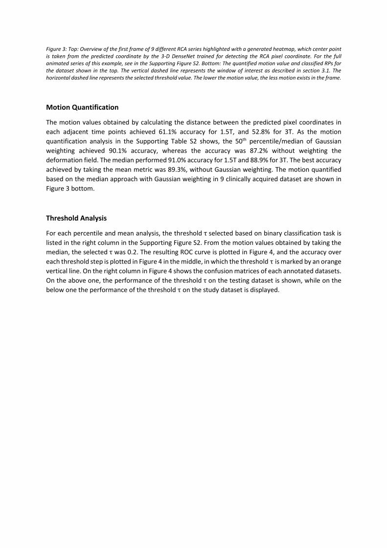
Figure 3: Top: Overview of the first frame of 9 different RCA series highlighted with a generated heatmap, which center point is taken from the predicted coordinate by the 3-D DenseNet trained for detecting the RCA pixel coordinate. For the full animated series of this example, see in the Supporting Figure S2. Bottom: The quantified motion value and classified RPs for the dataset shown in the top. The vertical dashed line represents the window of interest as described in section 3.1. The horizontal dashed line represents the selected threshold value. The lower the motion value, the less motion exists in the frame.
Motion Quantification
The motion values obtained by calculating the distance between the predicted pixel coordinates in
each adjacent time points achieved 61.1% accuracy for 1.5T, and 52.8% for 3T. As the motion
quantification analysis in the Supporting Table S2 shows, the 50th percentile/median of Gaussian
weighting achieved 90.1% accuracy, whereas the accuracy was 87.2% without weighting the
deformation field. The median performed 91.0% accuracy for 1.5T and 88.9% for 3T. The best accuracy
achieved by taking the mean metric was 89.3%, without Gaussian weighting. The motion quantified
based on the median approach with Gaussian weighting in 9 clinically acquired dataset are shown in
Figure 3 bottom.
Threshold Analysis
For each percentile and mean analysis, the threshold τ selected based on binary classification task is
listed in the right column in the Supporting Figure S2. From the motion values obtained by taking the
median, the selected τ was 0.2. The resulting ROC curve is plotted in Figure 4, and the accuracy over
each threshold step is plotted in Figure 4 in the middle, in which the threshold τ is marked by an orange
vertical line. On the right column in Figure 4 shows the confusion matrices of each annotated datasets.
On the above one, the performance of the threshold τ on the testing dataset is shown, while on the
below one the performance of the threshold τ on the study dataset is displayed.
Figure 4: Upper Left: the ROC curve from the threshold analysis is shown. Upper Right: the accuracy plot over the threshold values is shown. The best performed threshold value, 0.2 is marked in orange vertical line. Below Left: the confusion matrix showing the performance of binary classification task by taking the best threshold value on testing datasets. Below Right: the confusion matrix showing the performance by taking the best threshold value on study datasets. In each measure, the counts and rate in percentage are listed.
1.5T N = 22 0.20 93.4 90.1 96.8 3T N = 80 0.20 92.6 90.7 94.5 1.5T & 3T N = 102 0.20 92.7 90.5 95.0
Table 2: The results of the system on the study datasets are listed. In the first row, the difference between the start and end RP and expert annotations are shown. In the middle row, the difference of start and end systolic and diastolic RPs are shown in frame. In the last row, the accuracy, sensitive and specificity are listed with the optimally defined threshold.
The detailed results about the performance of the predicted systolic and diastolic RP on the study
datasets are listed in Table 2. The Bland-Altmann plots showing the performance of start and end
detected time point for each systolic and diastolic RP is shown in Figure 5.
𝑀𝐴𝐸𝑠𝑡𝑎𝑟𝑡,𝑒𝑛𝑑 𝑤𝑖𝑛𝑑𝑜𝑤/𝑓𝑟𝑎𝑚𝑒𝑠𝑦𝑠 and 𝑀𝐴𝐸𝑠𝑡𝑎𝑟𝑡,𝑒𝑛𝑑 𝑤𝑖𝑛𝑑𝑜𝑤/𝑓𝑟𝑎𝑚𝑒𝑑𝑖𝑎
for 1.5T datasets was 11.8 ± 16.5 ms
(0.38 ± 0.53 frame) and 14.2 ± 18.9 ms (0.48 ± 0.63 frame) for 3T datasets. By using the selected τ, the
proposed system resulted in 93.4% accuracy, sensitivity at 90.1% and specificity 96.8% for 1.5T and
92.6%, 90.7% and 94.5% for 3T datasets.
𝑀𝐴𝐸𝑠𝑡𝑎𝑟𝑡,𝑒𝑛𝑑 𝑤𝑖𝑛𝑑𝑜𝑤/𝑓𝑟𝑎𝑚𝑒𝑠𝑦𝑠 and 𝑀𝐴𝐸𝑠𝑡𝑎𝑟𝑡,𝑒𝑛𝑑 𝑤𝑖𝑛𝑑𝑜𝑤/𝑓𝑟𝑎𝑚𝑒𝑑𝑖𝑎
was 13.6 ± 18.6 ms (0.46 ± 0.62
frame) when using the datasets independent from field strength for analysis. The accuracy, sensitivity
and specificity achieved by the defined absolute τ , < 0.2, was 92.7%, 90.5% and 95.0%. The
automatically classified RPs resulted in a mean max error of ~30 ms, meaning that it deviates by roughly
one frame.
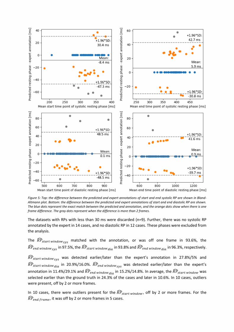
Figure 5: Top: the difference between the predicted and expert annotations of start and end systolic RP are shown in Bland-Altmann plot. Bottom: the difference between the predicted and expert annotations of start and end diastolic RP are shown. The blue dots represent the exact match between the predicted and annotation, and the orange dots show when there is one frame difference. The gray dots represent when the difference is more than 2 frames.
The datasets with RPs with less than 30 ms were discarded (n=9). Further, there was no systolic RP
annotated by the expert in 14 cases, and no diastolic RP in 12 cases. These phases were excluded from
the analysis.
The 𝑅�̂�𝑠𝑡𝑎𝑟𝑡 𝑤𝑖𝑛𝑑𝑜𝑤𝑠𝑦𝑠 matched with the annotation, or was off one frame in 93.6%, the
𝑅�̂�𝑒𝑛𝑑 𝑤𝑖𝑛𝑑𝑜𝑤𝑠𝑦𝑠 in 97.5%, the 𝑅�̂�𝑠𝑡𝑎𝑟𝑡 𝑤𝑖𝑛𝑑𝑜𝑤𝑑𝑖𝑎
in 93.8% and 𝑅�̂�𝑒𝑛𝑑 𝑤𝑖𝑛𝑑𝑜𝑤𝑑𝑖𝑎 in 96.3%, respectively.
𝑅�̂�𝑠𝑡𝑎𝑟𝑡 𝑤𝑖𝑛𝑑𝑜𝑤𝑠𝑦𝑠 was detected earlier/later than the expert’s annotation in 27.8%/5% and
𝑅�̂�𝑠𝑡𝑎𝑟𝑡 𝑤𝑖𝑛𝑑𝑜𝑤𝑑𝑖𝑎 in 20.9%/16.0%. 𝑅�̂�𝑒𝑛𝑑 𝑤𝑖𝑛𝑑𝑜𝑤𝑠𝑦𝑠
was detected earlier/later than the expert’s
annotation in 11.4%/29.1% and 𝑅�̂�𝑒𝑛𝑑 𝑤𝑖𝑛𝑑𝑜𝑤𝑑𝑖𝑎 in 15.2%/14.8%. In average, the 𝑅�̂�𝑠𝑡𝑎𝑟𝑡 𝑤𝑖𝑛𝑑𝑜𝑤 was
selected earlier than the ground truth in 24.3% of the cases and later in 10.6%. In 10 cases, outliers
were present, off by 2 or more frames.
In 10 cases, there were outliers present for the 𝑅�̂�𝑠𝑡𝑎𝑟𝑡 𝑤𝑖𝑛𝑑𝑜𝑤 , off by 2 or more frames. For the
𝑅�̂�𝑒𝑛𝑑 𝑓𝑟𝑎𝑚𝑒, it was off by 2 or more frames in 5 cases.
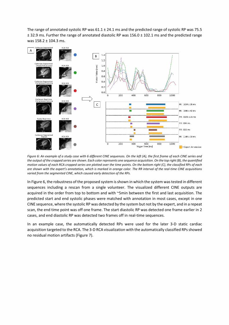
The range of annotated systolic RP was 61.1 ± 24.1 ms and the predicted range of systolic RP was 75.5
± 32.9 ms. Further the range of annotated diastolic RP was 156.0 ± 102.1 ms and the predicted range
was 158.2 ± 104.3 ms.
Figure 6: An example of a study case with 6 different CINE sequences. On the left (A), the first frame of each CINE series and the output of the cropped series are shown. Each color represents one sequence acquisition. On the top right (B), the quantified motion values of each RCA cropped series are plotted over the time points. On the bottom right (C), the classified RPs of each are shown with the expert’s annotation, which is marked in orange color. The RR interval of the real-time CINE acquisitions varied from the segmented CINE, which caused early detection of the RPs.
In Figure 6, the robustness of the proposed system is shown in which the system was tested in different
sequences including a rescan from a single volunteer. The visualized different CINE outputs are
acquired in the order from top to bottom and with ~5min between the first and last acquisition. The
predicted start and end systolic phases were matched with annotation in most cases, except in one
CINE sequence, where the systolic RP was detected by the system but not by the expert, and in a repeat
scan, the end time point was off one frame. The start diastolic RP was detected one frame earlier in 2
cases, and end diastolic RP was detected two frames off in real-time sequences.
In an example case, the automatically detected RPs were used for the later 3-D static cardiac
acquisition targeted to the RCA. The 3-D RCA visualization with the automatically classified RPs showed
no residual motion artifacts (Figure 7).
Figure 7: An example of a volunteer study illustrated with the main steps of the framework pipeline. The outputs are generated directly from the scanner after the proposed system was integrated online. The RCA localization series is the original CINE series with an RCA position marked by a cross. The ROI cropping generated the cropped series based on the RCA localization. From these cropped series, the motion is quantified, from which the RPs are determined. The series that represent the systolic and diastolic resting phase are generated as well. Here, the diastolic resting phase window (dark blue arrow) is applied for the static coronary imaging.
4. Discussion
The detection of the RCA ROI is successfully and robustly performed by the 3-D DenseNet on the testing
dataset and on the study cases. The 3-D based Conv networks leverage the spatial and temporal
information from the time-resolved input, rather than learning only spatial information per time point.
The size of the fixed ROI (50 x 50mm2) was sufficient in all cases for depicting the RCA at each time
point. Further, the network was robustly performed on different CINE sequences (Figure 6) which
allows the proposed system to be integrated into different clinical protocols.
In terms of quantifying motion values, the approach of taking the Euclidean distance from the
predicted RCA pixel coordinate over cardiac phases highly relies on the performance of the network,
furthermore, taking the pixel distance measurement for the displacement metric of the anatomy-of-
interest between the consecutive frames was not accurate as shown in Supporting Table S2. The
approaches deriving from the motion values by taking the deformation fields defined by the elastic
image registration show a clear advantage, from which the highest accuracy was the one using the
weighted deformation fields (see in Supporting Table S2). The approach with deformation fields is
clearly more robust to slight inaccuracies of localization results. The Gaussian weighting further
improves the performance of the system, as it allows to focus on the target-of-interest, and eliminates
the area which is not of interest, such as the blood flow in the atrium contained in the RCA ROI.
The metric for assessing the motion values from the weighted deformation fields was reasonably
chosen as 50th percentile by the accuracy analysis. The absolute threshold value is selected based on
AUC-ROC analysis, evaluated on the testing datasets from the different 1.5T, 3T scanners and CINE
sequences and no specific data selection, thus shows versatility in the results (Figure 4). The
classification of the RP by the absolute threshold value is possible due to the quantitative outputs of
the deformation field-based approach which enables the detection of the phases with minimal motion
by not limiting the RP window length, which can be either end-systolic or mid-diastolic or end-systolic
and mid-diastolic RPs.
In Figure 4, the quantified motion values of the clinically acquired dataset with different CINE
sequences and the corresponding predicted RPs were well matched with the expert’s annotation. As
shown in Table 2, the proposed framework performed robust in different field strengths as well.
Interestingly, in the dataset visualized in the center, there was no RP found by a medical expert, and
the proposed system was also able to classify the non-RP case demonstrating the advantage of the
system. In such cases, the system gives the user the possibility to take the quantified curve as a
reference and select the phase with minimum motion based on the motion curve.
Based on the Bland-Altmann plots (Figure 5), the systolic RP did not perform as well as the diastolic RP,
especially the classification of the start systolic RP was challenging. The predicted systolic RP window
was usually slightly longer than the experts’ annotations. However, the mean range difference was 15
ms, which is negligible since the temporal resolution of CINE series is ~30 ms.
As shown in Figure 7, the RCA was sharply visualized without severe residual motion artifacts that was
acquired during the automatically detected RPs.
Previous methods have shown the feasibility to detect the imaging acquisition window automatically
using the shim box volume positioning and cross-correlation calculation [21, 22]. However, these semi-
automated methods still require the careful positioning of the shim volume coverage. Further, the RP
detection is targeted to the whole heart instead of a specific anatomy of interest. These methods were
validated on healthy in vivo subjects on a single field strength.
Moreover, approaches based on the standard deviation of pixel intensity [24] or difference of gradient
magnitudes [42] were introduced, allowing the RP detection in real time. This method however
performs the RP detection globally based on the entire field-of-view, and the detected RPs are always
two RPs as the search is done by two local minima.
Several approaches have been proposed for the automated determination of targeted RP on regions
such as RCA [23, 25]. A template matching was performed for finding the area with the outer edge of
the cross-section of the coronary artery, however the template was defined based on randomly
selected five datasets [23]. In a more recent study, the regions were extracted from the high-speed
component within CINE series by the frequency domain analysis, however by doing so, the cardiac
anatomy structures can be disregarded. The authors stated that this method was validated on healthy
volunteers, and uncertain the performance on large dataset especially with high heart rates.
In [43], the deep learning-based RP detection network is built by combining the CNN and Long short-
term memory models taking the CINE series as input, and outputs the binary output which is either a
RP or not a RP. Therefore, this method is not quantitative and unclear which cardiac structure is
weighted, or whether the network tries to detect global RP.
5. Conclusions
To our knowledge, this proposed study is the first to present the fully automated localized RP detection
framework from a CINE series that was validated with a large dataset with multiple 1.5T and 3T
scanners acquired with different CINE protocols, such as with free-breathing or breath-held techniques.
We investigated the robustness and feasibility of the proposed system for fully automated systolic and
diastolic RP detection. The proposed system can improve the workflow efficiency, automation, and
standardization of the static cardiac imaging that broaden the applicability towards any static cardiac
imaging. The RP detection system can be applied in various applications, such as 2-D and 3-D LGE,
mapping, 3-D coronary imaging, or any other applications in which the information of RP of heart can
be useful.
Future work will focus on clinical validations, improving the accuracy of RP classification and
integration of automatic detection of other regions, such as the atria and ventricles.
Reference
[1] P. Kellman and A. E. Arai, "Cardiac imaging techniques for physicians: late enhancement,"
Journal of magnetic resonance imaging, vol. 36, p. 529–542, 2012.
[2] P. Kellman, A. E. Arai, E. R. McVeigh and A. H. Aletras, "Phase-sensitive inversion recovery for
detecting myocardial infarction using gadolinium-delayed hyperenhancement," Magnetic
Resonance in Medicine: An Official Journal of the International Society for Magnetic Resonance
in Medicine, vol. 47, p. 372–383, 2002.
[3] M. Akçakaya, H. Rayatzadeh, T. A. Basha, S. N. Hong, R. H. Chan, K. V. Kissinger, T. H. Hauser, M.
E. Josephson, W. J. Manning and R. Nezafat, "Accelerated late gadolinium enhancement cardiac
MR imaging with isotropic spatial resolution using compressed sensing: initial experience,"
Radiology, vol. 264, p. 691–699, 2012.
[4] T. A. Basha, M. Akcakaya, C. Liew, C. W. Tsao, F. N. Delling, G. Addae, L. Ngo, W. J. Manning and
R. Nezafat, "Clinical performance of high-resolution late gadolinium enhancement imaging with
compressed sensing," Journal of Magnetic Resonance Imaging, vol. 46, p. 1829–1838, 2017.
[5] P. Kellman and M. S. Hansen, "T1-mapping in the heart: accuracy and precision," Journal of
cardiovascular magnetic resonance, vol. 16, p. 1–20, 2014.
[6] D. R. Messroghli, J. C. Moon, V. M. Ferreira, L. Grosse-Wortmann, T. He, P. Kellman, J.
Mascherbauer, R. Nezafat, M. Salerno, E. B. Schelbert and others, "Clinical recommendations
for cardiovascular magnetic resonance mapping of T1, T2, T2* and extracellular volume: a
consensus statement by the Society for Cardiovascular Magnetic Resonance (SCMR) endorsed
by the European Association for Cardiovascular Imaging (EACVI)," Journal of Cardiovascular
Magnetic Resonance, vol. 19, p. 1–24, 2017.
[7] E. Aherne, K. Chow and J. Carr, "Cardiac T1 mapping: techniques and applications," Journal of
Magnetic Resonance Imaging, vol. 51, p. 1336–1356, 2020.
[8] C. Munoz, A. Bustin, R. Neji, K. P. Kunze, C. Forman, M. Schmidt, R. Hajhosseiny, P.-G. Masci, M.
Zeilinger, W. Wuest and others, "Motion-corrected 3D whole-heart water-fat high-resolution
late gadolinium enhancement cardiovascular magnetic resonance imaging," Journal of
Cardiovascular Magnetic Resonance, vol. 22, p. 1–13, 2020.
[9] G. Greil, A. A. Tandon, M. Silva Vieira and T. Hussain, "3D whole heart imaging for congenital
heart disease," Frontiers in pediatrics, vol. 5, p. 36, 2017.
[10] G. Cruz, D. Atkinson, M. Henningsson, R. M. Botnar and C. Prieto, "Highly efficient nonrigid
motion-corrected 3D whole-heart coronary vessel wall imaging," Magnetic resonance in
medicine, vol. 77, p. 1894–1908, 2017.
[11] C. Forman, D. Piccini, R. Grimm, J. Hutter, J. Hornegger and M. O. Zenge, "Reduction of
Respiratory Motion Artifacts for Free-Breathing Whole-Heart Coronary MRA by Weighted
Iterative Reconstruction," Magnetic Resonance in Medicine, p. 1–11, 2014.
[12] C. M. Kramer, J. Barkhausen, C. Bucciarelli-Ducci, S. D. Flamm, R. J. Kim and E. Nagel,
"Standardized cardiovascular magnetic resonance imaging (CMR) protocols: 2020 update,"
Journal of Cardiovascular Magnetic Resonance, vol. 22, p. 1–18, 2020.
[13] H. Isma’eel, Y. S. Hamirani, R. Mehrinfar, S. Mao, N. Ahmadi, V. Larijani, S. Nair and M. J. Budoff,
"Optimal phase for coronary interpretations and correlation of ejection fraction using late-
diastole and end-diastole imaging in cardiac computed tomography angiography: implications
for prospective triggering," The international journal of cardiovascular imaging, vol. 25, p. 739–
749, 2009.
[14] C. M. Kramer, J. Barkhausen, S. D. Flamm, R. J. Kim and E. Nagel, "Society for Cardiovascular
Magnetic Resonance Board of trustees task force on standardized P. Standardized
Supporting Figure S1: A box plot showing the performance of the 122-layer 3-D DenseNet in each time point is illustrated.
Supporting Figure S2: Full animated time series of a part of the study dataset shown in Fig. 2 are visualized (n=9).
Supporting Table S1: The extended 3-D DenseNet built for the RCA detection. Each Conv consists of the successively executed layers of 3-D batch normalization, rectified linear unit activation function and 3-D convolutions. For the RCA detection, the 3-D DenseNet with the total number of 122 convolutional layers are built as follows: d=32, h,w=224 and c1,2,3,4 = {6,12,24,16}.
Supporting Table S2: The analysis of motion quantification. Two approaches by using the Gaussian weighting of the magnitude of the deformation fields, or without any weighting have been compared for varying the percentile and taking the mean value.
Supporting Information
Supporting Figure S1: A box plot showing the performance of the 122-layer 3-D DenseNet in each time