Automated Mapping of Convective Clouds (AMCC) Thermodynamical, Microphysical, and CCN Properties from SNPP/VIIRS Satellite Data ZHIGUO YUE, a,b DANIEL ROSENFELD, c GUIHUA LIU, a JIN DAI, a XING YU, a YANNIAN ZHU, a EYAL HASHIMSHONI, c XIAOHONG XU, a YING HUI, a AND OLIVER LAUER d a Meteorological Institute of Shaanxi Province, Xi’an, China b Office of Weather Modification of Shaanxi Province, Xi’an, China c Institute of Earth Sciences, Hebrew University of Jerusalem, Jerusalem, Israel d Multiphase Chemistry Department, Max Planck Institute for Chemistry, Mainz, Germany (Manuscript received 7 June 2018, in final form 19 January 2019) ABSTRACT The advent of the Visible Infrared Imager Radiometer Suite (VIIRS) on board the Suomi NPP (SNPP) satellite made it possible to retrieve a new class of convective cloud properties and the aerosols that they ingest. An automated mapping system of retrieval of some properties of convective cloud fields over large areas at the scale of satellite coverage was developed and is presented here. The system is named Automated Mapping of Convective Clouds (AMCC). The input is level-1 VIIRS data and meteorological gridded data. AMCC identifies the cloudy pixels of convective elements; retrieves for each pixel its temperature T and cloud drop effective radius r e ; calculates cloud-base temperature T b based on the warmest cloudy pixels; calculates cloud-base height H b and pressure P b based on T b and meteorological data; calculates cloud-base updraft W b based on H b ; calculates cloud-base adiabatic cloud drop concentrations N d,a based on the T–r e relationship, T b , and P b ; calculates cloud-base maximum vapor supersaturation S based on N d,a and W b ; and defines N d,a /1.3 as the cloud condensation nuclei (CCN) concentration N CCN at that S. The results are gridded 36 km 3 36 km data points at nadir, which are sufficiently large to capture the properties of a field of con- vective clouds and also sufficiently small to capture aerosol and dynamic perturbations at this scale, such as urban and land-use features. The results of AMCC are instrumental in observing spatial covariability in clouds and CCN properties and for obtaining insights from such observations for natural and man-made causes. AMCC-generated maps are also useful for applications from numerical weather forecasting to climate models. 1. Introduction Satellite retrievals are the only practical way of ob- serving clouds and aerosol properties on regional and global scales. Recently Rosenfeld et al. (2016) was able to use such satellite retrievals to provide estimation of cloud condensation nuclei (CCN) concentration N CCN from satellite measurements. In this study we take the next step and present a method for application of the CCN retrievals for mapping large areas. The main part of this paper presents the method of CCN mapping. The introduction prepares the background by reviewing the physical basis for CCN retrieval. Aerosols affect clouds mainly by their CCN activity, which influences cloud drop number concentrations and albedo, which in turn is followed by a cascade of ad- justment processes that can either buffer or amplify the primary effect on cloud radiative properties (Stevens and Feingold 2009). Therefore, much of the science of atmospheric chemistry and aerosols has been devoted to ways by which aerosol size and composition determine their CCN and ice nucleating particle activity (Andreae and Rosenfeld 2008). Satellite observation retrievals are the only practical way to quantify the effective radiative forcing by aerosol cloud interactions at a global scale. Aerosol optical-depth retrieval near clouds is plagued by artifacts (Várnai and Marshak 2009) and ambiguity (Quaas et al. 2010), and it is only crudely related to CCN (Andreae 2009). Even if AOD could be retrieved accurately, it would likely be poorly correlated with the actual CCN that affects clouds (Stier 2016). Furthermore, aerosol effects on cloud composition are entangled with meteorological conditions, mainly as manifested by updraft Corresponding author: Daniel Rosenfeld, daniel.rosenfeld@ mail.huji.ac.il APRIL 2019 YUE ET AL. 887 DOI: 10.1175/JAMC-D-18-0144.1 Ó 2019 American Meteorological Society. For information regarding reuse of this content and general copyright information, consult the AMS Copyright Policy (www.ametsoc.org/PUBSReuseLicenses). Unauthenticated | Downloaded 03/24/22 11:42 AM UTC
Transcript
Automated Mapping of Convective Clouds (AMCC) Thermodynamical, Microphysical,and CCN Properties from SNPP/VIIRS Satellite Data
ZHIGUO YUE,a,b DANIEL ROSENFELD,c GUIHUA LIU,a JIN DAI,a XING YU,a YANNIAN ZHU,a
EYAL HASHIMSHONI,c XIAOHONG XU,a YING HUI,a AND OLIVER LAUERd
aMeteorological Institute of Shaanxi Province, Xi’an, ChinabOffice of Weather Modification of Shaanxi Province, Xi’an, China
c Institute of Earth Sciences, Hebrew University of Jerusalem, Jerusalem, IsraeldMultiphase Chemistry Department, Max Planck Institute for Chemistry, Mainz, Germany
(Manuscript received 7 June 2018, in final form 19 January 2019)
ABSTRACT
The advent of the Visible Infrared Imager Radiometer Suite (VIIRS) on board the Suomi NPP (SNPP)
satellite made it possible to retrieve a new class of convective cloud properties and the aerosols that they
ingest. An automated mapping system of retrieval of some properties of convective cloud fields over large
areas at the scale of satellite coverage was developed and is presented here. The system is named Automated
Mapping of Convective Clouds (AMCC). The input is level-1 VIIRS data and meteorological gridded data.
AMCC identifies the cloudy pixels of convective elements; retrieves for each pixel its temperature T and
cloud drop effective radius re; calculates cloud-base temperature Tb based on the warmest cloudy pixels;
calculates cloud-base height Hb and pressure Pb based on Tb and meteorological data; calculates cloud-base
updraft Wb based on Hb; calculates cloud-base adiabatic cloud drop concentrations Nd,a based on the T–rerelationship, Tb, and Pb; calculates cloud-base maximum vapor supersaturation S based on Nd,a andWb; and
definesNd,a/1.3 as the cloud condensation nuclei (CCN) concentrationNCCN at that S. The results are gridded
36 km 3 36 km data points at nadir, which are sufficiently large to capture the properties of a field of con-
vective clouds and also sufficiently small to capture aerosol and dynamic perturbations at this scale, such as
urban and land-use features. The results of AMCC are instrumental in observing spatial covariability in
clouds and CCN properties and for obtaining insights from such observations for natural and man-made
causes. AMCC-generated maps are also useful for applications from numerical weather forecasting to
climate models.
1. Introduction
Satellite retrievals are the only practical way of ob-
serving clouds and aerosol properties on regional and
global scales. Recently Rosenfeld et al. (2016) was able
to use such satellite retrievals to provide estimation of
from satellite measurements. In this study we take the
next step and present a method for application of the
CCN retrievals for mapping large areas. The main part
of this paper presents the method of CCNmapping. The
introduction prepares the background by reviewing the
physical basis for CCN retrieval.
Aerosols affect clouds mainly by their CCN activity,
which influences cloud drop number concentrations and
albedo, which in turn is followed by a cascade of ad-
justment processes that can either buffer or amplify the
primary effect on cloud radiative properties (Stevens
and Feingold 2009). Therefore, much of the science of
atmospheric chemistry and aerosols has been devoted to
ways by which aerosol size and composition determine
their CCN and ice nucleating particle activity (Andreae
and Rosenfeld 2008). Satellite observation retrievals are
the only practical way to quantify the effective radiative
forcing by aerosol cloud interactions at a global scale.
Aerosol optical-depth retrieval near clouds is plagued
by artifacts (Várnai and Marshak 2009) and ambiguity
(Quaas et al. 2010), and it is only crudely related to
CCN (Andreae 2009). Even if AOD could be retrieved
accurately, it would likely be poorly correlated with the
actual CCN that affects clouds (Stier 2016). Furthermore,
aerosol effects on cloud composition are entangled with
meteorological conditions, mainly as manifested by updraftCorresponding author: Daniel Rosenfeld, daniel.rosenfeld@
mail.huji.ac.il
APRIL 2019 YUE ET AL . 887
DOI: 10.1175/JAMC-D-18-0144.1
� 2019 American Meteorological Society. For information regarding reuse of this content and general copyright information, consult the AMS CopyrightPolicy (www.ametsoc.org/PUBSReuseLicenses).
Unauthenticated | Downloaded 03/24/22 11:42 AM UTC
speeds. Without simultaneously retrieving both cloud
active aerosols and cloud-base updrafts Wb, it is im-
possible to disentangle and extract the net aerosol ef-
fects. To make matters worse, the ability to retrieveWb
via satellite has been nonexistent until our very recent
studies (Zheng and Rosenfeld 2015; Zheng et al.
2015, 2016).
Cloud pixel temperature–cloud drop effective radius,
or T–re, relationships were first constructed by Rosenfeld
and Lensky (1998) for inferring the microstructure and
precipitation forming processes of convective clouds.
The T–re relationships are used to retrieve glaciation
temperature Tg of convective clouds (Rosenfeld et al.
2011; Yuan et al. 2010) and the depth of precipitation
initiation. This depthD14 is the height within the cloud
at which the retrieved re reaches 14mm—the point
above which the probability of precipitation increases
(Freud et al. 2008; Freud and Rosenfeld 2012;
Rosenfeld 1999; Rosenfeld and Gutman 1994; Zhu
et al. 2015). The observed brightness temperature at
the top of this layer is T14. The depth of precipitation
initiation D14 may also be related to convective storm
severity (Rosenfeld et al. 2008a). As a result of the
previously mentioned studies, it is now possible to use
VIIRS for retrieving a set of convective cloud products
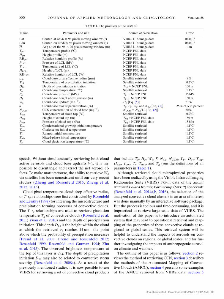
that include Tb, Hb, Wb, S, Nd,a, NCCN, T14, D14, Ttop,
Htop, Tcon, Tr, Tmix, and Tg (see the definitions of all
parameters in Table 1).
Although retrieved cloud microphysical properties
have been realized by using theVisible Infrared Imaging
Radiometer Suite (VIIRS) 375-m data of the Suomi
National Polar-Orbiting Partnership (SNPP) spacecraft
(Rosenfeld et al. 2014a,b, 2016), the selection of the
analyzed convective cloud clusters in an area of interest
was done manually by an interactive software package.
But the process is tedious and time-consuming, and it is
impractical to retrieve large-scale data of VIIRS. The
motivation of this paper is to introduce an automated
system that may lead to operational retrieval and map-
ping of the properties of these convective clouds at re-
gional to global scales. This retrieval system will be
helpful to understand the impacts of aerosols on con-
vective clouds on regional or global scales, and for fur-
ther investigating the impacts of anthropogenic aerosol
on climate and weather.
The outline of this paper is as follows: Section 2 re-
views the method of retrieving CCN, section 3 describes
the methods of the Automated Mapping of Convec-
tive Clouds (AMCC), section 4 presents some examples
of the AMCC retrieval from VIIRS data, section 5
TABLE 1. The products of the AMCC.
Name Parameter and unit Source of calculation Error
Lat Center lat of 96 3 96 pixels moving window (8) VIIRS L1b image data 0.00018Lon Center lon of 96 3 96 pixels moving window (8) VIIRS L1b image data 0.00018H Avg alt of the 96 3 96 pixels moving window (m) VIIRS L1b image data 1m
Tprf Temperature profile (8C) NCEP FNL data
Hprf Height profile (m) NCEP FNL data
RHprf Relative humidity profile (%) NCEP FNL data
PLCL Pressure of LCL (hPa) NCEP FNL data
TLCL Temperature of LCL (8C) NCEP FNL data
HLCL Height of LCL (m) NCEP FNL data
RHLCL Relative humidity of LCL (%) NCEP FNL data
re,b Cloud-base drop effective radius (mm) Satellite retrieval 8%
T14 Temperature of precipitation initiation Satellite retrieval 0.28CD14 Depth of precipitation initiation T14 1 NCEP FNL 150m
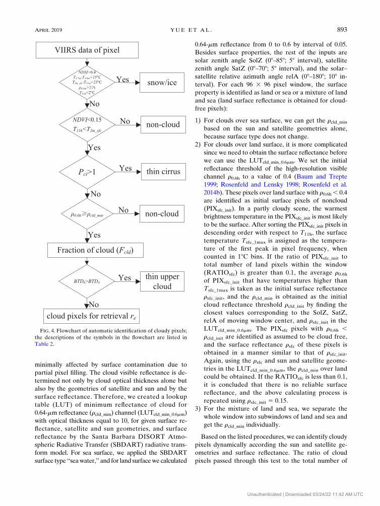
terval). For each 96 3 96 pixel window, the surface
property is identified as land or sea or a mixture of land
and sea (land surface reflectance is obtained for cloud-
free pixels):
1) For clouds over sea surface, we can get the rcld_min
based on the sun and satellite geometries alone,
because surface type does not change.
2) For clouds over land surface, it is more complicated
since we need to obtain the surface reflectance before
we can use the LUTcld_min_0.6mm. We set the initial
reflectance threshold of the high-resolution visible
channel r0.6h to a value of 0.4 (Baum and Trepte
1999; Rosenfeld and Lensky 1998; Rosenfeld et al.
2014b). These pixels over land surface with r0.6h, 0.4
are identified as initial surface pixels of noncloud
(PIXsfc_init). In a partly cloudy scene, the warmest
brightness temperature in the PIXsfc_init is most likely
to be the surface. After sorting the PIXsfc_init pixels in
descending order with respect to T11h, the surface
temperature Tsfc_1max is assigned as the tempera-
ture of the first peak in pixel frequency, when
counted in 18C bins. If the ratio of PIXsfc_init to
total number of land pixels within the window
(RATIOsfc) is greater than 0.1, the average r0.6hof PIXsfc_init that have temperatures higher than
Tsfc_1max is taken as the initial surface reflectance
rsfc_init, and the rcld_min is obtained as the initial
cloud reflectance threshold rcld_init by finding the
closest values corresponding to the SolZ, SatZ,
relA of moving window center, and rsfc_init in the
LUTcld_min_0.6mm. The PIXsfc pixels with r0.6h ,rcld_init are identified as assumed to be cloud free,
and the surface reflectance rsfc of these pixels is
obtained in a manner similar to that of rsfc_init.
Again, using the rsfc and sun and satellite geome-
tries in the LUTcld_min_0.6mm, the rcld_min over land
could be obtained. If the RATIOsfc is less than 0.1,
it is concluded that there is no reliable surface
reflectance, and the above calculating process is
repeated using rsfc_init 5 0.15.
3) For the mixture of land and sea, we separate the
whole window into subwindows of land and sea and
get the rcld_min individually.
Based on the listed procedures, we can identify cloudy
pixels dynamically according the sun and satellite ge-
ometries and surface reflectance. The ratio of cloud
pixels passed through this test to the total number of
FIG. 4. Flowchart of automatic identification of cloudy pixels;
the descriptions of the symbols in the flowchart are listed in
Table 2.
APRIL 2019 YUE ET AL . 893
Unauthenticated | Downloaded 03/24/22 11:42 AM UTC
pixels of the moving window is defined as the fraction of
cloud Fcld.
5) REJECTION OF MULTILAYER CLOUD PIXELS
Because brightness temperature of the colder cloud
pixels is affected by less water vapor absorption, the
difference of brightness temperature (BTD) of a thick
cloud should decrease with decreasing temperature.
However, when a thin cloud overlaps another clouds,
the brightness temperature and reflectance of these
cloud pixels are disturbed, and the BTD will be in-
creased (Inoue 1987). It is necessary to exclude those
cloud pixels that are optically thin or newly formed
water clouds over lower clouds because they lead to an
overestimate the BTD. Traditionally, BTD between 11
and 12mmwas used to reject such types of clouds (Inoue
1985). Rosenfeld et al. (2014b) have developed a
method to obtain BTD of 375-m resolution (BTDh)
because of the fact that 12.0mm is not available sepa-
rately at 375-m resolution of VIIRS. For a given T11h,
pixels that have passed through cloud mask of sections
3c(2) and 3c(3) (PIXcld) in this moving window are
sorted from small to large BTDh, and the BTDh of 25th-
percentile pixel number is marked as BTD4 for thisT11h.
TABLE 2. The symbols used in this paper, with their descriptions and units.
Symbol Parameter and unit Source of calculation Error
re Cloud drop effective radius (mm) Satellite retrieval 8%
Wb Cloud-base updraft (m s21) Hb [Eq. (5)] 27%
T Cloud pixel temperature (8C) Satellite retrieval 0.28CT14 Temperature of precipitation initiation (8C) Satellite retrieval 0.28CD14 Depth of precipitation initiation T14 1 NCEP FNL 150m
Tg Cloud glaciation temperature (8C) Satellite retrieval
NDSI Normalized difference snow index NDSI5 (r0.56m2 r1.6m)/(r0.56m1 r1.6m)
T3.7m 3.7-mm brightness temperature of 750-m resolution (8C) VIIRS L1b image data 0.4%
T4.0m 4.05-mm brightness temperature of 750-m resolution (8C) VIIRS L1b image data 0.4%
T8.6m 8.55-mm brightness temperature of 750-m resolution (8C) VIIRS L1b image data 0.4%
T11m 10.76-mm brightness temperature of 750-m resolution (8C) VIIRS L1b image data 0.4%
T11h 11.45-mm brightness temperature of 375-m resolution (8C) VIIRS L1b image data 0.4%
T12m 12.0-mm brightness temperature of 750-m resolution (8C) VIIRS L1b image data 0.4%
T2m_sfc 2-m temperature above the surface (8C) NCEP FNL
DT11h Pixel homogeneity Eq. (7)
BTDh Difference of brightness temperature of cloudy pixels for high
resolution (375m)
Recalibrated T11h 2 T11m (Rosenfeld
et al. 2014b)
BTD4 The BTDh of 25th-percentile pixels no. of moving window VIIRS L1b image data
CVI Convection index of moving window
Fcld Fraction of cloud pixels of moving window
Fre The fraction of re . 0 pixels of moving window
re Mean re of moving window (mm)
894 JOURNAL OF APPL IED METEOROLOGY AND CL IMATOLOGY VOLUME 58
Unauthenticated | Downloaded 03/24/22 11:42 AM UTC
The BTD4 values from the highest to the lowest T11h of
PIXcld are calculated. If BTD4 of a given T11h increases
with decreasing T11h, it is replaced by the monotonically
decreasing or invariant BTD4, which is obtained by the
linear interpolation of the nearest BTD4 with decreasing
T11h. Then, themonotonic reduction is enforced for BTD4
of PIXcld with decreasing T11h because only optically thin
upper clouds can increase BTD4 with decreasing T11h.
BTD4 dynamically obtained for each T11h of PIXcld in
each moving window is used as a criterion for identifying
overlapped thin upper clouds. If BTDh of a cloud pixel is
greater than BTD4 corresponding to its T11h, it will be
masked as overlapped thin upper clouds and rejected.
d. re retrieval
The 3.74-mm reflectance r3.7h is used to retrieve re from a
lookup table (LUTre; Kaufman and Nakajima 1993;
Rosenfeld and Lensky 1998) for the pixels identified as
cloudy using the cloud screening described above. The
LUTre is established for an effective radius of the water
cloud drop for given re, r3.7h, SolZ, SatZ, and relA
(Rosenfeld and Lensky 1998; Rosenfeld et al. 2014b). The
r3.7h of larger cloud particles decreases to near the channel
noise level, so the maximum size of re retrieved by this
method is 40mm. Note that, because the liquid phase re is
from 1 to 40mm in LUTre, the allowable retrieval solution
space for liquid clouds is limited to 1–40mm. The percent-
age of re . 0 pixels in the moving window Fre is obtained.
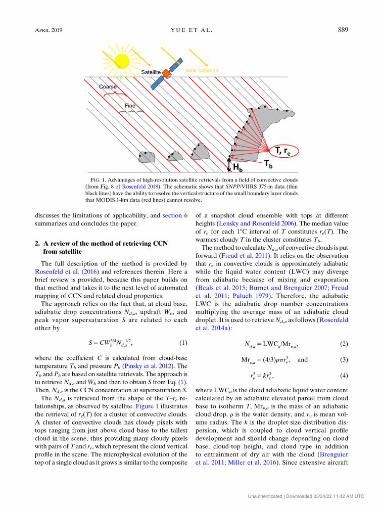
e. Convective clouds detection
The clouds addressed in this study are generated by
convection that is propelled by surface heating and
consist of convective clouds with flat base at the lifting
condensation level (LCL), as illustrated in Fig. 1.
Therefore, early-afternoon satellite overpasses are best
suited for observing such convective clouds over land.
Boundary layer convective clouds over ocean are much
less affected by the diurnal cycle.
Aircraft measurements of vertical microphysical pro-
files of such convective clouds show that cloud droplet reincreases monotonically from cloud base to top in de-
veloping convective clouds (Andreae et al. 2004; Konwar
et al. 2012; Prabha et al. 2011; Rosenfeld and Lensky
1998; Rosenfeld and Woodley 2000; Rosenfeld et al.
2006; Braga et al. 2017), and cloud-top re in different
stages of a vertically growing convective clouds cluster
are similar to the re of different heights within a single
convective cloud. This relationship of increasing re with
height is often ambiguous for nonconvective clouds,
however.As the temperature decreases with the increase
of height, the positive correlation between re and cloud-
top height is characterized by a corresponding negative
correlation between re and temperature. Thus, the T–re
relationships can be used to separate a mixture of layer
and convective clouds (Lensky and Rosenfeld 1997) and
applied to detection of convective clouds. The following
four steps are used to distinguish the convective and
nonconvective clouds in each moving window.
1) The analysis is done on a small runningwindow of 25325 5 625 pixels in a moving window, centered at the
tested cloudy pixel. The re and T values of an inner
small running window are sorted from high to low by
temperature. The correlation coefficient between the
sorted T and re is calculated as the relation of convec-
tion Rcv. A negative Rcv means increasing re with
decreasing T, which characterizes a convective cloud.
2) The Rcv of each cloud pixel in the moving window is
calculated.
3) The average value of Rcv of all cloud pixels in the
moving window is defined as the convection index
(CVI). If CVI. 0, the cloud in this moving window is
not a convective cloud.
4) The T–re profile of retrieval CCN is required to start
from cloud base. If most pixels of the moving window
are cloudy, there is a risk of insufficient documenta-
tion of the lower parts of the clouds. On the other
extreme, the T–re profile cannot be established with
too few cloud pixels with re. Aircraft measurements
show that the cloud base re is generally in the range of
1–8mm and that formation of precipitation-sized
drops occurs when re . 13mm (Braga et al. 2017;
Rosenfeld et al. 2006, 2008b). Too large of a mean re,
or re, indicates glaciated clouds. Therefore, a cloud is
identified as water convective cloud when CVI , 0
and Fcld , 95% and Fre . 0.4% and re , 35mm.
f. The retrieval of convective clouds basetemperature (Tb)
The cloud base is taken as the warmest cloudy pixel in a
moving window of convective clouds having different ex-
tent of vertical development above their base. Cloud base
is assumed to be at constant heights for convective clouds
over awell-mixed boundary layer.Under these conditions,
the warmest cloudy pixel can approximate Tb. Here the
algorithm of Zhu et al. (2014) is used for retrieving Tb.
It is based on pixel homogeneity DT11h, which is the
pixel homogeneity parameter of the 11.45-mm bright-
ness temperature T11h at 375-m resolution. The DT11h
was defined as (Rosenfeld et al. 2014b)
DT11h
51
4�4
i51
jT11hi
2T11h
j , (7)
where T11h is the brightness temperature average of
four pixels in the 375-m-resolution channel that reside
APRIL 2019 YUE ET AL . 895
Unauthenticated | Downloaded 03/24/22 11:42 AM UTC
within one 750-m-resolution pixel and T11hi is the T11h
of each these four points, respectively. If DT11h is
greater than the given threshold (DT11h_threshold5 18C),it is considering to be a mixed pixel by cloud and sur-
face. All of the pixels within the moving window are
sorted by their T11h. The warmest T11h for which a
percentile DT11h (P_DT11h) of DT11h ,DT11h_threshold is
considered to be theTb. A value ofP_DT11h5 30%was
found to be optimal (Zhu et al. 2014). This method was
validated against a combination of ceilometer and
sounding with Tb RMS error of 1.18C over the SGP site.
An error of 61.18C in Tb propagates to an ;5% error in
the retrieved Nd,a (Rosenfeld et al. 2016).
g. Identification the adiabatic re and retrieval CCN
Because the calculation of CCN is based on the
adiabatic assumption of convective clouds, it is very
important to identify the nearly adiabatic part from the
T–re profile of convective clouds. To avoid the in-
authentic re of nearby cloud base that is due to surface
contamination, the warmest temperature level is skip-
ped. If re . 15mm at their lowest 500m or re . 20mm
in the T–re profile, an underestimate of CCN would
otherwise result because of active cloud droplet coa-
lescence or heavily precipitation. Therefore, the ap-
proximate adiabatic part of convective clouds will be
searched from Tb 2 18C with re , 15mm at the lowest
500m to the T with the first re 5 20mm (T20mm). LWCa
should increase monotonically with decreasing tem-
perature or increasing droplet mass in an ideal adia-
batic condition. Therefore, the slope of linear best fit is
calculated between LWCa and Mry,a from Tb 2 18C to
each T with T, T20mm, and the fit is forced to Mry,a 5 0
at LWCa 5 0. The maximum slope is the end of adia-
batic process and the respectiveNd,a [Eq. (2)]. Because
of the mean deviation from the extreme inhomoge-
neous mixing assumption, the NCCN is equal to Nd,a
divided by 1.3 (Freud et al. 2011; Rosenfeld et al.
2014a, 2016).
h. Quality control and display
A postprocessing procedure is to eliminate the
convective clouds that are not suitable for retrieval
boundary layer CCN. These cloud bases are elevated
and, consequently, not coupled to the surface. The
filtering of such elevated clouds is made mainly by
analyzing the spatial distribution of Tb. Each Tb is
compared with all Tb in the box area of 28 3 28 latitudeand longitude that is centered on itself. The median
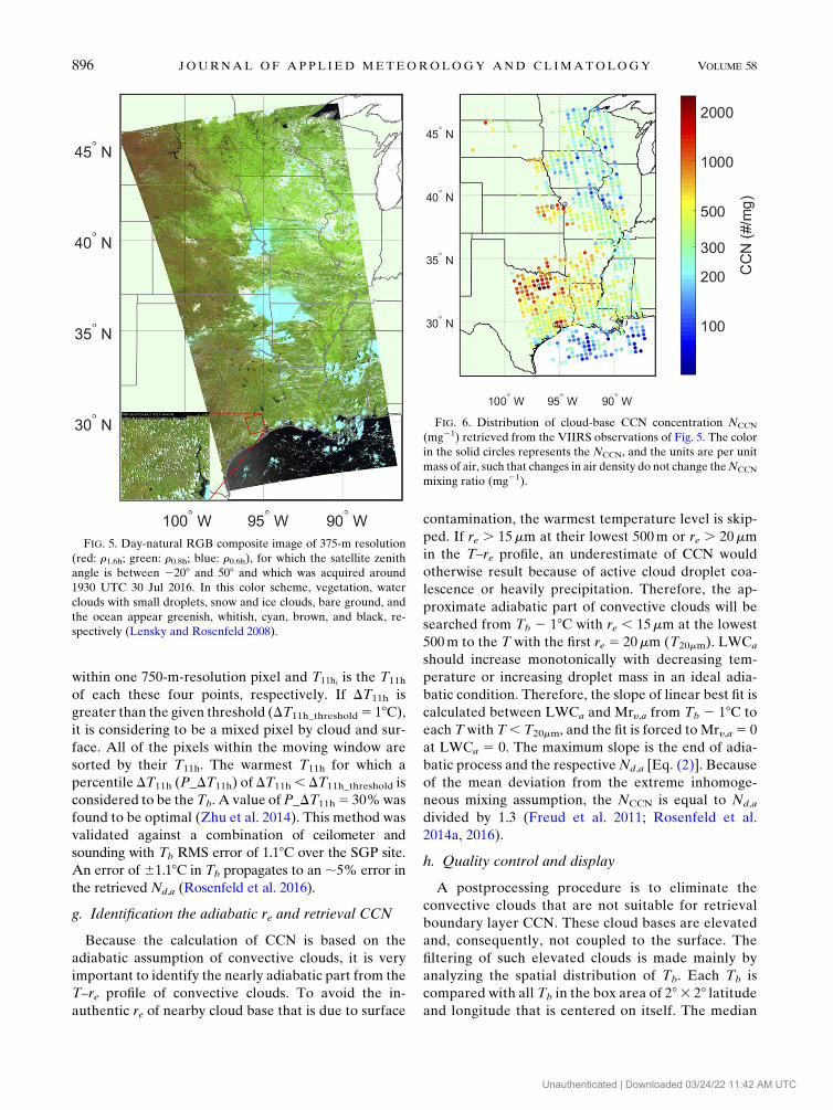
FIG. 5. Day-natural RGB composite image of 375-m resolution
(red: r1.6h; green: r0.8h; blue: r0.6h), for which the satellite zenith
angle is between 2208 and 508 and which was acquired around
1930 UTC 30 Jul 2016. In this color scheme, vegetation, water
clouds with small droplets, snow and ice clouds, bare ground, and
the ocean appear greenish, whitish, cyan, brown, and black, re-
spectively (Lensky and Rosenfeld 2008).
FIG. 6. Distribution of cloud-base CCN concentration NCCN
(mg21) retrieved from the VIIRS observations of Fig. 5. The color
in the solid circles represents the NCCN, and the units are per unit
mass of air, such that changes in air density do not change theNCCN
mixing ratio (mg21).
896 JOURNAL OF APPL IED METEOROLOGY AND CL IMATOLOGY VOLUME 58
Unauthenticated | Downloaded 03/24/22 11:42 AM UTC
of Tb, or Tb,m, the 75th-percentile terrain heightH75th,
and the standard deviation of terrain height Hstd are
calculated in this area. If H75th , Hstd, the moving
window is identified as occurring over flat land. If
jTb 2 Tb,mj. 38C over the ocean or flat land, the Tb is
considered to be an outlier and is filtered out. This
procedure is not applied over rough terrain (H75th .Hstd) that may cause large gradients in Tb. Isolated
windows of marine clouds are defined as those that
have less than 10 moving windows in the range of 18 oflatitude and longitude and are filtered if their Tb is 58Cwarmer or colder than the NCEP FNL data computed
LCL temperature TLCL for the examined window. By
applying these criteria, a large portion of the elevated
cloudy windows is filtered out. The criteria were tuned
over homogeneous areas with no obvious reasons for
changes in aerosols or meteorological conditions.
4. Applications
The output parameters include the latitude and longi-
tude, Tb, Hb, T14, D14, Tg, NCCN, S, and other auxiliary
analysis data such as temperature, pressure, relative hu-
midity, and height profile from the FNL data (Table 1).
Then, the map of the microphysical properties is dis-
played graphically.
The applied scene is one SNPP/VIIRS granule of
satellite zenith angle between 2208 and 508 acquiredaround 1930 UTC 30 July 2016, covering an area from
238 to 478N and from 1188 to 828W. The ‘‘day natural’’
red–green–blue (RGB) composite image (Lensky and
Rosenfeld 2008) of 375-m resolution showed some
deep convective cloud clusters located both inland and
along the southern coast (Fig. 5). Shallow convective
clouds are found in most regions except for more arid
parts of the north-central United States.
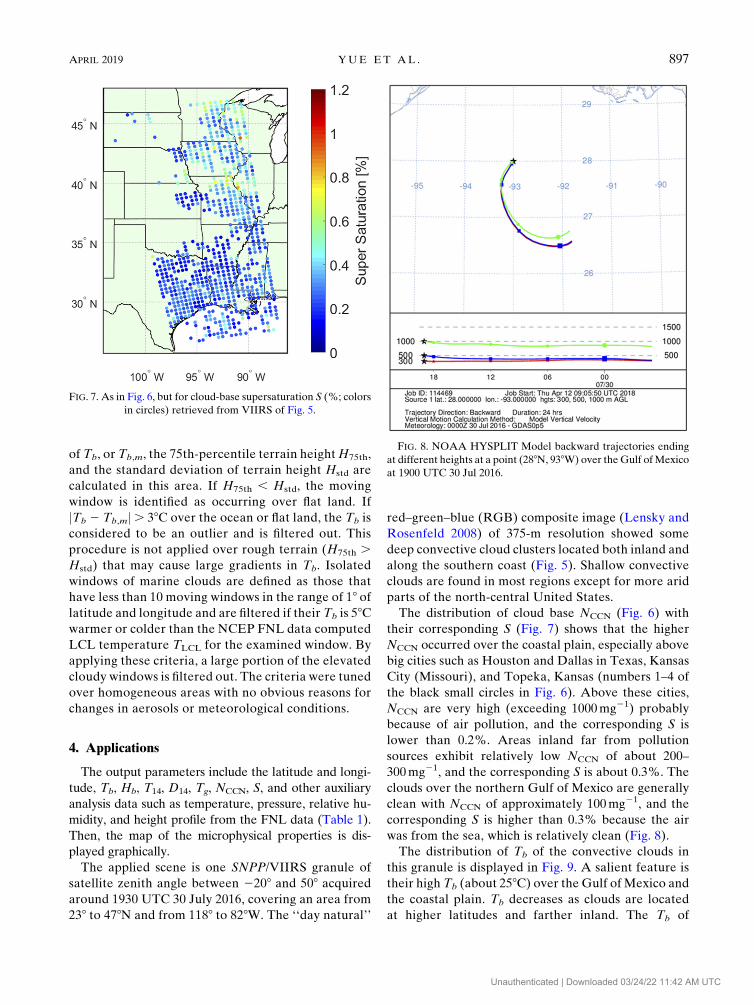
The distribution of cloud base NCCN (Fig. 6) with
their corresponding S (Fig. 7) shows that the higher
NCCN occurred over the coastal plain, especially above
big cities such as Houston and Dallas in Texas, Kansas
City (Missouri), and Topeka, Kansas (numbers 1–4 of
the black small circles in Fig. 6). Above these cities,
NCCN are very high (exceeding 1000mg21) probably
because of air pollution, and the corresponding S is
lower than 0.2%. Areas inland far from pollution
sources exhibit relatively low NCCN of about 200–
300mg21, and the corresponding S is about 0.3%. The
clouds over the northern Gulf of Mexico are generally
clean with NCCN of approximately 100mg21, and the
corresponding S is higher than 0.3% because the air
was from the sea, which is relatively clean (Fig. 8).
The distribution of Tb of the convective clouds in
this granule is displayed in Fig. 9. A salient feature is
their high Tb (about 258C) over the Gulf of Mexico and
the coastal plain. Tb decreases as clouds are located
at higher latitudes and farther inland. The Tb of
FIG. 7. As in Fig. 6, but for cloud-base supersaturation S (%; colors
in circles) retrieved from VIIRS of Fig. 5.
FIG. 8. NOAA HYSPLIT Model backward trajectories ending
at different heights at a point (288N, 938W) over theGulf ofMexico
at 1900 UTC 30 Jul 2016.
APRIL 2019 YUE ET AL . 897
Unauthenticated | Downloaded 03/24/22 11:42 AM UTC
convective clouds above Wisconsin and Minnesota is
between 108 and 158C, while very few of those above the
Midwest are as low as 58C.The cloud-base updraftsWb are
generally low over ocean (0.5–0.8ms21) and are nearly
doubled over land (Fig. 10). The distribution of Wb does
not show excess over the polluted major urban areas with
peakNCCN in Fig. 6. This means that the maxima ofNCCN
can be attributed primarily to the added aerosols and not
to other possible dynamic factors, such as the urban
heat island.
Most D14 (Fig. 11) over the Gulf of Mexico are less
than 500m, suggesting that the cloud forms precipitation
there easily. It shows that most D14 inland exceeds
500m, except for areas with low NCCN. SomeD14 in the
high NCCN inland area are greater than 2000m, in-
dicating that the clouds in these areas are less prone to
producing warm rain.
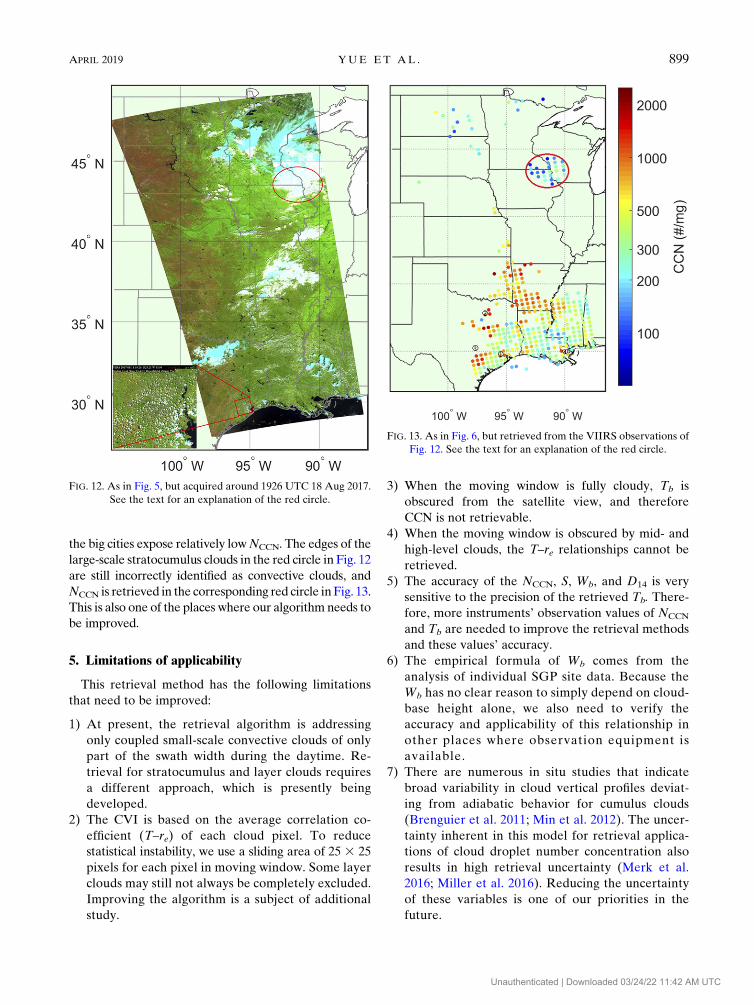
In addition, two retrieval NCCN distributions are
shown below.Many of the small convective clouds are
located in Texas, Louisiana, Mississippi, Arkansas,
and eastern Oklahoma in a day-natural RGB com-
posite image of 375-m resolution on 18 August 2017
acquired around 1926 UTC (Fig. 12). The distribution
of cloud base NCCN (Fig. 13) retrieved from VIIRS of
Fig. 12 shows that the higher NCCN occurred over the
big cities such as Houston (850–1050mg21), Dallas
(1300mg21), south of San Antonio, Texas (950–
1200mg21), and New Orleans, Louisiana (1100mg21)
(numbers 1–4 of the black small circles in Fig. 13).
TheNCCN exceeds 1000mg21 inmany parts of Arkansas
and eastern Oklahoma. Most of the areas in Fig. 14 are
distributed with small convective clouds at 1930 UTC
4 August 2016. The NCCN distribution (Fig. 15) that is
retrieved from Fig. 14 reproduces the distribution of
Figs. 6 and 13. The NCCN over the Gulf of Mexico is
generally 100–500mg21. These regions inland far from
FIG. 9. As in Fig. 6, but for cloud-base temperature Tb (8C; colorsin circles).
FIG. 10. As in Fig. 6, but for cloud-base updraftsWb (m s21; colors
in circles).
FIG. 11. As in Fig. 6, but for precipitation initialization depth D14
(m; colors in circles).
898 JOURNAL OF APPL IED METEOROLOGY AND CL IMATOLOGY VOLUME 58
Unauthenticated | Downloaded 03/24/22 11:42 AM UTC
the big cities expose relatively lowNCCN. The edges of the
large-scale stratocumulus clouds in the red circle in Fig. 12
are still incorrectly identified as convective clouds, and
NCCN is retrieved in the corresponding red circle inFig. 13.
This is also one of the places where our algorithm needs to
be improved.
5. Limitations of applicability
This retrieval method has the following limitations
that need to be improved:
1) At present, the retrieval algorithm is addressing
only coupled small-scale convective clouds of only
part of the swath width during the daytime. Re-
trieval for stratocumulus and layer clouds requires
a different approach, which is presently being
developed.
2) The CVI is based on the average correlation co-
efficient (T–re) of each cloud pixel. To reduce
statistical instability, we use a sliding area of 25 3 25
pixels for each pixel in moving window. Some layer
clouds may still not always be completely excluded.
Improving the algorithm is a subject of additional
study.
3) When the moving window is fully cloudy, Tb is
obscured from the satellite view, and therefore
CCN is not retrievable.
4) When the moving window is obscured by mid- and
high-level clouds, the T–re relationships cannot be
retrieved.
5) The accuracy of the NCCN, S, Wb, and D14 is very
sensitive to the precision of the retrieved Tb. There-
fore, more instruments’ observation values of NCCN
and Tb are needed to improve the retrieval methods
and these values’ accuracy.
6) The empirical formula of Wb comes from the
analysis of individual SGP site data. Because the
Wb has no clear reason to simply depend on cloud-
base height alone, we also need to verify the
accuracy and applicability of this relationship in
other places where observation equipment is
available.
7) There are numerous in situ studies that indicate
broad variability in cloud vertical profiles deviat-
ing from adiabatic behavior for cumulus clouds
(Brenguier et al. 2011; Min et al. 2012). The uncer-
tainty inherent in this model for retrieval applica-
tions of cloud droplet number concentration also
results in high retrieval uncertainty (Merk et al.
2016; Miller et al. 2016). Reducing the uncertainty
of these variables is one of our priorities in the
future.
FIG. 12. As in Fig. 5, but acquired around 1926 UTC 18 Aug 2017.
See the text for an explanation of the red circle.
FIG. 13. As in Fig. 6, but retrieved from the VIIRS observations of
Fig. 12. See the text for an explanation of the red circle.
APRIL 2019 YUE ET AL . 899
Unauthenticated | Downloaded 03/24/22 11:42 AM UTC
8) The retrieval algorithm is not suitable for surface
areas covered with snow or ice because of the lack of
thermal and visible contrast to the clouds.
6. Summary
The latest development of the Automated Mapping
of Convective Clouds is presented in this study. The
AMCC system inputs the VIIRS data and the NCEP
FNL data and produces retrieved maps of NCCN, S, Tb,
Wb, Hb, and D14. It does so with a library of modules of
data processing, image segmentation, moving-window