Automatic pericardium segmentation and quantification of epicardial fat from computed tomography angiography Alexander Norlén Jennifer Alvén David Molnar Olof Enqvist Rauni Rossi Norrlund John Brandberg Göran Bergström Fredrik Kahl Alexander Norlén, Jennifer Alvén, David Molnar, Olof Enqvist, Rauni Rossi Norrlund, John Brandberg, Göran Bergström, Fredrik Kahl, “ Automatic pericardium segmentation and quantification of epicardial fat from computed tomography angiography, ” J. Med. Imag. 3(3), 034003 (2016), doi: 10.1117/1.JMI.3.3.034003.
Transcript
Automatic pericardium segmentationand quantification of epicardial fatfrom computed tomographyangiography
Alexander NorlénJennifer AlvénDavid MolnarOlof EnqvistRauni Rossi NorrlundJohn BrandbergGöran BergströmFredrik Kahl
Alexander Norlén, Jennifer Alvén, David Molnar, Olof Enqvist, Rauni Rossi Norrlund, John Brandberg,Göran Bergström, Fredrik Kahl, “Automatic pericardium segmentation and quantification of epicardial fatfrom computed tomography angiography,” J. Med. Imag. 3(3), 034003 (2016),doi: 10.1117/1.JMI.3.3.034003.
Automatic pericardium segmentation andquantification of epicardial fat from computedtomography angiography
Alexander Norlén,a Jennifer Alvén,a,* David Molnar,b Olof Enqvist,b Rauni Rossi Norrlund,b John Brandberg,bGöran Bergström,b and Fredrik Kahla,caChalmers University of Technology, Department of Signals and Systems, Hörsalsvägen 9-11, Gothenburg 412 96, SwedenbGothenburg University, Sahlgrenska Academy, Institute of Medicine, The Wallenberg Laboratory, Bruna stråket 16, Gothenburg 413 45, SwedencLund University, Faculty of Engineering, Centre for Mathematical Sciences, Sölvegatan 18, Lund 221 00, Sweden
Paper 16037RR received Mar. 3, 2016; accepted for publication Aug. 29, 2016; published online Sep. 15, 2016.
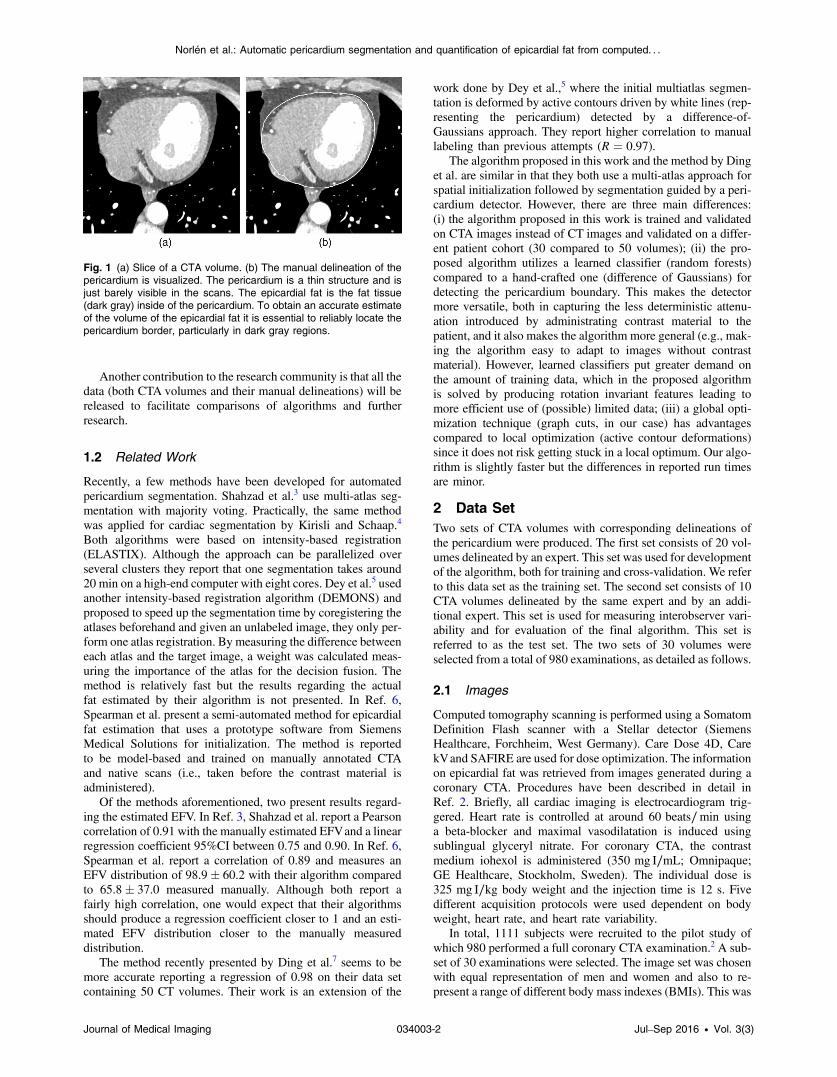
1 IntroductionVisceral adipose tissue, i.e., fat surrounding the internal organs,may be a marker for increased risk of different metabolic andcardiovascular diseases. Epicardial fat is the visceral fat depotenclosed by the pericardial sac. In other words, it is the fat locatedaround the heart but inside of the pericardial sac that surroundsthe heart (see Fig. 1). In recent years, several studies have shown arelationship between increased volume of epicardial fat and coro-nary artery disease, coronary plaque, adverse cardiovascularevents, myocardial ischemia, and atrial fibrillation.1 However,due to technical limitations in three-dimensional (3-D) segmen-tation of epicardial fat the studies are of limited size and infor-mation on the prognostic value of epicardial fat for developmentof ischemic heart disease is scarce.
The Swedish CardioPulmonary Bioimage Study2 (SCAPIS)is a nationwide research project that started in 2012 in a collabo-ration between six universities in Sweden and their universityhospitals. It is a large-scale study that aims at collecting CT,MR, and ultrasound images from 30,000 men and womenbetween 50 and 64 years of age. This database gives an oppor-tunity to investigate the importance of epicardial fat as a riskmarker for heart disease. Hence, there is a need for a fully auto-mated method for epicardial fat quantification that is suitable fora study of this magnitude.
In this paper, an efficient method for pericardium segmenta-tion and epicardial fat volume (EFV) estimation from computedtomography angiography (CTA) is presented. The algorithmuses efficient feature-based multiatlas registrations for spatialinitialization. Thereafter, the pericardium is detected by random
forest classification and then the target image is segmented aseither inside or outside of the pericardium by global optimiza-tion through graph cuts. Finally, the amount of epicardial fat canbe quantified by combining thresholding with the pericardiumlabeling. Our experimental results on pericardium segmentationand EFVestimation show that the algorithm yields very accuratesegmentations and significantly outperforms previous results onpericardium segmentation with run-times suitable for large-scalestudies. More importantly, the measurement errors comparefavorably to the interobserver variability measured on a setof 10 patients delineated by two medical experts using thesame time-consuming and accurate method for delineation.
1.1 Contributions
The main contribution of this work is an algorithm that effi-ciently produces accurate EFV estimations from CTA images,making large-scale studies of the relationship between epicardialfat and heart disease tractable.
The primary algorithmic contribution is how a generalizedformulation of multi-atlas segmentation based on distancemaps is incorporated into a random forest classification frame-work. More specifically, the voxel-wise distribution of the dis-tance to the boundary of the region of interest is used to producerotation invariant features for the random forest classifier, effec-tively reducing the dimensionality of the classification problemfrom three dimensions to one. This not only makes the processof classification easier but also normalizes the training data lead-ing to more efficient use of the (often in medical image analysis)limited labeled data set.
Another contribution to the research community is that all thedata (both CTA volumes and their manual delineations) will bereleased to facilitate comparisons of algorithms and furtherresearch.
1.2 Related Work
Recently, a few methods have been developed for automatedpericardium segmentation. Shahzad et al.3 use multi-atlas seg-mentation with majority voting. Practically, the same methodwas applied for cardiac segmentation by Kirisli and Schaap.4
Both algorithms were based on intensity-based registration(ELASTIX). Although the approach can be parallelized overseveral clusters they report that one segmentation takes around20 min on a high-end computer with eight cores. Dey et al.5 usedanother intensity-based registration algorithm (DEMONS) andproposed to speed up the segmentation time by coregistering theatlases beforehand and given an unlabeled image, they only per-form one atlas registration. By measuring the difference betweeneach atlas and the target image, a weight was calculated meas-uring the importance of the atlas for the decision fusion. Themethod is relatively fast but the results regarding the actualfat estimated by their algorithm is not presented. In Ref. 6,Spearman et al. present a semi-automated method for epicardialfat estimation that uses a prototype software from SiemensMedical Solutions for initialization. The method is reportedto be model-based and trained on manually annotated CTAand native scans (i.e., taken before the contrast material isadministered).
Of the methods aforementioned, two present results regard-ing the estimated EFV. In Ref. 3, Shahzad et al. report a Pearsoncorrelation of 0.91 with the manually estimated EFVand a linearregression coefficient 95%CI between 0.75 and 0.90. In Ref. 6,Spearman et al. report a correlation of 0.89 and measures anEFV distribution of 98.9� 60.2 with their algorithm comparedto 65.8� 37.0 measured manually. Although both report afairly high correlation, one would expect that their algorithmsshould produce a regression coefficient closer to 1 and an esti-mated EFV distribution closer to the manually measureddistribution.
The method recently presented by Ding et al.7 seems to bemore accurate reporting a regression of 0.98 on their data setcontaining 50 CT volumes. Their work is an extension of the
work done by Dey et al.,5 where the initial multiatlas segmen-tation is deformed by active contours driven by white lines (rep-resenting the pericardium) detected by a difference-of-Gaussians approach. They report higher correlation to manuallabeling than previous attempts (R ¼ 0.97).
The algorithm proposed in this work and the method by Dinget al. are similar in that they both use a multi-atlas approach forspatial initialization followed by segmentation guided by a peri-cardium detector. However, there are three main differences:(i) the algorithm proposed in this work is trained and validatedon CTA images instead of CT images and validated on a differ-ent patient cohort (30 compared to 50 volumes); (ii) the pro-posed algorithm utilizes a learned classifier (random forests)compared to a hand-crafted one (difference of Gaussians) fordetecting the pericardium boundary. This makes the detectormore versatile, both in capturing the less deterministic attenu-ation introduced by administrating contrast material to thepatient, and it also makes the algorithm more general (e.g., mak-ing the algorithm easy to adapt to images without contrastmaterial). However, learned classifiers put greater demand onthe amount of training data, which in the proposed algorithmis solved by producing rotation invariant features leading tomore efficient use of (possible) limited data; (iii) a global opti-mization technique (graph cuts, in our case) has advantagescompared to local optimization (active contour deformations)since it does not risk getting stuck in a local optimum. Our algo-rithm is slightly faster but the differences in reported run timesare minor.
2 Data SetTwo sets of CTA volumes with corresponding delineations ofthe pericardium were produced. The first set consists of 20 vol-umes delineated by an expert. This set was used for developmentof the algorithm, both for training and cross-validation. We referto this data set as the training set. The second set consists of 10CTA volumes delineated by the same expert and by an addi-tional expert. This set is used for measuring interobserver vari-ability and for evaluation of the final algorithm. This set isreferred to as the test set. The two sets of 30 volumes wereselected from a total of 980 examinations, as detailed as follows.
2.1 Images
Computed tomography scanning is performed using a SomatomDefinition Flash scanner with a Stellar detector (SiemensHealthcare, Forchheim, West Germany). Care Dose 4D, CarekVand SAFIRE are used for dose optimization. The informationon epicardial fat was retrieved from images generated during acoronary CTA. Procedures have been described in detail inRef. 2. Briefly, all cardiac imaging is electrocardiogram trig-gered. Heart rate is controlled at around 60 beats∕min usinga beta-blocker and maximal vasodilatation is induced usingsublingual glyceryl nitrate. For coronary CTA, the contrastmedium iohexol is administered (350 mg I∕mL; Omnipaque;GE Healthcare, Stockholm, Sweden). The individual dose is325 mg I∕kg body weight and the injection time is 12 s. Fivedifferent acquisition protocols were used dependent on bodyweight, heart rate, and heart rate variability.
In total, 1111 subjects were recruited to the pilot study ofwhich 980 performed a full coronary CTA examination.2 A sub-set of 30 examinations were selected. The image set was chosenwith equal representation of men and women and also to re-present a range of different body mass indexes (BMIs). This was
Fig. 1 (a) Slice of a CTA volume. (b) The manual delineation of thepericardium is visualized. The pericardium is a thin structure and isjust barely visible in the scans. The epicardial fat is the fat tissue(dark gray) inside of the pericardium. To obtain an accurate estimateof the volume of the epicardial fat it is essential to reliably locate thepericardium border, particularly in dark gray regions.
Journal of Medical Imaging 034003-2 Jul–Sep 2016 • Vol. 3(3)
Norlén et al.: Automatic pericardium segmentation and quantification of epicardial fat from computed. . .
deemed suitable since EFV correlates with BMI. Demographicsof these subjects are shown in Table 1. The images have reso-lutions ranging between 512 × 512 × 342 and 512 × 512 × 458voxels with voxel dimensions between 0.32 × 0.32 × 0.30 mm3
and 0.43 × 0.43 × 0.30 mm3.The study was approved by the ethics committee at Umeå
University and adheres to the Declaration of Helsinki. Informedconsent was collected from all subjects.2
2.2 Manual Delineations
The manual delineations were done by two medical experts,both specialists in thoracic radiology. The pericardium wasdelineated on every 10th slice in the three standard orthogonalplanes (axial, coronal, and sagittal) independently. Delineationin two dimensions was preferred to a possible method of seg-menting directly in three dimensions to (i) ensure maximal ana-tomical precision, as radiologists are more comfortable withviewing structures in two dimensions at a time, (ii) be ableto precisely reproduce the circumstances for the two experts.The same slices were delineated by both experts.
During segmentation, if the pericardium was not clearly vis-ible in parts of the actual slice, a decision was made where thepericardium was most probably located based on the neighbor-ing slices and the experts’ anatomical knowledge. This approachwas particularly useful in the areas where many different ana-tomical structures are close to each other, e.g., the diaphragmalsurface of the pericardium.
Delineation in all three planes was mainly done because ofthe problem of delineating structures parallel to the plane ofviewing, resulting in poor accuracy in these areas. The slice-wise segmentations, made in each orthogonal plane independ-ently, were interpolated into three volumes. The final resultingvolume was computed as the volume where two out of the threevolumes overlapped, assuming that this would reduce the error,mainly stemming from the problem of tangential delineationmentioned above. The final volume was approved by the expert.We refer to the manual labeling as the gold standard.
3 MethodThe developed algorithm consists of three main parts. The firstpart is the spatial initialization (Sec. 3.1) using efficient feature-based multi-atlas techniques. This first part serves as a globalinitialization for pericardium localization, reducing the needfor an explicit shape model. A variant of multi-atlas representa-tion (denoted as MADMAP) provides valuable information ofthe certainty of the voxels being inside or outside of the
pericardium. With this information, we can limit the pericar-dium search space to a small region around the pericardiumsurface.
The second part of the algorithm is the pericardium detection(Sec. 3.2). A random forest classifier is trained on the labeledatlas set to accurately detect the pericardium. The extractedimage features used for training and classification are alignedalong a direction estimated from the MADMAP to beperpendicular to the pericardium, practically reducing the peri-cardium detection problem to a line search. This approach alsoexpands the effectively used amount of training data because itlets the forest learn what a pericardial neighborhood looks likeirrespective of how it is oriented toward the image coordinateaxes (an important consideration in medical image analysiswhere manually labeled data rarely is abundant). The classifieris trained to distinguish between four classes:
1. just inside of the pericardium,
2. just at the pericardium boundary,
3. just outside of the pericardium,
4. everything else.
This makes detailed information of what the boundary lookslike available to the forest during training and produces a clas-sifier with a high discriminating power.
The final part is segmentation (Sec. 3.3). The informationfrom the global spatial initialization and from local and indepen-dent posteriors estimated by the random forest classifier is com-bined into a Markov random field (MRF). The globally optimalsegmentation is computed through graph cuts. Figure 2 summa-rizes the main parts of the algorithm.
3.1 Spatial initialization
Multiatlas segmentation (see for example Ref. 8), which is usedby almost all previous methods for pericardium segmentation(including this one), is a widely used method for organ segmen-tation in medical image analysis. An atlas is an image with acorresponding labeling L. Standard multiatlas segmentationinvolves registering each atlas image to the target image, fol-lowed by transferring the atlas labeling to produce a vote map.The proposed algorithm includes a spatial initialization includ-ing feature-based registration and a generalized representationof the standard multiatlas vote map.
3.1.1 Feature-based registration
In medical applications, the registration methods are typicallyintensity-based and nonrigid, e.g., as in Ref. 3, which tend tobe computationally very demanding. As our intention is toapply our framework to thousands of images, a more efficientmethod is required. In contrast to intensity-based methods, fea-ture-based registration is less common in medical image analy-sis due to the conception that it is hard to detect salient featuresin medical images. However, as was shown by Svärm et al.,9
feature-based registration based on robust optimization tech-niques outperforms a variety of intensity-based methods in esti-mating affine transformations for whole-body CT scans as wellas brain MR scans. Feature-based registration was both moreefficient and less likely to produce large errors.
We use a 3-D version of the difference-of-Gaussians detectorin SIFT10 together with the descriptor from SURF.11 We use
Table 1 Demographics of the subjects present in the data sets usedfor training and evaluation of the algorithm.
Variable Training set Test set Total
N 20 10 30
Sex, female (n, %) 10 (50) 5 (50) 15 (50)
Age (median, range) 57 (51 to 65) 58 (50 to 65) 57 (50 to 65)
BMI (median, range) 27.4 (17.4 to40.2)
30.1 (17.9 to40.1)
28.0 (17.4 to40.2)
Journal of Medical Imaging 034003-3 Jul–Sep 2016 • Vol. 3(3)
Norlén et al.: Automatic pericardium segmentation and quantification of epicardial fat from computed. . .
rotation invariant features. The features are matched between theimages using the ratio criterion used by Ref. 10, referred to asthe Lowe criterion, i.e., we discard matches where the ratio ofthe distance from the closest neighbor to the distanceof the second closest are larger than a threshold. Given thematch hypotheses, RANSAC12 is used to obtain the matchesthat are approximately consistent with an affine transformation.RANSAC is run with the l1-norm (truncated at a threshold) as acost function and with 50,000 iterations. Only unique matchesare allowed. If there is a matching conflict, then the match that isclosest in descriptor space is used. Through this process a set ofmatches, mostly cleared from outliers, is obtained. We only usefeatures in the atlas images that are within 10 mm or inside of thepericardium, thus completely ignoring other anatomical regionsin the atlases.
Finally, the nonrigid deformations around the heart are esti-mated by registering the final feature matches (the ones consid-ered as inliers by the RANSAC algorithm). We represent thedeformations with B-spline and use an implementation basedon the registration algorithm by Ref. 13 with a final B-splinegrid size of 4 mm.
3.1.2 Multi-atlas distance map
The MADMAP is a generalized representation of the standardmulti-atlas vote map. What is usually done is that the (binary)
manually labeled images produced by the experts are trans-formed into the space of the target image resulting in a votemap where the information at each voxel is the number of atlasesthat vote for this voxel being inside or outside of the region ofinterest. Exactly the same procedure is used here with the modi-fication that instead of the atlas labels, the signed distances to thepericardium are transformed into the space of the target image.A similar approach was proposed in Ref. 14.
The proposed approach is a minor change to the standard onebut it results in a major information gain regarding the multi-atlas registrations at no extra computational cost. For eachvoxel, the atlases vote for the signed distance to the boundaryof the region of interest. Not only does this give us the possibil-ity of estimating the actual distance to the real boundary, we alsoobtain a voxel-wise measure of uncertainty of the estimatedsigned distance (and by extension a measure of uncertaintyof the atlas registrations around the voxel) by measuring thevariance of the votes. This approach generalizes the standardmulti-atlas voting procedure; the standard votes are obtainedas a special case by only counting negative votes, e.g., majorityvoting fusion is obtained as all voxels where the median of thevotes is less than zero.
The MADMAP (denoted M) is the object containing all dis-tance votes. In this work, we use a compact representation of theMADMAP where we only save the voxel-wise median of thevotes (denoted M̃) and the voxel-wise mean absolute deviation
(a) (b)
(c) (d)
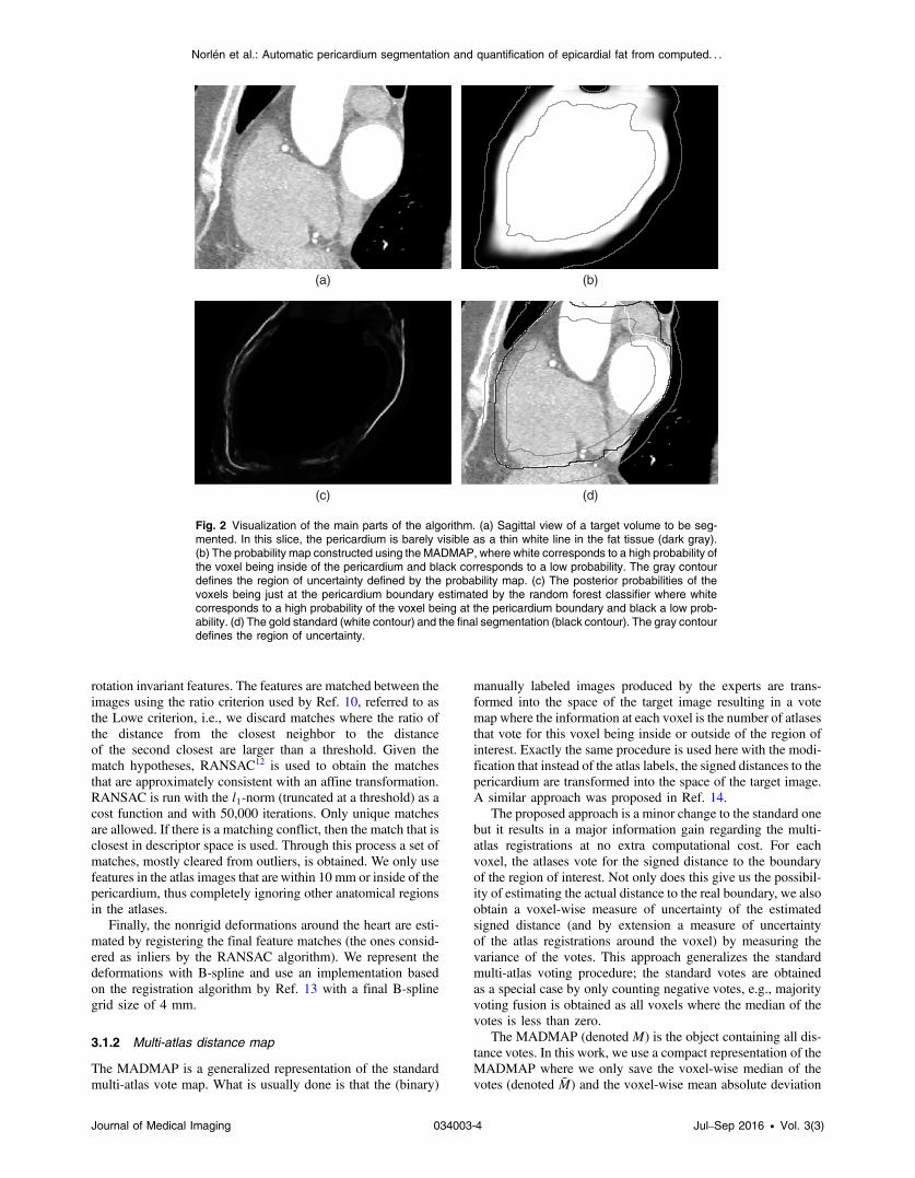
Fig. 2 Visualization of the main parts of the algorithm. (a) Sagittal view of a target volume to be seg-mented. In this slice, the pericardium is barely visible as a thin white line in the fat tissue (dark gray).(b) The probability map constructed using the MADMAP, where white corresponds to a high probability ofthe voxel being inside of the pericardium and black corresponds to a low probability. The gray contourdefines the region of uncertainty defined by the probability map. (c) The posterior probabilities of thevoxels being just at the pericardium boundary estimated by the random forest classifier where whitecorresponds to a high probability of the voxel being at the pericardium boundary and black a low prob-ability. (d) The gold standard (white contour) and the final segmentation (black contour). The gray contourdefines the region of uncertainty.
Journal of Medical Imaging 034003-4 Jul–Sep 2016 • Vol. 3(3)
Norlén et al.: Automatic pericardium segmentation and quantification of epicardial fat from computed. . .
from the median (denotedD½M�). We refer to this representationas the l1-norm representation of M. We also validate the accu-racy of the algorithm when using the l2-norm, i.e., the voxel-wise mean and standard deviation of the distance votes. For sim-plicity, the l1-norm notation is used for the rest of the presen-tation of this algorithm.
The median ~M is an estimation of the distance transform ofthe pericardium in the target image. The median ~M and thedeviation D½M� are used to compute a probability of a locationp being inside Prðp ∈ LjMÞ or outside Prðp ∈ LjMÞ of thepericardium by assuming a normally distributed measurementerror. This probability map is used to define a region of uncer-tainty, i.e., locations that are not definitely inside and not def-initely outside according to the MADMAP. For efficiency, thepericardium search is limited to this region. For a visualization,see Fig. 2(b).
3.2 Pericardium Detection
Multi-atlas registration is a robust method for spatial estima-tion of where the pericardium is approximately located. Butsince the pericardium does not constitute a clearly visibleboundary for the region of interest, which would guide theregistrations, the actual placement of the segmentation boun-dary will not be accurate. Therefore, we train a boundary detec-tor that, given the spatial initialization from MADMAP, willrespond to the image features that resemble the pericardiumsurface.
The boundary detector is based on random decisionforests,15,16 a machine learning technique suitable for this clas-sification tasks since it generalizes well to unseen data, naturallyextends to multiclass classification problems and is computa-tionally efficient.
3.2.1 Training
The forest is trained to distinguish between four classes. Justinside of the pericardium (between −1.5 and −0.5 mm fromthe pericardium), just at the pericardium boundary (−0.5 to
0.5 mm), just outside of the pericardium (0.5 to 1.5 mm) andbackground (any other location between −8 and 8 mm).These classes are denoted c ∈ fin; on; out; bgg. An equalamount of locations are randomly sampled from each classand the corresponding features are extracted. The axis alignedsplitting function is used where the splitting function is definedas a hyperplane aligned along one of the axes. The hyperplane isdefined by the axis and a threshold. The splitting functions arechosen as the function that maximizes the information gain(Shannon entropy). For training, a total of 40 million data pointswere extracted, evenly distributed over the classes and theatlases.
3.2.2 Features
The feature vector [the data point ~vðpÞ extracted at location p]consists of mean values and l1-variance of the image intensitiesand first- and second-order derivatives and gradient magnitudesof the image intensities, extracted from local regions around p.The regions are oriented along the normal direction of the peri-cardium surface as predicted byMADMAP, effectively reducingthe dimensionality of the classification problem from threedimensions to one.
The feature elements at a location p are computed as follows.Let G ¼ fGi;j;kg3i;j;k¼1
be an equidistant 3 × 3 × 3 grid of pointscentered at the origin. The spacing between the points is 1 mm.Let R be the rotation that aligns the third dimension of G(indexed by k) with the gradient of M̃ at p. Let Si;j;k ¼ IðpþR ∘ sGi;j;kÞ be the intensities of the image I sampled at the loca-tion specified by the grid pointGi;j;k (which has been centered atlocation p, scaled by a factor s, and rotated along the MADMAPgradient). A set of local image statistics Tðp; I; sÞ consists of
Mean: m ¼ ð1∕27ÞP3i;j;k¼1 Si;j;k and
P3i;j;k¼1 jSi;j;k −mj,
Means: mk ¼ ð1∕9ÞP3i;j¼1 Si;j;k and
P3i;j¼1 jmk − Si;j;kj,
k ¼ f1; 2; 3g,First gradient:
P2k¼1
P3i;j¼1 Si;j;kþ1 − Si;j;k andP
2k¼1
P3i;j¼1 jSi;j;kþ1 − Si;j;kj,
(a) (b) (c)
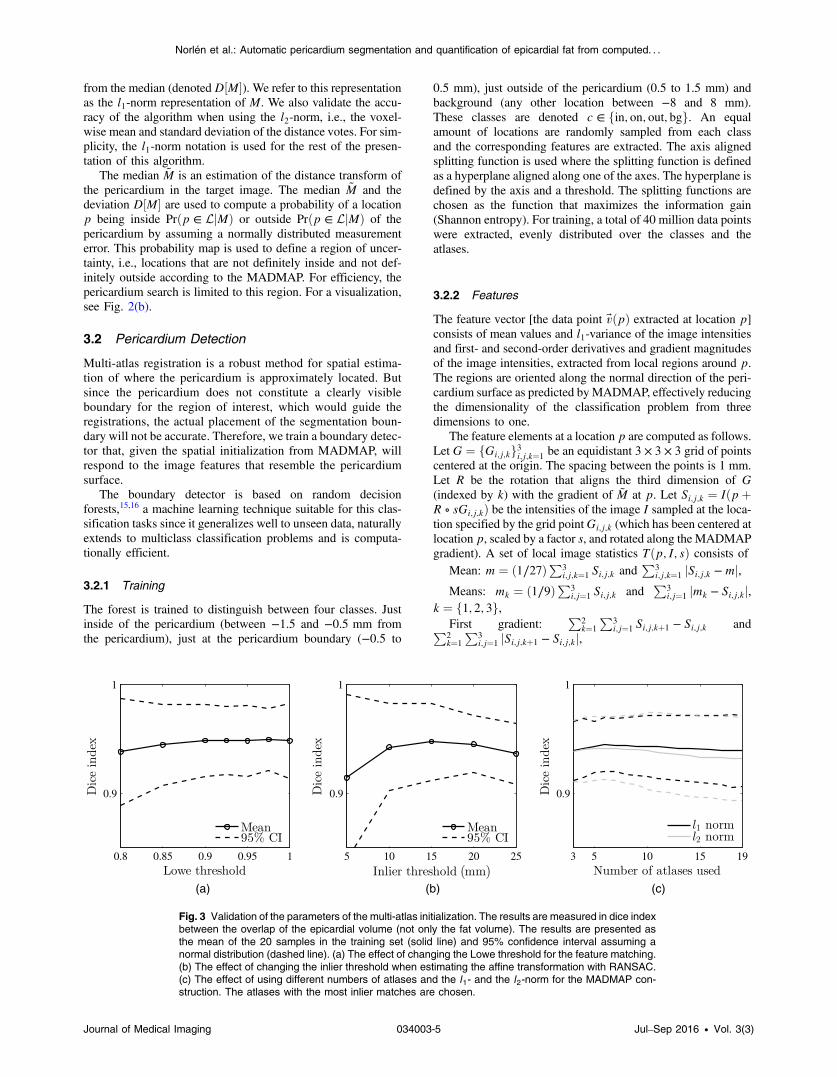
Fig. 3 Validation of the parameters of the multi-atlas initialization. The results are measured in dice indexbetween the overlap of the epicardial volume (not only the fat volume). The results are presented asthe mean of the 20 samples in the training set (solid line) and 95% confidence interval assuming anormal distribution (dashed line). (a) The effect of changing the Lowe threshold for the feature matching.(b) The effect of changing the inlier threshold when estimating the affine transformation with RANSAC.(c) The effect of using different numbers of atlases and the l1- and the l2-norm for the MADMAP con-struction. The atlases with the most inlier matches are chosen.
Journal of Medical Imaging 034003-5 Jul–Sep 2016 • Vol. 3(3)
Norlén et al.: Automatic pericardium segmentation and quantification of epicardial fat from computed. . .
First gradients:P
3i;j¼1 Si;j;kþ1 − Si;j;k andP
3i;j¼1 jSi;j;kþ1 − Si;j;kj, k ¼ f1; 2g,Second-order derivative:
P3i;j¼1 −Si;j;3 þ 2Si;j;2 − Si;j;1 andP
3i;j¼1 j − Si;j;3 þ 2Si;j;2 − Si;j;1j.The features are sampled from the CT volume I0, the same
volume filtered with a Gaussian kernel with σ ¼ 1 mm (I1) andwith σ ¼ 2 mm (I2). The complete list of features extractedfrom each location p is I0ðpÞ, I1ðpÞ, I2ðpÞ, Tðp; I0; 1Þ,Tðp; I0; 1.5Þ, Tðp; I1; 1.5Þ, Tðp; I1; 2Þ, Tðp; I2; 2Þ, andTðp; I2; 3Þ. A total of 99 features.
3.3 Segmentation
By viewing the image I as an observation of a MRF17,18 and therealization of the field as the labeling L� of the voxels, the label-ing that maximizes the a posteriori probability can be inferredby minimizing an energy function of the form
where P is the set of all pixels (or voxels) in the image andN isthe set of all neighbors. Here Vp is referred to as the unary costand Vp;q the pairwise cost. A function on this form can be for-mulated as a weighted graph G ¼ hV; Ei. If E in Eq. (1) is sub-modular, the globally optimal segmentation L� can be computedin polynomial time.
The MADMAP has been used to compute the probability ofa location being inside Prðp ∈ LjMÞ or outside Prðp ∈= LjMÞ ofthe pericardium and a six-connected graph is constructed overthe region of uncertainty. The set of locations PV correspondingto the nodes V in the graph are classified by the random forestproducing a distribution Pr½p ∈ cj~vðpÞ� over the set of classesc ∈ C, for each p ∈ PV . Figure 2(c) presents an example ofwhat Pr½p ∈ onj~vðpÞ� can look like. To control the amountof influence, the MADMAP probabilities have on the final seg-mentation, we introduce the parameter μ and define the parame-terized MADMAP probability Min as
EQ-TARGET;temp:intralink-;e002;326;432MinðpÞ ¼ 1
1þ�Prðp∈=LjMÞPrðp∈LjMÞ
�1μ
: (2)
The unary costs of the MRF energy function in Eq. (1) aredefined as
Table 2 Result comparison between the proposed method versusExpert 1 and Expert 2 versus Expert 1.
Proposed versusExpert 1
Expert 2 versusExpert 1
Mean absolute EFVdifference (ml)
2.68 5.10
Median absolute EFVdifference (ml)
2.22 3.82
EFV (ml) (Expert 1:108.44� 74.65)
109.22� 75.11 103.34� 74.82
Pearson correlation 0.9989 0.9986
Linear regressioncoefficient (95% CI)
1.01 (0.97, 1.04) 1.00 (0.96, 1.04)
Bland–Altman bias (ml)(95% CI)
0.78 (−6.31, 7.86) −5.10 (−12.88,2.67)
Dice (mean� std) 0.91� 0.04 0.90� 0.04
Dice total volume(mean� std)
0.97� 0.01 0.98� 0.00
Note: The comparisons are of the measured EFV in all cases exceptfor dice total volume, where the overlap of the total epicardial volumeis measured.
(a) (b) (c) (d)
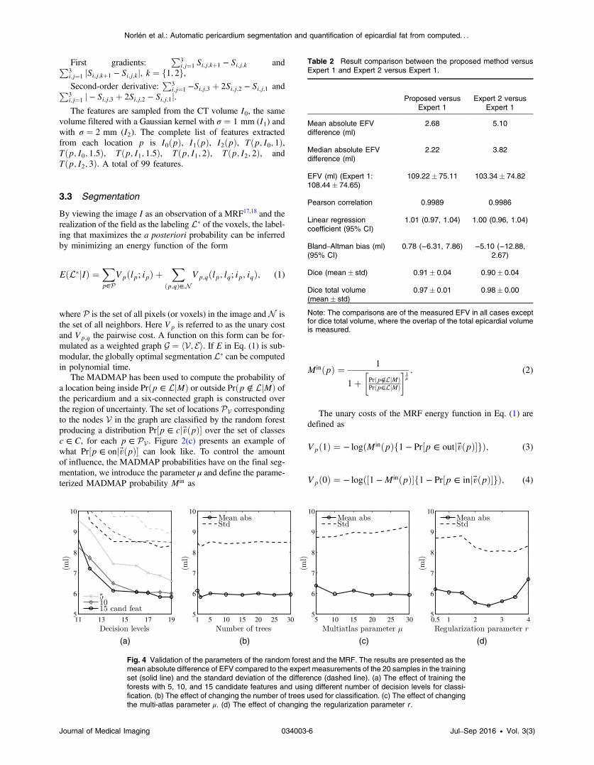
Fig. 4 Validation of the parameters of the random forest and the MRF. The results are presented as themean absolute difference of EFV compared to the expert measurements of the 20 samples in the trainingset (solid line) and the standard deviation of the difference (dashed line). (a) The effect of training theforests with 5, 10, and 15 candidate features and using different number of decision levels for classi-fication. (b) The effect of changing the number of trees used for classification. (c) The effect of changingthe multi-atlas parameter μ. (d) The effect of changing the regularization parameter r .
Journal of Medical Imaging 034003-6 Jul–Sep 2016 • Vol. 3(3)
Norlén et al.: Automatic pericardium segmentation and quantification of epicardial fat from computed. . .
where for shorthand notation, we have excluded the obviousdependence on I. In other words, the cost of assigning anode to inside the pericardium is small if the probability ofp being inside is large according to the MADMAP and if theprobability of p being just outside of the pericardium issmall according to the random forest.
For each edge fp; qg ∈ E, we define its location as thelocation between the nodes connected by the edge, i.e.,ðpþ qÞ∕2. It is classified by the random forest and we infera probability of the edge being on the pericardium boundary,Prfðpþ qÞ∕2 ∈ onj~v½ðpþ qÞ∕2�g. The pairwise costs are thendefined as
Two parameters are introduced, the regularization r control-ling the weighting between the unary and the pairwise costs and
the uncertainty threshold τ that specifies the maximum cost foran edge. Nodes with infinite unary costs are appended directlyon the inside and outside of the region of uncertainty, forcing theboundary into this region.
The final segmentation L� is chosen as the max-flow/min-cutover the graph [see Fig. 2(d)] and is inferred using the max-flowalgorithm,19 which is a widely used method in computer vision.
3.4 Hyperparameter Optimization
The algorithm was validated using leave-one-out on the trainingset consisting of 20 CTA volumes of the heart and the corre-sponding gold standard.
The validation was first done on the hyperparameters of theMADMAP. A MADMAP was constructed for each of theimages by registering the remaining atlases affinely to the targetimage. The atlases with the most inlier matches were registerednonrigidly and their distance transforms were subsequentlypropagated to the target image. The parameters of the registra-tions were optimized against the mean dice index of the total
(a) (b)
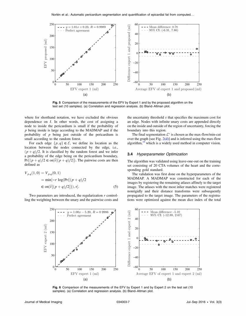
Fig. 5 Comparison of the measurements of the EFV by Expert 1 and by the proposed algorithm on thetest set (10 samples). (a) Correlation and regression analysis. (b) Bland–Altman plot.
(a) (b)
Fig. 6 Comparison of the measurements of the EFV by Expert 1 and by Expert 2 on the test set (10samples). (a) Correlation and regression analysis. (b) Bland–Altman plot.
Journal of Medical Imaging 034003-7 Jul–Sep 2016 • Vol. 3(3)
Norlén et al.: Automatic pericardium segmentation and quantification of epicardial fat from computed. . .
epicardial volume computed between the region, where themedian of the MADMAP was less than 0 (equivalent to majorityvoting in standard multiatlas segmentation) and the goldstandard.
The best MADMAPs were then used as initialization forvalidating the hyperparameters of the pericardium detectionand segmentation. The hyperparameters of the random forestand the MRF used for the final segmentation of the imageswere optimized against the mean absolute EFV difference.For each image, the algorithm was trained on the remainingimages.
3.5 Epicardial Fat Volume Quantification
The intensity values of the voxels in a CTA image corresponddirectly to Hounsfield units (HU). Usually, the fat in the image isfound by simple thresholding. In this work, fat is defined as allvoxels with an attenuation between −192 and −30 HU,20 whichcombined with the pericardium segmentation allows for quan-tification of the EFV.
4 Experiments and Results
4.1 Hyperparameter Optimization
Figure 3 presents some results from the MADMAP hyperpara-meter optimization. As can be seen, the results are not sensitiveto the choice of Lowe threshold for the matching [see Fig. 3(a)].A threshold of 0.975 was chosen for the Lowe criterion. Theoutlier matches were handled by RANSAC, where the inlierthreshold was chosen to 15 mm [Fig. 3(b)]. Finally, we evalu-ated the effect of only using the atlases with the most inliermatches for the nonrigid registration and looked at the effectsof using the mean of the MADMAP instead of the median(l2 instead of l1). The results are presented in Fig. 3(c).Interestingly, by only using a few of the atlases for the final con-struction of the MADMAP, the initialization gets slightly morerobust and of course it makes it more efficient. Also, the l1-normslightly outperforms the l2-norm, especially when using moreatlases. The l1-norm and using the six atlases with most inlierswere chosen for the final parameter set. The region of uncer-tainty is defined as the region where either jM̃ðpÞj < 8 mmor 0.0001 < Prðp ∈ LjMÞ < 0.9999.
Figure 4 shows some results obtained during the random for-est and MRF hyperparameter optimization. The forest wastrained using 5, 10, and 15 candidate features (the size of therandom subsets of features used for optimization of the splittingfunctions). About 15 candidate features and 19 decision levels,the maximum allowed depth allowed by the current implemen-tation, were chosen [see Fig. 4(a)]. Overtraining did not seem tobe a concern. Interestingly, when the trees were trained in thismanner, one obtains the same results with just a few trees [seeFig. 4(b)]. In fact, the results were stable using only one tree in
(a) (b)
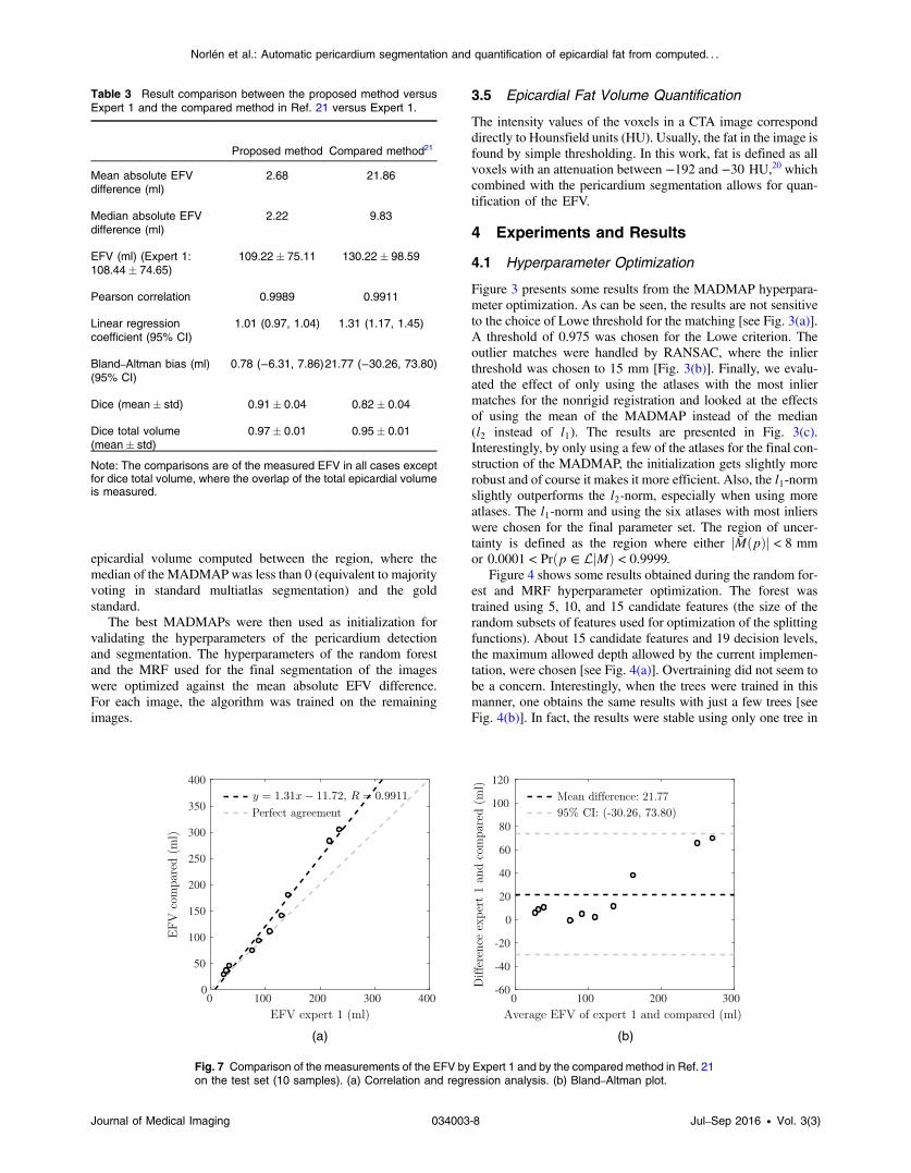
Fig. 7 Comparison of the measurements of the EFV by Expert 1 and by the compared method in Ref. 21on the test set (10 samples). (a) Correlation and regression analysis. (b) Bland–Altman plot.
Table 3 Result comparison between the proposed method versusExpert 1 and the compared method in Ref. 21 versus Expert 1.
Proposed method Compared method21
Mean absolute EFVdifference (ml)
2.68 21.86
Median absolute EFVdifference (ml)
2.22 9.83
EFV (ml) (Expert 1:108.44� 74.65)
109.22� 75.11 130.22� 98.59
Pearson correlation 0.9989 0.9911
Linear regressioncoefficient (95% CI)
1.01 (0.97, 1.04) 1.31 (1.17, 1.45)
Bland–Altman bias (ml)(95% CI)
0.78 (−6.31, 7.86)21.77 (−30.26, 73.80)
Dice (mean� std) 0.91� 0.04 0.82� 0.04
Dice total volume(mean� std)
0.97� 0.01 0.95� 0.01
Note: The comparisons are of the measured EFV in all cases exceptfor dice total volume, where the overlap of the total epicardial volumeis measured.
Journal of Medical Imaging 034003-8 Jul–Sep 2016 • Vol. 3(3)
Norlén et al.: Automatic pericardium segmentation and quantification of epicardial fat from computed. . .
the forests. To be sure, we chose 10 trees for the final param-eter set.
The graph was not constructed directly on the voxels of theimage but was first downsampled. An isometric node spacing of1 mm made the algorithm more efficient and at the same timeproved to provide enough detail to not affect the accuracy of thesegmentation. The algorithm was not very sensitive to the multi-atlas parameter μ [see Fig. 4(c)] and it was set to 20. The pair-wise cost parameters r and τ were set to 2.5 and 10, respectively.The effect of different r can be seen in Fig. 4(d).
4.2 Pericardium Segmentation and Epicardial FatVolume Estimation
The proposed algorithm was trained on the 20 atlases in thetraining set and tested on the 10 samples in the test set,which were unseen during development of the algorithm. Thepericardium in each of the 10 test samples was manually
delineated by the same expert (Expert 1) who delineated thesamples in the training set and by another expert (Expert 2)for interobserver comparisons. The results are presented inTable 2. Regression analysis and Bland–Altman plots betweenthe proposed method and Expert 1 and between Expert 2 andExpert 1 are visualized in Figs. 5 and 6, respectively. The aver-age total segmentation time was 51.9 s (Intel Core [email protected] with 6 cores).
4.3 Comparison to State-of-the-Art SegmentationMethod
In addition, our method was compared to the multiatlas-basedsegmentation described in Ref. 21 (using joint label fusion withcorrective learning). Their method won the first place of themultiatlas labeling challenge at MICCAI 201222 and was oneof the top performers in the Segmentation: Algorithms,Theory, and Applications challenge at MICCAI 201323 includ-ing data from the Cardiac Atlas Project. For these challenges,their approach outperformed several other well-known labelfusion approaches such as STAPLE.24 The comparison was car-ried out using the same training (20 atlases) and the same test set(10 atlases) for both methods, and the same spatial initialization(as presented in Sec. 3.1). We used the authors’ own implemen-tation. The results of the comparison are presented in Table 3.Regression analysis and Bland–Altman plots between the com-pared method and Expert 1 are visualized in Fig. 7. As can beseen, the performance of the label fusion plus corrective learningdoes not reach the accuracy level of our approach.
4.4 Leave-One-Out Cross Validation
For completeness, we also present the comparison between theproposed method and Expert 1 after cross-validation on both thetraining set and the test set. For each image, the proposedmethod is trained on the 29 remaining images. This gives usa more comprehensive set consisting of 30 samples. The resultsare presented in Table 4 and regression and Bland–Altmananalysis is presented in Fig. 8.
(a) (b)
Fig. 8 Comparison of the measurements of the EFV by Expert 1 and by the proposed algorithm on thetraining and the test set (30 samples). (a) Correlation and regression analysis. (b) Bland–Altman plot.
Table 4 Comparison between the measurements by the proposedmethod and Expert 1 on the complete set of 30 hearts (both the train-ing and the test set).
Proposed versus Expert 1
Mean absolute difference (ml) 3.84
Median absolute difference (ml) 1.88
EFV (ml) (Expert 1: 92.44� 51.86) 91.04� 51.26
Pearson correlation 0.9923
Linear regression coefficient (95% CI) 0.98 (0.93, 1.03)
Note: The comparisons are of the measured EFV in all cases exceptfor dice total volume where the overlap of the total epicardial volume ismeasured.
Journal of Medical Imaging 034003-9 Jul–Sep 2016 • Vol. 3(3)
Norlén et al.: Automatic pericardium segmentation and quantification of epicardial fat from computed. . .
5 ConclusionsIn this work, we have presented a general segmentation frame-work that couples multiatlas segmentation with a random forestboundary detector trained on labeled images in an atlas set. Thealgorithm is applied to the problem of pericardium segmentation(EFVestimation), which is a demanding problem because of thelack of salient image features around the segmentation boundary(the pericardium is a thin membrane, barely visible to the nakeduntrained eye).
The automated method performed extraordinary well on thetest set producing a mean absolute difference of 2.7 ml and acorrelation of 0.9989 compared to the manual measurements ofExpert 1. There is no significant bias present between Expert 1and the proposed method (Bland–Altman bias of 0.8 ml). Themean absolute difference between Expert 1 and Expert 2 was5.10 ml with a correlation of 0.9986 indicating that the proposedalgorithm actually could outperform the manual measurementsof Expert 2 in terms of measuring the EFVas Expert 1. Further,the proposed method outperformed the popular label fusionscheme in Ref. 21, which has proved to produce state-of-the-art accuracy for diverse medical image segmentation tasks.
For a more comprehensive analysis, we also evaluated thealgorithm on both the test and the training set (cross-validationwith a total of 30 samples). The algorithm still produced state-of-the-art results with a mean absolute difference of 3.8 ml and acorrelation of 0.9923 compared to the measurements ofExpert 1.
The best previous method for EFV quantification, known tothe authors, report a correlation of 0.97 and a 95% confidenceinterval between −18.43 and 14.91 ml measured on 50 CTimages of the heart.7 By using our proposed method on CTAimages, we report a correlation of 0.99 and a 95% confidenceinterval between −14.02 and 11.21 ml. Both algorithms haveapproximately the same run-times. Note should be taken tothe fact that the methods are evaluated on different data setsand the results are therefore not directly comparable. Our algo-rithm is the first to produce accurate results on CTA images andit is general enough to easily be adapted to images without con-trast material.
Since the proposed method produced state-of-the-art resultsfor EFV quantification, outperformed the state-of-the-art seg-mentation method based on label fusion and compared favor-ably with the interobserver variability, we conclude that thisalgorithm can be used for large-scale studies of the prognosticimportance of epicardial fat.
To further validate the algorithm, exposure to a larger pop-ulation than 30 patients is necessary. Therefore, future workincludes validating the algorithm on a set of (at least) 200patients. To make the manual delineations tractable, the algo-rithm will be evaluated on randomly chosen slices of theCTA image, rather than the EFV of the complete volume.
AcknowledgmentsThis work was supported by the Swedish Research Councilunder Grant no. 2012-4215 and by the Swedish Heart-LungFoundation. The authors declare there are no conflicts of interestpertaining to this manuscript.
References1. D. Dey et al., “Epicardial and thoracic fat—noninvasive measurement
and clinical implications,” Cardiovasc. Diagn. Ther. 2, 85–93 (2012).
2. G. Bergström et al., “The Swedish cardiopulmonary bioimage study:objectives and design,” J. Intern. Med. 278(6), 645–659 (2015).
3. R. Shahzad et al., “Automatic quantification of epicardial fat volume onnon-enhanced cardiac CT scans using a multi-atlas segmentationapproach,” Med. Phys. 40, 091910 (2013).
4. H. Kirisli and M. Schaap, “Fully automatic cardiac segmentation from3D CTA data: a multi-atlas based approach,” Proc. SPIE 7623, 762305(2010).
5. D. Dey et al., “Automated algorithm for atlas-based segmentation of theheart and pericardium from non-contrast CT,” Proc. SPIE 7623, 762337(2010).
6. J. V. Spearman et al., “Automated quantification of epicardial adiposetissue using CT angiography: evaluation of a prototype software,”Eur. Radiol. 24, 519–526 (2014).
7. X. Ding et al., “Automated pericardium delineation and epicardial fatvolume quantification from noncontrast CT,” Med. Phys. 42(9),5015–5026 (2015).
8. A. S. El-Baz et al., Eds.,Multi Modality State-of-the-Art Medical ImageSegmentation and Registration Methodologies, Vol. I, Springer Science+ Business Media, New York (2011).
9. L. Svärm et al., “Improving robustness for inter-subject medical imageregistration using a feature-based approach,” in Int. Symp. onBiomedical Imaging (2015).
10. D. G. Lowe, “Distinctive image features from scale-invariant key-points,” Int. J. Comput. Vision 60, 91–110 (2004).
11. H. Bay et al., “Speeded-up robust features (SURF),” Comput. VisionImage Understanding 110, 346–359 (2008).
12. M. A. Fischler, R. C. Bolles, and J. D. Foley, “Random sample consen-sus: a paradigm for model fitting with applications to image analysis andautomated cartography,” Commun. ACM 24, 381–395 (1981).
13. S. Lee, G. Wolberg, and S. Y. Shin, “Scattered data interpolationwith multilevel b-splines,” IEEE Trans. Visual Comput. Graphics 3,228–244 (1997).
14. C. Sjöberg and A. Ahnesjö, “Multi-atlas based segmentation usingprobabilistic label fusion with adaptive weighting of image similaritymeasures,” Comput. Meth. Programs Biomed. 110(3), 308–319 (2013).
15. L. Breiman, “Random forests,” Mach. Learn. 45(1), 5–32 (2001).16. A. Criminisi and J. Shotton, Eds.,Decision Forests for Computer Vision
and Medical Image Analysis, Springer, London (2013).17. C. Sutton and A. McCallum, “An introduction to conditional random
fields,” Foundations and Trends® Mach. Learn. 4(4), 267–373(2012).
18. C. Wang, N. Komodakis, and N. Paragios, “Markov random field mod-eling, inference & learning in computer vision & image understanding:a survey,” Comput. Vision Image Understanding 117, 1610–1627(2013).
19. Y. Boykov and V. Kolmogorov, “An experimental comparison ofmin-cut/max-flow algorithms for energy minimization in vision,”IEEE Trans. Pattern Anal. Mach. Intell. 26, 1124–1137 (2004).
20. B. Chowdhury et al., “Amulticompartment body composition techniquebased on computerized tomography,” Intern. J. Obes. 18(4), 219–234(1994).
21. H. Wang et al., “Multi-atlas segmentation with joint label fusion,” IEEETrans. Pattern Anal. Mach. Intell. 35(3), 611–623 (2013).
22. B. A. Landman and S. K. Warfield, “MICCAI 2012 multi-atlas labelingchallenge,” in MICCAI 2012 Workshop on Multi-Atlas Labeling, Nice,France (2012).
23. A. Asman et al., “MICCAI 2013 segmentation: algorithms, theory andapplications (SATA) challenge results summary,” in MICCAI 2013Challenge Workshop on Segmentation: Algorithms, Theory andApplications (2013).
24. S. K. Warfield, K. H. Zou, and W. M. Wells, “Simultaneous truth andperformance level estimation (STAPLE): an algorithm for the validationof image segmentation,” IEEE Trans. Med. Imaging 23(7), 903–921(2004).
Alexander Norlén received his Master of Science degree in engi-neering physics from Lund University, Sweden, in 2014, and there-upon remained as a research project employee at the ComputerVision and Medical Image Analysis Group, Chalmers University ofTechnology, where he had done the research for his master’s thesis.Currently, he is a software developer at 3Shape AS in Copenhagen,Denmark.
Journal of Medical Imaging 034003-10 Jul–Sep 2016 • Vol. 3(3)
Norlén et al.: Automatic pericardium segmentation and quantification of epicardial fat from computed. . .
Jennifer Alvén received her Master of Science degree in engineeringmathematics from Lund University, Sweden, in 2015. She is a PhDstudent at the Computer Vision and Medical Image Analysis Group,Chalmers University of Technology. Her main research area ismachine learning techniques in medical image analysis.
David Molnar received his Master of Science in medicine degree in2001 and was granted his medical license in 2003. Currently, he isdoing his PhD in radiology at the Department of Molecular andClinical Medicine, Sahlgrenska University Hospital. He is a specialistin radiology in 2013 and a subspecialist in thoracic radiology in 2015.His main research interest is automated image interpretation in car-diac computed tomography.
Olof Enqvist received his Master of Science degree from LinköpingUniversity, Sweden, in 2006, and his PhD in mathematics from LundUniversity, Sweden, in 2011. He worked as a postdoctoral researcherat Lund University from 2011 to 2013. Since 2013, he has been anassistant professor at Chalmers University of Technology. Twocommon research themes are robust optimization techniques andmedical image analysis.
Rauni Rossi Norrlund received her PhD degree in radiationphysics and immunology: Improving Experimental Tumor Radioim-munotargeting from the Department of Diagnostic Radiology, Univer-sity of Umeå, Sweden, in 1977. She received her medical doctordegree from the University of Tampere, Finland, in 1988. Her
specialist certifications are diagnostic radiology in 1994 and nuclearmedicine in 2013. Her present position is a senior radiologist at theThoracic Radiology Department, Sahlgrenska University Hospital,for the last two decades.
John Brandberg received his PhD from the Department ofRadiology, Institute of Clinical Sciences at Sahlgrenska Academyin 2009. He is currently an adjunct lector at the same department.
Göran Bergström is the head of the Physiology Group, WallenbergLaboratory, and senior consultant in clinical physiology at theVascular Diagnostic Unit, Sahlgrenska University Hospital. He isthe chair of the Swedish Cardiopulmonary Bioimage Study (SCAPIS),which aims to recruit and extensively phenotype 30,000 subjectsaged 50 to 64 years at six Swedish university hospitals. The ultimategoal of SCAPIS is to reduce mortality and morbidity from cardio-vascular disease, chronic obstructive pulmonary disease, and relatedmetabolic disorders.
Fredrik Kahl received his PhD in mathematics from Lund University,Sweden, in 2001. He was a postdoctoral research fellow first at theAustralian National University, then at UC San Diego in 2003 to 2005.Currently, he is a professor at Chalmers and Lund University. Hisresearch areas include geometric computer vision, medical imageanalysis, and optimization methods. In 2005, he was awarded theMarr Prize, and in 2008, he obtained an ERC Starting Grant fromthe European Research Council.
Journal of Medical Imaging 034003-11 Jul–Sep 2016 • Vol. 3(3)
Norlén et al.: Automatic pericardium segmentation and quantification of epicardial fat from computed. . .