Automating the Extraction of Data

from HTML Tables with Unknown Structure

David W. Embley∗and Cui Tao∗

Department of Computer Science

Stephen W. Liddle∗,†

Information Systems Group and Rollins eBusiness Center

Brigham Young University, Provo, Utah 84602, U.S.A.{embley,ctao}@cs.byu.edu, liddle@byu.edu

Abstract

Data on the Web in HTML tables is mostly structured, but we usually do not know thestructure in advance. Thus, we cannot directly query for data of interest. We propose a solutionto this problem based on document-independent extraction ontologies. Our solution entailselements of table understanding, data integration, and wrapper creation. Table understandingallows us to find tables of interest within a Web page, recognize attributes and values withinthe table, pair attributes with values, and form records. Data-integration techniques allow usto match source records with a target schema. Ontologically specified wrappers allow us toextract data from source records into a target schema. Experimental results show that we cansuccessfully locate data of interest in tables and map the data from source HTML tables withunknown structure to a given target database schema. We can thus “directly” query sourcedata with unknown structure through a known target schema.

1 Introduction

The schema-mapping problem for heterogeneous data integration is hard and is worthy of study

[MBR01]. The problem is to find a semantic correspondence between one or more source schemas

and a target schema [DDH01]. In its simplest form the semantic correspondence is a set of

mapping elements, each of which binds an attribute in a source schema to an attribute in a target

schema or binds a relationship among attributes in a source schema to a relationship among

attributes in a target schema. Such simplicity, however, is rarely sufficient, and researchers thus

use queries over source schemas to form attributes and relationships among attributes to bind

with target attributes and attribute relationships [MHH00, BE03]. Furthermore, as we shall see

in this paper, we may also need queries beyond those normally defined for database systems.

Thus, we more generally define the semantic correspondence for a target attribute as any named∗Supported in part by the National Science Foundation under grant IIS-0083127.†Also supported in part by the Kevin and Debra Rollins Center for eBusiness at Brigham Young University.

1

Car Year Make Model Mileage Price PhoneNr Car Feature0001 1999 Pontiac Firebird 32,833 405-936-8666 0001 Blue0002 2000 Acura RL 3.5 36,657 $23,988 405-936-8666 0001 ...0003 2002 Honda Accord EX 13.875 $21,988 405-936-8666 ... ...

... ...0003 White

0101 1992 ACURA legend $9500 0003 Air Conditioning0102 2000 AUDI A4 $34,500 0003 Driver Side Air Bag0103 1985 BMW 325e $2700.00 ...

0101 Auto0101 AM/FM

...

Figure 1: Sample Tables for Target Schema

or unnamed set of values that is constructed from source elements, and we define the semantic

correspondence for a target n-ary relationship among attributes as any named or unnamed set of

n-tuples over constructed value sets. Sets of values for target attributes may be obtained from

source elements in any way, e.g. directly taken from already present source values, computed

over source values, constructed by concatenation or decomposition from source values, or directly

taken or manufactured from source attribute names, from strings in table headers or footers, or

from free text surrounding tables.

We limit our discussion here to HTML tables found on the Web.1 We consider Web pages

containing HTML tables of interest for a given application domain to be our sources. We also

include pages linked from within these HTML tables. Our target is a simple relational schema.

As a running example, we use car advertisements, which are plentiful on the Web and which

often present their information in tables. Suppose, for example, that we are interested in viewing

and querying Web car ads through the target database in Figure 1, whose schema is

{Car, Year, Make, Model, Mileage, Price, PhoneNr}{Car, Feature}.

Figures 2 [Bob03], 3 [Bob03], and 4 [Aut01] show some potential source tables. The data in the

tables in Figure 1 is a small part of the data that can be extracted from Figures 2, 3, and 4.

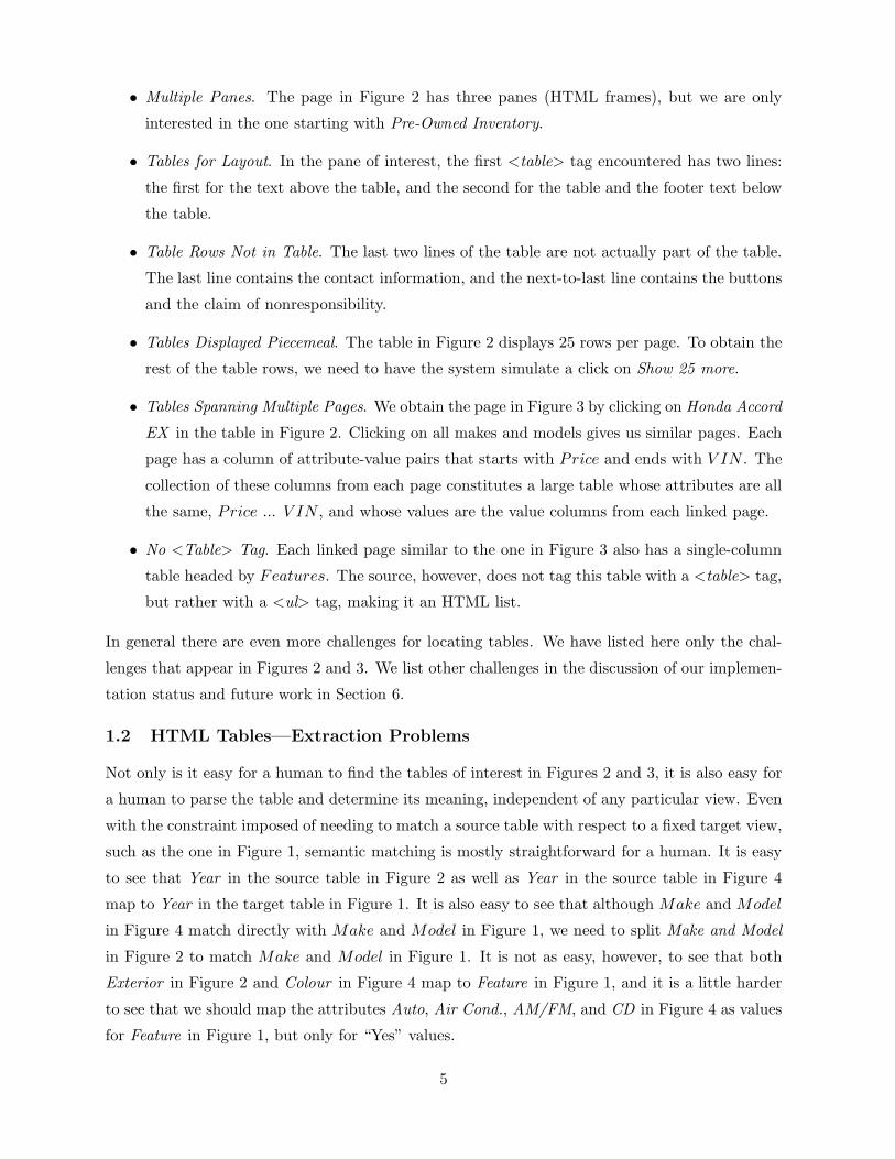
1.1 HTML Tables—Location Problems

It is easy for a human to locate the table of interest in Figure 2. Algorithmically finding the

table of interest on an Web page, however, is often nontrivial, even when the system can tell that

the page is of interest for the given application [ENX01]. Figure 2, for example, presents several

challenges for table location.1The problems encountered in HTML tables are more than sufficient for this investigation. Table extraction

within the broader context of images of paper tables and other types of electronic tables [LN99b] is also possible.

2

Figure 2: Web Page with Table from [Bob03]

3

Figure 3: Linked Page with Additional Information [Bob03]

Figure 4: Table from [Aut01]

4

• Multiple Panes. The page in Figure 2 has three panes (HTML frames), but we are only

interested in the one starting with Pre-Owned Inventory.

• Tables for Layout. In the pane of interest, the first <table> tag encountered has two lines:

the first for the text above the table, and the second for the table and the footer text below

the table.

• Table Rows Not in Table. The last two lines of the table are not actually part of the table.

The last line contains the contact information, and the next-to-last line contains the buttons

and the claim of nonresponsibility.

• Tables Displayed Piecemeal. The table in Figure 2 displays 25 rows per page. To obtain the

rest of the table rows, we need to have the system simulate a click on Show 25 more.

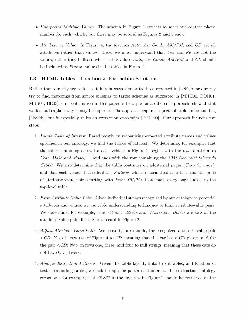
• Tables Spanning Multiple Pages. We obtain the page in Figure 3 by clicking on Honda Accord

EX in the table in Figure 2. Clicking on all makes and models gives us similar pages. Each

page has a column of attribute-value pairs that starts with Price and ends with V IN . The

collection of these columns from each page constitutes a large table whose attributes are all

the same, Price ... V IN , and whose values are the value columns from each linked page.

• No <Table> Tag. Each linked page similar to the one in Figure 3 also has a single-column

table headed by Features. The source, however, does not tag this table with a <table> tag,

but rather with a <ul> tag, making it an HTML list.

In general there are even more challenges for locating tables. We have listed here only the chal-

lenges that appear in Figures 2 and 3. We list other challenges in the discussion of our implemen-

tation status and future work in Section 6.

1.2 HTML Tables—Extraction Problems

Not only is it easy for a human to find the tables of interest in Figures 2 and 3, it is also easy for

a human to parse the table and determine its meaning, independent of any particular view. Even

with the constraint imposed of needing to match a source table with respect to a fixed target view,

such as the one in Figure 1, semantic matching is mostly straightforward for a human. It is easy

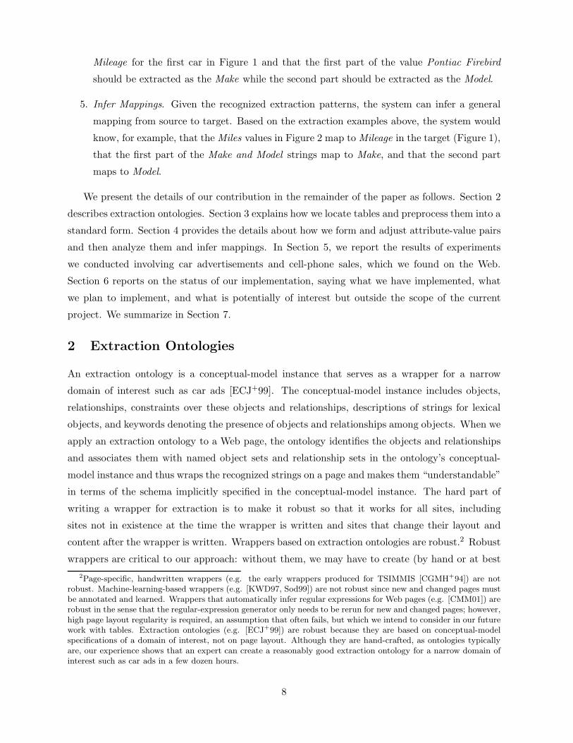
to see that Year in the source table in Figure 2 as well as Year in the source table in Figure 4

map to Year in the target table in Figure 1. It is also easy to see that although Make and Model

in Figure 4 match directly with Make and Model in Figure 1, we need to split Make and Model

in Figure 2 to match Make and Model in Figure 1. It is not as easy, however, to see that both

Exterior in Figure 2 and Colour in Figure 4 map to Feature in Figure 1, and it is a little harder

to see that we should map the attributes Auto, Air Cond., AM/FM, and CD in Figure 4 as values

for Feature in Figure 1, but only for “Yes” values.

5

Algorithmically sorting out these semantic matches is significantly harder. We encounter the

following list the challenges when trying to match source HTML tables in Figures 2, 3, and 4 with

the target schema in Figure 1. We list other challenges in the discussion of our implementation

status and future work in Section 6.

• Merged Attributes/Values. Make and Model are separate attributes in Figure 1 but are

merged as one attribute in Figure 2.

• Subsets. Exterior in Figure 2 and Colour in Figure 4 contain colors. Colors in the target

are a special kind of Feature and thus the sets of colors in Figures 2 and 4 are subsets of the

feature values we want for Figure 1. Indeed, these are proper subsets since there are also

many other feature values in Figures 2, 3, and 4.

• Synonyms. Mileage in Figure 1 and Miles in Figure 2 have the same meaning, but the

attribute names are not the same.

• Extra Information. The tables in Figure 1 make no request for photographs, which are

present in Figure 2.

• Linked Information. The values for the attribute Make and Model are linked to further

information. Clicking on Honda Accord EX in Figure 2 yields the information in Figure 3.

• List Table. A one-dimensional table and a list are similar in appearance. Features in Figure 3

is a list, but could just as easily have been formatted as a table. Although it is a list, we

nevertheless wish to match Features in Figure 3 with Feature in Figure 1.

• Position of Attributes. The linked subtable in Figure 3 has its attributes in the left column,

rather than in the top row.

• Missing Information. The schema in Figure 1 expects a phone number, but none of the

tables in Figures 2, 3, or 4 contains a phone number.

• Externally Factored Data. Although no phone number appears in the tables in Figures 2 or

3, phone numbers do appear in the footer text of the table in Figure 2 and in the text above

the tables in Figure 3. A value, such as a dealer phone number, that applies to all records

in a table is often factored out, external to the table, and displayed only once.

• Duplicate Data. The price for the Honda Accord EX in Figures 2 and 3 appears three times,

once under Price in Figure 2, once as the value for the Price attribute in the (vertical) table

row in Figure 3, and once at the top of the layout table in Figure 3. (Luckily, the values

are all the same.) Other values also appear more than once. The number of miles, in fact,

appears with two different attributes, once with Miles and once with Mileage.

6

• Unexpected Multiple Values. The schema in Figure 1 expects at most one contact phone

number for each vehicle, but there may be several as Figures 2 and 3 show.

• Attribute as Value. In Figure 4, the features Auto, Air Cond., AM/FM, and CD are all

attributes rather than values. Here, we must understand that Yes and No are not the

values; rather they indicate whether the values Auto, Air Cond., AM/FM, and CD should

be included as Feature values in the tables in Figure 1.

1.3 HTML Tables—Location & Extraction Solutions

Rather than directly try to locate tables in ways similar to those reported in [LN99b] or directly

try to find mappings from source schemas to target schemas as suggested in [MHH00, DDH01,

MBR01, BE03], our contribution in this paper is to argue for a different approach, show that it

works, and explain why it may be superior. The approach requires aspects of table understanding

[LN99b], but it especially relies on extraction ontologies [ECJ+99]. Our approach includes five

steps.

1. Locate Table of Interest. Based mostly on recognizing expected attribute names and values

specified in our ontology, we find the tables of interest. We determine, for example, that

the table containing a row for each vehicle in Figure 2 begins with the row of attributes

Year, Make and Model, ... and ends with the row containing the 2001 Chevrolet Silverado

C1500. We also determine that the table continues on additional pages (Show 25 more),

and that each vehicle has subtables, Features which is formatted as a list, and the table

of attribute-value pairs starting with Price $21,988 that spans every page linked to the

top-level table.

2. Form Attribute-Value Pairs. Given individual strings recognized by our ontology as potential

attributes and values, we use table understanding techniques to form attribute-value pairs.

We determine, for example, that <Year : 1999> and <Exterior : Blue> are two of the

attribute-value pairs for the first record in Figure 2.

3. Adjust Attribute-Value Pairs. We convert, for example, the recognized attribute-value pair

<CD : Yes> in row two of Figure 4 to CD, meaning that this car has a CD player, and the

the pair <CD : No> in rows one, three, and four to null strings, meaning that these cars do

not have CD players.

4. Analyze Extraction Patterns. Given the table layout, links to subtables, and location of

text surrounding tables, we look for specific patterns of interest. The extraction ontology

recognizes, for example, that 32,833 in the first row in Figure 2 should be extracted as the

7

Mileage for the first car in Figure 1 and that the first part of the value Pontiac Firebird

should be extracted as the Make while the second part should be extracted as the Model.

5. Infer Mappings. Given the recognized extraction patterns, the system can infer a general

mapping from source to target. Based on the extraction examples above, the system would

know, for example, that the Miles values in Figure 2 map to Mileage in the target (Figure 1),

that the first part of the Make and Model strings map to Make, and that the second part

maps to Model.

We present the details of our contribution in the remainder of the paper as follows. Section 2

describes extraction ontologies. Section 3 explains how we locate tables and preprocess them into a

standard form. Section 4 provides the details about how we form and adjust attribute-value pairs

and then analyze them and infer mappings. In Section 5, we report the results of experiments

we conducted involving car advertisements and cell-phone sales, which we found on the Web.

Section 6 reports on the status of our implementation, saying what we have implemented, what

we plan to implement, and what is potentially of interest but outside the scope of the current

project. We summarize in Section 7.

2 Extraction Ontologies

An extraction ontology is a conceptual-model instance that serves as a wrapper for a narrow

domain of interest such as car ads [ECJ+99]. The conceptual-model instance includes objects,

relationships, constraints over these objects and relationships, descriptions of strings for lexical

objects, and keywords denoting the presence of objects and relationships among objects. When we

apply an extraction ontology to a Web page, the ontology identifies the objects and relationships

and associates them with named object sets and relationship sets in the ontology’s conceptual-

model instance and thus wraps the recognized strings on a page and makes them “understandable”

in terms of the schema implicitly specified in the conceptual-model instance. The hard part of

writing a wrapper for extraction is to make it robust so that it works for all sites, including

sites not in existence at the time the wrapper is written and sites that change their layout and

content after the wrapper is written. Wrappers based on extraction ontologies are robust.2 Robust

wrappers are critical to our approach: without them, we may have to create (by hand or at best2Page-specific, handwritten wrappers (e.g. the early wrappers produced for TSIMMIS [CGMH+94]) are not

robust. Machine-learning-based wrappers (e.g. [KWD97, Sod99]) are not robust since new and changed pages mustbe annotated and learned. Wrappers that automatically infer regular expressions for Web pages (e.g. [CMM01]) arerobust in the sense that the regular-expression generator only needs to be rerun for new and changed pages; however,high page layout regularity is required, an assumption that often fails, but which we intend to consider in our futurework with tables. Extraction ontologies (e.g. [ECJ+99]) are robust because they are based on conceptual-modelspecifications of a domain of interest, not on page layout. Although they are hand-crafted, as ontologies typicallyare, our experience shows that an expert can create a reasonably good extraction ontology for a narrow domain ofinterest such as car ads in a few dozen hours.

8

1. Car [-> object];

2. Car [0:1] has Year [1:*];

3. Car [0:1] has Make [1:*];

4. Car [0:1] has Model [1:*];

5. Car [0:1] has Mileage [1:*];

6. Car [0:*] has Feature [1:*];

7. Car [0:1] has Price [1:*];

8. PhoneNr [1:*] is for Car [0:1];

9. Year matches [4]

10. constant {extract "\d{2}";11. context "\b’[4-9]\d\b";12. substitute "ˆ" -> "19"; },13. ...

14. Mileage matches [8]

15. ...

16. keyword "\bmiles\b", "\bmi\.", "\bmi\b",17. "\bmileage\b", "\bodometer\b";18. ...

Figure 5: Car-Ads Extraction Ontology (Partial)

semiautomatically) a wrapper for every new table encountered; with them, the approach can be

fully automatic.

An extraction ontology consists of two components: (1) an object/relationship-model instance

that describes sets of objects, sets of relationships among objects, and constraints over object and

relationship sets, and (2) for each object set, a data frame that defines the potential contents of

the object set. A data frame for an object set defines the lexical appearance of constant objects

for the object set and establishes appropriate keywords that are likely to appear in a document

when objects in the object set are mentioned. Figure 5 shows part of our car-ads application

ontology, including object and relationship sets and cardinality constraints (Lines 1-8) and a few

lines of the data frames (Lines 9-18).

An object set in an application ontology represents a set of objects which may either be lexical

or nonlexical. Data frames with declarations for constants that can potentially populate the

object set represent lexical object sets, and data frames without constant declarations represent

nonlexical object sets. Year (Line 9) and Mileage (Line 14) are lexical object sets whose character

representations have a maximum length of 4 characters and 8 characters respectively. Make, Model,

Price, Feature, and PhoneNr are the remaining lexical object sets in our car-ads application; Car

is the only nonlexical object set.

We describe the constant lexical objects and the keywords for an object set by regular ex-

pressions using Perl-like syntax.3 When applied to a textual document, the extract clause (e.g.

Line 10) in a data frame causes a string matching a regular expression to be extracted, but only3Thus, for example, “\b” indicates a word boundary, “\d” indicates a numeric digit, and so forth.

9

if the context clause (e.g. Line 11) also matches the string and its surrounding characters. A

substitute clause (e.g. Line 12) lets us alter the extracted string before we store it in an in-

termediate file. (For example, the Year data frame treats a year written “’95” as the constant

“1995”.) We also store the string’s position in the document and its associated object-set name

in the intermediate file. One of the nonlexical object sets must be designated as the object set of

interest—Car for the car-ads ontology, as indicated by the notation “[-> object]” in Line 1.

We denote a relationship set by a name that includes its object-set names (e.g. Car has

Year in Line 2 and PhoneNr is for Car in Line 8). The min:max pairs in the relationship-set

name are participation constraints. Min designates the minimum number of times an object in

the object set can participate in the relationship set and max designates the maximum number

of times an object can participate, with * designating an unknown maximum number of times.

The participation constraint on Car for Car has Feature in Line 6, for example, specifies that a

car need not have any listed features and that there is no specified maximum for the number of

features listed for a car.

In our initial work with semistructured and unstructured Web pages [ECJ+99], a data-extraction

ontology allowed us to recognize data values and context keywords for a particular application,

organize data into records of interest, and fill object and relationship sets with data according

to ontologically specified constraints. In our current work with tables, nested subtables in linked

pages, and surrounding semistructured and unstructured text, we use extraction ontologies in

much the same way. Recognized context keywords tend to be attributes; sometimes recognized

values are also attributes. For tables, geometric layout gives us the clues we need to decide which

recognized strings are attributes and which are values. This knowledge, plus the ontological do-

main knowledge about which attributes and values belong to which object sets, establishes the

basis for determining record groupings and semantic correspondences for target attributes and

relationships. Our system’s ability to extract attributes and values and to pair them together

constitutes the fundamental basis for enabling it to recognize tables containing data of interest

and to discover mapping rules that can transform the contents of source tables to a target schema.

3 Table Location

As a starting place, we assume that we have a Web page with a table whose rows correspond

one-to-one with the fundamental object of interest in our application’s data-extraction ontology.4

We do not assume, however, that we have identified the table on Web page nor that we have, in

hand, any linked pages of interest. The Web page in Figure 2 is an example of such a starting

Web page. The rows in the table of cars in Figure 2 correspond one-to-one with Car, the object

of interest declared in Figure 5.4As stated earlier, we can use previous work [ENX01] to make this determination.

10

Our table-location task is to find the fundamental table of interest in the top-level page and the

tables of interest in linked pages. To resolve the table-location problem, we face all the problems

mentioned in the introduction, i.e., Multiple Panes, Tables for Layout, Table Rows Not in Table,

Tables Displayed Piecemeal, Tables Spanning Multiple Pages, and No <Table> Tag. We also face

other problems we have encountered, including some that our system handles, such as folded

tables and factored rows, and some that we report as future challenges in Section 6.

Our system resolves the problems of finding the main table of interest by using the following

heuristics.

• Potential Table. The main table must be embedded in an HTML <Table>.

• Table Size. The main table must have at least three rows and at least three columns.

• Grid Layout. We can count the number of data cells in each row in the table. Letting N be

the number of rows in the table that have the most common number of data cells and M

be the number of rows in the table, the ratio N/M must exceed 2/3. This ensures that the

vast majority of the rows extend across the width of the table and thus that the table, at

least roughly, has the expected geometry of a table.

• Attributes. Based on the keywords and the object-set names for the various object sets in

our extraction ontology, we have a reasonable idea about what some of the attribute names

for a table should be. Thus, we look for a row near the top from which we have been able to

extract 60% of the data entries as attributes—these attributes, of course, must be distinct.

(Note that we do not depend on the table creator to mark the attributes with a <th> tag.)

If we cannot find an attribute row in the table, we try columns, preferably leftmost columns.

If we find an attribute column, we can transpose the table so that the attributes are in rows.

• Value Density. Based on the values expected for the various lexical object sets, we find all

ontology-recognized strings. If the ratio of the number of characters in recognized strings

to the total number of characters in strings within the table exceeds 10%, we have some

reasonable evidence that the table is of interest for the application. (Although 10% may

seem low, previous experiments with density [EJN99] show that the density test should fail

only for extremely low percentages, usually below 1%.)

• Folded Tables. Sometimes tables have so many columns that table designers fold them for

viewing on a single page or in a single window either by placing the second half of the

columns below the first half of the columns or by making two (or more) rows of attributes at

the top that associate with pairs (triples, ...) of values in the columns below. Thus, if more

than one attribute row appears, we compare the attribute rows. If they are not the same,

we treat the table as a folded table; otherwise we remove the duplicate attribute rows.

11

• Factored-Value Rows. We consider as possible factored values those values in each table row

where the row has less than half the cells filled and the cells that are filled are adjacent

left-most fields. (Many car-ads tables, for example, group cars by year and display the

year in a row by itself above all the cars listed for that year.) We add factored values that

are above the attribute row to all subsequent rows, and we add factored values that are

below the attribute row to all subsequent rows until the next row of factored values. We

eliminate rows that do not satisfy these factoring criteria—presumable these are not value

table rows—for example, the row of buttons at the bottom of the table in Figure 2.

• “More”-Link Pages. We can make use of linked components of the top-level table to help

determine with certainty which strings are attributes and which are values by observing

that the attributes remain the same across pages while the values change. For the page

in Figure 2, for example, all subsequent pages linked by “Show 25 more” have identical

attributes on the top row of the table, namely

Year, Make and Model, Price, Miles, Exterior, Photo.

Indeed, in this way, we are likely to be able to identify attributes, such as Photo, even when

they are not in our application ontology.

For tables in linked pages, table detection is different. We use the following heuristics for these

tables.

• Table Size. We do not expect subtables to be as large as top-level tables. Thus we only

require at least two rows or two columns.

• Attributes. This is the same as for top-level tables.

• Attribute-Value-Pair Table To locate table components that contain attribute-value pairs,

we look for a pair of columns where the strings in the first column have been extracted

mostly as attributes and the strings in the second column have been extracted mostly as

values. The table component in Figure 3 is an example—the left column starting with Price

contains many strings our extraction ontology recognizes as attributes, and the right column

starting with $21,988 contains many strings our extraction ontology recognizes as values.

Sometimes these types of tables are folded, so we must consider several pairs of columns

side by side. As for other attribute tests, we use 60% as our threshold. We also check for

row pairs in the same way to locate table components formatted with the attributes above

the values, rather than to the left.

12

• Single-Attribute Table. To find lists like the Features list in Figure 3, we look for a <ul> or

an <ol> tag or for a <table> tag followed by a single-column table structure. We confirm

that the single-attribute table is of interest by checking whether the ontology recognizes at

least 60% of the strings as values of interest.

• Page-Spanning Tables. We follow a selected number of links from the top-level table to

obtain several linked table rows. We then check the variability—attributes tend to remain

the same from page to page (although sometimes table rows have more or fewer attributes),

while values tend to vary (although some, such as colors, body styles, and transmission types

are often identical).

4 Derivation of Source-to-Target Schema Mappings

We assume that each tuple in the top-level table corresponds to a primary object of interest.5 One

consequence of this assumption is that we can simply generate an object identifier for each of these

objects. Indeed, this is how we obtain the values under the attribute Car in Figure 1. Another

consequence of this assumption is that we can easily group the source information into record

chunks, one chunk of information for each object of interest. The information chunk for the 2002

Honda Accord EX in Figure 2, for example, is the third tuple in the table plus all the information

in Figure 3. Having record chunks allows us to more easily build the atomic relationships between

an object of interest and its associated data once we find the semantic correspondence for each

target attribute. Hence, we are able to reduce the problem of finding a semantic correspondence

to just finding the semantic correspondence for each target attribute A, which we defined earlier

as the problem of finding the set of values constructed from source elements that corresponds to

A.

We accomplish this objective using a “back-door” approach. Instead of directly searching for a

mapping that associates each target attribute A with a value set in a source, we use our extraction

ontology to search for values in the source that are likely to be found in the value set for A. Then,

from the pattern of values we find, we infer what the mapping must be. This approach more

easily allows us to recognize some of the unusual indirect mappings we are likely to encounter

such as Attribute as Value, Externally Factored Data, and Merged Attributes/Values as discussed

and illustrated in the introduction. The following four subsections correspond to the four steps of

our proposed approach that follow the step of locating the table of interest, discussed previously

in Section 3.5We do not address fundamental mismatches of primary objects in our work here. Whether this approach extends

to cases where we cannot easily find an alignment for the main objects of interest (cars in our example here) is aquestion for future research.

13

4.1 Form Attribute-Value Pairs

The table understanding problem takes as input a table (for our work here, an HTML table) and

produces standard records as output. Each record produced is a set of attribute-value pairs. A

successful table-understanding system, for example, would produce the first record in the table in

Figure 4 as

{<Make: ACURA>, <Model : legend>, <Year : 1992>, <Colour : grey>,

<Price: $9500>, <Auto: Yes>, <Air Cond.: No>, <AM/FM : Yes>, <CD : No>}

The hard part of table understanding is to recognize which cells contain the attributes and

which contain the values and then to recognize which attributes go with which values. Our table

recognition heuristics help solve this problem, at least for top-level tables whose attributes are

at the top of columns and for linked subtables, which may be tables in their own right, simple

one-column lists, or table-row components of tables that span multiple pages.6

Once we have identified attributes, we can immediately associate each cell in the grid layout

of a table with its attribute. If the cell is not empty, we also immediately have a value for the

attribute and thus an attribute-value pair. If the cell is empty, however, we must infer whether

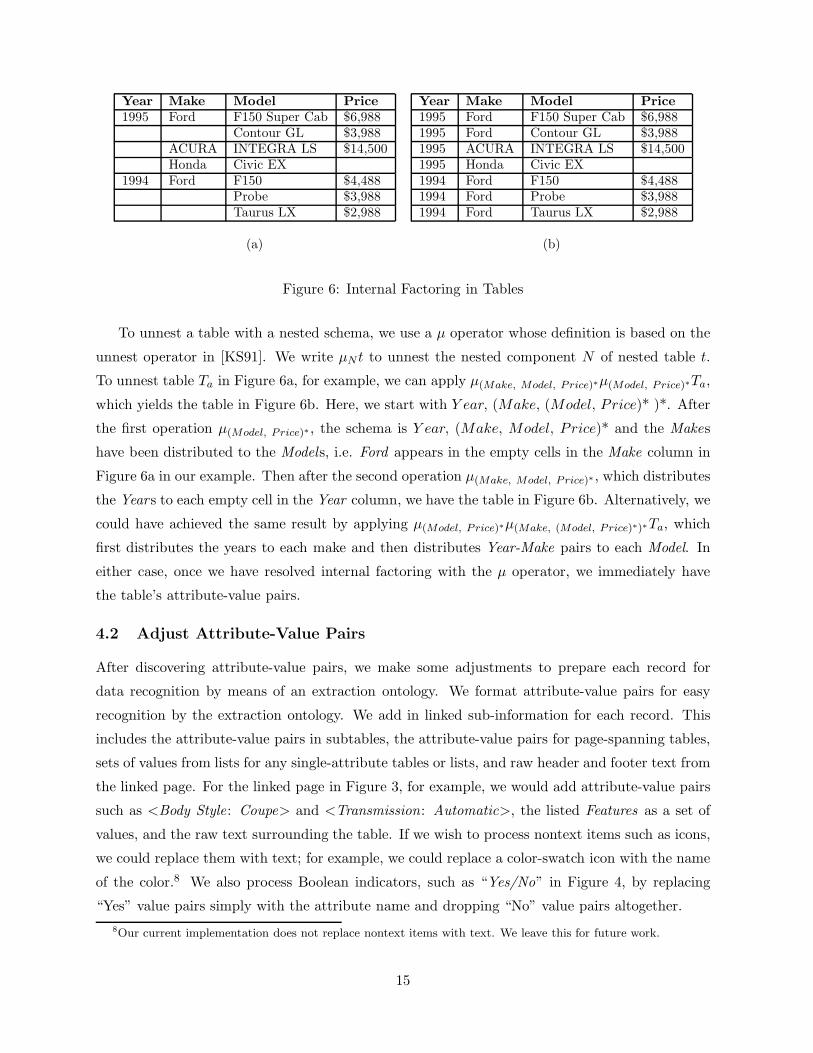
the table has a value based on internal factoring or whether there is no value. Figure 6a shows an

example of internal factoring. The empty Year cell for the Contour GL, for example, is clearly

1995, whereas the Price for the Honda is simply missing. We recognize internal factoring in a

two-step process:7 (1) we detect potential factoring by observing a pattern of empty cells in a

column, preferably a leftmost column or a near-leftmost column; (2) we check to see whether

adding in the value above the empty cell helps complete a record by adding a value that would

otherwise be missing.

Once we recognize the factoring in a table, we can rewrite the table’s schema as a nested

schema that reflects the factoring and then unnest the table to distribute factored values and to

return the schema for the nested table to an unnested schema. Textually, we represent a nested

component of a schema by (Ai, ..., An)* where the Ai’s are attribute names. In general, nested

components may appear inside of and along side of other nested components. The nested schema

that defines the internal factoring for the table in Figure 6a is Y ear, (Make, (Model, Price)* )*.6We recognize that [LN99a] had an earlier solution for a much smaller subclass of HTML tables. We also recognize

that there is a larger class of HTML tables and an even larger class of tables in general [LN99b]. In our work here,however, we accept this intermediate, simpler solution for now, but in some of our other work [Haa98, Tub01] wehave explored the attribute-recognition problem for a larger class of tables, and in future work, we intend to providea solution to finding attribute-value pairs in general tables. Once we or others have a general solution, the approachwe propose here carries over without change.

7This procedure is more fully described in [EX00], where we explain how we use a multi-dimensional cosinemeasure and a hill-climbing procedure to recognize factored values and appropriately distribute them to theirproper records.

14

Year Make Model Price Year Make Model Price1995 Ford F150 Super Cab $6,988 1995 Ford F150 Super Cab $6,988

Contour GL $3,988 1995 Ford Contour GL $3,988ACURA INTEGRA LS $14,500 1995 ACURA INTEGRA LS $14,500Honda Civic EX 1995 Honda Civic EX

1994 Ford F150 $4,488 1994 Ford F150 $4,488Probe $3,988 1994 Ford Probe $3,988Taurus LX $2,988 1994 Ford Taurus LX $2,988

(a) (b)

Figure 6: Internal Factoring in Tables

To unnest a table with a nested schema, we use a µ operator whose definition is based on the

unnest operator in [KS91]. We write µN t to unnest the nested component N of nested table t.

To unnest table Ta in Figure 6a, for example, we can apply µ(Make, Model, P rice)∗µ(Model, P rice)∗Ta,

which yields the table in Figure 6b. Here, we start with Y ear, (Make, (Model, Price)* )*. After

the first operation µ(Model, P rice)∗, the schema is Y ear, (Make, Model, Price)* and the Makes

have been distributed to the Models, i.e. Ford appears in the empty cells in the Make column in

Figure 6a in our example. Then after the second operation µ(Make, Model, P rice)∗, which distributes

the Years to each empty cell in the Year column, we have the table in Figure 6b. Alternatively, we

could have achieved the same result by applying µ(Model, P rice)∗µ(Make, (Model, P rice)∗)∗Ta, which

first distributes the years to each make and then distributes Year-Make pairs to each Model. In

either case, once we have resolved internal factoring with the µ operator, we immediately have

the table’s attribute-value pairs.

4.2 Adjust Attribute-Value Pairs

After discovering attribute-value pairs, we make some adjustments to prepare each record for

data recognition by means of an extraction ontology. We format attribute-value pairs for easy

recognition by the extraction ontology. We add in linked sub-information for each record. This

includes the attribute-value pairs in subtables, the attribute-value pairs for page-spanning tables,

sets of values from lists for any single-attribute tables or lists, and raw header and footer text from

the linked page. For the linked page in Figure 3, for example, we would add attribute-value pairs

such as <Body Style: Coupe> and <Transmission: Automatic>, the listed Features as a set of

values, and the raw text surrounding the table. If we wish to process nontext items such as icons,

we could replace them with text; for example, we could replace a color-swatch icon with the name

of the color.8 We also process Boolean indicators, such as “Yes/No” in Figure 4, by replacing

“Yes” value pairs simply with the attribute name and dropping “No” value pairs altogether.8Our current implementation does not replace nontext items with text. We leave this for future work.

15

Make Model Year Colour Price Auto Air Cond. AM/FM CDACURA legend 1992 grey $9500 Auto AM/FMAUDI A4 2000 Blue $34,500 Auto Air Cond. AM/FM CDBMW 325e 1985 black $2700.00 AM/FMCHEVROLET Cavalier Z24 1997 Black $11,995.00 Air Cond. AM/FM

Figure 7: Table in Figure 4 Transformed by the β Operator

For our running example, the adjusted attribute-value pairs in the first record in Figure 4

become

Make: ACURA; Model : legend ; Year : 1992; Colour : grey ; Price: $9500; Auto; AM/FM ;

Note that the Boolean-valued attribute-value pairs <Auto: Yes> and <AM/FM : Yes> have

become simply Auto, meaning that the car has an automatic transmission, and AM/FM, meaning

that the car has an AM/FM radio, and that Air Cond. and CD have disappeared altogether,

meaning that the car has neither air conditioning nor a CD player.

When attribute names are the values we want and the values are some sort of Boolean indicator

(e.g. Yes/No, True/False, 1/0, cell checked or empty), we transform the Boolean indicators into

attribute-name values with the help of a β operator which we introduce here. Syntactically we

write βAT,F r where A is an attribute of relation r and T and F are respectively the Boolean

indicators for the True value and the False value given as A values in r. The result of the β

operator is r with the True values of the A column replaced by the string A and the False values

of A replaced by the null string. As an example, consider βAutoY es,Noβ

Air Cond.Y es,No β

AM/FMY es,No βCD

Y es,NoT

which transforms the table T in Figure 4 to the table in Figure 7.

4.3 Perform Extraction

Once we have adjusted attribute-value pairs as just discussed, we apply our extraction ontology.

For our running example, the extraction for the first record in Figure 4 yields

{<Car : 0011>, <Year : 1992>, <Make: ACURA>, <Model : legend>, <Mileage: >,

<Price: $9500>, <PhoneNr : >},{<Car : 0011>, <Feature: grey>},{<Car : 0011>, <Feature: Auto>},{<Car : 0011>, <Feature: AM/FM>}.

We emphasize that our extraction ontology is capable of extracting from unstructured text as well

as from structured text. Indeed, we can directly extract the phone numbers and features from the

text, list, and page-spanning table in Figure 3.

16

For direct extraction we introduce the ε operator, which is based on a given extraction ontology.

We define εSt as an operator that extracts a value, or values, from unstructured or semistructured

text t for object set S in the given extraction ontology O according to the extraction expression for

S in O. The ε operator extracts a single value if S functionally depends on the object of interest

x in O, and it extracts multiple values if S does not functionally depend on x. As an example,

εPhoneNrt extracts 1-877-944-2842 from the unstructured footer text t of the table in Figure 2 and

returns it as the single-attribute, single-tuple, constant relation {<PhoneNr : 1-877-944-2842>}.We can use the ε operator in conjunction with a natural join to add a column of constant values

to a table. For example, letting t represent the unstructured text on the page in Figure 2 we could

apply εPhoneNrt � T to add a column for PhoneNr to table T in Figure 2.

At this point we could take a data-warehousing approach and directly insert this extracted

information into a global database as Figure 1 implies. Alternatively, instead of populating the

global database, we can use this information to infer a mapping from the source to the target

and extract information from sources whenever a user poses a query against the global database

schema.

4.4 Infer Mappings

We record the sequence of transformations produced when we form attribute-value pairs and when

we adjust attribute-value pairs in preparation for extraction, and we observe the correspondence

patterns obtained when we extract tuples with respect to a given target ontology. Based on this

sequence of transformations and these correspondence patterns, we can produce a mapping of

source information to a target ontology. As a simple example, consider mapping the table Ta in

Figure 6a to the target schema for the tables in Figure 1. We first apply the µ operator to do the

unnesting and obtain table Tb in Figure 6b. We then observe that objects extracted for the Year

object set in the target come from the Year column in Tb. Similarly, for Make, Model, and Price,

we also observe a direct correspondence. Hence, we can record the semantic correspondence of Ta

and the target schema as the mapping Year = πY earµ(Make, Model, P rice)∗µ(Model, P rice)∗Ta, Make

= πMakeµ(Model, P rice)∗Ta, Model = πModelTa, and Price = πPriceTa.

Creating an inferred mapping has two important advantages. (1) The global view can be

virtual. Since we have a formal mapping, we can translate any query applied to the global view

to a query on the source, optimize it, execute it, and return the results from the source for the

global query.9 (2) We can obtain additional values not recognized by the ontology, but which are9Since the main contribution of this paper is the derivation of the mappings, not local query rewriting [LRO96,

Ull97], we leave for future research a full explanation of this procedure. The idea, however, is quite straightforwardonce we have the semantic correspondence. Since we know the record structure of the source, we can add objectidentifiers for each value in the value sets. We can then join over these OID-augmented value sets to obtain auniversal relation. Since the mappings result in sets associated with target attributes, if we add columns of nullsfor each target attribute with no correspondence, we will have a universal relation over the target attributes. We

17

nevertheless valid values in the source. For example, Super Cab may not be technically part of

the model for the 1995 Ford F150 in Figure 6a, and the ontology may therefore not recognize it

as part of the model. Nevertheless, someone declared Super Cab to be part of the model, and

we should therefore extract it as such. Using the mapping, we extract full strings under Model

in Figure 6a and thus we obtain F150 Super Cab as the model for the 1995 Ford even though

the extraction ontology may only pick up F150 as the model. As another example, the mapping

approach would obtain all the Features in the list in Figure 3 even though the ontology may not

recognize all of them as features. When we use the mapping, we generalize over the structure and

infer additional information not specifically recognized by the ontology.10

To complete our task, we now define a few more operators. These operators, together with the

ones we defined earlier, provide the complete set of operators we need for mapping all the HTML

tables we have encountered.11

For merged attributes we need to split values. We can divide values into smaller components

with a δ operator which we introduce here. We define δAB1,...,Bn

r to mean that each value v for

attribute A of relation r is split into v1, ..., vn, one for each new attribute B1, ..., Bn respectively.

Associated with each Bi is a procedure pi that defines which part of v becomes vi. In this

paper we specify each procedure pi by regular expressions with extract and context phrases

similar to those defined for extraction ontologies discussed earlier in Section 2. The result of the

δ operator is r with n new attributes, B1, ..., Bn, where the Bi value on row k is the string

that results from applying pi to the string v on row k for attribute A. As an example, consider

δMake and ModelMake,Model T , where T is the table in Figure 2, the expression associated with Make is extract

"\S+" context "\S+\s" which extracts the characters of the string value up to the first space,

and the expression associated with Model is extract "\S.*" context "\s.+" which extracts all

the remaining characters in the string after the first space.12 This operation adds the two columns

in Figure 8 to the table in Figure 2.

For split attributes we need to merge values. We can gather values together and merge them

with a γ operator which we introduce here. Syntactically, we write γB ← A1+...+Anr where B is a

new attribute of the relation r and each Ai is either an attribute of r or is a string. The result

of the γ operator is r with an additional attribute B, where the B value on row k is a sequential

concatenation of the row-k values for the attributes along with any given strings. As an example,

can now project onto the schema for each of the target tables. We thus have a standard view definition, which wecan substitute for each of the table references in a global query. We can then optimize the query and execute it onthe source, returning only those values from the source that contribute to the global query result.

10For future research, we are considering the possibility of strengthening recognizers for extraction ontologiesas they encounter additional values recognized through mappings, but not recognized directly through regularexpressions. Strengthening ontologies in this way is similar to the work on learning reported in [JMNR99, RJ99].

11In future research, we would like to obtain a general completeness result.12In Perl, “\s” matches a white space character, “\S” matches a non-space character, “.” matches any character,

“+” indicates one or more repetitions, and “*” indicates zero or more repetitions.

18

Make ModelPontiac FirebirdAcura RL 3.5Honda Accord EXHonda Passport

...Honda Accord Value PackageChevrolet Silverado C1500

Figure 8: Columns Added to the Table in Figure 2 by the δ Operator

T1 Make Model Trim T2 Make Model Trim Model with TrimFord Contour GL Ford Contour GL Contour GLFord Taurus LX Ford Taurus LX Taurus LXHonda Civic EX Honda Civic EX Civic EX

Figure 9: Application of the γ Operator to Table T1 Yielding Table T2

consider γModel with Trim ← Model+" "+TrimT1 which converts Table T1 in Figure 9 to Table T2.

We can use standard set operators to help sort out subsets, supersets, and overlaps of value sets.

We can, for example, take a union of the exterior colors in Figure 2 and features in Figure 3 to form

part of the set for Feature in Figure 1. After adding needed projection and renaming operations,

this union is ρExterior ← FeatureπExteriorT ∪ ρFeatures ← FeatureT/Make and Model/Features, where

T is the table in Figure 2 and T/Make and Model/Features is a path expression that follows the

link under Make and Model in table T to the Features list in Figure 3. When we need subsets of

a set, we can extend the standard selection operator σCr to allow C to be a regular expression

that identifies the subset of values we wish to include. Given that we can also apply set-difference

operations, we can resolve overlapping sets by operator combinations.

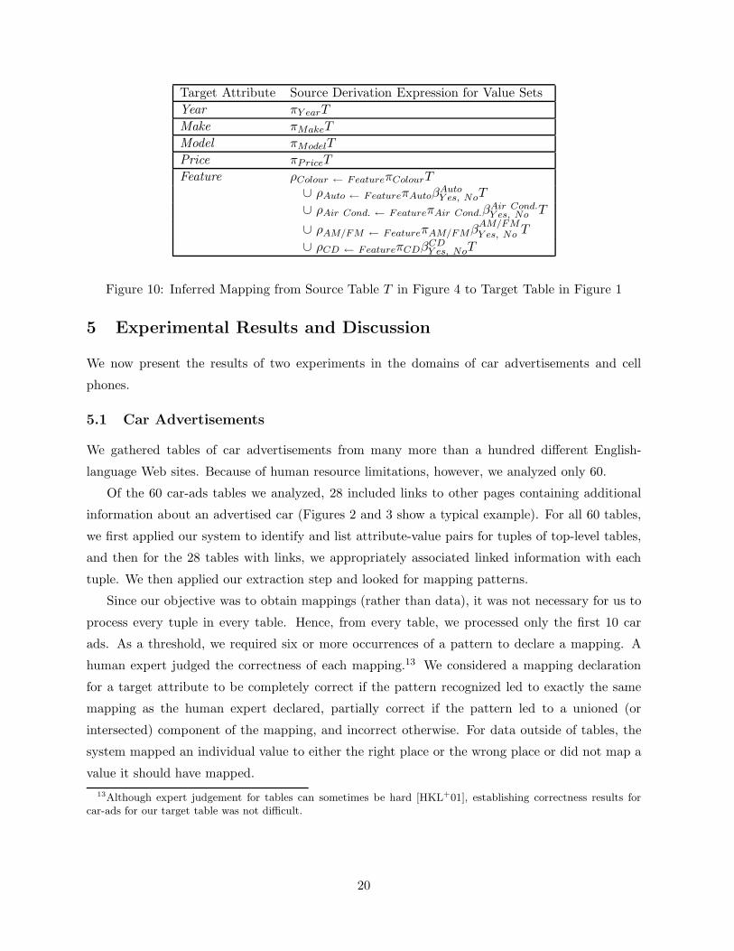
Now that we have the operators we need, we can give examples. Figure 10 gives the mapping

from the source table in Figure 4 to the target table in Figure 1. Observe that we have transformed

all the Boolean values into attribute-name values and that we have gathered together all the

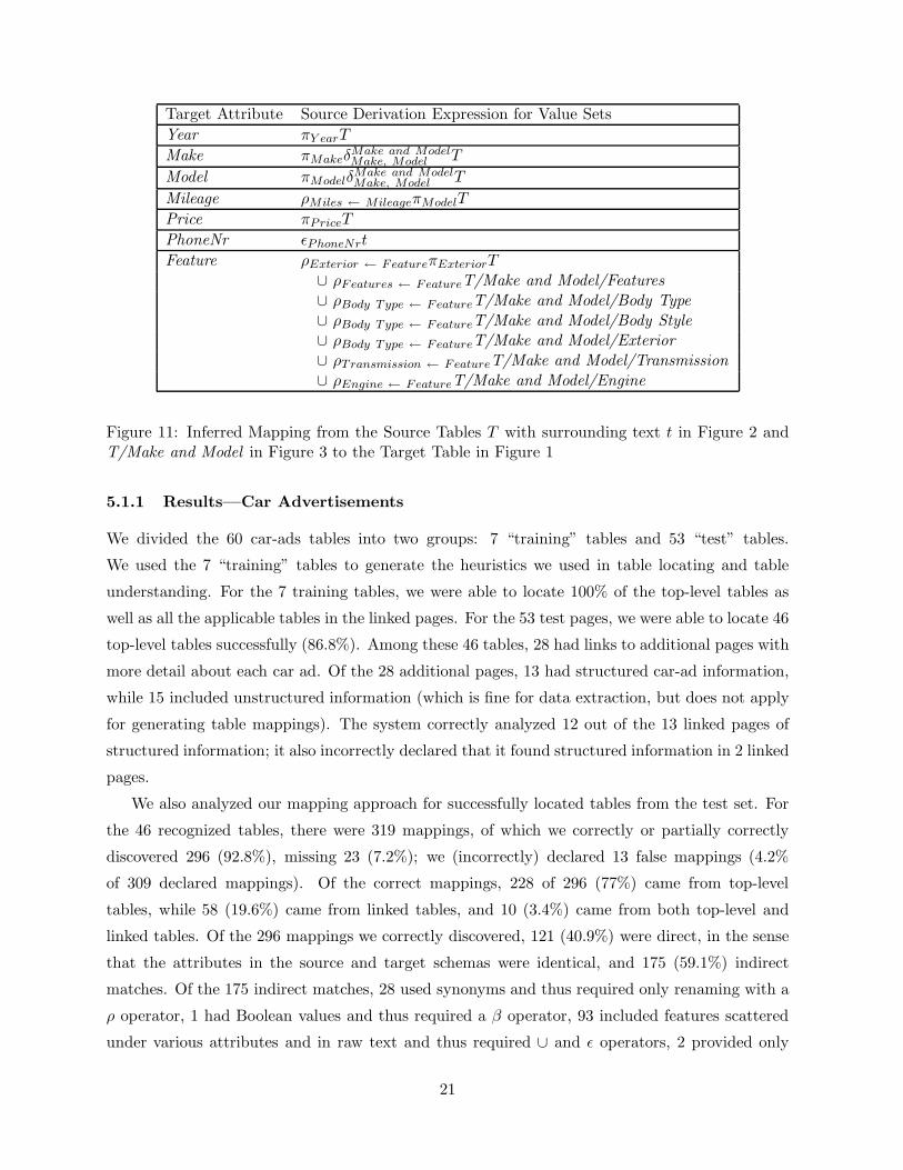
features as Feature values. Figure 11 gives the mapping for the car ads from the site for Figures 2

and 3. Observe that we have split the makes and models as required, matched the synonyms

Miles and Mileage, extracted the PhoneNr from the free text, and gathered together all the

various features as Feature values. The astute reader will have noticed that we extracted only

one Price and Mileage even though two or more appear—since they functionally depend on car,

we pick up only the first—and that we union in the color twice—once from the top-level table

in Figure 2 and once from the page-spanning table in Figure 3 since Feature does not depend

functionally on car. The astute reader will have also noticed that we did not pick up the Fuel

Type, Stock Number, and VIN—these, like Photo, neither appear separately in our ontology nor

as recognized features in our ontology.

19

Target Attribute Source Derivation Expression for Value SetsYear πY earT

Make πMakeT

Model πModelT

Price πPriceT

Feature ρColour ← FeatureπColourT∪ ρAuto ← FeatureπAutoβ

AutoY es, NoT

∪ ρAir Cond. ← FeatureπAir Cond.βAir Cond.Y es, No T

∪ ρAM/FM ← FeatureπAM/FMβAM/FMY es, No T

∪ ρCD ← FeatureπCDβCDY es, NoT

Figure 10: Inferred Mapping from Source Table T in Figure 4 to Target Table in Figure 1

5 Experimental Results and Discussion

We now present the results of two experiments in the domains of car advertisements and cell

phones.

5.1 Car Advertisements

We gathered tables of car advertisements from many more than a hundred different English-

language Web sites. Because of human resource limitations, however, we analyzed only 60.

Of the 60 car-ads tables we analyzed, 28 included links to other pages containing additional

information about an advertised car (Figures 2 and 3 show a typical example). For all 60 tables,

we first applied our system to identify and list attribute-value pairs for tuples of top-level tables,

and then for the 28 tables with links, we appropriately associated linked information with each

tuple. We then applied our extraction step and looked for mapping patterns.

Since our objective was to obtain mappings (rather than data), it was not necessary for us to

process every tuple in every table. Hence, from every table, we processed only the first 10 car

ads. As a threshold, we required six or more occurrences of a pattern to declare a mapping. A

human expert judged the correctness of each mapping.13 We considered a mapping declaration

for a target attribute to be completely correct if the pattern recognized led to exactly the same

mapping as the human expert declared, partially correct if the pattern led to a unioned (or

intersected) component of the mapping, and incorrect otherwise. For data outside of tables, the

system mapped an individual value to either the right place or the wrong place or did not map a

value it should have mapped.13Although expert judgement for tables can sometimes be hard [HKL+01], establishing correctness results for

car-ads for our target table was not difficult.

20

Target Attribute Source Derivation Expression for Value SetsYear πY earT

Make πMakeδMake and ModelMake, Model T

Model πModelδMake and ModelMake, Model T

Mileage ρMiles ← MileageπModelT

Price πPriceT

PhoneNr εPhoneNrt

Feature ρExterior ← FeatureπExteriorT∪ ρFeatures ← FeatureT/Make and Model/Features∪ ρBody Type ← FeatureT/Make and Model/Body Type∪ ρBody Type ← FeatureT/Make and Model/Body Style∪ ρBody Type ← FeatureT/Make and Model/Exterior∪ ρTransmission ← FeatureT/Make and Model/Transmission∪ ρEngine ← FeatureT/Make and Model/Engine

Figure 11: Inferred Mapping from the Source Tables T with surrounding text t in Figure 2 andT/Make and Model in Figure 3 to the Target Table in Figure 1

5.1.1 Results—Car Advertisements

We divided the 60 car-ads tables into two groups: 7 “training” tables and 53 “test” tables.

We used the 7 “training” tables to generate the heuristics we used in table locating and table

understanding. For the 7 training tables, we were able to locate 100% of the top-level tables as

well as all the applicable tables in the linked pages. For the 53 test pages, we were able to locate 46

top-level tables successfully (86.8%). Among these 46 tables, 28 had links to additional pages with

more detail about each car ad. Of the 28 additional pages, 13 had structured car-ad information,

while 15 included unstructured information (which is fine for data extraction, but does not apply

for generating table mappings). The system correctly analyzed 12 out of the 13 linked pages of

structured information; it also incorrectly declared that it found structured information in 2 linked

pages.

We also analyzed our mapping approach for successfully located tables from the test set. For

the 46 recognized tables, there were 319 mappings, of which we correctly or partially correctly

discovered 296 (92.8%), missing 23 (7.2%); we (incorrectly) declared 13 false mappings (4.2%

of 309 declared mappings). Of the correct mappings, 228 of 296 (77%) came from top-level

tables, while 58 (19.6%) came from linked tables, and 10 (3.4%) came from both top-level and

linked tables. Of the 296 mappings we correctly discovered, 121 (40.9%) were direct, in the sense

that the attributes in the source and target schemas were identical, and 175 (59.1%) indirect

matches. Of the 175 indirect matches, 28 used synonyms and thus required only renaming with a

ρ operator, 1 had Boolean values and thus required a β operator, 93 included features scattered

under various attributes and in raw text and thus required ∪ and ε operators, 2 provided only

21

factored telephone numbers and thus required ε and � operators, 53 needed to be split and thus

required a δ operator, and some required combinations of these operators (e.g. synonyms and

union). The values we needed to split came in a variety of different combinations and under a

variety of different names. We found, for example, Description as an attribute for the combination

Year+Make+Model+Feature, Model Color as an attribute for Make+Model+Color, and Model

as an attribute for Year+Make+Model.

5.1.2 Discussion—Car Advertisements

Locating the correct table and understanding it properly is not a trivial problem. As we discussed

in Section 3, we consider attributes, values, and table layout when seeking a table. Our system

failed to locate 7 out of 53 test tables. All but one of the 7 missed tables contained uncommon

attributes in the source page. For example, some Web sites use abbreviations like “PW”, “PL”,

“CC”, and “AC”; others include attributes that are irrelevant to the extraction ontology, such

as “Image”, “Click on Thumbnail”, and “Location”. This caused our system to fail to detect

an attribute row (or column) in a table, leading to a failure to identify the correct table. The

other table-location failure occurred because the top table only had 2 columns, but we required a

minimum size of 3 columns by 3 rows.

For linked pages, the system was not able to find the correct table (single attribute-value pairs)

for one site (out of 13). This is because all cars shared a single linked page containing information

for all the cars (a case we had not considered). Our system incorrectly identified two linked pages

as containing tables of interest because it interpreted some values as attributes or vice versa.

As mentioned in our earlier discussion, discovering correct mappings can lead to an increase

in values extracted compared to what would have been found by the extraction ontology alone

and can also therefore lead to the acquisition of additional knowledge for the extraction ontology.

In our experiments, we required 60% of the values to match to declare a mapping. Overall,

we actually achieved roughly 90–95%, a much higher percentage. This, however, leaves about

5–10% of the approximately 3,000 values encountered in tables as being unrecognized by the

extraction ontology (and potentially many hundreds more since we processed only 10 car ads per

site). Examples include non-U.S. models such as the Toyota Starlet or Nissan Presea; elaborately

described features such as “telescoping steering wheel”; abbreviations not encountered previously

such as “leath int” for “leather interior”; and features simply not encountered before, such as

“trip computer”.

We missed 23 mappings and only declared 13 false mappings. Our system missed 10 mappings

of car model because the extraction ontology was targeted to U.S. car ads, and so non-U.S. car

ads introduced models that our system did not recognize. The system missed 2 price mappings, 1

mileage mapping, and 2 feature mappings because the extraction ontology was overly restrictive.

22

All of these problems can be corrected by minor adjustments to the extraction ontology. The

system missed another 5 mappings because of bugs in the original documents (ill-formed HTML)

or due to the use of special codes to indicate particular values like colors. Sometimes Web sites use

generic “filler” values such as “contact us,” “please call,” or “unknown” instead of listing actual

prices, mileages, and so on; we missed 3 mappings for this reason. For the 13 incorrect mappings,

8 came from incorrectly understood linked pages. One of these 8, for example, maps “Location”

to “Model,” because the location is “Aurora” (a city in Colorado) which is also a model name for

Oldsmobile. The other primary confusion for our tool was distinguishing between numbers such

as price and mileage.

5.2 Cell-Phone Sales

The car-advertisements example uses our most mature extraction ontology, and so we expected

to achieve good results using it. To see how our table understanding approach works with less

developed extraction ontologies, we tested our system in the U.S. cell-phone sales domain. Fig-

ure 12 shows part of a top page of a typical cellular-phone application, and Figure 13 shows part

of a page obtained by clicking on Mlife Local $29.99. We used the following target schema:

{Plan, Carrier, MonthlyFee, AnyTimeMin, OffPeakMin, ContractLength,

ActivationFee CancellationFee }{Plan, Feature}.

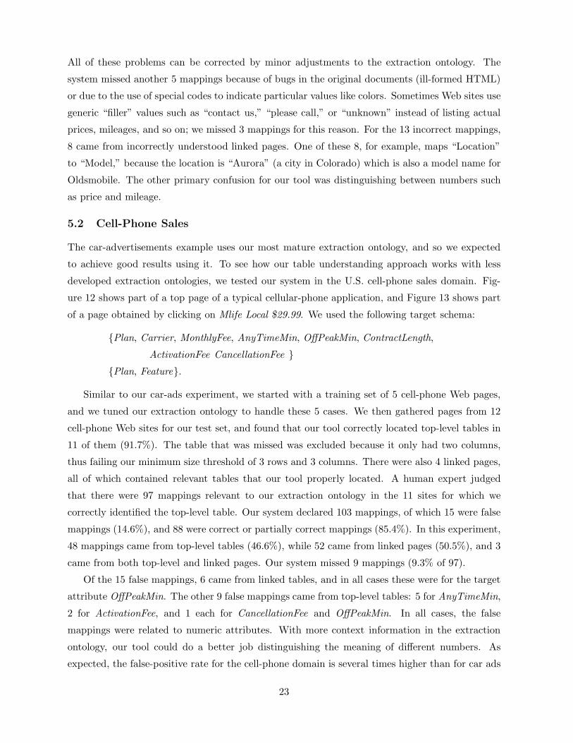
Similar to our car-ads experiment, we started with a training set of 5 cell-phone Web pages,

and we tuned our extraction ontology to handle these 5 cases. We then gathered pages from 12

cell-phone Web sites for our test set, and found that our tool correctly located top-level tables in

11 of them (91.7%). The table that was missed was excluded because it only had two columns,

thus failing our minimum size threshold of 3 rows and 3 columns. There were also 4 linked pages,

all of which contained relevant tables that our tool properly located. A human expert judged

that there were 97 mappings relevant to our extraction ontology in the 11 sites for which we

correctly identified the top-level table. Our system declared 103 mappings, of which 15 were false

mappings (14.6%), and 88 were correct or partially correct mappings (85.4%). In this experiment,

48 mappings came from top-level tables (46.6%), while 52 came from linked pages (50.5%), and 3

came from both top-level and linked pages. Our system missed 9 mappings (9.3% of 97).

Of the 15 false mappings, 6 came from linked tables, and in all cases these were for the target

attribute OffPeakMin. The other 9 false mappings came from top-level tables: 5 for AnyTimeMin,

2 for ActivationFee, and 1 each for CancellationFee and OffPeakMin. In all cases, the false

mappings were related to numeric attributes. With more context information in the extraction

ontology, our tool could do a better job distinguishing the meaning of different numbers. As

expected, the false-positive rate for the cell-phone domain is several times higher than for car ads

23

Figure 12: Web Page with Table of Cell Phones from Buy.com

(14.6% versus 4.2%), which can be attributed partially to the relative amount of effort spent in

developing the corresponding extraction ontologies, and partially to the high degree of similarity

between the domains of attributes in the cell-phone application.

An interesting aspect of the cell-phone domain is that of the 88 mappings we correctly dis-

covered, none were direct (as compared to 40.9% for car ads). That is, we had to apply some

transformation operator to every mapping in the cell-phone application: 38 mappings used syn-

onyms and thus required a ρ operator for renaming; 34 mappings included features scattered under

various attributes, and thus required ∪ operators; and 24 mappings needed to be split and thus

required a δ operator. Some mappings required combinations of operators.

The overall performance of our tool in the cell-phone sales domain is reasonably good and

generally in line with our expectations. We could improve the outcome by tuning the extraction

ontology more carefully.

24

Figure 13: Linked Page with Additional Cell Phone Information from Buy.com

6 Implementation Status

Like most of our other work, our table-understanding tool is implemented in Java. We characterize

its current status as “prototype quality.” It accomplishes a great deal, but does not handle every

situation we have encountered. Table 1 gives a summary of the implementation status with

respect to some of the problems we discovered in the course of this project. In Sections 1.1, 1.2,

and 3 we described a number of problems related to locating and extracting data from HTML

tables. Table 1 indicates our progress with each problem. We have partially addressed some of

the problems, such as Folded Tables (see Section 3). In this case, we have marked the problem

as Implemented because we have devised an initial solution, but also as Future Work because we

would like to create a more general solution to the problem.

The last column in Table 1, Future Work Beyond Scope, highlights an area that is outside the

scope of our current project, but is potentially of interest in the domain of table understanding.

Images in Web pages have numerous purposes. Sometimes images contain text that is readily

25

Future WorkProblem∗ Implemented Within Scope Beyond Scope

Multiple Panes xTables for Layout xTable Rows Not in Table xTables Displayed Piecemeal xTables Spanning Multiple Pages xNo <Table> Tag xFolded Tables x xMerged Attributes/Values xSplit Attributes/Values xSubsets xSupersets xSynonyms xHomonyms xExtra Information xMissing Information x xLinked Information x xList Table xPosition of Attributes x xExternally Factored Data x xInternally Factored Data x xDuplicate Data xUnexpected Multiple Values xAttribute as Value xImage (Text) Attributes xImage (Text) Values xImage (Icon) Attributes xImage (Icon) Values xImage (Picture) Attributes xImage (Picture) Values x

Table 1: Implementation Status and Future Work∗This list of problems are those we have personally encountered—this list is representative, but not exhaustive.

understood by humans but not by standard DOM-tree parsers. This may occur because Web site

designers wish to use a special symbol or a special font that is hard to render in plain HTML. Some

designers use images to achieve greater control over cross-platform look-and-feel. In any event,

an OCR step could render these text-containing images into a format that our tool can process.

In other cases, images are icons representing a function (e.g. click on the icon to perform some

task or to link to another page) or an encoding of information (e.g. “editor’s choice” icon marks a

product that received high acclaim from an editorial board). If we could understand the meaning

of icons, we could handle some cases where attribute values are encoded as images. Finally, it is

26

often the case that an image is just a photo or picture that conveys some information to a human,

such as, say, “this particular car is red and appears to be in good external condition.” We have

seen cases of all three usages for images (as text, icons, or pictures), at both attribute and value

levels. There are unique challenges to understanding the use of images in these six contexts, and

this is a promising and interesting area for future research.

7 Conclusion

In this paper, we suggested a different approach to the problem of schema matching, one which

may work better for the heterogeneous HTML tables encountered on the Web. In essence, we

transformed the table location problem and the schema matching problem into an extraction

problem that provides information to distinguish tables from surrounding text and layout and

to infer the semantic correspondence between a source table and a target schema. We gave

experimental evidence to show that our approach can be successful. In particular, we tested two

applications: car advertisements and cell-phone sales. We correctly located 90% of the tables (top-

level and linked) in pages for these two applications. Then, from the located tables we inferred

93% of the appropriate mappings with a precision of 96% for our car-ads application and inferred

91% of the appropriate mappings with a precision of 85% for our cell-phone application.

As a next step in our work on extraction from HTML tables, we would like to implement

the ideas we marked as being “Within Scope” in Table 1. To take the next step beyond im-

plementing these ideas, we believe that significant work on layout appearance and intelligent-

character/graphical-object recognition is needed.

Beyond table location and understanding, we recognize that many tables are behind forms, in

the so-called “hidden Web” [RGM01]. Thus, in order to arrive at much of the data we can process

with the system we have proposed in this paper, we need to access the hidden Web, a problem

on which we are currently working [LYE01, LESY02]. Once extracted, if the result is a table, we

can use the techniques presented here to extract the data into a target view. If the result is not

a table, we use techniques we have previously developed [ECJ+99] to extract the data. Further,

we also plan to piece together all the components we have developed in our data-extraction work

[DEG] into a comprehensive extraction tool.

References

[Aut01] autoscanada.com, Summer 2001.

[BE03] J. Biskup and D.W. Embley. Extracting information from heterogeneous informationsources using ontologically specified target views. Information Systems, 28(3):169–212, 2003.

[Bob03] www.bobhowardhonda.com, April 2003.

27

[CGMH+94] S. Chawathe, H. Garcia-Molina, J. Hammer, K. Ireland, Y. Papakonstantinou, J. Ull-man, and J Widom. The TSIMMIS project: Integration of heterogeneous informa-tion sources. In IPSJ Conference, pages 7–18, Tokyo, Japan, October 1994.

[CMM01] V. Crescenzi, G. Mecca, and P. Merialdo. Roadrunner: Towards automatic dataextraction from large web sites. In Proceedings of the 27th International Conferenceon Very Large Data Bases (VLDB’01), Rome, Italy, September 2001.

[DDH01] A. Doan, P. Domingos, and A. Halevy. Reconciling schemas of disparate data sources:A machine-learning approach. In Proceedings of the 2001 ACM SIGMOD Interna-tional Conference on Management of Data (SIGMOD 2001), pages 509–520, SantaBarbara, California, May 2001.

[DEG] Home page for BYU Data Extraction Research Group. http://www.deg.byu.edu.

[ECJ+99] D.W. Embley, D.M. Campbell, Y.S. Jiang, S.W. Liddle, D.W. Lonsdale, Y.-K. Ng,and R.D. Smith. Conceptual-model-based data extraction from multiple-record Webpages. Data & Knowledge Engineering, 31(3):227–251, November 1999.

[EJN99] D.W. Embley, Y.S. Jiang, and Y.-K. Ng. Record-boundary discovery in Web doc-uments. In Proceedings of the 1999 ACM SIGMOD International Conference onManagement of Data (SIGMOD’99), pages 467–478, Philadelphia, Pennsylvania, 31May - 3 June 1999.

[ENX01] D.W. Embley, Y.-K. Ng, and L. Xu. Recognizing ontology-applicable multiple-recordWeb documents. In Proceedings of the 20th International Conference on ConceptualModeling (ER2001), pages 555–570, Yokohama, Japan, November 2001.

[EX00] D.W. Embley and L. Xu. Record location and reconfiguration in unstructuredmultiple-record Web documents. In Proceedings of the Third International Workshopon the Web and Databases (WebDB2000), pages 123–128, Dallas, Texas, May 2000.

[Haa98] T.B. Haas. The development of a prototype knowledge-based table-processing sys-tem. Master’s thesis, Brigham Young University, Provo, Utah, April 1998.

[HKL+01] J. Hu, R. Kashi, D. Lopresti, G. Nagy, and G. Wilfong. Why table ground-truthingis hard. In Proceedings of the Sixth International Conference on Document Analysisand Recognition, pages 129–133, Seattle, Washington, September 2001.

[JMNR99] R. Jones, A. McCallum, K. Nigam, and E. Riloff. Bootstrapping for text learn-ing tasks. In IJCAI-99 Workshop on Text Mining: Foundations, Techniques, andApplications, pages 52–63, Stockholm, Sweden, 1999.

[KS91] H.F. Korth and A. Silberschatz. Database System Concepts. McGraw-Hill, Inc., NewYork, New York, second edition, 1991.

[KWD97] N. Kushmerick, D.S. Weld, and R. Doorenbos. Wrapper induction for informationextraction. In Proceedings of the 1997 International Joint Conference on ArtificialIntelligence, pages 729–735, 1997.

[LESY02] S.W. Liddle, D.W. Embley, D.T. Scott, and S.H. Yau. Extracting data behind Webforms. In Proceedings of the Joint Workshop on Conceptual Modeling Approachesfor E-business: A Web Service Perspective (eCOMO 2002), pages 38–49, Tampere,Finland, October 2002.

[LN99a] S. Lim and Y. Ng. An automated approach for retrieving heirarchical data fromHTML tables. In Proceedings of the Eighth International Conference on Informationand Knowledge Management (CIKM’99), pages 466–474, Kansas City, Missouri,November 1999.

28

[LN99b] D. Lopresti and G. Nagy. Automated table processing: An (opinionated) survey. InProceedings of the Third IAPR Workshop on Graphics Recognition, pages 109–134,Jaipur, India, September 1999.

[LRO96] A.Y. Levy, A. Rajaraman, and J.J. Ordille. Querying heterogeneous informationsources using source descriptions. In Proceedings of the Twenty-second InternationalConference on Very Large Data Bases, Mumbai (Bombay), India, 1996.

[LYE01] S.W. Liddle, S.H. Yau, and D.W. Embley. On the automatic extraction of data fromthe hidden Web. In Proceedings of the International Workshop on Data Semanticsin Web Information Systems (DASWIS-2001), pages 106–119, Yokohama, Japan,November 2001.

[MBR01] J. Madhavan, P.A. Bernstein, and E. Rahm. Generic schema matching with Cu-pid. In Proceedings of the 27th International Conference on Very Large Data Bases(VLDB’01), pages 49–58, Rome, Italy, September 2001.

[MHH00] R. Miller, L. Haas, and M.A. Hernandez. Schema mapping as query discovery. In Pro-ceedings of the 26th International Conference on Very Large Databases (VLDB’00),pages 77–88, Cairo, Egypt, September 2000.

[RGM01] S. Raghavan and H. Garcia-Molina. Crawling the hidden Web. In Proceedings of the27th International Conference on Very Large Data Bases (VLDB’01), Rome, Italy,September 2001.

[RJ99] E. Riloff and R. Jones. Learning dictionaries for information extraction by multi-level bootstrapping. In Proceedings of the Sixteenth national Conference on ArtificialIntelligence (AAAI-99), pages 474–479, Orlando, Florida, July 1999.

[Sod99] S. Soderland. Learning information extraction rules for semi-structured and freetext. Machine Learning, 34(1–3):233–272, 1999.

[Tub01] K. Tubbs. Recognizing records from the extracted cells of genealogical microfilmtables. Master’s thesis, Brigham Young University, Provo, Utah, December 2001.http://www.deg.byu.edu.

[Ull97] J.D. Ullman. Information integration using logical views. In F.N. Afrati and P. Ko-laitis, editors, Proceedings of the 6th International Conference on Database Theory(ICDT’97), volume 1186 of Lecture Notes in Computer Science, pages 19–40, Delphi,Greece, January 1997. Springer-Verlag.

29