1

AVIV 410 CD Startup On nitrogen cylinders (left of CD), open valves on cylinders connected to regulators. Note cylinder pressure on right gauge; pressure drops about 200 p.s.i. per hour that nitrogen flows. Contact John Shannon if there appears insufficient nitrogen for your planned work. Nitrogen flow is stopped by three valves, two (large lever handle) on the large scrubber cartridge on the supply line from the tank, a second small brass valve after the small indicating cartridge. After opening the three valves (all valve handles should be parallel to direction of nitrogen flow, see if the ball in the flow gauge is at 20. Only after you have flow and both cylinders show pressure in the cylinder, and the regulators show an output pressure of about 20 should you think of changing anything. Turn off one cylinder to verify output pressure, adjust if needed, then adjust flow meter. Turn off the first cylinder, and verify that it is delivering at 20 p.s.i. Then turn on first cylinder again so that both cylinders are delivering about 20 p.s.i. with a flow rate of 20. By setting one output slightly higher than the other, one cylinder will deliver nitrogen until empty, then the other will deliver. Order a new cylinder. Turn on water bath; it is set at 20°C and should not need any change. After 30 minutes, turn on switch for XE LAMP PWR on main instrument; warning lights will illuminate on the power supply if there is not nitrogen flow or if the CPU power is on. When the Lamp ready on the power supply (below instrument, right side) is illuminated, briefly press the red start button. Turn on the CPU switch on front of main instrument, then turn on computer and monitor. Ensure temperature controller power supply is on (vertical box next to computer, underneath instrument: green light next to switch should be on). If the monitor shows 2 fuzzy panels, turn off then on again. Instrument control program is cdsxm, desktop shortcut CDS or Aviv 410. If there is a message “Initializing Data Acquisition System”, restart computer. Note than if dynode voltage is>640 volts, accuracy is reduced. If dynode voltage is>800 volts, signal is useless because of stray light.

2

If there is a loud alarm from the instrument, there is inadequate nitrogen flow; Turn off CD immediately. Shutdown. Turn off power to xenon lamp. Shutdown software and computer. Turn off water bath. Wait 10 minutes. Then turn close valves in front of and after then oxygen scrubber and indicating cartridges so no air can flow into these cartridges. Close valves on top of nitrogen cylinder. Do not change pressure regulator (black handles) or flow meter (black knob). Questions: John Shannon: room 232 or 1051, jds1c@virginia.edu; 3-9399

3

1.1 Administrative matters • There is a computer account for each head of lab. The accounts are to help keep data separate, and to

tracking use for billing.

• Use of the instrument is measured by the time the instrument control program is in use. The $30/hr fee is for maintenance (mainly high purity nitrogen, maintenance, also lamp), supplies, administrative. Please supply a PTAO if not done.

• The computer accounts are all full administrator accounts because the instrument control program requires administrative privileges. Thus anyone can do anything on the computer. This is one reason the computer is not attached to the network

• Before using, ensure there is sufficient pressure in a cylinder. Pressure drops about 210 p.s.i./hour of flow (include purge times in addition to operation time. If there is insufficient, the earliest new nitrogen will arrive is in the afternoon of the next day; it may be longer. Contact John Shannon as above or Julie Burns, room 1069, ph. 4-2356 jb9v@virginia.edu to order more nitrogen.

• To review and process data after collection, use the program cdsmxd, whose shortcut has been renamed to Data Viewer. This program will run without the instrument on, and you can install it on your own computer. It cannot operate the instrument.

• You are encouraged to take store your data outside of the computer. You can copy the data to flash drive, CD or DVD, floppy disk. You can export data to a text file that can be opened in Excel.

• The Aviv manual is available as a pdf file on the desktop of the computer.

• Reservations can be done through the Circular Dichroism site at itc.collab.virginia.edu If necessary, join collab After login, click the Search button on left of page and search for circular dichroism. Click the Circular Dichroism tab at the top of the page. To make a booking, click Add in the top left corner of the page On the page that opens, enter your name and time of use, scroll to the bottom of the page and click Save event. To change or delete your reservation, double click it.

• If the monitor shows 2 fuzzy panels on startup, turning on and off should get a more normal display. Then see if the monitor resolution is set to 1024 x768 pixels. At one time, it was set to 1152 x 864 which seemed to cause the strange behavior.

4

1 Expanded operation instructions. Much of the information below is in the Aviv 410 manual, and the protocol of Greenfield (2006). However in this set of instructions there is some data gathered from this instrument, and in some cases step by step instructions for procedures.The spectra were put in this document by printing ( see p. 20, 3.1.11) to a JPEG file and cropping off sections of the display. This set of instructions has a section on factors to consider before turning on the instrument, then some suggestions on how to configure the experiment, then how to process the data, followed by the non-intuitive steps on how to view and process data.

1.1 Considerations before starting

1.1.1 Protein A longer description of sample preparation is in chapter 3 of the Aviv manual, p. 35. Proteins should be >95% pure and free of particulates. An accurate protein estimation is needed for estimates of content of helix and sheet. See review of Greenfield (2006) for discussion of methods.. For proteins, want absorbance of 0.8 at wavelengths of interest. Starting amount: 0.6 ml of 0.05 mg/ml protein in 2 mm cell is enough, or perhaps more than enough, to give a clear spectrum. You may find that lower concentrations are needed for better spectra, but dilution is easier than concentration. Consider time for the protein to reach equilibrium structure. Globular proteins may take less than 2 minutes, collagen may take days according Greenfield (2006)

Lysozyme is suggested as a good standard for alpha helix. A common formula to estimate the approximate molar concentration for a protein is: 115/(molecular weight*7000) for 10 mm cell 575/ (molecular weight*7000) for 2 mm cell. 1150 (molecular weight*7000) for 1 mm cell.

1.1.2 Solvents For list of some buffers to chose or avoid, see table 1 below and pp.36, 37 of Aviv manual. Acetic acid and acetates should also be avoided for wavelengths below 230 nm. Chloride ions also absorb at short wavelengths, so PBS cannot be used for short wavelengths: sodium sulfate or fluoride or ammonium sulfate may be suitable for raising ionic strength. DTT and histidine also absorb and should be avoided. Degassed buffers avoid bubble formation when the sample is heated for melting experiments. Degassing may also reduce oxygen which contributes to absorbance at short wavelengths, and hence reduce signal.

5

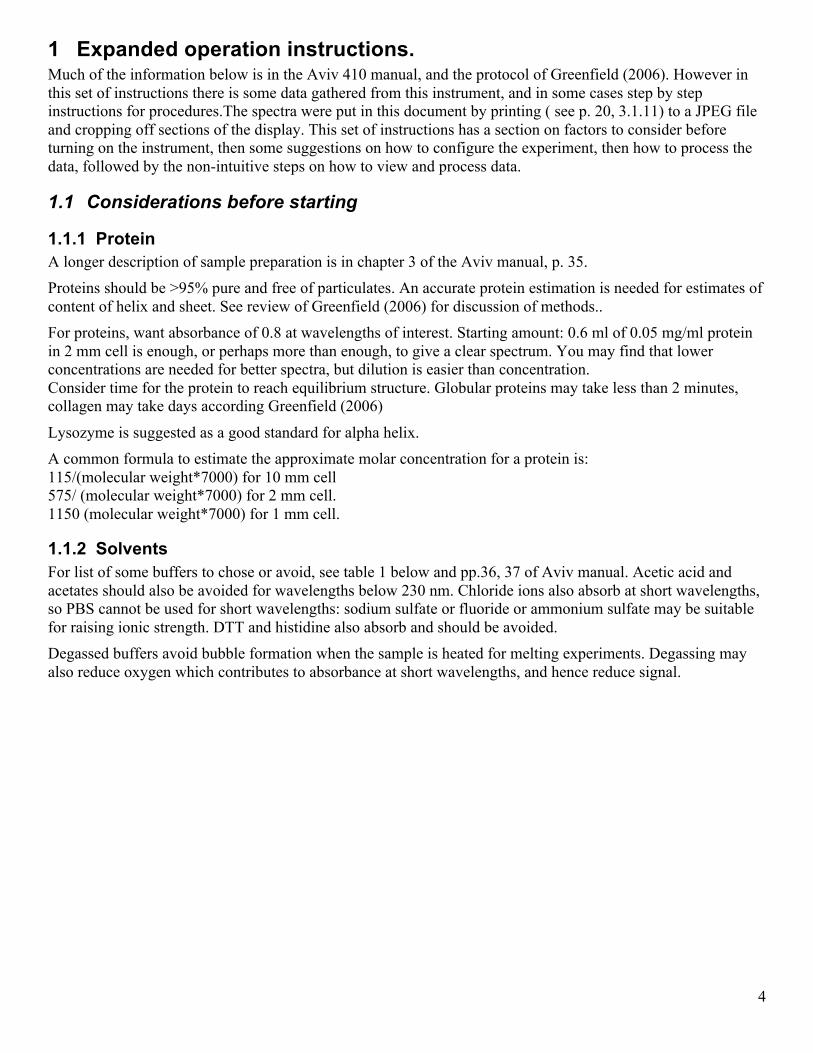
Table 1. Cutoff Wavelengths For Common Solvents and Buffers. Also see pp. 36,37 of Aviv manual Solvent System Cut off (nm) for one mm

path length Water <185 Trifluoroethanol <185 Hexafluoroisopropanol <185 Acetonitrile 185 Methanol 195 Ethanol 196 2-Propanol 196 Cyclohexane <185 Dioxane 232 (NH4)2SO4 0.15 M 191 NaCl 0.15 M 196 NaClO4 0.15 M <185 NaNO3 0.15 M 245 Phosphate 100 mM <185 Tris 100 mM 195 Pipes 100 mM 215 Mes 100 mM 205 GdnHCl 4 M 210 Urea 4 M 210 Water shows significant absorbance at short wavelengths, as shown in absorbance spectra below, which limits the usable wavelength range. Figure 1. Absorbance of water at short wavelengths.

blue trace: water in 2 mm cell green trace: water in 5 mm cell purple trace: water in 10 mm cell. The spectra were calculated from the dynode voltage plots (see p. 18).

6

1.1.3 Cells

1.1.3.1 Path length Short cells (which require higher protein concentrations) minimize absorbance from water and buffers-see p. 5, (Fig 2) 9

For very short path lengths, e.g. 0.1 mm, there are demountable/dismountable cells in two pieces, a tray type piece and a front window. Surface tension and the spring of the holder keep the two pieces together. However Greenfield (2006) warns that the path length of these cells changes with sample viscosity, and they may leak when the temperature changes.

The path length of demountable cells is not necessarily what is stated, with one report showing significant errors in length. Liquid between the two parts of the cell may increase length by 1 µm. To calibrate, see Andrew J. Miles , FrankWiena, Jonathan G. Lees and B.A. Wallace Spectroscopy 19 (2005) 43–51 seen at: http://people.cryst.bbk.ac.uk/~ubcg25a/spectroscopyII.pdf and J.P. Hennessey, Jr. and W.C. Johnson, Jr., Anal. Biochemistry 125 (1982), 177–188. This procedure was unsuccessful for a 2 mm cell using a Beckman 640 spectrophotometer.

1.1.3.2 Cell types From Jack Aviv: “The only cuvettes we recommend for CD is type 111QS. For those who are not interested in temperature studies, type 110QS might suit their needs. We do not recommend them. All cells are made by Hellma, Germany.” Rectangular cells supplied by Hellma either directly or through AVIV, at the same price. Aviv will check that the cells meet their specifications. The 110 series are made by fusing two windows on to a frame. These are adequate for many uses, but the way they are made may leave strains in the cell which reduce optical performance; temperature may affect the cell spectrum-. A Hellma representative said that the Aviv is so sensitive that it can be affected by strains in the 110 series. The 111 series can be used in fluorometers because they are made by joining 4 identical windows giving less strain in the material than the 110 series. The 111 series cost considerably more but are recommended for CD. Another source is New Era (http://www.newera-spectro.com/) which seem cheaper. One user seems happy with them.

1.1.3.3 Sample volumes Table 2

Path length (mm) Minimum volume (µL)

Maximum volume (µL)

10 1800 3300

5 900 ?

2 350 780

1 200 400

It is not clear if the above numbers apply to the Aviv 410. The volume required for the 5 mm cell has been determined here to be between 800 and 1000 µL.

1.1.3.4 Cuvette contamination It is fairly common for protein to remain stuck to a cell. This protein may even make an experiment appear to be a failure.

7

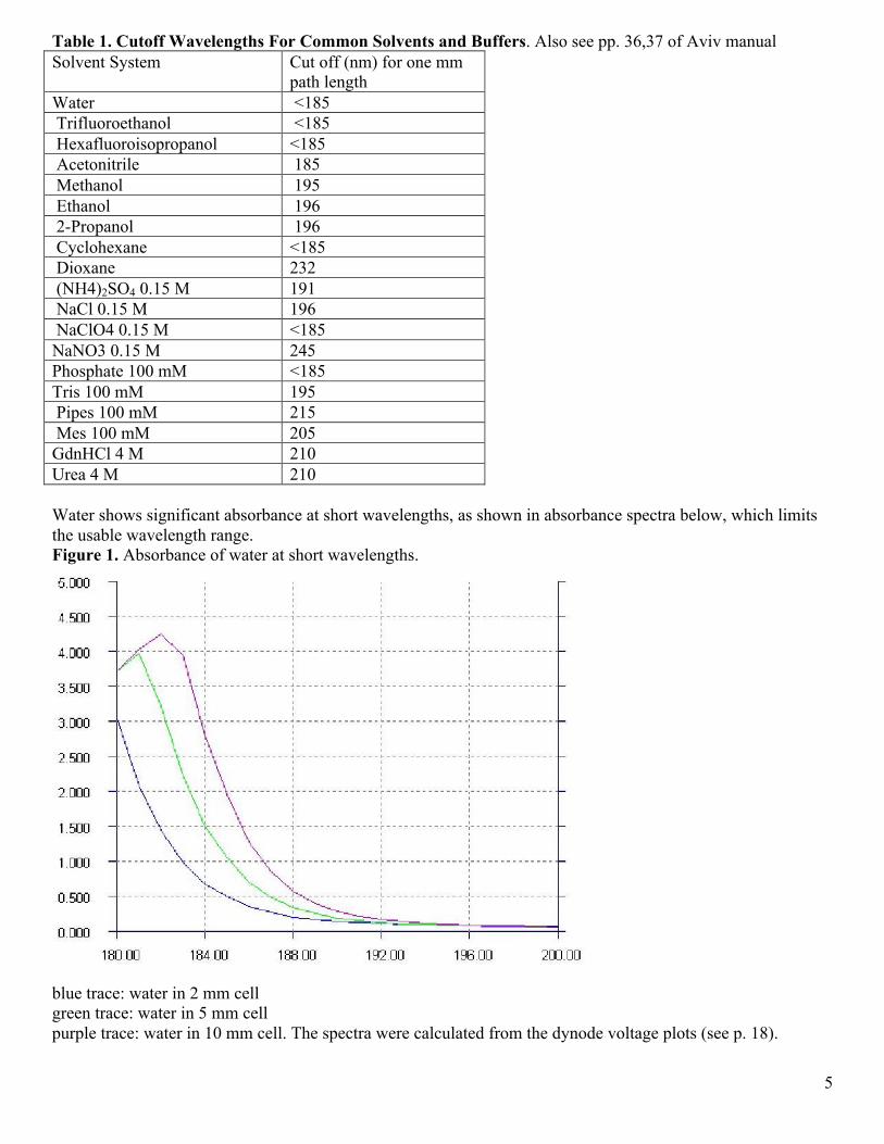
Other contaminants increase the cell absorbance reduce the usable wavelength range. The first test is to take a spectrum in a conventional spectrophotometer. An example of a dirty cell is below. The absorbance (left plot) is higher than seen when the cell was cleaned; the right plot shows a CD spectrum from contamination, possibly from protein left in the cell.

An example of a dirty cell is below. The absorbance (left plot) is higher than seen when the cell was cleaned; the right plot shows a CD spectrum from contamination, possibly from protein left in the cell.

Figure 2. Absorbance and CD spectra of a contaminated cell

Light blue plot is dynode voltage for 2 mm cell, Green is dynode voltage for spectrum of air Dark blue is absorbance, and is similar to what is seen in a regular spectrophotometer.

Dark blue trace; air Green trace, CD signal for previously used cell.

1.1.3.5 Procedures for cleaning cuvettes Protein melting experiments may lead to protein stuck on the cell, and at high concentrations, it may be visible. Some users soak cells in 1% Hellmanex overnight. Shorter washes may work, longer washes may be necessary. Verbally, Jack Aviv suggested Liquinox, SDS, No Chromix. At the back of the Aviv manual are methods for cleaning cells. Another set of methods is in the protocol paper of Greenfield (2006). A direct quote follows: “This procedure can be completed in 10 min or can be done overnight. Cuvettes for CD measurements must be clean and dry. Quartz cells can be cleaned by soaking in: mild detergent solutions available from several cell manufacturers, such as Hellma; a mixture of 30% concentrated HCl and 70% ethanol; or concentrated nitric acid. Protein residues can be dissolved using 6Mguanidine HCl. After soaking, cells should be rinsed with water and ethanol and either dried by suction using an aspirator or blown dry with nitrogen or compressed air that has passed through a filter to remove impurities. If residual proteins are not removed by the previous cleaning agents, filling the cells with Chromerge (a mixture of potassium chromate in concentrated sulfuric acid) (Fisher Scientific cat. no. C577-12; https:// www1.fishersci.com) and immediately rinsing out with water and drying usually is effective. This method is the best method for cleaning cells with 0.01- or 0.02-cm path lengths.” A cell which had a lot of protein stuck in it was not cleaned by a 24 hour soak in 1% Hellmanex. 6M guanidine-HCl overnight did not remove protein, but may have changed the aggregates. 8M urea for several hours also had limited effect. 100 mg/ml ammonium persulfate in 2 M phosphoric acid overnight may have disrupted clumps seen in the cell. 10% SDS for about 2 hours and pushing liquid out of cell (hold upside down, push air into cell with gel loading tip) seemed to remove remaining material. One cell which had high absorbance and an apparent hydrophobic film improved after leaving it in mild detergent for a week.

8

Data for use of Hellmanex from Hellma for cleaning cells: Concentration   Temperature     Time  %  by  vol.   °C       minutes  0.5  -­‐  2       25-­‐30         20-­‐180  0.5  -­‐  2       30-­‐35         30-­‐40  0.5  -­‐  2       50-­‐60  (quartz  only)     10-­‐15  0.5  -­‐  2       70-­‐  80  (quartz  only)   2-­‐5  

An  increase  in  temperature  speeds  up  the  cleaning  process.  However,  at  high  temperatures  it  is  necessary  to  avoid  thermal  shock.  The  cells  should  be  pre-­‐warmed  before  being  submerged  into  hot  cleaning  solutions A suggested aid for cleaning cuvettes is a cuvette cleaner. One is from Fisher catalog 14-385-946A List Price - $138.73 (December 2007)

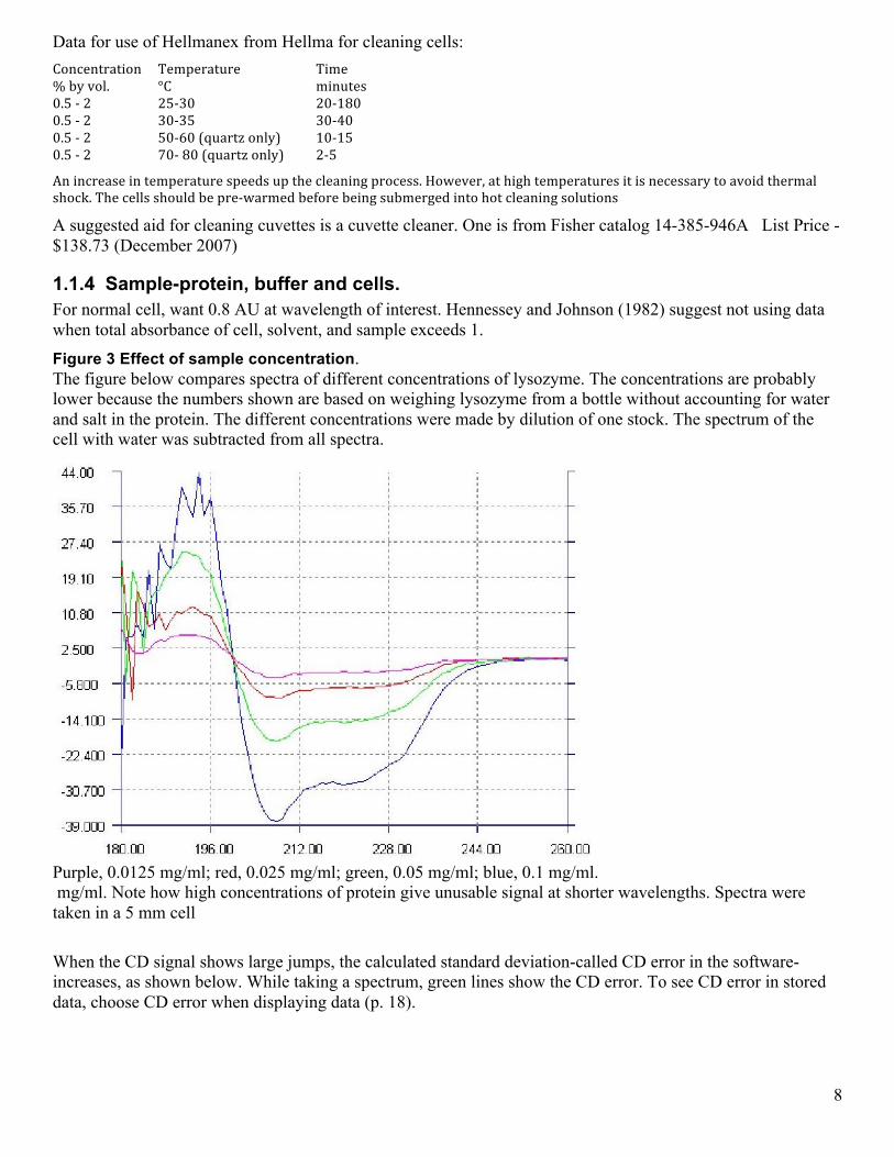
1.1.4 Sample-protein, buffer and cells. For normal cell, want 0.8 AU at wavelength of interest. Hennessey and Johnson (1982) suggest not using data when total absorbance of cell, solvent, and sample exceeds 1. Figure 3 Effect of sample concentration. The figure below compares spectra of different concentrations of lysozyme. The concentrations are probably lower because the numbers shown are based on weighing lysozyme from a bottle without accounting for water and salt in the protein. The different concentrations were made by dilution of one stock. The spectrum of the cell with water was subtracted from all spectra.

Purple, 0.0125 mg/ml; red, 0.025 mg/ml; green, 0.05 mg/ml; blue, 0.1 mg/ml. mg/ml. Note how high concentrations of protein give unusable signal at shorter wavelengths. Spectra were taken in a 5 mm cell

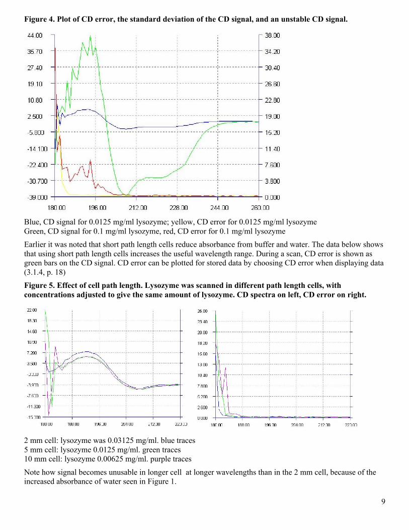
When the CD signal shows large jumps, the calculated standard deviation-called CD error in the software-increases, as shown below. While taking a spectrum, green lines show the CD error. To see CD error in stored data, choose CD error when displaying data (p. 18).

9

Figure 4. Plot of CD error, the standard deviation of the CD signal, and an unstable CD signal.

Blue, CD signal for 0.0125 mg/ml lysozyme; yellow, CD error for 0.0125 mg/ml lysozyme Green, CD signal for 0.1 mg/ml lysozyme, red, CD error for 0.1 mg/ml lysozyme Earlier it was noted that short path length cells reduce absorbance from buffer and water. The data below shows that using short path length cells increases the useful wavelength range. During a scan, CD error is shown as green bars on the CD signal. CD error can be plotted for stored data by choosing CD error when displaying data (3.1.4, p. 18) Figure 5. Effect of cell path length. Lysozyme was scanned in different path length cells, with concentrations adjusted to give the same amount of lysozyme. CD spectra on left, CD error on right.

2 mm cell: lysozyme was 0.03125 mg/ml. blue traces 5 mm cell: lysozyme 0.0125 mg/ml. green traces 10 mm cell: lysozyme 0.00625 mg/ml. purple traces

Note how signal becomes unusable in longer cell at longer wavelengths than in the 2 mm cell, because of the increased absorbance of water seen in Figure 1.

10

1.1.5 Plan for wavelength scan Scan the cell alone, and cell with buffer in a spectrophotometer to see how much absorbance there is. If this is satisfactory, and you have sample to use, scan the sample also. This data may tell you what wavelength range you can use. If the cell has excessively high absorbance, see 1.1.3.5 p. 7 for ways to clean it. If the cell with buffer has acceptable spectra, plan to run a wavelength scan on the cell with buffer before running a scan of a protein. If you are using a two piece demountable cell, you may want to estimate the actual path length which may be significantly different from the marked length. (1.1.3.1 p. 6). If spectrophotometer data is satisfactory, in the CD, scan Air (reference) Cell with buffer. Sample.

11

2 Operation Nitrogen supply. The lamp converts oxygen to ozone which damages the optics and hence needs to be purged from the monochromator and other parts. Finding a suitable source of nitrogen has been surprisingly complex even though CD has been around for decades. The most common solution is a tank of liquid nitrogen. With infrequent use, most of the nitrogen boils off and escapes to atmosphere. We had a problem with unexpectedly high levels of oxygen in the nitrogen which reached our instrument, resulting in major optical damage. Because the measured levels were higher than expected, and a meter to measure levels costs over $7000, and CD use is infrequent, we chose to use cylinders of high purity nitrogen. Nitrogen On nitrogen cylinder (left of CD), open valve on cylinder. Note cylinder pressure on right gauge; pressure drops about 200 p.s.i. per hour that nitrogen flows..

1. Open valves on the black nitrogen scrubber cartridge (handles and cartridge will point in a line). There is an indicator after the cartridge to show if the scrubbing cartridge is exhausted. The scrubbing cartridge is to remove any oxygen which comes from the tank but is expensive and should not be used to avoid having high purity nitrogen supply. If the indicator is yellow, replace scrubber cartridge. Red is satisfactory. Flow meter next to regulator should be at 20 .

Pressure should be 20 p.s.i. Flow on gauge should be 20. If there is no flow, see if the valves on the scrubber cartridge are open. A block inside the instrument controls distribution to different parts of the instrument. Turn on 30 minutes before lamp. If there is insufficient nitrogen, contact John Shannon, room 232, ph. 3-9399, email jds1c@virginia.edu..

2. Turn on water bath; it should be set at 20°C. Complete instructions at back of Aviv manual. The water bath is to remove heat from the Peltier temperature control unit and is left set at 20°C. If it is not, push left button on front briefly-a longer push will take you to the settings for temperature high and low limits. Change temperature with middle two keys. Key on far right is for the timer and temperature ramping. If there is no cooling, see if the cooling switch on the back is on. If there are beeps from high temperature, hold down left button until there is an option to change the high limit. Use up key to increase it.

3. After 30 minutes, of purging with nitrogen, turn on switch for XE LAMP PWR..

4. Power control green light on the power supply (lower shelf, right) will light, and within a minute, the lamp ready light. If other lights come on, there may be no nitrogen flow, or other parts of the instrument are turned on or temperature is too high. When both lights are on, briefly press the red start button. The meter should show current flowing and a light should show the lamp is on. If not, try again.

5. Turn on the CPU switch on the instrument, then turn on computer and monitor. Ensure temperature control power supply next to computer (vertical box) is on-green light next to switch should be illuminated. If it is not on, there will be an error message about the thermo-electric controller.

6. Select the user account. Selection from the menu is a little slow because of the number of accounts. Pressing Ctrl-Alt-Del may bring up a log on screen a little faster.

7. Instrument control program is cdsxm, desktop shortcut CDS or Aviv 410. The program cdsmxd is for data analysis only, and may be installed on other computers (p. 20). If you try to use it to run the instrument, the data will look strange. The icon for this program has been changed on the desktop and start menu to CDS Data Viewer.

12

8. If you create a configuration file which will have settings for data path, wavelength range etc.: it is quicker to load than rewriting settings. go to File-read configuration file. To create a configuration file, after making your settings, go to File-save configuration. You must enter a name and .cfg extension.

9. Software operation is mainly the same as for model 215, but there is an auto save option for data (under Configure experiment-Experiment configuration-save data option.). If you change wavelength on the experiment configuration page, the program will be unresponsive until the monochromator has changed to the wavelength you set.

2.1 Settings for operation If you have made a configuration file with data path and scan settings, load the file (File-read configuration file). When entering numbers in fields, press Enter after writing the number or else it may not be saved.

2.1.1 Data storage Data will be stored in the last folder used, probably by the previous user. To set default folder for data storage, go to Displays-data browser: In the Default Dataset Path box at the bottom of the window, either type in folder name AND Press Enter or open Windows Explorer/My Computer, (icon may be on Quick Launch toolbar ), navigate to the folder you want (e.g C:\Data\lab_name), highlight the path in the address bar near top of screen and copy the path (Ctrl-C), switch back to the Data Browser window, highlight the current address, paste the patch in the Default Dataset Path box (Ctrl-V) AND press Enter. If you do not press Enter, the change will not be saved. Close the window. Set up experiment with from the Configure experiment menu.

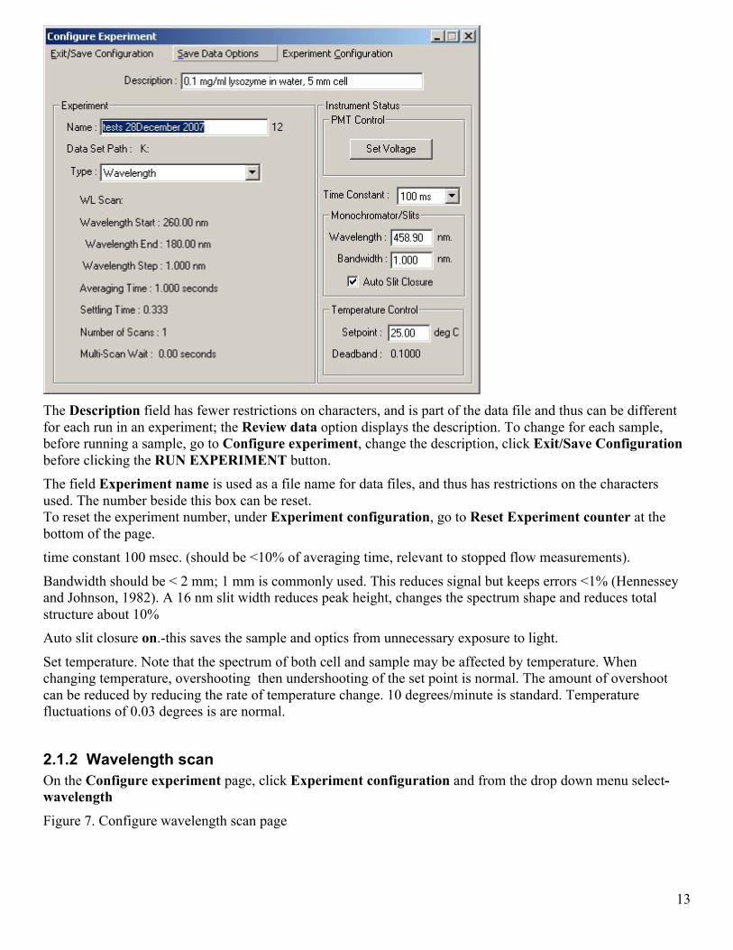
Figure 6. Configure experiment page

13

The Description field has fewer restrictions on characters, and is part of the data file and thus can be different for each run in an experiment; the Review data option displays the description. To change for each sample, before running a sample, go to Configure experiment, change the description, click Exit/Save Configuration before clicking the RUN EXPERIMENT button. The field Experiment name is used as a file name for data files, and thus has restrictions on the characters used. The number beside this box can be reset. To reset the experiment number, under Experiment configuration, go to Reset Experiment counter at the bottom of the page. time constant 100 msec. (should be <10% of averaging time, relevant to stopped flow measurements).

Bandwidth should be < 2 mm; 1 mm is commonly used. This reduces signal but keeps errors <1% (Hennessey and Johnson, 1982). A 16 nm slit width reduces peak height, changes the spectrum shape and reduces total structure about 10% Auto slit closure on.-this saves the sample and optics from unnecessary exposure to light.

Set temperature. Note that the spectrum of both cell and sample may be affected by temperature. When changing temperature, overshooting then undershooting of the set point is normal. The amount of overshoot can be reduced by reducing the rate of temperature change. 10 degrees/minute is standard. Temperature fluctuations of 0.03 degrees is are normal.

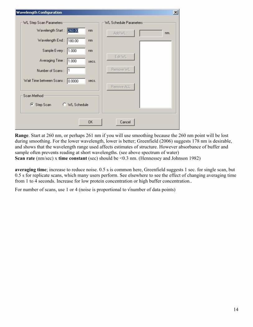
2.1.2 Wavelength scan On the Configure experiment page, click Experiment configuration and from the drop down menu select-wavelength

Figure 7. Configure wavelength scan page

14

Range. Start at 260 nm, or perhaps 261 nm if you will use smoothing because the 260 nm point will be lost during smoothing. For the lower wavelength, lower is better; Greenfield (2006) suggests 178 nm is desirable, and shows that the wavelength range used affects estimates of structure. However absorbance of buffer and sample often prevents reading at short wavelengths. (see above spectrum of water) Scan rate (nm/sec) x time constant (sec) should be <0.3 nm. (Hennessey and Johnson 1982) averaging time; increase to reduce noise. 0.5 s is common here, Greenfield suggests 1 sec. for single scan, but 0.5 s for replicate scans, which many users perform. See elsewhere to see the effect of changing averaging time from 1 to 4 seconds. Increase for low protein concentration or high buffer concentration..

For number of scans, use 1 or 4 (noise is proportional to √number of data points)

15

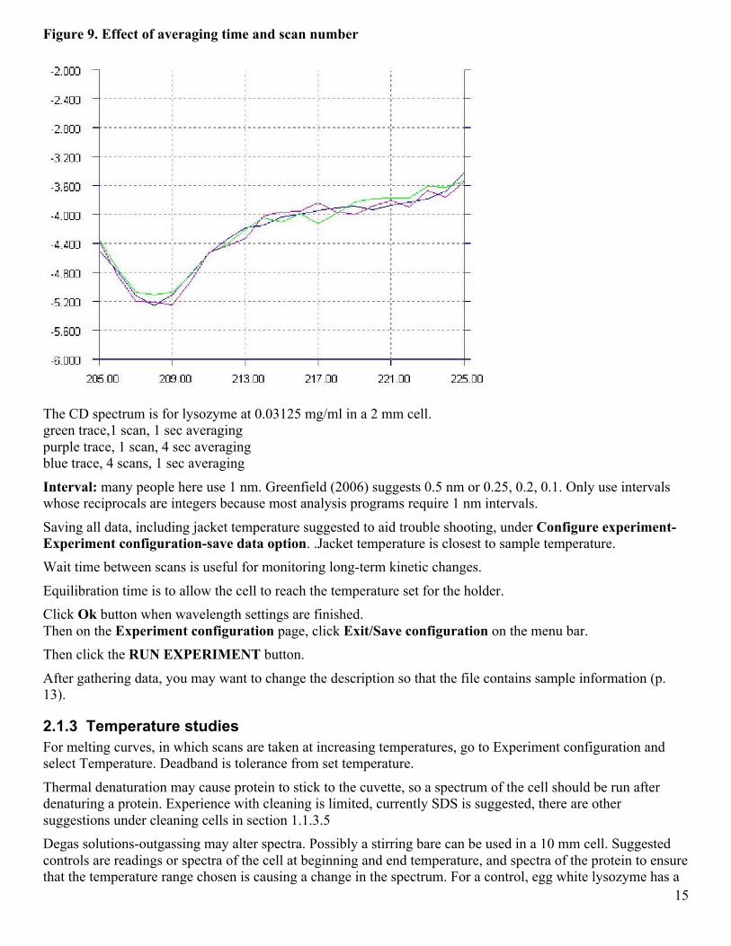
Figure 9. Effect of averaging time and scan number

The CD spectrum is for lysozyme at 0.03125 mg/ml in a 2 mm cell. green trace,1 scan, 1 sec averaging purple trace, 1 scan, 4 sec averaging blue trace, 4 scans, 1 sec averaging

Interval: many people here use 1 nm. Greenfield (2006) suggests 0.5 nm or 0.25, 0.2, 0.1. Only use intervals whose reciprocals are integers because most analysis programs require 1 nm intervals.

Saving all data, including jacket temperature suggested to aid trouble shooting, under Configure experiment-Experiment configuration-save data option. .Jacket temperature is closest to sample temperature. Wait time between scans is useful for monitoring long-term kinetic changes.

Equilibration time is to allow the cell to reach the temperature set for the holder. Click Ok button when wavelength settings are finished. Then on the Experiment configuration page, click Exit/Save configuration on the menu bar. Then click the RUN EXPERIMENT button.

After gathering data, you may want to change the description so that the file contains sample information (p. 13).

2.1.3 Temperature studies For melting curves, in which scans are taken at increasing temperatures, go to Experiment configuration and select Temperature. Deadband is tolerance from set temperature.

Thermal denaturation may cause protein to stick to the cuvette, so a spectrum of the cell should be run after denaturing a protein. Experience with cleaning is limited, currently SDS is suggested, there are other suggestions under cleaning cells in section 1.1.3.5 Degas solutions-outgassing may alter spectra. Possibly a stirring bare can be used in a 10 mm cell. Suggested controls are readings or spectra of the cell at beginning and end temperature, and spectra of the protein to ensure that the temperature range chosen is causing a change in the spectrum. For a control, egg white lysozyme has a

16

transition temperature of 74°C in 10 mM phosphate pH 7; Worthington lysozyme recommended over Sigma by Aviv but Sigma product showed a change.

For fluorescence need HV set point to get FL signal of 1 (volt).

2.1.4 Saving data Data can be automatically saved while running. Configure experiment-Experiment configuration-save data option. Data can be automatically saved to hard disk but may ask about overwriting. Choose the place to save your data from data browser.

17

2.2 running sample Before each scan, you can identify the data file with sample information by going to Configure experiment, change the description, click Exit/Save Configuration before clicking the RUN EXPERIMENT button

Handling cells with gloves is recommended. Transfer pipettes work with large cells, gel loading tips for short cells.

Select a cell and holder for 1, 2 or 5 mm cells. Note which side of the cell faces forward so that for further readings, you have the cell in the same orientation.

Push cell completely down; a pen is a suitable object to push the cell all the way to the bottom of the compartment. Scan air as a reference. Scan empty dry cell to see how much absorbance and CD signal the cell has. Scan buffer. Problems: Sometimes the lamp shuts off, giving noisy signal. Power supply will show no current drawn by lamp. If the signal is a steady 260 mdeg, you may have used the data review program. If signal is very noisy, absorbance may be too high. Signal to noise ratio increases with photomultiplier /dynode voltage, and 500V has been cited (Greenfield) as a point at which there is a major increase.

18

3 Evaluating data 3.1.1 Data handling For data viewing only, turn on CPU switch on instrument. Use program CDSMXD whose shortcut now says analysis. The data can be viewed in the AVIV software, or opened in Excel. Instructions to install CDSMXD on other computers are later (p. 20).

3.1.2 Loading data from disk Start Data viewer (cdsmxd) The message about stopped flow calibration apparently can be ignored. Go to Displays-data browser. It may be easier to find data if you set a default data path to where your data is stored at the bottom of the window; the path name needs to be typed in or loaded from a configuration file (see p. 12) Click button read data set<disk and select file using conventional navigation techniques Hold down the Ctrl key while clicking up to 8 files. After choosing the data, a progress bar shows briefly. You can load more files. However it is not obvious that you have loaded data. Next go to Displays-data review to select the type of data to show. e.g. wavelength.

3.1.3 Viewing sample information To see sample information, after loading data above, under Displays-data browser, in the right panel, click on the experiment type, e.g. Wavelength experiments clicking on the + sign if present. Keep expanding the list by clicking on + signs until you can select the data you want, e.g. CD dynode, or CD signal, and the Review data set button on the left turns black. Click that button. Alternatively, open data set to get to data, open the data file with another program e.g. Notepad, or OpenOffice.

3.1.4 Viewing data Before viewing data, go to Displays-Data Review and select data type e.g. Wavelength. Then go to Axis definitions and click left multi-data set to show more than one CD signal. You can select left axis definition, but the multi-data set allows you to easily add more data. Choose the signals to display Choose right multi-data set to show another set of data e.g. dynode voltage on the same plot but with a different scale. To set range, move the mouse pointer into the plot area and right click just inside the axis; at some point, a window will open. To remove a plot, Axis definitions-clear left axis definition. Setting color for the lines is not as convenient as some other programs; it is under Axis definitions-Trace color configuration.

3.1.5 Calculating absorbance. Run a scan of air as reference, then the cell. To calculate absorbance, go to math operations-wavelength experiments. For data set A, choose CD dynode of the scan of the empty cell. Then choose operation- convert dynode to absorbance. Then choose data set B, dynode for the scan of air. Enter a name for the absorbance spectrum. Click the Calculate button. The manual calculation is roughly log (V2/V1) x 7.4 An example of the absorbance of a cell is Fig. 2.

19

3.1.6 Data quality At short wavelengths, data is unreliable because signals are weak because of absorbance of sample, buffer, water, cell. If the signal jumps wildly, it is useless. If the dynode voltage has reached a plateau, the data is unreliable. When the dynode voltage is above 640, the accuracy of the signal is reduced. If dynode voltage is above 740, the signal is inaccurate. A plateau suggests that the instrument is detecting only stray light. Useful signals are 1 decade less than stray light. On this instrument, if dynode voltage is 800, the signal is probably useless. Green bars on CD trace are standard deviation of reading. To see the standard deviation of the CD signal in data which is stored, when viewing data, choose CD error for the sample of interest. A problem with estimates of structure are that the total amounts of different structures can total more than 100%. See Hennessey and Johnson (1982) for sources of errors.

3.1.7 Averaging spectra To average spectra, load and view data (3.1.4 p. 18, 18. Then open Axis definitions-data review average. -Select the spectra to average. Go back to Axis definitions-data review average In the panel Resulting data set, in the box Experiment, enter a new file name, -using the same name as used for collection will overwrite raw data. However, you need to go back to Displays-data browser to save the file to disk. Under Save data set > disk. The averaged signal may automatically display, using the right axis scale, even though the average trace is not listed as being displayed using either left or right axes. You can set the right axis scale to be the same as the left, or save the average signal, close the program, and reload the average trace from the saved file. or To remove the average trace from the display, go to Data review average and click the Clear average trace button. The colors used for different traces can be seen under Axis definitions-clear left axis definitions.

3.1.8 Subtracting a blank Open data as above. Then go to Math operations and select the type of data e.g. Wavelength experiments. Click on the button Select data set A. In the window that appears, keep clicking on + signs until you can select the data you want, (no more + signs, buttons to left darken and become active) which may be an average signal. Click the Select Data set button. Next go to the Operation or constant panel, and in the Operation box, select Subtract data sets from the drop down list. Then click the button Select data set B. You must choose the operation before selecting the data set, otherwise you have to start again. Select the second spectrum. In the Results panel, enter a file name, click calculate and return. Go back to Data browser and save the data to disk.

3.1.9 Smoothing Aviv in their manual suggest that smoothing does not help the data. It also removes data points from the final set because the first and last points in the data set are used in smoothing, and cannot be smoothed themselves. However Greenfield (2006) suggests smoothing.

3.1.10 Using Excel To import into Excel, start Excel and open file. Choose Files of type- all files (*.*). In the text import wizard, choose the Fixed width option. In the data display, scroll down until you can see the spectral data, and make and adjust the columns. For a standard wavelength spectrum, you will have to add two column breaks. To plot, select the wavelength and signal data, and under chart (Insert-chart or toolbar icon), select XY scatter.

20

3.1.11 Printing data Choices..

1. Print with printer. When using the File-print screen command, drag the dialog box (white background, print screen) off the plot area, otherwise there will be a blank area. Note that the printer has to be set in Windows, and cannot be chosen in the Aviv programs.

2. Print to an image file from Data reviewer File-print screen. Go to Windows Start button, then Settings-Printers and Faxes. Right click PDFCreator and set as default. in Aviv data review, use the File-print screen command; you will be asked for a file to save the screen picture in. In the save as type box, select an image type (pdf, JPG, tif) for saving. Reset default printer to DeskJet. At one time, using PDF Creator led to continual requests to provide Microsoft Office installation CD. To get around this problem, (a) open Microsoft Office (it may be necessary to use Windows Task Manager to stop the installation program). This problem seems to occur if Microsoft office has not been used in the account you are using. (b) insert the Office installation disk. There should be a copy in the back of the instrument manual. If this does not work, it may be because the account you are in does not have administrative rights. If the solution above does not work, probably a computer administrator will have to change your account so you can perform the installation.

3. To put the plot directly into a file, press Alt-PrintScreen keys. Open Windows Paint, then Edit-paste. Save the file, and it can be edited with other programs. This method does not have the legends or white background available from the File-print screen command. Printing to an image file with PDFCreator has advantages but is more complex.

4. Plot data in Excel.

3.1.12 Installing CDSMXD for data analysis on other computers. Installation on other computers is not fully understood, so the instructions below may not work as written. Create directory C:\AVIV. Copy CDSMXD.exe file to C:\AVIV Copy other configuration files AB0109.TE; CDSDEF3.CFG, CDSDEF.TSN, CDSDEF.HW, TECFG.EXE. These may not all be necessary. The program wants to have read/write access to C:\AVIV because default configuration files are created and saved to this directory. Start cdsmxd, saying yes to the option to load stopped low syringe driver . From within the CDSMX program, go to 'Control Panels' -> 'Instrument Configuration' -> 'Device Configuration'. The 'PMT Gain' value on the left side of the dialog should be set to 7.067. If the Ok button is grayed out, in one case it seemed that there was no attempt to load the stopped flow syringe control; however this explanation did not hold in another case. On another installation, the files, AB0109.TE; CDSDEF3.CFG, CDSDEF.TSN, CDSDEF.HW were read only; removing read only restriction seemed to cause the PMT gain to become 7.067 instead of 0, although the value could still could not be saved.

3.1.13 Deconvoluting data to estimate structure Inaccurate wavelength settings can cause errors. Hennessey and Johnson show that a 2 nm error in wavelength changed the total structure amount by 10% for lactate dehydrogenase. Anti-parallel sheet was changed in the

21

opposite direction from other structure types. Estimates of beta turn are little affected by wavelength errors, helix is sensitive. Increased bandwidth can also cause errors . Hennessey and Johnson recommend bandwidth < 2 nm. Fast scan rates and big time constants will distort spectra. With a time constant of 10 seconds, speeds up to 2 nm/min are nearly identical, but faster scan rates shift peaks and reduce intensity; the examples shows a 15% decrease in total structure at a scan rate of 16 nm/min.(Hennessey and Johnson 1982). Time constant (sec) x scan rate (nm/sec) should be less than 0.33. .Incorrect intensity readings have a linear effect on total structure and individual structure types. Green bars on CD trace are standard deviation of reading. On stored data, this information can be seen when viewing data by choosing CD error Inaccurate path lengths will give inaccurate data. For a calibration procedure, see p. 6 Sample concentration errors will also give inaccurate data. Note that weighing a protein from a bottle may overestimate the amount of protein because of salts and water in the protein. Greenfield (2006) has a comprehensive discussion of choices for estimating protein concentration. Hennessey and Johnson 1982 suggest A190, amino acid analysis, ninhydrin assay. Errors in signal can occur from instrument calibration errors, and failure to correct for baseline, and drift. To minimize baseline errors, scan cell under same conditions as sample, with the same orientation of the cell (Aviv manual pp. 37-39). Hennessey and Johnson 1982 show changes in structure estimates from incorrectly aligning baseline. Drift can also cause a problem, so multiple scans with a low time constant are better than one long scan. Running baselines before and after the sample may show if drift is occurring. Hennessey and Johnson suggest that if your data uses different wavelength range from standards, the structure estimate will differ. A number of programs exist. Greenfield (2006) compares estimates by several programs, and the effect of the wavelength range used. A link to software for deconvolution http://www2.umdnj.edu/cdrwjweb/index.htm#software For material with a large amount of beta helix, -synthetic polypeptides, amyloids, collagen, coiled-coiled proteins, the preferred programs are LINCOMB, K2D, CONTIN. The program commonly used is CDNN. To use it, data from the CD instrument needs some preparation. If you have the data, you need to average scans, subtract blank, smooth, and convert a signal in millidegrees to molar ellipticity. Most of these calculations can be done in Excel, but using the Aviv Data viewer program may be easier. Note that the CDNN program needs data up to 260 nm.

3.1.13.1 Preparing data for deconvolution. Procedure based on instructions from Sam Yun.

1. Start Aviv “Data Viewer” Program (cdsmxd) Ignore the load stopped flow syringe driver control program message, and the warning message that follows afterward).

2. go to the Displays menu, and select Data Browser. 3. Set default directory by typing in the path to your data, and press enter 4. Click Read data set <-Disk. 5. Select your data file(s).

a. Sometimes the program does not recognize a file that has too long path file name. For instance, C:\data\document and settings\Samuel\research\sando\lab\cddata\010306\Ghrelin\TFEsolution\50percent\TFE50percent010306baseline.dat. The above file will most likely NOT be able to read by the program. In this

22

case, simply copy the file into a simpler path. For instance, C:/TFE50percent010306baseline.dat The above path will be read by the program.

6. While the data is loaded, you will be able to see blue bar going across your screen to show the data reading process.

7. In the same data browser window, expand the Wavelength Experiments into sub data by clicking the + boxes until you see a line CD Signal for each scan run..

8. If you ran 3 scans, there should be ‘Scan #1’. Scan #2, Scan #3. Etc. 9. To average data, see earlier instructions on p. 19. 10. Repeat above steps to average the buffer scans. 11. Once you have the averaged signal scan and the averaged buffer scan, you need to subtract the buffer

scan from signal scan. 12. You can do this by going to Math Operations on the top menu. 13. Click Wavelength experiment. 14. Click on Select Data Set A. 15. Select your averaged or raw signal scan. You may need to expand the list of data sets by clicking the +

signs. After finding the data, click the Select Data Set button. 16. In the Operation or Constant box, select an operation from the drop down list. In this case, subtract

data sets. 17. Click on Select Data Set B 18. Select your buffer scan. 19. In the Data set name. e.g.. “baseline subtracted” 20. click on Calculate. 21. Then may smooth the data (opinions differ about the wisdom of doing so). 22. smooth the data set by following these steps. 23. select data set A, which would be “baseline subtracted” data set. 24. select Smoothing on Operation 25. Write the data set name. Ex. “ Data baseline subtracted smoothed” 26. click on calculate 27. Then you need to convert the data to Molar ellipticity. 28. Uner Math Operations, click select data set A -e.g. Data baseline subtracted smoothed.Again you

may need to expand the list of data by clicking on + signs. 29. In the Operation box, choose convert to molar ellipticity. 30. write data set name ex. “baseline subtracted smoothed ME” 31. click calculate (if nothing happens, it may be because you pressed keys in the wrong order), 32. on the window that pops up. Write the following data.

a. # of amino acids. b. Molar concentration: c. Cell length: (cm)

33. For a protein with much alpha helix, expect numbers of 10,000 deg cm2 dmol-1 at 190 nm, -10,000 at 208 nm (order of magnitude numbers).

34. Now you need to export the saved data into .txt file. 35. select Displays-Data Browser 36. Expand the Wavelength Experiments list by clicking + signs, until you see the averaged, baseline

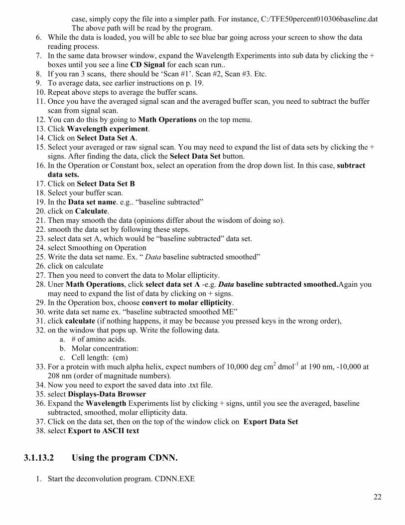
subtracted, smoothed, molar ellipticity data. 37. Click on the data set, then on the top of the window click on Export Data Set 38. select Export to ASCII text

3.1.13.2 Using the program CDNN.

1. Start the deconvolution program. CDNN.EXE

23

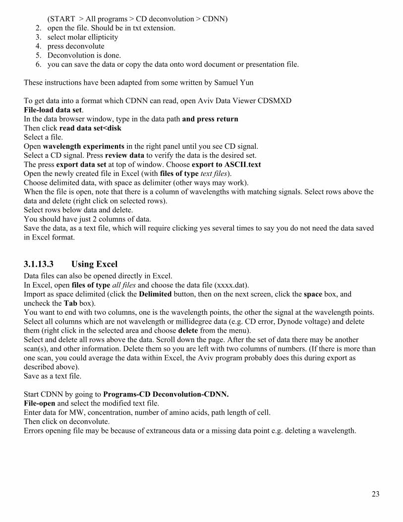
(START > All programs > CD deconvolution > CDNN) 2. open the file. Should be in txt extension. 3. select molar ellipticity 4. press deconvolute 5. Deconvolution is done. 6. you can save the data or copy the data onto word document or presentation file.

These instructions have been adapted from some written by Samuel Yun To get data into a format which CDNN can read, open Aviv Data Viewer CDSMXD File-load data set. In the data browser window, type in the data path and press return Then click read data set<disk Select a file. Open wavelength experiments in the right panel until you see CD signal. Select a CD signal. Press review data to verify the data is the desired set. The press export data set at top of window. Choose export to ASCII.text Open the newly created file in Excel (with files of type text files). Choose delimited data, with space as delimiter (other ways may work). When the file is open, note that there is a column of wavelengths with matching signals. Select rows above the data and delete (right click on selected rows). Select rows below data and delete. You should have just 2 columns of data. Save the data, as a text file, which will require clicking yes several times to say you do not need the data saved in Excel format.

3.1.13.3 Using Excel Data files can also be opened directly in Excel. In Excel, open files of type all files and choose the data file (xxxx.dat). Import as space delimited (click the Delimited button, then on the next screen, click the space box, and uncheck the Tab box). You want to end with two columns, one is the wavelength points, the other the signal at the wavelength points. Select all columns which are not wavelength or millidegree data (e.g. CD error, Dynode voltage) and delete them (right click in the selected area and choose delete from the menu). Select and delete all rows above the data. Scroll down the page. After the set of data there may be another scan(s), and other information. Delete them so you are left with two columns of numbers. (If there is more than one scan, you could average the data within Excel, the Aviv program probably does this during export as described above). Save as a text file. Start CDNN by going to Programs-CD Deconvolution-CDNN. File-open and select the modified text file. Enter data for MW, concentration, number of amino acids, path length of cell. Then click on deconvolute. Errors opening file may be because of extraneous data or a missing data point e.g. deleting a wavelength.

24

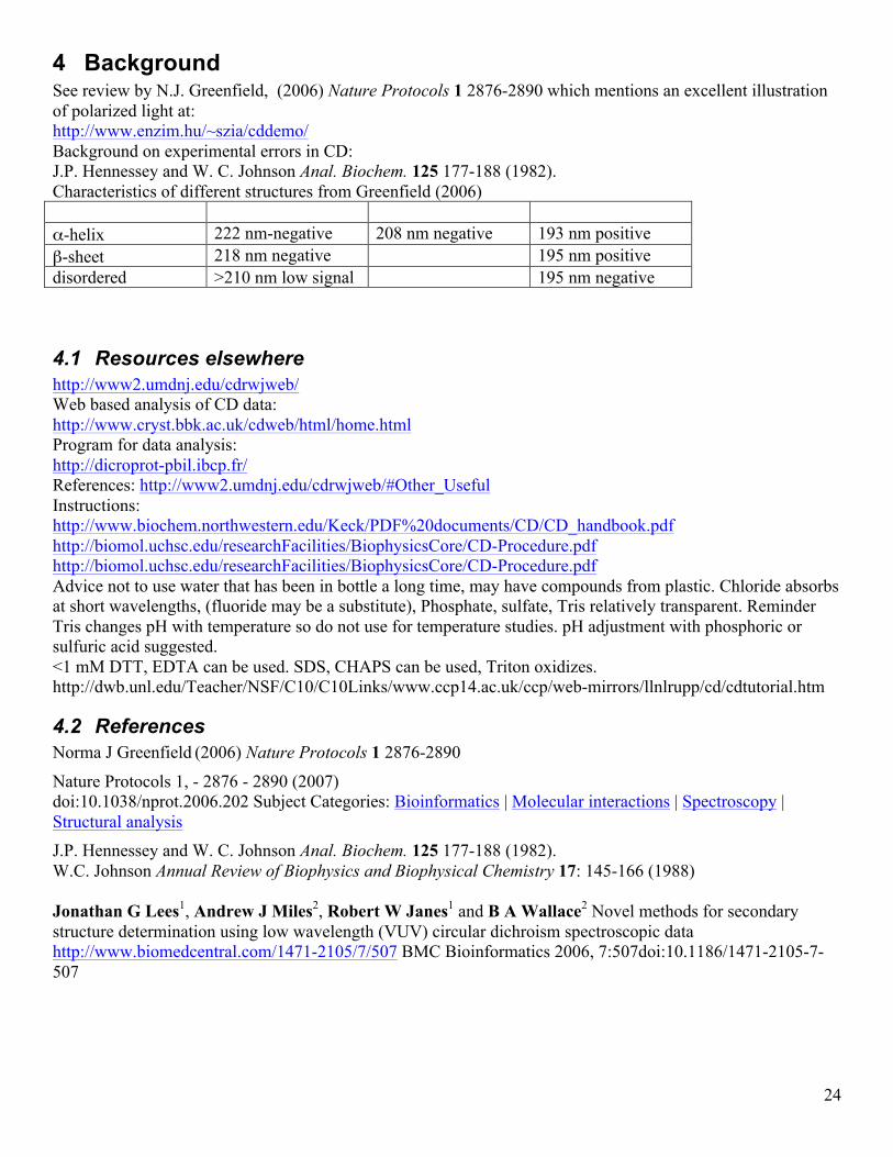
4 Background See review by N.J. Greenfield, (2006) Nature Protocols 1 2876-2890 which mentions an excellent illustration of polarized light at: http://www.enzim.hu/~szia/cddemo/ Background on experimental errors in CD: J.P. Hennessey and W. C. Johnson Anal. Biochem. 125 177-188 (1982). Characteristics of different structures from Greenfield (2006) α-helix 222 nm-negative 208 nm negative 193 nm positive β-sheet 218 nm negative 195 nm positive disordered >210 nm low signal 195 nm negative

4.1 Resources elsewhere http://www2.umdnj.edu/cdrwjweb/ Web based analysis of CD data: http://www.cryst.bbk.ac.uk/cdweb/html/home.html Program for data analysis: http://dicroprot-pbil.ibcp.fr/ References: http://www2.umdnj.edu/cdrwjweb/#Other_Useful Instructions: http://www.biochem.northwestern.edu/Keck/PDF%20documents/CD/CD_handbook.pdf http://biomol.uchsc.edu/researchFacilities/BiophysicsCore/CD-Procedure.pdf http://biomol.uchsc.edu/researchFacilities/BiophysicsCore/CD-Procedure.pdf Advice not to use water that has been in bottle a long time, may have compounds from plastic. Chloride absorbs at short wavelengths, (fluoride may be a substitute), Phosphate, sulfate, Tris relatively transparent. Reminder Tris changes pH with temperature so do not use for temperature studies. pH adjustment with phosphoric or sulfuric acid suggested. <1 mM DTT, EDTA can be used. SDS, CHAPS can be used, Triton oxidizes. http://dwb.unl.edu/Teacher/NSF/C10/C10Links/www.ccp14.ac.uk/ccp/web-mirrors/llnlrupp/cd/cdtutorial.htm

4.2 References Norma J Greenfield (2006) Nature Protocols 1 2876-2890

Nature Protocols 1, - 2876 - 2890 (2007) doi:10.1038/nprot.2006.202 Subject Categories: Bioinformatics | Molecular interactions | Spectroscopy | Structural analysis J.P. Hennessey and W. C. Johnson Anal. Biochem. 125 177-188 (1982). W.C. Johnson Annual Review of Biophysics and Biophysical Chemistry 17: 145-166 (1988)

Jonathan G Lees1, Andrew J Miles2, Robert W Janes1 and B A Wallace2 Novel methods for secondary structure determination using low wavelength (VUV) circular dichroism spectroscopic data http://www.biomedcentral.com/1471-2105/7/507 BMC Bioinformatics 2006, 7:507doi:10.1186/1471-2105-7-507