Ba7202 financial management (unit1) notes

Financial Management Semester II

S.N.Selvaraj, Assistant Professor, E-mail: [email protected] Page 1

UNIT – I: FOUNDATIONS OF FINANCE

Financial Management – An Overview – Time Value of Money – Introduction to the

Concept of Risk and Return of a Single Asset and of a Portfolio – Valuation of Bonds

and Shares – Option Valuation

FINANCIAL MANAGEMENT

Financial Management is that managerial activity which is concerned with the

planning and controlling of the firm‟s financial resources. It was a branch of

economics till 1890 and as a separate discipline, it is of recent origin.

Finance may be defined as the provision of money at the time when it is required.

Finance refers to the management of flows of money through an organization. It

concerns with the application of skills in the manipulation, use and control of money.

Definition and Meaning of Financial Management

According to F.W.Paish,“Finance may be defined as the position of money at the time

it is wanted”.

According to the John J Hampton, “The term finance can be defined as the

management of flows of money through an organization, whether it will be a

corporation, school, bank or government agency”.

According to Weston & Brigham, “Financial management is an area of financial

decision making harmonizing individual motives and enterprise goals.

Evolution of Financial Management

Traditional Phase: In the traditional phase the focus of financial management was on

certain events which required funds e.g. major expansion, merger, reorganization etc.

It is also characterized by a heavy emphasis on legal and procedural aspects as at that

point of time the functioning of companies was regulated by a plethora of legislation.

Transitional Phase: During the transitional phase the nature of financial management

was the same but more emphasis was laid on problems faced by finance managers in

the areas of fund analysis, planning and control.

Modern Phase: The modern phase is characterized by the application of economic

theories and the application of quantitative methods of analysis.

AN OVERVIEW OF FINANCIAL MANAGEMENT

Financial management has undergone significant changes, over the years in its scope

and coverage. Its approach measures the scope of the finance in various fields, which

include the maximization of wealth of an organization.



Objectives of Finance

The management of finance is to achieve financial objectives. The following are the

main objectives of finance

To create wealth for business

To generate cash

To provide adequate return of investment (bearing in mind the risk of

business and the resources invested)

To ensure that sufficient fund is provided at right time to meet the needs

of the business

Scope of Finance

What is finance? What are a firm‟s financial activities? How are they related to the

firm‟s other activities? Firms create manufacturing capacities for production of goods;

some provide services to customers. They sell their goods or services to earn profit.

They raise funds to acquire manufacturing and other facilities. Thus, the three most

important activities of a business firm are:

Production

Marketing

Finance

A firm secures whatever capital it needs and employs it (finance activity) in activities,

which generate returns on invested capital (production and marketing activities).

Functions of Financial Management

The functions of raising funds, investing them in assets and distributing returns earned

from assets to shareholders are respectively know as financing decision, investment

decision and dividend decision.

Long-term financial decisions:

Long-term asset-mix or investment decision

Capital-mix or financing decision

Profit allocation or dividend decision

Short-term financial decisions:

Short-term asset-mix or liquidity decision

Functions of Financial Management

Investment Decision Finance Decision

Dividend Decision Liquidity Decision



Investment Decisions: A firm‟s investment decisions involve capital

expenditures. They are therefore referred as capital budgeting decisions.

There is a broad agreement that the correct cut-off rate or the required rate of

return on investments is the opportunity cost of capital. The opportunity cost

of capital is the expected rate of return that an investor could earn by investing

his or her money in financial assets of equivalent risk.

Financing Decisions: A financing decision is the second important function to

be performed by the financial manager. He or she must decide when, where

from and how to acquire funds to meet the firm‟s investment needs. The mix

of debt and equity is known as the firm‟s capital structure. The financial

manager must strive to obtain the best financing mix or the optimum capital

structure for his or her firm.

Dividend Decisions: A dividend decision is the third major financial decision.

The financial manager must decide whether the firm should distribute all

profits or retain them or distribute a portion and retain the balance. The

proportion of profits distributed as divided is called the dividend-payout ratio

and the retained portion of profits is known as the retention ratio.

Liquidity Decision: Investment in current assets affects the firm‟s profitability

and liquidity. Management of current assets that affects a firm liquidity is yet

another important finance function. A proper trade-off must be achieved

between profitability and liquidity. The profitability-liquidity trade-off

requires that the financial manger should develop sound techniques of

managing current assets.

Role of Financial Management in the Organization

Finance and Management Functions:There exists an inseparable relationship between

finance on the one hand and production, marketing and other functions on the other.

Almost all business activities directly or indirectly, involve the acquisition and use of

funds. For example, recruitment and promotion of employees in production is clearly

a responsibility of the production department; but it requires payment of wages and

salaries and other benefits and thus, involves finance.

Real and Financial Assets:A firm requires real assets to carry on its business. Tangible

real assets are physical assets that include plant, machinery, office, factory, furniture

and building. Intangible real assets include technical know-how, technological

collaborations, patents and copyrights.

Financial assets, also called securities, are financial papers or instruments such as

shares and bonds or debentures. Firms issue securities to investors in the primary

capital markets to raise necessary funds. The securities issued by the firms are traded

– bought and sold – by investors in the secondary capital markets, referred to as stock

exchanges.



Equity and Borrowed Funds:There are two types of funds that a firm can raise: equity

funds (simply called equity) and borrowed funds (called debt). A firm sells shares to

acquire equity funds. Shares represent ownership rights of their holders. Buyers of

shares are called shareholders (or stockholders) and they are legal owners of the firm

whose shares they hold. Shareholders invest their money in the shares of a company in

the expectation of a return on their invested capital. The return consists of dividend

and capital gain. Shareholders make capital gains (or losses) by selling their shares.

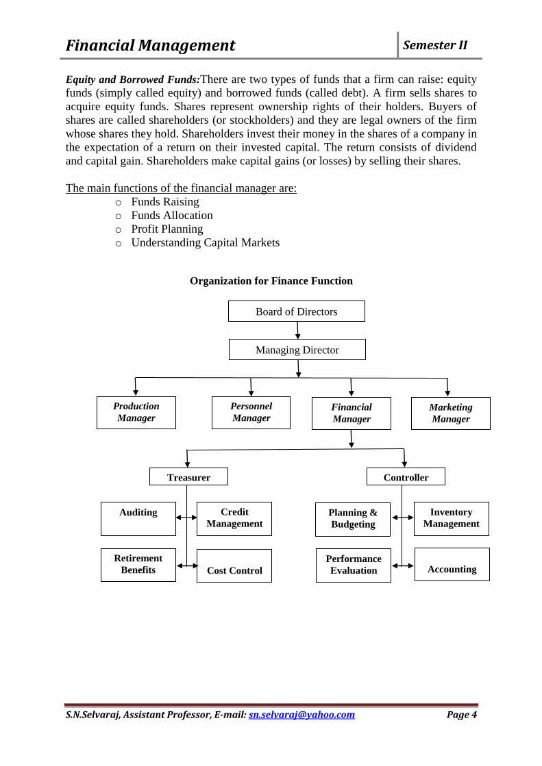
The main functions of the financial manager are:

o Funds Raising

o Funds Allocation

o Profit Planning

o Understanding Capital Markets

Organization for Finance Function

Board of Directors

Managing Director

Production

Manager

Personnel

Manager Financial

Manager

Marketing

Manager

Treasurer Controller

Credit

Management Planning &

Budgeting

Auditing Inventory

Management

Cost Control

Retirement

Benefits Performance

Evaluation

Accounting



TIME VALUE OF MONEY

The concept of TVM refers to the fact that the money received today is different in its

worth from the money receivable at some other time in future. In other words, the

same principle can be stated as that the money receivable in future is less valuable

than the money received today. For example, if an individual is given an option to

receive Rs.1000 today or to receive the same amount after one year, he will definitely

choose to receive the amount today.

The obvious reason for this reference for receiving money today is that the rupee

received today has a higher value than the rupee receivable in future. This preference

for current money as against future money is known as the time preference for money

or simply time value of money. Cash flows can be either positive or negative; positive

cash flows are called cash inflows and negative cash flows are called cash outflows.

Time Preference for Money

If an individual behaves rationally, he or she would not value the opportunity to

receive a specific amount of money now, equally with the opportunity to have the

same amount at some future date. Most individuals value the opportunity to receive

money now higher than waiting for one or more periods to receive the same amount.

Time Preference of Money or Time Value of Money (TVM) is an individual‟s

preference for possession of a given amount of money now, rather than the same

amount at some future time.

Three reasons may be attributed to the individual‟s time preference for money.

Risk

Preference for consumption

Investment opportunities

FUTURE VALUE

Let us assume that an investor requires 10 percent interest rate to make him different

to cash flows one year apart. The question is how should he arrive at comparative

values of cash flows that are separated by two, three or any number of years?

Once the investor has determined his interest rate, say, 10 percent, he would

like to receive at least Rs.1.10 after one year or 110 percent of the original

investment of Re 1 today. A two year period is two successive one-year

periods. When the investor invested Re1 for one year, he must have received

Rs.1.10 back at the end of that year in exchange for the original Re1. If the

total amount so receive (Rs.1.10) were reinvested, the investor would expect

1.10 percent of that amount, or rs.1.21 = Re1 * 1.10 * 1.10 at the end of the

second year.

Notice that for any time after the first year, he will insist on receiving interest on the

first year‟s interest as well as interest on the original amount (principal).



Compound Interestis the interest that is received on the original amount

(principal) as well as on any interest earned but not withdrawn during earlier

periods. Compounding is the process of finding the future values of cash flows

by applying the concept of compound interest.

Simple Interestis the interest that is calculated only on the original amount

(principal) and thus, no compounding of interest takes place.

Future Value of a Single Cash Flow

Suppose your father gave you Rs.100 on your eighteenth birthday. You deposited this

amount in a bank at 10 percent rate of interest for one year. How much future sum

would you receive after one year? You would receive Rs.110:

Fn = P (1 +i)n

Future sum = Principal + Interest

= 100 + (0.10 *100)

= 100 * (1.10) = Rs.110

What would be the future sum if you deposited Rs.100 for two years? You would

now receive interest on interest earned after one year:

Future sum = 100 * 1.10 * 1.10 = Rs.121

You could similarly calculate future sum for any number of years. We can express

this procedure of calculating compound or future value in formal terms.

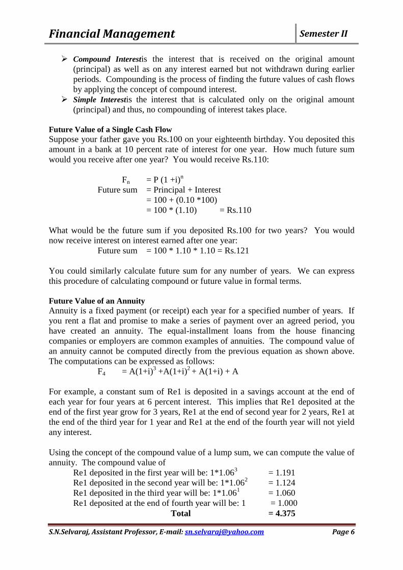
Future Value of an Annuity

Annuity is a fixed payment (or receipt) each year for a specified number of years. If

you rent a flat and promise to make a series of payment over an agreed period, you

have created an annuity. The equal-installment loans from the house financing

companies or employers are common examples of annuities. The compound value of

an annuity cannot be computed directly from the previous equation as shown above.

The computations can be expressed as follows:

F4 = A(1+i)3 +A(1+i)

2 + A(1+i) + A

For example, a constant sum of Re1 is deposited in a savings account at the end of

each year for four years at 6 percent interest. This implies that Re1 deposited at the

end of the first year grow for 3 years, Re1 at the end of second year for 2 years, Re1 at

the end of the third year for 1 year and Re1 at the end of the fourth year will not yield

any interest.

Using the concept of the compound value of a lump sum, we can compute the value of

annuity. The compound value of

Re1 deposited in the first year will be: 1*1.063 = 1.191

Re1 deposited in the second year will be: 1*1.062 = 1.124

Re1 deposited in the third year will be: 1*1.061 = 1.060

Re1 deposited at the end of fourth year will be: 1 = 1.000

Total = 4.375



PRESENT VALUE

However, it is a common practice to translate future cash flows into their present

values. Present value of a future cash flow (inflow or outflow) is the amount of

current cash that is of equivalent value to the decision maker. Discountingis the

process of determining present values of a series of future cash flows. The compound

interest rate used for discounting cash flows is also called the discount rate.

Present Value of a Single Cash Flow

As we have seen earlier that an investor with an interest rate i, of say, 10 percent per

year, would remain indifferent between Re1 now and Re1*1.101 = Rs1.10 one year

from now and Re1*1.102 = Rs1.21 after two years and Re1*1.10

3 = Rs1.33 after 3

years.

We can say that, given 10 percent interest rate, the present value of Rs.1.10 after one

year is Re1; of Rs.1.21 after two years is Re.1 and so on.

Assuming a 10 percent interest rate, we know that an amount sacrificed in the

beginning of the year will grow to 110 percent or 1.10 after a year. Thus the amount

to be sacrificed today would be: 1/1.10 = Rs.0.909. In other words, at a 10 percent

rate, Re.1 to be received after a year is 110 percent of Re.0.909 sacrificed now. Stated

differently, Re.0.909 deposited now at 10 percent rate of interest will grow to Re.1

after one year. If Re.1 is received after two years, then the amount needed to be

sacrificed today would be 1/1.102 = Rs.0.826.

How can we express the present value calculations formally? Let I represent the

interest rate per period, n the number of periods, F the future value (or cash flow) and

P the present value (cash flow). We know the future value after one year, F1 (viz.,

present value (principal) plus interest), will be: F1 = P(1+i)

The present value, P will be = P = F1/ (1+i)1

The future value after two years is = F2 = P(1+i)2

The present value, P will be = P = F2 / (1+i)2

The present values can be worked out for any combination number of years and

interest rate. The following general formula can be employed to calculate the present

value of a lump sum to be received after some future periods:

P = Fn/ (1+i)n = Fn [(1+i)

−n]

P = Fn/ (1+i)n

The term in parentheses is the discount factor or present value factor (PVF) and it is

always less than 1.0 for positive I, indicating that a future amount has a smaller

present value. We can rewrite Equation as follows:

Present value = Future value*Present value factor of Re1

PV = Fn* PVFni



PVFni is he present value factor for n periods at i rate of interest. When we want to

calculate the present value factor, we can use a scientific calculator. Alternatively we

can use of a table of pre-calculated present value factors. Simply, to find out the

present value of future amount, find out the present value factor (PVF) for given n and

I from the calculated table and multiply by the future amount.

For example, an investor wants to find out the present value of Rs.50000 to be

received after 15 years. The interest rate is 9 percent. First, we will find out the

present value factor from the calculated table as 0.275 and multiply by Rs.50000; we

obtain Rs.13750 as the present value.

PV = 50000*PVF15 = 50000*0.275 = Rs.13750

Present Value of Annuity

An investor may have an opportunity of receiving an annuity – a constant periodic

amount – for a certain specified number of years. We will have to find out the present

value of the annual amount every year and will have to aggregate all the present

values to get the total present value of the annuity.

For example, an investor, who has a required interest rate as 10 percent per year, may

have an opportunity to receive an annuity of Rs.1 for four years.

The present value of Rs.1 received after one year is, P = 1/(1.10) = Rs.0.909,

After two years, P = 1/(1.10)2 = Rs.0.826, after 3 years, P = 1/(1.10)

3 = Rs.0.751 and

After four years, P = 1/(1.10)4 = Rs.0.683.

Thus the total present value of an annuity of Rs.1 for four years is Rs.3.169 as shown

below.

P = [1/(1.10) + 1/(1.10)2 +1/(1.10)

3 +1/(1.10)

4]

= [0.909 + 0.826 + 0.751 + 0.683 = Rs.3.169

The computation of the present value of an annuity can be written in the following

general form:

P = A[1/i − 1/i (1+i)n]

The term within parentheses of above equation is the present value factor of an

annuityof Rs.1, which we would call PVFA and it is a sum of single-payment present

value factors.

For example, assume that a person receives an annuity of Rs.5000 for four years. If

the rate of interest is 10 percent, the present value of Rs.5000 annuity is calculated as

follows:

P = A[1/i − 1/i (1+i)n]

P = 5000 [1/0.10 − 1/0.10 (1.10)4]

= 5000 * (10 − 6.830) = 5000 * 3.170 = Rs.15,850



It can be realized that the present value calculations of an annuity for a long period

would be extremely cumbersome without a scientific calculator. We can use the table

of pre-calculated present values of an annuity of given present value of annuity of

Rs.1 for numerous combinations of time periods and rates of interest.

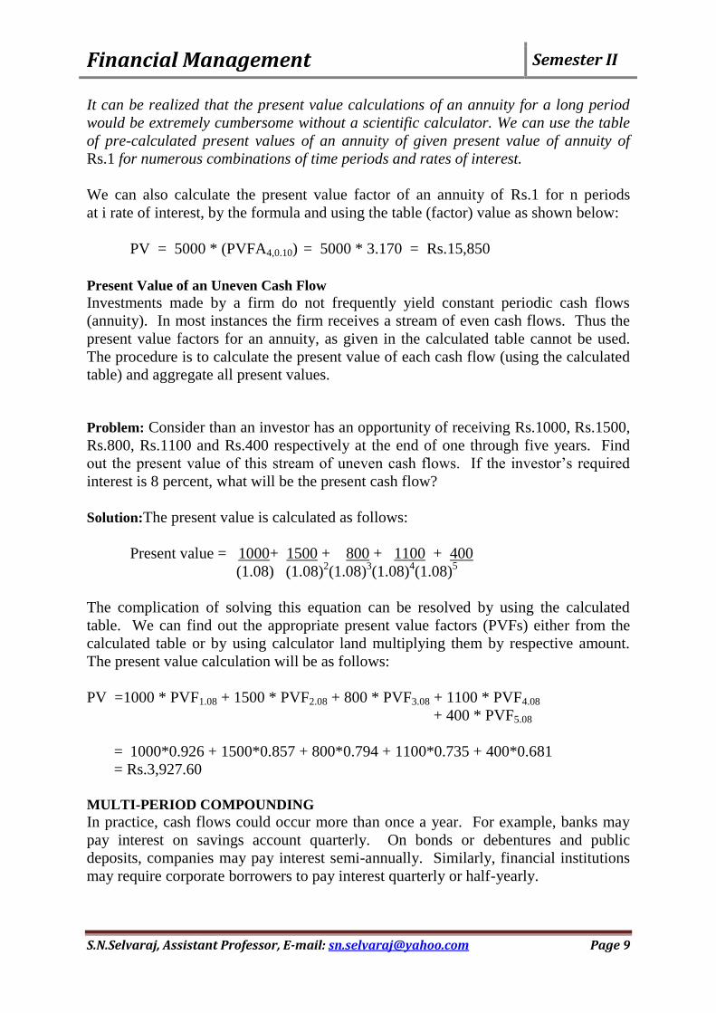
We can also calculate the present value factor of an annuity of Rs.1 for n periods

at i rate of interest, by the formula and using the table (factor) value as shown below:

PV = 5000 * (PVFA4,0.10) = 5000 * 3.170 = Rs.15,850

Present Value of an Uneven Cash Flow

Investments made by a firm do not frequently yield constant periodic cash flows

(annuity). In most instances the firm receives a stream of even cash flows. Thus the

present value factors for an annuity, as given in the calculated table cannot be used.

The procedure is to calculate the present value of each cash flow (using the calculated

table) and aggregate all present values.

Problem: Consider than an investor has an opportunity of receiving Rs.1000, Rs.1500,

Rs.800, Rs.1100 and Rs.400 respectively at the end of one through five years. Find

out the present value of this stream of uneven cash flows. If the investor‟s required

interest is 8 percent, what will be the present cash flow?

Solution:The present value is calculated as follows:

Present value = 1000+ 1500 + 800 + 1100 + 400

(1.08) (1.08)2(1.08)

3(1.08)

4(1.08)

5

The complication of solving this equation can be resolved by using the calculated

table. We can find out the appropriate present value factors (PVFs) either from the

calculated table or by using calculator land multiplying them by respective amount.

The present value calculation will be as follows:

PV =1000 * PVF1.08 + 1500 * PVF2.08 + 800 * PVF3.08 + 1100 * PVF4.08

+ 400 * PVF5.08

= 1000*0.926 + 1500*0.857 + 800*0.794 + 1100*0.735 + 400*0.681

= Rs.3,927.60

MULTI-PERIOD COMPOUNDING

In practice, cash flows could occur more than once a year. For example, banks may

pay interest on savings account quarterly. On bonds or debentures and public

deposits, companies may pay interest semi-annually. Similarly, financial institutions

may require corporate borrowers to pay interest quarterly or half-yearly.



The interest rate is usually specified on an annual basis, in a long agreement or

security (such as bonds) and is known as the nominal rate of interest. If compounding

is done more than once a year, the actual annualized rate of interest would be higher

than the nominal interest rate and it is called the effective interest rate.

Problem:

You can get an annual rate of interest of 13 percent on a public deposit with a

company. What is the effective rate of interest if the compounding is done (a) half-

yearly, (b) quarterly, (c) monthly and (d) weekly? Calculate EIR.

Solution:

The general formula for calculating EIR can be written in the following general form:

EIR = [1+i/m]nm

– 1 where „i‟ is the annual nominal rate of interest,

„n‟ the number of years and

„m‟ the number of compounding per year.

In annual compounding, m = 1, in monthly compounding, m = 12 and in

weekly compounding m = 52.

Effective Interest Rate (EIR)

(a) EIR = [1+0.13/2]1*2

– 1 = (1.065)2 – 1 = 1.1342 – 1 = 0.1342

or 13.42%

(b) EIR = [1+0.13/4]1*4

– 1 = (1.0325)4 – 1 = 1.1365 – 1 = 0.1365

or 13.65%

(c) EIR = [1+0.13/12]1*12

– 1= (1.01083)12

– 1 = 1.1380 – 1 = 0.1380

or 13.80%

(d) EIR = [1+0.13/52]1*52

– 1= (1.0025)52

– 1 = 1.1386 – 1 = 0.1386

or 13.86%

______________________________________ Problem: (Multi-period Compounding)

Find out the compound value of Rs.1000, interest rate being 12 percent per annum if

compounded annually, semi-annually, quarterly and monthly for 2 years.

Annual compounding

Fn = 1000[1+0.12/1]2*1

= 1000(1.12)2 = 1000*1.254 = Rs.1254

Half-yearly compounding

Fn = 1000[1+0.12/2]2*2

= 1000(1.06)4 = 1000*1.262 = Rs.1262

Quarterly compounding

Fn = 1000[1+0.12/4]2*4

= 1000(1.03)8 = 1000*1.267 = Rs.1267

Monthly compounding

Fn = 1000[1+0.12/12]2*12

= 1000(1.01)24

= 1000*1.270 = Rs.1270



INTRODUCTION TO THE CONCEPT OF RISK AND RETURN OF A SINGLE

ASSET AND OF A PORTFOLIO

Concept of Risk

The risk simply means the possibility of loss or damage, the degree or probability of

such loss. Risk is composed of the demand that bring in variations in return of income.

The main forces contributing to risk are price and interest. All investments are risky,

whether in stock or capital market or banking and financial sector, real estate, bullion

gold, etc.

Definition of Risk

According to Fischer and Jordon, “Risk is the variability of return around the

expected average is thus a quantitative description of risk”.

According to Cornelius Keating, “Risk is the unwanted subset of a set of uncertain

outcomes”.

Causes of Risk

1) Wrong Decision: Wrong decision of what to invest in.

2) Wrong Timing: Wrong timing of investments.

3) Nature of Instruments: Nature of instruments invested such as shares or bonds,

chit funds, benefit funds are highly risky than bank deposits or postal

certificates, etc.

4) Creditworthiness of Issuer: Securities of government and semi-government

bodies are more creditworthy than those issued by the corporate sector.

5) Maturity Period (or) Length of Investment: Longer the period, the more risky is

the investment normally.

6) Amount of Investment: Higher the amount invested in any security the larger is

the risk.

7) Method of Investment: Method of investment, namely, secured by collateral or

not.

8) Terms of Lending: Terms of lending such as periodicity of servicing,

redemption periods, etc.

9) Nature of Industry: Nature of industry or business in which the company is

operating.

10) National and International Factors: The factors prevailing in the nation and

abroad in terms of acts of goods, etc.



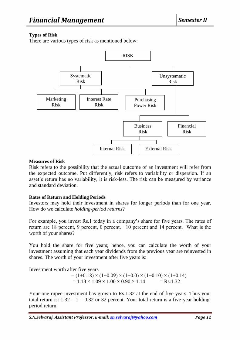
Types of Risk

There are various types of risk as mentioned below:

Measures of Risk

Risk refers to the possibility that the actual outcome of an investment will refer from

the expected outcome. Put differently, risk refers to variability or dispersion. If an

asset‟s return has no variability, it is risk-less. The risk can be measured by variance

and standard deviation.

Rates of Return and Holding Periods

Investors may hold their investment in shares for longer periods than for one year.

How do we calculate holding-period returns?

For example, you invest Rs.1 today in a company‟s share for five years. The rates of

return are 18 percent, 9 percent, 0 percent, −10 percent and 14 percent. What is the

worth of your shares?

You hold the share for five years; hence, you can calculate the worth of your

investment assuming that each year dividends from the previous year are reinvested in

shares. The worth of your investment after five years is:

Investment worth after five years

= (1+0.18) × (1+0.09) × (1+0.0) × (1−0.10) × (1+0.14)

= 1.18 × 1.09 × 1.00 × 0.90 × 1.14 = Rs.1.32

Your one rupee investment has grown to Rs.1.32 at the end of five years. Thus your

total return is: 1.32 – 1 = 0.32 or 32 percent. Your total return is a five-year holding-

period return.

RISK

Systematic

Risk Unsystematic

Risk

Purchasing

Power Risk

Marketing

Risk

Interest Rate

Risk

Business

Risk

Financial

Risk

Internal Risk External Risk



Problem: Variance and Standard Deviation

The shares of Hypothetical Company Limited have the following anticipated returns

with associated probabilities. What is the expected rate of return?

Return (%): −20 −10 10 15 20 25 30

Probability: 0.05 0.10 0.20 0.25 0.20 0.15 0.05

Solution

The expected rate of return is:

E(R) =(−20 ×0.05) + (−10 ×0.10) + (10 ×0.20) + (15 ×0.25) +

(20 ×0.20) + (25 ×0.15) + (30 ×0.05)

= 13%

The risk, measured in terms of variance and standard deviation, is:

σ2 = [(−20– 13)]

20.05 + [(−10– 13)]

20.10 + [(10– 13)]

20.20 + [(15–13)]

20.25

+ [(20–13)]20.20 + [(25–13)]

20.15 + [(30–13)]

20.05

= 156

σ = √156 = 12.49%

Risk Preference

A risk-averse investor will choose from investments with the equal rates of return, the

investment with lowest standard deviation. Similarly, if investments have equal risk

(standard deviations), the investor would prefer the one with higher return. A risk-

neutral investor does not consider risk and he would always prefer investments with

higher returns. A risk-seeking investor likes investments with higher risk irrespective

of the rates of return.

Utility Risk-seeker

Risk-neutral

Risk-averse

Risk Risk Preference

Meaning of Return

The objective of any investor is to maximize expected returns from his investments,

subject to various constrains, primarily risk. Return is the motivating force, inspiring

the investor in the form of rewards for undertaking the investment. The importance of

returns in any investment decision can be traced to the following factors.



It enables investors to compare alternative investments in terms of what they

have to offer the investor.

Measurement of historical or past returns enables the investors to assess how

well they have done.

Measurement of historical returns also helps in estimation of future returns.

Types of Return

There are two types which are as follows:

o Realized Return:This is ex-post (after the fact) return, or return that was or

could have been earned. For example, a deposit of Rs.1000 in a bank on

January 1, at a stated annual interest rate of 10% will be worth Rs.1100 exactly

a year later. The historical or realized return in this case is 10%.

o Expected Return: This is the return from an asset that investors anticipate or

expect to earn over some future period. The expected return is subject to

uncertainty or risk and may or may not occur. The investor compensates for the

uncertainty in returns and the timing of those returns by requiring an expected

return that is sufficiently high to offset the risk or uncertainty.

Components of Return

The return of an investment consists of two components.

Current Return:The first component that often comes to mind when one is

thinking about return is the periodic cash flow (income), such as dividend or

interest generated by the investment. Current return is measured as the periodic

income in relation to the beginning price of the investment.

Capital Return:The second component of return is reflected in the price change

called the capital return. It is simply the price appreciation (or depreciation)

divided by the beginning price of the asset. For assets like equity stocks, the

capital return predominates.

Measure of Return

1) Traditional Method

2) Modern Method

TRADITIONAL METHODS

Computation of yield to measure a financial asset‟s return is the simplest and oldest

technique of measurement. Yield can be found out by the following ways:

Estimated Yield = Expected Cash Income / Current Price of Assets

Actual Yield = Cash Income / Amount Invested

Problem

An investor buys a bond in 2010 maturity in 2012 at Rs.900. It has a maturity value

of 10 years and par value of Rs.1000. It fetches Rs.90 every year. Calculate yield.

Solution

Current Yield = Annual Cash Price / Purchase Price



= 90 / 900 = 10%

Yield to Maturity = Average Annual Return / Average Investment

= 100 / 950 = 0.105 or 10.5%

C = Annual Coupon

M = Maturity of par value of bond

P = Purchase Price

N = Number of years remaining to maturity

Average Annual Return = C +[(M−P)/N]

= 90 + [1000−900)/10]

= 90 + 10 = 100

Average Investment = (M+P)/2

= (1000+900)/2

= 1900/2 = 950

The return of stock or share is measured by finding out dividend yield. Dividend

yields can be estimated on expected yields as well as actual yields.

Estimated Yield = Expected Cash Dividend / Current Share price

Actual Yield = Dividend Received / Price of the share in the beginning

(or)

Earning Yield = Earning / Price of Share

Problem: A stock that is selling for Rs.36 and earns Rs.3 annually has an E/P ratio of

what?

Solution

Earning Yield = Earning / Price of Share

= 3/36 =0.083 or 8.33%

RISK AND RETURN

Financial decisions incur different degree of risk. Your decision to invest the money

in government bonds has less risk as interest rate is known and the risk of default is

very less. On the other hand, you would incur more risk if you decide to invest the

money in shares, as return is not certain. However, you can expect a lower return

from government bond and higher from shares. Risk and expected return move in

tandem; the greater the risk, the greater the expected return. The following figure

shows this risk-return relationship.



An Overview of Financial Management

Trade-off

Risk-free rate is a rate obtainable from a default-risk free government security. An

investor assuming risk from her investment requires risk premium above the risk-free

rate. Risk-free rate is a compensation for time and risk premium for risk. Higher the

risk of action, higher will be the risk premium leading to higher required return on that

action. A proper balance between return and risk should be maintained to maximize

the market value of a firm‟s shares.

VALUATION OF BONDS AND SHARES

A bond is a contract that requires the borrower to pay the interest income to the

lender. It resembles the promissory note issued by the government and corporate. The

par value of the bond indicates the face value of the bond i.e. the value stated on the

bond paper. Generally, the face values of bonds are Rs.1000, Rs.2000, Rs.5000 and

alike. Most of the bonds are make fixed interest payment till the maturity period.

Thus, security can be valued in the following form;

1) Bond

2) Equity Shares

3) Preference Shares

4) Derivative Instrument like Options

FINANCIAL MANAGEMENT

Maximization of Share Value

Financial Decision

Investment

Decisions

Liquidity

Management

Financing

Decisions

Dividend

Decisions

Return Risk



Features of Bond or Debentures

Face Value is called par value. A bond or debenture is generally issued at a par

value of Rs.100 or Rs.1000 and interest is paid on face value.

Interest Rate is fixed and known to bondholders (debenture-holders). Interest

paid on a bond / debenture is tax deductible. The interest rate is also called

coupon rate. Coupons are detachable certificates of interest.

Maturity A bond (debenture) is generally issued for a specified period of time.

It is repaid on maturity.

Redemption Value is the value that a bondholder (debenture-holder) will get on

maturity is called redemption or maturity, value. A bond (debenture) may be

redeemed at par or at a premium (more than par value) or at a discount (less

than par value).

Market Value A bond (debenture) may be traded in a stock exchange. The price

at which it is currently sold or bought is called the market value. Market value

may be different from par value or redemption value.

VALUATION OF BOND Present Value of Bond

The value of a bond – or any asset, real or financial – is equal to the present value of

the value of cash flows expected from it. So determining the intrinsic value of a bond

requires:

(i) An estimated of expected cash flow,

(ii) An estimate of the required return.

The value of the bond is calculated as:

n

P = ∑ [C÷(1+r)t] + [M÷(1+r)

n]

t=1

Where, P = value (in rupees)

n = number of years

C = annual coupon payment (in rupees)

r = periodic required return rate

M = maturity value

t = time period when the payment is received

We can also apply the formula by using present value of an ordinary annuity.

P = C × PVIFAr,n + M × PVIFr,n

For example, consider a 10 year, 12 percent coupon bond with a par value of Rs.1000.

The required yield on this bond is 13 percent. The cash flows for this bond are as

follows:

10 annual coupon payment of Rs.120

Rs.1000 principal repayment 10 years from now

The value of the bond is:

P = C × PVIFA13%,10yrs + M × PVIF13%,10yrs



= 120 × 5.426 + 1000 × 0.295

= 651.1 + 295 = Rs.946.1

Bond Yield

The word yield is frequently used with regard to investing in bonds. Bonds are

generally traded on the basis of their prices. However they are usually not compared

in terms of prices because of significant variations in cash flow patterns and other

features. Instead they are typically compared in terms of yield.

There are four important types of yields as shown below:

Current Yield

Yield to Maturity

Yield to Call

Realized Yield to Maturity

Current Yield

The current yield relates the annual coupon interest to the market price. It is expressed

as:

Current Yield = Annual Interest / Price

Problem

What is the current yield of a 10 year 12 percent coupon bond with a par value of

Rs.1000 and selling for Rs.950/-

Solution

Current Yield = Annual Interest / Price

= 120/950 = 0.1263 or 12.63%

Yield to Maturity

It is the discount rate that makes the present value of the cash flows receivable from

owing the bond equal to the price of the bond. Mathematically, it is the interest rate (r)

which satisfied theequation:

The yield to maturity can also be calculated by using alternative formula:

YTM = I + (F−P)/n where, I = interest value,

0.4F + 0.6P F = face value of bond

Where, P = price of the bond

C = annual interest (in rupees)

M = maturity value (in rupees)

n = number of years left to maturity



Problem

R.D.Gupta recently purchased a bond with Rs.1000 face value, a 10 percent coupon

rate and four years to maturity. The bond makes annual interest payments, the first to

be received one year from today. Mr.Gupta paid Rs.1032.40 for the bond. What is the

bond‟s yield-to-maturity?

Solution

YTM = I + (F–P)/n = 100 + (1000–1032.40)/4

0.4F + 0.6P 0.4(1000) + 0.6(1032.40)

= 100 − 8.1 = 91.9 / 1019.44 = 9 %

400 + 619.44

Problem

A bond is available at a price of Rs.102. The bond has a coupon of 16 and matures in

20 years. The bond is callable in 5 years at 111. Interest rates are expected to trend

downwards over the foreseeable future. If so,

1) What is the yield to maturity on this bond?

Solution

YTM = I + (F–P)/n = 16 + (100–102)/20

0.4F + 0.6P 0.4(100) + 0.6(102)

= 16−0.1 = 15.9 / 101.2 = 0.157 or 15.7%

40 + 61.2

Valuation of Equity Shares

Equity capital represents ownership capital. Equity shareholders collectively own the

company. They bear the risk and enjoy the rewards of ownership.

The book value of an equity share is equal to:

= Paid-up Equity Capital + Reserves and Surplus

Number of Outstanding Equity Shares

The book value of an equity shares tends to increase as the ratio of reserves and

surplus to the paid up equity capital increases.

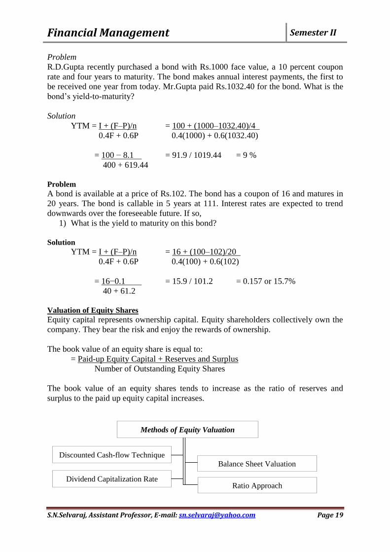
Methods of Equity Valuation

Discounted Cash-flow Technique Balance Sheet Valuation

Dividend Capitalization Rate Ratio Approach



Discounted Cash-flow Technique

The value of equity is obtained by discounting expected cash-flows to equity, i.e. the

residual cash flows after meeting all expenses, tax obligations, and interest and

principal payments, at the cost of equity, i.e. the rate of return required by equity

investors in the firm. For this valuation the following estimations should be done.

1) Estimates the future cash flows from the investments

2) Estimates a reasonable discount rate after considering the risk

3) Calculation to compute the present value of the future cash flows.

t=n

Value of Equity = ∑ CF to Equityt where, CF = Expected cash flow

t =1

(1+r)t r = Cost of Equity

For example,

Mr.Ashok is expected to receive earning per share of Rs.100 annually for 2 years.

What is its value today if cost of equity is 12%.

Solution: The present value will be as follows:

V = [CF/(1+r)1] + [CF/(1+r)

2]

= [100/(1.12)1] + [100/(1.12)

2]

= 89.28 + 80 = Rs.169.28

Balance Sheet Valuation

Analysts often look at the balance sheet of the firm to get a handle on some valuation

measures. Three measures derived from the balance sheet are: (i) book value, (ii)

liquidation value and (iii) replacement cost.

Book Value: The book value per share is simply the net worth of the company (which

is equal to paid-up equity capital plus reserves and surplus) divided by the number of

outstanding equity shares. For example, if the net worth of Samsung Limited is Rs.30

million and the number of outstanding equity shares of Samsung is 2 million, the book

value per share works out to Rs.15 (30/2).

Liquidation Value: The book value of a firm is the result of applying a set of arbitrary

accounting rules to spread the acquisition cost of assets over a specified number of

years, whereas the market price of a stock takes account of the firm‟s value as a going

concern. In other words, the market price reflects the present value of its expected

future cash flows. It would be unusual if the market price of a stock were exactly to its

book value.

The liquidation value per share is equal to:

= Value realized from liquidating all the assets of the firm – Amount to be paid

to all the creditors and preference shareholders

Number of outstanding equity shares



For example,

The Pioneer Industries would realize Rs.45 million from the liquidation of its assets

and pay Rs.18 million to its creditors and preference shareholders in full settlement of

their claims. If the number of outstanding equity shares of Pioneer is 1.5 million, the

liquidation value per share works out to:

= Rs.45 million – Rs.18 million = Rs.18 million

1.5 million

Dividend Capitalization Approach / Dividend Discount Models

The term dividend refers to that part of profits of a company which is distributed by

the company among its shareholders after execution of retained earnings. It is the

reward of the shareholders for investment made by them in the shares of the company.

One of the most widely used equity valuation model is Dividend Discount Model

(DDM). According to the dividend discount model, the value of an equity share is

equal to the present value of dividends expected from its ownership plus the present

value of the sale price expected when the equity share is sold.

Assumptions of Dividend Discount Model

1) The future value of dividend is known by the investor.

2) Dividends are expected to be distributed at the end of each year until infinity.

3) Dividends are the only way investors get money back from the company. This

implies that any share buyback would be ignored.

4) The implication of the second assumption is that the investor is expected to

hold the share for an infinite period; he will not sell it at any moment.

Single-Period Valuation Model

The investor expects to hold the equity share for one year. The price of the equity

share will be:

P0 = [D1/(1+r)] + [P1 /(1+r)]

Where, P0 = Current price of the equity share

D1 = Dividend expected a year hence

P1 = Price of the share expected a year hence

r = Rate of return required on the equity share

For example,

Prestige‟s equity share is expected to provide a dividend of Rs.2.00 and fetch a price

of Rs.18.00 a year hence. What price would it sell for now if investors‟ required rate

of return is 12 percent?

The current price will be:

P0 = [D1/(1+r)] + [P1 /(1+r)]

= [2.00/(1.12)] + [18.00/(1.12)]

= 1.79 + 16.07

= Rs.17.86



Multi-Period Valuation Model

Single period framework is the basics of equity share valuation, the more realistic and

also the more complex, is in the case of multi-period evaluation. In multi-period

valuation equity shares have no maturity period, they may be expected to bring a

dividend stream of infinite duration.

Hence the value of an equity share may be put as:

P0 = [D1/(1+r)] + [D2 /(1+r)2] + . . . . . . + [D∞/(1+r)

∞]



D2 = Dividend expected two year hence

D∞ = Dividend expected at the end of infinity

r = Expected return

When it is applicable to finite horizon and plans to hold it for n years and sell it

thereafter for a price of Pn. Then the value of the equity will be calculated as:

P0 = [D1/(1+r)] + [D2 /(1+r)2] + . . . . . . + [Dn/(1+r)

n] + [Pn /(1+r)

n]

Constant Growth Model (Gordon Model)

One of the most popular dividend discount models, called the Gordon model as it was

originally proposed by Myron J Gorden assumes that the dividend per share grows at a

constant rate (g). The value of a share, under this assumption is:

P0 = [D1/(1+r)] + [D1(1+g) /(1+r)2] + . . . . . . + [D1/(1+g)

n /(1+r)

n+1]

P0 = [D1/(r−g)]

For example,

Ramesh Engineering Limited is expected to grow at the rate of 6 percent per annum.

The dividend expected on Ramesh‟s equity share a year hence is Rs.2.00. What price

will you put on it if your required rate of return for this share is 14 percent?

Solution: The price of Ramesh‟s equity share would be:

P0 = [D1/(r−g)] = [2.00 /(0.14−0.06)] = Rs.25.00

Super Normal Growth /Two-Stage Growth Model

The two-stage model assumes that a constant growth rate g1 exists only until

sometime T, when a different growth rate g2 is assumed to begin and continue

thereafter. The simplest extension of the constant growth model assumes that the

extraordinary growth (good or bad) will continue for a finite number of years and

thereafter the normal growth rate will prevail indefinitely.



The value of firm whose growth rate of dividends varies over time can be determined

by the following equation:

P0 = [D1/(1+g1)t]+ [Dn(1+g2)

t−n]

(1+r)t (1+r)

t


g1 = Growth rate of dividends for n years

g2 = Growth rate of dividends for years n+1 and beyond


Pn = Price of the equity share at the end of year n

r = Rate of return

P0= D1 /(1+g1)t + Dn+1 1/(1+r)

n

(1+r)t (r−g2)

The first term on the right hand side in above equation is the present value of a

growing annuity. Its value is equal to:

D1 1−[(1+g1) /(1+r)]n

r−g1

Problem: The current dividend on an equity share of Vertigo Limited is Rs.2.00.

Vertigo is expected to enjoy an above-normal rate of 20 percent for a period of 6

years. Thereafter, the growth rate will fall and stabilize at 10 percent. Equity investors

require a return of 15 percent. What is the intrinsic value of the equity share of

Vertigo?

Solution: The inputs required for applying the two-stage model are:

g1 = 20 percent; g2 = 10 percent; n = 6 years; r = 15%

D1 = D0(1+g1) = Rs.2(1.20) = Rs.2.40

Step1: Calculation the present value of dividends for the first 6 years with growth rate

at 20 percent.[D0(1+g1)t] / (1+k)

t

Year

Dividend D0(1+g1)t

Rs.2(1+0.20)t

Rate of Return

r = 0.15

Present Value

(A) × (B)

(A) (B) (C)

0 2.00 0 0

1 2.40 0.870 2.088

2 2.88 0.756 2.177

3 3.456 0.658 2.27

4 4.147 0.572 2.37

5 4.976 0.497 2.47

6 5.972 0.432 2.58

13.955



Step2: Calculation of dividend after 6 years with constant growth rate at 10 percent.

Dividend in 7th

year D7 = D6(1+g2) = Rs.5.972(1+0.10)

= Rs.6.57

Price of the share at the end of 6th

year

P6 = D7/(r−g2) = 6.57 / 0.15−0.10 = Rs.131.40

Step3: Calculation of present value of the share by discounting the price of the share

at the end of 6th

year by the required rate of return, i.e. r (r=15%).

P0 = P6 × [1 /(1+r)6]

P0 = 131.40 × [1 /(1+0.15)6]

= 131.40 × PVIF15%,6yrs

= 131.40 × 0.432

= 56.76

Present value per share equals the present value of dividend for the six years and the

present value of the share price at the end of 6th

year.

Present value per share = 13.955 + 56.76 = 70.72

Zero Growth Model

The most basic of all the DDMs is the zero growth models. This model assumes that

dividend will be constant over time, so that growth is zero and that the investor‟s

required rate of return is constant. This model is:

P0 = [D /(1+r)] + [D /(1+r)] + ….. + [D /(1+r)] + [D /(1+r)∞]

Above equation can be simplified as:

P0 = D/r

Problem

There are about 10 crore shares outstanding of a company‟s 8 percent preferred

capital. The par value is Rs.100 and the dividend is paid every quarter. Assuming that

the discount rate is 10 percent, compute the value of the share.

Solution: Dividend payment every quarter will be 100×0.08/4 = Rs.2. The annual

dividend can be computed using the real rate of dividend. Nominal rate is 8 percent

per annum. The real rate of dividend payment every year will be:

[1+ (r/4)^4 – 1] = 1.0824 – 1 = 0.0824 or 8.24%

The annual dividend to be paid on the preference shares is Rs.8.24.

Using the zero-growth model, dividend payment will be divided by the discount rate,

assuming an indefinite flow of Rs.8.24. the value of the preference shares will be:

108.1 /1.10 = Rs.98.40



H–Model

A variant of the two-stage model is the H-model in which growth begins at a high rate

and declines linearly over time to reach the normal rate at the end.

The H-Model of equity valuation is based on the following assumptions:

1) While the current dividend growth rate, ga, is greater than gn, the normal long-

run growth rate, the growth rate declines linearly for 2H years.

2) After 2H years the growth rate becomes gn.

3) At H years the growth rate is exactly halfway between ga and gn.

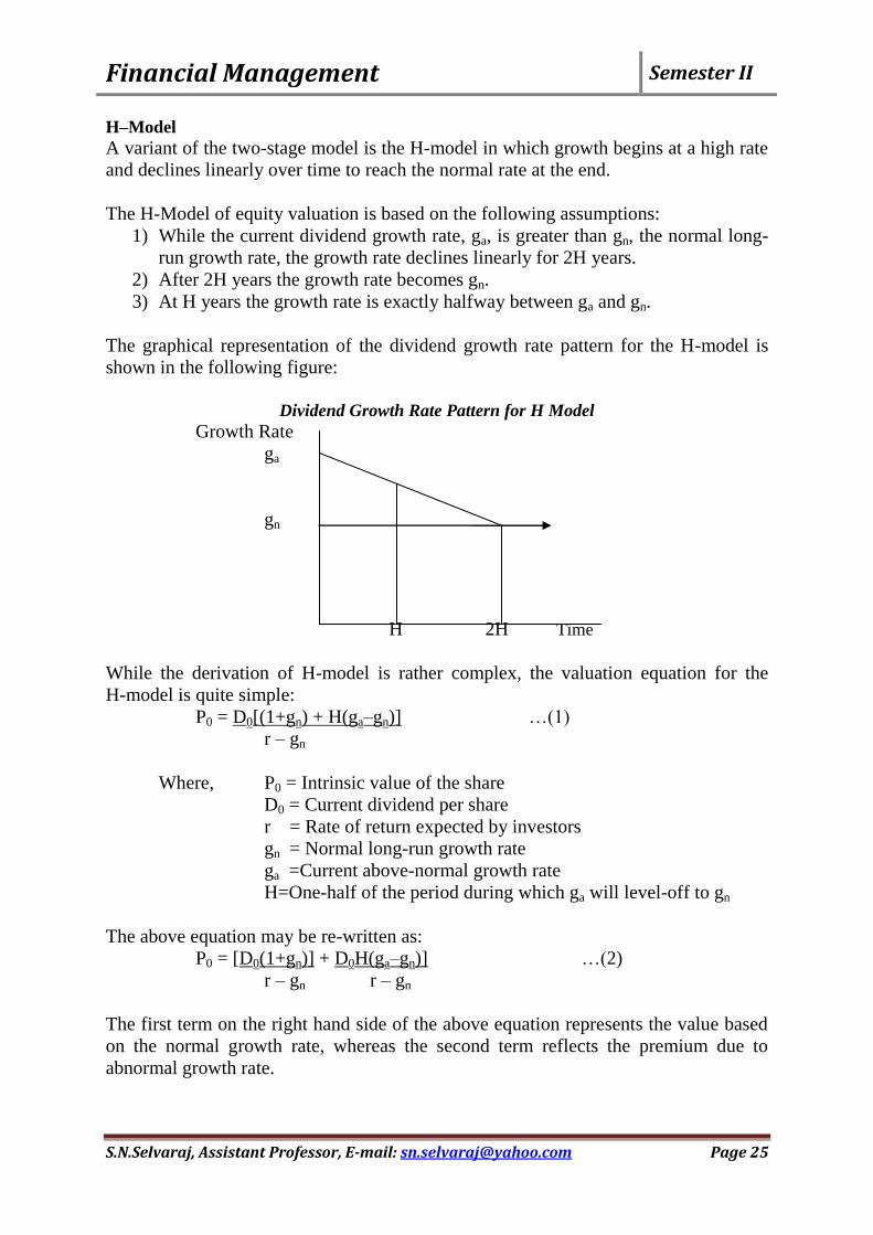
The graphical representation of the dividend growth rate pattern for the H-model is

shown in the following figure:

Dividend Growth Rate Pattern for H Model

Growth Rate

ga

gn

H 2H Time

While the derivation of H-model is rather complex, the valuation equation for the

H-model is quite simple:

P0 = D0[(1+gn) + H(ga–gn)] …(1)

r – gn

Where, P0 = Intrinsic value of the share

D0 = Current dividend per share

r = Rate of return expected by investors

gn = Normal long-run growth rate

ga =Current above-normal growth rate

H=One-half of the period during which ga will level-off to gn

The above equation may be re-written as:

P0 = [D0(1+gn)] + D0H(ga–gn)] …(2)

r – gn r – gn

The first term on the right hand side of the above equation represents the value based

on the normal growth rate, whereas the second term reflects the premium due to

abnormal growth rate.



Problem

The current dividend on an equity-share of International Computers Limited is

Rs.3.00. The present growth rate is 50 percent. However, this will decline linearly

over a period of 10 years and then stabilize at 12 percent. What is the intrinsic value

per share of the company, it investors require a return of 16 percent?

Solution: The inputs required for applying H-model are:

D0 = Rs.3.00; ga = 50 percent; H = 5 years; gn= 12 percent; r = 16 percent

Putting these inputs in the H-model, the intrinsic value estimate as follows:

P0 = [D0(1+gn)] + D0H(ga–gn)]

r – gn r – gn

= 3.00[(1.12) + 5(0.50 – 0.12)] = 9.06 = Rs.226.50

0.16 – 0.12 0.04

Ratio Approach

The ratio approach to the valuation of equity shares includes Price-Earnings Ratios

and Earnings Multiplier Approach.

Price-Earnings Ratios:Despite the inherent sensibility of dividend discount models,

many security analysts follow a much simpler procedure to value equity by using

Price-Earnings (P/E) ratios. The P/E ratio indicates the price being paid for each rupee

of a firm‟s earnings.

The ratio of equity is equal to its current market price divided by some measure of

earnings per share, that is:

P/E Ratio = Market Price / Earnings per share

Earnings Multiplier Approach:The P/E ratio is a commonly utilized tool for equity

analysts. The Earnings Multiplier Approach is a means to forecast future earnings of a

company and consequently the estimated P/E ratio. To calculate the earnings

multiplier, multiply the aggregate earnings by the P/E to market value.

To derive the P/E estimate, the dividend discount model is used as:

(P0)/(E1) = (D1/E1) /(Ke – g)

Where, P0 = Price of security

E1 = Project earnings in the next year

D1 = Dividend estimated for the next year

Ke = Required return on equity capital

g = Growth rate

Earnings Multiplier = P/E ratio × Aggregate Earnings



Valuation of Preference Shares

It is form of equity instrument. It represents a hybrid in the sense that it is an equity

interest with certain features resembling debt. Preference shares have preference rights

over common stock with respect to dividends and liquidation process. In other words,

it has priority when dividend payments and liquidating distributions are made.

If desired, dividends can accrue at a pre-established rate and can be paid on a

cumulative basis when cash flow permits. Also, preference shares may be voting or

non-voting or entitled to certain redemption rights.

Present Value of Preference Shares

Since dividends from preference shares are assumed to be perpetual payments, the

intrinsic value of shares will be estimated from the following equation valid for

perpetual in general:

Vp = [C/(1+Kp)] + [C/(1+Kp)2] + ………

Where, Vp = the value of a perpetuity today

C = the constant annual payment to be received

Kp = the required rate of return appropriate for the perpetuity

Substitute only preference divided (D) for “C” and the appropriate required return

(Kps) for „Kp‟ to obtain the following equation for valuing preference shares:

Vp = D/Kps

It is noted that „D‟ is perpetuity and is known and fixed forever.

Problem

What is the value of a preference share where the dividend rate is 18% on Rs.100 par

value? The appropriate discount rate for a stock of this risk level is 15%.

Solution: Vp = (0.18 × Rs.100) /0.15 = Rs.18/0.15 = Rs.120

Problem

The preference shares of RKV Group are selling for Rs.47.50 per share and pay a

dividend of Rs.2.35 in dividends. What is the expected rate of return if we purchase

the security at market price?

Solution: Expected rate of return = Dividend / Market price

= Rs.2.35 / 47.50 = 4.95%

OPTION VALUATION

Options are derivatives contracts that give the buyer the right to buy or sell an

underlying asset at a certain price within a specified time period. Selling or buying

options involves two parties, namely a buyer and a seller. The strategy of selling

options is popular mostly with traders who are capable of meaning the element of risk

that is inherent in such transactions.



An option is a type of a contract between two parties where one person grants the

other person the right, but not the obligation, to buy a specific asset at a specific price

within a specific time period. Alternatively, the contract may grant the other party the

right, but not the obligation, to sell a specific asset at a specific price within a specific

time period.

Types of Options

There are two types of options: (i) Call Options and (ii) Put Options. Before

commodity options were banned in India in 1952, the same two types of options were

traded as “teji” (call) and “mandi” (put) in the security market.

In Call Option, the option buyer has the right, but not the obligation, to buy the

commodity at the predetermined price.For example, A enters into a contract with B

whereby A has the right to purchase 100 ounces of gold from B for Rs.400 per ounce

at any time prior to August 1. For granting this option A pays B an option premium of

Rs.5 per ounce. This is a call option.

In Put Option, the option buyer has the right, but not the obligation, to sell the

commodity at a specified price. For example, X enters into a contract with Y whereby

X has the right to sell 100 ounces of gold from Yat a price of Rs.400 at any time

before August 1. For granting this option X pays YRs.6 per ounce as premium. This is

a put option.

Option Terminology

1) Index Options: These options have the index as the underlying. Some options

are European while others are American. Like index futures contracts, index

options contracts are also cash settled.

2) Stock Options: Stock options are options on individual stocks. A contract gives

the holder the right to buy or sell shares at the specified price.

3) Buyer of an Option: The buyer of an option is the one who by paying the option

premium buys the right but not the obligation to exercise his option on the

seller/writer.

4) Writer of an Option: the writer of a call/put option is the one who receives the

option premium and is thereby obliged to sell/buy the asset if the buyer

exercises his right.

5) Expiration Date: The date specified in the option contract is known as the

expiration date, the exercise date, the strike date or the maturity.

6) Strike Price: The price specified in the options contract is known as the strike

price or the exercise price.

7) In-the-Money: An ITMoption is an option that would lead to a positive cash

flow to the holder if it were exercised immediately. A call option on the index

is said to be in-the-money when the current index stands at a level higher than

the strike price (i.e. spot price > strike piece). In case of put option, the put is

ITM if the index is below the strike price.



8) At-the-Money: An ATM option is an option that would lead to zero cash flow if

it were exercised immediately. An option on the index is at-the-money when

the current index equals the strike price (i.e. spot price = strike piece).

9) Out-of-the-Money: an OTM option is an option that would lead to a negative

cash flow if it were exercised immediately. A call option on the index is out-of-

the-money when the current index stands at a level lesser than the strike price

(i.e. spot price < strike piece). In case of put option, the put is OTM if the index

is above the strike price.

Problem

Jerry House paid a premium of Rs.4 per share for one 6-month call option contract

(total of Rs.400 for 100 shares) of the Mahony Corporation. At the time of the

purchase, Mahony stock was selling for Rs.56 per share and the exercise price of the

call option was Rs.55.

i) Determine Jerry‟s profit or loss if the price of Mahony‟ stock is Rs.54 when

the option is exercised?

ii) What is Jerry‟s profit or loss if the Mahony‟s stock is Rs.62 when the

option is exercised?

iii) Ignore taxes and transaction cost.

Solution

i) Cost of call = (Rs.4 premium)×100 = Rs.400

Ending value = (−Rs.400 cost) + (0 gain) = Rs.400 loss

The option was worthless because the stock‟s price is less than the exercise

price at maturity.

ii) Cost of call = 400

Ending value = −Rs.400 + (Rs.62−55)×100

= −400 + 700 = Rs.300 gain

American Options & European Options

American Options are options that can be exercised at any time up to the expiration

date. Most exchange traded options are American. Most of the options that trade on

organized exchanges are American options. For example, the Chicago Board Options

Exchange (CBOE) trades American options, primarily on stocks and stock indexes

like the S&P 100 and the S&P 500. European options traded from the mid-1980s

through 1992 on the American Stock Exchange and are often traded in the over-the-

counter market as well. The American Stock Exchange reintroduced them in the late

1990s.

For example, On March 1, the price of copper is $1800 per tonne. „A‟ apprehends a

rise in price and buys an American option on June Copper (maturity date June 15) at a

strike price of $1800. The prices subsequently are as follows:

May 15: $2100

June 15: $1700



As the option is an American option, „A‟ exercises it on May 15 and sells the copper

at a profit of $300 per tonne.

European Options are options that can be exercised only on the expiration date itself.

European options are easier to analyze than American options and properties of an

American option are frequently deduced from those of its European counter-part.

European options are easier to value than American options because the analyst‟s need

only be concerned about their value at one future date.

Both European and American options have the same value. Because of their relative

simplicity and because the understanding of European option, valuation is often the

springboard to understanding the process of valuing the more popular American

options.

Factors Determining Option Price

In purchasing an option the amount the buyer pays for the option privilege is called

the premium, or sometimes the option money. In most option transactions the contract

price is the stock market price prevailing at the time the option is written and the

premium becomes the variable over which buyer and seller bargain.

1) Volatility:

2) Expiration Date: 3) Striking Prices:

4) Stock Price:

5) Dividends:

6) Interest Rates: Black-Scholes Option Pricing Model (BSOPM)

Option pricing theory also called Black-Scholes theory or derivatives pricing theory

traces its roots to Bachelier who invented Brownian motion to model options on

French government bonds. This work anticipated Einsten‟s independent use of the

Brownian motion in physics by five years. The Black-Scholes model is used to

calculated a theoretical call price (ignoring dividends paid during the life of the

option) using the five key determinants of an option‟s price; stock price, strike price,

volatility, time to expiration and short-term (risk-free) interest rate.

The original formula for calculating the theoretical Option Price (OP) is as follows:

C = SN(d1) – Ee−rt

N(d2)

Where, d1 = In[S/E] + [r+(1/2)σ2]tand d2 = In[S/E] + [r−(1/2)σ

2]t

σ√t σ√t

The variables are:

S = Stock price

E = Strike price

t = Time remaining until expiration

r = Risk free interest rate

σ = Annual volatility of stock price (standard deviation)



In = Natural logarithm

e = Exponential function

N = Standard normal cumulative distribution function

The Black-Scholes model gives theoretical value for European put and call options on

non-dividend paying stocks. The key argument is that traders could riskless hedge a

long options position with a short position in the stock and continuously adjust the

hedge ratio (the delta value – one of the option sensitivities known as „greeks”) as

needed. Assuming that the stock price follows a random walk, and using the methods

of stochastic calculus, a price for the option can be calculated where there is no

arbitrage profit.

Assumptions of Black and Scholes Model

1) Stock Pays no Dividends during the Option‟s Life

2) European Exercise Terms are Used

3) Markets are Efficient

4) No Commissions are Charged

5) Interest Rates remain Constant and Known

6) Returns are Long-normally Distributed

Advantages of Black & Scholes Model

The main advantage of the Black & Scholes model is speed.

It helps to calculate a very large number of option prices in a very short time.

Disadvantages of Black & Scholes Model

It cannot be used to accurately price options with an American-style exercise.

It is limited to exercise only to the European options which can only be

exercised at expiration.

Text Books

1. M.Y.Khan and P.K.Jain, “Financial Management” Tata McGraw Hill, 6th

Edition, 2011.

2. I.M.Pandey, “Financial Management” Vikas Publishing House Pvt. Ltd., 10th

Education 2012. References

1. AswatDamodaran, Corporate Finance Theory and Practice, John Wiley &

Sons, 2011.

2. James C Vanhorne, Fundamentals of Financial Management, PHI Learning,

11th

Edition, 2012.

3. Brigham Ehrhardt, Financial Management Theory and Practice, Cengage

Learning, 12th

Edition, 2010.

4. Prasanna Chandra, Financial Management, Tata McGraw Hill, 9th

Edition,

2012.

5. Srivatsava, Mishra, Financial Management, Oxford University Press, 2011.

Date post:	14-Jul-2015
Category:	Education
Upload:	snskpm1966
View:	262 times
Download:	3 times