Back to the Basics in Banking? A Micro-Analysis of …wps-feb.ugent.be/Papers/wp_09_579.pdf · Back...

FACULTEIT ECONOMIE EN BEDRIJFSKUNDE

TWEEKERKENSTRAAT 2 B-9000 GENT

Tel. : 32 - (0)9 – 264.34.61 Fax. : 32 - (0)9 – 264.35.92

WORKING PAPER

Back to the Basics in Banking? A Micro-Analysis of Banking System Stability.

Olivier De Jonghe

April 2009

2009/579

Forthcoming in Journal of Financial Intermediation.

D/2009/7012/31

Back to the Basics in Banking? A Micro-Analysis of Banking

System Stability.�

Olivier De Jonghey

Ghent University

Abstract

This paper analyzes the relationship between banks' divergent strategies toward specialization and di-

versi�cation of �nancial activities and their ability to withstand a banking sector crash. We �rst generate

market-based measures of banks' systemic risk exposures using extreme value analysis. Systemic banking

risk is measured as the tail beta, which equals the probability of a sharp decline in a bank's stock price con-

ditional on a crash in a banking index. Subsequently, the impact of (the correlation between) interest income

and the components of non-interest income on this risk measure is assessed. The heterogeneity in extreme

bank risk is attributed to differences in the scope of non-traditional banking activities: non-interest generating

activities increase banks' tail beta. In addition, smaller banks and better-capitalized banks are better able to

withstand extremely adverse conditions. These relationships are stronger during turbulent times compared to

normal economic conditions. Overall, diversifying �nancial activities under one umbrella institution does not

�Part of the research was undertaken while Olivier De Jonghe was an intern at the European Central Bank (Directorate Financial

Stability) and the National Bank of Belgium (Financial Stability Division). The author would like to thank the members of both departments

for helpful comments and discussions. Jan Annaert, Lieven Baele, David Brown, Bertrand Candelon, Ferre De Graeve, Hans Degryse,

Joel Houston, Ani Manakyan, Steven Ongena, Richard Rosen, Stefan Straetmans, Rudi Vander Vennet, two anonymous referees, the

editor (George G. Pennacchi) and participants in the third European Banking Symposium (Maastricht), the conference on 'Identifying

and resolving �nancial crises' organized by the Federal Reserve Bank of Cleveland and the FDIC, and the 2008 FMA meeting (Dallas)

provided helpful comments.yOlivier De Jonghe gratefully acknowledges the hospitality and �nancial support of Ente Luigi Einaudi for Monetary, Banking and

Financial Studies, Rome, during a visiting appointment as a Targeted Research Fellow, during May-July, 2008. De Jonghe is Postdoc-

toral Researcher of the Fund for Scienti�c Research - Flanders (Belgium) (F.W.O.-Vlaanderen) and a Fellow of the Belgian American

Educational Foundation (visiting the University of Florida). Email: [email protected]

improve banking system stability, which may explain why �nancial conglomerates trade at a discount.

Keywords: diversi�cation, non-interest income, �nancial conglomerates, banking stability, extreme value analysis, tail

risk.

JEL: G12, G21, G28.

2

1 Introduction

The subprime crisis reminds us that, notwithstanding a period of disintermediation, the banking sector remains

a particularly important sector for the stability of the �nancial system. Moreover, disruptions in the smooth

functioning of the banking industry tend to exacerbate overall �uctuations in output. Consequently, banking

crises are associated with signi�cant output losses. It follows that preserving banking sector stability is of

the utmost importance to banking supervisors. That is, regulators are especially interested in the frequency

and magnitude of extreme shocks to the system which threaten the smooth functioning (and ultimately the

continuity) of the banking system. Banking sector supervisors and central banks' main interest is to maintain

and protect the value of their portfolio of banks in times of market stress. Thus it is interesting to study the

factors contributing to the riskiness of the portfolio.

In this spirit, an extensive literature1 reviews banking crises around the world, examining the developments

leading up to the crises as well as policy responses. Initial research focussed on macro-prudential supervision

and investigates the relationships between macro-economic conditions and banking system stability (see e.g.

Demirgüc-Kunt and Detragiache, 1998; Eichengreen and Rose, 1998). Subsequently, attention shifted towards

the impact of the regulatory and institutional environment on banking crises (see e.g. Barth, Caprio and Levine,

2004; Beck, Demirgüc-Kunt and Levine, 2006; Demirgüc-Kunt and Detragiache, 2002; Houston, Lin, Lin and

Ma, 2008). However, not all banks need to contribute equally to the risk pro�le of the supervisor's portfolio

and the stability of the banking system. Nevertheless, research that zooms in at the micro-level and aims to

identify bank-speci�c characteristics of banking system stability is limited. Moreover, almost all evidence is

based on analyzing the determinants of outright bank failures in the US (see e.g. Gonzalez-Hermosillo, 1999,

and the references in Appendix 1 of that paper; and Wheelock and Wilson, 2000).

This paper investigates why some banks are better able to shelter themselves from the storm by analyzing

the bank-speci�c determinants of individual banks' contribution to systemic banking risk. Our research con-

tributes to the banking literature in a number of ways. First, a crucial addition to the analysis is our measure

of individual bank risk during extremely adverse economic conditions. More precisely, we estimate tail betas

(Hartmann, Straetmans and de Vries, 2006 and Straetmans, Verschoor and Wolff, 2008) rather than analyzing

actual defaults. Tail beta measures the probability of a crash in a bank's stock conditional on a crash in a Euro-1Cihak and Schaeck (2007) provide an excellent overview of the empirical literature on the determinants of banking system stability.

3

pean banking sector stock price index. The choice of this measure is driven by two empirical stylized facts on

banking panics. Historically, banking panics occurred when depositors initiated a bank run. In more recent pe-

riods, banks face a stronger disciplining role by stock market participants. As a consequence, equity and bond

market signals are good leading indicators of bank fragility (Gropp, Vesala and Vulpes, 2006). Therefore, we

employ a market-based measure. In addition, Gorton (1988) and Kaminsky and Reinhart (1999) document that

most banking panics have been related to systemic and macroeconomic �uctuations rather than 'mass hysteria'

or self-ful�lling prophecies. Therefore, we look at the conditional rather than the unconditional probability of

a crash in a bank's stock price. By measuring the tail beta for all listed European banks over different time

periods we document the presence of substantial cross-sectional heterogeneity and time variation in the tail

betas of European banks.

Second, we contribute to the debate on the scope of �nancial �rms by analyzing the impact of revenue

diversity on banking system stability. In recent years, one of the major developments in the banking industry

has been the dismantling of the legal barriers to the integration of distinct �nancial services and the subsequent

emergence of �nancial conglomerates. In Europe, the Second banking Directive of 1989 allowed banks to

combine banking, insurance and other �nancial services under a single corporate umbrella. Similar deregulat-

ing initiatives took place in the US by means of the Gramm-Leach-Bliley Act of 1999. These deregulations

resulted in an expansion in the variety of activities and �nancial transactions in which banks engaged. Most of

the existing research addressing the issue of the economies of scope in �nancial corporations takes an industrial

organization approach and analyzes whether �nancial conglomerates create or destroy value (see e.g. Laeven

and Levine, 2007; Schmid and Walter, 2009). Recent studies also analyze whether functional diversi�cation

reduces bank risk by investigating functional diversi�cation from a portfolio perspective (see e.g. Baele, De

Jonghe and Vander Vennet, 2007; Stiroh, 2006). We contribute to the empirical literature on revenue diversity

of �nancial corporations by addressing a third perspective, that of �nancial stability. Our results establish that

the shift to non-traditional banking activities, which generate commission, trading and other non-interest in-

come, increases banks' tail betas and thus reduces banking system stability. Interest income is less risky than

all other revenue streams. Other indicators of bank specialization in traditional intermediation, such as a higher

interest margin or higher loans-to-asset ratio, corroborate the �nding that traditional banking activities result in

lower systemic banking risk. This questions the usefulness of �nancial conglomeration as a risk diversi�cation

4

device, at least in times of stock market turmoil. The results are consistent with the theoretical predictions of

Wagner (2008) that even though diversi�cation may reduce each bank's probability of default, it makes sys-

temic crises more likely. However, we also document that the extent to which shocks to the various income

shares are correlated matters for overall and extreme bank risk.

Third, we attribute a substantial degree of the time and cross-sectional heterogeneity to other bank-speci�c

characteristics. The variables we include capture the constituents of the CAMEL rating methodology, i.e.

Capital adequacy, Asset quality, Management quality, Earnings, Liquidity. Appendix 1 of Gonzalez-Hermosillo

(1999) provides an interesting overview of the variables used in selected empirical studies on US bank failures

and also classi�es these according to the constituents of the CAMEL rating. Wheelock and Wilson (2000)

use similar variables to analyze why banks disappear. Smaller banks and well-capitalized banks contribute

signi�cantly to a safer banking system. In terms of economic impact, the latter results are somewhat larger

than the gains from focussing on the traditional intermediation activities.

Finally, we show that the focus on extreme bank risk and banking system stability provides insights supple-

mentary to the existing evidence on banks' riskiness in normal economic conditions. The information content

of tail betas differs from measures focussing on central dependence or composite risk measures (such as long-

term debt ratings or equity return volatility). We obtain, for instance, that higher capital buffers work best when

they are needed the most, i.e. in times of stress.

The following section reviews relevant literature on banking system stability, the risk-taking incentives

of �nancial conglomerates and the impact of revenue diversity on bank risk. In Section 3, we discuss the

sample composition. The next section describes the methodology to measure banks' tail betas. The subsequent

section, Section 5, is divided into three subsections. The �rst subsection introduces the results for the drivers of

heterogeneity in systemic banking risk. In a panel set-up, we relate the tail betas to different types of �nancial

revenues and other bank-speci�c variables. While these issues are always important, the magnitude of the

recent �nancial crisis renews interest in these questions. The second subsection documents that the information

content of the tail beta differs signi�cantly from the information contained in central dependence measures

(such as the traditional OLS beta between bank stock returns and returns on a banking index). Subsection 5.3.

deals with re�nements on the panel data set-up and robustness of the baseline regression. We show that the

results are not driven by reverse causality or particular events (such as M&As, IPOs, delisting or banking crises)

5

that may create a sample selection bias. Furthermore, we scrutinize the impact of composite risk measures (such

as ratings or volatility) on the tail beta as well as control for the stability of the results in subsamples based on

bank size. Section 6 concludes with policy implications.

2 Literature review

2.1 Banking regulation and systemic banking risk: selected literature

Systemic banking risk can be de�ned as an event that affects a considerable number of �nancial institutions

in a strong sense, thereby severely impairing the general well-functioning of the �nancial system. This well-

functioning of the �nancial system relates to the effectiveness and ef�ciency with which savings are channelled

into the real investments promising the highest returns (de Bandt and Hartmann, 2002). Hence, historically,

most of the banking regulation that was put in place was designed to reduce systemic risk.

In many countries, one of the most important measures to reduce systemic risk is currently capital regulation

in the form of the Basel agreements. In all standard models of banking, high capital levels are associated

with a lower bankruptcy risk (Santos, 2001). However, current regulation is based only on a bank's own risk

and ignores the externalities of the bank's actions. Acharya (2009) shows that such regulation may leave the

collective risk-shifting incentive unattended, and can, in fact, accentuate systemic risk. He concludes that

prudential supervision should thus operate at a collective level, and regulate each bank such that the capital

adequacy requirement is increasing in the individual risk of each bank as well as in the correlation of banks'

risks.

Next to capital regulation, deposit insurance schemes are put in place to prevent bank runs by depositors.

Explicit deposit insurance has become increasingly popular, and a growing number of depositors around the

world are now sheltered from the risk of bank failure. However, according to the �ndings of Demirgüc-Kunt

and Detragiache (2002), explicit deposit insurance may also be detrimental to bank stability, the more so

where bank interest rates have been deregulated and where the institutional environment is weak. Hence,

where institutions are good, opportunities for moral hazard are more limited, and more effective regulation and

prudential supervision better offset the adverse incentives created by deposit insurance.

Regulation often tends to increase after a severe and systemic crisis. In the aftermath of the stock market6

crash of 1929 and the Great Depression, the Banking Act of 1933, better known as the Glass-Steagall Act, sep-

arated the activities of commercial banks and investment banks. The idea behind it was twofold: �rst, diffuse

excessive concentration of �nancial power in a limited number of large institutions, and second, prevent unso-

phisticated investors from being sold risky investments. However, over time there has been some deregulation.

The Glass-Steagall Act was abolished by a series of laws from the 1980s (relaxation of branching restrictions)

until the late 1990s (culminating in the Gramm-Leach-Bliley in 1999). The main effect of this deregulation

was permitting American banks to do what European banks had long been allowed to do, the combination

of various types of �nancial activities under one umbrella institution (since the Second Banking Directive of

1989). However, there is little theoretical or empirical guidance as to whether revenue diversity helps or harms

banking system stability.

2.2 Revenue diversity and bank risk: selected literature

Most of the theoretical and empirical literature that studies the effects of combining different activities un-

der one umbrella institution focus on the performance component. This focus on the bene�t or discount that

conglomeration creates can be justi�ed for non-�nancial corporations; however, the risk aspect is at least as

important, if not more so, for �nancial corporations. Unfortunately, little theoretical guidance exists on the

impact of diversi�ed revenue streams on the risk-taking behavior of �nancial institutions. The main sources

of the potential risk-reducing effects of revenue diversity are the less than perfect correlations between differ-

ent activities (Dewatripont and Mitchell, 2005) and the organizational structure of the conglomerate (Freixas,

Loranth and Morrison, 2007). Wagner (2008) documents that diversi�cation at �nancial institutions entails

a trade-off. Functional diversi�cation may reduce idiosyncratic risk, but it also makes systemic crises more

likely.

A number of authors empirically identify the impact of combining different �nancial activities on a bank's

risk pro�le during normal economic conditions. Evidence for the US2 documents that in the 1990s securities

and insurance activities both had the potential to decrease conglomerate risk, but the effect largely depends

on the type of diversifying activities that bank holding companies undertake. Expanding banks' activities may2Despite the fact that the scope for functional diversi�cation has been deregulated earlier and more completely in Europe, most of the

empirical evidence is based on US data.

7

reduce risk, with the main risk-reduction gains arising from insurance rather than securities activities (see

e.g. Kwan and Laderman, 1999 and Saunders and Walter, 1994). Moreover, diversi�cation of non-traditional

banking activities leads to a lower cost of debt (Deng, Elyasani and Mao, 2007). However, these arguments are

contradicted somewhat by more recent �ndings (DeYoung and Roland, 2001; Stiroh, 2004a; Stiroh, 2004b and

Stiroh and Rumble, 2006). For the US, studies using accounting data suggest that an increased reliance on non-

interest income raises the volatility of accounting pro�ts without signi�cantly raising average pro�ts. There

are only small diversi�cation bene�ts for Bank Holding Companies and the gains are offset by the increased

exposure to more volatile non-interest income activities for more diversi�ed US banks. Results based on US

equity data (Stiroh, 2006) arrive at a similar conclusion. For a sample of US banks over the period 1997-2004,

no signi�cant link between non-interest income exposure and average returns across banks can be established.

On the other hand, the volatility of market returns is signi�cantly and positively affected by the reliance on

non-interest income.

European banks that have moved into non-interest income activities present a higher level of risk than banks

which mainly perform traditional intermediation activities (Mercieca, Schaeck and Wolfe, 2007). Moreover,

risk is mainly positively correlated with the share of fee-based activities but not with trading activities (Lepetit,

Nys, Rous and Tarazi, 2008). Recent research linking the effect of diversi�cation to market-based measures

of performance and riskiness (and the risk/return trade-off) �nds that banks with a higher share of non-interest

income in total income are perceived to perform better in the long run (Baele et al., 2007). However, this better

performance is offset by higher systematic risk. Diversi�cation of revenue streams from different �nancial

activities increases the systematic risk of banks i.e., the stock prices of diversi�ed banks are more sensitive

to normal �uctuations in a general stock market index than non-diversi�ed banks. Finally, using a worldwide

sample, de Nicolo, Barthlomew, Zaman and Zephirin (2004) report that conglomerates exhibit a higher level

of risk-taking than non-conglomerates.

All of this evidence addresses normal economic conditions, however, regulators are especially interested in

the frequency and magnitude of extreme events. To the best of our knowledge, only Schoenmaker, Slijkerman

and de Vries (2005) take this perspective and analyze the dependence between the downside risk of European

banks and insurers. However, their analysis is limited to ten banks and ten insurers. Schoenmaker et al.

(2005) investigate whether the extreme risk pro�le of arti�cially mixed pairs differs from the risk pro�le of

8

bank-bank combinations. They argue that if the risk pro�le of both sectors is different, this should create risk

diversi�cation possibilities for �nancial conglomerates and increase �nancial sector stability.

Most of the available evidence identi�es relationships between functional diversi�cation and bank risk in

normal economic conditions. However, it is not clear how diversi�ed �nancial institutions will behave in

adverse economic situations and what the overall impact of revenue diversi�cation on banking sector stability

will be under these circumstances. This paper attempts to �ll this void.

3 The sample

Since the purpose of the analysis is to investigate how diversity in bank revenue affects European banks'

extreme systemic and systematic risk, we employ both accounting data and stock price information. We extract

information from two data sources. For balance sheet and income statement data, we rely on the Bankscope

database, which provides comparable information across countries. Bankscope does not provide stock price

information on a daily basis; hence we use Datastream to obtain information on daily stock returns and market

capitalization. We match both datasets on the basis of the ISIN-identi�er (an identi�cation system similar to

the CUSIP number in the US and Canada) for the listed banks. Unfortunately, Bankscope does not provide the

ISIN-number for delisted banks. For the delisted banks, we match the information from the two datasets using

information on some basic accounting data (e.g. total assets, equity,... which are also provided by Datastream).

In a similar fashion, we verify the matching of the listed banks.

We carry out the analysis for the banks that have their headquarters in one of the countries of the European

Union (before enlargement, i.e. with 15 member states). Our sample consists of both commercial banks and

bank holding companies. The sample period is to a large extent �xed by the availability of comparable data

over time. While Bankscope contains information from 1987 onwards, the coverage is only substantial from

the early nineties. Therefore, we perform the analysis on the sample period 1992-2007. The time span of the

sample ensures that it contains periods with different business cycle conditions and stock market conditions.

We perform a number of selection criteria. First, we only include banks for which we can obtain at least

six consecutive years of accounting and stock market information. This restriction is imposed because we use

extreme value analysis to model extreme bank risk. In extreme value analysis, large samples are needed since

only a fraction of the information is used in the estimations. Six consecutive years of daily stock prices yield at9

least 1500 observations, a sample size that is feasible to apply extreme value analysis, though close to the lower

bound3 of the existing applications in �nance. Second, following common practice in the �nance literature, we

impose a liquidity criterion on the stock returns. The rationale is that infrequently traded stocks may not absorb

information accurately. We measure liquidity by the number of daily returns that are zero. However, in this

analysis we can be rather mild on the imposed liquidity criterion. We only disregard stock if more than 60%

of the daily returns are zero returns. Hence, we assume that although these bank stocks are very illiquid, their

non-zero returns most likely re�ect important, extreme events that are informative for our purposes. Moreover,

their zero returns will not affect our estimates of extreme risk, since the tail of the distribution will still contain

the extreme movements in banks' stock prices.

Due to delistings, IPOs, and mergers and acquisitions, our dataset is unbalanced. Some banks are only listed

for six years whereas others have been operational and listed for a longer period. Comparing banks' behavior

and risk pro�le is only sensible if each bank's characteristics are measured over the same time interval. One

possibility is to consider only those banks that are active (and listed) over the entire period. However, in

this case, useful information on the other banks is neglected and may induce a selection bias. We opt for a

different approach. We measure banks' extreme systemic risk exposures over moving windows of six years.

The �rst period covers the years 1992-1997. In each subsequent subsample, we drop the observations of the

initial sample year and add a more recent year of data. Since the sample period spans 16 years, we obtain 11

rolling subsamples of six years. Hence, at each point in time, we can meaningfully compare the cross-sectional

differences in banks' risk pro�le. In general, the composition of the bank set will be different in each subperiod.

4 A stock market-based measure of bank stability

As the stock market moves, each individual asset is more or less affected. The extent to which any asset par-

ticipates in such general market moves determines that asset's systematic risk. In general, systematic risk is

measured using a �rm's beta and is computed by dividing the covariance between the �rm's stock returns and

the market return by the variance of the market returns. However, �rms' exposure to systematic risk need not be

constant over time. In particular, systematic risk exposures may vary over the business cycle or can be different

in normal times versus times of market turbulence. While the combination of correlation-based methods and3We also perform the analysis on moving subsample of 8 years. The results are very similar.

10

assuming multivariate normality may yield acceptable results for central dependence measures, there exists

abundant evidence that marginal and joint distributions of stock returns are not normally distributed, especially

in the tail area. This might be solved by modelling the tail behavior with fat-tailed distributions. However,

this requires distributional assumptions or knowledge of the underlying return processes. Choosing the wrong

probability distribution may be problematic since correlations are non-robust to changing the underlying dis-

tributional assumptions of the return processes (Embrechts, Klüppelberg, Mikosch, 1999). Moreover, many

of the multivariate distributions lead to models that are non-nested, which cannot be tested against each other.

Extreme value analysis overcomes these problems. It enables estimation of marginal and joint tail behavior

without imposing a particular distribution on the underlying returns.

In mathematical terms, we are interested in the following expression: P (X > x j Y > y). This expression

captures the conditional probability that the return on one asset,X , exceeds a certain threshold x conditional on

observing that the return on another asset, Y , exceeds y. This conditional probability re�ects the dependence

between two return series X and Y . We adopt the convention to take the negative of the return when outlining

the methodology. x and y are thresholds in the tail of the distributions, such that they correspond with situations

of large losses. In general, x and y may differ across stocks (especially in our analysis where Y is the return on

a portfolio andX is single stock), but we impose that they correspond to outcomes that are equally (un)likely to

occur. That is, the unconditional probability that an asset crashes equals p = P (X > x) = P (X > Qx(p)) =

P (Y > Qy(p)), where Qx and Qy are quantiles.

The conditional co-crash probability can be rewritten as:

P (X > Qx(p) j Y > Qy(p)) =P (X > Qx(p); Y > Qy(p))

P (Y > Qy(p))(1)

In general, X and Y can be the returns generated by any kind of asset. However, if the conditioning asset

Y is a broad market or (banking) sector portfolio, the conditional probability can be seen as a tail extension of

a regression based � obtained in classical asset pricing models. The resulting co-crash probabilities provide an

indication of extreme systematic or systemic bank risk. Hence, an asset's co-crash probability with the banking

sector (or market), P (X > Qx(p) j Y > Qy(p)), will be labelled tail-� (Straetmans et al., 2008).

To obtain the tail-�, we only need an estimate of the joint probability in the numerator. The denominator

is determined by p. We implement the approach proposed by Ledford and Tawn (1996) and closely follow11

Hartmann et al. (2006). This approach is semi-parametric and allows both for asymptotic dependence and as-

ymptotic independence4. Hence, we can avoid making (wrong) distributional assumptions on the asset returns.

This approach has recently been used in the �nance literature by Hartmann et al. (2006), Poon, Rockinger and

Tawn (2004) and Straetmans et al. (2008).

The joint probability is determined by the dependence between the two assets and their marginal distribu-

tions. In order to extract information on the (tail) dependence, we want to eliminate the impact of the different

marginal distributions. Therefore, we transform the original return series X and Y to series with a common

marginal distribution. If one transforms the different return series to series with a common marginal distrib-

ution, the impact of marginals on the joint tail probabilities is eliminated. This means that differences in the

conditional crash probabilities of banks are purely due to differences in the tail dependency of extreme returns.

The theoretical (a) and empirical (b) counterpart of transforming the stock returns to unit Pareto marginals5 are

based on the following equations:

(a) eXi = 11�F (Xi)

and (b) eXi = n+1n+1�RXi

(2)

where i = 1; :::; n and RXiis the rank order statistic of returnXi. Since eXi and eYi have the same marginal

distribution, it follows that the quantiles Qex(p) and Qey(p) now equal q = 1=p.The transformation of the return series affects the numerator of the co-crash probability as follows:

P (X > Qx(p); Y > Qy(p)) = P ( eX > q; eY > q) = P (min( eX; eY ) > q) (3)

Hence, the transformation to unit Pareto marginals reduces the estimation of the multivariate probability

to a univariate set-up. The univariate exceedance probability of the minimum series of the two stock returns,

Z = min( eX; eY ), can now be estimated using techniques that are standard in univariate extreme value analysis6.The only assumption that has to be made is that the minimum series Z = min( eX; eY ) also exhibits fat tails.

4Asymptotic dependence means that the conditional tail probability de�ned on (X;Y ) does not vanish in the bivariate tail. With

asymptotic independence, the co-exceedance probability decreases as we move further into the bivariate tail.5Other transformations are also feasible. Poon et al. (2004) transform the return series to unit Fréchet marginals. However, the estimates

have a larger bias for Fréchet distributions (Draisma, Drees, Ferreira and De Haan, 2004).6In the remainder of this section, we still use Z to refer to the return series. In our speci�c case, Z is the series created by taking

the minimum of eX and eY . Note, however, that Z may also be the return series of a single (untransformed) stock if one wants to modelunconditional tail risk.

12

Univariate tail probabilities for fat-tailed random variables can be estimated by the semi-parametric proba-

bility estimator from De Haan, Jansen, Koedijk and de Vries. (1994):

bpq = P (Z > q) = m

n

�Zn�m;nq

�b�(4)

Zn�m;n is the �tail cut-off point�, which equals the (n�m)th ascending order statistic, in a sample of size n,

of the newly created minimum series Z. The advantage of this estimator is that one can extend the crash levels

outside the domain of the observed, realized returns. Note that the tail probability estimator is conditional upon

the tail index � and a choice of the number of tail observations used, m. This tail index captures the decay in

the probability with which ever more extreme events occur (jointly). A relatively high tail index corresponds

with a relatively low probability of extreme events. The tail index � is traditionally estimated using the Hill

estimator (1975):

b�(m) =24 1m

m�1Xj=0

ln

�Zn�j;nZn�m;n

�35�1 (5)

In this equation, Zn�j;n denotes the (n � j)-th ascending order statistic from the return series Z1; :::; Zn.

The parameter m is a threshold that determines the sample fraction on which the estimation is based (i.e.

the number of extreme order statistics that are used). This parameter is crucial. If one sets m too low, too

few observations enter and determine the estimation. If one considers a largem, non-tail events may enter the

estimation. Hence, if one includes too many observations, the variance of the estimate is reduced at the expense

of a bias in the tail estimate. This results from including too many observations from the central range. With

too few observations, the bias declines but the variance of the estimate becomes too large. Asymptotically,

there exists an optimalm at which this bias-variance trade-off is minimized.

A number of methods have been proposed to select m in �nite samples. First, a widely used heuristic

procedure in small samples is to plot the tail estimator as a function of m and select m in a region where b� isstable. This procedure is usually referred to as the Hill plot method. Besides being arbitrary, this is dif�cult to

implement if one considers many stock returns. A second option is to determine the optimal sample fraction,

m, using a double bootstrap procedure (Danielsson, Haan, Peng and de Vries, 2001). However, this procedure

requires, in general, samples that are longer than the one we observe (and it requires heavy computing power).

We apply a third method which directly estimates a modi�ed Hill estimator that corrects for the bias/variance13

trade-off (Huisman, Koedijk, Kool and Palm, 2001). Huisman et al. (2001) note that the bias is a linear function

ofm and that the variance is inversely related tom. The modi�ed estimator extracts information from a range

of conventional Hill estimates that differ in the number of tail observations included. Weighted least squares is

then used to �t a linear relationship between b�(m) and m, with the weights proportional to m. The interceptof that regression yields an unbiased estimate of the tail index. Note that, by using a large number of values of

m, this bias-corrected method is designed to reduce sensitivity to the single choice of m required by the Hill

procedure. A drawback of this method is that it only provides an unbiased measure of the tail index without

specifying the optimal sample fraction m. However, this info is still needed to compute the univariate crash

probabilities bpq. Therefore, after estimating the optimal b�, we perform an automated grid search to �nd a stableregion in the Hill plot that is as close as possible to the optimal tail index. m is then taken as the midpoint from

this region.

Combining equations (1), (4), and (5) allows computing the extreme systematic risk measure, tail-�:

TAIL� =mn (Zn�m;n)

�

p1��(6)

We will estimate this tail-� for listed European banks observed over multiple time periods to get an indica-

tion of the time evolution and the cross-sectional dispersion in banks' extreme risk sensitivities. The estimated

tail betas provide insights in the dependence of events that happen with a certain probability p. In this section

and in the remainder of the paper, we model extreme events that happen with a probability of 0:04%. Given

that we are using daily data, a probability of 0:04% corresponds to a situation that occurs on average once every

10 years (= (250 � p)�1). The probability of the event obviously affects the severity. More likely events are

associated with less severe crashes. How does the level of p affect the tail-�? This depends on the estimated

tail dependence coef�cient (the tail index � of the joint tail). Asymptotic dependence (� = 1) implies that

the conditional tail probability converges to a non-zero constant. However, asymptotic independence (� > 1)

results in vanishing co-crash probabilities in the joint tail. In our sample, both asymptotic dependence and

independence are present. Hence, for the latter, the tail-� will be larger for less extreme events. For example,

setting the crash probability at p=0:001, a level corresponding to the Basel II guidelines, results in less severe

events but higher tail betas. In the remainder of the paper, we relate tail betas to bank-speci�c characteristics.

We �x p at 0:04%. Nevertheless, we also experimented with probabilities in the range of [0:004%; 0:4%], re-14

sulting in events that happen as infrequently as once every 100 years to yearly events. All reported results with

respect to the determinants of tail risk are similar (and are available upon request).

Measuring systemic banking risk: results

We are interested in assessing the extent to which individual banks are exposed to an aggregate shock, as

captured by an extreme downturn in a broad European banking sector index. For each bank stock (as well

as the bank index), we calculated daily returns as the percentage changes in the return index. All series are

expressed in local currency to prevent distortion by exchange rate �uctuations.

Before showing the estimated tail betas, we provide insight in the severity of the events that we are mod-

elling. That is, we �rst report the unconditional Value-at-Risk levels or quantiles associated with probability

p = 0:04%. Doing so, we exploit one of the main bene�ts of modelling the entire tail of the (joint) distrib-

ution. We are looking at events that happen less frequently than the observed sample length. We summarize

the �ndings on the unconditional Value-at-Risk levels in Table 1. In order to get these crash magnitudes, we

�rst estimate the tail index for each individual series using the modi�ed Hill estimator, Eq. (5). (Z is now a

simple return series.) The magnitude of the daily loss for a given probability level can then be obtained using

the inverse of Eq. (4); that is, bq = Zn�m;n � mp�n

� 1b�. Hence, lower probability events will cause an increase in

the absolute value of the crash level, whereas events that occur more frequently (at least in terms of extreme

value analysis) will lead to lower crash magnitudes.

< Insert Table 1 around here >

Table 1 consists of three panels. Panel A contains information on the extreme losses of the European

banking sector index for eleven (overlapping) time periods of six years. The �rst block of six years covers the

period 1992-1997, the last period runs from 2002 to 2007. The �rst row reports the observed maximum daily

loss in each six-year time period. The second line contains information on the estimated daily loss that happens

with a probability of 0:04%. The estimated daily return �uctuates in the range of �5:3% and �9:3%. It is

lowest (in absolute value) in the �rst period. From the second period onwards, the turbulent year 1998 enters

the moving window. The magnitude of the estimated daily crashes (as well as the observed minimum) increases

in absolute value. The relatively benign stock market conditions of 1999 and 2000 helped in mitigating the15

extreme losses. As a consequence the expected daily loss associated with an event that happens once every

10 years decreased from �9:1% to �6:5%. However, the (minimal) severity of a crash, which is expect to

occur once every ten years, increases again from 2001 onwards to reach �9:3% in 1997-2002. The periods

1997-2002 and 1998-2003 are the periods with the largest extreme banking sector risk in the sample. In the

last time period (2002-2007), we notice a drop in the observed minimum return as well as the estimated VaR of

the European banking index. Notwithstanding that the turbulent period of 2007 enters the subperiod, the effect

of dropping the returns in the year 2001 (compared to the previous period subsample) dominates. Note that in

all but two periods, the estimated daily crash is worse than the observed minimal daily return. This is due to

looking at events that are less frequent than the moving window of six years.

Panel B contains information on the time evolution as well as the cross-sectional dispersion in the daily

losses of European bank stock returns that happen with a probability of 0:04%. The rows in panel B provide

information on the variation in the Value-at-Risk across banks at each time span we consider. We report several

percentiles as well as the mean and the standard deviation. The last row contains the number of banks we

observe in that particular period of 6 years. Again, we report the results in eleven columns, one for each

moving time frame of six years over the period 1992-2007. The median crash magnitude of the bank stocks

exhibits a similar time pattern as the VaR of the European banking sector index. A �rst peak is reached over

the period 1993-1998. In this period, the daily loss in market value associated with a 0:04% probability event

exceeded 11:6% for half of the banks in the sample. In �ve of the eleven periods under consideration, the

median daily VaR was also lower or equal to �11%. The mean VaR is almost always larger (in absolute value)

than the median VaR and the gap between the two is larger in the initial sample years. Similar information can

be extracted from the standard deviation. The standard deviation is indicative for the cross-sectional dispersion.

The standard deviation has decreased from values around 0:08 to less than 0:04 (though increasing again in the

last period, 2002-2007). This is caused both by a decrease in the crash magnitude of the riskiest banks and an

increase in the riskiness of the (unconditionally) safest banks.

Panel C of Table 1 is constructed in a similar fashion as panel B and presents the expected shortfall. The

expected shortfall is the average amount that is lost in a one-day period, assuming that the loss is lower than

the 0:04th percentile of the return distribution. The median expected shortfall �uctuates around daily losses of

15%, but there are large differences across banks.

16

The comparison of the estimated VaR (and the expected shortfall) of the European banking sector index

(reported in panel A) and the mean (or median) crash level (expected shortfall) of the bank stock returns shows

that most bank stocks have a higher downside risk potential than the banking index. This need not be surprising

since we are comparing losses on a single asset with losses on a broad portfolio. The mean daily crash level

is often 50% higher than the VaR of the European banking sector index. When looking at the percentiles over

the different time periods, we observe that, in almost all time periods, 75% of the banks may fear a larger drop

(expected shortfall) in its stock price than the equally unlikely crash (expected shortfall) in the banking sector

portfolio. In the remainder of the paper, we investigate the properties and drivers of tail betas between bank

stock returns and EU banking sector returns. In general, we will be interested in events that are as severe as the

value-at-risk and expected shortfall �gures reported in Table 1.


Table 2 contains information on the estimated tail-�. The table is structured in a similar fashion as panel

B of Table 1. The different columns report values for various moving windows of six years. The �rst column

covers the period 1992-1997. In subsequent columns, we always drop the �rst year of the sample and add

another year at the end. The last subsample we consider is 2002-2007. The different lines in Table 2 provide

an indication of the cross-sectional dispersion in the extreme systemic bank risk of the listed European banks.

For each subsample, we report various percentiles, the mean and the standard deviation. The reported values

are percentages. Hence, the mean of the European banks' tail-� in the �rst period indicates that there is a 7:4%

probability that a European bank's stock price will crash, given that the banking market7 as a whole crashes.

To put it differently, given that there is a large downturn in the EU banking index, on average one out of 13

banks will experience an equally unlikely extreme stock price decline on that day. Recall that the level of the

crashes does not need to be the same for the bank stock return and the conditioning asset (the European banking

sector index). We rather look at crashes that have a similar probability of occurrence (set at 0:04%). In order to

get some intuition on this number, it is interesting to relate this conditional probability to the results reported

in Table 1. Given that there is a market correction in the European banking index of 5:3%, there is a 7:4%

probability that the European banks will be confronted with an average fall in their share price of 11:7%.7For each bank's tail beta, the value-weighted banking index excludes the respective bank.

17

The �rst and last column reveal that systemic bank risk is quite similar in both subsamples. Both the mean

and the standard deviation of the tail-�s are roughly the same in the periods 1992-1997 and 2002-2007, with

mean tail-�s around 7:4%. Nevertheless, in the intermediate periods, the dispersion and the level �uctuate.

The mean tail-� more than doubles in the second subperiod. In four of the 11 subperiods, the tail beta exceeds

15%. Moreover, Table 1 shows that in these four periods, the unconditional VaR was also higher. Hence, not

only is the tail beta higher, the magnitude of the crash would be more severe as well. In the other periods, the

mean value of banks' extreme systemic risk approximates 10% or more. In each subsample, there is a lot of

cross-sectional heterogeneity. The inter-quartile range (the difference between the 25th and 75th percentile)

�uctuates over time but is often larger than 15%. In some subperiods, the range is even 20%. Furthermore,

the mean tail beta exceeds the median at each point in time. This indicates that the distribution of the tail

betas is skewed. It seems that many banks have low probabilities and are thus only moderately vulnerable to

aggregated banking shocks. In fact, in each period, some banks have a tail-� (with respect to a broad European

banking index) below 0:04%, which is the unconditional crash probability. This means that these bank stocks

crash independently. Finally, Hartmann et al. (2006) report a mean tail-� of 19:4% for the 25 largest Euro-area

banks. This is substantially higher than the mean tail-� we obtain in each subperiod. This is already a �rst

indication that larger banks will have higher tail betas.

5 The bank-speci�c determinants of banking system stability

Table 2 reveals that the tail-�s can be quite different across banks and over time. This observation is of interest

to bank supervisors who care about overall banking sector stability. However, next to knowing the evolution

as well as the dispersion, it is even more interesting to get insight into the potential drivers of banking system

stability. The drivers of cross-sectional heterogeneity in tail betas are analyzed by relating them to bank-speci�c

variables. We have to take into account that the dependent variable is a probability. In such a case, the model

E(TAIL� jX ) = X� does not provide the best description of E(TAIL� jX ). Since the observations are

constrained within the unit interval, [0; 1], the effect of X on TAIL� cannot be constant over the range of

X . Moreover, the predicted values from an OLS regression can never be guaranteed to be bound in the unit

interval. In order to obtain that the �tted values after a comparative static analysis also result in probabilities,

we need to employ a generalized linear model (Papke and Wooldridge, 1996; Kieschnick and McCullough,18

2003),

E [TAIL� jX� ] = g(X�) (7)

where g(:) is a link function such that g(X�) is constrained within the unit interval. A natural candidate

for the link function is the logistic transformation, g(X�) = exp(X�)1+exp(X�) , also labelled the log odds ratio

8.

The independent variables, X , are averages over a six-year interval to match the time interval over which

the dependent variable is estimated. We apply robust regression techniques9 to control for outliers in the

dataset. Moreover, in each regression, we include time dummies as well as country �xed effects to control for

unobserved heterogeneity10 in a given period or at the country level. Furthermore, the pooling of cross-sectional

and time-series data implies that multiple observations on a given bank are not independent. Therefore, a robust

estimation method that controls for groupwise heteroscedasticity is used. We cluster the standard errors at the

country level11. Finally, for many banks, we obtain observations for several, but not all, subperiods, which8Next to the logistic transformation, we also consider other appropriate transformations such as the probit and the (complementary)

log-log link functions. The results are largely unaffected. All speci�cations yield a similar �t and statistical tests cannot discriminate

in favour of a speci�c link function. We follow common practice and opt for the logistic link function. This link function is used most

frequently when explaining fractional response variables.9Robust regression is a form of iterated weighted least squares regression. Two types of weights are used: Huber (1981) weighting and

biweighting. The two different kinds of weight are used because Huber weights can have dif�culties with severe outliers, and biweights

can have dif�culties converging or may yield multiple solutions (Berk, 1990 and Stata 10, 2007). Using the Huber weights �rst helps to

minimize problems with the biweights.10We could also interact the time and country dummy to absorb the entire impact of variables that equally affect all banks in a country

in a given period (such as: the macro-economic environment, the regulatory framework, the corporate default rate). However, some of

these variables (especially regarding the regulatory framework) are not available over the period 1992-2007. Neglecting them may create

an omitted variable bias. Interacting both dummy variables does not affect the coef�cients of interest (or their signi�cance).

We did not include bank-speci�c �xed effects, which correspond to de-meaning the variables at the bank level. However, low variability

in the de-meaned values of the independent variables makes it more dif�cult (if not impossible) to estimate the coef�cients and establish

signi�cant relationships. If the variance is low, these regressions may contain very little information about the parameters of interest, even

if the cross-sectional variation is large (Arellano, 2003).11The panel data at hand have three dimensions. This may result in residuals that are correlated across observations, which will cause

OLS standard errors to be biased. Following Petersen (2009), we experiment with various cluster options: (i) unclustered, White standard

errors; clustered standard errors at (ii) bank (iii) time or (iv) country level; clustering in two dimensions respectively (v) the bank and time

dimension (vi) and the country and time level.

The standard errors obtained after clustering at the country level are much larger than the White standard errors and in general higher

19

result in an unbalanced panel.

We are primarily interested in knowing how different �nancial activities affect banking system stability.

Since the Second Banking Directive of 1989, banks are allowed to operate broad charters by diversifying

functionally. Diversi�ed banks provide a broad array of �nancial services, from granting loans, underwriting

and distributing securities and insurance policies, to managing mutual funds and so on. Unfortunately, detailed

data on banks' exposure to each of the aforementioned activities is in general not available. Therefore a

pragmatic de�nition of functional diversi�cation is used. More speci�cally, we will focus our analysis on

the differential impact that different revenue sources may have on banks' tail betas. Total operating income is

divided into four revenue classes. They are: net interest income, net commission and fee income, net trading

income, and net other operating income. These sources of non-interest income capture all income from non-

traditional intermediation. Moreover, this publicly available information is used by analysts and investors to

assess the long-term performance potential and risk pro�le of a bank. We distinguish banks based on their

observed revenue mix. Each type of revenue is expressed as a share of total operating income. As a result,

the shares of net interest income, net commission and fee income, net trading income and net other operating

income sum to one. Therefore, the share of net interest income is left out of the regression equation.

The baseline regression is speci�ed as follows:

X� = c+ �1Net Commission Income+ �2Net Trading Income

+�3Net Other Operating Income+ �4HHIREV + �5HHINON

+��d lnREV + eX

(8)

Hence, a signi�cant coef�cient on any of the other revenue shares (�1; �2; �3) means that these activities

contribute differently to banks' tail beta than do interest-generating activities. Following Mercieca et al. (2007)

and Stiroh (2004b), we also account for diversi�cation between the major activities interest income and non-

or almost equal to the standard errors obtained when clustered at the bank level. The importance of the time effect (after including time

dummies) is small in this data set. Standard errors clustered at the time dimension are not higher than unclustered ones. Moreover, when

we cluster the errors in two dimensions (bank-time or country-time), they are almost identical to the standard errors clustered only by the

corresponding cross-section level (bank or country). An alternative way to estimate the regression coef�cients and standard errors when

the residuals are not independent is the Fama-MacBeth approach (Fama and MacBeth, 1973). The adjusted Fama-MacBeth standard errors

are higher than the unadjusted. However, in general, they do not exceed the standard errors obtained when we cluster at the country level.

From this, we conclude that clustering the standard errors in the country dimension is the preferred approach.20

interest income (HHIREV ), as well as within non-interest activities (HHINON ). HHIREV and HHINON

are Her�ndahl Hirschmann indices of concentration, where higher values of the index corresponds with more

specialization in one of the constituent parts. Next to the speci�c source of revenue and the distribution of

the revenue streams, we also examine the impact of the correlation between the various revenue streams and

systemic banking risk. In a similar spirit as Stiroh (2004a), we compute bank-speci�c correlations between

the growth rates of each pair of the revenue streams, represented by the vector �d lnREV in Eq.(8). Hence, we

include six correlation measures that capture whether a given bank's shocks to one type of income are typically

accompanied by similar shocks to another type of income.

Besides investigating the impact of revenue diversity, we also include a number of other bank-speci�c char-

acteristics, eX , that are similar in spirit to the constituent parts of the CAMELS rating used by US supervisoryauthorities. Summary statistics on the accounting variables are reported in Table 3. These variables capture

strategic choices made by bank managers that may affect a bank's risk pro�le.


The equity capital ratio and the liquid assets-to-total assets ratio are included to incorporate the possibility

that better capitalized and more liquid institutions may be less vulnerable to market-wide events. We also

take into account differences in bank ef�ciency by including the cost-to-income ratio. This ratio measures the

overheads or costs of running the bank, the major element of which is normally salaries, as a percentage of

income generated before provisions. Finally, bank size and bank pro�tability are also included. We include

(the log of) bank size to allow for the possibility that larger banks may be more exposed to market-wide

events. Bank pro�tability is included to control for a risk-return trade-off. Both measures are, to a large extent,

outcomes of strategy choices made by banks and are hence highly correlated with the other control variables,

and, more importantly, with the measures of functional diversi�cation. Therefore, we orthogonalize them with

respect to all other variables to derive the pure effects of size and pro�ts12. As a result, the coef�cients on the

other variables capture the full effect on banks' tail-�. We also include two dummy variables in the baseline12The pro�tability measure is regressed on all independent variables, except size. The residuals of this regression are used as a measure

of excess pro�ts above what is driven by banks' operational choices and are by de�nition orthogonal to these bank-speci�c variables. The

natural logarithm of total assets is regressed on all independent variables including return on equity. The idea is to decompose bank size in

an organic growth component and a historical size component, the residual.

21

regression, one for bank holding companies and one for large and complex banking groups13 (LCBGs). LCBGs

are banking groups whose size and nature of business is such that their failure and inability to operate would

most likely have adverse implications for �nancial intermediation, the smooth functioning of �nancial markets,

or other �nancial institutions.

The next subsection presents the estimation results of the general speci�cation. In the subsequent subsec-

tion, we explore how the information content of tail-betas differs from that of central dependence measures.

In the last subsection, we verify the appropriateness of the baseline equation from a methodological and an

economic point of view.

5.1 Baseline regression results

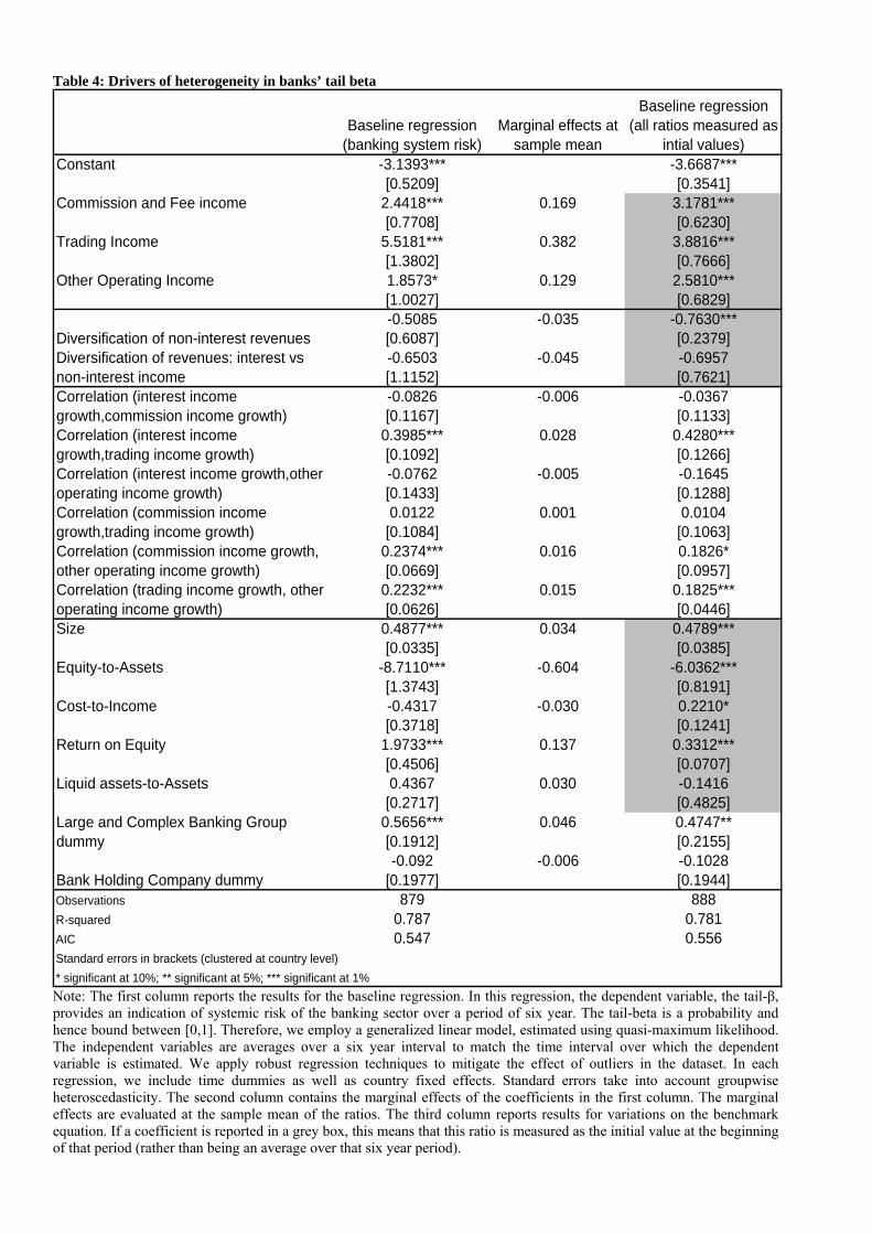
The results14 shown in column 1 of Table 4 re�ect the relationships between various bank-speci�c variables

and banks' tail beta measure. The tail beta measures the probability of observing a correction in a bank's

equity return conditional on observing a large drop in the European Union banking sector index. From Table

4, it can be seen that interest income is less risky than all other revenue streams. This can be inferred from

the observation that the coef�cients of all other revenue shares are positive. This means that the alternative

revenue streams have a bigger impact on banks' extreme risk measures than those originating from traditional

intermediation activities. Put differently, the tail beta of a diversi�ed bank is higher than the tail beta of a bank

specialized in interest-generating activities. The coef�cient on the share of trading income is the largest of

the non-traditional revenue sources and its impact differs signi�cantly from the other shares. The estimation

results reveal that other indicators of bank specialization in traditional intermediation corroborate the �nding

that traditional banking activities result in lower systemic risk. Hence, we can conclude that banks that focus13More information on how to obtain the set of LCBGs can be found in a special feature article of the ECB Financial Stability Review

of December 2006. Based on a multiple indicator approach, i.e. cluster analysis, 33 banking groups are identi�ed as LCBGs. 24 of these

are located in the EU15, but not all of them are listed.14The baseline results are obtained for a restricted sample of commercial banks and bank holding companies. We impose two restrictions

on the sample used in the baseline. First, we eliminated non-diversi�ed/specialized banks from the sample. That is, we only include banks

with an interest income share between 10% and 90%. Furthermore, we also eliminate fast-growing banks. For these banks, the correlation

between each pair of growth rates of the different revenue types may be biased and overstate the true degree of revenue correlation. In the

robustness section, we document that these restrictions have little impact on the baseline results.

22

on lending activities are less exposed to systemic banking risk than diversi�ed banks15.


The diversi�cation measures do not enter the equation signi�cantly. Apparently, having a more equally-

balanced portfolio of revenue streams (either between interest and non-interest income or within non-interest

income revenue) seems not to reduce or increase a bank's tail beta. On the other hand, the extent to which

the growth rates of the various revenue streams are correlated does play an important role. The signi�cant

coef�cients are positive, as portfolio theory predicts. Imperfectly correlated revenue streams should reduce

bank risk. A low correlation between shocks to interest income and trading income reduces banks' tail-�

signi�cantly. Furthermore, a low correlation between shocks of any of the non-interest income types also

contributes positively to overall banking system stability. These results imply that even though banks may have

equal revenue shares, their risk pro�le may be substantially different depending on the correlation16 between

the revenue types.

The other bank-speci�c variables also reveal interesting relationships. Size is by far the most signi�cant

driver of banks' tail betas. Recall that the conditioning event is a crash in the European banking index, ex-

cluding the bank for which we compute the tail beta to avoid spurious results. Larger banks are inherently

more exposed to many sectors in many countries and are hence more tied to European-wide shocks. Large

drops in small banks' stock price are more likely to be idiosyncratic events or are more tied to local factors

since small banks are predominantly active in their home country. In addition to the size effect, the dummy

for Large and Complex Banking Groups is also associated with higher tail betas. In recent years, mergers,

acquisitions and organic growth have meant that some of the largest and most complex �nancial groups have

come to transcend national boundaries and traditionally de�ned businesslines. As a result, they have become

a potential channel for the cross-border and cross-market transmission of �nancial shocks (Hawkesby, Marsh15This conclusion is con�rmed when including measures of market power and specialization in traditional banking markets in the

regression. Banks with a higher interest margin or a higher loans-to-asset ratio are perceived to contribute less to banking system instability

since higher values of these ratios reduce banks' tail betas. However, these variables are strongly correlated with the revenue shares, which

affect both the magnitude and the precision of the estimated coef�cients. Therefore we do not include them in the baseline speci�cation.16The correlations might be considered as generated regressors. Consequently, it is important to check whether the other coef�cients

and their standard errors are affected by including them. We also do the entire analysis without the correlation measures and observe that

the coef�cients and the standard errors of the other variables are remarkably unaltered.

23

and Stevens, 2007). Apparently, the banks at the heart of the �nancial system, which need to be monitored

closely, contribute negatively to banking system stability. To check that the main results of the paper are not

just a result of comparing small and large banks, we report in the robustness section results for various equally

large subsamples (based on bank size). The capital-to-asset ratio exhibits the expected sign and is signi�cant.

A larger capital buffer increases a bank's contribution to banking system stability. Ef�ciency and liquidity do

not enter the equation signi�cantly. Banks that generate high pro�ts ('in excess of their fundamentals') are

much riskier. This mirrors the common risk-return trade-off. The causality in this relationship may, however,

run in the other direction. Banks may gamble and increase their exposure to risky activities that may yield

higher pro�ts. A similar critique may hold for other relationships as well.

Next to return on equity, the equity-to-asset ratio may also suffer from reverse causality if banks' capital

buffers are eroded from unexpected losses due to the more riskier income activity. Some of the relationships

may be plagued by endogeneity. That is, the relationships could occur if riskier banks engage in non-traditional

banking activities, rather than the reverse. Finally, given that the risk measure is based on stock market values,

there might be a spurious relationship between trading income and tail betas. These possibilities can be checked

by looking at the initial values of the ratio at the beginning of that six-year period rather than the average values

over the six years. In Column 3 of Table 4, all accounting variables are measured as initial values. Some in-

teresting conclusions can be drawn from this analysis. First, trading income is still signi�cant, which indicates

that trading income causally affects bank risk. The other alternative revenue shares also remain signi�cant.

Second, return on equity has a lower impact. This indicates that part of the risk-return relationship is due to

the higher pro�ts that risky activities generate. The bank's average pro�ts over that period will be higher if

a bank takes on more risk (as measured over a six year period). Nevertheless, the initial pro�tability level is

also signi�cantly and positively related to a bank's tail beta. Finally, a bank's initial capital ratio signi�cantly

reduces its exposure to systemic banking risk. The tail betas of banks that are �nancially strong banks at the

beginning of the period are less affected by a crash in the EU banking sector index. In the last subsection, we

document that these results are robust to potential reverse causality or endogeneity created by events such as

mergers and acquisitions, delistings, or systemic crises.

Analyzing the economic impact of revenue diversi�cation on banking system stability

24

Until now, we focussed the description of the results on the interpretation of the sign and the signi�cance.

To assess the magnitude of the coef�cients and their economic impact we have to rely on �tted marginal ef-

fects. Both the (logistic) link function and the level of the variables affect the estimated effect of a change in

one variable on the tail-�. That is:

@E [TAIL� jX� ]@Xi

=@g(X�)

@Xi= b�i exp(Xb�)�

1 + exp(Xb�)�2 (9)

In column 2 of Table 4, we report the marginal effects of each variable when the expression in Equation

(9) is evaluated at the sample means. The marginal effects of the three non-interest revenue shares vary in the

range of 0:13 to 0:38. The effect is largest if a bank reallocates revenues from Interest activities to Trading

Income activities. To get more insight in this number, consider the following event. Over the sample period,

the average share of net interest income in total income decreased by more than 12%. All else equal, this shift

of 12% of total revenues from the interest activities to non-traditional banking activities yields an increase in

the average bank's tail-� in the range of 1:5 � 4:6 basis points. If an expansion into non-traditional banking

is accompanied by a reduction in a bank's outstanding loans and interest margin, this may further increase the

tail-�. Depending on the time period, an increase with 3:0 basis points corresponds to 30% of the median tail-�

in 1994-1999 and almost 100% in 1999-2004.

A bank that keeps its revenue shares unchanged, but would be faced with less correlated interest income

and trading income, will observe a drop in its tail-�. If this correlation drops from the sample mean (0:178) to

that of the 5th percentile (�:767), the tail beta will be almost 2:6 basis points lower. Hence, both the type of

income and their correlation play an important role in increasing banking system stability.

Controlling for non-traditional banking activities, we discover that a larger capital buffer in �nancial institu-

tions will exert a mitigating effect on systemic risk. An increase of the equity-to-assets ratio of 0:05 will result,

all else equal, in a drop in the tail beta of 3 basis points. Bank size is by far the most important contributor to

heterogeneity in tail risk. Consider two banks that only differ in size, one bank has the average size while the

value of the total assets of the other bank is �xed at the 75th percentile. The difference in tail-� exceeds 0:05.

The larger bank will have, all else equal, a 5% higher probability of a large drop in its stock return if there is

a large, negative shock to the European banking sector index. This increase equals a substantial proportion of25

the average tail-�. Depending on the time period, an increase with �ve basis points corresponds to 30% of the

average tail-� in 1994-1999 and 50% of the average tail-� in 1999-2004. In addition, LCBGs have a tail beta

that is, all else equal, 4:6 basis points higher.

The marginal effects are not constant; they depend on the values at which X is evaluated. Hence, although

the argument within the link function is a parsimonious linear model, we are able to capture both non-linear

relationships and interaction effects. On the one hand we can compute the marginal effect of a change in the

variableXi for different values ofXi while �xing the values of the other variables (at e.g. their sample mean).

We learn that the implied effects differ substantially when they are assessed at other values than the mean.

The marginal effect of a change in one of the revenue shares increases monotonously with the value of that

variable. But the slope differs across the revenue shares. The impact of other operating income only increases

moderately, largely due to the smaller range over which this revenue share is observed. The marginal effect of

an increase in the trading income share on banks' tail beta is 0:38 at the sample mean (which is 6% of total

income). The impact is around 0:30, if an otherwise equal bank only derives a small proportion (1%) of its

income from trading activities. On the other hand, a bank with an even greater reliance on trading income, 16%

of total operating income, will have a marginal effect of 0:60, which is two times larger than the bank in the

latter case.

On the other hand, we are also able to assess the impact of a change in Xi for banks that only differ

with respect to another variable Xj . Consider again the benchmark values of the average bank (as reported in

column 2 of Table 4). At the mean trading income share, the marginal effect is 0:38. Since a larger capital buffer

reduces banks' tail beta, the impact will be larger for less capitalized banks. The differential impact between

the low and high capital ratio banks is 0:09 at the sample mean of trading income. This impact gap widens

for banks that are more heavily involved in trading income generating activities and is for instance 0:13 when

the trading income share is 16%. Put differently, in order to experience similar marginal effects of an increase

in trading income, a better capitalized bank may already be more involved in this riskier revenue source. This

con�rms the presence of an interaction effect between the degree of capitalization and a bank's involvement in

non-interest generating activities. Consequently, one could argue that regulatory capital requirements should

be related to banks' reliance on trading income. Similarly, bank size is an important contributor in explaining

differences in heterogeneity in bank tail risk. The marginal impact differs substantially for large and small

26

banks. The interaction effects are even more apparent, especially for commission and trading income. The gap

in marginal impacts of an increase in non-interest generating activities (in small versus large banks) widens

substantially for larger shares of the associated revenue type.

5.2 Tail dependence versus central dependence

We are interested in assessing the extent to which individual banks are exposed to a severe aggregate shock, as

captured by an extreme downturn in the EU banking sector index. For that purpose, multivariate extreme value

analysis is a well-suited technique since it accounts for the fat tails that are inherent to stock prices and it is

not tied to speci�c distributional assumptions. In general, most authors focus on risk during normal conditions.

Dependency in the center of the distribution is typically measured using a �rm's beta or a correlation coef�cient,

which both describe the sensitivity of an asset's returns to broad market or (bank) sector movements. While

measures of dependence in the tails and the center are theoretically distinct concepts, they may share several

features. For reasons of comparability with the tail-�, we measure banks' normal risk exposures to the banking

index over moving windows of six years. The �rst period covers the years 1992-1997. In each subsequent

subsample, we drop the observations of the initial sample year and add a more recent year of data. We analyze

the information content of the dependence concepts and arrive at a number of interesting conclusions.

First, the rank correlation between the tail beta and the ordinary beta is very high. Across the eleven

time windows of six years, it �uctuates in the range of 50% to 75%. Hence, banks with a large exposure to

movements in the banking index in normal economic conditions will be more exposed to extreme movements as

well. The high correlation implies that both dependence measures share an important component. Second, we

establish signi�cant relationships between non-traditional banking activities and systemic bank risk exposures

(see Column 1 of Table 4 and 5). We run similar regressions, but substitute the dependent variable. The results

are reported in Columns 2 of Table 5.


The tail beta is replaced as dependent variable by the OLS beta (obtained by regressing bank returns on

returns on an EU banking index). We discover similar relationships. All non-interest generating activities

increase the exposure of banks' stock returns to movements in the EU banking index. The impact of trading

income is signi�cantly larger than the impact of commission income and other operating income. Contrary27

to expectations, banks' OLS beta will be higher the more equal are the shares of interest and non-interest

income. The coef�cient on HHIREV is negative and signi�cant. The six measures of the correlation between

shocks to pairs of income shares are all positively related to the OLS beta of a bank's stock return. Five

of them are statistically signi�cant. The largest potential for risk reduction can be obtained by combining

imperfectly correlated interest and commission income generating activities. Furthermore, larger banks and

less-capitalized banks have higher betas. In light of the previous �nding, the high correlation between central

and tail dependence measures, these observations are far from surprising. The more interesting issue is whether

bank characteristics, and especially bank's income structure, can explain the residual heterogeneity in the tail-�

that is not explained by central dependence measures.

Therefore, we add the OLS beta to the baseline regression (Column 3 of Table 5). Doing so, we want to

decompose the effect of bank-speci�c variables on the tail betas into a direct effect and an indirect effect. The

direct effects are the estimated relationships between a variable and the tail-beta. The indirect effect captures

how a variable affects risk both in normal and extreme conditions and runs through the impact of the central

dependence measure. Due to the large positive correlation, we expect and �nd a highly signi�cant relationship

between the traditional dependence measure and the tail beta. Hence, an increase in, for instance, the share of

commission or trading income will indirectly result in an increase of the tail beta. If any of the bank-speci�c

variables exhibit a signi�cant17 relationship with the tail beta, this implies that there is a direct effect that

increases extreme bank risk in addition to the indirect effect.

When the central dependence measures are taken into account, we obtain that all non-traditional banking

activities contribute positively to systemic banking risk. However, only the share of trading income in total in-

come is signi�cant at the conventional signi�cance levels. Furthermore, a stronger correlation between shocks

to other operating income and both other non-interest income sources, as well as between interest income and

trading income, increases banks' tail-�. Measures of bank size and bank pro�tability are signi�cant and hence

enforce the positive indirect effect. Fourth, in column 4 Table 5, we report a joint effect18, which is the sum of

the direct (coef�cients in Column 3) and indirect effect (coef�cient on the central dependence measure times17From Column 2 of Table 5, we learn that many bank-speci�c variables have a large partial correlation coef�cient with the central

dependence measure. This may create a multicollinearity problem and hence harms �nding signi�cant relationships by in�ating the

standard errors in Column 3 of Table 5. Therefore, we focus more on the magnitude of the coef�cient rather than the signi�cance level.18The joint effects are, as expected, similar in magnitude to the coef�cients reported in Column 1.

28

the estimated coef�cients in Column 2). It is interesting to compare the direct effects, the coef�cients in Col-

umn 3, with the joint effects in Column 4. For instance, the direct effect of an increase in commission income,

trading income, or other operating income on a bank's extreme risk pro�le is larger than the indirect effect.

The impact of correlated shocks also works predominantly via the direct effect. Reassuring for bank capital

regulation is that the stabilizing impact of large capital buffers is stronger in turbulent times than in normal

economic conditions.

To conclude, we discover a high correlation between banks' systemic risk exposures in normal and stress

periods. Furthermore, the shift to non-traditional banking activities has increased banks' OLS beta and as a

consequence their tail beta. However, there is also an additional and, for most variables, an even larger direct

effect on banks' tail betas. The information content of tail betas differs from measures focussing on central

dependence. In the robustness section, we also show that the information content of tail betas differs from other

composite risk measures such as long-term debt ratings or equity return volatility.

5.3 Support for the baseline equation

Many banks are not included in all subperiods. Hence, the panel data set is unbalanced. If selection in the

sample occurs randomly, then the results of the baseline regression are not subject to bias. However, some

sources of sample selection are potentially non-random and may affect the estimated relationships. First, bank

stocks that are traded infrequently are excluded since the risk measure will not be informative. Furthermore,

some banks either entered the sample after an IPO or dropped out due to a delisting. These three events

have in common that accounting data are available for the entire period but stock price information is not

available or useful for the entire period 1992-2007. Another important source of unbalancedness are mergers

and acquisitions. We examine the aforementioned selection issues simultaneously19. The estimation results

are documented in Table 6. Column 1 contains the results for a substantially reduced sample. The sample19We can also estimate a Heckman (1976) selection model for these events. Given that we consider multiple selection events, we

implement a two-step procedure. Initially, we estimate three different selection equations (probit regressions). The dummy is one if

that bank-time observation is included in the �nal sample and zero otherwise. Subsequently, we compute the Inverse Mills ratio (or

selection hazard) for each selection equation and incorporate them in the baseline equation. We obtain that none of the Inverse Mills

ratios is signi�cant at the traditional signi�cance levels. Accounting for non-randomness in the sample selection alters the marginal effects

(slightly) but not the signi�cance.

29

size reduces to 530 observations as a result of dropping banks that are involved in one or more of the selection

criteria. In column 2, we report results for the initial sample size but include (not reported) dummy variables for

the various potential sample selection problems. The results do not change qualitatively, an exception being the

loss of signi�cance of the other operating income share. However, in the smaller sample almost all coef�cients

are larger in absolute value. Regarding the dummy variables, we observe that banks whose shares are traded

infrequently have lower tail betas. These banks are typically smaller banks, which strengthens the �ndings

on bank size. To conclude, although the panel dataset is unbalanced, the sources of the missing values in the

dataset do not affect the relationships of interest.


Some European countries confronted a banking crisis20 in the beginning of the nineties. Especially for the

Scandinavian countries, the crises in the banking industry were severe in terms of output loss as a percentage

of GDP. Given the focus on heterogeneity in banks' extreme risk pro�les, these unusual events may drive the

results. In column 3 of Table 6, we exclude a bank-time observation if this bank has been active in a country

that experienced a banking crisis during one of the six years of that time frame. The results reported in Column

6 show that including the crisis periods does not affect the results (again, except for the share of other operating

income in total income). The coef�cients on the alternative revenue shares and the correlation coef�cients are

of a similar magnitude as those reported in Table 4, which further strengthens the stability of our �ndings.

The independent variables proxy strategic choices made by banks and capture information on capital, man-

agement, earnings and liquidity. Similar information might be contained in aggregated proxies of bank behav-

ior, such as ratings or market-based information. In fact, the results in Table 5 document that there is indeed a

relationship between bank's beta in normal and stress times, but that many independent variables have an addi-

tional impact. In columns 4-6, we include a rating on long-term bank debt, a measure of idiosyncratic volatility

of banks' equity returns, and total volatility of bank equity returns. Concerning column 4 of Table 6, we follow

Pop (2006) and construct the mean of long-term issuer ratings assigned by S&P, Moody's and Fitch. Before20Information on the timing and magnitude of the crisis is obtained from the Worldbank Database of Banking Crises (Caprio, 2003).

Six countries experienced a banking crisis during the sample period: Denmark (1992), Finland (1992-1994), France (1994-1995), Greece

(1992-1995), Italy (1992-1995) and Sweden (1992-1995). Note that we only report the years that occur in the sample period, some crises

started earlier.

30

averaging, the ratings are �rst converted to cardinal values using Pop's scale. The lower the cardinal value, the

more creditworthy is the issuer. Including this rating reduces the sample size considerably to 360 observations.

The coef�cient on the long-term rating is measured imprecisely and is hence insigni�cant. More important,

the results regarding the other coef�cients are almost unaltered. Changes with respect to the baseline are the

following: the coef�cient on the other operating income share reduces considerably. Return on equity is only

marginally signi�cant, but this is due to the larger standard error because of the smaller sample rather than a

change in the coef�cient. All other coef�cients are of equal size compared to the baseline regression without

the rating, but the standard errors are larger. From column 5 and 6 of Table 6, we can infer that aggregate

market-based measures of bank risk are not related to the tail beta. The results in both columns are almost ex-

actly equal. The coef�cient on the liquid assets to total assets ratio is slightly higher in the regression with total

volatility. This, combined with a smaller standard error, yields a signi�cant and positive relationship between

this ratio and the tail beta. Apparently, additional measures of bank risk (total volatility, idiosyncratic volatility,

rating on long term debt) do not enter the equation signi�cantly nor do they affect the estimated coef�cients on

the other variables. This further underlines the fact that the information content of tail betas is different from

other proxies of risk.

One of the most signi�cant variables in determining tail betas is bank size. To check that the main results of

the paper are not just a result of comparing small and large banks, we redo the analysis for various subsamples.

We rank the banks according to size and split the sample in three equally large subsamples. The mean bank

size of the smallest third is 7; 989 million euro. The average bank in the middle group has 54; 025 million

euro of total assets. Average total assets in the group of large banks equals 241; 680 million euro. Performing

the analysis on the three different subsamples does indeed yield further insights. We present the results in

columns 1-3 of Table 7. First, many of the obtained results hold for each subsample. Larger banks, less

capitalized banks, LCBGs and banks with a large share of trading income have higher tail betas. Second, the

impact of commission income and other operating income on tail betas is signi�cant for the subsets of small

and medium-sized banks, but not for the subsample of the largest banks. For the largest banks, only trading

income is perceived as a more risky revenue stream. Third, the impact of the correlation between pairs of

revenue streams is largely similar across the three different subsamples. Fourth, the effect of cost-to-income

and diversi�cation (HHI-revenue) on tail betas differs substantially in the three subsamples. That is, we observe

31

signi�cant relationships with opposite signs, which is probably causing the insigni�cance of these variables in

the overall sample. From this we can conclude that the baseline results are not merely a result of comparing

small and large banks. Nevertheless, looking at various subsamples of banks with different size yields further

insights into the determinants of systemic banking risk.


The baseline results are obtained for a sample of commercial banks and bank holding companies. However,

since the purpose of this research is to investigate the impact of diversi�cation strategies on banking stability, we

further imposed two restrictions on the sample used in the baseline. First, we eliminated non-diversi�ed banks

from the sample. That is, we only include banks with an interest income share between 10% and 90%. Banks

not satisfying this criterion are categorized as too specialized. Furthermore, we also eliminate fast-growing

banks. For these banks, the correlation between each pair of growth rates of the different revenue types may be

biased and overstate the true degree of revenue correlation. Column 4 of Table 7 reports the results when we

drop these restrictions and hence employ the full sample of commercial banks and bank holding companies. In

this case, the sample size increases by 10% to 980 observations. All results established in Table 4 still hold.

However, in the full sample the magnitude of the impact of the equity-to-asset ratio is substantially reduced (but

still signi�cant). In addition, we obtain that the Her�ndahl Hirschmann index of the non-interest generating

activities is negatively and signi�cantly related to banks' tail-�. This unexpected result indicates that banks'

risk pro�le will be improved if they focus their non-interest income. However, this is predominantly caused

by a few banks that derive more than 90% of their income from non-traditional banking activities and should

therefore be considered as outliers in a sample of commercial banks and BHCs.

Finally, we perform two robustness checks in which we zoom in on the dependent variable. First, we ac-

knowledge that the dependent variable is an estimated variable and may hence be subject to measurement error.

Variation in the sampling variance of the observations on the dependent variable will induce heteroscedastic-

ity. Given the two-step procedure, we obtain information on part of this heteroscedasticity. We implement

Hanushek's FGLS method (1974), which takes into account both the variance of the homoscedastic noise and

the heteroscedasticity of the sampling errors. Note, however, that we now are no longer able to implement

the weighting schemes we apply in the baseline regression to obtain robust regression results. We report the

results in column 5 of Table 7. As in most robustness checks, the results are largely unaffected. Differences in32

signi�cance with respect to the baseline (�rst column of Table 4) are only observed for two variables. The co-

ef�cients on other operating income and the correlation between shocks to trading and other operating income

are signi�cant in the baseline but not in this robustness check (though the estimates don't differ signi�cantly

from one another). We prefer robust regression methods over Hanushek FGLS method as the baseline, since the

R-squared is much higher in the former compared to using FGLS. This provides an indication that controlling

for outliers and robust standard errors is more important than taking into account the uncertainty introduced by

the estimated dependent variable. Second, the paper deals with systemic banking risk and measures tail betas

with respect to a European banking index. However, one could easily measure the tail beta of bank stock returns

with respect to a general European market index. This measure would provide an indication of extreme system-

atic risk exposures. In the last column of Table 7, we replace our proxy of systemic risk with one of extreme

systematic risk. That is, the dependent variable now captures the probability that a bank's equity return crashes,

conditional on observing a market-wide correction. The results are very similar, which need not be surprising.

First, given banks' central role in the economy, corrections in a banking sector index will most likely occur

on days of broad market corrections and vice versa. Second, a large part of banks' commission and trading

income stems from structured �nance activities. A largely neglected feature of the securitization process is that

it substitutes risks that are largely diversi�able for risks that are highly linked to events in the economy. Coval

et al. (2009) document that the senior tranches of structured �nance products have signi�cantly higher system-

atic risk exposures, especially with respect to credit rating-matched, single-name counterparts. Consequently,

these senior structured �nance claims have the features of economic catastrophe bonds, as they are designed to

default only in the event of extreme economic distress (Coval et al., 2008). A third explanation is offered by

Pennacchi (2006), who models a bank's choice of investments when deposit insurance and capital standards are

risk-based. His model predicts that banks would choose to sell credit protection for loans and bonds of �rms

with a high systematic risk of default. Moreover, deposit insurance provides a bank with incentives to engage

more in the fee-generating business of providing loan commitments. However, the latter are the least pro�table

in the bad states of the world when �rms' credit quality turns out to be low.

Both Coval et al. (2009) and Pennacchi (2006) argue that the existing capital requirements may have

subsidized systematic risks. The existing requirements depend on credit risk assessments, either internal or

by rating agencies, that focus on the probability of default and the loss given default. An important aspect of

33

credit risk that is neglected by rating agencies and regulators is the timing of the default or the conditions in

which default is likely to happen. Kupiec (2004) remarks that all of the New Basel Accord's proposed capital

schemes contain incentives that may encourage banks to purposely concentrate on credits that are expected to

default in recessions. Morever, banks may also be inclined to select the timing of default to enhance the value

of their deposit insurance guarantee (Kupiec, 2004). Hence, as long as capital regulation or deposit insurance

premiums fail to include a premium for systematic risk, banks will have an incentive to take extreme systematic

risks, by engaging in non-interest activities.

6 Conclusion

The banking sector occupies a central role in every economy and is a particularly important sector for the

stability of �nancial systems. As a result, central bankers and �nancial supervisors invest a great deal of re-

sources in analyzing how to strengthen the �nancial system, including the system of �nancial regulation and

supervision, to reduce the frequency and severity of future bouts of �nancial instability. Reliable indicators of

banking system stability are of the utmost importance. In this paper, we employ a recent approach to assess

banking system risk (Hartmann et al., 2006). This statistical approach assesses the joint occurrence of very rare

events, such as severe banking problems. More speci�cally, the bank-speci�c systemic risk measure captures

the probability of a sharp decline in a bank's stock price conditional on a crash in a European banking sector

index. We discover considerable heterogeneity in banks' contributions to overall banking sector stability. This

observation should not be surprising in light of some remarkable developments over the last decades. Sub-

stantial banking consolidation, the dismantling of the legal barriers to the integration of �nancial services, and

technological evolution all affected the organizational design of banking �rms. These developments initiated

the emergence of large and complex banking organizations. Yet some banks continue to specialize in traditional

intermediation activities or target local customers.

When relating the tail betas to bank-speci�c accounting variables, we can explain a fair amount of the

cross-sectional dispersion in extreme bank risk. We establish that the shift to non-traditional banking activities

increases banks' tail betas and thus reduces banking system stability because interest income is less risky

than all other revenue streams. Moreover, the impact of the alternative revenue shares (commission and fee

income, trading income, other operating income) do differ substantially from one another. Other indicators of34

bank specialization in traditional intermediation, such as the net interest margin and the loans-to-assets ratio,

corroborate the �nding that traditional banking activities are less risky. Hence, we can conclude that banks

that pro�tably focus on lending activities contribute more to banking system stability than diversi�ed banks.

This questions the usefulness of �nancial conglomeration as a risk diversi�cation device, at least in times of

stock market turmoil. Retail banks, with a relatively high proportion of core deposits and loans in total assets,

have a consistently lower systemic risk exposure. Moreover, as long as capital regulation or deposit insurance

premiums fail to include a premium for systematic risk, banks will have an incentive to take extreme systematic

risks by engaging in non-interest activities.

The established relationships bear implications for bank supervision. Bank size is by far the most signi�cant

driver of banks' tail betas. Some particularly thorny issues are raised by the existence of �nancial institutions

that may be perceived as "too big to fail" and the moral hazard issues that may arise when governments in-

tervene in a �nancial crisis. The latter could be perceived as an implicit expansion of the safety net and may

exacerbate the problem of "too big to fail," possibly resulting in excessive risk-taking and still greater systemic

risk in the future. Moreover, since the large banks are more exposed to European-wide (banking) shocks and

economic conditions, their prudential supervision needs to take that feature into account. In Europe, increas-

ing banking sector integration initiated by directives that led to the single market for �nancial services further

complicated the tasks of national and supranational supervisors. This will be even more the case when banks

further increase their cross-border activities, which strengthens the need for an integrated European supervisor

for internationally operating banks. For the locally operating banks, supervision at the country level should

suf�ce to assess the implications of their risk pro�le.

In addition, the results are interesting in light of the third pillar of Basel II. Market participants, in addition to

armies of regulators, will do some of the work in assessing the overall risk position of the bank. A larger capital

buffer decreases a bank's exposure to extreme shocks. This �nding is expected and underlines the importance of

capital adequacy as a signal of bank creditworthiness. Furthermore, a more complete and coherent disclosure of

the different revenue streams facilitates a better understanding of the risks being taken by different institutions.

The debate on the optimality and desirability of universal banking and �nancial conglomerates is still unsettled.

Some blame the recent banking crisis of 2008 on a lack of regulation of certain �nancial activities or even

deregulation with respect to the combination of commercial and investment banking. While it is unknown to

35

what extent the crisis could have been avoided by more regulation, more disclosure and transparency of the

different �nancial activities and the associated revenue streams would have helped in mitigating, identifying,

and resolving many problems. Therefore, in European banking, steps need to be taken in order to get a more

detailed and consistent picture of the underlying components of non-interest revenue, especially with respect

to commission and fee income. The US reporting requirements, which since March 2001 include a 12-item

distinction of non-interest income, may be a useful benchmark.

36

References

[1] Acharya, V. (2009). "A Theory of Systemic Risk and Design of Prudential Bank Regulation." Journal of

Financial Stability, article in press.

[2] Arellano, M. (2003) "Panel data econometrics (Advanced texts in econometrics)." Oxford University

Press, p. 244.

[3] Baele, L., O. De Jonghe, and R. Vander Vennet (2007). "Does the stock market value bank diversi�ca-

tion?" J. Banking Finance 31, 1999-2023.

[4] Barth, J., G. Caprio and R. Levine. (2004). "Bank Regulation and Supervision: What Works Best?" J.

Finan. Intermediation 13, 205-248.

[5] Beck, T., A. Demirguc-Kunt and R. Levine. (2006). "Bank Concentration, Competition, and Crises: First

Results." J. Banking Finance 30, 1581-1603.

[6] Berk, R. A. (1990). "A primer on robust regression.", in Modern Methods of Data Analysis, eds. J. Fox

and J. S. Long, Saga Publications, 292-324.

[7] Caprio, G. (2003). "Episodes of systemic and borderline �nancial crises." Worldbank Database of Bank-

ing Crises.

[8] Cihák, M. and K. Schaeck (2007). �How Well Do Aggregate Bank Ratios Identify Banking Problems?"

IMF Working Papers, 1-40.

[9] Coval, J.D., J.W. Jurek, and E. Stafford. (2008) "Economic Catastrophe Bonds." Amer. Econ. Rev. ,

forthcoming.

[10] Coval, J.D., J.W. Jurek, and E. Stafford. (2009). "The Economics of Structured Finance." J. Econ. Per-

spect. 23, 3-25.

[11] Danielsson, J., L. de Haan, L. Peng and C. G. de Vries. (2001). "Using a bootstrap method to choose the

sample fraction in tail index estimation." Journal of Multivariate Analysis 76, 226-248.37

[12] de Bandt, O. And P. Hartmann. (2002). "Systemic risks in Banking." in Financial crisis, contagion and

the Lender of Last resort, edited by C. Goodhart and G. Illing, Oxford University Press.

[13] de Haan, L., D.W. Jansen, K. Koedijk, and C.G. de Vries. (1994). "Safety �rst portfolio selection, extreme

value theory and long run asset risks." in J. Galambos, J. Lechner and E. Simiu (eds.), Extreme Value

Theory and Applications (Dordrecht: Kluwer Academic Publishers), 471-487.

[14] Demirgüc-Kunt, A. and E. Detragiache. (1998). "The determinants of banking crises in developing and

developed countries." Int. Monet. Fund Staff Papers 45, 81-109.

[15] Demirgüc-Kunt, A. and E. Detragiache. (2002). "Does deposit insurance increase banking system stabil-

ity? An empirical investigation." J. Monet. Econ. 49, 1373-1406.

[16] Deng, S., E. Elyasiani, and C. Mao. (2007). "Diversi�cation and the cost of debt of bank holding compa-

nies." J. Banking Finance 31, 2453�2473.

[17] de Nicolo, G., P. Barthlomew, J. Zaman, and M. Zephirin. (2004). "Bank consolidation, internationaliza-

tion, and conglomeration: trends and implications for �nancial risk." Finan. Markets, Inst. Instruments

13, p. 173-217

[18] DeYoung, R. and K.P. Roland. (2001). "Product mix and earnings volatility at commercial banks: Evi-

dence from a degree of total leverage model." J. Finan. Intermediation 10, 54-84.

[19] Dewatripont, M., and J. Mitchell. (2005). "Risk-taking in �nancial conglomerates." Work in progress.

[20] Draisma G., H. Drees, A. Ferreira and L. De Haan. (2004). "Bivariate tail estimation: dependence in

asymptotic independence." Bernoulli 10, 251-280.

[21] Eichengreen, B. and A. Rose.(1998). "Staying A�oat When the Wind Shifts: External Factors and

Emerging-Market Banking Crises.", National Bureau of Economic Research Working Paper 6370.

[22] Embrechts P., C. Klüppelberg, C., and T. Mikosch. (1997). "Modelling extremal events for insurance and

�nance." Springer: Berlin.

[23] Fama, E., and J. MacBeth. (1973). "Risk, return and equilibrium: Empirical tests." J. Polit. Economy 81,

607-636.38

[24] Freixas, X., G. Loranth and A. Morrison. (2007). "Regulating �nancial conglomerates." J. Finan. Inter-

mediation 16, 479-514.

[25] Gorton, G. (1988). "Banking panics and business cycles. " Oxford Econ. Pap. 40, 751-781.

[26] Gropp, R., J. Vesala, and G. Vulpes. (2006). "Equity and bond market signals as leading indicators of

bank fragility." J. Money, Credit, Banking 38, 399-428.

[27] Hanushek, E.A. (1974). "Ef�cient estimators for regressing regression coef�cients". Amer. Statistician

28, 66�67.

[28] Hartmann, P., S. Straetmans and C. G. de Vries (2006). "Banking system stability: a cross-atlantic per-

spective." in The Risks of Financial Institutions, eds. Mark Carey and Rene Stulz; National Bureau of

Economic Research Conference Report.

[29] Hawkesby, C., I. Marsh and I. Stevens. (2007). "Comovements in the equity prices of large complex

�nancial institutions." Journal of Financial Stability 2, 391-411.

[30] Heckman, J.J. (1976). "The common structure of statistical models of truncation, sample selection, and

limited dependent variable models and a simple estimator for such models." Ann. Econ. Soc. Meas. 5,

475-492.

[31] Hill, B. M. (1975). "A simple general approach to inference about the tail of a distribution." The Annals

of Statistics, 3, 1163-1173.

[32] Houston, J., C. Lin, P. Lin and Y Ma. (2008). "Creditor rights, information sharing, and bank risk taking."

Unpublished manuscript, http://ssrn.com/abstract=1318458.

[33] Huber, P.J. (1981). "Robust statistics." New York, John Wiley and Sons.

[34] Huisman, R., K.G. Koedijk, C.J.M. Kool, and F. Palm. (2001). "Tail-index estimates in small samples." J.

Bus. Econ. Statist. 19:1, 208-216.

[35] Kaminsky, G.L. and C.M. Reinhart. (1999). "The twin crises: The causes of banking and balance-of-

payments problems." Amer. Econ. Rev. 89, 473-500.

39

[36] Kieschnick, R., and B.D. McCullough (2003). "Regression analysis of variates observed on (0, 1): per-

centages, proportions and fractions." Statistical Modelling 3, 193-213.

[37] Kupiec, P. (2004). "Is the New Basel Accord Incentive Compatible?" in Benton Gup (Ed.), The New Basel

Capital Accord, Thompson South-Western Publishers.

[38] Kwan, S.H., and E. S. Laderman. (1999). "On the portfolio effects of �nancial convergence: A review of

the literature." Fed. Reserve Bank San Francisco Rev. 2, 18-31.

[39] Laeven, L. and R. Levine. (2007). "Is there a diversi�cation discount in �nancial conglomerates?" J.

Finan. Econ. 85, 331-367.

[40] Ledford, A., Tawn J. (1996). "Statistics for near independence in multivariate extreme values." Biometrika

83, 169-187.

[41] Lepetit, L., E. Nys, P. Rous and A. Tarazi (2008). Bank income structure and risk: An empirical analysis

of European banks." J. Banking Finance 32, 1452-1467 .

[42] Mercieca, S., K. Schaeck and S. Wolfe (2007). "Small European banks: Bene�ts from diversi�cation?" J.

Banking Finance 31, 1975-1998.

[43] Papke, L.E., and J.M. Wooldridge (1996). "Econometric methods for fractional response variables with

an application to 401 (K) Plan participation rates." J. Appl. Econometrics 11, 619-632.

[44] Pastor, L., and P. Veronesi. (2005). "Rational IPO waves." J. Finance 60, 1713�1757.

[45] Pennacchi, G. (2006), "Deposit Insurance, Bank Regulation, and Financial System Risks." J. Monet.

Econ. 53, 1-30.

[46] Petersen, M. (2009). "Estimating standard errors in �nance panel data sets: Comparing approaches." Rev.

Finan. Stud. 22, 435-480.

[47] Poon, S.-H., M. Rockinger and J. Tawn. (2004). "Extreme value dependence in �nancial markets: Diag-

nostics, models and �nancial implications." Rev. Finan. Stud. 17, 581-610.

[48] Pop, A. (2006). "Market discipline in international banking regulation: keeping the playing �eld level."

Journal of Financial Stability 2, 286-310.40

[49] Rajan, R.G. (2006). "Has �nancial development made the world riskier? Europ. Finan. Manage. 12, 499-

533.

[50] Santos, J. (2001). "Bank Capital Regulation in Contemporary Banking Theory: A Review of the Litera-

ture." Finan. Markets, Inst. Instruments 10, 41-84.

[51] Saunders, A., and I. Walter. (1994). "Universal banking in the United States.", Oxford, Oxford University

Press.

[52] Schmid, M., and I. Walter. (2009). "Do �nancial conglomerates create or destroy economic value?" J.

Finan. Intermediation 18, 193-216.

[53] Schoenmaker, D., J.F. Slijkerman, and C.G. de Vries. (2005). "Risk diversi�cation by European �nancial

conglomerates." Tinbergen Institute Discussion Paper 2005, 110/2.

[54] Stata 10. (2007). "Base reference manual." Stata Publishers.

[55] Stiroh, K.J. (2004a). "Diversi�cation in banking: Is noninterest income the answer?" J. Money, Credit,

Banking 36, 853-882.

[56] Stiroh, K.J. (2004b). "Dom Community Banks Bene�t from Diversi�cation?" J. Finan. Services Res. 25,

135-160.

[57] Stiroh, K.J. (2006). "A portfolio view of banking with interest and noninterest activities." J. Money,

Credit, Banking 38, 1351-1362.

[58] Stiroh, K.J. and A. Rumble. (2006). "The Darkside of diversi�cation: The case of US �nancial holding

companies." J. Banking Finance 30, 2131-2161.

[59] Straetmans, S., W. Verschoor and C. Wolff. (2008). "Extreme US stock market �uctuations in the wake

of 9/11." J. Appl. Econometrics 23, 17-42.

[60] Wagner, W. (2009). "Diversi�cation at Financial Institutions and Systemic Crises." J. Finan. Intermedia-

tion, forthcoming.

[61] Wheelock, D. and P. Wilson. (2002). "Why do banks disappear: the determinants of U.S. bank failures

and acquisitions?" Rev. Econ. Statist. 82, 127-138.41

Table 1: Unconditional Value at Risk and Expected Shortfall

1992-1997 1993-1998 1994-1999 1995-2000 1996-2001 1997-2002 1998-2003 1999-2004 2000-2005 2001-2006 2002-2007

Observed minimum return -0.037 -0.058 -0.058 -0.058 -0.079 -0.079 -0.079 -0.079 -0.079 -0.079 -0.059VaR(EU-bankindex) with p=0.04% -0.053 -0.091 -0.069 -0.065 -0.082 -0.093 -0.092 -0.076 -0.079 -0.074 -0.059ES (EU-bankindex) with p=0.04% -0.093 -0.162 -0.108 -0.098 -0.129 -0.133 -0.134 -0.110 -0.116 -0.107 -0.079

1992-1997 1993-1998 1994-1999 1995-2000 1996-2001 1997-2002 1998-2003 1999-2004 2000-2005 2001-2006 2002-2007

5th percentile -0.236 -0.273 -0.243 -0.175 -0.176 -0.162 -0.169 -0.190 -0.183 -0.183 -0.18110th percentile -0.186 -0.210 -0.171 -0.152 -0.160 -0.157 -0.155 -0.153 -0.166 -0.150 -0.15425th percentile -0.126 -0.143 -0.138 -0.129 -0.129 -0.137 -0.138 -0.125 -0.132 -0.130 -0.12050th percentile -0.093 -0.116 -0.110 -0.108 -0.111 -0.115 -0.112 -0.100 -0.101 -0.103 -0.09475th percentile -0.078 -0.091 -0.089 -0.083 -0.083 -0.086 -0.086 -0.071 -0.080 -0.078 -0.07390th percentile -0.058 -0.071 -0.066 -0.063 -0.062 -0.070 -0.064 -0.056 -0.057 -0.054 -0.05495th percentile -0.051 -0.058 -0.054 -0.043 -0.049 -0.053 -0.059 -0.049 -0.045 -0.047 -0.046

mean -0.117 -0.135 -0.123 -0.109 -0.116 -0.112 -0.113 -0.106 -0.106 -0.107 -0.106standard deviation 0.080 0.104 0.081 0.043 0.075 0.035 0.038 0.045 0.045 0.044 0.068number of observations per time period 85 96 94 91 90 94 96 102 113 114 110

1992-1997 1993-1998 1994-1999 1995-2000 1996-2001 1997-2002 1998-2003 1999-2004 2000-2005 2001-2006 2002-2007

5th percentile -0.358 -0.403 -0.362 -0.262 -0.264 -0.241 -0.251 -0.272 -0.285 -0.275 -0.27010th percentile -0.301 -0.318 -0.284 -0.235 -0.231 -0.226 -0.230 -0.235 -0.239 -0.235 -0.22225th percentile -0.196 -0.221 -0.205 -0.189 -0.189 -0.197 -0.201 -0.187 -0.200 -0.198 -0.18850th percentile -0.146 -0.176 -0.161 -0.152 -0.159 -0.162 -0.159 -0.137 -0.148 -0.155 -0.14175th percentile -0.110 -0.134 -0.129 -0.119 -0.116 -0.115 -0.117 -0.108 -0.108 -0.115 -0.10390th percentile -0.092 -0.107 -0.098 -0.086 -0.085 -0.092 -0.091 -0.078 -0.074 -0.077 -0.06995th percentile -0.068 -0.088 -0.080 -0.052 -0.065 -0.085 -0.077 -0.063 -0.056 -0.054 -0.058

mean -0.176 -0.202 -0.182 -0.160 -0.165 -0.161 -0.161 -0.153 -0.156 -0.159 -0.156standard deviation 0.110 0.134 0.108 0.068 0.099 0.056 0.056 0.067 0.067 0.068 0.094number of observations per time period 85 96 94 91 90 94 96 102 113 114 110

Panel A: returns on European banking sector equity index

Panel B: VaR (with p=0.04%) of European bank stock returns

Panel C: Expected Shortfall (with p=0.04%) of European bank stock returns

Note: this table contains information on the unconditional Value at Risk and Expected Shortfall for different time periods. Panel A provides the results for the European banking sector equity index. Panels B and C report the time evolution as well as the cross-sectional heterogeneity across the set of listed European banks. The unconditional VaR is measured using univariate extreme value analysis. The crash magnitude or VaR corresponds with an event that occurs with a probability of 0.04%. Panel C presents the expected shortfall that corresponds with an event that occurs with a probability of 0.04%.

Table 2: Tail beta

1992-1997 1993-1998 1994-1999 1995-2000 1996-2001 1997-2002 1998-2003 1999-2004 2000-2005 2001-2006 2002-2007

5th percentile 0.03 0.04 0.02 0.02 0.13 0.19 0.16 0.06 0.02 0.07 0.0310th percentile 0.05 0.13 0.11 0.34 0.47 0.78 0.45 0.13 0.16 0.14 0.1925th percentile 0.27 2.08 1.96 2.18 3.71 2.75 2.30 0.56 0.73 1.03 0.9950th percentile 2.35 11.57 10.24 10.81 9.90 7.71 8.53 3.82 2.85 3.66 2.6075th percentile 8.87 29.68 25.64 25.19 28.94 20.97 20.86 15.35 15.17 16.16 7.0690th percentile 23.87 48.54 41.32 39.05 42.21 31.60 31.87 29.39 29.96 31.85 22.1895th percentile 27.36 57.08 53.46 50.17 52.02 42.90 41.53 48.64 47.22 44.81 39.07

mean 7.38 17.65 16.93 15.86 17.46 13.27 12.87 10.68 9.95 11.15 7.71standard deviation 13.00 18.92 17.67 15.88 17.08 13.43 13.10 14.96 14.32 14.80 12.64number of observations per time period 87 97 96 91 91 94 96 106 118 122 111

Tail-beta of European bank stock returns w.r.t. a European banking sector index

Note: this table contains information on the tail-beta for the set of listed European banks. Tail beta measures the probability of a crash in bank stock conditional on a crash in a European banking sector index. The tail-betas are obtained using the Ledford and Tawn approach (1996). The table reports the time evolution as well as the cross-sectional heterogeneity across the set of listed European banks. The numbers are in percentages. The crashes occur with a probability of 0.04%.

Table 3: Summary statistics bank ratios

meanstandard deviation 5th percentile

25th

percentile median75th

percentile95th

percentileInterest Income 0.569 0.175 0.177 0.498 0.616 0.681 0.771Commission and Fee income 0.278 0.140 0.126 0.203 0.258 0.310 0.581Trading Income 0.060 0.076 0.000 0.012 0.036 0.083 0.212Other Operating Income 0.081 0.108 0.000 0.018 0.045 0.099 0.291Diversification of non-interest income 0.604 0.156 0.402 0.489 0.567 0.722 0.889Diversification of revenues: interest vs non-interest income 0.570 0.082 0.501 0.516 0.544 0.587 0.734Correlation (interest income growth,commission income growth) 0.139 0.568 -0.785 -0.357 0.192 0.655 0.914Correlation (interest income growth,trading income growth) -0.026 0.481 -0.810 -0.409 -0.036 0.344 0.785Correlation (interest income growth,other operating income growth) -0.005 0.475 -0.769 -0.384 -0.017 0.364 0.783Correlation (commission income growth,trading income growth) 0.095 0.447 -0.631 -0.243 0.074 0.440 0.846Correlation (commission income growth, other operating income growth) 0.095 0.460 -0.711 -0.232 0.125 0.443 0.841Correlation (trading income growth, other operating income growth) 0.026 0.473 -0.781 -0.331 0.002 0.365 0.814log Total Assets 9.447 2.267 6.065 7.646 9.293 11.140 13.226Equity-to-Assets 0.082 0.086 0.031 0.047 0.060 0.085 0.173Cost-to-Income 0.642 0.145 0.415 0.567 0.635 0.715 0.871Loans-to-Assets 0.549 0.183 0.162 0.455 0.564 0.674 0.826Return on Equity 0.126 0.089 0.000 0.091 0.134 0.169 0.233Liquid Assets-to-Assets 0.186 0.123 0.040 0.095 0.156 0.248 0.429Idiosyncratic volatility of bank return 0.017 0.008 0.009 0.013 0.016 0.020 0.031Total volatility of bank return 0.019 0.008 0.009 0.014 0.018 0.023 0.031Rating on Long Term debt 4.998 1.521 2.877 3.934 4.974 6.000 7.500 Note: this table contains information on the bank-specific variables used in this paper. The ratios are computed as averages over each 6 year period. The first set of rows contains information on the different revenue shares. The next block contains info on the revenue-based measures of functional diversification. The third block provides information on the distribution of correlation between any pair of growth rates of the four types of bank revenue. The last nine rows provide summary statistics on the other bank-specific variables. The summary statistics provided are computed for the unbalanced panel of bank-time observations of the commercial banks and bank holding companies.

Table 4: Drivers of heterogeneity in banks’ tail beta

Baseline regression (banking system risk)

Marginal effects at sample mean

Baseline regression (all ratios measured as

intial values)Constant -3.1393*** -3.6687***

[0.5209] [0.3541]Commission and Fee income 2.4418*** 0.169 3.1781***

[0.7708] [0.6230]Trading Income 5.5181*** 0.382 3.8816***

[1.3802] [0.7666]Other Operating Income 1.8573* 0.129 2.5810***

[1.0027] [0.6829]-0.5085 -0.035 -0.7630***[0.6087] [0.2379]-0.6503 -0.045 -0.6957[1.1152] [0.7621]-0.0826 -0.006 -0.0367[0.1167] [0.1133]

0.3985*** 0.028 0.4280***[0.1092] [0.1266]-0.0762 -0.005 -0.1645[0.1433] [0.1288]0.0122 0.001 0.0104[0.1084] [0.1063]

0.2374*** 0.016 0.1826*[0.0669] [0.0957]

0.2232*** 0.015 0.1825***[0.0626] [0.0446]

Size 0.4877*** 0.034 0.4789***[0.0335] [0.0385]

Equity-to-Assets -8.7110*** -0.604 -6.0362***[1.3743] [0.8191]

Cost-to-Income -0.4317 -0.030 0.2210*[0.3718] [0.1241]

Return on Equity 1.9733*** 0.137 0.3312***[0.4506] [0.0707]

Liquid assets-to-Assets 0.4367 0.030 -0.1416[0.2717] [0.4825]

0.5656*** 0.046 0.4747**[0.1912] [0.2155]-0.092 -0.006 -0.1028

[0.1977] [0.1944]Observations 879 888R-squared 0.787 0.781AIC 0.547 0.556Standard errors in brackets (clustered at country level)* significant at 10%; ** significant at 5%; *** significant at 1%

Large and Complex Banking Group dummy

Bank Holding Company dummy

Diversification of non-interest revenuesDiversification of revenues: interest vs non-interest incomeCorrelation (interest income growth,commission income growth)Correlation (interest income growth,trading income growth)Correlation (interest income growth,other operating income growth)Correlation (commission income growth,trading income growth)Correlation (commission income growth, other operating income growth)Correlation (trading income growth, other operating income growth)

Note: The first column reports the results for the baseline regression. In this regression, the dependent variable, the tail-β, provides an indication of systemic risk of the banking sector over a period of six year. The tail-beta is a probability and hence bound between [0,1]. Therefore, we employ a generalized linear model, estimated using quasi-maximum likelihood. The independent variables are averages over a six year interval to match the time interval over which the dependent variable is estimated. We apply robust regression techniques to mitigate the effect of outliers in the dataset. In each regression, we include time dummies as well as country fixed effects. Standard errors take into account groupwise heteroscedasticity. The second column contains the marginal effects of the coefficients in the first column. The marginal effects are evaluated at the sample mean of the ratios. The third column reports results for variations on the benchmark equation. If a coefficient is reported in a grey box, this means that this ratio is measured as the initial value at the beginning of that period (rather than being an average over that six year period).

Table 5: The information content of the tail beta versus the traditional OLS beta

BaselineDeterminants of

OLS beta

Baseline with OLS beta as additional

regressor Joint EffectsConstant -3.1393*** 0.5254*** -3.3685***

[0.5209] [0.1668] [0.5516]Commission and Fee income 2.4418*** 0.3785** 1.438 1.8268

[0.7708] [0.1754] [0.9930]Trading Income 5.5181*** 2.5246*** 3.0623** 5.6553

[1.3802] [0.3796] [1.3416]Other Operating Income 1.8573* 0.4577*** 0.7948 1.2649

[1.0027] [0.1777] [0.9673]-0.5085 0.0277 -0.6021 -0.5736[0.6087] [0.1079] [0.5228]-0.6503 -0.5305* -0.4541 -0.9990[1.1152] [0.3224] [0.8731]-0.0826 0.0890*** -0.2365** -0.1451[0.1167] [0.0190] [0.1091]

0.3985*** 0.0432*** 0.3671*** 0.4115[0.1092] [0.0130] [0.1162]-0.0762 0.0351*** -0.1111 -0.0750[0.1433] [0.0110] [0.1365]0.0122 0.0321** 0.0174 0.0504[0.1084] [0.0162] [0.0870]

0.2374*** 0.0593*** 0.1466*** 0.2075[0.0669] [0.0209] [0.0565]

0.2232*** 0.0129 0.2193*** 0.2325[0.0626] [0.0100] [0.0681]

Size 0.4877*** 0.1369*** 0.3091*** 0.4497[0.0335] [0.0137] [0.0544]

Equity-to-Assets -8.7110*** -1.5037*** -6.6993*** -8.2438[1.3743] [0.4224] [1.7386]

Cost-to-Income -0.4317 0.0119 -0.291 -0.2788[0.3718] [0.1080] [0.3942]

Return on Equity 1.9733*** 0.0894 1.6645*** 1.7563[0.4506] [0.0905] [0.5186]

Liquid assets-to-Assets 0.4367 -0.3060* 0.4519 0.1376[0.2717] [0.1660] [0.3540]

0.5656*** 0.3142*** 0.4718** 0.7945[0.1912] [0.1089] [0.1966]-0.092 -0.0983** -0.0901 -0.1911

[0.1977] [0.0427] [0.2207]OLS beta 1.0271***

[0.2778]Observations 879 869 879R-squared 0.787 0.874 0.800AIC 0.547 -0.983 0.545Standard errors in brackets (clustered at country level)* significant at 10%; ** significant at 5%; *** significant at 1%



Diversification of non-interest revenuesDiversification of revenues: interest vs non-interest incomeCorrelation (interest income growth,commission income growth)Correlation (interest income growth,trading income growth)Correlation (interest income growth,other operating income growth)Correlation (commission income growth,trading income growth)Correlation (commission income growth, other operating income growth)Correlation (trading income growth, other operating income growth)

Note: The table presents information on the differential impact of various bank characteristics on the tail beta and the OLS beta, which captures dependency in normal times. The first column reports the results for the baseline regression. In this regression, the dependent variable, the tail-β, provides an indication of systemic banking risk over a period of six year. The tail-beta is a probability and hence bound between [0,1]. Therefore, we employ a generalized linear model, estimated using quasi-maximum likelihood. The independent variables are averages over a six year interval to match the time interval over which the dependent variable is estimated. We apply robust regression techniques to mitigate the effect of outliers in the dataset. In each regression, we include time dummies as well as country fixed effects. Standard errors take into account groupwise heteroscedasticity. Columns 2 to 4 report information when information in the OLS beta, used to measure the normal dependence between bank stock returns and the returns on a European banking sector index, is taken into account. Column 2 reports the results for the drivers of the OLS beta. In column 3, this OLS beta is added to the baseline regression. In column 4, we report the joint effects. The joint effect of a bank characteristic is the sum of a direct effect on banks’ tail beta (coefficient in column 3) and an indirect effect via the traditional dependence measure (last coefficient of column 3 multiplied with coefficient in column 2).

Table 6: Support for the baseline equation

Exclude banks that have been involved in M&A, IPO, Delisting or which share

is illiquid

Baseline plus (not reported) dummies for

several events (M&A, IPO, Delisting or

illiquid share)

Exclude banking

crisis from sample

Baseline + Long term debt rating

Baseline + idiosyncratic

volatiliy

Baseline + total volatiliy

Constant -2.4278*** -3.0211*** -3.2794*** -1.3127 -3.2606*** -3.1155***[0.8892] [0.6493] [0.5129] [1.1685] [0.5872] [0.5523]

Commission and Fee income 1.7586** 2.3406*** 2.3579*** 2.9273*** 2.4144*** 2.4410***[0.7069] [0.7240] [0.6965] [0.4526] [0.7601] [0.7727]

Trading Income 6.5430* 4.4225*** 5.0058*** 4.3940* 5.5000*** 5.5034***[3.7180] [1.4582] [1.3271] [2.2589] [1.3707] [1.4363]

Other Operating Income 1.4099 1.5539 1.5739 0.8171 1.8246* 1.8569*[1.4698] [1.0321] [1.0196] [0.9934] [1.0251] [0.9972]-0.7101 -0.7909 -0.5195 -0.5421 -0.4926 -0.5117[0.7341] [0.5514] [0.5578] [0.7642] [0.6194] [0.6088]-1.1357 -0.4758 -0.4733 -1.9701 -0.5283 -0.6738

[2.2077] [1.0225] [1.0825] [2.2664] [1.1768] [1.0954]-0.0645 -0.0914 -0.0547 -0.3000** -0.0713 -0.0855

[0.1144] [0.1081] [0.1261] [0.1303] [0.1099] [0.1106]0.2334* 0.3951*** 0.3946*** 0.3652*** 0.3982*** 0.3982***[0.1369] [0.0806] [0.1218] [0.1248] [0.1067] [0.1102]0.0417 -0.0753 -0.073 -0.0105 -0.079 -0.0759[0.1321] [0.1440] [0.1492] [0.1311] [0.1442] [0.1432]-0.0597 0.0235 0.0175 -0.0759 0.0133 0.0122[0.1127] [0.0875] [0.1201] [0.1121] [0.1115] [0.1076]0.0629 0.2632*** 0.2345*** 0.2412** 0.2375*** 0.2368***[0.1073] [0.0810] [0.0797] [0.1051] [0.0670] [0.0671]

0.4556*** 0.1895*** 0.2523*** 0.1662** 0.2254*** 0.2231***[0.1043] [0.0583] [0.0545] [0.0833] [0.0665] [0.0623]

Size 0.4393*** 0.4280*** 0.4878*** 0.4687*** 0.4892*** 0.4865***[0.0721] [0.0382] [0.0333] [0.0665] [0.0346] [0.0360]

Equity-to-Assets -7.6135*** -6.9815*** -8.1538*** -8.9409* -8.7349*** -8.6888***[2.1831] [1.1564] [1.4975] [4.8348] [1.4627] [1.4398]

Cost-to-Income -0.9044 -0.8809** -0.1861 -0.0928 -0.2673 -0.4587[0.8112] [0.3958] [0.3778] [0.6349] [0.3591] [0.3756]

Return on Equity 1.5925** 1.8279*** 2.5836*** 2.2221 1.7789*** 2.0034***[0.6713] [0.5408] [0.4715] [1.3779] [0.5371] [0.4873]

Liquid assets-to-Assets 0.3475 1.2256** 0.2919 -1.1114 0.3616 0.4482*[1.1858] [0.4988] [0.3738] [0.8585] [0.3089] [0.2628]

0.6518*** 0.6719*** 0.5685*** 0.5474* 0.5465*** 0.5664***[0.2184] [0.1495] [0.2067] [0.2801] [0.2034] [0.1936]

-0.7089*** -0.2095 -0.058 0.0286 -0.0756 -0.0948[0.2486] [0.1563] [0.1960] [0.2641] [0.1989] [0.2004]

Total volatility of bank equity return 1.518[7.2299]

Idiosyncratic volatility of bank equity return -9.1489[10.5181]

Long term debt rating -0.002[0.1770]

Observations 530 879 795 360 879 879R-squared 0.753 0.799 0.791 0.828 0.788 0.787AIC 0.607 0.556 0.561 0.818 0.549 0.549Standard errors in brackets (clustered at country level)* significant at 10%; ** significant at 5%; *** significant at 1%

Diversification of non-interest revenues

Diversification of revenues: interest vs non-interest income

Correlation (interest income growth,commission income growth)Correlation (interest income growth,trading income growth)



Correlation (interest income growth,other operating income growth)Correlation (commission income growth,trading income growth)Correlation (commission income growth, other operating income growth)Correlation (trading income growth, other operating income growth)

Note: The table presents information on the stability of the baseline results in various subsamples. In column 1, we redo the analysis of the baseline regression but exclude (i) banks whose shares have been illiquid in previous sample periods (ii) banks that go public and banks that are delisted (iii) banks that constitute the separate entities before the M&A and without the resulting new entity after the M&A.

In column 2, we use the baseline sample but include (not reported) dummies for each of the aforementioned events. In Column 3, we exclude a bank-time observation if the banking industry in the associated country experiences a banking crisis in one of the 6 years of that timeframe. In column 4-6 we control for various proxies of bank risk. We include respectively the rating on long-term bank debt (column 4), the idiosyncratic component of bank equity return volatility (column 5) and total bank equity return volatility (column 6). In the regressions, the dependent variable, the tail-β, provides an indication of systemic banking risk over a period of six year. The tail-beta is a probability and hence bound between [0,1]. Therefore, we employ a generalized linear model, estimated using quasi-maximum likelihood. The independent variables are averages over a six year interval to match the time interval over which the dependent variable is estimated. We apply robust regression techniques to mitigate the effect of outliers in the dataset. In each regression, we include time dummies as well as country fixed effects. Standard errors take into account groupwise heteroscedasticity.

Table 7: Further support for the baseline equation

Baseline (small banks)

Baseline (medium banks)

Baseline (large banks)

Baseline sample + fast-growing banks + Specialized

banks

Baseline (Hanushek

standard errors)

Extreme systematic

riskConstant -5.5496*** -1.2993 -4.5963*** -3.2628*** -0.9549 -3.1386***

[1.1619] [1.0741] [0.8644] [0.3602] [0.8329] [0.5403]Commission and Fee income 3.6649*** 3.7221*** 0.5003 2.5734*** 1.7506** 2.1528***

[1.1585] [1.0238] [1.1745] [0.4346] [0.8661] [0.6994]Trading Income 5.0449 5.8982*** 3.0989** 3.2942*** 3.6741*** 4.6244***

[3.3513] [1.3760] [1.5210] [1.0463] [1.0159] [1.3042]Other Operating Income 2.1672* 2.6513** -0.4018 1.9706** 0.5302 1.8423**

[1.2240] [1.0879] [1.7199] [0.8934] [0.9481] [0.8260]-4.1463*** 0.2957 -0.6903 -2.5071*** 0.1037 -0.7313[1.1580] [0.6565] [0.7550] [0.5281] [0.8648] [0.6705]

5.0057*** -2.7356* 2.8577** 1.1453 -2.4845 0.0495[1.3075] [1.6022] [1.1637] [0.9309] [2.1001] [1.1059]

0.5749*** -0.0809 -0.0533 -0.0227 -0.0921 0.054[0.1054] [0.0925] [0.1676] [0.1174] [0.1080] [0.1004]0.2604 0.6553** 0.3356** 0.2850** 0.5632*** 0.3272***

[0.2582] [0.2555] [0.1475] [0.1331] [0.0816] [0.0913]-0.1431 -0.0767 -0.0667 -0.2184 -0.1732 -0.0987[0.1514] [0.1917] [0.1722] [0.1417] [0.1507] [0.1607]-0.078 -0.0164 -0.1133 0.1139 -0.0698 0.0806

[0.1382] [0.1130] [0.1109] [0.1055] [0.1484] [0.0731]0.5637*** 0.4211*** 0.1577*** 0.1065 0.3036*** 0.3397***[0.1471] [0.0881] [0.0584] [0.1011] [0.0297] [0.0922]

0.4604*** -0.1038 0.2027** 0.2278*** 0.209 0.1506[0.1218] [0.0675] [0.0842] [0.0562] [0.1453] [0.0996]

Size 1.1203*** 0.4105*** 0.4343*** 0.4810*** 0.4509*** 0.4814***[0.1536] [0.1265] [0.0614] [0.0382] [0.0338] [0.0516]

Equity-to-Assets -3.5325** -6.3578** -10.6192*** -2.2823*** -8.4255*** -6.8113***[1.6368] [2.8732] [2.9191] [0.7466] [2.0196] [1.9231]

Cost-to-Income 2.0297*** -1.8450*** 0.1138 -0.7133** -0.6857 -1.3576***[0.6997] [0.6458] [0.3221] [0.3511] [0.4645] [0.5260]

Return on Equity 6.0850*** 1.5009 3.0321*** 1.3402*** 2.1381*** 1.9329**[1.6402] [1.6558] [0.8301] [0.5190] [0.5675] [0.8432]

Liquid assets-to-Assets 1.3744 0.7704*** 0.9416*** 0.3194 1.5760*** 1.1439***[1.2514] [0.2895] [0.3573] [0.3762] [0.5791] [0.3754]

Large and Complex Banking Group dummy 1.2343*** 0.8166** 0.3450* 0.8244*** 0.5226*[0.2240] [0.3683] [0.1996] [0.2778] [0.2966]

Bank Holding Company dummy -0.3269 0.0141 0.135 -0.1619 -0.0278 -0.1306[0.7902] [0.3791] [0.2047] [0.1902] [0.1933] [0.2529]

Observations 288 294 295 980 886 876R-squared 0.857 0.827 0.845 0.756 0.678 0.775AIC 0.442 0.727 0.933 0.536 0.742 0.537Standard errors in brackets (clustered at country level)* significant at 10%; ** significant at 5%; *** significant at 1%

(growth,other operating income growth)Correlation (commission income growth,trading income growth)(growth, other operating income growth)Correlation (trading income growth, other operating income growth)

Diversification of non-interest revenuesDiversification of revenues: interest vs non-interest incomeCorrelation (interest income growth,commission income growth)Correlation (interest income growth,trading income growth)

Note: The table presents information on the stability of the baseline results in various subsamples. In columns 1 to 3, we redo the analysis of the baseline regression for smaller subsamples. We rank banks according to size and divide them into three equally large samples. Column 1 reports the results for the small banks subsample (first tertile), column 2 contains the medium-sized banks (second tertile), while large banks (third tertile) constitute the sample in the third column. In column 4, we extend the sample and include fast-growing banks and specialized banks (banks with a share of non-interest income larger than 90%). In column 5, we show results when implementing FGLS (Hanushek, 1974). This method allows for correcting for heteroscedasticity induced by using estimated dependent variables. In the regression of the sixth column, the dependent variable provides an indication of extreme systematic risk, i.e. the tail beta of bank stock returns with respect to the returns on a broad European market index (over a period of six year). The tail-beta is a probability and hence bound between [0,1]. Therefore, we employ a generalized linear model, estimated using quasi-maximum likelihood. The independent variables are averages over a six year interval to match the time interval over which the dependent variable is estimated. We apply robust regression techniques to mitigate the effect of outliers in the dataset. In each regression, we include time dummies as well as country fixed effects. Standard errors take into account groupwise heteroscedasticity.

Date post:	05-May-2018
Category:	Documents
Upload:	dangcong
View:	214 times
Download:	0 times

Back to the Basics in Banking? A Micro-Analysis of …wps-feb.ugent.be/Papers/wp_09_579.pdf · Back...

Documents