Page 1
Balmford, A., Amano, T., Bartlett, H., Chadwick, D., Collins, A.,Edwards, D., Field, R., Garnsworthy, P., Green, R., Smith, P., Waters,H., Whitmore, A., Broom, DM., Chara, J., Finch, T., Garnett, E.,Gathorne-Hardy, A., Hernandez-Medrano, J., Herrero, M., ... Eisner,R. (2018). The environmental costs and benefits of high-yield farming.Nature Sustainability, 1(9), 477–485. https://doi.org/10.1038/s41893-018-0138-5, https://doi.org/10.1038/s41893-019-0265-7
Peer reviewed versionLicense (if available):UnspecifiedLink to published version (if available):10.1038/s41893-018-0138-510.1038/s41893-019-0265-7
Link to publication record in Explore Bristol ResearchPDF-document
This is the accepted author manuscript (AAM). The final published version (version of record) is available onlinevia Nature Sustainability at https://doi.org/10.1038/s41893-018-0138-5 . Please refer to any applicable terms ofuse of the publisher.
University of Bristol - Explore Bristol ResearchGeneral rights
This document is made available in accordance with publisher policies. Please cite only thepublished version using the reference above. Full terms of use are available:http://www.bristol.ac.uk/red/research-policy/pure/user-guides/ebr-terms/
Page 2
1
The environmental costs and benefits of high-yield farming 1
Andrew Balmford1*
2
Tatsuya Amano1,2
3
Harriet Bartlett1 4
Dave Chadwick3 5
Adrian Collins4 6
David Edwards5 7
Rob Field6 8
Philip Garnsworthy7 9
Rhys Green1 10
Pete Smith8 11
Helen Waters1 12
Andrew Whitmore9 13
Donald M. Broom10
14
Julian Chara11
15
Tom Finch1,6
16
Emma Garnett1 17
Alfred Gathorne-Hardy12,13,14
18
Page 3
2
Juan Hernandez-Medrano15
19
Mario Herrero16
20
Fangyuan Hua1 21
Agnieszka Latawiec17,18
22
Tom Misselbrook4 23
Ben Phalan1,19
24
Benno I. Simmons1 25
Taro Takahashi4,20
26
James Vause21
27
Erasmus zu Ermgassen1 28
Rowan Eisner1 29
30
1 Conservation Science Group, Department of Zoology, Downing St, Cambridge CB2 3EJ, UK 31
2 Centre for the Study of Existential Risk, University of Cambridge, 16 Mill Lane, Cambridge CB2 1SG, 32
UK 33
3 Environment Centre Wales, Deiniol Road, Bangor, Gwynedd LL57 2UW, UK 34
4 Rothamsted Research, North Wyke, Okehampton EX20 2SB, UK 35
5 Department of Animal and Plant Sciences, University of Sheffield, Western Bank, Sheffield, South 36
Yorks S10 2TN, UK 37
Page 4
3
6 RSPB Centre for Conservation Science, The Royal Society for the Protection of Birds, The Lodge, 38
Sandy, Bedfordshire SG19 2DL, UK 39
7 School of Biosciences, Sutton Bonington Campus, University of Nottingham, Loughborough LE12 40
5RD, UK 41
8 Institute of Biological and Environmental Sciences, University of Aberdeen, 23 St Machar Drive, 42
Aberdeen AB24 3UU, UK 43
9 Rothamsted Research, Harpenden, Hertfordshire AL5 2JQ, UK 44
10 Department of Veterinary Medicine, University of Cambridge, Madingley Road, Cambridge CB3 45
0ES, UK 46
11 CIPAV, Centre for Research on Sustainable Agricultural Production Systems, Carrera 25 No 6-62, 47
Cali 760042, Colombia 48
12 School of Geosciences, Crew Building, Kings Buildings, University of Edinburgh, Edinburgh EH9 49
3JN, UK 50
13 Global Academy of Agriculture and Food Security, University of Edinburgh, Easter Bush Campus, 51
Edinburgh EH25 9RG, UK 52
14 Oxford India Centre for Sustainable Development, Somerville College, Oxford OX2 6HD, UK 53
15 Faculty of Veterinary Medicine and Zootechny, National Autonomous University of Mexico, Av. 54
Universidad 3000, Col. UNAM, CU, Coyoacan, Mexico City 04510, Mexico 55
16 Commonwealth Scientific and Industrial Research Organisation, 306 Carmody Road, St Lucia, Qld 56
4067, Australia 57
Page 5
4
17 Pontifical Catholic University of Rio de Janeiro (PUC-Rio), Department of Geography and 58
Environment, R. Marquês de São Vicente, 225 - Gávea, Rio de Janeiro - RJ, 22451-000, Brazil 59
18 Institute of Agricultural Engineering and Informatics, Faculty of Production and Power 60
Engineering, University of Agriculture in Kraków, Balicka 116B, 30-149 Kraków, Poland 61
19 Universidade Federal da Bahia, Rua Barão de Jeremoabo, 147, Ondina, Salvador 40170-115, Bahia 62
Brazil 63
20 University of Bristol, British Veterinary School, Office Dolberry Building, Langford House, 64
Langford, Bristol BS40 5DU, UK 65
21 UN Environment World Conservation Monitoring Centre, 219 Huntingdon Road, Cambridge CB3 66
0DL, UK 67
68
*e-mail: [email protected] 69
70
How we manage farming and food systems to meet rising demand is pivotal to the future of 71
biodiversity. Extensive field data suggest impacts on wild populations would be greatly reduced 72
through boosting yields on existing farmland so as to spare remaining natural habitats. High-yield 73
farming raises other concerns because expressed per unit area it can generate high levels of 74
externalities such as greenhouse gas (GHG) emissions and nutrient losses. However, such metrics 75
underestimate the overall impacts of lower-yield systems, so here we develop a framework that 76
instead compares externality and land costs per unit production. Applying this to diverse datasets 77
describing the externalities of four major farm sectors reveals that, rather than involving trade-78
offs, the externality and land costs of alternative production systems can co-vary positively: per 79
Page 6
5
unit production, land-efficient systems often produce lower externalities. For GHG emissions these 80
associations become more strongly positive once forgone sequestration is included. Our 81
conclusions are limited: remarkably few studies report externalities alongside yields; many 82
important externalities and farming systems are inadequately measured; and realising the 83
environmental benefits of high-yield systems typically requires additional measures to limit 84
farmland expansion. Yet our results nevertheless suggest that trade-offs among key cost metrics 85
are not as ubiquitous as sometimes perceived. 86
The biodiversity case for high-yield farming. Agriculture already covers around 40% of Earth’s ice- 87
and desert-free land and is responsible for around two-thirds of freshwater withdrawals1. Its 88
immense scale means it is already the largest source of threat to other species2, so how we cope 89
with very marked increases in demand for farm products3,4
will have profound consequences for the 90
future of global biodiversity2,5
. On the demand side, cutting food waste and excessive consumption 91
of animal products are essential1,5–8
. In terms of supply, farming at high yields (production per unit 92
area) has considerable potential to restrict humanity’s impacts on biodiversity. Detailed field data 93
from five continents and almost 1800 species from birds to daisies9–14
reveals so many depend on 94
native vegetation that for most the impacts of agriculture on their populations would be best limited 95
by farming at high yields (production per unit area) alongside sparing large tracts of intact habitat. 96
Provided it can be coupled with setting aside (or restoring) natural habitats15
, lowering the land cost 97
of agriculture thus appears central to addressing the extinction crisis2. 98
However, a key counterargument against this land-sparing approach is that there are many other 99
environmental costs of agriculture besides the biodiversity displaced by the land it requires, such as 100
greenhouse gas (GHG) and ammonia emissions, soil erosion, eutrophication, dispersal of harmful 101
pesticides, and freshwater depletion5,7,16–18
. Measured per unit area of farmland the production of 102
such externalities is sometimes greater in high- than lower-yield farming systems17,18
, potentially 103
Page 7
6
weakening the case for land sparing. But while expressing externalities per unit area can help 104
identify local-scale impacts19
, it systematically underestimates the overall impact of lower-yield 105
systems that occupy more land for the same level of production20
. To be robust, assessments of 106
externalities also need to include the off-site effects of management practices, such as crop 107
production for supplementary feeding of livestock, or off-farm grazing for manure inputs to organic 108
systems20–22
. 109
A novel framework for comparing system-wide costs. In this paper we argue that comparisons of 110
the overall impacts of contrasting agricultural systems should focus on the sum of externality 111
generated per unit of production10
(paralleling measures of emissions intensity in climate-change 112
analyses). This approach has for the most part only been adopted for a relatively narrow set of 113
agricultural products8,23
and farming systems (eg organic vs conventional, glasshouse vs open-114
field20,24
). Here we develop a more general framework, and apply it to a diversity of data on some 115
major farm sectors, farming systems and environmental externalities. Existing data are limited but 116
nevertheless enable us to explore the utility of this new approach, test for broad patterns, and make 117
an informed commentary on their significance for understanding the trade-offs and co-benefits of 118
high- vs lower-yield systems. 119
Our framework involves plotting the environmental costs of producing a given quantity of a 120
commodity against one another, across alternative production systems (as in Fig. 1). We focus on 121
examining variation in some better-known externality costs in relation to land cost (i.e. 1/yield), 122
because of the latter’s fundamental importance as a proxy for impacts on biodiversity. However, the 123
approach could be used to explore associations among any other costs for which data are available. 124
Comparisons must be made across production systems that could, in principle, be substituted for 125
one another, so they must be measured or modelled identically and in the same place or, if not, 126
potential confounding effects of different methods, climate and soils must be removed statistically. 127
Page 8
7
If the idea that high-yield systems impose disproportionate externalities is true, we would expect 128
plots of externality per unit production against land cost to show negative associations (Fig. 1a, blue 129
symbols). However observed patterns may be more complex, and could reveal promising systems 130
associated with low land cost and low externalities, or unpromising systems with high land and 131
externality costs (Fig. 1b, green and red symbols respectively). 132
Our team of sector and externality specialists collated data for applying this framework to five major 133
externalities (GHG emissions, water use, nitrogen [N], phosphorus [P] and soil losses) in four major 134
sectors (Asian paddy rice, European wheat, Latin American beef, European dairy; Methods). We 135
used both literature searches and consultation with experts to find paired yield and externality 136
measurements for contrasting production systems in each sector. To be included, data had to be 137
near-complete for a given externality – for example most major elements of GHG emissions or N 138
losses had to be included, and if systems involved inputs (such as feeds or fertilisers) generated off-139
site we required data on the externality and land costs of their production. To limit confounding 140
effects we narrowed our geographic scope within each sector (Supplementary Table 1), so that 141
differences across systems could reasonably be attributed to farm practices rather than gross 142
bioclimatic variation. Where co-products were generated we apportioned overall costs among 143
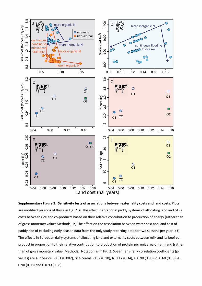
products using economic allocation, but also investigated alternative allocation rules. 144
Findings for four sectors. Our first key result is that useable data are surprisingly scarce. Few studies 145
measured paired externality and yield information, many reported externalities in substantially 146
incomplete or irreconcilably divergent ways, and we could find no suitable data at all on some 147
widely adopted practices. Nevertheless, we were able to obtain sufficient data to consider how 148
externalities vary with land costs for nine out of 20 possible sector-externality combinations 149
(Supplementary Table 1). The type of data available differed across these combinations (which we 150
view as a useful test of the flexibility of our framework). For one combination the most extensive 151
Page 9
8
data we could find was from a long-term experiment at a single location. However because we were 152
interested in generalities, where possible we used information from multiple studies – either field 153
experiments or Life Cycle Assessments (LCAs) conducted across several sites – and used Generalised 154
Linear Mixed Models (GLMMs) to correct for confounding method and site effects (Methods). Last, 155
for two sectors we used process-based models parameterised for a fixed set of conditions 156
representative of the region. 157
The data that we were able to obtain do not suggest that environmental costs are generally larger 158
for farming systems with low land costs (i.e. high-yield systems; Fig. 2). If anything, positive 159
associations – in which high-yield, land-efficient systems also have lower costs in other dimensions - 160
appear more common. For Chinese paddy rice we found sufficient multi-site experimental data to 161
explore how two focal externalities vary with land cost across contrasting systems (Methods). GHG 162
costs (Fig. 2a) showed negative associations with land cost across monoculture and rotational 163
systems (assessed separately). Our GLMMs revealed that for both system types, greater application 164
of organic N lowered land cost but increased emissions (probably because of feedstock effects on 165
the methanogenic community25
; Supplementary Table 2); in contrast there was little or no GHG 166
penalty from boosting yield using inorganic N (arrows, Fig. 2a). A large volume of data on rice and 167
water use showed weakly positive covariation in costs (Fig. 2b). GLMMs indicated that increasing 168
application of inorganic N boosted yield26
, and less irrigation lowered water use while incurring only 169
a modest yield penalty27
(Supplementary Table 2). Sensitivity tests of the rice analyses had little 170
impact on these patterns (Methods; Supplementary Fig. 2). 171
We found two useable datasets on European wheat, both from the UK (Methods). Our GLMMS of 172
data from a three-site experiment varying the N fertilisation regime revealed a complex relationship 173
between GHG and land costs (Fig. 2c; Supplementary Table 2), driven by divergent responses28
to 174
adding ammonium nitrate (which lowers land costs but increases embodied GHG emissions) and 175
Page 10
9
adding urea (which lowers land costs without increasing GHG emissions per unit production, but at 176
the cost of increased ammonia volatilisation). A single-site experiment varying inorganic N 177
treatments showed a non-linear relationship between land cost and N losses (Fig. 2d), with 178
increasing N application lowering both costs until an apparent threshold, beyond which land cost 179
decreased further but at the cost of greater N leaching (see also ref. 1). 180
In livestock systems, all data we could find showed positive covariation between land costs and 181
externalities. For Latin American beef, we located coupled yield estimates only for GHG emissions, 182
but here two different types of data (Methods) revealed a common pattern. Using GLMMs again to 183
control for potentially confounding study and site effects, we found that across multiple LCAs, 184
pasture systems with greater land demands also generated greater emissions (Fig. 2e), with both 185
land and GHG costs reduced by pasture improvements (using N fertilization or legumes). This 186
pattern across contrasting pasture systems was confirmed by running RUMINANT29
(Fig. 2f), a 187
process-based model which also identified relatively low land and GHG costs for a series of 188
silvopasture and feedlot-finishing systems (for which comparable LCA data were unavailable). 189
For European dairy, process-based modelling of three conventional and two organic systems, 190
parameterised for the UK, enabled us to estimate four different externalities alongside yield 191
(Methods). This showed that conventional systems – especially those using less grazing and more 192
concentrates – had substantially lower land and also GHG costs (Fig. 2g), in part because 193
concentrates reduce CH4 emissions from fibre digestion30
. Systems with greater use of concentrates 194
(which have less rumen-degradable protein than grass31
) also showed lower losses of N, P and soil 195
per unit production (Fig. 2h,i,j). These broad patterns persisted when we used protein production 196
rather than economic value to allocate costs to co-products (Methods; Supplementary Fig. 2). 197
Incorporating land use. As a final analysis we examined the additional externalities resulting from 198
the different land requirements of contrasting systems. To generate the same quantity of 199
Page 11
10
agricultural product, low-yield systems require more land, allowing less to be retained or restored as 200
natural habitat. This is in turn likely to increase GHG emissions and soil loss, and alter hydrology - 201
though we could only find enough data to explore the first of these effects. For each sector we 202
supplemented our direct GHG figures for each system with estimates of GHG consequences of their 203
land use following IPCC methods32
to calculate the sequestration potential of a hectare not used for 204
farming and instead allowed to revert to climax vegetation (Methods). Results (Fig. 3) showed that 205
these GHG opportunity costs of agriculture were typically greater than the emissions from farming 206
activities themselves and, when added to them, in every sector generated strongly positive across-207
system associations between overall GHG cost and land cost. These patterns were maintained in 208
sensitivity tests where we halved recovery rates or assumed half of the area potentially freed from 209
farming was retained under agriculture (Methods; Supplementary Fig. 3). These findings thus 210
confirm recent suggestions33,34
that high-yield farming has the potential, provided land not needed 211
for production is largely used for carbon sequestration, to make a substantial contribution to 212
mitigating climate change. 213
Conclusions, caveats, and knowledge gaps. This study was conceived as an exploration of whether 214
high-yield systems – central to the idea of sparing land for nature in the face of enormous human 215
demand for farm products - typically impose greater negative externalities than alternative 216
approaches. Our results support three conclusions. First, useful data are worryingly limited. We 217
considered only four relatively well-studied sectors and a narrow set of externalities - not including 218
important impacts such as soil health or the effects of pesticide exposure on human health20
. Even 219
then we found studies reporting yield-linked estimates of externalities scarce, with many widely 220
adopted or promising practices within these sectors undocumented. We were not able to examine 221
complex agricultural systems (such as mixed farming, or agroforestry) which might have relatively 222
low externalities. Relevant data on many significant developing-world farm sectors (such as cassava 223
Page 12
11
or dryland cereal production in Africa) also appear very limited. Given that a multi-dimensional 224
understanding of the environmental effects of alternative production systems is integral to 225
delivering sustainable intensification, more field measurements linking yield with a broader suite of 226
externalities across a much wider range of practices and sectors are urgently needed. 227
Second, the available data on the sector-externality combinations we considered do not suggest that 228
negative associations between land cost and other environmental costs of farming are typical (cf Fig. 229
1a). Many low-yield systems impose high costs in other ways too and, although certain yield-230
improving practices have undesirable impacts (e.g. organic fertilisation of paddy rice increasing CH4 231
emissions; see also ref. 1), other practices appear capable of reducing several costs simultaneously 232
(see also refs 1,8,24,35,36). High (but not excessive) application of inorganic N, for example, can 233
lower land take of Chinese rice production without incurring GHG or water-use penalties. Similarly, 234
in Brazilian beef production adopting better pasture management, semi-intensive silvopasture and 235
feedlot-finishing can all boost yields alongside lowering GHG emissions. It is worth noting that 236
although most systems we examined are relatively high-yielding, other recent work suggests that 237
positive associations (cf trade-offs) among environmental and land costs may if anything be more 238
likely in lower-yielding systems1. 239
Third, pursuing promising high-yield systems is clearly not the same as encouraging business-as-240
usual industrial agriculture. Some high-yield practices we did not examine, such as the heavy use of 241
pesticides in much tropical fruit cultivation37
, are likely to increase externality costs per unit 242
production. Of the high-yield practices we did investigate some, such as applying fossil-fuel-derived 243
ammonium nitrate to UK wheat, impose disproportionately high environmental costs. Others that 244
seem favourable in terms of our focal externalities incur other costs, such as high NH3 emissions 245
from using urea on wheat28
, and management regimes that reduce costs in one geographic setting 246
may not do so in others1. Much work characterising existing systems and designing new ones is thus 247
Page 13
12
needed. We suggest our framework can serve as a device for identifying existing yield-enhancing 248
systems which also lower other environmental costs – and perhaps more importantly, for 249
benchmarking the environmental performance of promising new technologies and practices. 250
We close by stressing that for high-yield systems to generate any environmental benefits they must 251
be coupled with efforts to reduce rebound effects. Several plausible mechanisms for limiting these 252
by explicitly linking yield growth to improved environmental performance have been identified – 253
including strict land-use zoning; strategic deployment of yield-enhancing loans, expertise or 254
infrastructure; conditional access to markets; and restructured rural subsidies15
. Without such 255
linkages, systems which perform well per unit production may nevertheless cause net environmental 256
harm through higher profits or lower prices stimulating land conversion38–40
, and damage human 257
health by encouraging overconsumption of cheap, calorie-rich but nutrient-deficient foods41,42,
. If 258
promising high-yield strategies are to help solve rather than exacerbate society’s challenges, yield 259
increases instead need to be combined with far-reaching demand-side interventions1,6,41
and directly 260
linked with effective measures to constrain agricultural expansion15
. 261
262
Page 14
13
Methods 263
Focal sectors and externalities. We focused on 4 globally significant farm sectors (Asian paddy rice, 264
European wheat, Latin American beef, European dairy, accounting for 90%, 33%, 23% and 53% of 265
global output of these products43
) and 5 major externalities (greenhouse gas [GHG] emissions, water 266
use, nitrogen [N], phosphorus [P] and soil losses). We chose these sector-externality combinations 267
because preliminary work suggested they were characterised quantitatively relatively often, using 268
diverse approaches (single-site experiments, multi-site experiments, Life Cycle Assessments [LCAs] 269
and process-based models), enabling us to explore the generality of our framework. We then 270
searched the literature and consulted experts to obtain paired yield and externality estimates of 271
alternative production systems in each sector, narrowing our geographic scope so that differences in 272
system performance could be reasonably attributed to management practices (rather than gross 273
variation in bioclimate or soils). Our analyses have rarely been attempted previously and have 274
complex data requirements, so we could not adopt standard procedures developed for systematic 275
reviews on topics where many studies have attempted to answer the same research question. 276
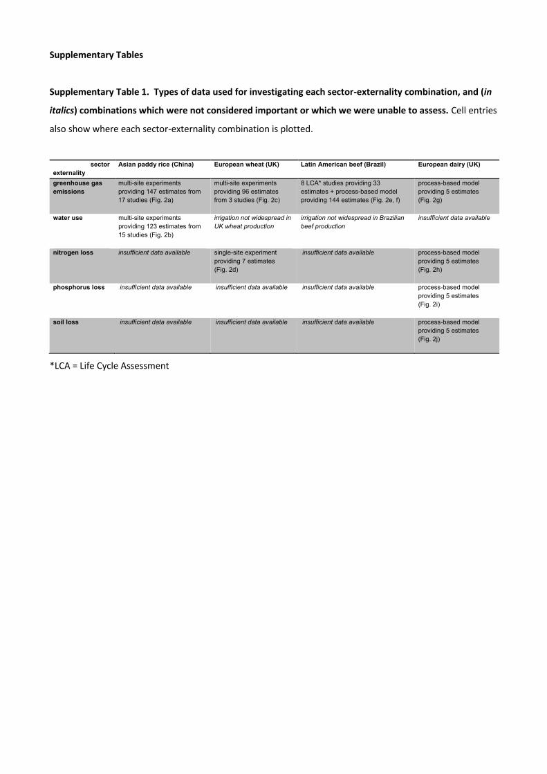
This process generated data on 5 contrasting production systems for 9 out of 20 possible sector-277
externality combinations (Supplementary Table 1): Chinese rice-GHG emissions (from multi-site 278
experiments); Chinese rice-water use (multi-site experiments); UK wheat-GHG emissions (a multi-279
site experiment); UK wheat-N emissions (a single-site experiment); Brazilian beef-GHG emissions 280
(both LCA data and process-based models); and UK dairy-GHG emissions, and N, P and soil losses 281
(process-based models). Water use in the wheat and most of the beef systems examined was limited 282
and so not explored further. We could not find sufficient paired yield-externality estimates for the 9 283
remaining sector-externality combinations. 284
The land and externality costs of each system were then expressed as total area used per unit 285
production (i.e. 1/yield) and total amount of externality generated per unit production. All estimates 286
Page 15
14
included the area used and externalities generated in producing externally-derived inputs (such as 287
feed or fertilisers). For analytical tractability, as in other recent studies1,24
we treat impacts occurring 288
at different times and places as being additive. Occasional gaps in estimates for a system were filled 289
using standard values from IPCC or other sources, or information from study authors or comparable 290
systems (details below). Where experiments or LCAs were conducted at multiple sites, we built 291
Generalised Linear Mixed Models (GLMMs) in the package lme444
in R version 3.3.145
to identify 292
effects of specific management practices on land and externality cost estimates adjusted for 293
potentially confounding biophysical and methodological effects. To illustrate the effects of 294
statistically significant management variables (those whose 95% confidence intervals did not overlap 295
zero; shown in bold in Supplementary Table 2) we estimated land and externality costs at the 296
observed minimum and maximum values (for continuous management variables) or with the 297
reference category and the category that showed the maximum effect size (for categorical 298
variables), while keeping other variables constant; we then linked these points as arrows on our 299
externality cost/land cost plots (Fig. 2 and Supplementary Figs. 1 and 2, with arrows displaced 300
horizontally and/or vertically for increased visibility). Where systems generated significant co-301
products (wheat and rapeseed from rotational rice, beef from dairy) we allocated land and 302
externality costs to the focal product in proportion to its relative contribution to the gross monetary 303
value of production per unit area of farmland (from focal and co-product combined)46
. 304
Rice and GHG emissions. Systematic searching of Scopus for experimental studies reporting both 305
yields and emissions of Chinese paddy rice systems identified 17 recently published studies47–63
306
containing 140 paired yield-emissions estimates for different systems (after within-year replicates of 307
a system were averaged). To limit confounding effects we analysed separately the data from 308
monoculture systems from southern provinces (2 rice crops per year; 5 studies, 60 estimates) and 309
rotational systems from more northerly provinces (1 rice and 1 wheat or rape crop per year; 12 310
Page 16
15
studies, 80 estimates). The studies documented the effects of variation in tillage (yes/no), 311
application rates of inorganic and organic N, and (for rotational systems only) irrigation regime 312
(continuous flooding vs episodic midseason drainage). There were insufficient data to examine 313
effects of seedling density, crop variety, organic practices, biochar application, use of groundcover to 314
lower emissions, N fertiliser type, or K or P fertilisation. 315
Land cost estimates were expressed in ha-years/tonne rice grain (i.e. the inverse of annual 316
production per hectare farmed). GHG costs were expressed in tonnes CO2eq/tonne rice grain, and 317
included CH4 and N2O emissions for growing and fallow seasons (with the latter where necessary 318
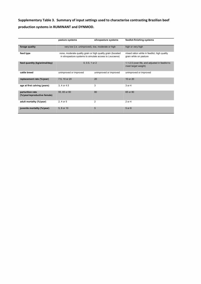
based on mean values from refs 47–49,64), and embodied emissions from N fertiliser production 319
(Yara emissions database; F. Brendrup, pers. comm.). We were unable to include emissions from 320
producing manure or K or P fertiliser, or from farm machinery. For rotational systems we adjusted 321
the land and GHG costs of rice production downwards by multiplying them by the proportional 322
contribution of rice to the gross monetary value of production per unit area of farmland from rice 323
and co-product combined (using mean post-2000 prices from ref. 43). 324
We next built GLMMs predicting variation in our estimates of land cost and GHG cost, for the 325
monoculture and rotational datasets in turn. Management practices assessed as predictors were 326
tillage regime (binary), application rates of organic N and of inorganic N, and irrigation regime 327
(binary; rotational systems only). Study site was included as a random effect. For all systems we 328
adjusted for biophysical and methodological differences across sites using the first two components 329
from a Principal Component Analysis of site scores for 14 variables: annual precipitation, 330
precipitation during the driest and wettest quarters, annual mean temperature, mean temperatures 331
during the warmest and coldest quarters, maximum temperature during the warmest month, mean 332
monthly solar radiation, latitude, longitude, soil organic carbon content, plot size, replicates per 333
estimate, and start year (with all climate data taken from refs 65,66). PCs 1 and 2 together explained 334
Page 17
16
82.3% and 76.2% of the variance in these variables for monoculture and rotational systems, 335
respectively. Soil pH and (soil pH)2 were also assessed as additional predictors. For the monoculture 336
models tolerance values were all >0.4 (indicating an absence of multicollinearity) except for the pH 337
terms (both <0.1), which we therefore removed. For the rotational models all tolerance values 338
indicated an absence of multicollinearity, but (soil pH)2 was removed because AICc values indicated 339
model fit was no better than using soil pH alone. Final models (Supplementary Table 2) were then 340
used to plot site-adjusted land and GHG costs (as points) and statistically significant management 341
effects (as arrows) in Fig. 2a. We also tested the effect of allocating land and GHG costs in rotational 342
systems based on the relative energy content of rice and co-products67
(cf relative contribution to 343
gross monetary value; Supplementary Fig. 2). 344
We adopted similar though simpler approaches for the next two sector-externality combinations, 345
which again used data from multi-site experiments. 346
Rice and water use. A systematic search on Scopus yielded 15 recent studies57,58,64,68–79
meeting our 347
criteria containing 123 paired estimates describing the effects of variation in inorganic N application 348
rate and irrigation regime on land and water costs of Chinese paddy rice. We analysed monoculture 349
and rotational systems together but considered water use solely for periods of rice production. Land 350
cost was expressed in ha-years/tonne rice grain, and water cost in m3/tonne rice grain (excluding 351
rainfall). We adjusted these estimates for site effects in GLMMs of variation in land and water costs 352
using as predictors the application rate of inorganic N, and irrigation regime (a 6-level factor: 353
continuous flooding, continuous flooding with drainage, alternate wetting and drying, controlled 354
irrigation, mulches or plastic films, and long periods of dry soil), while accounting for the effect of 355
study site as a random effect. Tolerance values were all >0.7. Final models (Supplementary Table 2) 356
were then used to plot site-adjusted land and water costs (points) and significant management 357
effects (arrows) in Fig. 2b. Almost all sources reported data on only one rice season per year, but 358
Page 18
17
one study68
included separate estimates for early- and late-season rice, so we checked the 359
robustness of our findings by re-running the analysis without the early-season data from this study 360
(Supplementary Fig. 2). 361
Wheat and GHG emissions. The Agricultural Greenhouse Gas Inventory Research Platform80–83
362
provided 96 paired measures of variation in yield and N2O emissions in response to experimental 363
changes in N fertiliser application rate and type. We expanded the emissions profile to include 364
embodied emissions from N fertiliser production (from the Yara emissions database; F. Brendrup, 365
pers. comm.). We derived land costs in ha-years/tonne wheat (at 85% dry matter) and GHG costs in 366
tonnes CO2eq/tonne wheat. Experiments were run in 3 regions, so to adjust for site effects we built 367
GLMMs of variation in land and GHG costs fitting study region as a random effect and using the 368
application rates of ammonium nitrate, urea and dicyandiamide (a nitrification inhibitor) as 369
predictors. Tolerance values were all >0.7. Adjusted land and GHG cost estimates from the final 370
models (Supplementary Table 2) are plotted in Fig. 2c, with arrows showing statistically significant 371
management practices. 372
Wheat and N losses. We assessed this sector-externality combination using data from Rothamsted’s 373
long-term Broadbalk wheat experiment, which investigates the effects of inorganic N application 374
rates on yields of winter wheat. During the 1990s changes in field drainage enabled the 375
measurement (alongside yield) of plot-specific leaching losses of nitrate84
. Mean land and N costs – 376
expressed in ha-years/tonne wheat (at 85% dry matter) and kg N leached/tonne wheat, respectively 377
– were averaged across 8 seasons (thus smoothing-out rainfall effects), for each of 7 levels of N 378
application (from 0-288 kg N [as ammonium nitrate] /ha-y; details in Fig. 2 legend). Results are 379
plotted in Fig. 2d. 380
Beef and GHG emissions. Two types of data were available for this sector-externality combination, 381
enabling us to compare findings across assessment techniques. First we examined all published LCAs 382
Page 19
18
of Brazilian beef production85–92
. Supplementing this with a bioclimatically comparable dataset from 383
tropical Mexico (R. Olea-Perez, pers. comm.) yielded 33 paired yield-emissions estimates for 384
contrasting production systems. These varied in whether they used improved pasture, 385
supplementary feeding, or improved breeds (which if unreported we inferred from age at first 386
calving, and mortality and conception rates). There were insufficient LCA data to examine the effects 387
of feedlots, silvopasture, or rotational grazing. Land costs were calculated in ha-years/tonne Carcass 388
Weight [CW], incorporating land used to grow feed, and assuming a dressing percentage of 50%93
. 389
GHG costs were derived in tonnes CO2eq/tonne CW, including enteric CH4 emissions, CH4 and N2O 390
emissions from manure, N2O emissions from managed pasture, emissions from supplementary feed 391
production (where necessary using values from ref. 86), and embodied GHG emissions from N, P 392
and K fertiliser production. There were too few data to include CO2 emissions from lime application 393
or farm machinery. Milk production was not a significant co-product. To control for site effects we 394
built GLMMs of variation in land and GHG costs using site as a random effect and use of improved 395
pasture, supplementary feeding and improved breeds (each a binary factor) as predictors. Tolerance 396
values were all >0.8. Adjusted land and GHG cost estimates from the final models (Supplementary 397
Table 2) are plotted in Fig. 2e, with arrows describing statistically significant management practices. 398
For comparison we derived an equivalent GHG cost vs land cost plot (Fig. 2f) using a process-based 399
model of beef production. RUMINANT29
is an IPCC tier 3 digestion and metabolism model which uses 400
stoichiometric equations to estimate production of meat, manure N and enteric methane for any 401
given pasture quality, supplementary feed quantity and type, cattle breed, and region. We used 402
plausible combinations of these settings (Supplementary Table 3) and corresponding values of feed 403
and forage protein, digestibility and carbohydrate content (judged representative of the Brazilian 404
beef sector by MH) to derive yield and emissions estimates for 86 contrasting pasture systems. To 405
extend beyond the scope of the LCA analyses we also modelled 50 silvopasture systems by boosting 406
Page 20
19
feed quality to simulate access to Leucaena, and 8 feedlot-finishing systems by incorporating an 83-407
120 day feedlot phase when animals received high-quality mixed ration. For each system we 408
included the whole herd, after determining the ratio of fattening:breeding animals using the 409
DYNMOD demographic projection tool94
, based on system-specific reproductive performance 410
parameters and animal growth rates (reflecting pasture quality and management; Supplementary 411
Table 3). Breeding animals experienced the same conditions as fattening animals (except that in 412
pasture and silvopasture they received no supplementary feed). Stocking rates were set to 413
sustainable carrying capacity for pasture and silvopasture, and 201 animals/ha for feedlots (DB pers. 414
obs.). Yields were converted to land cost in ha-years/tonne CW, including the area of feedlots and 415
land required to grow feed (using feed composition and yield data from refs 43,85). RUMINANT 416
emissions estimates were supplemented with estimates of manure CH4, CO2 and N2O emissions from 417
feed production, and N2O emissions from pasture fertilisation (from refs 32,85). Carbon 418
sequestration by vegetation could not be included, so we probably overestimate net GHG emissions 419
from silvopasture95
. All emissions were converted to CO2eq units (using conversion factors from refs 420
32,85 and feedlot manure distribution from ref. 96) and expressed in tonnes CO2eq/tonne CW. 421
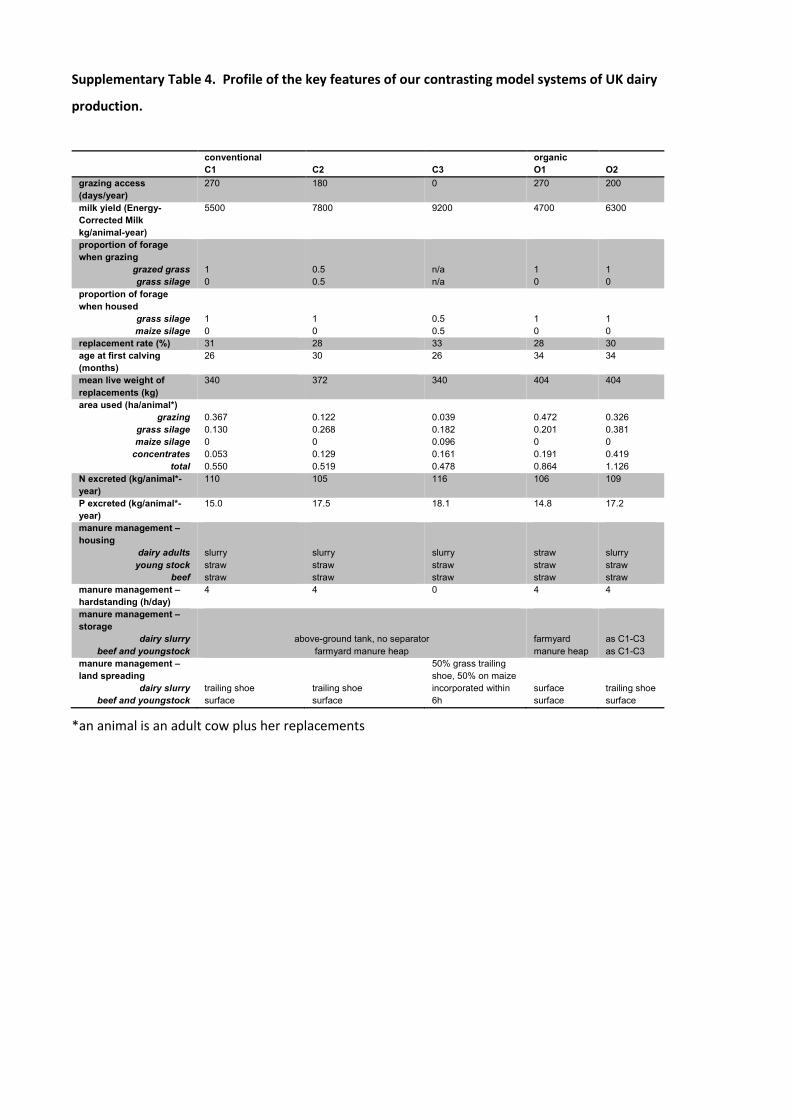
Dairy and four externalities. We also used process-based models to investigate how GHG emissions 422
and N, P and soil losses varied with land cost across 5 dairy systems representative of UK practices 423
(Supplementary Table 4; Figs. 2g-j). We modelled three conventional systems with animals accessing 424
grazing for 270, 180 and 0 days/year, and two organic systems with grazing access for 270 and 200 425
days/year. Model farms were assigned rainfall and soil characteristics based on frequency 426
distributions of these parameters for real farms of each type, with structural and management data 427
(e.g. ratios of livestock categories and ages, N and P excretion rates) based on the models of refs 428
31,97,98. Manure management was based on representative variations of the “manure 429
management continuum”99
(Supplementary Table 4). Physical performance data (annual milk yield, 430
Page 21
20
concentrate feed input, replacement rate and stocking rate) were obtained from the AHDB Dairy 431
database (M. Topliff pers. comm.) for conventional systems and from DEFRA100
for organic systems. 432
Yields were converted to land cost in ha-years/tonne Energy-Corrected Milk (ECM), including land 433
required to grow feed (from refs 101,102, with yield penalties for organic production from ref. 103). 434
Because 57% of global beef production originates from the dairy sector104
, we adjusted land costs 435
downwards by multiplying them by the proportional contribution of milk to the gross monetary 436
value of production per unit area of farmland from milk and beef combined (using prices from the 437
AHDB Dairy database (M. Topliff pers. comm.)). 438
GHG cost estimates for each system comprised CH4 emissions from enteric fermentation (based on 439
ref. 31), CH4 and N2O emissions from manure management (following refs 32 and 105), emissions 440
from N fertiliser applications to pasture (from refs 106,107), and from feed production (from ref. 441
108). Emissions from farm machinery and buildings were not included. Emissions were then summed 442
and expressed in tonnes CO2eq/tonne ECM. Nitrate losses of each system were derived from the 443
National Environment Agricultural Pollution–Nitrate (NEAP-N) model109,110
, whilst P and soil losses 444
were estimated using the Phosphorus and Sediment Yield CHaracterisation In Catchments (PSYCHIC) 445
model111,98
. These last three costs were expressed in kg/tonne ECM and (as with land costs) 446
downscaled by allocating a portion of them to beef co-products, based on milk and beef prices. 447
Finally, to check the effect of this allocation rule we re-ran each analysis instead allocating costs 448
using the relative protein content of milk and beef (from ref. 104; Supplementary Fig. 2). 449
GHG opportunity costs of land farmed. Alongside the GHG emissions generated by agricultural 450
activities themselves (analysed above), farming typically carries an additional GHG cost. Wherever 451
the carbon content of farmed land is less than that of the natural habitat that could replace it if 452
agriculture ceased, farming imposes an opportunity cost of sequestration forgone112
, whose 453
Page 22
21
magnitude increases with the area under production (and hence with the land cost of the system). 454
We quantified this GHG cost using the forgone sequestration method, whereby retaining the current 455
land use is assumed to prevent the sequestration in soils and biomass that would occur if the land 456
was allowed to revert to climax vegetation (see details in Supplementary Table 5). 457
For each forgone transition, values for annual biomass accrual ( 20 years) were taken from Table 4.9 458
of ref. 32, assuming that the climax vegetation for UK wheat and dairy was “temperate oceanic 459
forest (Europe)”, for Chinese rice it was “tropical moist deciduous forest (Asia, continental)”, and for 460
Brazilian beef it was “tropical moist deciduous forest (South America)”. The carbon content of all 461
biomass was assumed to be 47% of dry matter (ref. 32 Table 4.3). 462
Changes in soil carbon values were taken from the relevant mean percentage change in soil organic 463
carbon values for each land conversion from a global meta-analysis113
. For UK wheat and Chinese 464
rice we used values for conversion of cropland to woodland; for UK dairy and Brazilian beef we used 465
conversion of grassland to woodland for grazing land and conversion of cropland to woodland for 466
land used to grow feed. Initial soil carbon values were taken from Table 2.3 of ref. 32. We assumed 467
the soils for UK wheat were “cold temperate, moist, high activity soils”, for Chinese rice they were 468
“tropical, wet, low activity soils”, for UK dairy they were “cold temperate, moist, high activity soils” 469
for grazing land and for producing imported feed they were “subtropical humid, LAC soils” (South 470
America), and for Brazilian beef for both grazing and feed production they were “tropical, moist, low 471
activity soils”. In each case the relevant percentage change in soil organic carbon was multiplied by 472
the initial soil carbon stock to calculate an absolute change, which, following IPCC guidelines32
, we 473
assumed took 20 years. 474
Page 23
22
Total annual forgone sequestration was then estimated by adding this annual change in soil organic 475
carbon and the annual accrual of biomass carbon under reversion to climax vegetation. We assumed 476
(as in ref. 34) that each 1ha reduction in land cost results in 1ha of recovering habitat. As above, our 477
land cost estimates included land needed to produce externally-derived inputs, and (for rotational 478
rice and dairy) were adjusted downwards based on the value of co-products. These GHG opportunity 479
costs were then added to the direct GHG emissions estimates of each system, and the summed 480
values plotted against land cost (Fig. 3). 481
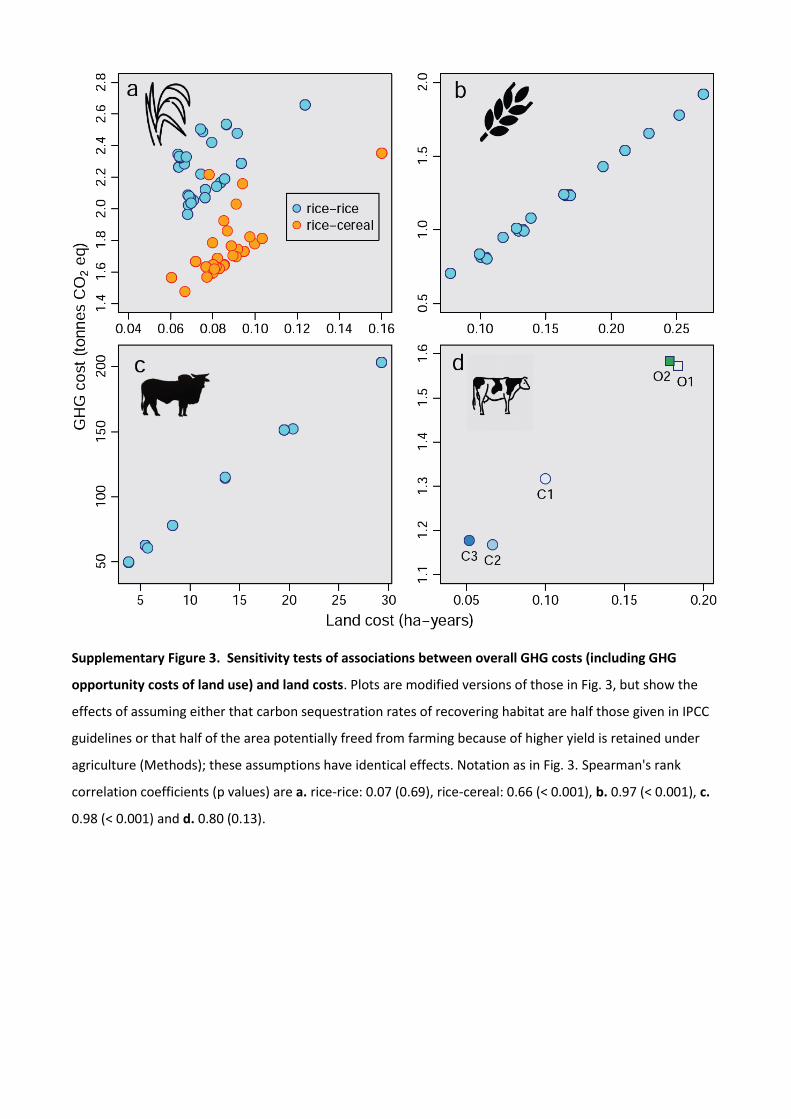
As a sensitivity test of our key assumptions we re-ran these analyses assuming that carbon recovery 482
rates are halved, or that (because of rebound or similar effects38–40
) half of the area potentially freed 483
from farming is retained under agriculture. These two changes to our assumptions have numerically 484
identical effects, shown in Supplementary Fig. 3. Note that our recovery-based estimates of the GHG 485
costs that farming imposes through land use are conservative, in that they are roughly 30-50% of 486
those obtained from calculating GHG emissions from natural habitat clearance (annualised, for 487
consistency with the recovery method, over 20 harvests; data not shown). 488
Code availability. The R codes used for the analyses are available from the corresponding author 489
upon request. 490
Data availability. The data that support the findings of this study are available from the 491
corresponding author upon request. 492
493
Page 24
23
References 494
1. Poore, J. & Nemecek, T. Reducing food’s environmental impacts through producers and 495
consumers. Science 360, 987–992 (2018). 496
2. Green, R. E., Cornell, S. J., Scharlemann, J. P. W. & Balmford, A. Farming and the fate of wild 497
nature. Science 307, 550–555 (2005). 498
3. Tilman, D., Balzer, C., Hill, J. & Befort, B. L. Global food demand and the sustainable 499
intensification of agriculture. Proc. Natl. Acad. Sci. U. S. A. 108, 20260–20264 (2011). 500
4. Hunter, M. C., Smith, R. G., Schipanski, M. E., Atwood, L. W. & Mortensen, D. A. Agriculture in 501
2050: recalibrating targets for sustainable intensification. Bioscience 67, 386–391 (2017). 502
5. Godfray, H. C. J. et al. Food security: the challenge of feeding 9 billion people. Science 327, 503
812–818 (2010). 504
6. Bajželj, B. et al. Importance of food-demand management for climate mitigation. Nat. Clim. 505
Chang. 4, 924–929 (2014). 506
7. Foley, J. A. et al. Solutions for a cultivated planet. Nature 478, 337–342 (2011). 507
8. Ripple, W. J. et al. Ruminants, climate change and climate policy. Nat. Clim. Chang. 4, 2–5 508
(2014). 509
9. Phalan, B., Onial, M., Balmford, A. & Green, R. E. Reconciling food production and biodiversity 510
conservation: land sharing and land sparing compared. Science 333, 1289–1291 (2011). 511
10. Balmford, A., Green, R. & Phalan, B. Land for food & land for nature? Daedalus 144, 57–75 512
(2015). 513
11. Hulme, M. F. et al. Conserving the birds of Uganda’s banana-coffee arc: land sparing and land 514
Page 25
24
sharing compared. PLoS One 8, e54597 (2013). 515
12. Kamp, J. et al. Agricultural development and the conservation of avian biodiversity on the 516
Eurasian steppes: a comparison of land-sparing and land-sharing approaches. J. Appl. Ecol. 52, 517
1578–1587 (2015). 518
13. Dotta, G., Phalan, B., Silva, T. W., Green, R. & Balmford, A. Assessing strategies to reconcile 519
agriculture and bird conservation in the temperate grasslands of South America: grasslands 520
conservation and agriculture. Conserv. Biol. 30, 618–627 (2016). 521
14. Williams, D. R. et al. Land-use strategies to balance livestock production, biodiversity 522
conservation and carbon storage in Yucatán, Mexico. Glob. Chang. Biol. 23, 5260–5272 523
(2017). 524
15. Phalan, B. et al. How can higher-yield farming help to spare nature? Science 351, 450–451 525
(2016). 526
16. Pretty, J. Agricultural sustainability: concepts, principles and evidence. Philos. Trans. R. Soc. 527
Lond. B. Biol. Sci. 363, 447–465 (2008). 528
17. Matson, P. A., Parton, W. J., Power, A. G. & Swift, M. J. Agricultural intensification and 529
ecosystem properties. Science 277, 504–509 (1997). 530
18. Tilman, D., Cassman, K. G., Matson, P. A., Naylor, R. & Polasky, S. Agricultural sustainability 531
and intensive production practices. Nature 418, 671–677 (2002). 532
19. Didham, R. K. et al. Agricultural intensification exacerbates spillover effects on soil 533
biogeochemistry in adjacent forest remnants. PLoS One 10, e0116474 (2015). 534
20. Seufert, V. & Ramankutty, N. Many shades of gray – the context-dependent performance of 535
organic agriculture. Sci. Adv. 3, e1602638 (2017). 536
Page 26
25
21. Kirchmann, H., Bergström, L., Kätterer, T., Andrén, O. & Andersson, R. in Organic Crop 537
Production – Ambitions and Limitations (eds. Kirchmann, H. & Bergström, L.) pp.39–72 538
(Springer, Dordrecht, The Netherlands, 2008). 539
22. Madhusudan, M. D. The global village: linkages between international coffee markets and 540
grazing by livestock in a South Indian wildlife reserve. Conserv. Biol. 19, 411–420 (2005). 541
23. Nijdam, D., Rood, T. & Westhoek, H. The price of protein: review of land use and carbon 542
footprints from life cycle assessments of animal food products and their substitutes. Food 543
Policy 37, 760–770 (2012). 544
24. Clark, M. & Tilman, D. Comparative analysis of environmental impacts of agricultural 545
production systems, agricultural input efficiency, and food choice. Environ. Res. Lett. 12, 546
64016 (2017). 547
25. Yan, X., Yagi, K., Akiyama, H. & Akimoto, H. Statistical analysis of the major variables 548
controlling methane emission from rice fields. Glob. Chang. Biol. 11, 1131–1141 (2005). 549
26. Pittelkow, C. M., Adviento-Borbe, M. A., van Kessel, C., Hill, J. E. & Linquist, B. A. Optimizing 550
rice yields while minimizing yield-scaled global warming potential. Glob. Chang. Biol. 20, 551
1382–1393 (2014). 552
27. Carrijo, D. R., Lundy, M. E. & Linquist, B. A. Rice yields and water use under alternate wetting 553
and drying irrigation: a meta-analysis. F. Crop. Res. 203, 173–180 (2017). 554
28. Smith, K. A. et al. The effect of N fertilizer forms on nitrous oxide emissions from UK arable 555
land and grassland. Nutr. Cycl. Agroecosystems 93, 127–149 (2012). 556
29. Herrero, M. et al. Biomass use, production, feed efficiencies, and greenhouse gas emissions 557
from global livestock systems. Proc. Natl. Acad. Sci. U. S. A. 110, 20888–20893 (2013). 558
Page 27
26
30. Beauchemin, K., McAllister, T. A. & McGinn, S. M. Dietary mitigation of enteric methane from 559
cattle. CAB Rev. Perspect. Agric. Vet. Sci. Nutr. Nat. Resour. 4, 1–18 (2009). 560
31. Wilkinson, J. M. & Garnsworthy, P. C. Dietary options to reduce the environmental impact of 561
milk production. J. Agric. Sci. 155, 334–347 (2017). 562
32. IPCC. 2006 IPCC Guidelines for National Greenhouse Gas Inventories, Prepared by the National 563
Greenhouse Gas Inventories Programme. (eds. Eggleston, H. S., Buendia, L., Miwa, K., Ngara, 564
T. & Tanabe, K.) (IGES, Hayama, 2006). 565
33. Gilroy, J. J. et al. Optimizing carbon storage and biodiversity protection in tropical agricultural 566
landscapes. Glob. Chang. Biol. 20, 2162–2172 (2014). 567
34. Lamb, A. et al. The potential for land sparing to offset greenhouse gas emissions from 568
agriculture. Nat. Clim. Chang. 6, 488–492 (2016). 569
35. Cui, Z. et al. Pursuing sustainable productivity with millions of smallholder farmers. Nature 570
555, 363–366 (2018). 571
36. Notarnicola, B. et al. The role of life cycle assessment in supporting sustainable agri-food 572
systems: a review of the challenges. J. Clean. Prod. 140, 399–409 (2017). 573
37. Bravo, V. et al. Monitoring pesticide use and associated health hazards in Central America. 574
Int. J. Occup. Environ. Heal. J. Int. J. Occup. Environ. Heal. 173, 1077–3525 (2011). 575
38. Lambin, E. F. & Meyfroidt, P. Global land use change, economic globalization, and the 576
looming land scarcity. Proc. Natl. Acad. Sci. U. S. A. 108, 3465–3472 (2011). 577
39. Ewers, R. M., Scharlemann, J. P. W., Balmford, A. & Green, R. E. Do increases in agricultural 578
yield spare land for nature? Glob. Chang. Biol. 15, 1716–1726 (2009). 579
Page 28
27
40. Byerlee, D., Stevenson, J. & Villoria, N. Does intensification slow crop land expansion or 580
encourage deforestation? Glob. Food Sec. 3, 92–98 (2014). 581
41. Tilman, D. & Clark, M. Global diets link environmental sustainability and human health. 582
Nature 515, 518–522 (2014). 583
42. Yang, Q. et al. Added sugar intake and cardiovascular diseases mortality among US adults. 584
JAMA Intern. Med. 174, 516 (2014). 585
586
Page 29
28
References cited exclusively in Methods 587
43. FAO. FAOSTAT: Food and Agriculture Data http://fao.org/faostat/ (Food and Agriculture 588
Organization of the Uniated Nations, Rome, 2017). 589
44. Bates, D., Mächler, M., Bolker, B. & Walker, S. Fitting linear mixed-effects models using lme4. 590
J. Stat. Softw. 67, 1–48 (2015). 591
45. R Core Team. R: A Language and Environment for Statistical Computing https://www.r-592
project.org/ (R Foundation for Statistical Computing, Vienna, Austria, 2016). 593
46. Guinée, J. B., Heijungs, R. & Huppes, G. Economic allocation: examples and derived decision 594
tree. Int. J. Life Cycle Assess. 9, 23–33 (2004). 595
47. Shang, Q. et al. Net annual global warming potential and greenhouse gas intensity in Chinese 596
double rice-cropping systems: a 3-year field measurement in long-term fertilizer experiments. 597
Glob. Chang. Biol. 17, 2196–2210 (2011). 598
48. Liu, Y. et al. Net global warming potential and greenhouse gas intensity from the double rice 599
system with integrated soil–crop system management: a three-year field study. Atmos. 600
Environ. 116, 92–101 (2015). 601
49. Chen, Z., Chen, F., Zhang, H. & Liu, S. Effects of nitrogen application rates on net annual global 602
warming potential and greenhouse gas intensity in double-rice cropping systems of the 603
Southern China. Environ. Sci. Pollut. Res. Int. 23, 24781–24795 (2016). 604
50. Xue, J. F. et al. Assessment of carbon sustainability under different tillage systems in a double 605
rice cropping system in Southern China. Int. J. Life Cycle Assess. 19, 1581–1592 (2014). 606
51. Shen, J. et al. Contrasting effects of straw and straw-derived biochar amendments on 607
greenhouse gas emissions within double rice cropping systems. Agric. Ecosyst. Environ. 188, 608
Page 30
29
264–274 (2014). 609
52. Ma, Y. C. et al. Net global warming potential and greenhouse gas intensity of annual rice-610
wheat rotations with integrated soil-crop system management. Agric. Ecosyst. Environ. 164, 611
209–219 (2013). 612
53. Zhang, X., Xu, X., Liu, Y., Wang, J. & Xiong, Z. Global warming potential and greenhouse gas 613
intensity in rice agriculture driven by high yields and nitrogen use efficiency. Biogeosciences 614
13, 2701–2714 (2016). 615
54. Yang, B. et al. Mitigating net global warming potential and greenhouse gas intensities by 616
substituting chemical nitrogen fertilizers with organic fertilization strategies in rice-wheat 617
annual rotation systems in China: a 3-year field experiment. Ecol. Eng. 81, 289–297 (2015). 618
55. Zhang, Z. S., Guo, L. J., Liu, T. Q., Li, C. F. & Cao, C. G. Effects of tillage practices and straw 619
returning methods on greenhouse gas emissions and net ecosystem economic budget in rice-620
wheat cropping systems in central China. Atmos. Environ. 122, 636–644 (2015). 621
56. Xiong, Z. et al. Differences in net global warming potential and greenhouse gas intensity 622
between major rice-based cropping systems in China. Sci. Rep. 5, 17774 (2015). 623
57. Xu, Y. et al. Improved water management to reduce greenhouse gas emissions in no-till 624
rapeseed–rice rotations in Central China. Agric. Ecosyst. Environ. 221, 87–98 (2016). 625
58. Xu, Y. et al. Effects of water-saving irrigation practices and drought resistant rice variety on 626
greenhouse gas emissions from a no-till paddy in the central lowlands of China. Sci. Total 627
Environ. 505, 1043–1052 (2015). 628
59. Yao, Z. et al. Nitrous oxide and methane fluxes from a rice-wheat crop rotation under wheat 629
residue incorporation and no-tillage practices. Atmos. Environ. 79, 641–649 (2013). 630
Page 31
30
60. Xia, L., Wang, S. & Yan, X. Effects of long-term straw incorporation on the net global warming 631
potential and the net economic benefit in a rice-wheat cropping system in China. Agric. 632
Ecosyst. Environ. 197, 118–127 (2014). 633
61. Zhang, A. et al. Change in net global warming potential of a rice-wheat cropping system with 634
biochar soil amendment in a rice paddy from China. Agric. Ecosyst. Environ. 173, 37–45 635
(2013). 636
62. Zou, J., Huang, Y., Zong, L., Zheng, X. & Wang, Y. Carbon dioxide, methane, and nitrous oxide 637
emissions from a rice-wheat rotation as affected by crop residue. Adv. Atmos. Sci. 21, 691–638
698 (2004). 639
63. Zhou, M. et al. Nitrous oxide and methane emissions from a subtropical rice-rapeseed 640
rotation system in China: a 3-year field case study. Agric. Ecosyst. Environ. 212, 297–309 641
(2015). 642
64. Yao, Z. et al. Improving rice production sustainability by reducing water demand and 643
greenhouse gas emissions with biodegradable films. Sci. Rep. 7, 39855 (2017). 644
65. Hijmans, R. J., Cameron, S. E., Parra, J. L., Jones, P. G. & Jarvis, A. WorldClim – Global Climate 645
Data: WorldClim Version 2 http://www.worldclim.org/version2 (2017). 646
66. Hijmans, R. J., Cameron, S. E., Parra, J. L., Jones, P. G. & Jarvis, A. WorldClim – Global Climate 647
Data: Bioclimatic Variables http://www.worldclim.org/bioclim (2017). 648
67. Heuzé, V., Tran, G. & Hassoun, P. Feedipedia: Rough Rice (Paddy Rice) 649
https://www.feedipedia.org/node/226 (Feedipedia, a programme by INRA, CIRAD, AFZ and 650
FAO, 2015). 651
68. Liang, K. et al. Grain yield, water productivity and CH4 emission of irrigated rice in response 652
Page 32
31
to water management in south China. Agric. Water Manag. 163, 319–331 (2016). 653
69. Kreye, C. et al. Fluxes of methane and nitrous oxide in water-saving rice production in north 654
China. Nutr. Cycl. Agroecosystems 77, 293–304 (2007). 655
70. Lu, W., Cheng, W., Zhang, Z., Xin, X. & Wang, X. Differences in rice water consumption and 656
yield under four irrigation schedules in central Jilin Province, China. Paddy Water Environ. 14, 657
473–480 (2016). 658
71. Jin, X. et al. Water consumption and water-saving characteristics of a ground cover rice 659
production system. J. Hydrol. 540, 220–231 (2016). 660
72. Sun, H. et al. CH4 emission in response to water-saving and drought-resistance rice (WDR) 661
and common rice varieties under different irrigation managements. Water, Air, Soil Pollut. 662
227, 47 (2016). 663
73. Wang, X. et al. The positive impacts of irrigation schedules on rice yield and water 664
consumption: synergies in Jilin Province, Northeast China. Int. J. Agric. Sustain. 14, 1–12 665
(2016). 666
74. Xiong, Y., Peng, S., Luo, Y., Xu, J. & Yang, S. A paddy eco-ditch and wetland system to reduce 667
non-point source pollution from rice-based production system while maintaining water use 668
efficiency. Environ. Sci. Pollut. Res. 22, 4406–4417 (2015). 669
75. Shao, G.-C. et al. Effects of controlled irrigation and drainage on growth, grain yield and water 670
use in paddy rice. Eur. J. Agron. 53, 1–9 (2014). 671
76. Liu, L. et al. Combination of site-specific nitrogen management and alternate wetting and 672
drying irrigation increases grain yield and nitrogen and water use efficiency in super rice. F. 673
Crop. Res. 154, 226–235 (2013). 674
Page 33
32
77. Chen, Y., Zhang, G., Xu, Y. J. & Huang, Z. Influence of irrigation water discharge frequency on 675
soil salt removal and rice yield in a semi-arid and saline-sodic area. Water (Switzerland) 5, 676
578–592 (2013). 677
78. Ye, Y. et al. Alternate wetting and drying irrigation and controlled-release nitrogen fertilizer in 678
late-season rice. Effects on dry matter accumulation, yield, water and nitrogen use. F. Crop. 679
Res. 144, 212–224 (2013). 680
79. Peng, S. et al. Integrated irrigation and drainage practices to enhance water productivity and 681
reduce pollution in a rice production system. Irrig. Drain. 61, 285–293 (2012). 682
80. Bell, M. J. et al. Nitrous oxide emissions from fertilised UK arable soils: fluxes, emission 683
factors and mitigation. Agric. Ecosyst. Environ. 212, 134–147 (2015). 684
81. Bell, M. J. et al. Agricultural Greenhouse Gas Inventory Research Platform - InveN2Ory: 685
Fertiliser Experimental Site in East Lothian, 2011. Version:1 [dataset] 686
https://doi.org/10.17865/ghgno606 (Freshwater Biological Association, 2017). 687
82. Cardenas, L. M., Webster, C. & Donovan, N. Agricultural Greenhouse Gas Inventory Research 688
Platform - InveN2Ory: Fertiliser Experimental Site in Bedfordshire, 2011. Version:1 [dataset] 689
https://doi.org/10.17865/ghgno613 (Freshwater Biological Association, 2017). 690
83. Williams, J.R., Balshaw, H., Bhogal, A., Kingston, H., Paine, F. & Thorman, R. E. Agricultural 691
Greenhouse Gas Inventory Research Inventory Research Platform - InveN2Ory: Fertiliser 692
Experimental Site in Herefordshire, 2011. Version:1 [dataset] 693
https://doi.org/10.17865/ghgno675 (Freshwater Biological Association, 2017. 694
84. Goulding, K. W. T., Poulton, P. R., Webster, C. P. & Howe, M. T. Nitrate leaching from the 695
Broadbalk Wheat Experiment, Rothamsted, UK, as influenced by fertilizer and manure inputs 696
Page 34
33
and the weather. Soil Use Manag. 16, 244–250 (2000). 697
85. Cardoso, A. S. et al. Impact of the intensification of beef production in Brazil on greenhouse 698
gas emissions and land use. Agric. Syst. 143, 86–96 (2016). 699
86. de Figueiredo, E. B. et al. Greenhouse gas balance and carbon footprint of beef cattle in three 700
contrasting pasture-management systems in Brazil. J. Clean. Prod. 142, 420–431 (2017). 701
87. Dick, M., Abreu Da Silva, M. & Dewes, H. Life cycle assessment of beef cattle production in 702
two typical grassland systems of southern Brazil. J. Clean. Prod. 96, 426–434 (2015). 703
88. Florindo, T. J., de Medeiros Florindo, G. I. B., Talamini, E., da Costa, J. S. & Ruviaro, C. F. 704
Carbon footprint and Life Cycle Costing of beef cattle in the Brazilian midwest. J. Clean. Prod. 705
147, 119–129 (2017). 706
89. Mazzetto, A. M., Feigl, B. J., Schils, R. L. M., Cerri, C. E. P. & Cerri, C. C. Improved pasture and 707
herd management to reduce greenhouse gas emissions from a Brazilian beef production 708
system. Livest. Sci. 175, 101–112 (2015). 709
90. Pashaei Kamali, F. et al. Environmental and economic performance of beef farming systems 710
with different feeding strategies in southern Brazil. Agric. Syst. 146, 70–79 (2016). 711
91. Ruviaro, C. F., De Léis, C. M., Lampert, V. D. N., Barcellos, J. O. J. & Dewes, H. Carbon footprint 712
in different beef production systems on a southern Brazilian farm: a case study. J. Clean. 713
Prod. 96, 435–443 (2015). 714
92. Ruviaro, C. F. et al. Economic and environmental feasibility of beef production in different 715
feed management systems in the Pampa biome, southern Brazil. Ecol. Indic. 60, 930–939 716
(2016). 717
93. Dick, M., Da Silva, M. A. & Dewes, H. Mitigation of environmental impacts of beef cattle 718
Page 35
34
production in southern Brazil - evaluation using farm-based life cycle assessment. J. Clean. 719
Prod. 87, 58–67 (2015). 720
94. Lesnoff, M. DynMod: a Tool for Demographic Projections of Tropical Livestock Populations 721
Under Microsoft Excel, User’s Manual - Version 1. (CIRAD, Montpelier, Cedex; ILRI, Nairobi, 722
Kenya, 2008). 723
95. Broom, D. M., Galindo, F. A. & Murgueitio, E. Sustainable, efficient livestock production with 724
high biodiversity and good welfare for animals. Proc. R. Soc. B. 280, 20132025 (2013). 725
96. Junior, C. C. et al. Brazilian beef cattle feedlot manure management: a country survey. J. 726
Anim. Sci. 91, 1811–1818 (2013). 727
97. Garnsworthy, P. C. The environmental impact of fertility in dairy cows: a modelling approach 728
to predict methane and ammonia emissions. Anim. Feed Sci. Technol. 112, 211–223 (2004). 729
98. Collins, A. L. & Zhang, Y. Exceedance of modern ‘background’ fine-grained sediment delivery 730
to rivers due to current agricultural land use and uptake of water pollution mitigation options 731
across England and Wales. Environ. Sci. Policy 61, 61–73 (2016). 732
99. Chadwick, D. et al. Manure management: implications for greenhouse gas emissions. Anim. 733
Feed Sci. Technol. 166–167, 514–531 (2011). 734
100. DEFRA. Organic Dairy Cows: Milk Yield and Lactation Characteristics in Thirteen Established 735
Herds and Development of a Herd Simulation Model for Organic Milk Production. Project 736
Report OF0170 737
http://randd.defra.gov.uk/Default.aspx?Menu=Menu&Module=More&Location=None&Com738
pleted=0&ProjectID=8431 (DEFRA, 2000). 739
101. Wilkinson, J. M. Re-defining efficiency of feed use by livestock. Animal 5, 1014–1022 (2011). 740
Page 36
35
102. Webb, J., Audsley, E., Williams, A., Pearn, K. & Chatterton, J. Can UK livestock production be 741
configured to maintain production while meeting targets to reduce emissions of greenhouse 742
gases and ammonia? J. Clean. Prod. 83, 204–211 (2014). 743
103. de Ponti, T., Rijk, B. & van Ittersum, M. K. The crop yield gap between organic and 744
conventional agriculture. Agric. Syst. 108, 1–9 (2012). 745
104. Gerber, P., Vellinga, T., Opio, C., Henderson, B. & Steinfeld, H. Greenhouse Gas Emissions 746
from the Dairy Sector: A Life Cycle Assessment 747
http://www.fao.org/docrep/012/k7930e/k7930e00.pdf (Food and Agriculture Organization of 748
the United Nations, Rome, 2010). 749
105. Brown, K. et al. UK Greenhouse Gas Inventory, 1990 to 2010: Annual Report for Submission 750
under the Framework Convention on Climate Change https://uk-751
air.defra.gov.uk/assets/documents/reports/cat07/1204251149_ukghgi-90-752
10_main_chapters_issue2_print_v1.pdf (DEFRA, 2012). 753
106. Misselbrook, T. H., Sutton, M. A. & Scholefield, D. A simple process-based model for 754
estimating ammonia emissions from agricultural land after fertilizer applications. Soil Use 755
Manag. 20, 365–372 (2006). 756
107. Misselbrook, T. H., Gilhespy, S. L., Cardenas, L. M., Williams, J. & Dragosits, U. Inventory of 757
Ammonia Emissions from UK Agriculture 2015: DEFRA Contract Report (SCF0102) https://uk-758
air.defra.gov.uk/assets/documents/reports/cat07/1702201346_nh3inv2015_Final_1_300920759
16.pdf (DEFRA, 2016). 760
108. Vellinga, T. V et al. Methodology Used in FeedPrint: a Tool Quantifying Greenhouse Gas 761
Emissions of Feed Production and Utilization, Report 674. (Wageningen UR Livestock 762
Research, Lelystad, The Netherlands, 2013). 763
Page 37
36
109. Anthony, S., Quinn, P. & Lord, E. Catchment scale modelling of nitrate leaching. Asp. Appl. 764
Biol. 46, 23–32 (1996). 765
110. Wang, L. et al. The changing trend in nitrate concentrations in major aquifers due to historical 766
nitrate loading from agricultural land across England and Wales from 1925 to 2150. Sci. Total 767
Environ. 542, 694–705 (2016). 768
111. Davison, P. S., Lord, E. I., Betson, M. J. & Strömqvist, J. PSYCHIC – A process-based model of 769
phosphorus and sediment mobilisation and delivery within agricultural catchments. Part 1: 770
Model description and parameterisation. J. Hydrol. 350, 290–302 (2008). 771
112. Koponen, K. & Soimakallio, S. Foregone carbon sequestration due to land occupation - the 772
case of agro-bioenergy in Finland. Int. J. Life Cycle Assess. 20, 1544–1556 (2015). 773
113. Guo, L. B. & Gifford, R. M. Soil carbon stocks and land use change: a meta analysis. Glob. 774
Chang. Biol. 8, 345–360 (2002). 775
776
777
Page 38
37
Acknowledgements We are grateful for funding from the Cambridge Conservation Initiative 778
Collaborative Fund and Arcadia, the Grantham Foundation for the Protection of the Environment, 779
the Kenneth Miller Trust the UK-China Virtual Joint Centre for Agricultural Nitrogen (CINAg, 780
BB/N013468/1, financed by the Newton Fund via BBSRC and NERC), BBSRC (BBS/E/C/000I0330), 781
DEVIL (NE/M021327/1), U-GRASS (NE/M016900/1), Soils-R-GRREAT (NE/P019455/1), N-Circle 782
(BB/N013484/1), BBSRC Soil to Nutrition (S2N) strategic programme (BBS/E/C/000I0330), UNAM-783
PAPIIT ( IV200715), the Belmont Forum/FACEE-JPI (NE/M021327/1 ‘DEVIL’), and the Cambridge 784
Earth System Science NERC DTP (NE/L002507/1); AB is supported by a Royal Society Wolfson 785
Research Merit award. Rice and wheat icons made by Freepik from www.flaticom.com. We thank 786
Frank Brendrup, Emma Caton, Achim Dobermann, Thiago Jose Florindo, Ellen Fonte, Ottoline Leyser, 787
Andre Mazzetto, Jemima Murthwaite, Farahnaz Pashaei Kamali, Rafael Olea-Perez, Stephen 788
Ramsden, Claudio Ruviaro, Jonathan Storkey, Bernardo Strassburg, Mark Topliff, Joao Nunes Vieira 789
da Silva, David Williams, Xiaoyuan Yan and Yusheng Zhang for advice, data or analysis, and to Kate 790
Willott for much practical support. 791
792
Author Contributions AB, TA, HB, DC, DE, RF, PG, RG, PS, HW, AW and RE designed the study and 793
performed the research, DMB, AC, JC, TF, EG, AG-H, JHM, MH, FH, AL, TM, BP, BIS, TT, JV and EzE 794
contributed and analysed data and results, and all authors contributed substantially to the analysis 795
and interpretation of results and writing of the manuscript. 796
797
Author Information The authors declare no competing financial interests. Correspondence and 798
requests for materials should be addressed to AB ([email protected] ). 799
800
Page 39
38
Figure Legends 801
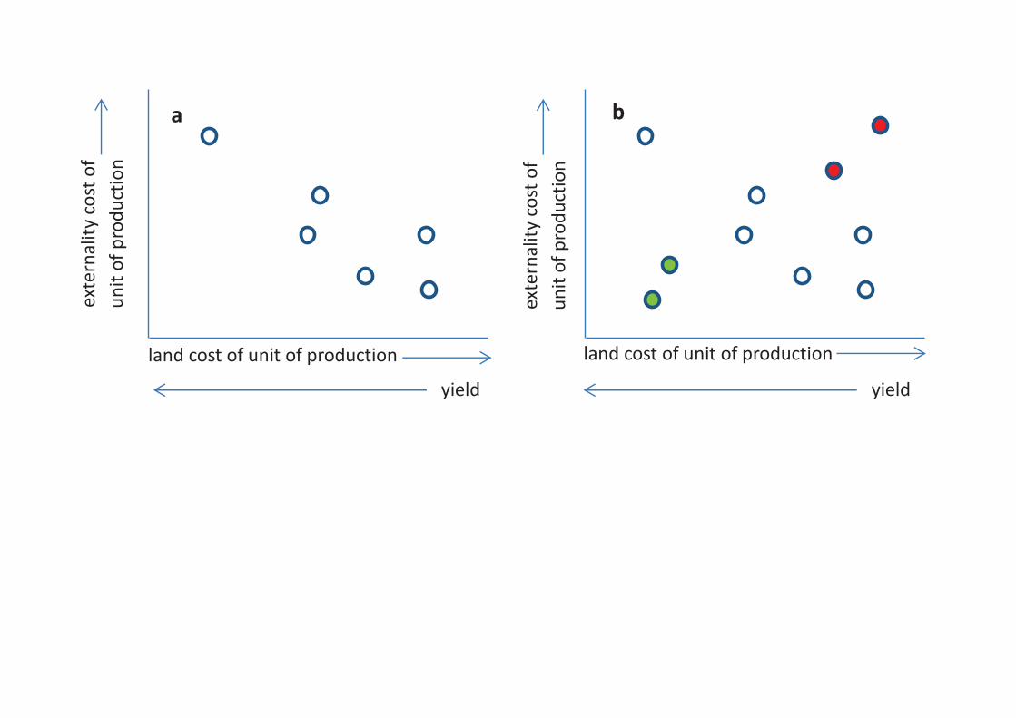
Fig. 1 | Framework for exploring how different environmental costs compare across alternative 802
production systems. a, Hypothetical plot of externality cost vs land cost of different, potentially 803
interchangeable production systems (blue circles) in a given farming sector. In this example the data 804
suggest a trade-off between externality and land costs across different systems. b, This example 805
reveals a more complex pattern, with additional systems (in green and red circles) that are low or 806
high in both costs. 807
808
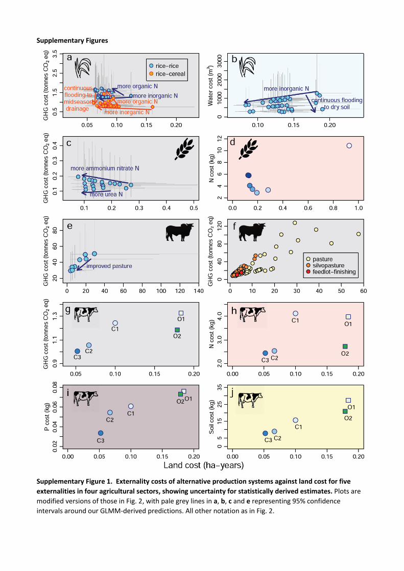
Fig. 2 | Externality costs of alternative production systems against land cost for five externalities in 809
four agricultural sectors. All costs are expressed per tonne of production (so land cost, for instance, 810
is in ha-years/tonne – i.e. the inverse of yield). Different externalities are indicated by background 811
shading (grey = GHG emissions, blue = water use, pink = N emissions, purple = P emissions, buff = soil 812
loss), and different sectors (Asian paddy rice, European wheat, Latin American beef, European dairy) 813
are shown by icons. Points on plots derived from multi-site experiments (a, b, c) and LCAs (e) show 814
values for systems adjusted for site and study effects via GLMMs of land cost and externality cost 815
(for 95% confidence intervals, see Supplementary Fig . 1), while arrows show management practices 816
with statistically-significant effects (whose 95% confidence intervals do not overlap zero in the 817
GLMMs; Methods). In d (wheat and N emissions), progressively darker circles depict increasing 818
nitrate application rate (0, 48, 96, 144, 192, 240 and 288 kg N/ha-year). In f (beef and GHG 819
emissions, estimated by RUMINANT), different colours show different system types. In g-j (dairy and 820
four externalities), circles and squares show results for conventional and organic systems, 821
respectively (detailed in Supplementary Table 4). Spearman's rank correlation coefficients (p-values) 822
are a. rice-rice: -0.51 (0.002), rice-cereal: -0.36 (0.06), b. 0.19 (0.26), c. -0.34 (0.14), d. -0.21 (0.66), e. 823
Page 40
39
0.95 (0.001), f. 0.83 (< 0.001), g. 0.90 (0.08), h. 0.70 (0.23), i. 1.00 (0.02) and j. 1.00 (0.02). Note that 824
these correlation coefficients do not necessarily reflect non-linear relationships (e.g., d) accurately. 825
826
Fig. 3 | Overall GHG cost against land cost of alternative systems in each sector, including the GHG 827
opportunity costs of land under farming. Y-axis values are the sum of GHG emissions from farming 828
activities (plotted in Figs. 2 a, c, e, g) and the forgone sequestration potential of land maintained 829
under farming and thus unable to revert to natural vegetation (Methods). All costs are expressed per 830
tonne of production. Notation as in Fig. 2. Spearman's rank correlation coefficients (p-values) are a. 831
rice-rice: 0.40 (0.017), rice-cereal: 0.80 (< 0.001), b. 0.99 (< 0.001), c. 0.98 (< 0.001) and d. 0.80 832
(0.13). 833
Page 41
ext
ern
ali
ty c
ost
of
un
it o
f p
rod
uct
ion
ext
ern
ali
ty c
ost
of
un
it o
f p
rod
uct
ion
land cost of unit of production land cost of unit of production
yield yield
a b
Page 42
0.05 0.10 0.15
0.6
1.0
1.4
1.8
GH
G c
ost
(to
nn
es C
O2 e
q)
more inorganic N
more organic N
more inorganic N
more organic N
continuousflooding tomidseasondrainage
r rice
r
a
0.08 0.10 0.12 0.14 0.16 0.18
20
06
00
10
00
14
00
Wa
ter
co
st
(m3) more inorganic N
continuous floodingto dry soil
b
0.10 0.15 0.20 0.25
0.1
00
.14
0.1
80
.22
GH
G c
ost
(to
nn
es C
O2 e
q)
more ammonium nitrate N
more urea N
c
0.0 0.2 0.4 0.6 0.8 1.02
46
81
01
2
N c
ost
(kg
)
d
5 10 15 20 25 30
25
35
45
55
GH
G c
ost
(to
nn
es C
O2 e
q)
improved pasture
e
0 10 20 30 40 50 60
04
08
01
20
GH
G c
ost
(to
nn
es C
O2 e
q)
pasturesilvopasturef
f
0.05 0.10 0.15 0.20
0.9
1.1
1.3
GH
G c
ost
(to
nn
es C
O2 e
q)
C1
C2C3
O1
O2
g
0.00 0.05 0.10 0.15 0.20
2.0
3.0
4.0
N c
ost
(kg
) C1
C2C3
O1
O2
0.00 0.05 0.10 0.15 0.20
0.0
20
.04
0.0
60
.08
P c
ost
(kg
)
C1C2
C3
O1O2
i
0.00 0.05 0.10 0.15 0.20
05
15
25
35
So
il co
st
(kg
)
C1
C2C3
O1
O2
j
years)
Page 43
0.05 0.10 0.15
2.0
2.5
3.0
3.5
4.0
r rice
r
0.10 0.15 0.20 0.25
1.0
1.5
2.0
2.5
3.0
3.5
4.0
b
5 10 15 20 25 30
50
100
150
200
250
300
350 c
0.05 0.10 0.15 0.20
1.2
1.4
1.6
1.8
2.0
C1
C2
C3
O1
O2d
y
CO2
Page 44
Supplementary information for
The environmental costs and benefits of high-yield farming
Balmford, A., T. Amano, H. Bartlett, D. Chadwick, A. Collins, D. Edwards, R. Field, P. Garnsworthy, R. Green, P.
Smith, H. Waters, A. Whitmore, D.M. Broom, J. Chara, T. Finch, E. Garnett, A. Gathorne-Hardy, J. Hernandez-
Medrano, M. Herrero, F. Hua , A. Latawiec, T. Misselbrook, B. Phalan, B. I. Simmons, T. Takahashi, J. Vause, E.
zu Ermgassen & R. Eisner.
Page 45
Supplementary Figures
Supplementary Figure 1. Externality costs of alternative production systems against land cost for five
externalities in four agricultural sectors, showing uncertainty for statistically derived estimates. Plots are
modified versions of those in Fig. 2, with pale grey lines in a, b, c and e representing 95% confidence
intervals around our GLMM-derived predictions. All other notation as in Fig. 2.
Page 46
Supplementary Figure 2. Sensitivity tests of associations between externality costs and land costs. Plots
are modified versions of those in Fig. 2. a, The effect in rotational paddy systems of allocating land and GHG
costs between rice and co-products based on their relative contribution to production of energy (rather than
of gross monetary value; Methods). b, The effect on the association between water cost and land cost of
paddy rice of excluding early-season data from the only study reporting data for two seasons per year. c-f,
The effects in European dairy systems of allocating land and externality costs between milk and its beef co-
product in proportion to their relative contribution to production of protein per unit area of farmland (rather
than of gross monetary value; Methods). Notation as in Fig. 2. Spearman's rank correlation coefficients (p-
values) are a. rice-rice: -0.51 (0.002), rice-cereal: -0.32 (0.10), b. 0.17 (0.34), c. 0.90 (0.08), d. 0.60 (0.35), e.
0.90 (0.08) and f. 0.90 (0.08).
Page 47
Supplementary Figure 3. Sensitivity tests of associations between overall GHG costs (including GHG
opportunity costs of land use) and land costs. Plots are modified versions of those in Fig. 3, but show the
effects of assuming either that carbon sequestration rates of recovering habitat are half those given in IPCC
guidelines or that half of the area potentially freed from farming because of higher yield is retained under
agriculture (Methods); these assumptions have identical effects. Notation as in Fig. 3. Spearman's rank
correlation coefficients (p values) are a. rice-rice: 0.07 (0.69), rice-cereal: 0.66 (< 0.001), b. 0.97 (< 0.001), c.
0.98 (< 0.001) and d. 0.80 (0.13).
Page 48
Supplementary Tables
Supplementary Table 1. Types of data used for investigating each sector-externality combination, and (in
italics) combinations which were not considered important or which we were unable to assess. Cell entries
also show where each sector-externality combination is plotted.
sector
externality
Asian paddy rice (China) European wheat (UK) Latin American beef (Brazil) European dairy (UK)
greenhouse gas
emissions
multi-site experiments
providing 147 estimates from
17 studies (Fig. 2a)
multi-site experiments
providing 96 estimates
from 3 studies (Fig. 2c)
8 LCA* studies providing 33
estimates + process-based model
providing 144 estimates (Fig. 2e, f)
process-based model
providing 5 estimates
(Fig. 2g)
water use multi-site experiments
providing 123 estimates from
15 studies (Fig. 2b)
irrigation not widespread in
UK wheat production
irrigation not widespread in Brazilian
beef production
insufficient data available
nitrogen loss insufficient data available single-site experiment
providing 7 estimates
(Fig. 2d)
insufficient data available process-based model
providing 5 estimates
(Fig. 2h)
phosphorus loss insufficient data available insufficient data available insufficient data available process-based model
providing 5 estimates
(Fig. 2i)
soil loss insufficient data available insufficient data available insufficient data available process-based model
providing 5 estimates
(Fig. 2j)
*LCA = Life Cycle Assessment
Page 49
Supplementary Table 2. Details of Generalised Linear Mixed Models for the effect of management
variables and covariates on land and externality costs. Estimated coefficients are shown; those whose 95%
confidence intervals (in parentheses) did not overlap zero are in bold. Tillage in Rice-GHG models represents
the effect of a tillage regime (compared to a no-tillage regime). Irrigation in Rice-GHG models is for the effect
of episodic midseason drainage compared to continuous flooding. The effect of irrigation in Rice-Water
models is based on five levels compared to continuous flooding: continuous flooding with a drainage (CF-
drain), alternative wetting and drying (AWD), controlled irrigation (CI), mulches or plastic films (F-M) and
long periods of dry soil (Dry). In Beef-GHG models, improved breed represents the effect of using an
improved breed relative to an unimproved breed. Cell entries also show where the results of each GLMM
are plotted.
Model Coefficients
Rice - GHG Inorganic N Organic N Tillage PC1 PC2
monoculture
n = 60
# studies = 5
Land cost -1.53 × 10⁻³
(-2.13 × 10⁻³, -0.94 × 10⁻³)
-1.43 × 10⁻³
(-2.35 × 10⁻³, -0.50 × 10⁻³)
-0.061
(-0.23, 0.11)
-0.052
(-0.071, -0.033)
0.038
(0.0026, 0.074)
(Fig. 2a) Externality cost
-0.20 × 10⁻³
(-1.08 × 10⁻³, 0.69 × 10⁻³)
1.76 × 10⁻³
(0.39 × 10⁻³, 3.12 × 10⁻³)
0.19
(-0.062, 0.45)
-0.12
(-0.15, -0.092)
-0.029
(-0.082, 0.023)
Inorganic N Organic N Tillage Irrigation Soil pH PC1 PC2
rotational
n = 80
# studies = 12
Land cost -1.46 × 10⁻³
(-1.70 × 10⁻³, -1.22 × 10⁻³)
-0.89 × 10⁻³
(-1.54 × 10⁻³, -0.25 × 10⁻³)
0.023
(-0.27, 0.31)
-0.018
(-0.21, 0.18)
0.081
(-0.016, 0.18)
-0.015
(-0.062, 0.032)
-0.022
(-0.068, 0.023)
(Fig. 2a) Externality cost
1.28 × 10⁻⁴
(-3.34 × 10⁻⁴, 5.95 × 10⁻⁴)
1.56 × 10⁻³
(0.32 × 10⁻³, 2.74 × 10⁻³)
-0.083
(-0.65, 0.45)
-0.51
(-0.89, -0.13)
0.086
(-0.038, 0.21)
-0.094
(-0.17, -0.011)
0.016
(-0.047, 0.081)
rotational
with energy allocation
Land cost -1.45 × 10⁻³
(-1.69 × 10⁻³, -1.20 × 10⁻³)
-0.95 × 10⁻³
(-1.60 × 10⁻³, -0.30 × 10⁻³)
-0.0084
(-0.30, 0.28)
-0.020
(-0.22, 0.17)
0.11
(0.012, 0.22)
-0.037
(-0.086, 0.011)
-0.013
(-0.063, 0.034)
(Supplementary Fig. 2a)
Externality cost
1.62 × 10⁻⁴
(-2.62 × 10⁻⁴, 6.13 × 10⁻⁴)
1.50 × 10⁻³
(0.29 × 10⁻³, 2.58 × 10⁻³)
-0.14
(-0.71, 0.43)
-0.52
(-0.90, -0.17)
0.11
(-0.032, 0.26)
-0.11
(-0.20, -0.028)
0.032
(-0.044, 0.10)
Rice – Water Inorganic N Irrigation
CF-drain
Irrigation
AWD
Irrigation
CI
Irrigation
F-M
Irrigation
Dry Rainfall
n = 123
# studies = 15
Land cost -1.68 × 10⁻³
(-2.02 × 10⁻³, -1.33 × 10⁻³)
0.021
(-0.056, 0.098)
-0.0076
(-0.066, 0.051)
0.088
(-0.010, 0.19)
0.041
(-0.071, 0.15)
0.066
(-0.039, 0.17)
-0.70 × 10⁻⁴
(-2.66 × 10⁻⁴, 1.21 × 10⁻⁴)
(Fig. 2b) Externality cost
-1.26 × 10⁻³
(-2.64 × 10⁻³, 0.13 × 10⁻³)
-0.095
(-0.41, 0.22)
-0.53
(-0.76, -0.28)
-0.88
(-1.28, -0.48)
-1.12
(-1.58, -0.65)
-1.29
(-1.72, -0.87)
-1.12 × 10⁻³
(-1.90 × 10⁻³, -0.35 × 10⁻³)
excluding three records in ref. 68
Land cost -1.67 × 10⁻³
(-2.02 × 10⁻³, -1.32 × 10⁻³)
0.023
(-0.057, 0.10)
-0.0066
(-0.068, 0.055)
0.089
(-0.011, 0.19)
0.042
(-0.072, 0.16)
0.067
(-0.040, 0.17)
-1.02 × 10⁻⁴
(-3.94 × 10⁻⁴, 1.87 × 10⁻⁴)
n = 120
# studies = 15
(Supplementary Fig. 2b)
Externality cost
-1.41 × 10⁻³
(-2.73 × 10⁻³, -0.068 × 10⁻³)
-0.14
(-0.44, 0.17)
-0.53
(-0.77, -0.30)
-0.92
(-1.31, -0.54)
-1.19
(-1.64, -0.74)
-1.32
(-1.72, -0.91)
0.28 × 10⁻³
(-0.82 × 10⁻³, 1.38 × 10⁻³)
Wheat - GHG Ammonium N rate
Urea N rate dicyandiamide rate
n = 96
# regions = 3
Land cost -4.17 × 10⁻³
(-4.87 × 10⁻³, -3.47 × 10⁻³)
-3.97 × 10⁻³
(-4.92 × 10⁻³, -3.02 × 10⁻³)
-0.0035
(-0.011, 0.0039)
(Fig. 2c) Externality cost
1.10 × 10⁻³
(0.25 × 10⁻³, 1.94 × 10⁻³)
-0.37 × 10⁻³
(-1.51 × 10⁻³, 0.77 × 10⁻³)
-0.0080
(-0.017, 0.00086)
Page 50
Beef – GHG (empirical)
Improved breed
Supplementary feed
Improved pasture
n = 33
# studies = 8
Land cost -0.41
(-1.01, 0.19)
-0.36
(-0.92, 0.20)
-1.26
(-1.81, -0.68)
(Fig. 2e) Externality cost
-0.022
(-0.26, 0.23)
-0.14
(-0.34, 0.071)
-0.38
(-0.57, -0.17)
Page 51
Supplementary Table 3. Summary of input settings used to characterise contrasting Brazilian beef
production systems in RUMINANT and DYNMOD.
pasture systems silvopasture systems feedlot-finishing systems
forage quality very low (i.e. unimproved), low, moderate or high high or very high
feed type none, moderate quality grain or high quality grain (boosted
in silvopasture systems to simulate access to Leucaena)
mixed ration while in feedlot, high quality
grain while on pasture
feed quantity (kg/animal/day) 0, 0.5, 1 or 2 1.1-2.5 (over life, and adjusted in feedlot to
meet target weight)
cattle breed unimproved or improved unimproved or improved unimproved or improved
replacement rate (%/year) 7.5, 10 or 20 20 10 or 20
age at first calving (years) 3, 4 or 4.5 3 3 or 4
parturition rate
(%/year/reproductive female)
55, 65 or 80 80 65 or 80
adult mortality (%/year) 2, 4 or 5 2 2 or 4
juvenile mortality (%/year) 5, 8 or 10 5 5 or 8
Page 52
Supplementary Table 4. Profile of the key features of our contrasting model systems of UK dairy
production.
conventional
C1
C2
C3
organic
O1
O2
grazing access
(days/year)
270 180 0 270 200
milk yield (Energy-
Corrected Milk
kg/animal-year)
5500 7800 9200 4700 6300
proportion of forage
when grazing
grazed grass
grass silage
1
0
0.5
0.5
n/a
n/a
1
0
1
0
proportion of forage
when housed
grass silage
maize silage
1
0
1
0
0.5
0.5
1
0
1
0
replacement rate (%) 31 28 33 28 30
age at first calving
(months)
26 30 26 34 34
mean live weight of
replacements (kg)
340 372 340 404 404
area used (ha/animal*)
grazing
grass silage
maize silage
concentrates
total
0.367
0.130
0
0.053
0.550
0.122
0.268
0
0.129
0.519
0.039
0.182
0.096
0.161
0.478
0.472
0.201
0
0.191
0.864
0.326
0.381
0
0.419
1.126
N excreted (kg/animal*-
year)
110 105 116 106 109
P excreted (kg/animal*-
year)
15.0 17.5 18.1 14.8 17.2
manure management –
housing
dairy adults
young stock
beef
slurry
straw
straw
slurry
straw
straw
slurry
straw
straw
straw
straw
straw
slurry
straw
straw
manure management –
hardstanding (h/day)
4 4 0 4 4
manure management –
storage
dairy slurry
beef and youngstock
above-ground tank, no separator
farmyard manure heap
farmyard
manure heap
as C1-C3
as C1-C3
manure management –
land spreading
dairy slurry
beef and youngstock
trailing shoe
surface
trailing shoe
surface
50% grass trailing
shoe, 50% on maize
incorporated within
6h
surface
surface
trailing shoe
surface
*an animal is an adult cow plus her replacements
Page 53
Supplementary Table 5. Sources of values used to estimate the rate of accumulation of above- and below-
ground carbon when farmland recovers to natural habitat.
variable value(s) used source
rate of recovery of above-ground biomass (tonnes
dry matter/ha-year)
domain-, ecosystem- and continent-specific
values
Table 4.9 in ref. 32
carbon content of biomass (tonnes C/tonne dry
matter)
0.47 Table 4.3 in ref. 32
soil carbon content of natural habitat (tonnes C/ha) climate- and soil-specific values Table 2.3 in ref. 32
proportional change in soil carbon upon land-use
transition
transition-specific values Ref. 113