58
Bandpass filters and Hilbert Transform Summary of Chapter 14 In Analyzing Neural Time Series Data: Theory and Practice Lauritz W. Dieckman
| Date post: | 31-Jul-2018 |
| Category: |
Documents |
| Upload: | truongkhanh |
| View: | 216 times |
| Download: | 0 times |

Bandpass filtersand
Hilbert Transform
Summary of Chapter 14 In
Analyzing Neural Time Series Data:Theory and PracticeLauritz W. Dieckman

A quick message from Mike X
I've created a googlegroups for the book. If you have other questions about the book, analyses, or code, feel free to post them there.
https://groups.google.com/forum/#!forum/analyzingneuraltimeseriesdata
Filters ‐Everywhere
• Music‐analog recordings~44,100 Hz sampling‐typically bandpassfiltered to rangeof human hearing‐Or, purposefully Used in artistic creation‐One persons distortion is another persons art

Why? Filter‐Hilbert Method vs
Complex Wavelet ConvolutionSimilarities• Used to create a complex (real and imaginary) time series (analytic signal) from real signal data
• Analytic signal used to determine phase and power
‐Methods described in Chapter 13• The signal must be bandpass filtered before

Why? Filter‐Hilbert Method vs
Complex Wavelet ConvolutionDifferences• Signal must first be bandpass filtered• Analytic signal acquired by creating the “phase quadrature
component” (one quarter‐cycle) by rotating sections of a Fourier spectrum.
• PRO: Filter‐Hilbert provides superior control over frequency filtering ‐not limited in shape whereas bandpass filters can take many shapes
• CON: However, Filter‐Hilbert requires signal processing toolbox for kernel creation (unlike Morlet wavelets).
• CON: Bandpass filtering is slower than wavelets

Bandpass Filtering
• First step is Bandpass filtering ‐Don’t worry Hilbert fans, we’ll get back to Hilbert transform soon
• Highly recommended to separate frequencies before the transform ‐e.g. lower frequencies may dominate combined signal
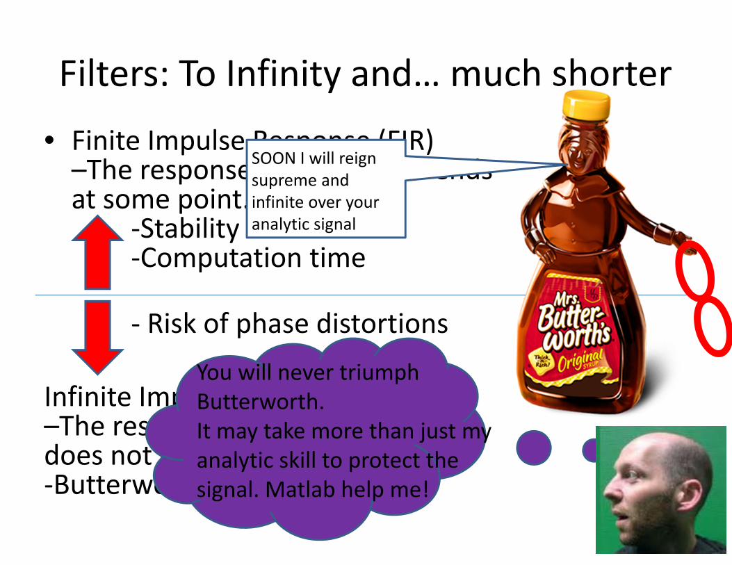
Filters: To Infinity and… much shorter
• Finite Impulse Response (FIR) –The response to an impulse ends at some point.
‐Stability‐Computation time
‐ Risk of phase distortions
Infinite Impulse Response (IIR) –The response to an impulsedoes not end.‐Butterworth IIR filter
You will never triumph Butterworth.It may take more than just my analytic skill to protect the signal. Matlab help me!
SOON I will reign supreme and infinite over your analytic signal

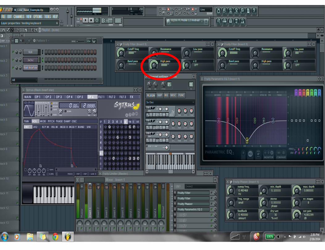
Filters: Types• High‐pass filter – Allows frequencies higher than cutoff to remain in the signal (lower frequency signals are attenuated)‐Simple illustration – Cutoff 5
1 2 3 4 5 6 7 8

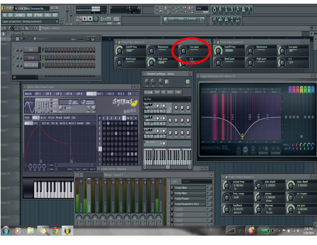
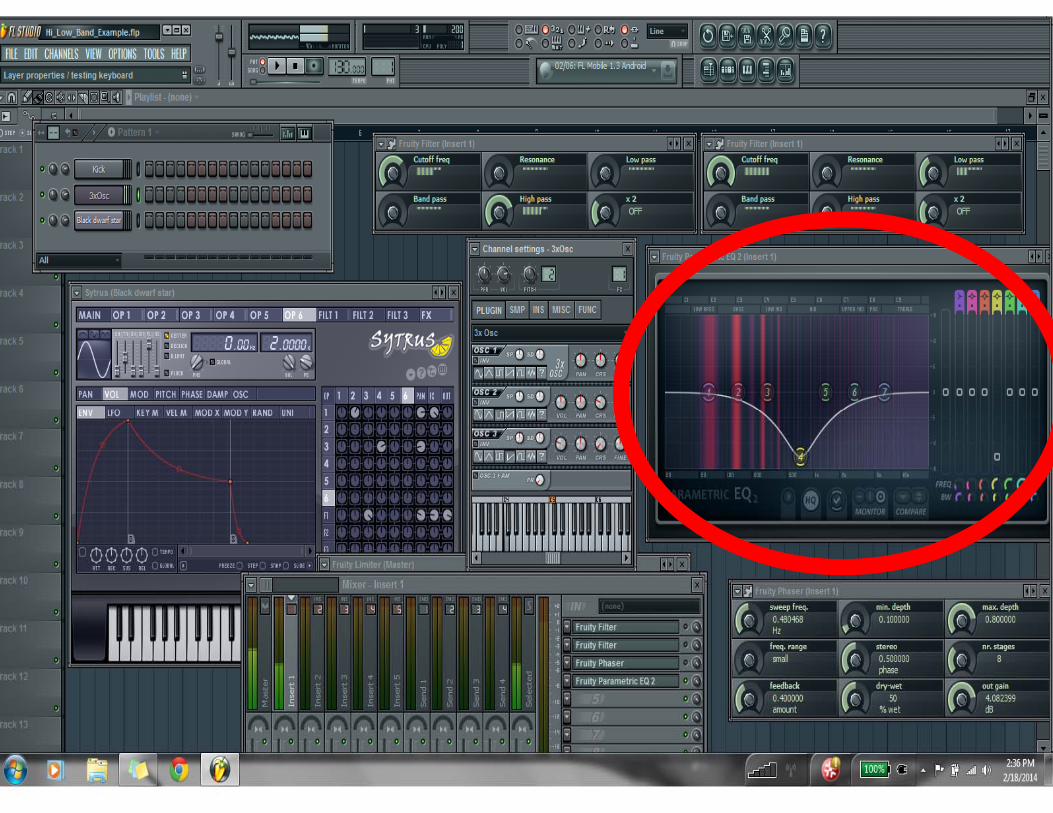
FL studio example

• Low‐pass filter – Allows frequencies lower than cutoff to remain in the signal (higher frequency signals are attenuated)‐Simple illustration – Cutoff 5
1 2 3 4 5 6 7 8
Filters: Types

• Band‐Stop filter – Attenuates or removes frequencies within a specific range. ‐e.g. Notch filters at 60 Hz
‐Simple illustration – Low Cutoff 5 & High Cutoff 2
1 2 3 4 5 6 7 8
Filters: Types

• Bandpass filter – Allows frequencies lower than lower bound cutoff to remain in the signal and frequencies higher than higher bound cut off to remain in the signal
‐Simple illustration – Low Cutoff 5 & High Cutoff 21 2 3 4 5 6 7 8‐Basically a high and low‐pass combo
Filters: Types
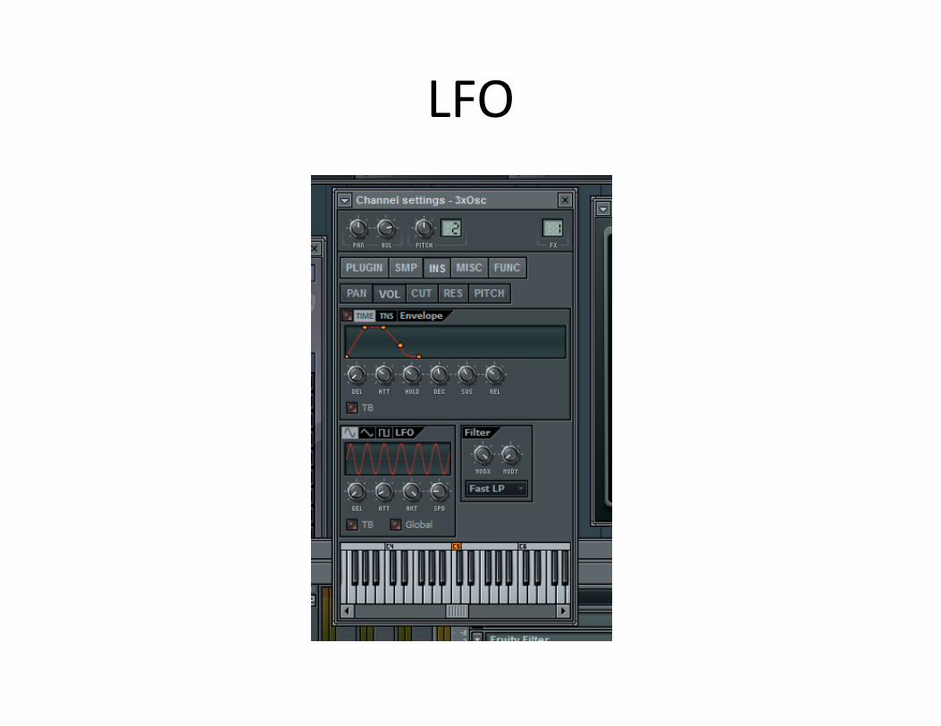
LFO

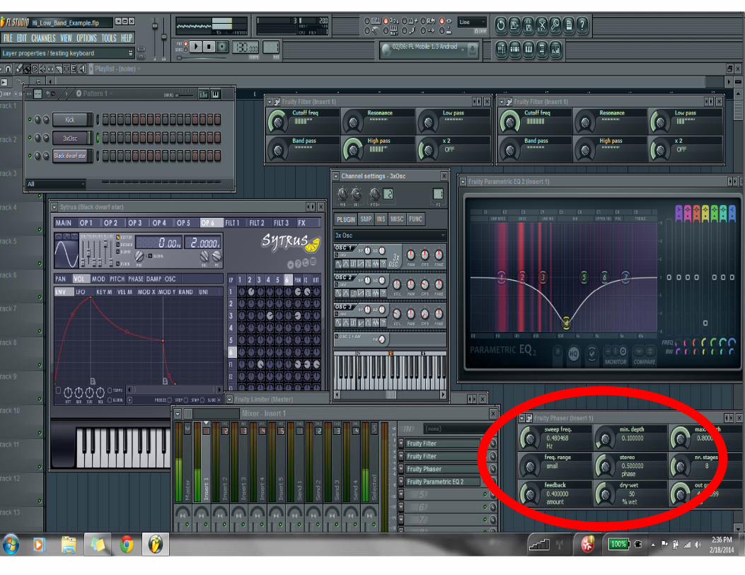
Many Music FX use filters Filter• Phaser‐Separates signal 1. Unfiltered2. Alters phase‐When recombined the signals out of phase nullify‐Frequently combined with low frequency ossiclator

How to: Filter Kernel Construction
• Like complex wavelet convolution – The analytic signal produced from filtering *weighted combination of kernel and signal
How to: Filter Kernel Construction
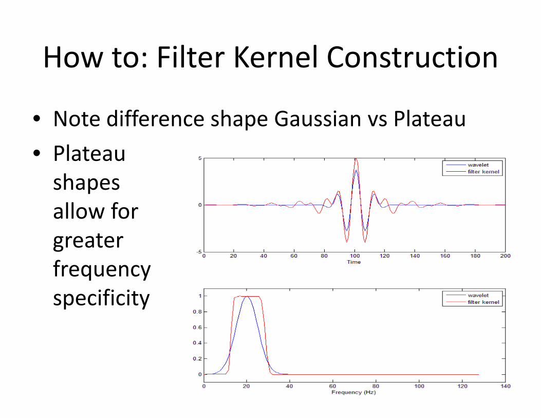
• Note difference shape Gaussian vs Plateau• Plateau shapes allow for greater frequency specificity
Filter Functions
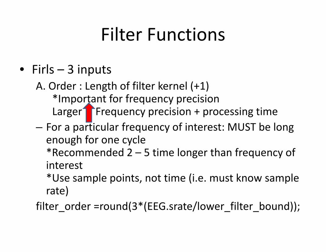
• Firls – 3 inputsA. Order : Length of filter kernel (+1)
*Important for frequency precisionLarger Frequency precision + processing time
– For a particular frequency of interest: MUST be long enough for one cycle*Recommended 2 – 5 time longer than frequency of interest*Use sample points, not time (i.e. must know sample rate)
filter_order =round(3*(EEG.srate/lower_filter_bound));

Filter Functions• Firls – 3 inputs
B. 6 numbers define shape of response1. Zero frequency
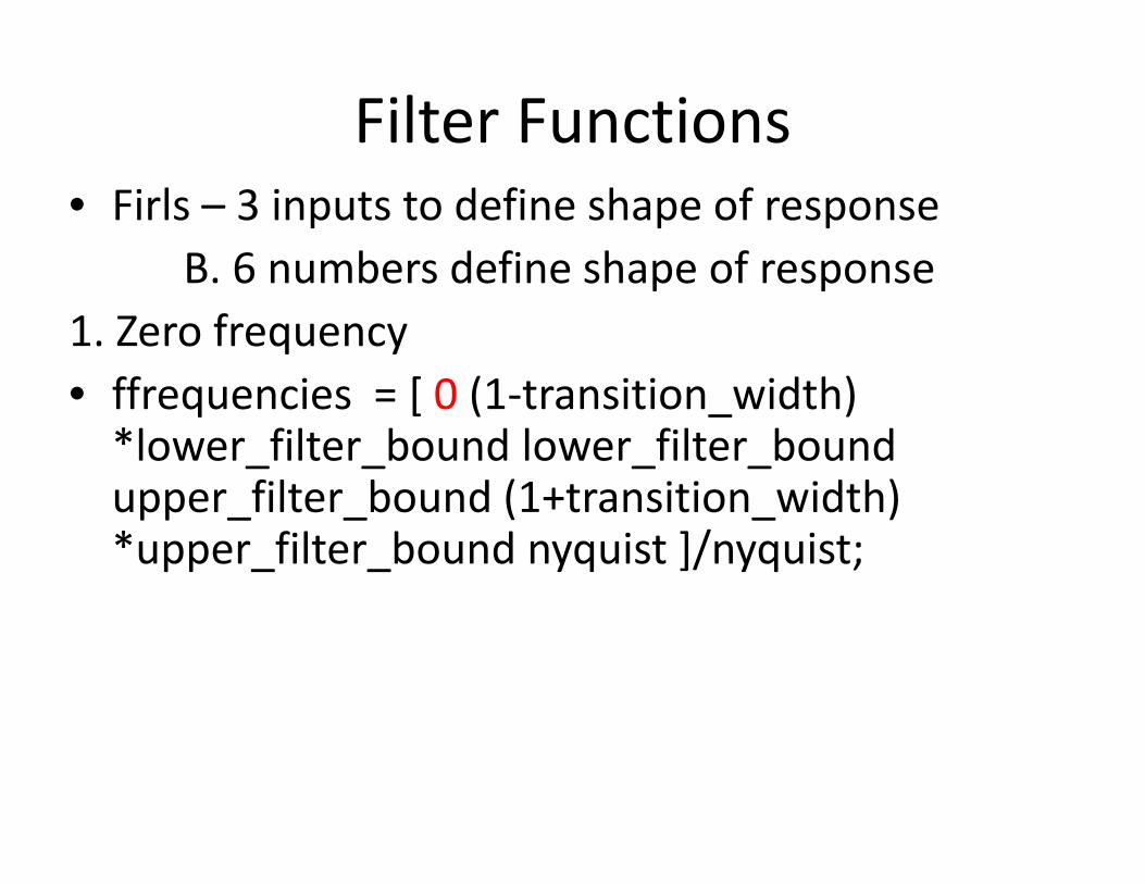
Filter Functions• Firls – 3 inputs to define shape of response
B. 6 numbers define shape of response 1. Zero frequency• ffrequencies = [ 0 (1‐transition_width) *lower_filter_bound lower_filter_boundupper_filter_bound (1+transition_width)*upper_filter_bound nyquist ]/nyquist;
Filter Functions• Firls – 3 inputs
B. 6 numbers define shape of response2. Frequency of start –lower transition zone

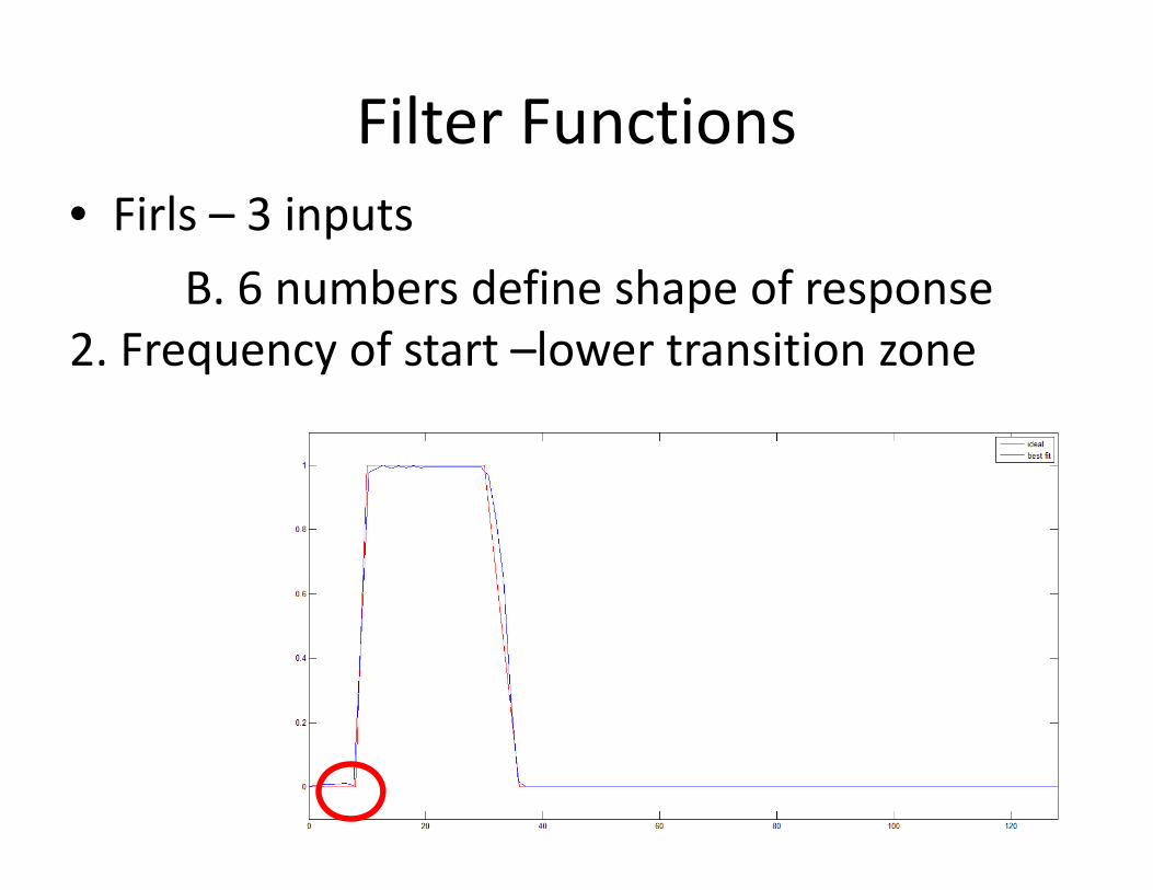
Filter Functions• Firls – 3 inputs
B. 6 numbers define shape of response 2. Frequency of start –lower transition zonetransition_width = 0.2;lower_filter_bound = 4; % Hz
ffrequencies = [ 0 (1‐transition_width) *lower_filter_bound lower_filter_boundupper_filter_bound (1+transition_width)*upper_filter_bound nyquist ]/nyquist;
Filter Functions• Firls – 3 inputs
B. 6 numbers define shape of response3. Lower bound of bandpass
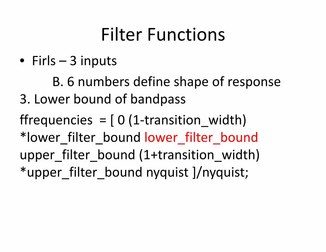
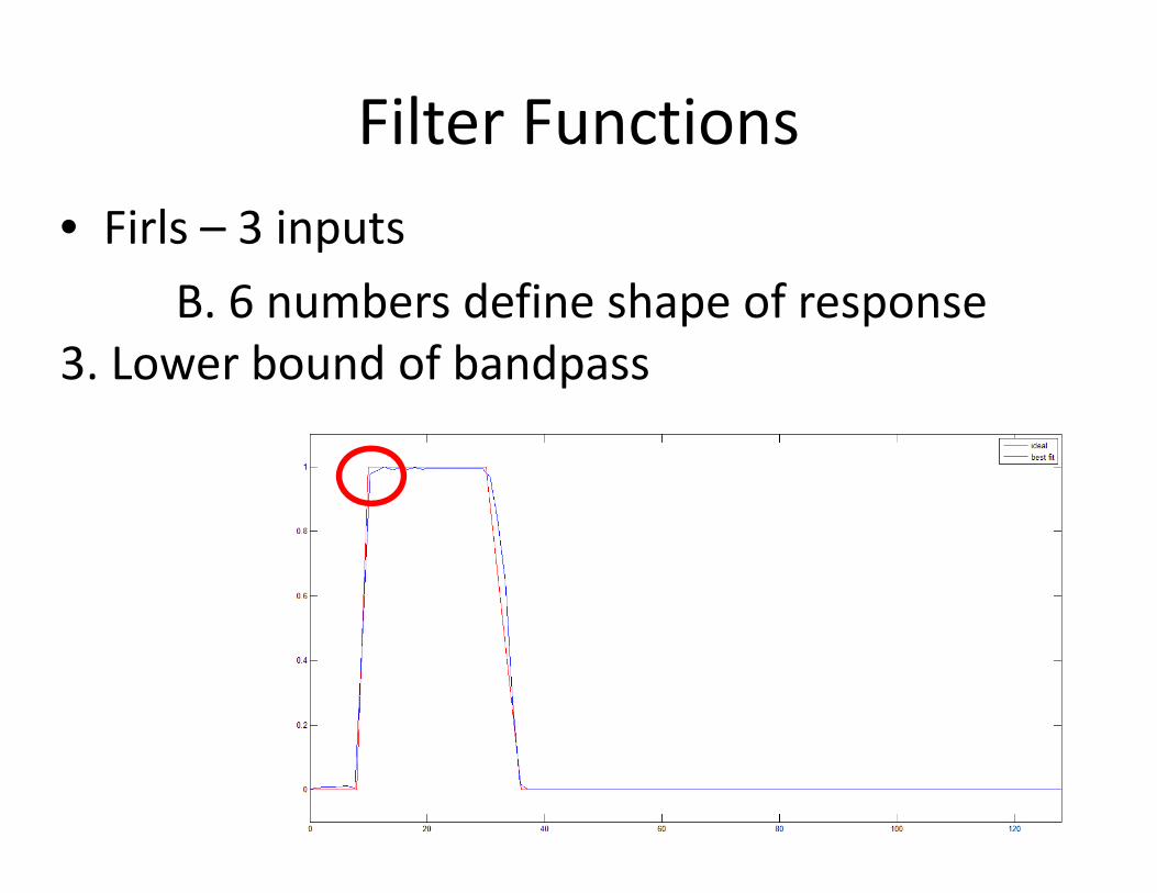
Filter Functions• Firls – 3 inputs
B. 6 numbers define shape of response 3. Lower bound of bandpassffrequencies = [ 0 (1‐transition_width) *lower_filter_bound lower_filter_boundupper_filter_bound (1+transition_width)*upper_filter_bound nyquist ]/nyquist;

Filter Functions
• Firls – 3 inputsB. 6 numbers define shape of response
Side note: Transition zones
Transition zones
Filter Functions
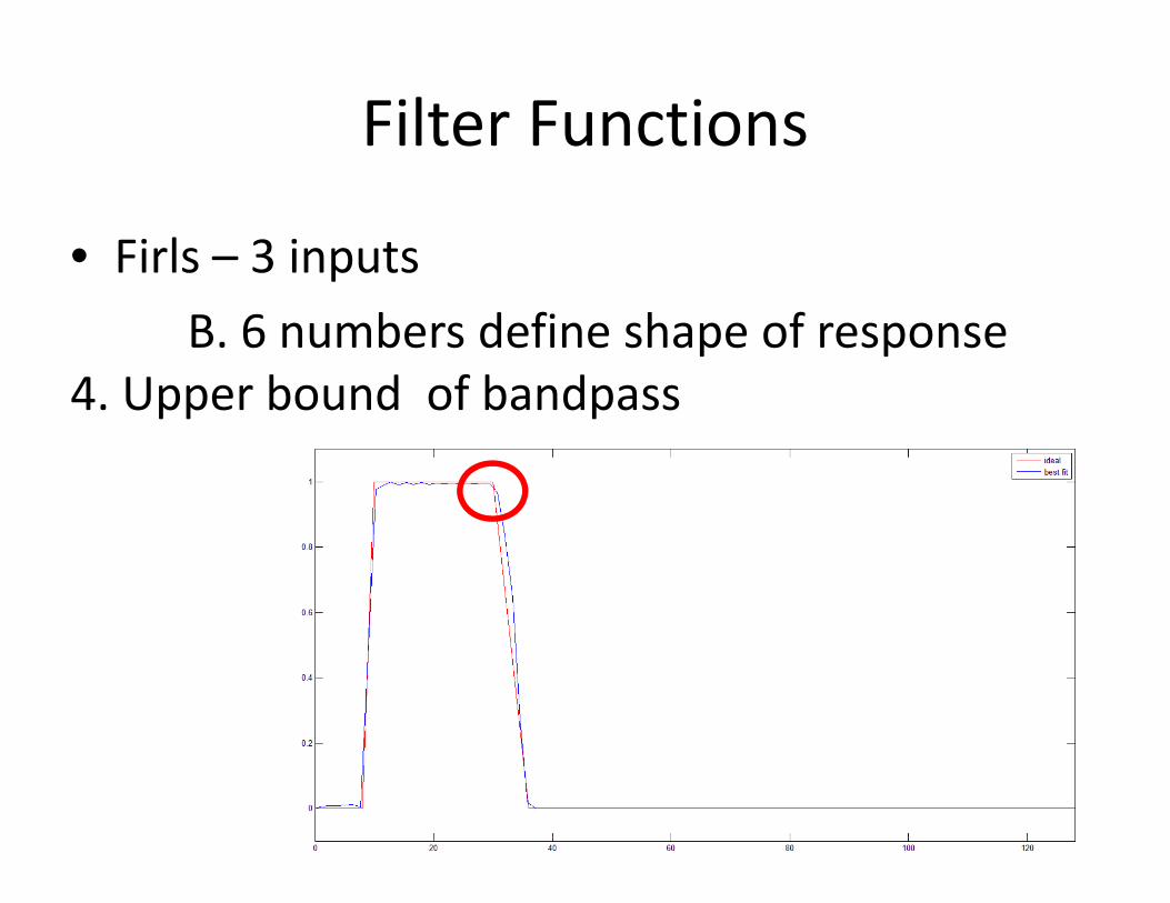
• Firls – 3 inputsB. 6 numbers define shape of response
4. Upper bound of bandpass
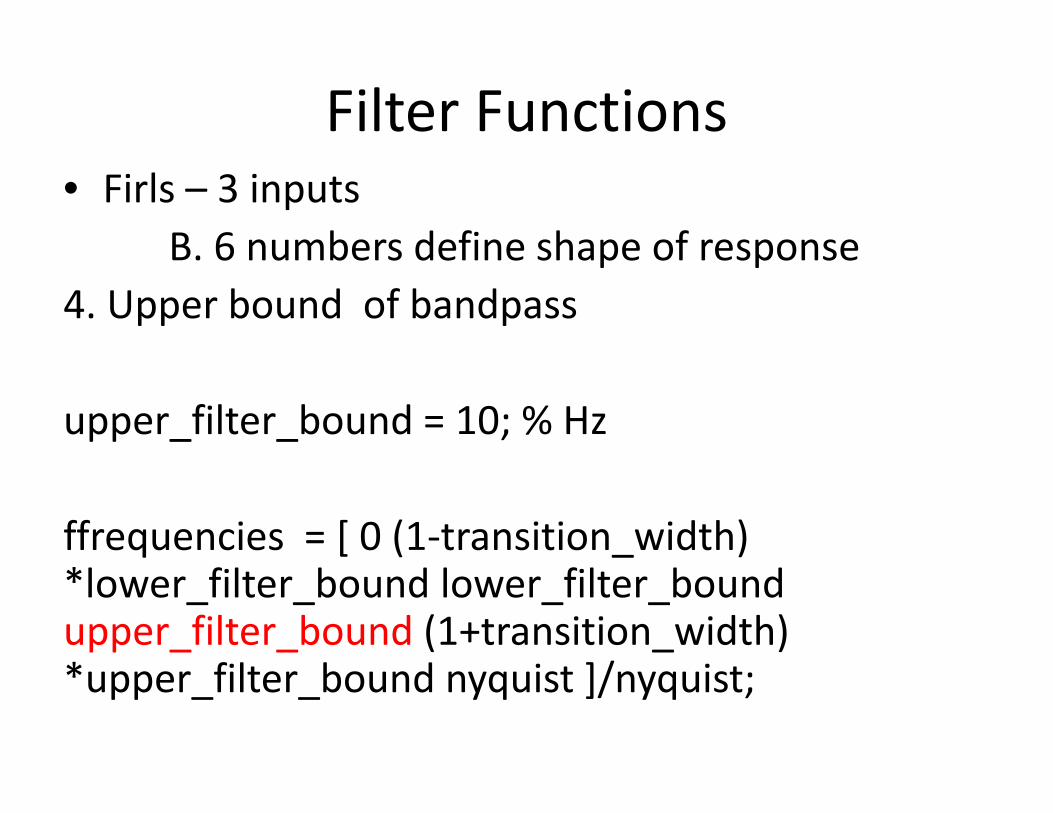
Filter Functions• Firls – 3 inputs
B. 6 numbers define shape of response 4. Upper bound of bandpass
upper_filter_bound = 10; % Hz
ffrequencies = [ 0 (1‐transition_width) *lower_filter_bound lower_filter_boundupper_filter_bound (1+transition_width)*upper_filter_bound nyquist ]/nyquist;
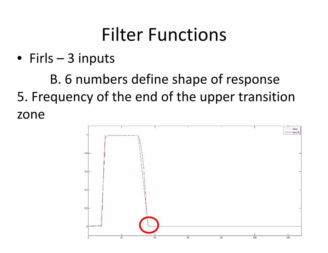
Filter Functions• Firls – 3 inputs
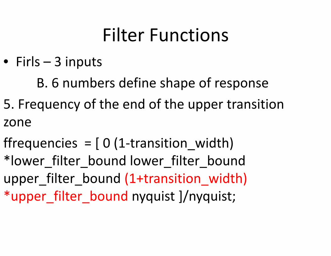
B. 6 numbers define shape of response5. Frequency of the end of the upper transitionzone
Filter Functions• Firls – 3 inputs
B. 6 numbers define shape of response 5. Frequency of the end of the upper transitionzone ffrequencies = [ 0 (1‐transition_width) *lower_filter_bound lower_filter_boundupper_filter_bound (1+transition_width)*upper_filter_bound nyquist ]/nyquist;
Filter Functions• Firls – 3 inputs
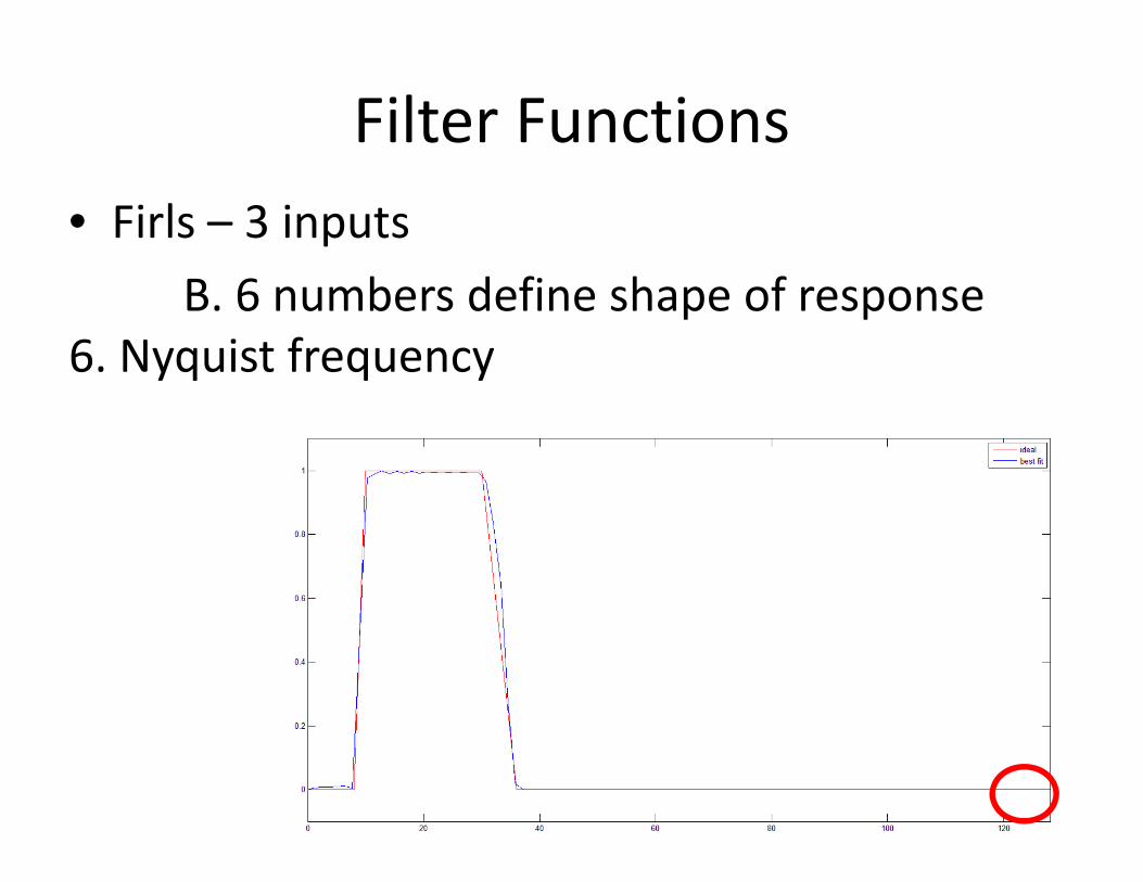
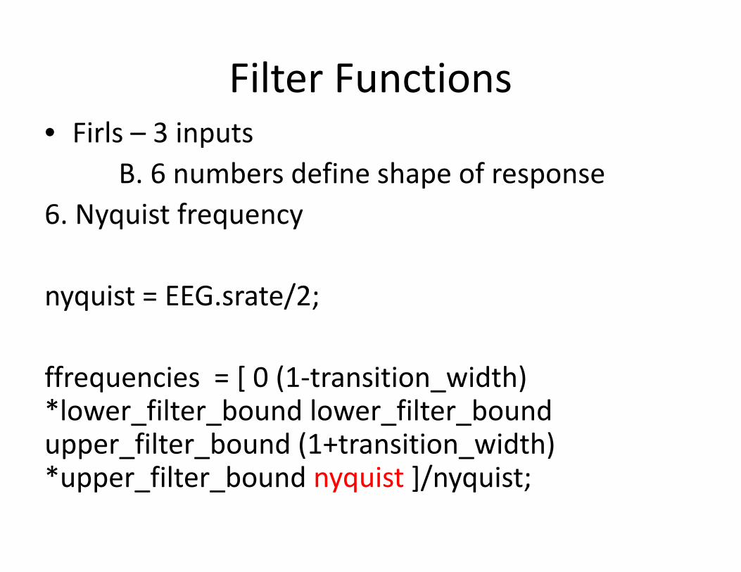
B. 6 numbers define shape of response6. Nyquist frequency
Filter Functions• Firls – 3 inputs
B. 6 numbers define shape of response 6. Nyquist frequency
nyquist = EEG.srate/2;
ffrequencies = [ 0 (1‐transition_width) *lower_filter_bound lower_filter_boundupper_filter_bound (1+transition_width)*upper_filter_bound nyquist ]/nyquist;

Filter Functions
• Firls – 3 inputsB. 6 numbers define shape of response‐ These numbers are scaled so that Nyquistfrequency is 1.‐Once frequencies are set in Hz we divide by the nyquist frequency
ffrequencies = [ 0 (1‐transition_width) *lower_filter_bound lower_filter_boundupper_filter_bound (1+transition_width)*upper_filter_bound nyquist ]/nyquist;

Filter Functions• Firls – 3 inputs
C. Ideal response amplitudeLength of ideal response should = 6 numbers define shape of response0s = attenuate . 1s = keep. Can use range 0‐1
[0 0 1 1 0 0]
Lower UpperFrequency bounds

Filter Functions
• Firls – 3 inputsC. Ideal response amplitude
Length of ideal response should = 6 numbers define shape of response
[0 0 1 1 0 0] DC Nyquist
Lower UpperFrequency bounds of transition zones

Frequency Width
• Controls Time Frequency trade offNarrow Width
Frequency PrecisionTemporal Precision
Wide WidthTemporal Precision Frequency Precision Time
Freq
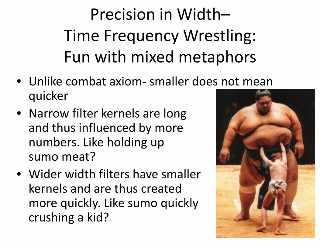
Precision in Width–Time Frequency Wrestling:Fun with mixed metaphors
• Unlike combat axiom‐ smaller does not mean quicker
• Narrow filter kernels are longand thus influenced by more numbers. Like holding up sumo meat?
• Wider width filters have smallerkernels and are thus createdmore quickly. Like sumo quicklycrushing a kid?
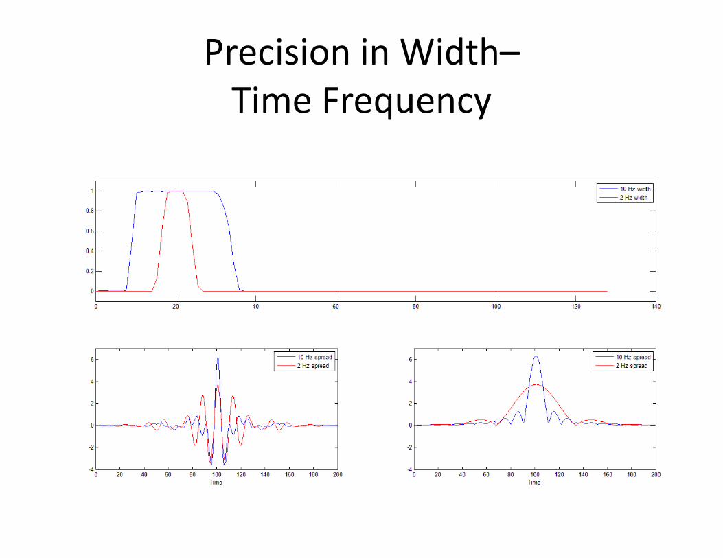
Precision in Width–Time Frequency
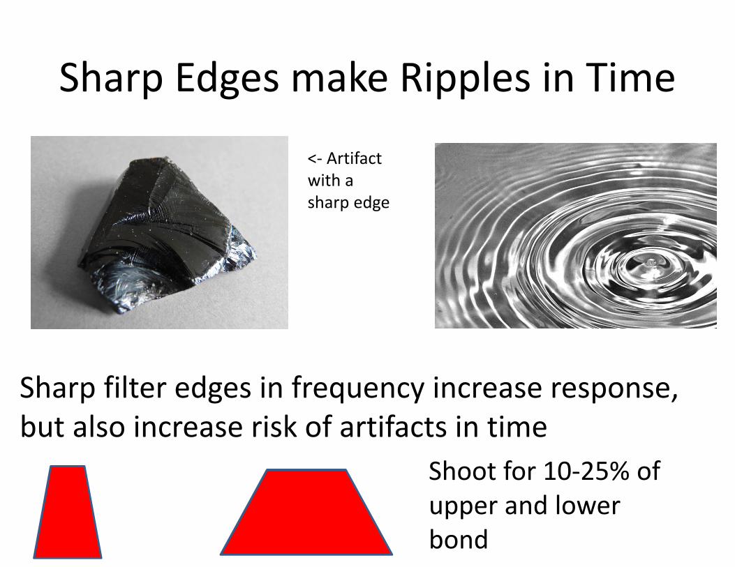
Sharp Edges make Ripples in Time
Sharp filter edges in frequency increase response, but also increase risk of artifacts in time
Shoot for 10‐25% of upper and lower bond
<‐ Artifact with a sharp edge
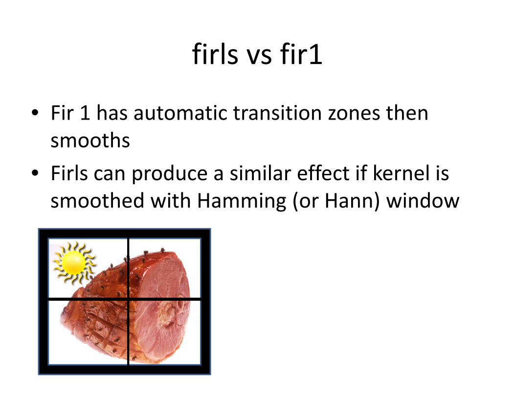
firls vs fir1
• Fir 1 has automatic transition zones then smooths
• Firls can produce a similar effect if kernel is smoothed with Hamming (or Hann) window

See the same… minus the ham
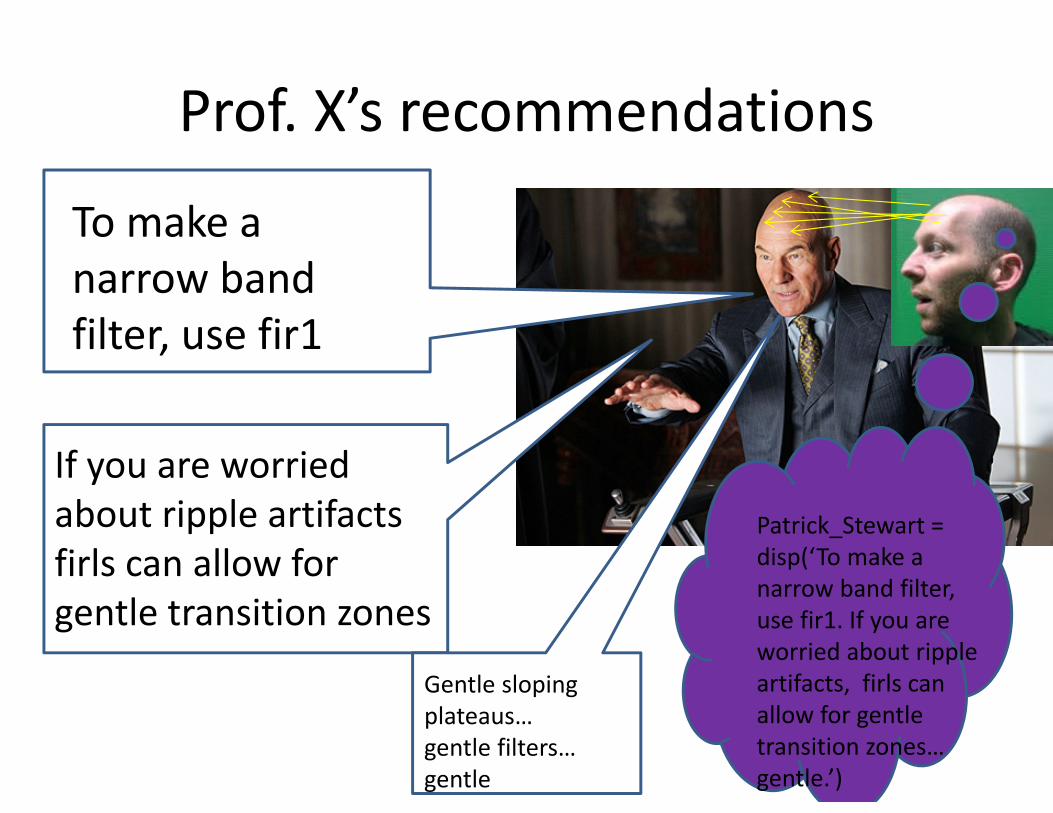
Prof. X’s recommendations
Patrick_Stewart = disp(‘To make a narrow band filter, use fir1. If you are worried about ripple artifacts, firls can allow for gentle transition zones… gentle.’)
To make a narrow band filter, use fir1
If you are worried about ripple artifacts firls can allow for gentle transition zones
Gentle sloping plateaus… gentle filters… gentle

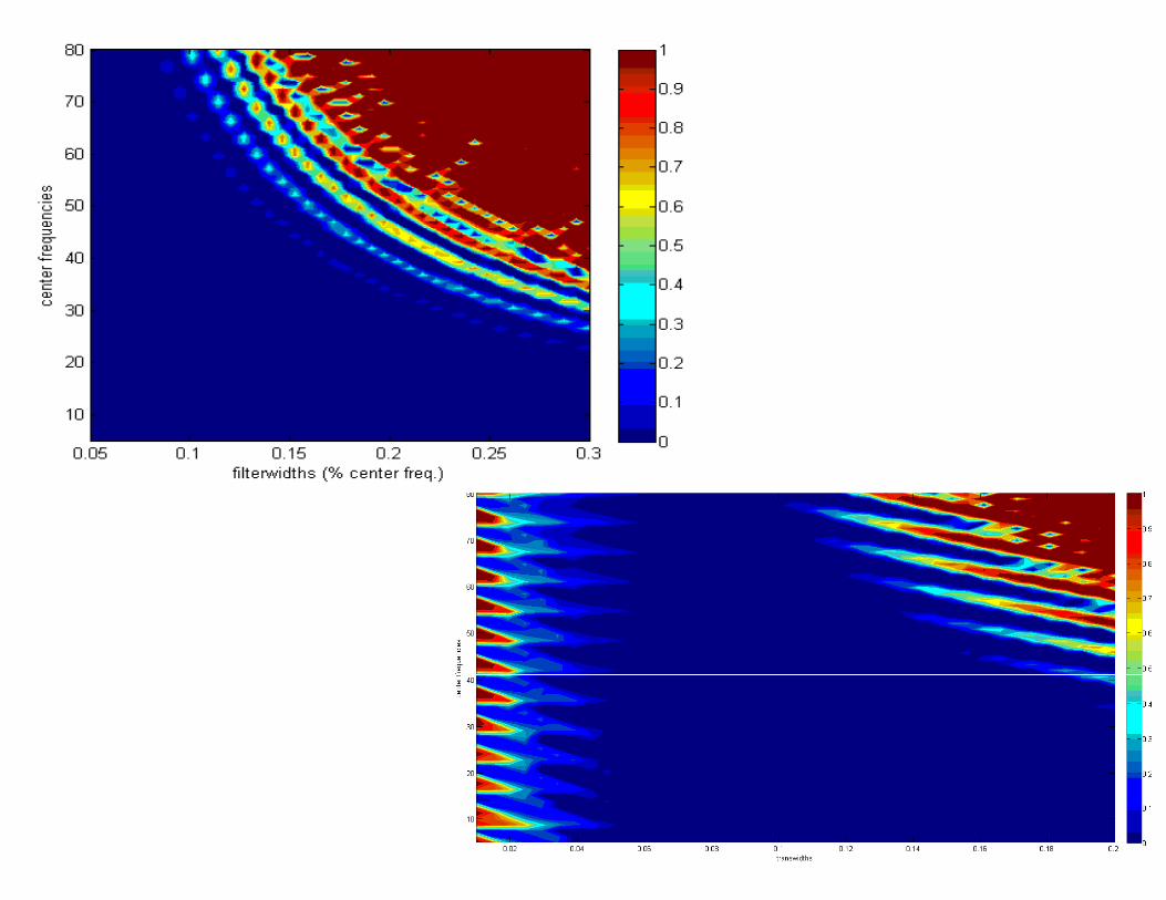
Check.Your.Filters:So Whatcha Want?
Goodness quantified!
Ideal forms:Similarity between actual filter and the ideal filter
Sum of squared errors
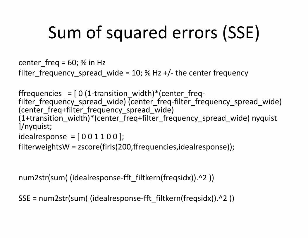
Sum of squared errors (SSE)center_freq = 60; % in Hzfilter_frequency_spread_wide = 10; % Hz +/‐ the center frequency
ffrequencies = [ 0 (1‐transition_width)*(center_freq‐filter_frequency_spread_wide) (center_freq‐filter_frequency_spread_wide) (center_freq+filter_frequency_spread_wide) (1+transition_width)*(center_freq+filter_frequency_spread_wide) nyquist]/nyquist;idealresponse = [ 0 0 1 1 0 0 ];filterweightsW = zscore(firls(200,ffrequencies,idealresponse));
num2str(sum( (idealresponse‐fft_filtkern(freqsidx)).^2 ))
SSE = num2str(sum( (idealresponse‐fft_filtkern(freqsidx)).^2 ))
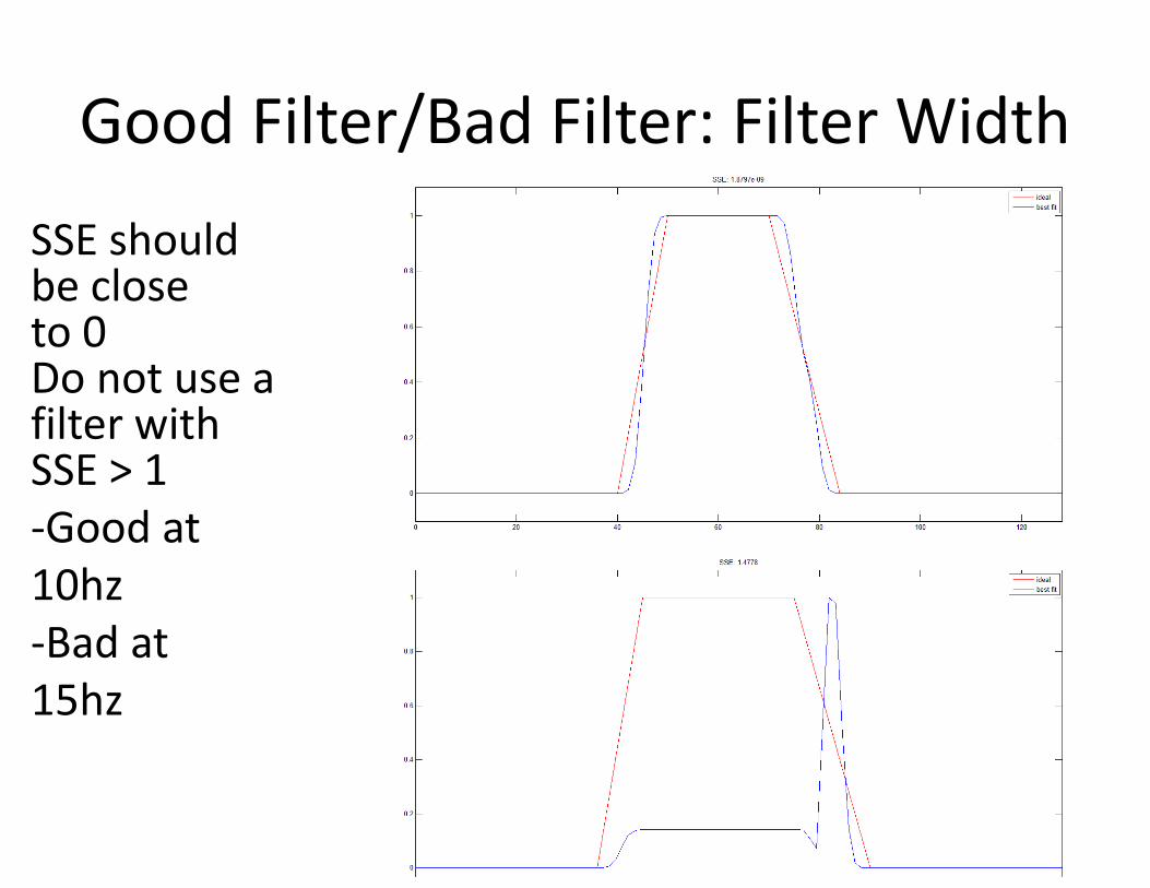
Good Filter/Bad Filter: Filter Width
SSE shouldbe closeto 0Do not use afilter withSSE > 1‐Good at10hz‐Bad at15hz

Application: filtfilt
• After creating the perfect kernel and testing it• Filtfilt used to applydata2filter = squeeze(double(EEG.data(47,:,1)));filterweights = firls(200,ffrequencies,idealresponse); % recomputewithout z‐scoringfilter_result = filtfilt(filterweights,1,data2filter);
Filter Kernel ‐‐Weight coefficient ‐‐ Data

Filtfilt compared to convolution

Phase Delay and Time Travel
• Causal filter : Filter is based on information from the past (back in time)
• Filter function: Causes a phase delay

Phase Delay and Time Travel
• Luckily we can filter back in time to correct the errors of the past!
• Forward_to_the‐past = 1‐(Back_to_the_Future)• Refiltering corrects the phase delay
I need a nuclear reaction to generate 1.21 JIGAwatts of electricity.
Damn it DOC, my mat‐telepathy demands GIGA! GIGAWATTS

You thought your puny mat‐telepathy powers could defeat me? With my Infinity Impulse Response Filtering death ray I will sow (relative) chaos, instability and non linear phase distortions across your signal! Bwahahaha
NOOOOO!5th order Butterworth
Hope for analytic signal… fading…must use Hilbert powers to… transform

Revenge of the Hilbert Transform
• Remember way back‐ before time traveling filters, sumo quick narrow filters, and (poor) comic book‐ish fight scenes?
• Analytic signal produced by adding phase quadrature (1/4)
• Created by rotating aspects of complexfrequency spectrum (from Fourier)
Concatenation powers activate!Hilbert transform!
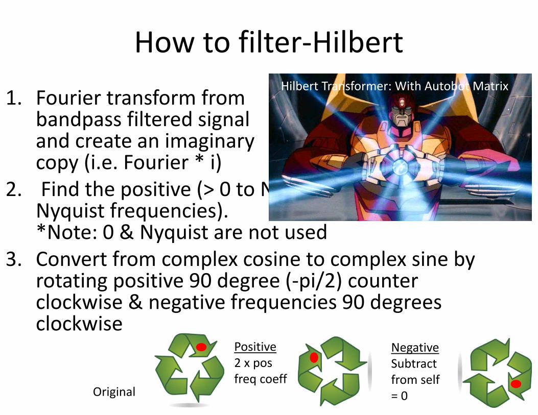
How to filter‐Hilbert
1. Fourier transform from bandpass filtered signal and create an imaginarycopy (i.e. Fourier * i)
2. Find the positive (> 0 to Nyquist) and negative (> Nyquist frequencies). *Note: 0 & Nyquist are not used
3. Convert from complex cosine to complex sine by rotating positive 90 degree (‐pi/2) counter clockwise & negative frequencies 90 degrees clockwise
Hilbert Transformer: With Autobot Matrix
Original
Positive 2 x posfreq coeff
NegativeSubtract from self = 0
How to Hilbert
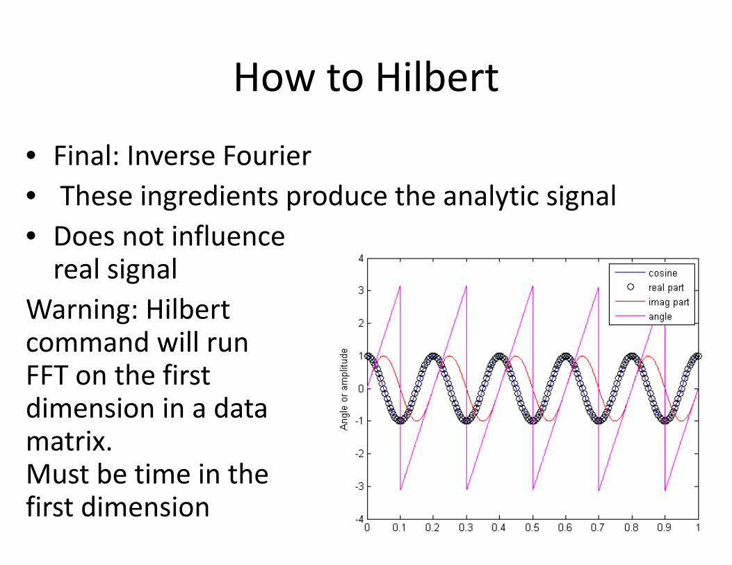
• Final: Inverse Fourier• These ingredients produce the analytic signal • Does not influencereal signal
Warning: Hilbert command will run FFT on the firstdimension in a datamatrix. Must be time in the first dimension

Double check your signal
• Plot phase angles!

Come my allies, we have earned goodnight’s sleep


