Bank Runs and the Diamond-Dybvig (1983)Model

ECON 43370: Financial Crises

Eric Sims

University of Notre Dame

Spring 2019

1 / 26

Bank Runs

I Bank runs, broadly construed, are a recurrent theme ineconomic history

I Financial crises are about runs on short term bank debt

I Situation in which short term liability holders “run” en masseto liquidate their savings in financial intermediaries, forcingintermediaries to engage in asset sales that could leave theminsolvent

I Why are runs so prevalent?

I Why do people hold short term bank debt (e.g. deposits) if itis nevertheless susceptible to runs?

I What type of policies can be used to prevent/reduce/mitigateruns?

2 / 26

Diamond-Dybvig (1983) Model

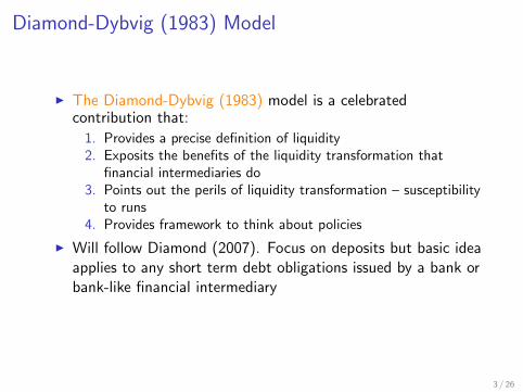
I The Diamond-Dybvig (1983) model is a celebratedcontribution that:

1. Provides a precise definition of liquidity2. Exposits the benefits of the liquidity transformation that

financial intermediaries do3. Points out the perils of liquidity transformation – susceptibility

to runs4. Provides framework to think about policies

I Will follow Diamond (2007). Focus on deposits but basic ideaapplies to any short term debt obligations issued by a bank orbank-like financial intermediary

3 / 26

Model BasicsI There are three periods, indexed by T : T = 0, T = 1, T = 2.

T = 0 is the “present” and T = 1, 2 measure the “future”I There are (many) households who are (ex-ante) identical and

are endowed with 1 in T = 0 and will need to consume ineither T = 1 or T = 2

I Idiosyncratic uncertainty: individual does not know (atT = 0) whether she will be type 1 (needs to consume inT = 1) or type 2 (can wait to consume until T = 2). Typerevealed in T = 1

I But there is no aggregate uncertainty: a fixed fraction,t ∈ [0, 1], of households will be type 1 and a fixed fraction1− t type 2

I There are two assets:1. Storage (cash): save 1 in T = 0, have 1 available to consume

in either T = 1 or T = 22. Illiquid investment opportunity: save 1 in T = 0, can get r1

(gross) if liquidated (sold) in T = 1, and r2 ≥ r1 if liquidatedin T = 2

4 / 26

Preferences

I An individual household has utility:

U(c) = 1− 1

c

I Its expected utility is simply the probability-weighted sum ofutility flows depending on which type it ends up being:

E[U ] = tU(c1) + (1− t)U(c2)

I Where c1 and c2 are consumption at each date depending ontype

I Consumption allocations: c1 = c2 = 1 if storage, c1 = r1 andc2 = r2 if invest

5 / 26

Numerical Example

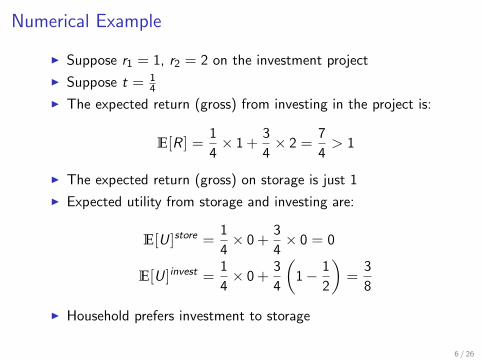
I Suppose r1 = 1, r2 = 2 on the investment project

I Suppose t = 14

I The expected return (gross) from investing in the project is:

E[R ] =1

4× 1 +

3

4× 2 =

7

4> 1

I The expected return (gross) on storage is just 1

I Expected utility from storage and investing are:

E[U ]store =1

4× 0 +

3

4× 0 = 0

E[U ]invest =1

4× 0 +

3

4

(1− 1

2

)=

3

8

I Household prefers investment to storage

6 / 26

Liquidity

I We can think about the liquidity of an asset as the discountone has to pay for “early” liquidation

l =r1r2

I Since r2 ≥ r1 (by assumption), l ≤ 1

I The further l is from 1, the less liquid is the asset

I Cash is perfectly liquid, l = 1 – you get 1 regardless of whenyou access it

I Investment is less liquid, l = 12

I Though in this example you still prefer to hold the less liquidinvestment

7 / 26

Alternative Example with Less Liquid Investment

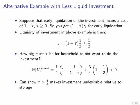
I Suppose that early liquidation of the investment incurs a costof 1− τ, τ ≥ 0. So you get (1− τ)r1 for early liquidation

I Liquidity of investment in above example is then:

l = (1− τ)1

2≤ 1

2

I How big must τ be for household to not want to do theinvestment?

E[U ]invest =1

4

(1− 1

1− τ

)+

3

4

(1− 1

2

)< 0

I Can show τ > 35 makes investment undesirable relative to

storage

8 / 26

Example with τ = 23

I Expected utility from storage versus investment:

E[U ]store = 0

E[U ]invest =1

4×(

1− 113

)+

3

4×(

1− 1

2

)= −1

8

I Now household prefers storage to investment!

I Even though expected (gross) return to investment is higher:

E[R ]store = 1

E[R ]invest =1

4× 1

3+

3

4× 2 =

19

12> 1

I If project is sufficiently illiquid and/or household is sufficientlyrisk averse (i.e. u′′(C ) < 0), then household may not want todirectly invest in positive net return projects

9 / 26

A Bank and Liquidity Transformation

I A mutual bank (no equity, not trying to make profit for itself)can potentially step in and make households better offregardless of whether households would directly fund theinvestment project or not

I How? In essence by exploiting law of large numbers andengaging in what amounts to provision of insurance

I An individual household is uncertain about when she will needto consume: this gives rise to a preference for liquidity

I But in the aggregate there is no uncertainty – exactly thefraction t of households will be type 1 and 1− t will be type 2

I Bank can pool resources from many households exploiting thislack of aggregate uncertainty and offer households an assetthat is more liquid than the investment project that thehousehold prefers to both direct investment and storage

10 / 26

Deposits

I Same setup as earlier: r1 = 1, r2 = 2, t = 14 , and τ = 0

I Suppose bank offers household an asset with the followingpayout structure: rd1 = 1.28 and rd2 = 1.813 (gross returndepending on date of liquidation)

I This is more liquid than the investment opportunity:1.281.813 = 0.706 > 1

2I How does this work? Suppose there are 100 households and

exactly 25 will need to withdraw in period T = 1I Bank takes 100 in T = 0 and puts it into 100 units of the

investment (assume r1 and r2 independent of amountinvested)

I Will need to liquidate 25× 1.28 = 32 units of the investmentto raise necessary funds in T = 1, leaving 68 invested

I These 68 will generate 136 in income in T = 2, which can bedistributed to remaining 75 deposit holders forr2 =

13675 = 1.813

11 / 26

Which Does Household Prefer?

I An individual household has three options: storage (expectedgross return 1), deposits (expected gross return 1.68), ordirect investment (expected gross return 2)

I Which does it prefer? Expected utilities:

E[U ]store = 0

E[U ]invest =3

8

E[U ]deposit =1

4×(

1− 1

1.28

)+

3

4×(

1− 1

1.813

)= 0.391 >

3

8

I A household’s best option is deposits!

I Household willing to tolerate a lower expected return ondeposits because of higher liquidity of deposits relative todirect investment

I Can make this even starker if τ > 0

12 / 26

Consumption Smoothing and Preference for Liquidity

I We have assumed household is risk averse and uncertainabout when it will need to consume

I Given risk aversion (U ′′(c) < 0), household has incentive tosmooth consumption across states (i.e. type 1 or type 2)

I If it directly invests in project, marginal utility (U ′(C )) is highif type 1 (gets comparatively low return) and low if type 2(gets comparatively high return)

I Would like to potentially reallocate some consumption fromtype 2 state (low marginal utility) to type 1 state (highermarginal utility) – i.e. would like something more liquid

I Would even be willing to sacrifice some expected return to getthis

13 / 26

Liquidity Transformation is Like Insurance

I The bank is engaging in liquidity transformationI It is creating an asset (deposit, which is a liability to bank but

asset to household) that is more liquid than the underlyingasset it is investing in

I In so doing, it can make households better off

I This is essentially functioning just like insurance – give upsome consumption in “good states” (low marginal utility, type2) by paying a “premium” to get some extra consumption in“bad states” (high marginal utility, type 1)

I The bank can offer this, just like an insurance company, byplaying law of large numbers

I With aggregate uncertainty things would be more complicatedbut the basic gist would be the same

14 / 26

Nash Equilibrium

I With many households and a mutual bank, the outcomedescribed above is a Nash Equilibrium

I Everyone is behaving optimally given beliefs about how othersare going to play ⇒ no incentive to deviate

I If I wake up in T = 1 and am revealed type 2, I do worse bywithdrawing in T = 1 (rd1 = 1.28) than by waiting untilT = 2 (rd2 = 1.813)

I Provided I think other type 2s are going to wait, it’s optimal towait, all type 2s will do this, and then beliefs are self-fulfilling

I When would it make sense to withdraw in T = 1 even if Idon’t have to?

I Only if I think I will get back less than 1.28 in T = 2I I think (enough) other type 2’s are going to withdraw “early”I I’m worried the bank’s investments are going to go bad

15 / 26

Good vs. Bad Equilibrium

I Let’s not worry about the “bank’s investments are going to gobad” reason for withdrawing early – this requires someaggregate uncertainty we don’t want to worry about, thoughimportant in the real world

I Let’s focus on multiplicity of equilibria with no aggregateuncertainty

I Good equilibrium: what we just described

I Bad equilibrium: type 2’s withdraw early in T = 1 becausethey expect other type 2’s to withdraw early as well, which willcause the bank to fail and make everyone (weakly) worse off

16 / 26

Early Withdrawals

I Let f denote the fraction of depositors who withdraw inT = 1; f ≥ t

I In our example, withdrawals in T = 1 are due rd1 = 1.28.With 100 deposits, bank must liquidate 128× f of theinvestment to meet this withdrawal demand

I This leaves (100− 128f ) invested, which itself earns a returnof 2 which can be distributed to the remaining (1− f )100depositor holds in T = 2:

rd2 =2(100− 128f )

(1− f )100

I When f = t = 1/4, then we get rd2 = 1.813

I But if f > t (some type 2s withdraw), then rd2 < 1.813.

17 / 26

Expectations

I Let f̂ be the expectation of each household about what f willbe (i.e. the fraction who will withdraw in T = 1)

I Suppose f̂ = 12 – you think half the population is going to

withdraw, or 1/3 of the type 2’s withdraw earlier than needed

I Is this expectation self-fulfilling? If f̂ = 12 , then:

r̂d2 =2(100− 128f̂ )

(1− f̂ )100= 1.44

I This is less than what was promised (rd2 = 1.813), butnevertheless better than what you get for withdrawing today

I So it cannot be optimal for type 2s to withdraw early giventhis forecast (they’re better off waiting), so f̂ = 1

2 is notself-fulfilling, because even if it is believed by everyone, onlyf = t = 1

4 will withdraw, so not an equilibrium

I So f̂ = f = t = 14 is a Nash Equilibrium

18 / 26

The Bad Equilibrium

I Suppose instead that f̂ = 34 . Then people will believe they

will get:

r̂d2 =2(100− 128f̂ )

(1− f̂ )100= 0.32

I This is (significantly) worse than rd1 – given this belief, best to“get out now”

I But then f̂ = 34 is not self-fulfilling: if that’s what everyone

believes, then everyone should withdraw

I So f̂ = f = 1 is another Nash Equilibrium

I Note it is completely rational (from the perspective of a type2 household) to withdraw in T = 1 given this belief

19 / 26

The Bad Equilibrium Continued

I If everyone withdraws, the bank will fail

I It can at most come up with $100 in T = 1, so it can’t evenmeet the promised rd1

I Typically there is a “first come, first served” aspect – the first78 people to line up (100/1.28 ≈ 78) are “made whole” andget rd1 = 1.28, but the last 22 get nothing

I This increases incentive to withdraw and withdraw early – youlose out by not being first in line

I Two equilibria: good (no run) and bad (run)

20 / 26

Equilibrium Selection

I How do we know which equilibrium will be “played”?

I We don’t

I There will exist a cutoff f̄ above which any f̂ → 1 (run) andbelow which f̂ → t (no run)

I In this example, f̄ = 0.5625

I As long as this is pretty far above t, will spend most of timein “good” equilibrium

I Would take a big event that is widely observed to move beliefsenough to switch to the run equilibrium

I Sometimes referred to as sunspots: big and easily observed byeveryone

21 / 26

Dealing with Runs

I Financial intermediation (i.e. “borrow short, lend long”) isstructurally subject to runs because of liquidity transformation

I Given that runs can occur, what kind of policies can beinstituted to deal with runs once they start?

I Key point: a policy which effectively deals with runs oughtnot to really need to be used in practice

I Knowledge of an effective policy once a run has starteddecreases the likelihood of a run happening in the first place

I e.g. if I know my deposits are safe no matter how many type2s withdraw early, I have no reason to withdraw early, and westay in the “good” equilibrium

22 / 26

Suspension of ConvertibilityI Prior to a well-organized central bank in the US, private banks

dealt with (recurrent) runs internally via clearinghouses(consortiums of banks in a location, e.g. New York)

I Principal means by which this was done was suspension ofconvertibility

I Simply refuse (temporarily) to honor demands for conversionof bank debt (e.g. deposits) into cash

I Banks did this together (effectively banding together as onelarge bank rather than many small banks for the duration ofthe crisis)

I Would lift suspension when panic was overI In practice was economically costly and didn’t stop runs from

happening, but was pretty effective at preventing liquiditycrises to force banks into insolvency

I Key difficulty: some people really do need their funds at shortnotice. How do you decide how much conversion to do beforesuspending? How do you make sure the cash gets into theappropriate hands?

23 / 26

Lender of Last Resort

I Federal Reserve was in large part brought into existence toattempt to more efficiently deal with the crises andsubsequent suspensions that had plagued US banking formuch of the 19th century

I Idea: central bank can create all the reserves it wants to

I If banks run out of cash to meet withdrawal demands, couldinstead go to the central bank to get requisite cash (thediscount window) – Bagehot’s rule

I People thought this would put an end to crisesI It didn’t (US Great Depression) for a variety of reasons:

1. Stigma: banks didn’t want to borrow from Fed for fear ofexposing themselves as weak

2. Fed itself didn’t understand its role and its powers (Friedmanand Schwartz)

24 / 26

Deposit Insurance

I In response to bank failures of early 1930s, Federal DepositInsurance Corporation (FDIC) was established in 1933

I Promised full value of deposits at member institutions up to acertain limiting value (originally $2,500, now $250,000) in theevent that the bank failed

I Who pays for this insurance? Banks pay a (small) fee to bemembers (like an insurance premium)

I In practice this has more or less eliminated traditional bankingpanics – people know deposits are safe, so no reason to run,and we stay in the good equilibrium

25 / 26

2007-2009

I If we had deposit insurance and we had the Fed, why wasthere a run in 2007-2009?

I The banking system changed

I New kinds of short term bank debt were introduced and roseto prominence

I No insurance on these new types of debt, and was unclearextent to which the Fed could or would serve as lender of lastresort to financial intermediaries that were not formally banks(deposit-taking institutions)

26 / 26