53
Working Paper/Document de travail 2014-7 Banks’ Financial Distress, Lending Supply and Consumption Expenditure by H. Evren Damar, Reint Gropp and Adi Mordel

Working Paper/Document de travail 2014-7
Banks’ Financial Distress, Lending Supply and Consumption Expenditure
by H. Evren Damar, Reint Gropp and Adi Mordel
2
Bank of Canada Working Paper 2014-7
February 2014
Banks’ Financial Distress, Lending Supply and Consumption Expenditure
by
H. Evren Damar,1 Reint Gropp2 and Adi Mordel1
1Financial Stability Department Bank of Canada
Ottawa, Ontario, Canada K1A 0G9 [email protected] [email protected]
2Goethe University Frankfurt, CFS and ZEW
Bank of Canada working papers are theoretical or empirical works-in-progress on subjects in economics and finance. The views expressed in this paper are those of the authors.
No responsibility for them should be attributed to the Bank of Canada, the Eurosystem or the European Central Bank.
ISSN 1701-9397 © 2014 Bank of Canada

ii
Acknowledgements
We would like to thank Jason Allen, Michael Ehrmann, Martin Goetz, Kim Huynh, John Krainer, Lorenz Kueng, Oren Levintal, Jim MacGee, Leonard Nakamura, Deyan Radev, Nicolas Serrano-Velarde, Jim Stock, Francesco Trebbi, and conference/seminar participants at the Joint Central Bank Conference at the Federal Reserve Bank of Cleveland, Frankfurt/Mannheim Macro Workshop, CAREFIN/Bocconi Conference on Financing the Recovery After the Crisis, 11th International Industrial Organization Conference, IBEFA 2012 Summer Meetings, Goethe University Frankfurt, the European Central Bank, the Federal Reserve Bank of San Francisco, the Bank of Israel and the Bank of Canada for valuable comments at various stages of this paper. The paper was written while Gropp was a Duisenberg research fellow at the European Central Bank and the hospitality of the ECB is gratefully acknowledged.

iii
Abstract
The paper employs a unique identification strategy that links survey data on household consumption expenditure to bank-level data in order to estimate the effects of bank financial distress on consumer credit and consumption expenditures. Specifically, we show that households whose banks were more exposed to funding shocks report significantly lower levels of non-mortgage liabilities compared to a matched sample of households. The reduced access to credit, however, does not result in lower levels of consumption. Instead, we show that households compensate by drawing down liquid assets. Only households without the ability to draw on liquid assets reduce consumption. The results are consistent with consumption smoothing in the face of a temporary adverse lending supply shock. The results contrast with recent evidence on the real effects of finance on firms’ investment, where even temporary adverse credit supply shocks are associated with significant real effects.
JEL classification: E21, E44, G21, G01 Bank classification: Financial institutions; Credit and credit aggregates; Domestic demand and components
Résumé
Les auteurs font appel à une stratégie d’identification unique qui établit un lien entre des données d’enquête sur les dépenses de consommation des ménages et des données concernant les institutions financières, afin d’estimer l’incidence des difficultés financières des banques sur le crédit à la consommation et les dépenses de consommation. Plus précisément, ils montrent que les ménages dont l’institution a été davantage exposée à des chocs de financement font état de niveaux d’engagements non hypothécaires beaucoup moins élevés que les ménages d’un échantillon apparié. Les auteurs constatent néanmoins que le resserrement de l’accès au crédit n’entraîne pas de diminution de la consommation, les ménages compensant la baisse en puisant dans leurs avoirs liquides; les seuls qui réduisent leur consommation sont ceux qui n’ont pas la possibilité d’utiliser de tels avoirs. Ces résultats concordent avec le lissage observé lors d’un choc négatif temporaire de l’offre de crédit. Ils s’opposent toutefois aux conclusions d’études récentes sur les effets réels d’une crise de financement sur les investissements des entreprises, qui indiquent que même des chocs négatifs temporaires de l’offre de crédit ont des effets réels considérables à cet égard.
Classification JEL : E21, E44, G21, G01 Classification de la Banque : Institutions financières; Crédit et agrégats du crédit; Demande intérieure et composantes

1 Introduction
This paper studies the effects of bank financial distress on household consumption. If financial
distress in banking adversely affects household consumption, due to, for instance, exacerbating
household credit constraints, this may have first-order macroeconomic consequences and would
exacerbate the real effects of banking distress. To our knowledge, this is the first paper that
attempts to identify the effect of bank distress on consumption.
Using Canadian household data before and during the financial crisis, we document a
statistically and economically significant reduction in the non-mortgage credit supply of dis-
tressed banks (that is, banks that were unable to obtain short-term funding from the United
States)1 to households - on the order of 8.1 billion Canadian dollars (a 2.2 per cent decline).
However, we also show that a temporary short-run contraction in credit supply to households
has only a negligible effect on consumption. Most households that are faced with an inability
to borrow do not reduce consumption expenditures, but rather draw down liquid assets to
maintain a smooth consumption stream. We show a reduction in consumption only for house-
holds that do not have sufficient liquid assets to compensate for the decline in access to credit.
Overall, the results are consistent with the permanent income hypothesis and consumption
smoothing, and suggest that short-run contractions in credit supply to households may only
have mild effects on consumption expenditure.
Aggregate Canadian data suggest that there was a noticeable dip in credit to households,
in consumption and, even more substantially, in durable consumption in 2008/2009 relative
to 2007, with a subsequent (weak) recovery in 2010 (Figure 1). This is despite the fact that
Canadian banks were only affected by the U.S. financial crisis inasmuch as they depended on
1As discussed in more detail below, we define “distress” only as the inability to obtain short-term fundingfrom the United States, which might cause a reduction in the amount of credit supplied by banks. We do notconsider more severe forms of distress such as insolvency or failure, which often require a bailout, given thatthere were no such instances in Canada during the recent financial crisis.

short-term finance in the U.S. money market. Attempting to distinguish how much of this
dip is due to households reducing their demand for consumption in the face of the financial
crisis2 versus banks reducing the loan supply is the challenge in the identification strategy we
face in this paper.
The data we use offer three distinct advantages in meeting this challenge. First, they
provide detailed information on a large set of Canadian households, not only for assets and
liabilities, but also for consumption expenditures. Second, the data establish a clean link
between the household and its main bank, which in turn can be linked to the bank’s balance
sheet. Third, we have access to confidential bank-level data on exposures to the U.S. money
market, which we assume is exogenous to household behaviour. We use this information to
distinguish banks with high exposure to the United States (referred to as “exposed banks”)
from those with low or no exposure (referred to as “unexposed banks”).
The paper links the literature on consumption smoothing with that on the real effects of
finance. Adverse selection models of credit (e.g., Stiglitz and Weiss (1981)) would suggest
that it may be optimal to cut off some households from credit entirely, rather than charge
them higher interest rates to compensate for higher risk. In the presence of such frictions,
changes in lending supply may affect household expenditures. At the same time, the standard
life cycle/permanent income model predicts that temporary changes in access to credit have
no effect on expenditure patterns.
Several authors have investigated these questions using variation from quasi-natural ex-
periments. For example, Agarwal, Liu and Souleles (2007) study tax refunds and show that
consumers first pay down debt and then increase spending. Gross and Souleles (2002) inves-
tigate an exogenous change in the credit limit for credit cards and find that households tend
2The so-called “CNN effect”: Canadians, even though they were not directly affected by the crisis, mayhave reduced or postponed demand for large consumption items simply in the face of reporting from theUnited States.
2

to spend more in response to this change. Alessie, Hochguertel and Weber (2005) use the
introduction of a usury law that limits interest rate charges on consumer loans and document
a positive effect on the demand for credit. Leth-Petersen (2010) shows that credit-constrained
households increased consumption in response to a credit market reform in Denmark that
gave households access to housing equity as collateral for consumption loans. Most recently,
Abdallah and Lastrapes (2012) use a constitutional amendment in Texas that relaxed re-
strictions on home equity lending to identify the effect of credit constraints on consumption
expenditure. They find significant positive effects on consumption, suggesting the presence of
credit constraints. Finally, Mian and Sufi (2010) show that households with high leverage as
of 2006 exhibited a sharp relative decline in durable consumption starting in the third quarter
of 2006 and continuing throughout the financial crisis of 2008/2009. However, they do not
attempt to distinguish demand from credit supply effects.
Our findings also contribute to the literature on the impact of income shocks on consumer
expenditure. Although we examine the effects of a reduction in the supply of credit, as opposed
to lower income, both of these shocks tighten the current constraints faced by households and
are likely to have similar effects on spending. Existing studies on the response of consumption
to income changes, however, have mostly focused on permanent shocks. The literature (for
recent surveys see Jappelli and Pistaferri (2010) and Meghir and Pistaferri (2011)) would
suggest that permanent and temporary changes in credit supply to households would have
quite different effects on consumption expenditure. In particular, as long as households expect
credit conditions to improve in the future, they may offset a decline in credit supply through
drawing down assets in order to maintain consumption.
It should also be noted that our findings are based on households simultaneously carrying
debt and holding liquid assets. Specifically, for the negative credit supply to have an impact
on household spending during the crisis period, one expects households to be using debt
for spending (or investment) even during the pre-crisis period. On the other hand, most
3

households use liquid assets to smooth consumption during the crisis, so the households in
our sample are in fact keeping liquid assets and carrying debt at the same time. Although
puzzling upon first glance, this behavior has been frequently observed in the literature (for
example, by Gross and Souleles (2002)). Among the few proposed explanations, Telyukova and
Wright (2008) argue that households simultaneously carry debt and hold liquid assets since
some unexpected expenses cannot be paid for by credit. Therefore, holding liquid assets, even
at the expense of carrying some debt, can be loosely considered as a type of precautionary
savings. We do not take a stance on why the households in our sample might be displaying
this behavior, since the precise mechanism is not directly relevant for our results.
Our results contrast with recent findings on the effect of adverse lending supply shocks on
investment.3 Temporary contractions of lending supply tend to affect investment spending
and employment by firms. For example, Campello, Graham and Harvey (2010) show that
credit-constrained firms planned deeper cuts in spending and employment. They also find
that the inability to borrow externally caused many firms to circumvent attractive investment
opportunities. Dell’Ariccia, Detragiache and Rajan (2008) find evidence that business sectors
more dependent on external finance perform relatively worse during banking crises. Puri,
Rocholl and Steffen (2011), using an empirical approach similar to ours, show that banks with
a larger exposure to the recent financial crisis reduced credit to firms by a larger amount.4
3Cohen-Cole et al. (2008) show that credit supply declined during the crisis. However, it did not decline byas much for banks with a larger reliance on retail deposits (Ivashina and Scharfstein (2010); Gozzi and Goetz(2010)). Furthermore, banks that incurred larger subprime losses charged their corporate borrowers higherloan rates (Santos (2011)).
4Earlier contributions to the literature on the effect of lending supply shocks include Peek and Rosengren(1997, 2000) and Peek, Rosengren and Tootell (2003).
4
2 Data
2.1 Data Sources
In order to go beyond mere correlations between variables and to establish a causal link, it is
necessary to relate exogenous variation in banks’ lending to household consumption. Hence,
one needs data that (i) capture exogenous adverse shocks to bank balance sheets that affect the
loan supply, (ii) identify variation in these exogenous shocks across banks, (iii) provide detailed
information on household characteristics, banking habits, and consumption patterns, and (iv)
link household information to bank information. Our data meet all of these requirements.
Aggregate data from Statistics Canada (Figure 1) suggest that there was a significant
decline in consumption in 2008/2009 relative to 2007, especially for durable goods, with a
subsequent recovery in 2009 and 2010. Furthermore, there is a notable decline in the growth
rate of household credit. After peaking at about 3% in 2007, the growth rate fell sharply
to about 1.5% by the second half of 2008, while staying at about 1.5-2% for the rest of the
period. We access two data sets that link quarterly detailed bank balance-sheet information of
Canadian banks to Canadian household survey data on consumption. In particular, our first
data set contains detailed information regarding the geographic source of wholesale funding of
banks, including the extent to which they rely on interbank deposits from the United States.
We interpret such U.S.-based interbank deposits as money market funding. For Canadian
banks, our data come from the Tri-Agency Database System and contain the quarterly regu-
latory returns of all federally chartered banks, including a return that shows the geographical
origin of certain assets and liabilities. We use this confidential return to extract information
on interbank deposits from the United States. For credit unions, the relevant data come from
annual reports or provincial regulators.5
5In Canada, all credit unions are regulated at the provincial level.
5

Our second data set is a household survey that contains detailed information on durable
and non-durable consumption, households’ assets and liabilities, as well as information about
the identity of the household’s main bank. The data come from the Canadian Financial
Monitor (CFM) survey, which has been conducted annually since 1999 by Ipsos Reid Canada.6
A sample of approximately 12,000 households is chosen out of a pool of about 60,000 units
that indicate in advance their participation interest. Although the CFM is a repeated cross-
sectional survey and is not designed as a panel, some households complete the survey more
than once, usually in consecutive years, before dropping out of the respondent pool, which is
frequently refreshed. We use such households to create a panel subsample. The CFM usually
tends to oversample higher-income and older households, but our empirical methodology is
designed to deal with this selection issue, as discussed below.7
The CFM also contains detailed demographic information, such as household composition,
age, household income, occupation and employment status. These variables are used to further
control for possible demand effects. Finally, the survey allows us to calculate household
savings, which is an important variable that facilitates consumption smoothing in the face of
a (short-term) unavailability of credit.
Linked together, these data sources (U.S. exposure by Canadian banks and the CFM)
enable us to investigate the transmission of adverse shocks from banks’ funding to household
consumption (i.e., how adverse funding shocks to banks affect lending to households, and how
these changes in lending supply translate into changes in consumption).
6The data set has been used in previous research, for example by Allen, Clark and Houde (2008) andKartashova and Tomlin (2013).
7The 2008/2009 survey is divided into nine distinct sections that ask respondents detailed questions abouttheir banking habits, account holdings and usages (checking, savings, credit cards), outstanding debts (mort-gages, personal loans, lines of credit, leases, mortgage refinancing), insurance policies, expenditures on durableand non-durable goods, and investments (guaranteed investment certificates, bonds, stocks, and mutual funds).Finally, the survey identifies households’ attitudes and profiles.
6

2.2 Bank Exposure Sample Construction
In the CFM survey, respondents choose their main financial institution(s) from a list that
includes banks, trust companies (similar to savings and loans in the United States) and credit
unions. The inclusion of the credit unions in this list is important, because although the
Canadian banking sector is dominated by six large banks (known as the “Big Six”) that have
around 90% of all banking assets, credit unions provide some competition to these six banks
when it comes to retail banking activities.8 In our final panel sample, described in detail
below, around 72% of respondents report having a Big Six bank as one of their main financial
institutions. Around 16% bank with institutions that can be categorized as “credit unions.”
Most of the remaining households bank with low- or no-fee banks that primarily operate
online.9
We use the share of interbank deposits from the United States in total deposits at 2006Q4 as
a proxy for a bank’s exposure to the United States prior to the start of the crisis (Exposure).10
Concentrating on interbank deposits from the United States allows us to identify whether
issues in U.S. funding markets were transmitted to the Canadian household sector. As shown
in Figure 2, Canadian banks’ use of such interbank deposits steadily declined after 2008Q1,
potentially capturing the unavailability of such funds once the crisis started. We separate the
banks into “exposed” and “unexposed” categories based on our observation that Exposure
features a clear natural break around 3%. The share of interbank deposits from the United
States ranges from zero to slightly below 2% for one group of banks and from just over 3% to
over 11% for a second group. We tested for breaks and this is the only “natural break” in the
8For brevity’s sake, we will refer to all financial institutions in our sample as “banks.”9The “Big Six” banks are the Bank of Montreal, Bank of Nova Scotia, Canadian Imperial Bank of Com-
merce, National Bank of Canada, Royal Bank of Canada, and TD-Canada Trust. The main institutions inour “credit union” category are Alberta Treasury Branches, “any community or occupational credit union,”Desjardins and Vancity. The main low- or no-fee online banks in our sample are ING Canada and PC Financial.
10The share of interbank deposits from the United States is highly correlated with other measures of U.S.exposure, such as deposits of Canadian banks in the United States, or even a more general reliance on wholesalefunding (see section 5.3).
7

data. Accordingly, a bank is classified as exposed if more than 3% of its total deposits were
interbank deposits from the United States. For data confidentiality reasons, we are unable
to provide more details on Exposure or on the identities of the “exposed” vs. “unexposed”
banks. However, we can report that only three of the Big Six banks and at least one of the
largest credit unions are in the exposed category. In section 5.3, we confirm the results by
classifying banks according to the extent to which they relied on wholesale funding, motivated
by the recent literature on the effect of the financial crisis on bank lending to firms (Ivashina
and Scharfstein (2010)).11
Once banks are identified as either exposed or unexposed, we classify each household based
on that identification. For instance, if the household reports only one “main” institution, then
it obtains that institution’s classification. If the household reports more than one “main”
institution, then it is classified as exposed only if all banks are exposed. This is a conservative
approach, because so long as the household transacts with at least one institution that is
unexposed, that household can satisfy its consumption needs by obtaining loans through the
unexposed institution.
Figure 3 compares the lending behavior between exposed and unexposed banks. We define
lending as the annual growth rate in CPI-adjusted consumer loans made within Canada.12 In
general, the figure shows a difference in credit extension between the two groups for most of
the crisis period. The growth of consumer lending slowed among exposed banks during the
crisis, while remaining relatively constant for unexposed institutions. The patterns in Figure
3 support our approach to categorizing Canadian institutions.
11If all (or most) of the Big Six banks were in the same category, this might raise the valid concern thatour separation of banks simply captures a fundamental difference in the business strategies of these very largebanks versus their smaller (mainly credit union) competitors. The fact that the Big Six banks are evenlydistributed across the two categories alleviates this concern.
12The figure excludes personal lines of credit from consumer loans, since during our sample period thereporting of home equity lines of credit (HELOCs) across Canadian financial institutions was not uniform andsome institutions reported HELOCs as mortgages. Therefore, by excluding mortgages as reported on balancesheets, we may also be excluding the HELOCs of some institutions but not others. Excluding all lines of credit(which will include the HELOCs not reported as mortgages) from the figure avoids this inconsistency.
8

2.3 Panel CFM Sample Construction
The CFM is a repeated cross-sectional survey, although it is relatively common for the same
household to appear in two or more (usually consecutive) years. We take advantage of this
feature to construct a panel sample of households. We start by determining the “crisis” and
“pre-crisis” periods. We assume that January 2008 to December 2009 is the crisis period and
define the pre-crisis period as January 2005 to December 2006. We leave 2007 out of our
analysis, since it is not clear whether it would belong in the pre-crisis or the crisis periods.13
Having determined the pre-crisis and crisis periods, we identify the households that repeat
in 2005 or 2006 and the 2008 or 2009 CFM surveys. We treat households that show up in
both the 2008 and 2009 surveys as two distinct observations in order to maximize the size
of our panel data set (since we are primarily interested in the crisis level of consumption).
For households that appear in 2005 and 2006, we keep only the 2006 survey response. As
in Leth-Petersen (2010), we remove all households where the youngest head of the household
(male or female) is older than 65, to avoid interference from retirement decisions.
The exposure of a household is determined by whether the household’s stated main fi-
nancial institution fell into the “exposed” or “unexposed” category in 2006Q4, as discussed
above. For households with more than one main institution, we consider those households
as exposed only if all of these main institutions belong in the “exposed” category. After
eliminating households with missing matching covariates, missing main institution data and
zero/negative consumption (discussed below), our resulting sample consists of 3,804 house-
holds, of which 1,246 do their day-to-day banking with an exposed bank.
13For example, there was a liquidity crisis in the Canadian asset-backed commercial paper market in thesummer of 2007, which implies that some financial instability may have started in Canada as early as mid-2007.
9

2.4 Consumption, Credit and Liquid Asset Variables
Starting in 2008, the CFM includes a section titled “Household Expenditure,” in whick re-
spondents state how much they approximately spent on sixteen items during the past month
and on an additional five items during the past year. These expenditure questions and their
respective time frames (last month vs. last year) are given in Table 1. Survey respondents
answer each spending question by choosing the “bin” that their answer falls into ($0 to $24,
$25 to $49, etc.). We consider the midpoint of the bin specified by the respondent to be the
actual spending amount.14
Using the answers to the expenditure questions, the “total consumption” of each household
is calculated in a manner similar to Browning and Leth-Petersen (2003). We first convert the
monthly spending questions to annual spending by multiplying last month’s spending by 12.
These amounts are then combined with the annual spending questions to create the overall
annual total spending. This variable is adjusted for the month of the year in which the survey
was completed, by regressing the annualized spending amounts on twelve month dummies and
extracting the residuals. Households that have zero or negative annual total consumption are
subsequently eliminated from the sample. Finally, we adjust the total consumption figures
by the overall Canadian CPI (to account for the two different years that the data are taken
from) and winsorize the data at 1% and 99%, in order to ensure that the households who
consistently choose the top or the bottom bins are not driving our results.
To separate any effects of bank lending on subcategories of consumption, we also construct
“durables spending” and “luxury spending” variables. The different items included in each of
14The “top-coded” bin is “$20,000 and over,” which we interpret as $20,000 of spending. This top bin ischosen on only very few occasions (auto purchases, home improvements and vacations), and changing the topcode to a higher amount does not affect our results.
10

these categories are
Durables = Clothing/Footwear + New or Used Car, Truck, etc. + Home Furnishings
+ Home Appliances and Electronics ,
Luxuries = Vacation/Trip + Food/Beverages at Restaurants/Clubs/Bars + Recreation.
Given that the section on spending was added to the CFM in 2008, we do not have pre-
crisis spending data, and for consumption expenditure we are unable to perform a difference-
in-differences analysis. We are, however, able to calculate total non-mortgage liabilities and
liquid asset holdings for both the pre-crisis and crisis periods:
Non-mortgage Liabilities = Credit Card Balances + Personal Loan Balances
+ Personal Line of Credit Balances + Lease Balances ,
Liquid Assets = Checking Account Balances + Savings Account Balances
+ Cashable Guaranteed Investment Certificate Balances .
where guaranteed investment certificates (GICs) are financial products that offer a fixed return
over a predetermined time period, similar to a U.S. certificate of deposit. Given that early
GIC withdrawals are either heavily penalized or outright banned, we limit our definition to
GICs that are reported to be convertible to cash on short notice. We leave other investment
products, such as mutual funds, stocks or bonds, out of our liquid asset definition, for three
reasons. First, relatively few survey respondents hold these products. Second, most of these
investments are part of retirement or educational savings accounts, making them difficult to
liquidate. Third, the large price fluctuations during the crisis period make it quite difficult
to determine whether changes in the holdings of such instruments by a household are due to
changes in price or quantity. Both the non-mortgage liability and liquid asset variables are
11
winsorized at 1% and 99%, consistent with the consumption variables.
Summary statistics for all of our consumption, liability and liquid asset variables are
reported in Table 2. The table shows some differences in these variables both across (exposed
vs. unexposed) and within (pre-crisis vs. crisis) categories, such as a higher mean level of
consumption for unexposed households and a decrease in the average non-mortgage liabilities
of both groups of households during the crisis. Regardless, the selection issues involved in
the assignment of households to exposed vs. unexposed banks require us to consider a deeper
empirical approach to investigate any causal effects.
3 Empirical Methodology
3.1 Difference-in-Differences
There are at least two possible ways in which financial distress from banks is transmitted
to households. First, banks may simply charge higher interest rates for equally qualified
households. The literature shows that risk premia may increase in crisis periods (Santos
(2011)). This would imply that the effect of bank financial distress on households depends
on the elasticity of demand for loans, which may vary across households. Second, banks may
engage in credit rationing (Stiglitz and Weiss (1981)), with some households becoming unable
to obtain the desired amount of credit at any interest rate. This channel suggests that banks’
financial distress increases the proportion of credit-constrained households but does not affect
households with financial slack. In this paper, we will focus on quantities of credit, rather
than prices, without also implying that higher interest rates may not be operable in addition
to what we identify. Following Johnson, Parker and Souleles (2006) and Leth-Petersen (2010),
the starting point for the econometric analysis is a difference-in-differences (DID) model of
12
the form
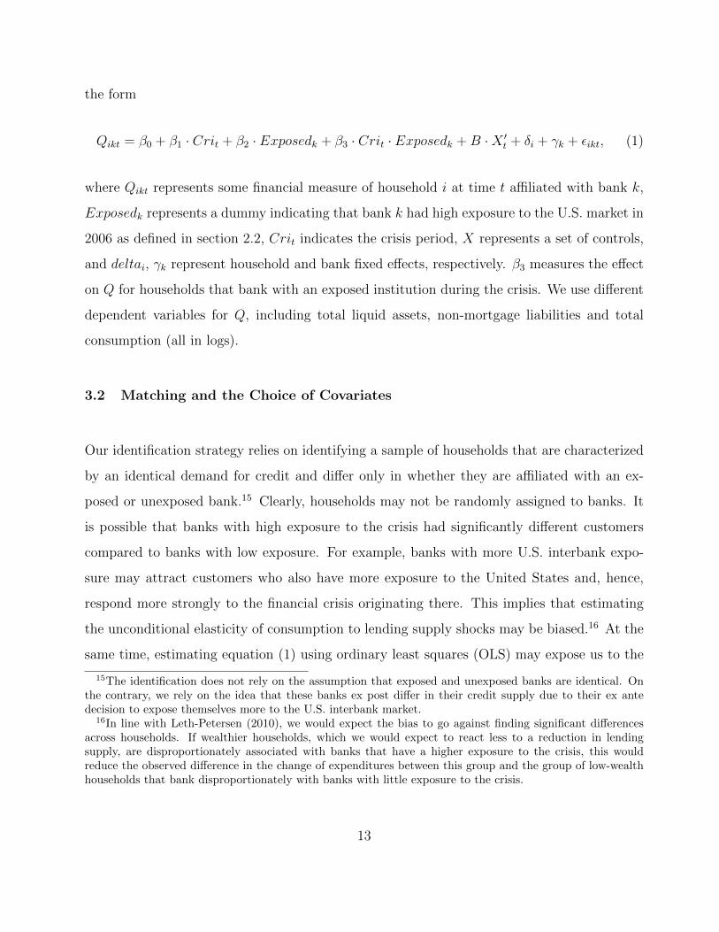
Qikt = β0 + β1 · Crit + β2 · Exposedk + β3 · Crit · Exposedk +B ·X ′t + δi + γk + εikt, (1)
where Qikt represents some financial measure of household i at time t affiliated with bank k,
Exposedk represents a dummy indicating that bank k had high exposure to the U.S. market in
2006 as defined in section 2.2, Crit indicates the crisis period, X represents a set of controls,
and deltai, γk represent household and bank fixed effects, respectively. β3 measures the effect
on Q for households that bank with an exposed institution during the crisis. We use different
dependent variables for Q, including total liquid assets, non-mortgage liabilities and total
consumption (all in logs).
3.2 Matching and the Choice of Covariates
Our identification strategy relies on identifying a sample of households that are characterized
by an identical demand for credit and differ only in whether they are affiliated with an ex-
posed or unexposed bank.15 Clearly, households may not be randomly assigned to banks. It
is possible that banks with high exposure to the crisis had significantly different customers
compared to banks with low exposure. For example, banks with more U.S. interbank expo-
sure may attract customers who also have more exposure to the United States and, hence,
respond more strongly to the financial crisis originating there. This implies that estimating
the unconditional elasticity of consumption to lending supply shocks may be biased.16 At the
same time, estimating equation (1) using ordinary least squares (OLS) may expose us to the
15The identification does not rely on the assumption that exposed and unexposed banks are identical. Onthe contrary, we rely on the idea that these banks ex post differ in their credit supply due to their ex antedecision to expose themselves more to the U.S. interbank market.
16In line with Leth-Petersen (2010), we would expect the bias to go against finding significant differencesacross households. If wealthier households, which we would expect to react less to a reduction in lendingsupply, are disproportionately associated with banks that have a higher exposure to the crisis, this wouldreduce the observed difference in the change of expenditures between this group and the group of low-wealthhouseholds that bank disproportionately with banks with little exposure to the crisis.
13
sensitivity of OLS to differences in the covariate distribution between households affiliated
with high-exposure banks and households affiliated with low-exposure banks.
Instead, we use propensity score matching to obtain estimates of β3. A matching estimator
balances the covariates between the households affiliated with low-exposure banks with those
households affiliated with high-exposure banks without imposing functional form assumptions.
Consider
E[(Q1i,Cri −Q1
i,P re)− (Q0i,Cri −Q0
i,P re)|Exposed = 1, Xi,P re] =
E[(Q1i,Cri −Q1
i,P re)|Exposed = 1, Xi,P re]− E[(Q0i,Cri −Q0
i,P re)|Exposed = 1, Xi,P re], (2)
where E[·] is the expectation operator and (Q1i,Cri − Q1
i,P re) is the change in expenditure
(or consumer credit, liquid assets, etc.) of exposed household i between the pre-crisis and
crisis periods. Equation (2) measures the difference in consumption expenditures between
exposed and unexposed households during the crisis period relative to the non-crisis period.
This corresponds to β3 in equation (1) and is known as the “average treatment effect on the
treated” (ATT).
There is no sample counterpart for the second term on the right-hand side of equation
(2). It is a counterfactual; i.e., the change in consumption expenditure of households affiliated
with an exposed bank had they been affiliated with an unexposed bank. We can, however,
still recover the causal effect β3 if the assignment of a household to a bank is random condi-
tioning on Xi,P re. We follow the matching procedure suggested by Abadie and Imbens (2006)
to estimate the counterfactual. For each household in the exposed group, we obtain the clos-
est four matches from the unexposed group,17 calculate the average level of the log of the
measure of interest (liquid assets, non-mortgage liabilities, consumption), and compare it to
17According to Imbens and Wooldridge (2009), “little is known about the optimal number of matches,or about data-dependent ways of choosing it.” Nevertheless, using more than one match for each treatedobservation seems to improve the Abadie and Imbens (2006) procedure. We choose four matches, given oursample size and the number of households in our control sample.
14

the respective measure by the exposed household. Matching is done with replacement so that
the same unexposed household can be matched with different exposed households. Reusing
observations minimizes the risk that the unexposed households do not look like their exposed
matches, but potentially at the expense of a loss of precision.
Choosing covariates is crucial, but unfortunately there is no formal approach for doing so.
The goal is to compare consumption patterns of households that have identical characteris-
tics that may be related to consumption and borrowing, and that differ only in their choice
of a banking institution (i.e., an exposed vs. an unexposed bank). Therefore, we use stan-
dard household characteristics such as age, family size and marital status, but also financial
characteristics such as home ownership or income.
4 Results
4.1 Propensity Score Estimation and Match Quality Assessment
We estimate a probit model and obtain the probability of banking with an exposed financial
institution (i.e., the propensity score) as a function of home equity, home value, gross income,
age of the head of household, marital status, unemployment status, house size, labor supply,
self-employment, level of education, number of children, a dummy equal to one if the household
lives in a major metropolitan area, a dummy variable indicating whether the household rents, a
dummy variable indicating whether the household’s main language is French, and an indicator
variable controlling for the household’s level of risk aversion.18 In addition, the model includes
18The risk aversion variable is calculated using another new segment added to the CFM in 2007. In this“attitudinal section,” respondents are asked about their agreement/disagreement on a variety of statementsregarding risk tolerance. We place equal weight on two such questions (“I don’t like to invest in the stockmarket because it is too risky” and “I am willing to take substantial risks to earn substantial returns”) tocalculate a risk aversion index. Since the attitudinal questions are available only from 2007 onwards, we usethe 2007 values for our panel households that have also completed the 2007 survey (approximately 65%). Forthe rest of the households, we use the 2008 risk aversion data and implicitly assume that the onset of the crisisdid not drastically change attitudes toward risk.
15

squared continuous variables to allow for a non-linear relation with the dependent variable.
All variables are measured at the pre-crisis period, except risk aversion. As discussed above,
the sample includes 3,804 panel observations where each household is present at least once in
both the pre-crisis (2005-2006) and crisis (2008-2009) periods, and we are able to identify the
household’s main bank and its exposure (along with having data on all of the probit variables
for the pre-crisis period). About 32% of the households are classified as exposed.
The estimation results are reported in Table 3 and suggest that households with an exposed
bank are quite similar to households with an unexposed bank even in the raw data. Only a few
of the determinants are significant. For instance, the probability of banking with an exposed
institution is positively correlated with the share of home equity. However, households that
report higher gross income are less likely to be associated with an exposed bank. The chance
of having an exposed bank is lower for households whose female head participates in the labor
force. Residents of big cities are less likely, and households whose main language is French
are more likely, to bank with an exposed institution. Finally, households that report higher
levels of risk aversion are more likely to bank with an exposed institution.
Since the purpose of the matching procedure is to balance the covariates across the two
groups, we report two-sample t-statistics for all explanatory variables in Table 4. A failure
to reject the test indicates that, on average, there is no difference between households that
bank with an exposed vs. an unexposed financial institution. The reported t-tests show no
evidence of differences in the characteristics of the two groups. Finally, the validity of the
matching estimator depends on the presence of common support for the propensity scores of
exposed vs. unexposed households. As shown in Figure 4, there is ample common support
between exposed and unexposed households, alleviating these concerns.19
19In section 5.1 we perform further analysis that measures the sensitivity of our method to hidden bias(“Rosenbaum bounds”).
16

4.2 Main Results
This section reports our main results of estimating the average effect on the variables of
interest (consumption expenditure, non-mortgage liabilities and liquid assets) of banking with
an exposed institution. We start with effects in the overall sample and subsequently move to
some subsamples of households that may suffer more from a reduction in credit supply. Ideally,
we would compare consumption patterns between the two groups in the pre-crisis and crisis
periods, but since the survey starts covering consumption in 2008, we observe this variable only
in the crisis period. Hence we initially focus on the changes in liquid assets and non-mortgage
liabilities, which are reported throughout the analysis period, and differences in the level of
consumption expenditures during the crisis between exposed and unexposed households.20
As long as our matching procedure is successful, differences in crisis consumption should be
informative about the effect of being with an exposed bank. We report the results for imputed
consumption using a DID framework in the robustness section.
The results in Table 5 indicate that, overall, there was a significantly negative effect on the
level of liquid assets and non-mortgage liabilities for the exposed households (i.e., negative
and significant ATTs), along with an insignificant effect on consumption during the crisis.
First, we note that exposed households are indistinguishable from unexposed households in
the 2005-2006 period (i.e., pre-crisis). The differences between the groups with respect to
liquid assets and non-mortgage liabilities are statistically insignificant. However, during the
2008-2009 period (i.e., the crisis), exposed households report relatively lower log levels of non-
mortgage liabilities (the ATT is -0.462, which translates to a 37% difference) and liquid assets
(an ATT of -0.428, or a 34% difference). The DID is statistically significant at the 5% and 1%
levels, respectively. Households banking with exposed institutions report significantly lower
non-mortgage liabilities compared to households with unexposed institutions that otherwise
20The difference in the level of consumption between exposed and unexposed households can be representedas (Q1
i,Cri −Q0i,Cri), which is easily obtained by rearranging the terms in equation (2).
17

exhibit identical observables. Second, there is no evidence that consumption patterns between
the two groups are different in the crisis period. This is the central finding of our study:
faced with banks’ inability to lend, customers of affected institutions, rather than reduce
consumption, draw down their liquid assets. This is consistent with consumption smoothing
in the face of temporary shocks, as predicted by the literature (e.g., Jappelli and Pistaferri
(2010)). It also suggests that Canadian households perceive their inability to obtain credit as
temporary, rather than permanent. We explore some of the macroeconomic consequences of
this finding below.21
Our next step addresses two important concerns that arise out of the link between expo-
sure to the crisis and the level of non-mortgage liabilities. First, we would like to provide
additional evidence that what we are observing is a supply shock and not a demand-driven
decrease in borrowing by exposed households. Although the nature of our matching procedure
makes such a demand shock unlikely, it is important to ascertain a reduction in bank lending.
Second, in light of the extensive literature on credit constraints and consumption patterns,
we further investigate whether the lower levels of borrowing are more pronounced among ex-
posed households that were more likely to become credit constrained during the crisis. If the
likelihood of becoming credit constrained during the crisis plays a role in the borrowing pat-
terns, then accounting for this variable can improve our matching procedure and allow us to
uncover any consumption effects that might exist among financially constrained and exposed
households.
We address these concerns by looking for systematic differences across the two groups of
households while controlling for their likelihood of becoming credit constrained. In order to
identify households that are more likely to be financially constrained, we consider all house-
holds who are homeowners and have at least a 20 per cent equity stake in their house during
21As a robustness check, we also estimate equation (1) by OLS using the same covariates as in the probitanalysis (Table 3) with clustered standard errors at the bank level. We obtain results that are statisticallyand economically consistent with the ATTs reported in Table 5.
18

the pre-crisis period. Within this subsample, we define financially constrained households as
those without a home equity line of credit (HELOC). These are households that have equity
in their homes, but they do not have the means to extract it.22 This makes such households
more constrained compared to households with both the equity and the means to extract
it. During times of financial stress, banks might be reluctant to grant new HELOCs even to
households with sufficient equity, but they will be much less likely to prevent customers from
drawing down existing HELOCs.
We use a HELOC-based definition of financial constraint, since HELOCs have higher credit
limits, more-flexible payment terms and lower borrowing rates than other kinds of revolving
consumer credits (DBRS, 2012). Moreover, Hurst and Stafford (2004) argue that households
use their housing equity as a “financial buffer,” which is accessed via HELOCs or refinancing
when needed. In our context, it is likely that at least some Canadian households attempted to
extract home equity during the crisis period. Therefore, any differences in the ATTs for non-
mortgage liabilities between constrained and unconstrained households will be additional proof
of a supply effect. If the link between exposure and non-mortgage liabilities discussed above
is driven by demand, then we should expect to see negative ATTs on non-mortgage liabilities
for both constrained and unconstrained households. However, if a negative treatment effect is
observed for the constrained households only, then we can argue that all exposed households
attempted to extract home equity during the crisis period, but only those with an existing
HELOC were able to do so.23 The implication is that exposed households without HELOCs
were unable to obtain a HELOC, making a credit supply shock the likely explanation.
Once the households are classified, we follow the same procedure and match on propen-
22Given that our constraint definition is based on having, and potentially extracting, home equity, weeliminate renters, households with less than 20% equity (the minimum required by regulators to qualify for aHELOC) and households that switch home ownership status between the pre-crisis and crisis periods.
23We do not have a stance on whether households attempted to access home equity in order to smooth incomeshocks or to take advantage of stimulus programs such as “home renovation tax credit,” low interest rates onnew automobiles or other programs that were available in Canada during the crisis. In other words, we donot attempt to distinguish between the “financial motivation” and the “consumption-smoothing motivation”discussed in Hurst and Stafford (2004).
19

sity score and credit constraint. Estimates of the ATTs for constrained vs. unconstrained
households are reported in Table 6. Considering financially constrained households first, as
before, the two groups (exposed vs. unexposed) are indistinguishable in the pre-crisis period,
since there are no significant differences in the levels of liquid assets and non-mortgage liabil-
ities. However, during the crisis, the differences between the two groups become significant
as constrained exposed households report lower log levels of liquid assets (the ATT implies
a 26% difference) and non-mortgage liabilities (52%), with similar statistical significance for
the DID estimators. As for consumption, we find no evidence of differences between the two
groups during the crisis period. The results suggest that while constrained households are
more affected by the treatment (being with an exposed bank) in terms of their non-mortgage
liabilities, they are able to compensate for the inability to borrow by drawing down liquid
assets. Consumption is unaffected even for these households.
Our findings regarding non-mortgage liabilities and liquid assets strongly point to the
presence of a supply shock that affected financially constrained households. While exposed but
unconstrained households were able to draw down their HELOCs, exposed and constrained
households were unable to obtain the means to extract their home equity. Subsequently,
constrained and exposed households used liquid assets to smooth their consumption, while
unconstrained households’ liquid assets remained relatively unchanged between the pre-crisis
and crisis periods. We conjecture that the ability of constrained and exposed households to
draw down their liquid assets also explains the absence of a consumption effect in the face of
a negative credit supply shock.
Despite the absence of a consumption effect in our analysis so far, it is still possible that
banking with an exposed financial institution can lead to lower consumption expenditures for
households that are both illiquid and exposed. Given that exposure is associated with lower
levels of non-mortgage liabilities, households that have little or no liquid assets to compensate
may end up lowering consumption. We investigate this possibility by concentrating on the
20
distribution of the ATT on total consumption for our baseline analysis (which does not account
for the financial constraint variable). Although this treatment effect is small and negative, its
distribution (plotted in Figure 5) shows a left tail with large negative values. It is possible that
the matches with such negative treatment effects on consumption spending involve households
with low liquid asset holdings.
Our specific approach involves a comparison between the matches that are in the bottom
quartile of the treatment effect on total consumption expenditure and the rest of the sample.
Splitting the matches into these two groups enables us to calculate average treatment effects
within each sample, and allows us to determine whether ATTs of other variables are also
different for the matches with large and negative treatment effects on total consumption
spending. In addition, we can also determine whether the pre-crisis liquid asset holdings of
the exposed households involved in such matches are significantly lower than the rest of the
exposed households.
The results of this analysis are reported in Table 7 and they broadly confirm that low levels
of liquid asset holdings are associated with a negative treatment effect on consumption expen-
diture. The ATTs on total consumption (by design), durables and luxuries are significantly
more negative for the bottom quartile of the total consumption treatment effect distribution,
and the differences in the ATTs between the two groups are statistically significant. The ATTs
on the change in non-mortgage liabilities and liquid assets, on the other hand, are the same
across the two groups, suggesting that the exposed households in both groups experienced a
similar (negative) credit supply shock. The difference in their consumption spending can be
explained by the lower pre-crisis liquid asset holdings of the exposed households in the bottom
quartile. This difference in liquid asset holdings (which is statistically significant) explains
why the exposed households in the bottom quartile were unable to compensate for the credit
supply shock by using their liquid assets.
21

4.3 Economic Magnitudes
In this section, we report the micro- and macroeconomic effects of our findings. The ATT
in non-mortgage liabilities between exposed and matched households of -0.462 from Table 5
translates into a 37% difference between the levels of exposed and matched households’ non-
mortgage liabilities during the crisis. Since the average level of non-mortgage liabilities held
by matched households during the crisis is 16,451 Canadian dollars (CAD), this implies an
average difference of 6,086 CAD in non-mortgage liabilities between an exposed household
and a matched household. Correspondingly, the ATT of -0.428 for liquid assets in Table 5
translates into a 34% difference in the levels of liquid assets between exposed and matched
households. The average level of liquid assets held by matched households during the crisis is
17,503 CAD, implying an average difference of 5,951 CAD between an exposed household and
a matched household. Hence, the CAD reduction in borrowing is almost completely offset by
a corresponding drawdown of liquid assets, resulting in a zero consumption effect. This figure
is also in line with the lack of an overall consumption effect, given that the average liquid
asset holdings of exposed households before the crisis are 11,956 CAD.24
Next, in order to obtain some sense of the macroeconomic magnitudes, we use the survey
weights of exposed households to create the population of affected households during the
crisis period (i.e., 2008-2009). This is done quarterly, based on when the exposed household
completed the survey. We sum the weights for each quarter and multiply this sum with the
average difference in non-mortgage liabilities (6,086 CAD) to create the level of quarterly lost
lending. Finally, we add this forgone lending to the actual outstanding level of credit in each
quarter during the crisis and come up with a counterfactual (i.e., the level of actual plus
cumulatively-forgone credit), and plot the result in Figure 6. By construction, early in 2008
24We observe similar patterns if we use matched households’ median holdings of non-mortgage debt andliquid assets during the crisis. The implied difference is 1,739 CAD for non-mortgage liabilities (37% of 4,700CAD) and 2,380 CAD for liquid assets (34% of 7,000 CAD). Again, the implied differences in non-mortgageliabilities and liquid assets are quite comparable and, since the median liquid asset holdings among exposedhouseholds in the pre-crisis period are 4,300 CAD, a zero consumption effect is not very surprising.
22

the forgone credit tends to be small, but it grows as we approach the latter stages of 2009.
Throughout the two-year period, the cumulative loss in lending adds up to about 8.1 billion
CAD, or about 2.2% of total outstanding non-mortgage credit at the end of 2009.
A different approach to assess the macroeconomic impact of our results is to compare
the ability of a median Canadian household to withstand a credit supply shock with that
of a median U.S. household. In the above analysis, we show that in the pre-crisis period,
the median exposed Canadian household reports 4,300 CAD of liquid assets. Using a similar
approach and utilizing the 2007 Survey of Consumer Finances, we calculate the liquid asset
holdings of a median U.S. household at 3,415 US dollars (USD). This suggests that when faced
with a similar transitory shock (i.e., if the median credit supply drops by 1,739 USD), U.S.
households will exhaust their liquid asset 20% sooner.
5 Robustness
5.1 Rosenbaum Bounds
Propensity score matching estimators may not be consistent if the assignment to treatment
is endogenous (Rosenbaum (2002)). Unobserved variables that affect the assignment to ex-
posed versus unexposed banks may also be related to the outcome variables; i.e., consumption,
liabilities or liquid assets. Further, the matching is based on the conditional independence as-
sumption, which states that all variables should be simultaneously observed both influencing
the participation decision (propensity to be with an exposed bank, the treatment) and out-
come variables (non-mortgage liabilities, consumption, liquid assets). In order to estimate the
extent to which such “selection on unobservables” may bias our qualitative and quantitative
inferences about the effects, we conducted the sensitivity analysis as outlined in Rosenbaum
(2002). Rosenbaum bounds assess how strongly an unmeasured variable would have to impact
23
on the selection process to invalidate the matching analysis. This does not test the uncon-
foundedness assumption directly, but rather provides evidence on the degree to which the
results hinge on this untestable assumption.
The Rosenbaum bound can be calculated using the probability for a household to bank
with an exposed bank (i.e., receive the “treatment”):
Pi = P (Exposed = 1|Xi,P re, ui) = F (β ·Xi,P re + γ · ui),
where Xi,P re are observed characteristics, ui is the unobserved variable and F is a cumulative
density function. γ measures the impact of the unobserved variable ui on the decision to
bank with an exposed bank. Next, consider a matched pair of households that have the exact
same characteristics (Xi,P re = Xj,Pre). If there is no hidden bias through ui, then γ = 0
and the log-odds ratio Pi/Pj = 1. However, if there is hidden bias, then Pi/Pj 6= 1, and
the Rosenbaum bounds calculate the upper bound of the bias that can be tolerated without
changing the statistical significance of the treatment effect.25
Our estimates of Rosenbaum bounds are around 1.15 for all of our outcome variables. This
implies that any hidden bias that exists must cause the log-odds ratio of being assigned to an
exposed bank to differ between exposed and unexposed households by a factor of about 1.15.
The magnitude of hidden bias that might call our findings into question can be illustrated
using the methodology outlined in Barath et al. (2011). If a logistic regression is utilized,
then the ratio of propensities will change by a factor of 1.15 = exp(βk · sk · n), where βk
is the logit coefficient for covariate k, sk is covariate k’s standard deviation and n is the
number of standard deviations that covariate k has to change by in order for the ratio of
propensities to increase to 1.15. Therefore, we can solve for n for each of the continuous
covariates in our model and determine how large an average change in these covariates is
25For a more detailed technical discussion of Rosenbaum bounds, please see Barath et al. (2011) and Fung,Huynh and Sabetti (2012), who also provide applications of Rosenbaum bounds in a context similar to ours.
24

required in order to mimic the effect of a hidden bias. For most of our covariates, we observe
that a large change would be required (a +88% change in House Value and a +32.5% change
in Home Equity/House Value). The changes required for Gross Income and Age are smaller
at -7.8% and -8.4%, respectively. Nevertheless, these required changes are also non-trivial
and are unlikely to be plausible. Therefore, we conclude that it is unlikely that such powerful
unobserved covariates exist as to render our estimates invalid.
5.2 Imputing Consumption Data
In our main empirical analysis, we are unable to calculate a true difference-in-differences term
for spending (total, durables or luxury), due to the lack of consumption data in the CFM for
the pre-crisis period. It is, however, possible to impute consumption using income and wealth
data in a manner similar to Browning and Leth-Petersen (2003). Specifically, we use their
“accounting imputation” method, which specifies consumption as
ct = yt −∆Wt +∑k
(pkt − pkt−1)Akt−1, (3)
where ct is consumption, yt is disposable income and ∆Wt is the change in wealth between
t−1 and t. Akt−1 is the amount of asset k held by the household at time t−1 and the term in
parentheses is the change in the price of asset k between t− 1 and t (capturing capital gains).
Imputing consumption using equation (3) requires the addition of another time period to
our CFM panel sample. Accordingly, we further limit our sample to households that complete
the CFM survey in 2003 or 2004, 2005 or 2006, and 2008 or 2009. This reduces our sample to
1,660 households (of which 532 are exposed).
We then make some adjustments to equation (3) in order to make the imputation feasible.
25
Unlike the data used by Browning and Leth-Petersen (2003), the CFM reports gross income.
We use federal and provincial income tax rates to approximate disposable income for each
household. However, since we are unable to account for tax credits and capital gains taxes,
this is likely to yield a noisy disposable income variable. Furthermore, given the unavailability
of price data for the financial assets held by the CFM respondents (and similar to Browning
and Leth-Petersen (2003)), we ignore the “capital gains” component of equation (3).
Regarding household wealth (Wt), we consider two approaches:
Basic Wealth = Checking Account Balances + Savings Account Balances + GIC Balances ,
Complete Wealth = Checking Account Balances + Savings Account Balances + GIC Balances
+ House Value + Auto Value + Bond Holdings + Stock Holdings
+ Mutual Fund Holdings .
Basic Wealth is included in our analysis given our concerns related to the fluctuations
in the prices of stocks and bonds during our sample period (especially the crisis period).
Using the two imputed consumption measures implied by these wealth measures (“basic”
vs. “complete”), we estimate treatment effects on imputed consumption during the crisis,
the pre-crisis period and the change in imputed consumption. Since imputed consumption
exists for only a part of our sample, we perform a new matching procedure to ensure that all
of the unexposed households that get matched to an exposed household have valid imputed
consumption observations.26
The results of our baseline matching and our analysis using financially constrained house-
holds are reported in Tables 8 and 9. The lack of any significant treatment effects for pre-crisis
26Another approach would be to keep our original matches (based on our full sample) and calculate atreatment effect using only the matches for which imputed consumption data exist for the exposed householdand at least one of the matched households. Following this approach does not change our findings.
26

or crisis consumption levels broadly confirms our conclusions of consumption smoothing by
exposed households, despite lower credit supply during the crisis period.
5.3 Alternative Exposure Measure
Although our main empirical analysis used interbank deposits from the United States as a
measure of exposure to the crisis, it is possible to construct another exposure measure based
on the existing literature. As discussed by Ivashina and Scharfstein (2010), banks that were
more dependent on wholesale funding prior to the crisis reduced their lending more during
the crisis than did banks relying on retail deposits. Therefore, categorizing Canadian banks
according to their wholesale funding can give us an alternative measure for Exposure. For this
categorization, we define wholesale funding as follows:
WSF =Interbank Deposits + Acceptances + Repurchase Arrangements
Total Assets.
The banks (and credit unions) in our sample are then divided into “exposed” vs. “unex-
posed” categories in a manner similar to our main analysis above. We look for a “natural
break” in WSF, which occurs in two places. The first break occurs around 1%, since some
of the smaller banks and credit unions use little or no wholesale funding. However, given the
distribution of the CFM respondents’ main banks, categorizing all banks with WSF ≥ 1%
as “exposed” would result in almost all households in our sample being categorized as such.
The second natural break occurs around 15%, with WSF ranging from 0% to approximately
13.5% for one group of banks and 17.5% to approximately 35% for another group of banks.
We use this second natural break and categorize all banks with WSF ≥ 15% as “exposed.”27
27For data confidentiality reasons, we are unable to discuss the similarities and differences in the exposurecategorization of the banks in our sample under our two different measures. This is due to the fact that,although most of the data used to calculate WSF are publicly available, the interbank deposits from the U.S.data used in our main empirical analysis are confidential. We can, however, report that the two categorizationsare not identical, but there is considerable overlap between the two.
27

This categorization results in 1,658 exposed and 2,119 unexposed households.28
The balance of covariates between the exposed and matched sample (Table 10) indicates
that there are no statistically significant differences between the exposed and matched house-
holds. Table 11 shows the results of our baseline analysis. The findings are quite similar to
our main empirical analysis above, with one exception, namely that the average treatment
effect for the change in non-mortgage liabilities is negative but insignificant. Finally, Table 12
displays the results of our analysis based on the distribution of the treatment effect on total
consumption. The findings confirm our earlier conclusions, given that the exposed households
with the most negative treatment effects on consumption also had lower levels of liquid assets
prior to the crisis. Therefore, when faced with a credit shock (which again appears to be the
same across all exposed households), these households were unable to maintain consumption.
5.4 Further Robustness Issues
In this section, we address two concerns regarding our identification. First, we explore the
potential effect of households switching between exposed and unexposed banks, and second,
we address concerns that our results may be driven by regional differences in macroeconomic
performance in Canada. We measure the household’s bank before the crisis and implicitly
assume that the household stays with this bank throughout the sample period. However,
households can switch banks and, if credit is unavailable at the incumbent bank, obtain the
desired levels of credit from a competitor that may be unexposed. If households switched banks
during the crisis, this could result in a downward bias in the ATTs. We assess the magnitude
of this problem using two approaches: one that is based on actual switching behavior (i.e., ex
post) and another that is based on a tendency to switch (i.e., ex ante).
28The total number of households is lower for this specification, since we are unable to calculate WSF forsome credit unions (unlike information on their interbank deposits from the United States, which was providedto us by their regulators).
28
In the first approach, we calculate the probability of households classified as exposed in
the pre-crisis period switching to an unexposed institution in the crisis period. We find that
only 4% did so. This low number is consistent with the previous evidence in Allen et al.
(2008). Our results are unaffected when we drop the switching households from our sample.
Our second approach utilizes a set of specific survey questions that qualitatively measure
households’ propensity to switch institutions. We construct an ‘intention to switch’ index
(ranging from 0 to 1) using six attitudinal questions.29 We find very little cross-sectional
variation in this index, since most respondents are at the mean of 0.48, which indicates that
they are neither very likely nor very unlikely to switch banks.
A further concern is that our matching procedure could produce matches of households
in different parts of Canada. This could create a bias in the treatment effects. For example,
Alberta had robust growth prior to the financial crisis due to high natural resource prices.
However, it was hit hard when natural resource prices dropped during the crisis. If this
exogenous variation is correlated with a higher exposure of banks in this region to the United
States, this could result in the confounding of the supply effect we attempt to estimate with
demand factors.30 We perform a number of calculations to address this concern. First, we
estimate ATT effects on the unemployment of households. If matched households lived in
regions that had better economic performance, we should be able to detect differences in
unemployment rates among exposed and unexposed households during the crisis. We do not
find such an effect. Second, we check for the proportion of exposed households that were
matched to at least one household in the same region.31 This proportion is 66%, suggesting
that, in general, we do a decent job of matching households within regions. Finally, suppose
29The questions include “there are big differences between financial institutions,” “I prefer to deal withpeople when I bank, rather than using an automated machine or the Internet,” “I always actively look fornew offers and check that I am getting the best deal from my financial institution.” Each question was to beanswered on a score from 1 to 10 by the respondent.
30Similarly, it is possible that exposed households are more likely to work for U.S. firms or in parts of Canadathat are otherwise more integrated with the United States.
31These regions are Atlantic Canada (consisting of four provinces), Quebec, Ontario, the Prairie provinces(consisting of two provinces), Alberta and British Columbia.
29

we were unable to pick up all heterogeneity in this regard. This would lead us to overstate
differences in non-mortgage liabilities and consumption. However, we do not find a difference
in consumption between exposed and matched households. Instead, we find significant effects
on liquid assets. If an important part of our results were driven by a demand effect, we should
find significant differences in consumption expenditure and insignificant differences in crisis
levels of liquid assets. This, however, is not what we find.
6 Conclusion
In this paper we seek to empirically establish a link between bank financial distress, credit
supply to households and household consumption expenditures. If financial distress in bank-
ing adversely affects household consumption due to, for instance, exacerbating household
credit constraints, this may have first-order macroeconomic consequences. We find evidence
in favour of a lending supply effect: distressed banks reduce lending, especially to financially
weaker households. There is no corresponding effect, however, on consumption expenditure.
Households smooth their consumption by drawing down their liquid assets. Our results are
consistent with the interpretation that households perceive an adverse lending supply shock
as temporary.
The results have important policy implications. For example, they suggest that households
will not reduce their consumption based on temporary shocks, as long as they can draw on
liquid assets. This stands in stark contrast to recent results for firms (Campello, Graham
and Harvey (2010); Puri, Rocholl and Steffen (2011)), where the same shock affected firm
investment and employment decisions. At the same time, households, by drawing down liquid
assets, may have exacerbated the funding problems of banks. Further, the significant decline in
aggregate consumption expenditures in Canada during the financial crisis was largely unrelated
to credit supply, but rather consumption demand. This is striking, given that the Canadian
economy did not experience the bursting of a housing bubble and was, by most accounts,
30
not strongly affected in terms of fundamentals. The results reported in this paper suggest
that there was a “pure” contagion effect at work: Canadian households reduced consumption
expenditure because they were unsure about how the crisis in the United States and elsewhere
would affect their future economic well-being (the “CNN effect”).
References
Abadie, A., and G. W. Imbens. 2006. “Large Sample Properties and Matching for Average
Treatment Effects.” Econometrica, 74: 235–267.
Abdallah, C., and W. Lastrapes. 2012. “Home Equity Lending and Retail Spending: Evi-
dence from a Natural Experiment in Texas.” American Economic Journal: Macroeconomics,
4(4): 94–125.
Agarwal, S., C. Liu, and N. Souleles. 2007. “The Reaction of Consumer Spending and
Debt to Tax Rebates – Evidence from Consumer Credit Data.” Journal of Political Econ-
omy, 115(6): 986–1019.
Alessie, R., S. Hochguertel, and G. Weber. 2005. “Consumer credit: Evidence from
Italian micro data.” Journal of the European Economic Association, 3(1): 144–178.
Allen, J., R. Clark, and J. Houde. 2008. “Market Structure and the Diffusion of E-
Commerce: Evidence from the Retail Banking Industry.” Bank of Canada Working Paper
No. 2008-32.
Barath, S., S. Dahiya, A. Saunders, and A. Srinivasan. 2011. “Lending Relationships
and Loan Contract Terms.” Review of Financial Studies, 24: 1141–1203.
Browning, M., and S. Leth-Petersen. 2003. “Imputing Consumption from Income and
Wealth Information.” Economic Journal, 113: F282–F301.
31
Campello, M., J. Graham, and C. Harvey. 2010. “The Real Effects of Financial Con-
straints: Evidence from a Financial Crisis.” Journal of Financial Economics, 97: 470–487.
Cohen-Cole, E., B. Duygan-Bump, J. Fillat, and J. Montoriol-Garriga. 2008. “Look-
ing Behind the Aggregates: A Reply to ‘Facts and Myths About the Financial Crisis of
2008’.” Federal Reserve Bank of Boston Quantitative Analysis Unit Working Paper No.
08-5.
Dell’Ariccia, G., E. Detragiache, and R. Rajan. 2008. “The Real Effect of Banking
Crises.” Journal of Financial Intermediation, 17: 89–112.
Dominion Bond Rating Service (DBRS). 2012. “Rating Canadian Home Equity Lines
of Credit (HELOCs).”
Fung, B. S. C., K. Huynh, and L. Sabetti. 2012. “The Impact of Retail Payment
Innovations on Cash Usage.” Bank of Canada Working Paper No. 2012-14.
Gozzi, J., and M. Goetz. 2010. “Liquidity Shocks, Local Banks, and Economic Activity:
Evidence from the 2007-2009 Crisis.” Working paper, SSRN 1709677.
Gross, D. B., and N. S. Souleles. 2002. “Do Liquidity Constraints and Interest Rates
Matter for Consumer Behavior? Evidence from Credit Card Data.” Quarterly Journal of
Economics, 117(1): 149–185.
Hurst, E., and F. Stafford. 2004. “Home Is Where the Equity Is: Mortgage Refinancing
and Household Consumption.” Journal of Money, Credit and Banking, 36(6): 985–1014.
Imbens, G. W., and J. M. Wooldridge. 2009. “Recent Developments in the Econometrics
of Program Evaluation.” Journal of Economic Literature, 47(1): 5–86.
Ivashina, V., and D. Scharfstein. 2010. “Bank Lending During the Financial Crisis of
2008.” Journal of Financial Economics, 97(3): 319–338.
32

Jappelli, T., and L. Pistaferri. 2010. “The Consumption Response to Income Changes.”
Annual Review of Economics, 2: 479–506.
Johnson, D. S., J. A. Parker, and N. S. Souleles. 2006. “Household Expenditure and
the Income Tax Rebates of 2001.” American Economic Review, 96(5): 1589–1610.
Kartashova, K., and B. Tomlin. 2013. “House Prices, Consumption and the Role of Non-
Mortgage Debt.” Bank of Canada Working Paper No. 2013-2.
Leth-Petersen, S. 2010. “Intertemporal Consumption and Credit Constraints: Does Total
Expenditure Respond to an Exogenous Shock to Credit?” American Economic Review,
100(3): 1080–1103.
Meghir, C., and L. Pistaferri. 2011. “Earnings, Consumption and Life Cycle Choices.”
Handbook of Labor Economics, 4(Part B): 773–854.
Mian, A., and A. Sufi. 2010. “Household Leverage and the Recession of 2007 to 2009.”
NBER Working Paper No. 15896.
Peek, J., and E. S. Rosengren. 1997. “The International Transmission of Financial Shocks:
The Case of Japan.” American Economic Review, 87(4): 495–505.
Peek, J., and E. S. Rosengren. 2000. “Collateral Damage: Effects of the Japanese Bank
Crisis on Real Activity in the United States.” American Economic Review, 90(1): 30–45.
Peek, J., E. S. Rosengren, and G. M. B. Tootell. 2003. “Identifying the Macroeconomic
Effect of Loan Supply Shocks.” Journal of Money, Credit, and Banking, 35(6): 931–946.
Puri, M., J. Rocholl, and S. Steffen. 2011. “Global Retail Lending in the Aftermath of
the US Financial Crisis: Distinguishing between Supply and Demand Effects.” Journal of
Financial Economics, 100: 556–578.
Rosenbaum, P. R. 2002. Observational Studies. 2nd ed., New York, NY: Springer.
33
Santos, J. 2011. “Bank corporate loan pricing following the subprime crisis.” Review of
Financial Studies, 24(6): 1916–1943.
Stiglitz, J., and A. Weiss. 1981. “Credit rationing in markets with imperfect information.”
American Economic Review, 71(3): 393–410.
Telyukova, I. A., and R. Wright. 2008. “A Model of Money and Credit, with Application
to the Credit Card Debt Puzzle.” Review of Economic Studies, 75(2): 629–647.
34

Figure 1: Total consumption expenditures, durable consumption expenditures and the growthrate of household credit in Canada (2007Q1-2010Q4)
780
800
820
840
860
Tot
al C
onsu
mpt
ion
(bill
ions
CA
D)
2007Q1 2008Q1 2009Q1 2010Q1 2011Q1
(a) Total Consumption Expenditure
0.01
50.
020.
025
0.03
HH
Cre
dit G
row
th R
ate
2007Q1 2008Q1 2009Q1 2010Q1 2011Q1
(b) Growth Rate Household Credit
115
120
125
130
Dur
able
s C
onsu
mpt
ion
(bill
ions
CA
D)
2007Q1 2008Q1 2009Q1 2010Q1 2011Q1
(c) Durable Consumption Expenditure
35
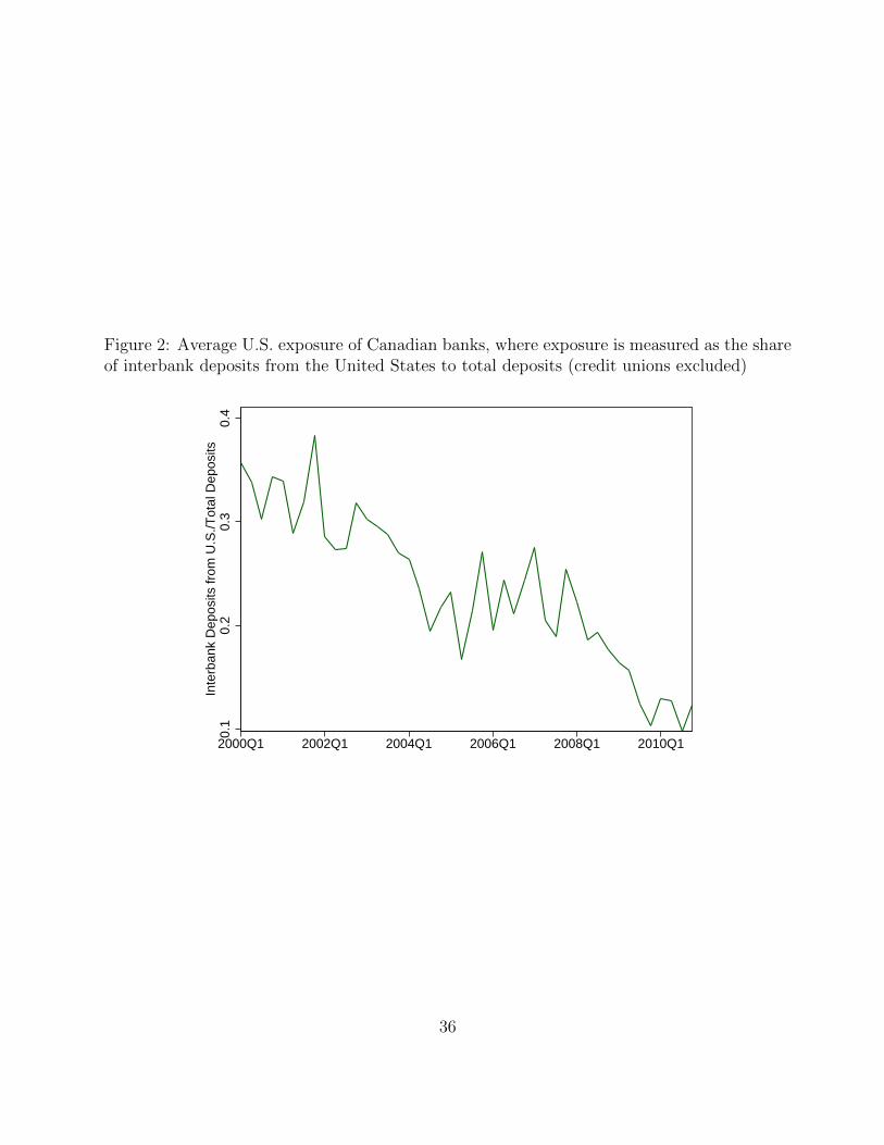
Figure 2: Average U.S. exposure of Canadian banks, where exposure is measured as the shareof interbank deposits from the United States to total deposits (credit unions excluded)
0.1
0.4
0.3
0.2
Inte
rban
k D
epos
its fr
om U
.S./T
otal
Dep
osits
2000Q1 2004Q12002Q1 2006Q1 2008Q1 2010Q1
36
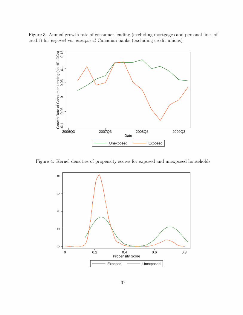
Figure 3: Annual growth rate of consumer lending (excluding mortgages and personal lines ofcredit) for exposed vs. unexposed Canadian banks (excluding credit unions)
0-0
.10.
050.
1-0
.05
0.15
Gro
wth
Rat
e of
Con
sum
er L
endi
ng (
no H
ELO
Cs)
2006Q3 2007Q3 2008Q3 2009Q3Date
Unexposed Exposed
Figure 4: Kernel densities of propensity scores for exposed and unexposed households
02
46
8
0 0.2 0.4 0.6 0.8Propensity Score
Exposed Unexposed
37

Figure 5: Kernel density of the treatment effect on total consumption
00.
20.
40.
6
-3 -2 -1 0 1 2Treatment Effect on Total Consumption
Figure 6: Expected vs. actual CPI adjusted levels (in billions of 2002 Canadian dollars) ofnon-mortgage liabilities
240
260
280
300
320
340
Bill
ions
of 2
002
CA
D
2007Q3 2009Q32009Q12008Q32008Q1
Actual Expected
38
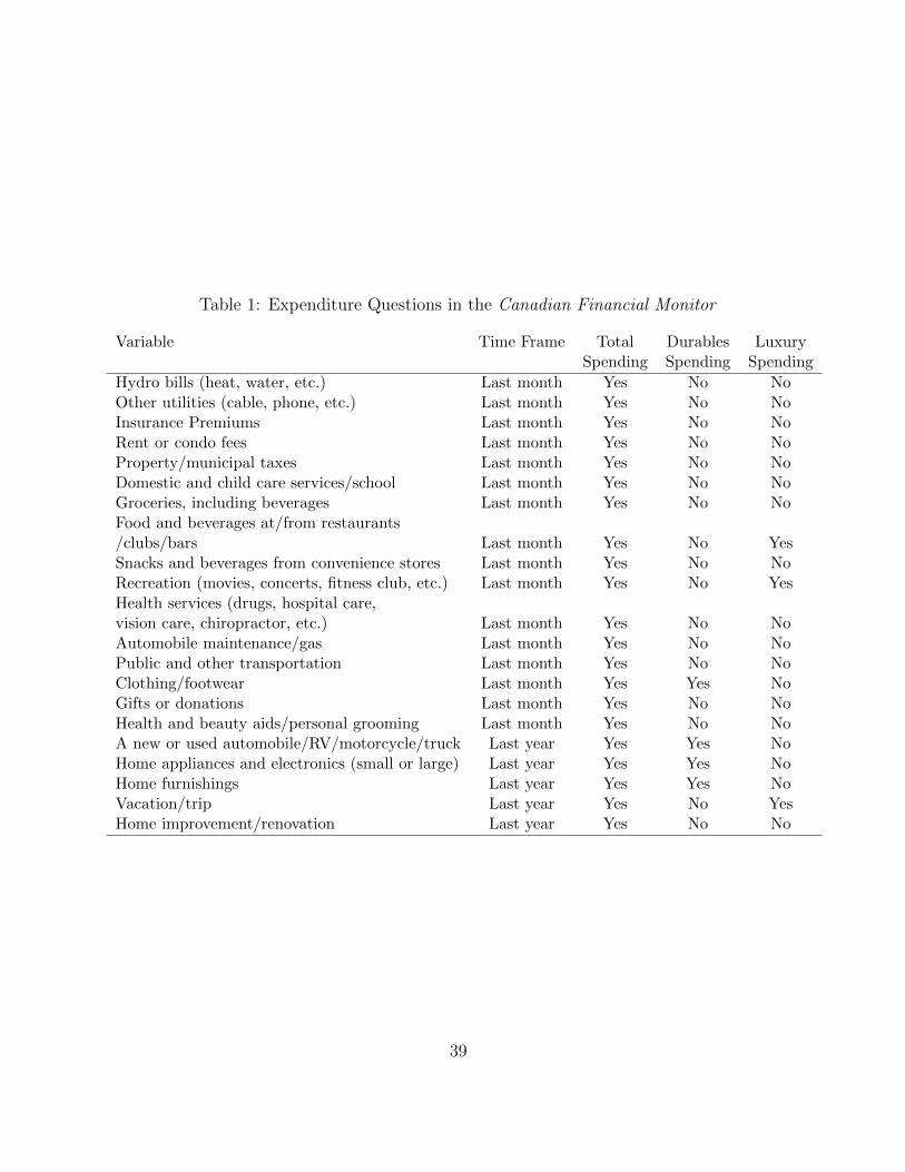
Table 1: Expenditure Questions in the Canadian Financial Monitor
Variable Time Frame Total Durables LuxurySpending Spending Spending
Hydro bills (heat, water, etc.) Last month Yes No NoOther utilities (cable, phone, etc.) Last month Yes No NoInsurance Premiums Last month Yes No NoRent or condo fees Last month Yes No NoProperty/municipal taxes Last month Yes No NoDomestic and child care services/school Last month Yes No NoGroceries, including beverages Last month Yes No NoFood and beverages at/from restaurants/clubs/bars Last month Yes No YesSnacks and beverages from convenience stores Last month Yes No NoRecreation (movies, concerts, fitness club, etc.) Last month Yes No YesHealth services (drugs, hospital care,vision care, chiropractor, etc.) Last month Yes No NoAutomobile maintenance/gas Last month Yes No NoPublic and other transportation Last month Yes No NoClothing/footwear Last month Yes Yes NoGifts or donations Last month Yes No NoHealth and beauty aids/personal grooming Last month Yes No NoA new or used automobile/RV/motorcycle/truck Last year Yes Yes NoHome appliances and electronics (small or large) Last year Yes Yes NoHome furnishings Last year Yes Yes NoVacation/trip Last year Yes No YesHome improvement/renovation Last year Yes No No
39

Table 2: Summary Statistics for Consumption, Credit and Liquid Asset Variables
Exposed Households Unexposed HouseholdsVariable Mean Median Std. Dev. Mean Median Std. Dev.
Crisis Period (2008-2009)
Total Consumption 33746 29472 21358 35010 31973 20285Durables Spending 5313 2248 6995 5062 1971 7034Luxury Spending 3954 2341 4554 4573 2941 4742
Non-Mortgage Liabilities 15380 3250 26244 18153 4500 29765Liquid Asset Holdings 14006 5300 23676 19716 7750 24067
Pre-Crisis Period (2005-2006)
Non-Mortgage Liabilities 15985 4550 27108 18885 6250 31697Liquid Asset Holdings 11958 4300 21307 16442 6250 27803
40
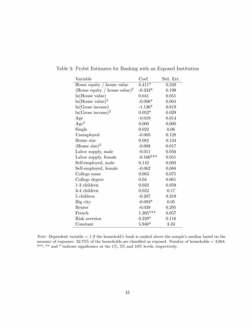
Table 3: Probit Estimates for Banking with an Exposed Institution
Variable Coef. Std. Err.
Home equity / house value 0.411* 0.249(Home equity / house value)2 -0.332* 0.199ln(House value) 0.041 0.051ln(House value)2 -0.006* 0.004ln(Gross income) -1.136* 0.619ln(Gross income)2 0.052* 0.029Age -0.019 0.014Age2 0.000 0.000Single 0.022 0.06Unemployed -0.005 0.128House size 0.082 0.134(House size)2 -0.008 0.017Labor supply, male -0.011 0.056Labor supply, female -0.166*** 0.051Self-employed, male 0.142 0.093Self-employed, female -0.062 0.088College some 0.083 0.075College degree 0.04 0.0611-2 children 0.032 0.0593-4 children 0.022 0.175 children -0.207 0.319Big city -0.093* 0.05Renter -0.039 0.295French 1.205*** 0.057Risk aversion 0.229* 0.116Constant 5.940* 3.33
Note: Dependent variable = 1 if the household’s bank is ranked above the sample’s median based on themeasure of exposure. 32.75% of the households are classified as exposed. Number of households = 3,804.***, ** and * indicate significance at the 1%, 5% and 10% levels, respectively.
41

Table 4: Balance of Household Characteristics (two-sample t-test)
Exposed Unexposed p-value
Home equity / house value 0.642 0.644 0.847ln(House value) 9.813 9.821 0.956ln(Gross income) 10.93 10.954 0.259Age 49.489 49.642 0.626Single 0.334 0.355 0.158Unemployed 0.036 0.029 0.274House size 4.479 4.408 0.366Labor supply, male 0.562 0.555 0.646Labor supply, female 0.603 0.589 0.281Self-employed, male 0.073 0.087 0.103Self-employed, female 0.065 0.076 0.169College some 0.157 0.164 0.583College degree 0.618 0.643 0.1071-2 children 0.244 0.225 0.1643-4 children 0.017 0.019 0.5525 children 0.004 0.002 0.19Big city 0.371 0.379 0.555Renter 0.209 0.21 0.911French 0.409 0.409 0.655Risk aversion 0.464 0.463 0.895
Observations 1246 1246
42
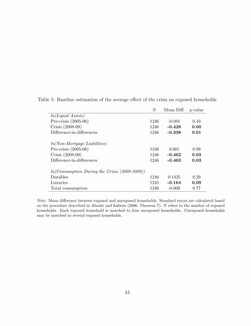
Table 5: Baseline estimation of the average effect of the crisis on exposed households
N Mean Diff. p-value
ln(Liquid Assets)Pre-crisis (2005-06) 1246 -0.091 0.43Crisis (2008-09) 1246 -0.428 0.00Difference-in-differences 1246 -0.338 0.01
ln(Non-Mortgage Liabilities)Pre-crisis (2005-06) 1246 0.001 0.99Crisis (2008-09) 1246 -0.462 0.03Difference-in-differences 1246 -0.463 0.03
ln(Consumption During the Crisis (2008-2009))Durables 1246 0.1425 0.29Luxuries 1245 -0.164 0.09Total consumption 1246 -0.009 0.77
Note: Mean difference between exposed and unexposed households. Standard errors are calculated basedon the procedure described in Abadie and Imbens (2006, Theorem 7). N refers to the number of exposedhouseholds. Each exposed household is matched to four unexposed households. Unexposed householdsmay be matched to several exposed households.
43

Tab
le6:
Est
imat
ion
ofth
eav
erag
eeff
ect
ofth
ecr
isis
onex
pos
edhou
sehol
ds
contr
olling
for
cred
itco
nst
rain
ts
Con
stra
ined
Un
con
stra
ined
NM
ean
diff
p-v
alu
eN
Mea
nd
iffp
-valu
e
ln(L
iqu
idA
sset
s)P
re-c
risi
s(2
005-0
6)
794
-0.0
090.
949
164
-0.3
13
0.124
Cri
sis
(2008-
09)
794
-0.305
0.056
164
-0.487
0.04
Diff
eren
ce-i
n-d
iffer
ence
s79
4-0.296
0.08
164
-0.1
730.4
92
ln(N
on
-Mort
gage
Lia
bili
ties
)P
re-c
risi
s(2
005-
06)
794
0.17
50.
542
164
0.1
19
0.788
Cri
sis
(200
8-0
9)
794
-0.734
0.01
164
0.678
0.1
48
Diff
eren
ce-i
n-d
iffer
ence
s79
4-0.909
0.001
164
0.559
0.2
62
ln(C
on
sum
pti
on
Du
rin
gth
eC
risi
s(2
008-2
009))
Du
rab
les
794
0.06
60.
695
164
-0.0
840.7
63
Lu
xu
ries
794
-0.0
660.
586
163
-0.0
490.7
75
Tot
al
con
sum
pti
on
794
0.02
0.61
9164
-0.0
140.8
24
Note
:M
ean
diff
eren
ceb
etw
een
exp
osed
an
du
nex
pose
dh
ou
seh
old
s.C
on
stra
ined
hou
seh
old
sare
defi
ned
as
hav
ing
at
least
20%
hom
eeq
uit
yan
dno
HE
LO
Cin
the
2005
-06
per
iod
(i.e
.,p
re-c
risi
s).
Un
const
rain
edh
ou
seh
old
sare
defi
ned
as
hav
ing
at
least
20%
hom
eeq
uit
yan
da
HE
LO
Cin
the
pre
-cri
sis
per
iod
.N
refe
rsto
the
nu
mb
erof
exp
ose
dh
ou
seh
old
sin
each
cate
gory
.S
tan
dard
erro
rsare
calc
ula
ted
bas
edon
the
pro
ced
ure
des
crib
edin
Ab
adie
an
dIm
ben
s(2
006,
Th
eore
m7).
44

Tab
le7:
Do
larg
eco
nsu
mpti
oneff
ects
imply
low
leve
lsof
liquid
asse
ts?
Bot
tom
Qu
arti
leof
Top
Thre
eQ
uart
iles
ofT
otal
Con
sum
pti
onA
TT
Tota
lC
onsu
mp
tion
AT
T
NM
ean
Std
.D
ev.
NM
ean
Std
.D
ev.
Mea
nD
iff.
AT
Ton
ln(T
ota
lC
on
sum
pti
on
)(C
risi
s)31
2-0
.974
0.49
293
30.
316
0.492
-1.2
91*
**A
TT
on
ln(D
ura
bles
)(C
risi
s)31
2-1
.662
3.27
293
30.7
47
2.923
-2.4
09**
*A
TT
on
ln(L
uxu
ries
)(C
risi
s)31
2-1
.486
2.39
493
30.2
79
2.07
-1.7
65*
**
AT
Ton
Ch
an
gein
ln(L
iqu
idA
sset
s)31
2-0
.437
3.25
893
3-0
.294
3.122
-0.1
42
AT
Ton
Ch
an
ge
inln
(Non
-Mort
gage
Lia
b.)
312
-0.5
145.
413
933
-0.4
494.
984
-0.0
64
ln(L
iqu
idA
sset
s)of
Exp
ose
dH
Hs
(Pre
-cri
sis)
312
7.72
42.
274
933
8.1
32
2.277
-0.4
09*
**ln
(Liq
uid
Ass
ets)
of
Exp
ose
dH
Hs
(Cri
sis)
312
7.56
12.
852
933
8.0
92
2.6
98
-0.5
31*
**
ln(N
on
-Mort
gage
Lia
b.)
ofE
xp
osed
HH
s(P
re-c
risi
s)31
25.
496
4.49
5933
6.385
4.547
-0.8
89**
*ln
(Non
-Mort
gage
Lia
b.)
ofE
xp
osed
HH
s(C
risi
s)31
25.
172
4.63
893
35.9
69
4.679
-0.7
97*
**
Note
:N
refe
rsto
the
nu
mb
erof
exp
osed
hou
seh
old
sin
each
cate
gory
(bott
om
qu
art
ile
vs.
the
top
thre
equ
art
iles
).***,
**
an
d*
ind
icate
sign
ifica
nce
atth
e1%
,5%
and
10%
level
s,re
spec
tive
ly.
45

Table 8: Baseline estimation of the average effect of the crisis on the imputed consumption ofexposed households
N Mean Diff. p-value
ln(Basic Imputed Consumption)Pre-crisis (2005-06) 532 -0.243 0.443Crisis (2008-09) 532 0.205 0.56Difference-in-differences 532 0.447 0.305
ln(Complete Imputed Consumption)Pre-crisis (2005-06) 532 -0.767 0.314Crisis (2008-09) 532 -0.722 0.309Difference-in-differences 532 0.045 0.964
Note: Mean difference between exposed and unexposed households. Standard errors are calculated basedon the procedure described in Abadie and Imbens (2006, Theorem 7). N refers to the number of exposedhouseholds. Each exposed household is matched to four unexposed households. Unexposed householdsmay be matched to several exposed households.
Table 9: Estimation of the average effect of the crisis on the imputed consumption of exposedhouseholds controlling for credit constraints
Constrained UnconstrainedN Mean diff p-value N Mean diff p-value
ln(Basic Imputed Consumption)Pre-crisis (2005-06) 373 -0.036 0.349 159 0.234 0.702Crisis (2008-09) 373 0.465 0.934 159 0.398 0.384Difference-in-differences 373 0.502 0.431 159 0.164 0.783
ln(Complete Imputed Consumption)Pre-crisis (2005-06) 373 -1.188 0.213 159 -0.952 0.872Crisis (2008-09) 373 -0.856 0.358 159 -0.256 0.872Difference-in-differences 373 0.332 0.799 159 0.696 0.701
Note: Mean difference between exposed and unexposed households. Constrained households are definedas having at least 20% home equity and no HELOC in the 2005-06 period (i.e., pre-crisis). Unconstrainedhouseholds are defined as having at least 20% home equity and a HELOC in the pre-crisis period. Nrefers to the number of exposed households in each category. Standard errors are calculated based on theprocedure described in Abadie and Imbens (2006, Theorem 7).
46

Table 10: Balance of household characteristics, using the wholesale funding-based Exposuremeasure (two-sample t-test)
Exposed Unexposed p-value
Home equity / house value 0.663 0.657 0.623ln(House value) 10.442 10.339 0.416ln(Gross income) 10.986 10.992 0.788Age 49.51 49.514 0.986Single 0.324 0.340 0.260Unemployed 0.030 0.028 0.787House size 4.694 4.631 0.327Labor supply, male 0.652 0.657 0.698Labor supply, female 0.554 0.549 0.711Self-employed, male 0.076 0.065 0.146Self-employed, female 0.084 0.083 0.851College some 0.167 0.164 0.762College degree 0.653 0.664 0.3841-2 children 0.246 0.238 0.4613-4 children 0.014 0.010 0.2465 children 0.002 0.001 0.327Big city 0.390 0.399 0.502Renter 0.166 0.175 0.376French 0.470 0.468 0.659Risk aversion 0.124 0.126 0.508
Observations 1658 1658
47
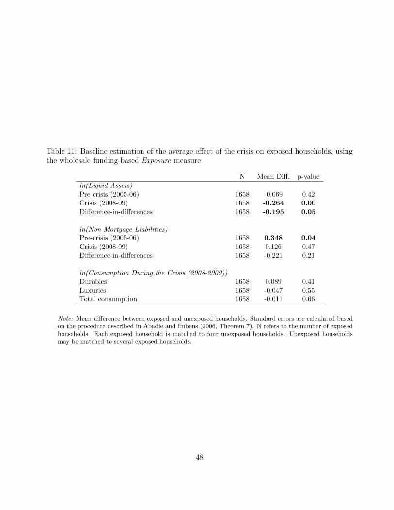
Table 11: Baseline estimation of the average effect of the crisis on exposed households, usingthe wholesale funding-based Exposure measure
N Mean Diff. p-value
ln(Liquid Assets)Pre-crisis (2005-06) 1658 -0.069 0.42Crisis (2008-09) 1658 -0.264 0.00Difference-in-differences 1658 -0.195 0.05
ln(Non-Mortgage Liabilities)Pre-crisis (2005-06) 1658 0.348 0.04Crisis (2008-09) 1658 0.126 0.47Difference-in-differences 1658 -0.221 0.21
ln(Consumption During the Crisis (2008-2009))Durables 1658 0.089 0.41Luxuries 1658 -0.047 0.55Total consumption 1658 -0.011 0.66
Note: Mean difference between exposed and unexposed households. Standard errors are calculated basedon the procedure described in Abadie and Imbens (2006, Theorem 7). N refers to the number of exposedhouseholds. Each exposed household is matched to four unexposed households. Unexposed householdsmay be matched to several exposed households.
48

Tab
le12
:D
ola
rge
consu
mpti
oneff
ects
imply
low
leve
lsof
liquid
asse
ts,
when
the
whol
esal
efu
ndin
g-bas
edE
xpos
ure
mea
sure
isuse
d?
Bot
tom
Qu
arti
leof
Top
Th
ree
Qu
art
iles
ofT
otal
Con
sum
pti
onA
TT
Tota
lC
onsu
mp
tion
AT
T
NM
ean
Std
.D
ev.
NM
ean
Std
.D
ev.
Mea
nD
iff.
AT
Ton
ln(T
ota
lC
on
sum
pti
on
)(C
risi
s)41
5-0
.950
0.48
6124
20.
305
0.4
66
-1.2
51*
**A
TT
on
ln(D
ura
bles
)(C
risi
s)41
5-1
.724
3.21
512
420.
695
2.942
-2.4
19**
*A
TT
on
ln(L
uxu
ries
)(C
risi
s)41
5-1
.567
2.68
3124
20.4
61
1.9
47
-2.0
28*
**
AT
Ton
Ch
an
ge
inln
(Liq
uid
Ass
ets)
415
-0.3
253.
085
1242
-0.1
45
2.969
-0.1
80
AT
Ton
Ch
an
ge
inln
(Non
-Mort
gage
Lia
b.)
415
-0.4
815.
017
1242
-0.1
33
5.234
-0.3
48
ln(L
iqu
idA
sset
s)of
Exp
ose
dH
Hs
(Pre
-cri
sis)
415
7.90
62.
080
124
28.
313
2.2
38
-0.4
07*
**ln
(Liq
uid
Ass
ets)
of
Exp
ose
dH
Hs
(Cri
sis)
415
7.83
72.
621
124
28.
466
2.3
49
-0.6
29*
**
ln(N
on
-Mort
gage
Lia
b.)
ofE
xp
osed
HH
s(P
re-c
risi
s)41
56.
359
4.31
1124
26.6
51
4.5
01
-0.2
92ln
(Non
-Mort
gage
Lia
b.)
ofE
xp
osed
HH
s(C
risi
s)41
55.
803
4.55
712
426.
286
4.704
-0.4
83*
Note
:N
refe
rsto
the
nu
mb
erof
exp
osed
hou
seh
old
sin
each
cate
gory
(bott
om
qu
art
ile
vs.
the
top
thre
equ
art
iles
).***,
**
an
d*
ind
icate
sign
ifica
nce
atth
e1%
,5%
and
10%
level
s,re
spec
tive
ly.
49


