37
Basic Concepts of Discrete Probability (Theory of Sets: Continuation) 1
| Date post: | 31-Dec-2015 |
| Category: |
Documents |
| Upload: | bartholomew-payne |
| View: | 221 times |
| Download: | 0 times |

Basic Concepts of Discrete Probability
(Theory of Sets: Continuation)
1

Functions
• If X is a set and Y is a set, and there is a sequence of well-specified operations for assigning a well-defined object to every element , and by applying these sequence of operations to every member of a set X we obtain a set Y, then this sequence of operations forms a rule, which is commonly known as function.
y Yx X
2
Functions
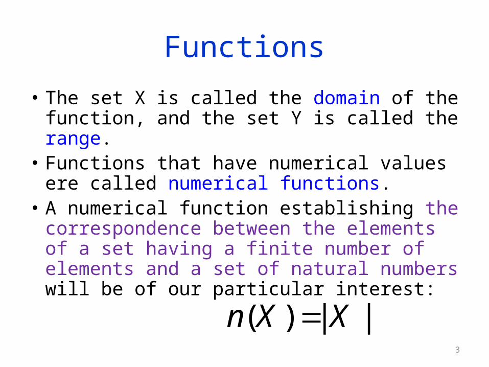
• The set X is called the domain of the function, and the set Y is called the range.
• Functions that have numerical values ere called numerical functions.
• A numerical function establishing the correspondence between the elements of a set having a finite number of elements and a set of natural numbers will be of our particular interest:
( ) | |n X X3

The number of elements in a set
• The number of elements in a set may or may not be finite.
• If the elements of the set can be placed in one-to-one correspondence with the set of natural numbers {1, 2, 3,…}, we say that the set has a denumerable or countable number of elements; otherwise the set is nondenumerable (e.g., a set of points on any line or the set of points in [0,1]).
4

The number of elements in a set
• If a set is denumerable and is a finite number, we say that the power of the set X (the cardinality of the set X) is |X| (the number of elements in the set X).
• If a set is equivalent to the set of points in [0,1] that is, it is denumerable, we say that the set has the power of continuum.
( ) | |n X X
5

The number of elements in a set• The following properties hold for finite sets::• If A and B are two disjoint sets, then
• For any finite sets A, B, and C:
( ) ( ) ( )n A B n A n B
( ) ( ) ( ) ( )
( ) ( ) ( )
( ) ( )
( )
( )
( )
( ) ( ) ( )
( ) ( ) ( ) ( ) ( ) ( ) ( )
( ) ( ) ( ) ( ) ( ) ( )ABC
n A B n A n B n AB
n A B n A n AB
n A n A n U
n A B C n A n B C n AB AC
n A n B n C n BC n AB n AC n ABA
n A B C
n A n B n C n BC n AB n AC n AB
C
C
6
Basic Concepts of Discrete Probability
Elements of the Probability Theory
7

Sample Space
• When “probability” is applied to something, we usually mean an experiment with certain outcomes.
• An outcome is any one of the possibilities that may be expected from the experiment.
• The totality of all these outcomes forms a universal set which is called the sample space.
8

Sample Space
• For example, if we checked occasionally the number of people in this classroom on Tuesday from 7pm to 9-45pm, we should consider this an experiment having 15 possible outcomes {0,1,2,…,13,14} that form a universal set.
• 0 – nobody is in the classroom, … 14 – all students taking the Information Theory Class and the instructor are in the classroom
9

Sample Space
• A sample space containing at most a denumerable number of elements is called discrete.
• A sample space containing a nondenumerable number of elements is called continuous.
10

Sample Space
• A subset of a sample space containing any number of elements (outcomes) is called an event.
• Null event is an empty subset. It represents an event that is impossible.
• An event containing all sample points is an event that is certain to occur.
11

Probability Measure
• The probability measure is a specific type of function which can be associated with sets.
• Since an experiment is defined so that to each possible outcome of this experiment there corresponds a point in the sample space, the number of outcomes of the experiment is assumed to be at most denumerable.
12

Probability Measure• Let us consider an event of interest A as the set of
outcomes ak.
• Let a real function m(ak ) be the probability measure of the outcome ak.
• The probability measure of an event is defined as the sum of the probability measures associated with all the outcomes ak of that event. It is also referred to as the “additive probability measure”:
131
{ } ( )n
kk
m A m a

Probability Measure
• The additive probability measure has the following important property: the measure associated with the union of two disjoint sets is equal to the sum of their individual measures.
14

Probability Measure
• Two events A and B are called disjoint if they contain no outcome in common: two disjoint events cannot happen simultaneously. The probability measure has the following assumed properties:
15
0
{ } { } if and are disjoint
{ } 0 if
{ } 1 if
km a
m A B m A m B A B
m X X
m X X U

Probability Measure
• If with an additive probability measure, then the following relations are valid:
16
, ,A U B U C U
{ } { } if
{ } { } { }
{ } { } { } { } 1 { }
( ) { } { } { }
{ }
{ } { } {
{ } { } { }
}A B
m A m BA B
m A m B m B A
m A m U A m U m A m A
m A AB B m A m AB m Bm A B
m A m B m AB
m A m B m AB

Probability Measure
• For three disjoint sets :
• For three sets in general:
17
, ,A U B U C U
{ } { } { } { }m A B C m A m B m C
{ } { } { } { }
{ } { } { } { }
m A B C m A m B m C
m AB m BC m CA m ABC

Frequency of events
• Let us consider a specific event Xk among all the possible events of the experiment under consideration. If the basic experiment is repeated N times among which the event Xk has appeared times, the ratio
is defined as the relative frequency of the occurrence of the event Xk.
18
kn X
/kn X N

Frequency of events. The Probability
• If N is increased indefinitely, that is if then, intuitively speaking,
is the probability of the event Xk.
19
N
limN
kkn X
XN
P

The Probability
• The classical definition of Laplace says that the probability is the ratio of the number of favorable events to the total number of possible events.
• All events in this definition are considered to be equally likely: e.g., throwing of a true die by an honest person under prescribed circumstances…
• …but not checking of the number of people in the classroom.
20

The Probability
• The following properties are important:
21
0
0 1
0 lim 1
0 1
k
k
N
k
k
n X N
P
X
N
NX
n
n X

The Probability
• To verify whether our “empiric” definition of probability satisfies the properties of the probability measure, we have to consider the probability of two events.
• Let A and B be the events among the ones resulting from the experiment. Let the experiment be repeated n times.
22

The Probability
• Each observation can belong to only one of the four following categories:
• 1) A has occurred, but not B AB’;• 2) B has occurred, but not A BA’;• 3) Both A and B have occurred AB;
• 4) Neither A nor B has occurred A’B’
23
'A AB AB
'B BA AB
' 'A B AB AB BA

The Probability• If the number of events of each category from the
mentioned four ones is denoted by then
• relative frequency of A
independent of B
• relative frequency of B independent of A
24
1 2 3 4, , ,n n n n
1 2 3 4n n n n n
1 3n nf A
n
2 3n nf A
n

The Probability
• relative frequency of either A, B or both
• relative frequency of A and B occurring together
• relative frequency of A under condition that B has occurred
• relative frequency of B under condition that A has occurred
25
1 2 3n n nf A B
n
3nf AB
n
3
2 3
|n
f A Bn n
3
1 3
|n
f B An n
The Probability
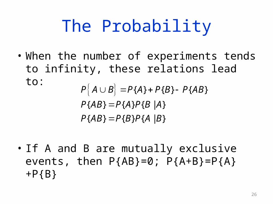
• When the number of experiments tends to infinity, these relations lead to:
• If A and B are mutually exclusive events, then P{AB}=0; P{A+B}=P{A}+P{B}
26
{ } { } { }
{ } { } { | }
{ } { } { | }
P A B P A P B P AB
P AB P A P B A
P AB P B P A B

The Probability• Thus, we have proved that
• Let us compare the latter with the properties of the probability measure:
27
0 1
{ } { } for mutually exclusive and
{ } 0 if, and only if,
{ } 1 if, and only if,
P A
P A B P A P B A B
P X X
P X X U
0
{ } { } if and are disjoint
{ } 0 if
{ } 1 if
km a
m A B m A m B A B
m X X
m X X U

The Probability
• We have just shown that our empirical definitions of the frequency and probability, respectively, satisfy all the properties of the probability measure.
28

Theorem of addition
• For two events A and B of the sample space:
• The additive property of the probability measure suggests that
• If A and B are mutually exclusive events, then
29
( )A B AB A B
{ } { } { } { }
{ } { } { } { } { } { }
m A B m A m B m AB
P A B P A P B P AB P A P B
{ } { } 0
{ } { }
P AB P
P A B P A P B
Theorem of addition
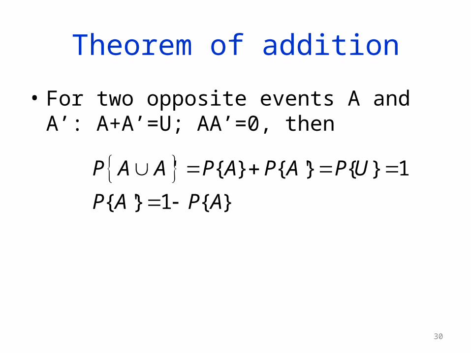
• For two opposite events A and A’: A+A’=U; AA’=0, then
30
' { } { '} { } 1
{ '} 1 { }
P A A P A P A P U
P A P A

Theorem of addition
• For the three events A, B, and C:
• In general, for a number of events
31
{ } ( )
{ } { } { } { } { } { } } {
P A B C
P A P B
P A B P C P A B
P C P AB P BC P CA P B
C
A C
1 2, ,..., nA A A
1 2 1 2
1 2 1 3 1 1 2 3 1 2 4
12 1 1 2
... ...
...
... ... ( 1) ...
n n
n n
nn n n n
P A A A P A P A P A
P A A P A A P A A P A A A P A A A
P A A A P A A A

Theorem of addition
• If the events are mutually exclusive, then
• It is also clear now that
32
1 2 1 2... ...n nP A A A P A P A P A
1 2 1 2... ...n nP A A A P A P A P A
Conditional Probability
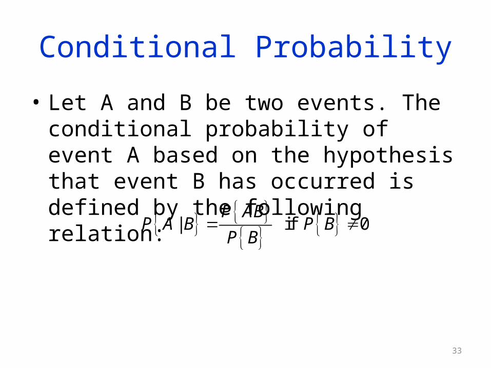
• Let A and B be two events. The conditional probability of event A based on the hypothesis that event B has occurred is defined by the following relation:
33
| if 0
P ABP A B P B
P B

Conditional Probability
• Returning to the example of two events• 1) A has occurred, but not B AB’ n1;
• 2) B has occurred, but not A BA’ n2;
• 3) Both A and B have occurred AB n3;
• 4) Neither A nor B has occurred A’B’ n4:
34
3
2 3
3
1 3
| ;
|
f ABnf A B
n n f B
f ABnf B A
n n f A

Conditional Probability
• The two events A and B are called mutually independent if P{A|B}=P{A} and P{B|A}=P{B}.
• For mutually independent events P{AB}=P{A}P{B}.
35

Theorem of multiplication
• The multiplication rule for the case of two events A and B can be obtained through the definition of the conditional probability: P{AB}=P{A}P{B|A}=P{B}P{A|B}.
• For three events A,B, and C: P{ABC}=P{AB}P{C|AB}=P{A}P{B|A}P{C|AB}
36

Theorem of multiplication
• For n events:
• For a countable infinite number of the mutually independent events
37
1 2
1 2 1 3 1 2 1 2 1
...
{ } { | } | ... { | ... }
n
n n
P A A A
P A P A A P A A A P A A A A
1 2 1 2... { } { }... { }n nP A A A P A P A P A


