30
Basics in Process Design Frej Bjondahl 2006

Basics in Process Design
Frej Bjondahl
2006

2
Contents Basics in Process Design ...............................................................................................1 Contents .........................................................................................................................2 1. Introduction............................................................................................................3 2. Design/analysis of process systems using mass and energy balances ...................3
2.1 Balance boundary, input, output, recirculation ..............................................4 2.2 Batch, continuous, steady state, dynamic process .........................................5 2.3 Mixing, chemical reaction, separation, recirculation, accumulation .............6 2.4 Heating, cooling, heat of reaction, phase change, pressure change ...............7
2.4.1 Example – mass balances.......................................................................7 2.4.2 Example – energy balances....................................................................8
3. Transport systems for of fluids ..............................................................................9 3.1 Pressure loss in piping, pipe element resistance ............................................9 3.2 Local pressure in pipe systems ....................................................................13 3.3 Pipe system characteristic curve ..................................................................13 3.4 Pump types, centrifugal, displacement ........................................................14 3.5 Pump characteristic, work point, power, efficiency, recalculation models .14 3.6 Pump and pipe systems, flow control ..........................................................16
3.6.1 Example pipe system ...........................................................................18 3.6.2 Example pipe and pump system ..........................................................19
3.7 Gas transport with fans in ducts...................................................................21 3.8 Gas transport with compressors ...................................................................21 3.9 Compressor types, centrifugal, displacement ..............................................21 3.10 Compressor calculations ..............................................................................21
3.10.1 Example – compressors .......................................................................24 3.11 Typical flow velocities.................................................................................24
4. Heat exchanger systems.......................................................................................25 4.1 Heat exchanger types ...................................................................................25 4.2 Heat exchanger modeling, counter current, co-current, real world .............25 4.3 Overall heat transfer coefficient...................................................................27 4.4 Condensing steam, evaporation ...................................................................27 4.5 Heat exchanger networks, pinch analysis ....................................................27
4.5.1 Example ...............................................................................................28 5. Economic analysis – modeling and selection ......................................................30

3
1. Introduction This course deals with some of the tools you can use for analysis and design of proc-ess systems as well as modeling of some basic and essential components or units used in such designs. The important part in process design is the system, not its individual units.
The vocabulary used in process design is also good to know and important words or phrases are therefore highlighted in the text using italic.
Process design often involves large systems. These will have to be broken down into smaller parts in order to be able to model and analyze these parts both individually and together with the entire system. Information and knowledge from many sources are combined and during the design you generally move from an overall view or goal into ever increasing detail until you have managed to create a complete process de-sign.
2. Design/analysis of process systems using mass and energy balances
Consider this process design problem – you have been asked to design a process for the production of a certain amount of product. Your task is to find out how to produce the product and then to design a process for the production.
First you find out what it is that you are supposed to do. You find out from your em-ployer/customer what they expect from the process.
Using literature, by making experiments and so on you find out what is needed to ac-complish the process. You can gather information about possible raw materials, nec-essary raw materials processing, what reactions are taking place, what kind of mixing and separation equipment can be used, the conditions in the process like required temperatures and pressures in each step, possibilities/necessity for recirculation of un-reacted raw material, generated waste or byproducts as well as properties for each ma-terial that goes through the process, and so on.
Once you have found out what kind of process steps are needed and what the condi-tions in the process steps should be you have to decide how large each piece of equipment should be and/or how much raw material, utilities and energy is needed. A basic tool you can use for this step in the design is the mass- and energy balance. Once you know the mass flows and energy requirements you can select equipment of suitable sizes for your process. You can also estimate what the process will cost to build and operate.
Mass and energy balances can also be used for analysis of processes – you have an existing process and want to analyze it in some way. You might want to study what happens if you make changes in the process. Mass and energy balances can be used to determine the accuracy of measurements, determine missing pieces of information or to determine where to make additional measurements.

4
2.1 Balance boundary, input, output, recirculation The first thing you need to do in order to make a mass and energy balance is to decide where the boundary for the balance is.
You can place the boundary anywhere but some ways of choosing makes it easier to use the balance.
Let us consider a process where the raw materials A and B are mixed and react ac-cording to
CB2A ↔+
Assuming that the reaction is not complete, some of the raw material remains unre-acted and it is separated from the product C. The unreacted raw material is recircu-lated back to the beginning of the process.
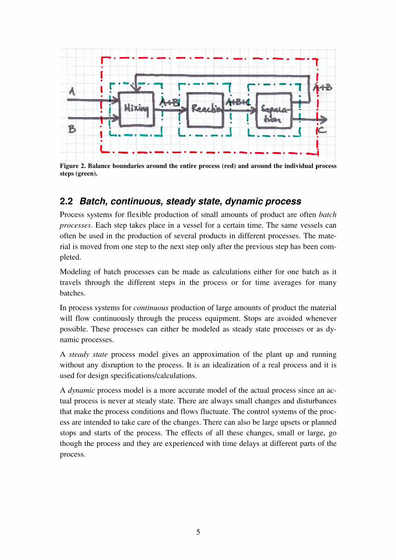
In order to visualize the process you can draw a simple block flow diagram (see Figure 1) that shows the material flows and the process steps. You can also give names (or numbers) to the flows and the process steps and write known or given data regarding the flows or the process conditions in the diagram.
Figure 1. Block flow diagram of a simple process. The three major process steps have been named Mixing, Reaction, and Separation. The flows have not been named but the components in each flow have been listed.
Some possible ways of choosing balance boundaries for the process in Figure 1 are shown in Figure 2. These are
a) an overall balance boundary around the entire process (including the recircu-lation)
b) balance boundaries around each process step (Mixing, Reaction, Separation)
c) partial mass balances for components A, B or C using the same balances boundaries as in a) and b)
Sometimes you only need one balance to find out what you need while at other times you might need all these balances as well as additional information. The additional information needed can be the stoichiometry of the chemical reaction, limiting condi-tions for the reaction, the extent of reaction, the separation efficiency, the recirculation ratio and so on. The solution can be found by solving a single equation or by solving a system of many equations either algebraically or numerically.
5
Figure 2. Balance boundaries around the entire process (red) and around the individual process steps (green).
2.2 Batch, continuous, steady state, dynamic process Process systems for flexible production of small amounts of product are often batch processes. Each step takes place in a vessel for a certain time. The same vessels can often be used in the production of several products in different processes. The mate-rial is moved from one step to the next step only after the previous step has been com-pleted.
Modeling of batch processes can be made as calculations either for one batch as it travels through the different steps in the process or for time averages for many batches.
In process systems for continuous production of large amounts of product the material will flow continuously through the process equipment. Stops are avoided whenever possible. These processes can either be modeled as steady state processes or as dy-namic processes.
A steady state process model gives an approximation of the plant up and running without any disruption to the process. It is an idealization of a real process and it is used for design specifications/calculations.
A dynamic process model is a more accurate model of the actual process since an ac-tual process is never at steady state. There are always small changes and disturbances that make the process conditions and flows fluctuate. The control systems of the proc-ess are intended to take care of the changes. There can also be large upsets or planned stops and starts of the process. The effects of all these changes, small or large, go though the process and they are experienced with time delays at different parts of the process.

6
2.3 Mixing, chemical reaction, separation, recirculation, ac-cumulation
Mixing, chemical reaction and separation are some of the most basic steps in a chemical engineering process that must be taken into account in mass and energy bal-ances.
The mass balance model for mixing is easy if you assume that no reaction takes place. All components that enter the mixer come out again. The energy balance might be more difficult since the flows into the mixer can be of different composition, pressure, temperature and phase. The modeling becomes more difficult if some kind of reac-tion, dissolution or change of phase takes place during mixing.
In the reaction step you take into account that some components react and disappear producing other components. The reaction stoichiometry is used to keep track of the balance between reactants and products. The total mass flow out is the same as the flow in if you assume steady-state conditions. The extent of reaction (or conversion) needed for partial mass balances is more difficult to model since it also depends on the process conditions (like residence time in the reactor, concentration of reactants and products, pressure, temperature, presence of catalysts, mixing, particle sizes and so on). The raw material flows, the heat of reaction, reactor heating/cooling all affect the energy balance.
Modeling of the separation step is also difficult since the separation efficiency de-pends on the choice of separation method and the conditions in the process step. Sepa-ration is rarely perfect, you almost always loose raw materials in the product flow and you separate and throw away/recirculate product. Splitting, distillation, filtering, crys-tallization, chromatography, stripping, flashing are all examples of separation meth-ods.
Recirculation of material in the process does not make the mass and energy balance modeling more difficult but it can make the calculations more difficult. You quite of-ten need to make iterative numerical calculations to reach a result. When recirculation is used you also recirculate impurities that can accumulate in process. In order to keep the concentration of these impurities low you might have to purge some of the recir-culated material as waste.
Usually you assume that the process is in steady state i.e. that no accumulation takes place in the process steps (at least in the long run). Sometimes accumulation takes place anyway and you have to take that into account. This is especially true when you model existing processes using measured data.
The mass balance calculations require that you can convert material flows given as mass, mol and volume between each other depending on the models used. The com-position of the flows might be given as concentration as well mass, mol and volume ratio depending on the circumstances when different reaction and separation models are used together with the mass balance models.

7
2.4 Heating, cooling, heat of reaction, phase change, pres-sure change
The material flows might also have to be heated or cooled. You might want to start or stop chemical reactions or change the physical or transport properties of the flows. The reactions taking place might require heat or produce heat depending on the reac-tion. The process might give off or take up heat from the surroundings.
The reactions, separation or the transport might also cause or require changes in pres-sure using pumps, fans, compressors, valves and flashes. All these steps or phenom-ena affect the energy flows in the process and they are be accounted for in the energy balances.
You must be able to use thermodynamic models for calculation of enthalpy of com-pounds, enthalpy of reaction, enthalpy of evaporation, enthalpy of dissolution, en-thalpy of mixtures, and so on when you calculate the energy flows with the materials and the necessary external energy flows needed to accomplish changes in these. En-ergy can also be recirculated within the process when warm flows need cooling and cold flows need heating.
2.4.1 Example – mass balances In a factory the production rate of ammonia is 1000 kg/h. Ammonia (NH3) can be pro-duced from hydrogen gas (H2) and nitrogen gas (N2) using the Haber-Bosch process.
(g)2NH(g)H3(g)N 322 ↔+
The molar mass of nitrogen gas is 28.01 kg/kmol, the molar mass of hydrogen gas is 2.02 kg/kmol, and the molar mass of ammonia is 17.03 kg/kmol. The conversion of nitrogen in the reactor (here defined as mol nitrogen gas reacted)/(mol nitrogen gas in) is assumed to be about 17 %. Unreacted hydrogen and nitrogen is separated and recir-culated to the reactor.
a) How large are the flows in this process?
b) What is the composition of the flows?
The block flow diagram below shows the main steps in the process.
Mixer
Reactor
Separator
1
2 3
6
4 5
8
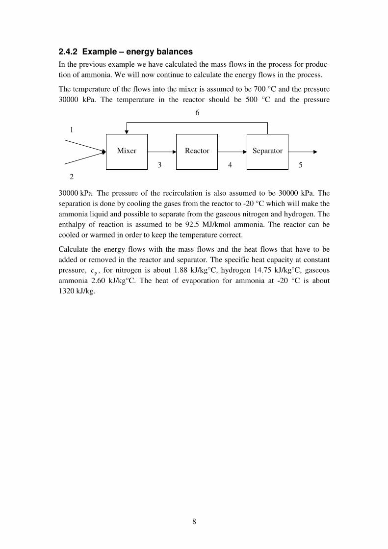
2.4.2 Example – energy balances In the previous example we have calculated the mass flows in the process for produc-tion of ammonia. We will now continue to calculate the energy flows in the process.
The temperature of the flows into the mixer is assumed to be 700 °C and the pressure 30000 kPa. The temperature in the reactor should be 500 °C and the pressure
30000 kPa. The pressure of the recirculation is also assumed to be 30000 kPa. The separation is done by cooling the gases from the reactor to -20 °C which will make the ammonia liquid and possible to separate from the gaseous nitrogen and hydrogen. The enthalpy of reaction is assumed to be 92.5 MJ/kmol ammonia. The reactor can be cooled or warmed in order to keep the temperature correct.
Calculate the energy flows with the mass flows and the heat flows that have to be added or removed in the reactor and separator. The specific heat capacity at constant pressure, pc , for nitrogen is about 1.88 kJ/kg°C, hydrogen 14.75 kJ/kg°C, gaseous ammonia 2.60 kJ/kg°C. The heat of evaporation for ammonia at -20 °C is about 1320 kJ/kg.
Mixer
Reactor
Separator
1
2 3
6
4 5
9
3. Transport systems for of fluids The processes in a chemical plant involve a lot of process steps and in particular trans-port of material between these steps. Sometimes the transport systems are also respon-sible for changing the pressure of the materials in the process. The design of these transport systems is a large part of the design of process systems.
The mass balances give the sizes of the flows in different parts of the system. The conditions required in the different parts of the system gives information for the calcu-lation of the transport properties of the material flows.
3.1 Pressure loss in piping, pipe element resistance When liquids or gases flow through pipes they experience a resistance due to wall friction which slows down the flow. There is also additional resistance in the parts of the pipe system where the flow has to change direction or velocity like in pipe bends, valves and other pipe fittings. The resistance causes energy in the form of pressure to become heat and this is experienced and measured as a pressure loss in the pipe sys-tem as the fluid flows through it.
It is possible to model the resistance in pipe systems or parts of pipe systems. You can calculate the total pressure loss in the system when a certain volume flow flows through the system. You can calculate the local pressure at any point in the pipe sys-tem. The volume flow (velocity) together with inlet and outlet pressure, inlet and out-let height, fluid density and viscosity as well as any phase change determine the pres-sure at any point in the system given the configuration of the system. Pumps (for liq-uids) and fans (for gases) are used when the pressure has to be increased while valves are used when the pressure has to be decreased to reach a certain flow.
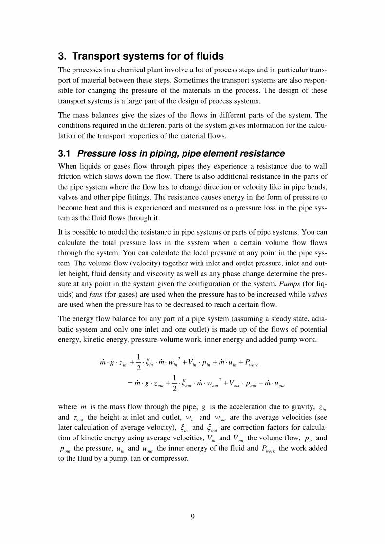
The energy flow balance for any part of a pipe system (assuming a steady state, adia-batic system and only one inlet and one outlet) is made up of the flows of potential energy, kinetic energy, pressure-volume work, inner energy and added pump work.
outoutoutoutoutout
workinininininin
umpVwmzgm
PumpVwmzgm
⋅+⋅+⋅⋅⋅+⋅⋅=
+⋅+⋅+⋅⋅⋅+⋅⋅
��������
2
2
21
21.
ξ
ξ
where m� is the mass flow through the pipe, g is the acceleration due to gravity, inz
and outz the height at inlet and outlet, inw and outw are the average velocities (see later calculation of average velocity), inξ and outξ are correction factors for calcula-tion of kinetic energy using average velocities, inV
� and outV
� the volume flow, inp and
outp the pressure, inu and outu the inner energy of the fluid and workP the work added to the fluid by a pump, fan or compressor.

10
For liquids (and also for gases at moderate pressure changes) the density does not change much due to change in pressure and the volume flow in and out will be almost the same. The equation can the be rearranged into
( ) ( ) ( ) ( )22
21
ininoutoutinoutworkoutinoutin wwmuumPzzgmppV ⋅−⋅⋅⋅+−⋅=+−⋅⋅+−⋅ ξξ����
The pump work is added to the energy flow as pressure-volume work
VpP pumpwork
�⋅∆=
The power that is actually provided to the pump depends on the pump efficiency
pump
workpump
PP
η=
The change in inner energy is due to friction and the friction causes the fluid that is being pumped to heat up. This change is almost linearly proportional to the kinetic energy of the flow and it is usually modeled using friction factors according to
( )�
⋅⋅⋅≡−⋅ ζ2
21 wmuum inout ��
where � ζ is the sum of friction factors in this part of the pipe system. Division of the energy flow balance by the volume flow (possible only if the density is close to constant as it is for liquids but also for gases at moderate pressure change) makes it possible to express the energy balance using pressure
( ) ( ) ( )222
21
21
ininoutoutpumpoutinoutin wwwpzzgpp ⋅−⋅⋅⋅+⋅⋅⋅=∆+−⋅⋅+− ξξρζρρ
If the pipe has the same inlet and outlet velocity (i.e. the same density and pipe diame-ter) then the kinetic energy in and out is the same and the equation can be simplified into
( ) ( ) ⋅⋅⋅=∆+−⋅⋅+− ζρρ 2
21 wpzzgpp pumpoutinoutin
The average velocity can be calculated using the volume flow and the cross section area of the pipe.
AVw �=

11
The sum of friction factors is made up of the sum of the friction factors for different pipe elements and the wall friction which also depends on the length and diameter of the pipe
��⋅+= delements d
l ζζζ
The flow resistance depends on the roughness of the pipe and it can be estimated us-ing
25.0094.16 10007.181001.0 ������ ������ ⋅⋅+⋅=
dk
Redζ
where Re is the Reynolds number and k is the surface roughness. The Reynolds number can be calculated as
ηρ
ν⋅⋅=⋅= dwdwRe
where w is the flow velocity, d is the diameter, ν is the cinematic viscosity, ρ is the density and η is the dynamic viscosity. The flow is considered to be laminar if the Reynolds number is below 2300 (the correction factor ξ is then about 2). Above that the flow is usually turbulent (and ξ is about 1.1). Table 1. Surface roughness for some common surface types. Most clean pipes have very low sur-face roughness while the surface roughness of dirty or corroded pipes can be up to a 100 times larger.
Type of surface Surface roughness, k
Smooth pipe 0.02 – 0.05 mm
Galvanized pipe 0.1 – 0.2 mm
Smooth cement 0.2 – 0.5 mm
Rusted iron, concrete 1 – 2 mm
If a pipe or duct is not circular (square, rectangular or any other shape) then the hy-draulic diameter can be used instead of the diameter. It is defined as
ph l
Ad ⋅= 4
where A is the cross section area of the pipe or duct and pl is the circumference of the pipe or duct.
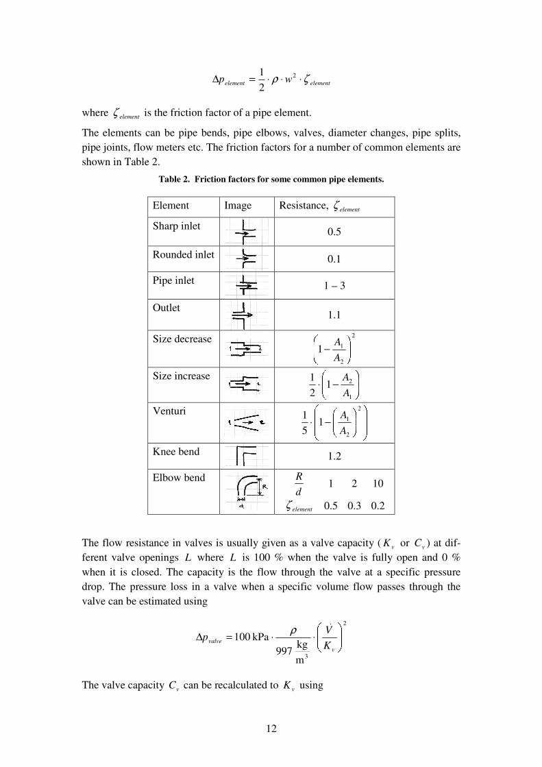
The pressure loss in any single element in the pipe can be modeled as
12
elementelement wp ζρ ⋅⋅⋅=∆ 2
21
where elementζ is the friction factor of a pipe element.
The elements can be pipe bends, pipe elbows, valves, diameter changes, pipe splits, pipe joints, flow meters etc. The friction factors for a number of common elements are shown in Table 2.
Table 2. Friction factors for some common pipe elements.
Element Image Resistance, elementζ
Sharp inlet
0.5
Rounded inlet
0.1
Pipe inlet
1 – 3
Outlet
1.1
Size decrease
2
2
11 �������� −AA
Size increase �� !""#$ −⋅
1
2121
AA
Venturi
%%&'(()
*%%&'(()*−⋅2
2
1151
AA
Knee bend
1.2
Elbow bend
dR 1 2 10
elementζ 0.5 0.3 0.2
The flow resistance in valves is usually given as a valve capacity ( vK or vC ) at dif-ferent valve openings L where L is 100 % when the valve is fully open and 0 % when it is closed. The capacity is the flow through the valve at a specific pressure drop. The pressure loss in a valve when a specific volume flow passes through the valve can be estimated using
2
3mkg 997
kPa 100 ++,-../0⋅⋅=∆v
valve KVp 1ρ
The valve capacity vC can be recalculated to vK using

13
234567⋅≈
234567Gal/min US
866.0/hm3
vv CK
3.2 Local pressure in pipe systems Given an inlet pressure and a flow into a pipe section you can calculate the pressure at the end of the section and use that as the inlet pressure in the following pipe section and thus calculate the pressure at any point in the pipe.
119
120
121
122
123
124
125
126
127
128
129
0 2 4 6 8 10 12pipe length from inle t (m)
pres
sure
(kPa
)
Figure 3. The curve shows the pressure at different positions along the length of the pipe system shown to the left. The pipe system has been divided into sections (numbered 1 to 7) and the pres-sure out from each section has been calculated using the inlet pressure to the section and the vol-ume flow through the pipe system.
If you know the inlet and outlet pressure but not the flow you can use an iterative method to find the flow that settles in the system due to gravity and differences in pressure at inlet and outlet.
1. Guess a volume flow through the system.
2. Calculate the pressure change in each section. The outlet pressure from each section is the inlet pressure (= outlet pressure from previous section) plus the change in pressure in the section. When you reach the outlet you have an out-let pressure.
3. If the outlet pressure is higher than the expected pressure, increase the volume flow and recalculate, if the outlet pressure is lower, reduce the volume flow and recalculate. The pressure drop is a quadratic function of the velocity (vol-ume flow). This means that if you calculate the pressure drop for three differ-ent flows you can use a second order polynomial for interpola-tion/extrapolation between pressure difference and volume flow.
4. When the calculated outlet pressure is the same as the expected outlet pressure you have found the volume flow that will develop in the system.
3.3 Pipe system characteristic curve You can calculate the total pressure loss in the pipe for different flows through the pipe and draw a pipe characteristic curve of this. An increase in flow causes more

14
friction and larger pressure losses in the system and the curve shows how much the pressure in the system must be increased (or decreased) in order to reach a certain volume flow through the system. This characteristic curve can be used together with similar curves for pumps and fans when choosing pumping equipment.
y = 0.0076x2 + 0.0074x - 8.3504
-20
0
20
40
60
80
100
120
140
160
180
0 20 40 60 80 100 120 140 160
volume flow (m3/h)
tota
l pre
ssur
e lo
ss (k
Pa)
Figure 4. The characteristic curve for the pipe system above that shows the total pressure loss as a function of the volume flow through the pipe system. A second order polynomial has been drawn through the calculated points and the equation for this curve is given in the graph.
3.4 Pump types, centrifugal, displacement Pumps are used in pipe systems to increase the pressure and the flow of liquids.
Common pumps are usually divided into two major types – centrifugal pumps and displacement pumps. Centrifugal pumps accelerate the pumped fluid using open im-pellers and then transform the kinetic energy (velocity) to pressure in diffusers. In displacement pumps the fluid is enclosed into compartments and moved from the low pressure side to the high pressure side.
3.5 Pump characteristic, work point, power, efficiency, recal-culation models
A pump that works at a certain speed (ω ) with a liquid of a certain density ( ρ ) can increase the pressure of that liquid a certain amount ( p∆ ) when it pumps a certain volume flow (V8 ) of the liquid.
The flow in a displacement pump depends almost only on the pump speed regardless of the increase in pressure. It does so since each volume of liquid is closed in a com-partment and moved (displaced) from the low pressure side to the high pressure side.
The flow in a centrifugal pump depends on the increase in pressure. The higher the pressure increase is the lower the volume flow. The liquid in the pump is never in a closed volume since the pump is open from inlet to outlet. The liquid is accelerated and the velocity is then transformed into pressure by changing the flow cross section area.

15
A pump characteristic curve can be created for any pump where the increase in pres-sure generated by the pump is plotted against the volume flow through the pump. The curve is valid only when the pump pumps a certain liquid at a certain speed.
A similar power characteristic curve can also be created which shows the power the pump needs at a certain volume flow (and pressure increase). Both types of curves are shown in Figure 5.
0
10
20
30
40
50
60
0 2 4 6 8 10 12 14 16
Volume flow (m3/h)
Pres
sure
incr
ease
(kPa
)
0
0.5
1
1.5
2
2.5
3
Pow
er (k
W)
Pressure increase Power
Figure 5. Pump and power characteristic curves for a centrifugal pump. The characteristic curves are defined for a certain pump, at a certain speed and using a certain liquid. To generate pump characteristics for each pump for any speed and any liquid is not very practical. Instead the pump manufacturers provide characteristic curves for pumps at a certain speed (like 1450 rpm) when they pump a certain liquid (like water with a density of 1000 kg/m3). Using these characteristic curves it is then possible estimate the pump characteristic curves for other pump speeds and liquids.
The coordinates in the pump characteristic curves can be recalculated to other liquid densities and pump speeds using
originaloriginal
new
original
new
original
newnew p
ddp ∆⋅99:
;<<=>⋅99:;<<=>⋅99:
;<<=>≈∆ρρ
ωω
22
originaloriginal
new
original
new
original
newnew P
ddP ⋅??@
ABBCD⋅??@ABBCD⋅??@
ABBCD≈ρ
ρωω
53
originaloriginal
new
original
newnew V
ddV EE ⋅FFG
HIIJK⋅FFGHIIJK≈
3
ωω
Note that all three ( p∆ , P and VL ) change at the same time!
The capacity of a pump can also be changed by changing the impeller diameter d (the moving part of a centrifugal pump is called an impeller). The equations above

16
show how a change in impeller diameter changes the characteristic curves of the pump.
Only a part of the power delivered to the pump is used for pressure-volume work. The remainder of the power becomes heat. The connection between power delivered and power used for pressure-volume work is given by the pump efficiency, η , which is defined as
PpV ∆⋅= Mη
The efficiency depends on the volume flow just as the pressure increase and the power and a corresponding efficiency characteristic curve can be drawn.
3.6 Pump and pipe systems, flow control The pump characteristic curve can be drawn in the same graph as the characteristic curve for the pipe system in which the pump is installed. The point where the two curves intersect gives the work point, i.e. the conditions that develop with this combi-nation of pump and system, see Figure 6.
-20
0
20
40
60
80
100
0 2 4 6 8 10 12 14 16
Volume flow (m3/h)
Pres
sure
incr
ease
(kPa
)
Pump Pipe system
Work point
Figure 6. The point where the pump characteristic curve and the pipe system curve cross each other is the work point for this combination of system and pump.
The position of the work point (i.e. the flow and pressure in the system) can be changed (controlled) either by changing something in the pipe system (opening and closing of valves, changing pipe size) or by changing something regarding the pump (pump model and size, pump type, pump speed).
Consider the pipe and pump system described in Figure 6. Decide how to accomplish the flows given below and calculate new graphs for these cases.
a) You want to increase the flow to 12 m3/h.
b) You want to decrease the flow to 7 m3/h.

17
In order to increase the flow through the system by changing the pipe system you would have to increase the pipe diameter and perhaps change or remove the valve. Recalculate the pressure loss at different volume flows in the pipe system using the new pipe diameters and/or valve resistances. Find the work points and check if the diameter or valve resistance must be increased or decreased.
-20
0
20
40
60
80
100
0 2 4 6 8 10 12 14 16
Volume flow (m3/h)
Pres
sure
incr
ease
(kPa
)
Pump Valve removed Pipe system
New work point
In order to change the flow through the system by changing the pump you might change the pump to a bigger or smaller one or change the speed of the existing pump. Data for other pumps can be found from data given by the pump manufacturers.
If the speed is changed then the coordinates in the pump characteristic curve (volume flow and pressure increase) are recalculated for the new speed according to the equa-tions given earlier. Find the work point for the new speed and check if the speed needs increasing or decreasing. When the correct speed is found, recalculate the power curve to find the correct power needed by the pump at the new work point.
-20
0
20
40
60
80
100
0 2 4 6 8 10 12 14 16
Volume flow (m3/h)
Pres
sure
incr
ease
(kPa
)
Pump Speed control - decrease Speed control - increase Pipe system
In order to decrease the flow by changing the pipe system you would simply close the valve until the work point is at 7 m3/h.

18
-20
0
20
40
60
80
100
0 2 4 6 8 10 12 14 16
Volume flow (m3/h)
Pres
sure
incr
ease
(kPa
)
Pump Valve control Pipe system
New work point
3.6.1 Example pipe system The drain pipe shown in Figure 7 should be able to handle a water flow of at least 20 m3/h without using a pump. The water level in the open inlet vessel must not be higher than 2 m from the bottom of the vessel to prevent spillage. A valve is placed at the outlet of the pipe.
How large should the pipe diameter be (see standard pipe sizes in Figure 8)?
Where is the pressure highest in the pipe and how high is the pressure at that point (when the valve is open and when valve is closed)?
The pipe is made of steel and the pipe bends are elbows. The valve in the pipe is a ball valve and it has about the same resistance as the pipe when it is fully open.
Figure 7. Drain pipe system.

19
Figure 8. Standard steel pipe sizes suitable for pressures up to 4 bar (extract from Finnish stan-dard SFS 5563).
3.6.2 Example pipe and pump system Biodiesel will be moved from a short term storage tank at the production plant through a pipeline to a larger storage tank.

20
The pipeline is about 560 m long and made of steel pipe of size DN 125 with an inner diameter of 135.7 mm. The ground below the pipe is flat all the way. There are three U-turns in the pipe to remove thermal stress in the pipe. Each U-turn is made of 4 el-bows of standard size (radius 190 mm). All other turns are also standard elbows ex-cept one which is a T-piece. The flow goes only in one direction from the T-piece. The valves are all ball valves which have the same inner diameter as the pipe when fully open.
The short term storage must be possible to empty in half an hour (which actually gives the pipe size since a suitable velocity for liquids is about 1 m/s). Determine the neces-sary pressure increase in the pump for this volume flow. Select a suitable pump for this from the attached pump diagram. The biodiesel has a viscosity of 4.5 mm2/s (wa-ter 1.3 mm2/s) and a density of 900 kg/m3 (water 1000 kg/m3).
21
3.7 Gas transport with fans in ducts Fans are used in duct systems to increase the pressure (and flow) of gases that pass through the ducts. Fans are used when the pressure increase (and the corresponding change in density) is low. Compressors are used when large pressure changes must be accomplished.
The small change in density (or specific volume) in fans means that the same equa-tions can be used as for pumps.
3.8 Gas transport with compressors Compressors are also used for transport of gases. Compressors are used when large pressure changes must be accomplished. Large changes in pressure also cause large changes in density in the gas and the compression causes quite large increases in tem-perature in the gases.
3.9 Compressor types, centrifugal, displacement Two main types of compressors are used. Centrifugal compressors are much like cen-trifugal pumps although they often are made up of many successive compression stages with cooling between the steps. Displacement compressors are available in many different designs but they have that in common that volumes of gas are enclosed in a closed space and then moved from the low pressure to the high pressure side of the compressor.
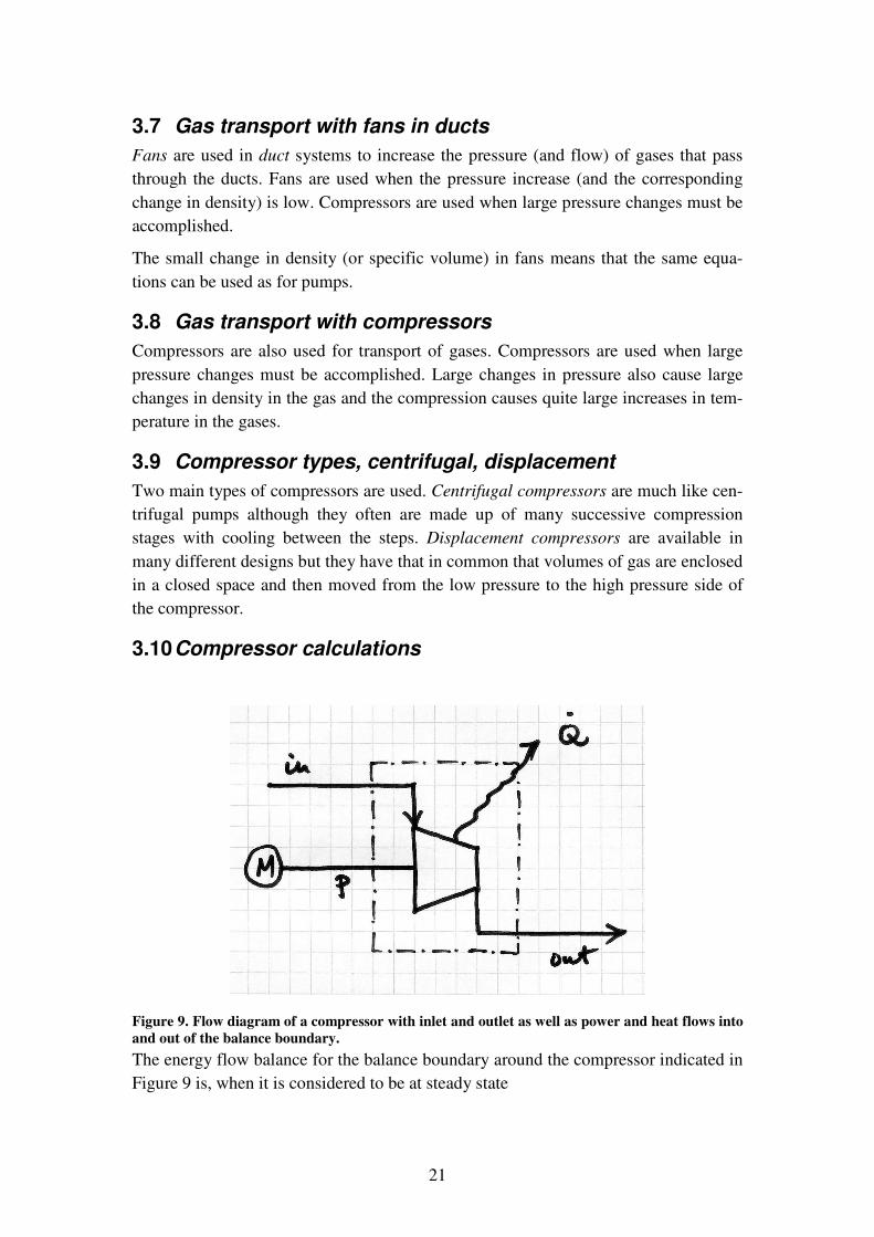
3.10 Compressor calculations
Figure 9. Flow diagram of a compressor with inlet and outlet as well as power and heat flows into and out of the balance boundary. The energy flow balance for the balance boundary around the compressor indicated in Figure 9 is, when it is considered to be at steady state

22
QhmPhm outin NNN +⋅=+⋅
where mO is the mass flow of gas through the compressor, inh and outh are the specific enthalpies of the gas at the inlet and the outlet of the compressor, P is the mechanical power supplied to the compressor and QP is the heat flow from the compressor.
If the balance above is solved for the required mechanical power you get
( ) QhhmP inout NN +−⋅=
The enthalpy is defined by the pressure and temperature of the gas. Commonly the inlet temperature and pressure are known as well as the expected outlet pressure. The outlet temperature depends on the heat flow but also on the efficiency of the compres-sor.
The efficiency is usually defined in relation to an ideal situation where no entropy is generated. The entropy balance for the same balance is
TQsmSsm outprodin
QQQQ+⋅=+⋅
where ins and outs are the specific entropies of the gas at the inlet and the outlet, prodSR is the entropy production in the compressor and T temperature at the boundary
where the heat flow passes through.
If the heat flow is zero (i.e. the compressor is well insulated), then the compression is considered to be adiabatic. This is not always true for real compressors but it is a good approximation.
The ideal situation mentioned earlier that will be used for comparison is that when there is no entropy production in the compressor (isentropic compression) and when the compressor is considered adiabatic. The necessary mechanical power to the com-pressor would then be
( )inout hhmP −′⋅= S
and the entropy balance could be simplified into
outin ss ′=
where outh′ is the specific enthalpy and outs′ is the specific entropy of the gas leaving the compressor in this ideal case.
If the inlet pressure inp and temperature inT are known then the inlet specific enthalpy inh and specific entropy ins are both defined.
The outlet specific entropy outs′ is, according to the equation above, the same as the inlet specific entropy. If the outlet pressure outp is known or set then the temperature

23
outT ′ corresponding to this specific entropy can be calculated and using that also the specific enthalpy outh′ .
The adiabatic conditions can, as was said before, quite well approximate the condi-tions in a compressor, but the isentropic conditions cannot be achieved. The actual conditions are compared to the ideal case using an adiabatic efficiency.
The adiabatic efficiency of a compressor is defined as
inout
inoutad hh
hh−−′
=η
If the heat capacity is considered constant and the gas ideal then it is relatively simple to calculate changes in specific enthalpy and entropy. A change in specific enthalpy between two states 1 and 2 is modeled using
( )1212 TTchh p −⋅≈−
and the corresponding change in specific entropy with
TTUVWWXY⋅−TTUVWWXY⋅≈−1
2
1
212 lnln
pp
MR
TTcss p
where pc is the specific heat capacity of the gas at constant pressure, R is the gas constant (8.314 kJ/kmolK) and M is the molar mass of the gas. Observe that the tem-peratures are given in K.
The temperature of the gas leaving the compressor in the ideal isentropic case can be calculated directly from the entropy balance
0lnln =TTUVWWXY⋅−TTUVWWXY ′⋅=−′
in
out
in
outpinout p
pMR
TT
css
which gives
McR
in
outinout
p
pp
TT⋅ZZ[\]]^_⋅=′
The temperature of the gas leaving the compressor in the real case is calculated using the definition of the adiabatic compressor efficiency
( )( )inoutp
inoutp
inout
inoutad TTc
TTchhhh
−⋅−′⋅
≈−−′
=η
which gives

24
ad
inoutinout
TTTT
η−′
+=
The total power required for the compression then becomes
( )inoutp TTcmP −⋅⋅= `
3.10.1 Example – compressors Natural gas is transported, often long distances, through pipelines from the production fields to the consumers. The natural gas is compressed using compressors to decrease the volume of the gas and the pipe size.
Compressor stations are placed along the pipeline to keep up the necessary pressure. At one of these stations the pressure of the natural gas must be increased from 15 bar to 50 bar. The flow through the pipeline is about 36000 Nm3/h.
Assuming that the gas temperature is 5 °C before the compressor station and that the compressor has an adiabatic efficiency of 70 %, how high will the temperature be af-ter the compressor?
How much cooling must be provided to decrease the temperature to 40 °C?
The higher heating value of natural gas is about 54.4 MJ/kg. If natural gas is used to power the compressor with an efficiency of about 35 % how much gas would be used (percentage of flow in to the compressor station)?
Natural gas is mainly composed of methane (CH4) which has a specific heat capacity of about 2.48 kJ/kgK.
3.11 Typical flow velocities The velocity of the flow in pipes or ducts depends on the pipe or duct size you choose for a certain flow. The velocity in larger pipes is smaller causing a smaller pressure drop in the pipes. Larger pipes also cost more to buy and install so you have to find a pipe size that minimizes the overall cost. It is possible to optimize the selection of pipe size in order to minimize cost but this is generally not done. Most often you just see to it that the flow velocity in the pipe is within a sensible range. The following flow velocities can be used for gas and liquid flows in ducts and pipes.
Gas flow – 10-30 m/s
Liquid flow – 1-2 m/s.

25
4. Heat exchanger systems Whenever you want to move energy in the form of heat from a warmer stream to a colder stream without actually mixing the streams you need a heat exchanger of some kind. (Note that if you need to move heat energy from a colder stream to a warmer stream you need a heat pump instead of a heat exchanger. A refrigerator is a heat pump).
Heat exchangers can be used to set the correct reaction temperature in a reactor, to change the transport properties of fluids, to stop the reactions or to cool the products, for heat recovery after the reactor or to evaporate liquids or condense gases.
There are usually many places where cooling or heating is needed in a process system and it is often possible, or even necessary, to interconnect these heat flows instead of using external heating or cooling. Heat recovery can give economic benefits.
The interconnection of heating and cooling using heat exchangers can be designed and/or analyzed using heat exchanger network models.
4.1 Heat exchanger types The basic idea of a heat exchanger is simple. A thin wall separates the warmer and the colder stream from each other and at the same time leads heat from the warmer to the colder stream. Heat exchangers are commonly used for transport of heat between two gas flows, between gas and liquid flows and between two liquids.
The construction methods and applications of heat exchangers divides them into many different types such as shell and tube heat exchangers, plate heat exchangers, jacketed rectors, steam pipes in furnaces, spiral heat exchangers, condensers and reboilers in distillations columns and so on.
4.2 Heat exchanger modeling, counter current, co-current, real world
Heat exchangers are often modeled using two basic setups – co-current and counter current. Both configurations are shown in Figure 10.
Figure 10. Co-current (left) and counter current (right) heat exchangers.
In a co-current heat exchanger the hot and cold flows go through the heat exchanger in the same direction while they go in opposite directions in a counter current heat ex-changer.
A basic model used to describe the heat flow through the wall of a heat exchanger of any type is

26
lnθ∆⋅⋅= AkQa
where k is the overall heat transfer coefficient and A is the area of the heat transfer surface. The logarithmic mean temperature, lnθ∆ , across the heat transfer surface is defined as
2
1
21ln
lnθθ
θθθ
∆∆
∆−∆=∆
where 1θ∆ is the temperature difference between the warm flow and the cold flow at one end and 2θ∆ is the difference at the other end.
Real world heat exchangers work in a non-ideal way; they might be partially co- and counter current, they might be cross current – but never ideal. One way of compensat-ing is to multiply the log mean temperature with a correction factor F .
lnθ∆⋅⋅⋅= FAkQb
The correction factor depends on the actual type of heat exchanger as well as the tem-peratures of the flows into and out of the heat exchanger.
Figure 11. Correction factors F for two types of heat exchangers (from Perry’s Chemical Engi-neers Handbook). )()( 1221 ttTTR −−= , )()( 1112 tTttS −−=
27
4.3 Overall heat transfer coefficient The heat flow resistance of the heat exchanger wall is more or less constant regardless of temperature and flow. The overall heat flow resistance, on the other hand, is not constant. It changes when deposits are formed on the surface and it changes when the flow velocity and/or the temperature changes.
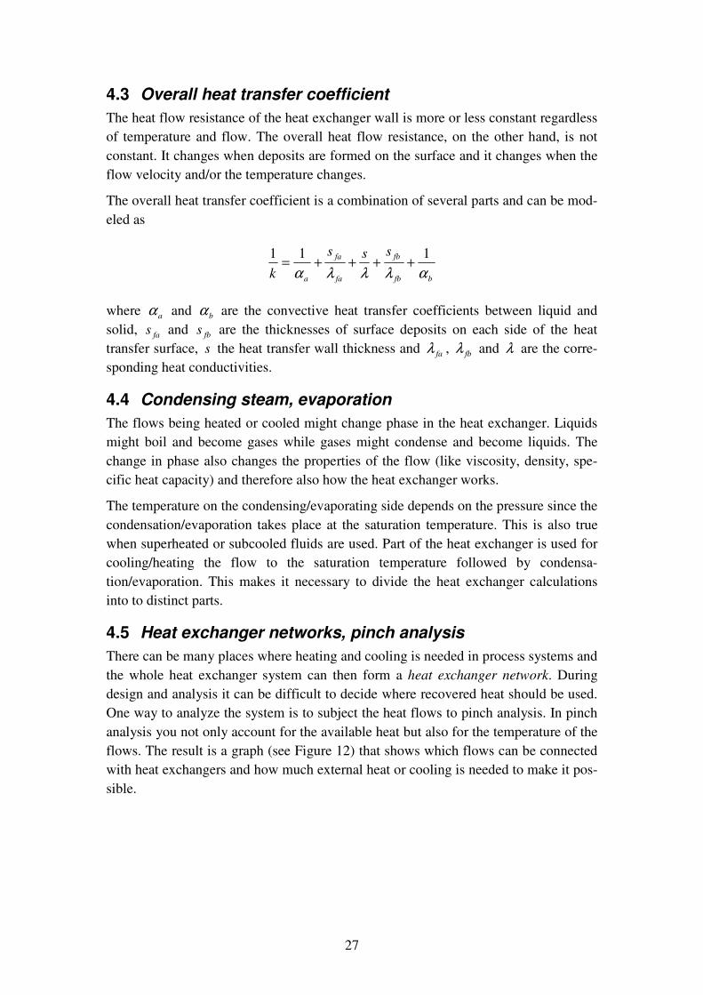
The overall heat transfer coefficient is a combination of several parts and can be mod-eled as
bfb
fb
fa
fa
a
sssk αλλλα
111 ++++=
where aα and bα are the convective heat transfer coefficients between liquid and solid, fas and fbs are the thicknesses of surface deposits on each side of the heat transfer surface, s the heat transfer wall thickness and faλ , fbλ and λ are the corre-sponding heat conductivities.
4.4 Condensing steam, evaporation The flows being heated or cooled might change phase in the heat exchanger. Liquids might boil and become gases while gases might condense and become liquids. The change in phase also changes the properties of the flow (like viscosity, density, spe-cific heat capacity) and therefore also how the heat exchanger works.
The temperature on the condensing/evaporating side depends on the pressure since the condensation/evaporation takes place at the saturation temperature. This is also true when superheated or subcooled fluids are used. Part of the heat exchanger is used for cooling/heating the flow to the saturation temperature followed by condensa-tion/evaporation. This makes it necessary to divide the heat exchanger calculations into to distinct parts.
4.5 Heat exchanger networks, pinch analysis There can be many places where heating and cooling is needed in process systems and the whole heat exchanger system can then form a heat exchanger network. During design and analysis it can be difficult to decide where recovered heat should be used. One way to analyze the system is to subject the heat flows to pinch analysis. In pinch analysis you not only account for the available heat but also for the temperature of the flows. The result is a graph (see Figure 12) that shows which flows can be connected with heat exchangers and how much external heat or cooling is needed to make it pos-sible.

28
0
20
40
60
80
100
120
140
0 1000 2000 3000 4000 5000 6000heat transfer (kW)
tem
pera
ture
(o C)
heatingcooling
Figure 12. Heating and cooling curves used for pinch analysis. The pinch is where the tempera-ture difference is smallest. If the curves cross each other then additional heating or cooling is needed in the system.
4.5.1 Example A compressor produces 4 kg/min compressed air of 10 bar using 25 °C air. The com-pressor is a two stage compressor with an intercooler and an aftercooler that cool the air to 25 °C after each compression step. The air temperature after each compression step is 169 °C.
The compressor also has a separate oil cooler which cools the lubrication oil in the compressor. When the oil flow is 4.2 kg/min and 50 °C when it enters the compressor then it will be 90 °C when it is returned to the cooler. The specific heat capacity of the oil is about 2 kJ/kg°C.
Cold water (4 °C) has been used for cooling in all three coolers. The flow is set so that the water temperature out is no higher than 15 °C.
The heat from the coolers could be used to heat the air that comes into the building at -15 °C to 25 °C. The necessary air flow is about 15 kg/s. Another possible use for the heat is for making hot water. The water comes in at 4 °C and should be heated to 70 °C. The hot water usage is about 8 kg/min.
So there are three hot flows that have to be cooled: air in intercooler, air in aftercooler and lubrication oil in the oil cooler. The heat in these flows could possibly be used to heat the two cold flows: house air, and hot water.
It is of course also possible to use additional heating from the district heating system and additional cooling with cold water using the existing systems.
Calculate the need for additional heating and/or cooling. Draw a graph with heating and cooling curves to see if it is possible to realize this heat recovery using a heat ex-changer network. Data for the hot and cold flows are given in the following table:

29
Id description flow heat capacity inlet outlet
H1 air in intercooler 4 kg/min 1.0 kJ/kgK 169 °C 25 °C
H2 air in aftercooler 4 kg/min 1.0 kJ/kgK 169 °C 25 °C
H3 oil in oil cooler 4.2 kg/min 2.0 kJ/kgK 90 °C 50 °C
H district heating x kg/min 4.2 kJ/kgK 120 °C 50 °C
C1 house air 15 kg/min 1.0 kJ/kgK -15 °C 25 °C
C2 hot tap water 8 kg/min 4.2 kJ/kgK 4 °C 70 °C
C cold tap water x kg/min 4.2 kJ/kgK 4 °C 15 °C
30
5. Economic analysis – modeling and selection One important part of process design is to make choices. Many of these choices are made based on economic evaluation of the design or designs that we generate.
When the design has reached the stage, where the major pieces of equipment have been sized (heat transfer surface, pump capacity, mixer power, reactor size etc.) then can a preliminary estimate of the cost for the plant be made.
Sinnott (Coulson&Richardson’s Chemical Engineering Volume 6 – Chemical Engi-neering and Design, chapter 6) shows some examples on how estimates of this type can be made.


