Basics of Digital Communications

1

Basics of Digital Communications

1.1 Orthogonal Signals and Vectors

The concept of orthogonal signals is essential for the understanding of OFDM (orthogonalfrequency division multiplexing) and CDMA (code division multiple access) systems. Inthe normal sense, it may look like a miracle that one can separately demodulate overlappingcarriers (for OFDM) or detect a signal among other signals that share the same frequencyband (for CDMA). The concept of orthogonality unveils this miracle. To understand theseconcepts, it is very helpful to interpret signals as vectors. Like vectors, signals can beadded, multiplied by a scalar, and they can be expanded into a base. In fact, signals fit intothe mathematical structure of a vector space. This concept may look a little bit abstract.However, vectors can be visualized by geometrical objects, and many conclusions canbe drawn by simple geometrical arguments without lengthy formal derivations. So it isworthwhile to become familiar with this point of view.

1.1.1 The Fourier base signals

To visualize signals as vectors, we start with the familiar example of a Fourier series. Forreasons that will become obvious later, we do not deal with a periodic signal, but cutoff outside the time interval of one period of length T . This means that we consider awell-behaved (e.g. integrable) real signal x(t) inside the time interval 0 ≤ t ≤ T and setx(t) = 0 outside. Inside the interval, the signal can be written as a Fourier series

x(t) = a0

2+

∞∑k=1

ak cos

(2π

k

Tt

)−

∞∑k=1

bk sin

(2π

k

Tt

). (1.1)

The Fourier coefficients ak and bk are given by

ak = 2

T

∫ T

0cos

(2π

k

Tt

)x(t) dt (1.2)

Theory and Applications of OFDM and CDMA Henrik Schulze and Christian Luders 2005 John Wiley & Sons, Ltd

2 BASICS OF DIGITAL COMMUNICATIONS

and

bk = − 2

T

∫ T

0sin

(2π

k

Tt

)x(t) dt. (1.3)

These coefficients are the amplitudes of the cosine and (negative) sine waves at the respec-tive frequencies fk = k/T . The cosine and (negative) sine waves are interpreted as a basefor the (well-behaved) signals inside the time interval of length T . Every such signal canbe expanded into that base according to Equation (1.1) inside that interval. The underlyingmathematical structure of the Fourier series is similar to the expansion of an N -dimensionalvector x ∈ RN into a base {vi}Ni=1 according to

x =N∑

i=1

αivi . (1.4)

The base {vi}Ni=1 is called orthonormal if two different vectors are orthogonal (perpendi-cular) to each other and if they are normalized to length one, that is,

vi · vk = δik,

where δik is the Kronecker Delta (δik = 1 for i = k and δik = 0 otherwise) and the dotdenotes the usual scalar product

x · y =N∑

i=1

xiyi = xT y

for real N -dimensional vectors. In that case, the coefficients αi are given by

αi = vi · x.

For an orthonormal base, the coefficients αi can thus be interpreted as the projections ofthe vector x onto the base vectors, as depicted in Figure 1.1 for N = 2. Thus, αi can beinterpreted as the amplitude of x in the direction of vi .

�

�

��

v1

v2

α1

α2

x

Figure 1.1 A signal vector in two dimensions.

BASICS OF DIGITAL COMMUNICATIONS 3

The Fourier expansion (1.1) is of the same type as the expansion (1.4), except that thesum is infinite. For a better comparison, we may write

x(t) =∞∑i=0

αivi(t)

with the normalized base signal vectors vi(t) defined by

v0(t) =√

1

T�

(t

T− 1

2

)

and

v2k(t) =√

2

Tcos

(2π

k

Tt

)�

(t

T− 1

2

)for even i > 0 and

v2k+1(t) = −√

2

Tsin

(2π

k

Tt

)�

(t

T− 1

2

)

for odd i with coefficients given by

αi =∫ ∞

−∞vi(t)x(t) dt,

that is,α2k =

√T /2ak

andα2k+1 =

√T /2bk.

Here we have introduced the notation �(x) for the rectangular function, which takes thevalue one between x = −1/2 and x = 1/2 and zero outside. Thus, �(x − 1/2) is therectangle between x = 0 and x = 1. The base of signals vi(t) fulfills the orthonormalitycondition ∫ ∞

−∞vi(t)vk(t) dt = δik. (1.5)

We will see in the following text that this just means that the Fourier base forms a set oforthogonal signals. With this interpretation, Equation (1.5) says that the base signals fordifferent frequencies are orthogonal and, for the same frequency fk = k/T , the sine andcosine waves are orthogonal.

We note that the orthonormality condition and the formula for αi are very similar tothe case of finite-dimensional vectors. One just has to replace sums by integrals. A similargeometrical interpretation is also possible; one has to regard signals as vectors, that is,identify vi(t) with vi and x(t) with x. The interpretation of αi as a projection on vi isobvious. For only two dimensions, we have x(t) = α1v1(t) + α2v2(t) , and the signals canbe adequately described by Figure 1.1. In this special case, where v1(t) is a cosine signaland v2(t) is a (negative) sine signal, the figure depicts nothing else but the familiar phasordiagram. However, this is just a special case of a very general concept that applies to manyother scenarios in communications.


Before we further discuss this concept for signals by introducing a scalar product forsignals, we continue with the complex Fourier transform. This is because complex signalsare a common tool in communications engineering.

Consider a well-behaved complex signal s(t) inside the time interval [0, T ] that vanishesoutside that interval. The complex Fourier series for that signal can be written as

s(t) =∞∑

k=−∞αkvk(t) (1.6)

with the (normalized) complex Fourier base functions

vk(t) =√

1

Texp

(j2π

k

Tt

)�

(t

T− 1

2

). (1.7)

The base functions are orthonormal in the sense that∫ ∞

−∞v∗

i (t)vk(t) dt = δik. (1.8)

holds. The Fourier coefficient αk will be obtained from the signal by the Fourier analyzer.This is a detection device that performs the operation

αk =∫ ∞

−∞v∗

i (t)s(t) dt. (1.9)

This coefficient is the complex amplitude (i.e. amplitude and phase) of the wave at frequencyfk . It can be interpreted as the component of the signal vector s(t) in the direction of thebase signal vector vk(t), that is, we interpret frequency components as vector componentsor vector coordinates.

Example 1 (OFDM Transmission) Given a finite set of complex numbers sk that carrydigitally encoded information to be transmitted, we may use the complex Fourier series forthis purpose and transmit the signal

s(t) =K∑

k=0

skvk(t). (1.10)

The transmitter performs a Fourier synthesis. In an ideal transmission channel with perfectsynchronization and no disturbances, the transmit symbols sk can be completely recovered atthe receiver by the Fourier analyzer that plays the role of the detector. One may send K newcomplex symbols during every time slot of length T by performing the Fourier synthesis forthat time slot. At the receiver, the Fourier analysis is done for every time slot. This methodis called orthogonal frequency division multiplexing (OFDM). This name is due to the factthat the transmit signals form an orthogonal base belonging to different frequencies fk .We will see in the following text that other – even more familiar – transmission setups useorthogonal bases.


1.1.2 The signal space

A few mathematical concepts are needed to extend the concept of orthogonal signals toother applications and to represent the underlying structure more clearly. We consider (realor complex) signals of finite energy, that is, signals s(t) with the property∫ ∞

−∞|s(t)|2 dt < ∞. (1.11)

The assumption that our signals should have finite energy is physically reasonable and leadsto desired mathematical properties. We note that this set of signals has the property of avector space, because finite-energy signals can be added or multiplied by a scalar, resultingin a finite-energy signal. For this vector space, a scalar product is given by the following:

Definition 1.1.1 (Scalar product of signals) In the vector space of signals with finite en-ergy, the scalar product of two signals s(t) and r(t) is defined as

〈s, r〉 =∫ ∞

−∞s∗(t)r(t) dt. (1.12)

Two signals are called orthogonal if their scalar product equals zero. The Euclidean normof the signal is defined by ‖s‖ = √〈s, s〉, and ‖s‖2 = 〈s, s〉 is the signal energy. ‖s − r‖2 iscalled the squared Euclidean distance between s(t) and r(t).

We add the following remarks:

• This scalar product has a structure similar to the scalar product of vectors s =(s1, . . . , sK)T and r = (r1, . . . , rK)T in a K-dimensional complex vector space givenby

s†r =K∑

k=1

s∗k rk,

where the dagger (†) means conjugate transpose. Comparing this expression with thedefinition of the scalar product for continuous signals, we see that the sum has to bereplaced by the integral.

• It is a common use of notation in communications engineering to write a function withan argument for the function, that is, to write s(t) for a signal (which is a functionof the time) instead of s, which would be the mathematically correct notation. Inmost cases, we will use the engineer’s notation, but we write, for example, 〈s, r〉 andnot 〈s(t), r(t)〉, because this quantity does not depend on t . However, sometimes wewrite s instead of s(t) when it makes the notation simpler.

• In mathematics, the vector space of square integrable functions (i.e. finite-energysignals) with the scalar product as defined above is called the Hilbert space L2(R).It is interesting to note that the Hilbert space of finite-energy signals is the same asthe Hilbert space of wave functions in quantum mechanics. For the reader who isinterested in details, we refer to standard text books in mathematical physics (see e.g.(Reed and Simon 1980)).


Without proof, we refer to some mathematical facts about that space of signals with finiteenergy (see e.g. (Reed and Simon 1980)).

• Each signal s(t) of finite energy can be expanded into an orthonormal base, that is,it can be written as

s(t) =∞∑

k=1

αkvk(t) (1.13)

with properly chosen orthonormal base signals vk(t). The coefficients can be obtainedfrom the signal as

αk = 〈vk, s〉 . (1.14)

The coefficient αk can be interpreted as the component of the signal vector s in thedirection of the base vector vk .

• For any two finite energy signals s(t) and r(t), the Schwarz inequality

|〈s, r〉| ≤ ‖s‖ ‖r‖holds. Equality holds if and only if s(t) is proportional to r(t).

• The Fourier transform is well defined for finite-energy signals. Now, let s(t) and r(t)

be two signals of finite energy, and S(f ) and R(f ) denote their Fourier transforms.Then,

〈s, r〉 = 〈S, R〉holds. This fact is called Plancherel theorem or Rayleigh theorem in the mathematicalliterature (Bracewell 2000). The above equality is often called Parseval’s equation .As an important special case, we note that the signal energy can be expressed eitherin the time or in the frequency domain as

E =∫ ∞

−∞|s(t)|2 dt =

∫ ∞

−∞|S(f )|2 df.

Thus, |S(f )|2 df is the energy in an infinitesimal frequency interval of width df ,and |S(f )|2 can be interpreted as the spectral density of the signal energy.

In communications, we often deal with subspaces of the vector space of finite-energysignals. The signals of finite duration form such a subspace. An appropriate base of thatsubspace is the Fourier base. The Fourier series is then just a special case of Equation(1.13) and the Fourier coefficients are given by Equation (1.14). Another subspace is thespace of strictly band-limited signals of finite energy. From the sampling theorem we knowthat each such signal s(t) that is concentrated inside the frequency interval between −B/2and B/2 can be written as a series

s(t) =∞∑

k=−∞s(k/B)sinc (Bt − k) (1.15)

with sinc (x) = sin (πx)/(πx).We define a base as follows:


Definition 1.1.2 (Normalized sinc base) The orthonormal sinc base for the bandwidth B/2is given by the signals

ψk(t) =√

B sinc (Bt − k) . (1.16)

We note that√

B ψ0(t) is the impulse response of an ideal low-pass filter of bandwidthB/2, so that the sinc base consists of delayed and normalized versions of that impulseresponse. From the sampling theorem, we conclude that these ψk(t) are a base of thesubspace of strictly band-limited functions. By looking at them in the frequency domain,we easily see that they are orthonormal. From standard Fourier transform relations, we seethat the Fourier transform �k(f ) of ψk(t) is given by

�k(f ) = 1√B

� (f/B) e−j2πkf/B.

Thus, �k(f ) is just a Fourier base function for signals concentrated inside the frequencyinterval between −B/2 and B/2. This base is known to be orthogonal. Thus, we rewritethe statement of the sampling theorem as the expansion

s(t) =∞∑

k=−∞skψk(t)

into the orthonormal base ψk(t). From the sampling theorem, we know that

sk = 1√B

s(k/B)

holds. The Fourier transform of this signal is given by

S(f ) =∞∑

k=−∞sk�k(f ).

This is just a Fourier series for the spectral function that is concentrated inside the frequencyinterval between −B/2 and B/2. The coefficients are given by

sk = 〈ψk, s〉 = 〈�k, S〉 .

This relates the coefficients of a Fourier expansion of a signal S(f ) in the frequency domainto the samples of the corresponding signal s(t) in the time domain. As we have seen fromthis discussion, the Fourier base and the sinc base are related to each other by interchangingthe role of time and frequency.

1.1.3 Transmitters and detectors

Any linear digital transmission setup can be characterized as follows: As in the OFDMExample 1, for each transmission system we have to deal with a synthesis of a signal (atthe transmitter site) and the analysis of a signal (at the receiver site). Given a finite set{sk}Kk=1 of coefficients that carry the information to be transmitted, we choose a base gk(t)

to transmit the information by the signal

s(t) =K∑

k=1

skgk(t). (1.17)


Definition 1.1.3 (Transmit base, pulses and symbols) In the above sum, each signal gk(t)

is called a transmit pulse, the set of signals {gk(t)}Kk=1 is called the transmit base, and sk

is called a transmit symbol. The vector s = (s1, . . . , sK)T is called the transmit symbolvector.

Note that in the terminology of vectors, the transmit symbols sk are the coordinates of thesignal vector s(t) corresponding to the base gk(t).

If the transmit base is orthonormal, then, for an ideal transmission channel, the infor-mation symbols sk can be recovered completely as the projections onto the base. Thesescalar products

sk = 〈gk, s〉 =∫ ∞

−∞g∗

k (t)s(t) dt (1.18)

can also be written as

sk =[∫ ∞

−∞g∗

k (τ − t)s(τ ) dτ

]t=0

= [g∗

k (−t) ∗ s(t)]t=0 . (1.19)

This means that the detection of the information sk transmitted by gk(t) is the output of thefilter with impulse response g∗

k (−t) sampled at t = 0. This filter is usually called matchedfilter, because it is matched to the transmit pulse g(t).

Definition 1.1.4 (Detector and matched filter) Given a transmit pulse g(t), the corres-ponding matched filter is the filter with the impulse response g∗(−t). The detector Dg forg(t) is defined by the matched filter output sampled at t = 0, that is, by the detector outputDg[r] given by

Dg[r] =∫ ∞

−∞g∗(t)r(t) dt (1.20)

for any receive signal r(t). If two transmit pulses g1(t) and g2(t) are orthogonal, then thecorresponding detectors are called orthogonal.

Thus, a detector extracts a (real or complex) number. This number carries the informa-tion. The detector may be visualized as depicted in Figure 1.2.

The matched filter has an interesting property: if a transmit pulse is corrupted by white(not necessarily Gaussian) noise, then the matched filter is the one that maximizes thesignal-to-noise ratio (SNR) for t = 0 at the receiver end (see Problem 6).

We add the following remarks:

• For a finite-energy receive signal r(t), Dg[r] = 〈g, r〉 holds. However, we usuallyhave additive noise components in the signal at the receiver, which are typically notof finite energy, so that the scalar product is not defined.

� �r(t) Dg Dg[r]

Figure 1.2 Detector.


�

� �

�r(t)

g(t)

Dg

Dr

Dg[r]

Dr[g]

Figure 1.3 Input and detector pulses.

• The detector Dg[r] compares two signals: in principle, it answers the question ‘Howmuch of r(t) looks like g(t)?’. The role of receive signal and the pulse can beinterchanged according to

Dg[r] = D∗r [g],

as Figure 1.3 depicts.

• The Fourier analyzer given by Equation (1.9) is a set of orthogonal detectors. Thesinc base is another set of orthogonal detectors.

• For an orthonormal base, the energy of the transmit signal equals the energy of thevector of transmit symbols, that is,

E =∫ ∞

−∞|s(t)|2 dt =

K∑k=1

|sk|2,

or more compactly written as E = ‖s‖2 = ‖s‖2 . For the proof, we refer to Problem 1.

The following example shows that the familiar Nyquist pulse shaping can be understoodas an orthogonality condition.

Example 2 (The Nyquist Base) Consider a transmission pulse g(t) with the property∫ ∞

−∞g∗(t)g(t − kTS) dt = δ[k] (1.21)

for a certain time interval TS , that is, the pulse g(t) and its versions time-shifted by kTS buildan orthonormal base. This property also means that the pulse shape h(t) = g∗(−t) ∗ g(t) isa so-called Nyquist pulse that satisfies the first Nyquist criterion h(kTS) = δ[k] and allows atransmission that is free of intersymbol interference (ISI). For the Fourier transforms G(f )

and H(f ) of g(t) and h(t), the relation H(f ) = |G(f )|2 holds. Therefore, g(t) is oftencalled a sqrt-Nyquist pulse. If we define gk(t) = g(t − kTS) as the pulse transmitted at timekTS , the condition (1.21) is equivalent to

〈gi, gk〉 = δik. (1.22)


We then call the base formed by the signals gk(t) a (sqrt-) Nyquist base. Equation (1.22)means that if the pulse is transmitted at time kTS , the detector for the pulse transmitted attime iTS has output zero unless i = k. Thus, the pulses do not interfere with each other.

We note that in practice the pulse g(t) is the impulse response of the transmit filter, thatis, the pulse-shaping filter that will be excited by the transmit symbols sk . The correspondingmatched filter g∗(−t) is the receive filter. Its output will be sampled once in every symbolclock TS to recover the symbols sk . The impulse response of the whole transmission chainh(t) = g∗(−t) ∗ g(t) must be a Nyquist pulse to ensure symbol recovery without intersymbolinterference.

The Nyquist criterionh(kTS) = δ[k]

in the time domain can be equivalently written in the frequency domain as

∞∑k=−∞

H

(f − k

TS

)= TS,

where H(f ) is the Fourier transform of h(t). Familiar Nyquist pulses like raised cosine(RC) pulses are usually derived from this criterion in the frequency domain (see e.g. (Proakis2001)). In the following text, we shall show a simple method to construct Nyquist pulsesin the time domain.

Obviously, every pulse of the shape

h(t) = u(t) · sinc (t/TS)

satisfies the Nyquist criterion in the time domain. u(t) should be a function that improvesthe decay of the pulse. In the frequency domain, this is equivalent to

H(f ) = TS U(f ) ∗ � (f TS) ,

where U(f ) is the Fourier transform of u(t). The convolution with U(f ) smoothens thesharp flank of the rectangle. Writing out the convolution integral leads to

H(f ) = TS

(V

(f + 1

2TS

)− V

(f − 1

2TS

))

with

V (f ) =∫ f

−∞U(x) dx.

V (f ) is a function that describes the flank of the filter given by H(f ).

One possible choice for U(f ) is

U(f ) = π

2αTS cos

(π

αf TS

)�

(1

αf TS

), 0 ≤ α ≤ 1

with a constant α between that we call the rolloff factor . The corresponding time domainfunction obviously given by

u(t) = π

4

(sinc

(α

t

TS

+ 1

2

)+ sinc

(α

t

TS

− 1

2

)),


which equals the expression

u(t) = cos (παt/TS)

1 − (2αt/TS)2 .

The filter flank is obtained by integration as

V (f ) =

0 : f TS ≤ −α/21

2

(1 + sin

(π

αf TS

)): −α/2 ≤ f TS ≤ α/2

1 : f TS ≥ α/2.

(1.23)

The shape of the filter is then given by the familiar expression

H(f ) =

TS : 2|f |TS ≤ 1 − α

TS

2

(1 − sin

(π

α

(|f |TS − 1

2

))): 1 − α ≤ 2|f |TS ≤ 1 + α

0 : 2|f |TS ≥ 1 + α.

(1.24)

The corresponding pulse is

h(t) = sinc (t/TS) · cos (παt/TS)

1 − (2αt/TS)2 . (1.25)

Other Nyquist pulses than these so-called raised cosine (RC) pulses are possible. AGaussian

u(t) = exp(− (βt/TS)

2)guarantees an exponential decay in both the time and the frequency domain. β is a shapingparameter similar to the rolloff factor α. The Fourier transform U(f ) of u(t) is given by

U(f ) =√

πT 2S /β2 exp

(− (πTSf/β)2) ,

and the filter flank is

V (f ) = 1

2

(1 + erf

(π

βTSf

)).

The filter curve is then given by

H(f ) = 1

2TS

(erf

(π

β

(TSf + 1

2

))− erf

(π

β

(TSf − 1

2

))). (1.26)

The RC pulse and the Gaussian Nyquist pulse

h(t) = sinc (t/TS) · exp(− (βt/TS)

2) (1.27)

have a very similar shape if we relate α and β in such a way that their flanks V (f ) havethe same first derivative at f = 0. This is the case for

β = 2α

π.


–1 –0.8 –0.6 –0.4 –0.2 0 0.2 0.4 0.6 0.8 10

0.1

0.2

0.3

0.4

0.5

0.6

0.7

0.8

0.9

1

fTS

H(f

)

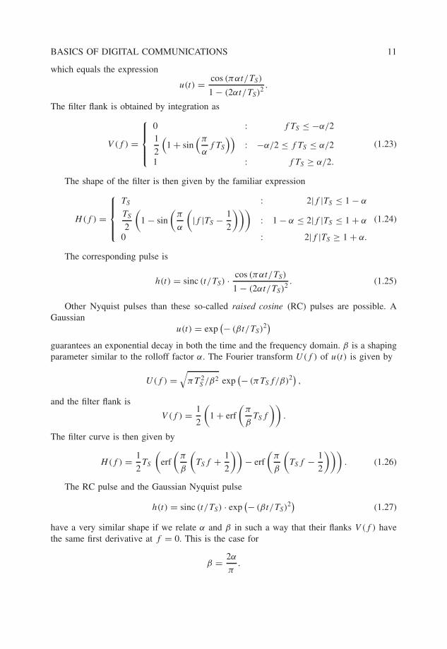
Figure 1.4 RC and Gaussian Nyquist filter shape for α = 0.2.

–1 –0.8 –0.6 –0.4 –0.2 0 0.2 0.4 0.6 0.8 1–20

–18

–16

–14

–12

–10

–8

–6

–4

–2

0

fTS

10 lo

g H

(f)

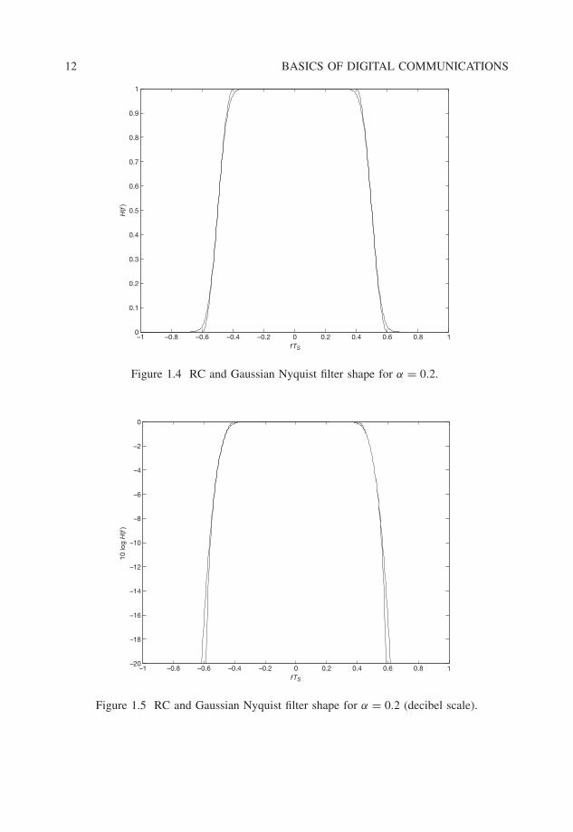
Figure 1.5 RC and Gaussian Nyquist filter shape for α = 0.2 (decibel scale).


–5 –4 –3 –2 –1 0 1 2 3 4 5–0.4

–0.2

0

0.2

0.4

0.6

0.8

1

t/TS

h(t)

Figure 1.6 RC and Gaussian Nyquist pulse shape for α = 0.2.

For this case and α = 0.2, both filter shapes are depicted in Figure 1.4, and with alogarithmic scale, in Figure 1.5. The Gaussian shaping is slightly broader at the outerflanks, but the difference is very small even on the logarithmic scale. Figure 1.6 shows thecorresponding pulses. The Gaussian pulse has slightly smaller amplitudes, but the differenceis very small. Of course, both curves differ significantly in their asymptotic behavior (whichcan be seen on a logarithmic scale), but this is in a region where pulses are practicallyzero.

1.1.4 Walsh functions and orthonormal transmit bases

In this subsection, we introduce the Walsh functions that play an important role in CDMAsignaling. We regard them as an example to discuss an orthonormal base that can beinterpreted as a base of signals or as a base in an Euclidean space.

The M × M Walsh–Hadamard (WH) matrices HM , where M is a power of two, aredefined by H1 = 1 and the recursive relation

HM =[

HM/2 HM/2

HM/2 −HM/2

].

For example, the matrix H4 is given by

H4 =

1 1 1 11 −1 1 −11 1 −1 −11 −1 −1 1

.


The column vectors of the WH matrix are pairwise orthogonal but not normalized to one.We may divide them by their length

√M to obtain the normalized WH vectors gk related

to HM by √M HM = G = [

g1, . . . , gM

]. (1.28)

The column vectors are orthonormal, that is,

gi · gk = δik.

For a given value of M , the Walsh functions gk(t), k = 1, . . . , M are functions defined ona time interval t ∈ [0, TS] that are piecewise constant on time sub-intervals (called chips) ofduration Tc = TS/M . The sign of the function on the ith time sub-interval (i = 1, . . . , M)is given by the ith component hik of the kth column vector in the WH matrix HM . Theabsolute value is normalized to 1/

√TS to obtain an orthonormal signal base, that is,

〈gi, gk〉 = δik.

Outside the interval t ∈ [0, TS], the Walsh functions vanish. For M = 8, the Walsh functionsare depicted in Figure 1.7.

We can write the normalized Walsh functions as

gk(t) =M∑i=1

gikci(t), (1.29)

where gik = hik/√

M , and the chip pulse ci(t) is defined by ci(t) = 1/√

Tc in the ith chipinterval and zero outside. Obviously

〈ci, ck〉 = δik

holds, that is, the chip pulses are orthonormal. Given the transmit base {gk(t)}Mk=1, we maytransmit information carried by the symbols {sk}Mk=1 by using the signal

s(t) =M∑

k=1

skgk(t). (1.30)

Instead of {gk(t)}Mk=1, we can use the equivalent discrete base {gk}Mk=1 and transmit thevector

s =M∑

k=1

skgk. (1.31)

This representation allows the geometrical interpretation of the transmit signal as a vectors in an M-dimensional Euclidean space. The transmit symbols sk are the components ofthe vector s in the orthonormal Walsh–Hadamard base {gk}Mk=1, which is a rotated versionof the canonical Euclidean base e1 = (1, 0, 0, . . . , 0)T , e2 = (0, 1, 0, . . . , 0)T , . . . , eM =(0, . . . , 0, 1)T with the rotation given by the matrix G. Equation (1.29) is the coordinatetransform corresponding to the base transform from the base of chip pulses to the base ofnormalized Walsh functions. Thus, the chip pulse base can be identified with the canonicalEuclidean base. For an ideal channel, the components sk of the vector s can be completely


�

�

�

�

�

�

��

� �

�

TS

t

t

t

t

t

t

t

t

Tc

g1(t)

g2(t)

g3(t)

g4(t)

g5(t)

g6(t)

g7(t)

g8(t)

Figure 1.7 Walsh functions for M = 8.

recovered by projecting the receive vector on the base vectors gk. For M = 2, the situationis depicted in Figure 1.8.

The orthogonality of the base can be interpreted as the existence of M independentchannels without cross talk as illustrated in Figure 1.9 for M = 2. The orthogonal detectorsDgi

correspond to the projections on the base vectors. If the symbols {sk}Mk=1 are part of thesame data stream, M symbols are transmitted in parallel via M channels during the timeinterval TS . Orthogonality means absence of ISI between these channels. Another possibilityis to use the M channels to transmit M independent data streams, each of them with therate of one symbol transmitted during the time interval TS . In that case, the orthogonalityis used for multiplexing or multiple access, as it is the situation in CDMA (code divisionmultiple access). Each Walsh function corresponds to another code that may be allocated to


s

g1

s1

s2

g2

Figure 1.8 The orthonormal Walsh–Hadamard base.

�

�

�

�

�

�

DEMUX

MUXs1, s2 s1, s2

Dg1s1g1

s2g2

s1

s2Dg2

TX/

Figure 1.9 Orthogonal channels.

a certain user in a mobile radio scenario. The downlink of the Qualcomm CDMA systemIS-95 (now called cdmaOne, see Subsection 5.5.6) is an example for such a setup (see thediscussion in Chapter 5).

Walsh functions may also be used for orthogonal signaling. In that case the term Walshmodulation is often used. This transmission scheme is very robust against noise, but it leadsto a significant spreading of the bandwidth. For CDMA systems, both properties togetherare desirable. This modulation scheme is used in the uplink of the Qualcomm system IS-95.In a setup with orthogonal Walsh modulation, only one base pulse gk(t) will be transmittedduring the time period TS . One can transmit log2(M) bits during TS by selecting one ofthe M base pulses. The transmit signal during this time period is simply given by

s(t) =√

ES gk(t)


ors =

√ES gk,

where√

ES is the energy of the signal in the time period of length TS .We note that all the properties discussed in this subsection hold not only for the

piecewise constant chip pulse but also for any set of chip pulses ci(t) that satisfies theorthonormality condition 〈ci, ck〉 = δik , and the base signal given by Equation (1.30) holds.One may, for example, choose any Nyquist base for the pulses ci(t) with smoother pulseshape than the rectangular pulses in order to get better spectral properties. It is also possibleto use the Fourier base pulse for ci(t) in Equation (1.30), resulting in multicarrier (MC-)CDMA. Then, a chip may be interpreted as a frequency pulse rather than a time pulse.

1.1.5 Nonorthogonal bases

Orthonormal transmit bases have desirable properties for simple detection. However, some-times it is necessary to deal with nonorthogonal bases. This may be the case when atransmission channel corrupts the orthogonality. For example, the channel may introduceISI, so the ISI-free Nyquist base used for transmission will be convolved by the channelimpulse response resulting in nonorthogonal base vectors. In such a case, the channel mustbe regarded as a part of the transmit setup.

Now, let the pulses bk(t) be such a base of nonorthogonal, but linearly independent,transmit pulses and let xk, k = 1, . . . , K be the finite set of transmit symbols. The trans-mitted signal is then given by

s(t) =K∑

k=1

xkbk(t). (1.32)

There exists an orthonormal base {ψk}Kk=1 for the finite-dimensional vector space spannedby the transmit pulses bk(t), which can be obtained using the Gram–Schmidt algorithm.The two bases are related by the base transform

bk(t) =K∑

i=1

bikψi(t) (1.33)

with bik = 〈ψi, bk〉. We take the scalar product of Equation (1.32) with the vector ψi(t)

and obtain

si =K∑

k=1

xkbik,

where we have defined si = 〈ψi, s〉. This is a coordinate transform of the coordinates xk ofthe signal corresponding to the nonorthogonal base bk(t) to the coordinates sk correspondingto the orthonormal base ψk(t) by writing

s(t) =K∑

k=1

skψk(t).

Defining x = (x1, . . . , xk)T and s = (s1, . . . , sk)

T , the coordinate transform can be writtenin the more compact matrix notation as

s = Bx


with the matrix B of entries bik . Because this coordinate transform is invertible, the transmitsymbols xk can be recovered from the sk by x = B−1s. Thus, in a channel without noise, thereceiver may use the detector outputs corresponding to the orthonormal base and transformthem by using the inverse matrix. However, in a noisy channel, this inversion is not optimalfor the detection, because it causes noise enhancement.

For a receive signal r(t), the detector outputs in the nonorthogonal base

yk = Dbk[r] =

∫ ∞

−∞b∗

k (t)r(t) dt

are related to the detector outputs

rk = Dψk[r] =

∫ ∞

−∞ψ∗

k (t)r(t) dt

in the orthogonal base by

yk =K∑

i=1

b∗ikri

or, in matrix notation, byy = B†r.

Because this transform is invertible, the detector outputs rk can be recovered from the yk

by r = (B†)−1

y.

1.2 Baseband and Passband Transmission

It is convenient to describe a digitally modulated passband signal by a so-called complexequivalent low-pass or complex baseband signal. Let s(t) be a strictly band-limited1 pass-band signal of bandwidth B centered around a carrier frequency f0. We have chosen thesign ˜ for the signal s(t) to indicate a wave for the RF signal. It is possible to completelydescribe s(t) by its equivalent low-pass signal s(t) of bandwidth B/2. Both signals arerelated by

s(t) =√

2 {s(t)ej2πf0t }. (1.34)

This one-to-one correspondence between both signals s(t) and s(t) is easy to visualizeif we look at them in the frequency domain. Writing S(f ) and S(f ) for their respectiveFourier transforms, Equation (1.34) is equivalent to

S(f ) = 1√2

(S (f − f0) + S∗ (−f − f0)

).

This is because, in Equation (1.34), multiplication with the exponential corresponds to afrequency shift by f0, and taking the real part corresponds (up to a factor of 2) to adding

1We note that strictly band-limited signals do not exist in reality. This is due to the fact that a strictly band-limited signal cannot be time limited, which should be the case for signals in reality. However, it is mathematicallyconvenient to make this assumption, always keeping in mind that this is only an approximation and the accuracyof this model has to be discussed for any practical case.


�

�

�

�

��

��

��

��

��

� �

� � � �f0

0 f

|S(f )|2

f0

(a)

(b)

|S(f )|2

−f0

B

B B

Figure 1.10 Equivalence of (a) passband and (b) complex baseband representation of thesame signal.

the negative spectral component (see Problem 2). Figure 1.10 shows the energy spectraldensities |S(f )|2 and |S(f )|2 for both signals. We have chosen a normalization such thatthe total energy of both signals is the same, that is,∫ ∞

−∞|s(t)|2 dt =

∫ ∞

−∞|s(t)|2 dt

and ∫ ∞

−∞|S(f )|2 df =

∫ ∞

−∞|S(f )|2 df.

It is obvious from the figure that both signals S(f ) and S(f ) are only located at differentfrequencies, but they carry the same information. The signal S(f ) can be obtained fromS(f ) by a frequency shift by −f0 followed by an ideal low-pass filter of bandwidth B/2,and a scaling by the factor

√2. Denoting the low-pass filter impulse response by (t), this

operation can be written in the time domain as

s(t) = (t) ∗[√

2 exp (−j2πf0t) s(t)]. (1.35)

We note that the upconversion from s(t) to s(t) as described by Equation (1.34) doublesthe bandwidth of the two components (real and imaginary part) of the baseband signal,


resulting in one signal of bandwidth B instead of two (real) signals of bandwidth B/2. Wewrite s(t) = x(t) + jy(t) and call the real part, x(t), the I- (inphase) and the imaginarypart y(t) the Q- (quadrature) component. Both components together are called quadraturecomponents. Equation (1.34) can then be written as

s(t) =√

2 x(t) cos (2πf0t) −√

2 y(t) sin (2πf0t) , (1.36)

which is the superposition of the cosine-modulated I-component and the (negative) sine-modulated Q-component. It is an important fact that the passband of width B is shared bytwo separable channels: one is the cosine and the other is the sine channel. We shall seethat the I-component modulated by the cosine is orthogonal to the Q-component modulatedby the sine. Thus, they behave like two different channels (without cross talk) that can beindividually used for transmission. We will further see that both the I-modulation and theQ-modulation leave scalar products invariant. To make the following treatment simpler, wefirst introduce a formal shorthand notation for the quadrature modulator and demodulator.

1.2.1 Quadrature modulator

First we define the quadrature modulator as given by Equation (1.36), but separately forboth components.

Definition 1.2.1 (I- and Q-modulator) Let x(t) and y(t) be some arbitrary real signals.Let (t) denote the impulse response of an ideal low-pass filter of bandwidth B/2. Letf0 > B/2. We then define the modulated signals x(t) and y(t) as

x(t) =√

2 cos (2πf0t) [(t) ∗ x(t)] (1.37)

andy(t) = −

√2 sin (2πf0t)

[(t) ∗ y(t)

]. (1.38)

We write x(t) = I {x(t)} and y(t) = Q{y(t)} or, shorthand, x = Ix and y = Qy and call thetime-variant systems given by I and Q the I-modulator and the Q-modulator, respectively.The time-variant system that converts the pair of signals x(t) and y(t) to the passband signals = Ix + Qy is called quadrature modulator.

In a practical setup, the signals x(t) and y(t) are already low-pass signals, and thus theconvolution with (t) at the input is obsolete. For mathematical convenience, we prefer todefine this time-variant system for arbitrary (not only low-pass) signals as inputs.

The following theorem states the orthogonality of the outputs of the I- and Q-modulatorand that both modulators leave scalar products invariant for band-limited signals.

Theorem 1.2.2 Let x(t) and y(t) be arbitrary real signals of finite energy and let x(t) =I {x(t)} and y(t) = Q{y(t)}. Then,

〈x, y〉 = 0. (1.39)

Furthermore, let u(t) = I {u(t)} and v(t) = Q{v(t)} be two other signals of finite energy. Ifx, y, u, v are real low-pass signals strictly band-limited to B/2, then

〈u, x〉 = 〈u, x〉 , 〈v, y〉 = 〈v, y〉 (1.40)

holds. As a special case, we observe that both I- and Q-modulator leave the signal energyunchanged, that is, ‖x‖2 = ‖x‖2 and ‖y‖2 = ‖y‖2.


�

� �

�

�

x(t)

x(t) D D[x]

I-MOD

D[x]D

=

Figure 1.11 Equivalence of baseband and passband detection.

The proof of the theorem is left to Problem 3. Equation (1.39) states that the sine and thecosine channels are orthogonal. In particular, it means that a detector for a Q-modulated sinewave detects zero if only an I-modulated cosine wave has been transmitted and vice versa.For strictly band-limited baseband signals, Equation (1.40) states the following equivalencebetween baseband and passband transmission: we consider the detector for the basebandpulse u(t) and denote it shorthand by D = Du. For the passband detector correspondingto the I-modulated pulse u(t) = I {u(t)}, we write shorthand D = Du. Then, as depicted inFigure 1.11, the baseband detector output for the baseband signal x(t) is the same as thepassband detector output for the I-modulated signal x(t) = I {x(t)}:

D[x] = D[x].

The same holds for the Q-modulation.Now let s(t) = x(t) + jy(t) and z(t) = u(t) + jv(t) be strictly band-limited complex

low-pass signals. The corresponding passband signals can be written as s = Ix + Qy andz = Iu + Qv. Their scalar product is

〈z, s〉 = 〈Iu, Ix〉 + 〈Qv, Qy〉 + 〈Iu, Qy〉 + 〈Qv, Ix〉 .

As a consequence of the above theorem, the last two terms vanish and the first two can beconverted, resulting in

〈z, s〉 = 〈u, x〉 + 〈v, y〉 .

We compare this expression with the scalar product of the two complex baseband signals

〈z, s〉 = 〈u, x〉 + 〈v, y〉 + j (〈u, y〉 − 〈v, x〉)and find the relation

〈z, s〉 = {〈z, s〉}. (1.41)

We note that there is a similar relation between the scalar products of vectors in the complexN -dimensional vector space CN and in the real 2N -dimensional space R2N . Let s = x + jyand z = u + jv be vectors in CN and define the real vectors

s =[

xy

], z =

[uv

].


Then,z · s = u · x + v · y

andz†s = u · x + v · y + j (u · y − v · x)

and thus,z · s = {z†s} (1.42)

hold.

1.2.2 Quadrature demodulator

Consider again the detector D = Du and the detector D = Du for an I-modulated pulseu(t) = I {u(t)}. The detector output to an input signal s(t) is given by D[s]. We may askfor a time-variant system ID called I-demodulator that maps s(t) to a low-pass signalx(t) = ID {s(t)} which is defined by the property

D[x] = D[s],

(see Figure 1.12). Using simple integral manipulations, one can derive the explicit form ofthe I- (and similarly for the Q-) demodulator from this condition (see Problem 4). It turnsout that ID and QD are just given by the real and imaginary part of the Equation (1.35).We summarize the result in the following definition and theorem.

Definition 1.2.3 (I- and Q-demodulator) Let s(t) be a real signal. Let (t) denote theimpulse response of an ideal low-pass filter of bandwidth B/2. Let f0 > B/2. We define thedemodulated signals x(t) and y(t) as

x(t) = (t) ∗[√

2 cos (2πf0t) s(t)]

(1.43)

andy(t) = −(t) ∗

[√2 sin (2πf0t) s(t)

](1.44)

�

� �

�

� x(t) D D[x]

D

=

s(t) D[s]

I-DEMOD

Figure 1.12 Characterization of the I-demodulator.


and write x(t) = ID{s(t)} and y(t) = QD{s(t)} or, using shorthand, x = IDs and y =QDs. We call the time-variant systems given by ID and QD the I-demodulator and the Q-demodulator, respectively. The time-variant system given by ID + jQD that converts s tothe complex signal

s(t) = (t) ∗[√

2 exp (−j2πf0t) s(t)]

(1.45)

is called quadrature demodulator.

Theorem 1.2.4 For real signals of finite energy, the I- and Q-demodulator have the follow-ing properties:

〈Iu, s〉 = ⟨u, IDs

⟩, 〈Qv, s〉 = ⟨

v, QDs⟩, (1.46)

QDIx = 0, IDQy = 0.

Conversely, Equation (1.46) uniquely determines the I- and Q-demodulation given by theabove definition. Furthermore, let x(t) and y(t) be real signals of finite energy that arestrictly band-limited to B/2. Then,

IDIx = x, QDQy = y

holds. Thus, for band-limited signals, the I- (Q-)demodulator inverts the I- (Q-)modulator.

We may also write Equation (1.46) in the detector notation as

Du[s] = Du[IDs], Dv[s] = Dv[QDs] (1.47)

with u(t) = I {u(t)} and v(t) = Q{v(t)}. Without going into mathematical details, wenote that if the detection pulses u(t) and v(t) are sufficiently well behaved, theseequations – written as integrals – still make sense if the input signal is no longer of fi-nite energy. This is the case, for example, for a sine wave, for a Dirac impulse, or for whitenoise, which is the topic of the next section.

1.3 The AWGN Channel

In reality, transmission is always corrupted by noise. The usual mathematical model is theAWGN (Additive White Gaussian Noise) channel. It is a very good model for the physicalreality as long as the thermal noise at the receiver is the only source of disturbance. Nev-ertheless, because of its simplicity, it is often used to model man-made noise or multiuserinterference. The AWGN channel model can be characterized as follows:

• The noise w(t) is an additive random disturbance of the useful signal s(t), that is,the receive signal is given by

r(t) = s(t) + w(t).

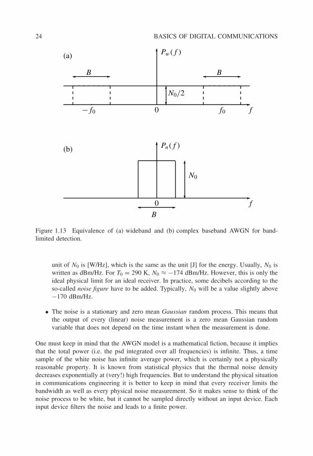
• The noise is white, that is, it has a constant power spectral density (psd). The one-sided psd is usually denoted by N0, so N0/2 is the two-sided psd, and BN0 is the noiseinside the (noise) bandwidth B, see part (a) of Figure 1.13. For thermal resistor noise,N0 = kT0, where k is the Boltzmann constant and T0 is the absolute temperature. The


�

�

�

�

� �

� ��

�

�

�

�f0

0 f

f0

(a)

(b)

−f0

Pw(f )

Pn(f )

N0

N0/2

B

B B

Figure 1.13 Equivalence of (a) wideband and (b) complex baseband AWGN for band-limited detection.

unit of N0 is [W/Hz], which is the same as the unit [J] for the energy. Usually, N0 iswritten as dBm/Hz. For T0 = 290 K, N0 ≈ −174 dBm/Hz. However, this is only theideal physical limit for an ideal receiver. In practice, some decibels according to theso-called noise figure have to be added. Typically, N0 will be a value slightly above−170 dBm/Hz.

• The noise is a stationary and zero mean Gaussian random process. This means thatthe output of every (linear) noise measurement is a zero mean Gaussian randomvariable that does not depend on the time instant when the measurement is done.

One must keep in mind that the AWGN model is a mathematical fiction, because it impliesthat the total power (i.e. the psd integrated over all frequencies) is infinite. Thus, a timesample of the white noise has infinite average power, which is certainly not a physicallyreasonable property. It is known from statistical physics that the thermal noise densitydecreases exponentially at (very!) high frequencies. But to understand the physical situationin communications engineering it is better to keep in mind that every receiver limits thebandwidth as well as every physical noise measurement. So it makes sense to think of thenoise process to be white, but it cannot be sampled directly without an input device. Eachinput device filters the noise and leads to a finite power.


1.3.1 Mathematical wideband AWGN

The mathematical AWGN random process w(t) can be characterized as a zero mean Gaus-sian process with the autocorrelation function

E{w(t1)w(t2)} = N0

2δ(t1 − t2). (1.48)

We see that for t1 = t2, this expression is not well defined, because δ(t) is not well definedfor t = 0. As for the δ-impulse, we must understand white noise as a generalized functionthat cannot be sampled directly, but it can be measured by a proper set of linear detectors.These linear detectors are the sampled outputs of linear filters. Thus, formally we can writethe output of the detector for the (real) signal φ(t) of such a white noise measurement asDφ[w] = [φ(−t) ∗ w(t)]t=0 or

Dφ[w] =∫ ∞

−∞φ(t)w(t) dt, (1.49)

that is, φ(−t) is the impulse response of the measuring device. In the mathematical litera-ture, φ(t) is called a test function (Reed and Simon 1980). Note that the integral in Equation(1.49) formally looks like the scalar product 〈φ, w〉. Keeping in mind that the scalar productis well defined only for finite-energy signals, we have avoided such a notation. We can nowcharacterize the white noise by the statistical properties of the outputs of linear detectors.

Definition 1.3.1 (White Gaussian Noise) White Gaussian noise w(t) is a random signal,characterized by the following properties: the output of a (finite-energy) linear detectorDφ[w] is a Gaussian random variable with zero mean. Any two detector outputs Dφ1 [w]and Dφ2 [w] are jointly Gaussian with cross-correlation

E{Dφ1 [w]Dφ2 [w]

} = N0

2〈φ1, φ2〉 . (1.50)

Since Gaussian random variables are completely characterized by their second-orderproperties (Papoulis 1991), all the statistical properties of w(t) are fixed by this definition.Using the integral representation (1.49), it is easy to show that the characterization bydetector outputs (1.50) is equivalent to (1.48) (see Problem 5).

Note that the AWGN outputs of orthogonal detectors are uncorrelated and thus, asGaussian random variables, even statistically independent. In many transmission setups asdiscussed in the above examples, the transmission base and therefore the correspondingdetectors are orthogonal. Thus, for an orthonormal transmission base, the detector outputsare both ISI-free and independent. Orthogonality thus means complete separability, whichwill lead us to the concept of sufficient statistics (see Subsection 1.4.1).

1.3.2 Complex baseband AWGN

Up to now, we have only considered wideband white Gaussian noise. The question now iswhat happens at the receiver when this additive disturbance of the useful signal is converted(together with the signal) to the complex baseband.


Consider a baseband detector for the real low-pass signal φ(t) and the detector thatcorresponds to the I-modulated version for the signal, φ = Iφ. We know from Equation(1.47) that the output of the detector for φ for any signal r is the same as the output of φ

for the I-demodulated version IDr of that signal. This same property also holds for whitenoise, that is, Dφ[w] = Dφ[IDw] . Similarly, for the Q-demodulated noise, we have the

property Dψ [w] = Dψ [QDw] with ψ = Qψ . Using this fact, together with the definitionof AWGN and Theorem 1.2.2, we get the following Proposition.

Proposition 1.3.2 Let w(t) be additive white Gaussian noise and its I- and Q-demodulatedversions be denoted by IDw and QDw. Let φ1 and φ2 be two strictly band-limited low-passdetectors. Then, the following properties hold:

E{Dφ1 [IDw]Dφ2 [IDw]

} = N0

2〈φ1, φ2〉 (1.51)

E{Dφ1 [QDw]Dφ2 [QDw]

} = N0

2〈φ1, φ2〉 (1.52)

E{Dφ1 [IDw]Dφ2 [QDw]

} = 0. (1.53)

The last equation means that the I- and the Q-demodulator produce statistically inde-pendent outputs2. Since both demodulators include a low-pass filter, both IDw and QDw

are well-behaved random processes having finite average power BN0/2. The samples (withsampling frequency B) of the low-pass white noise are given by the outputs of the detec-tor corresponding to (t), the impulse response of the ideal low-pass filter of bandwidthB/2. Thus, the low-pass white noise can be characterized by its detector outputs and by itssamples as well.

We now define the complex baseband noise process n(t) as the IQ-demodulated whitenoise

n = (ID + jQD)w. (1.54)

From the above proposition, we conclude

E{Dφ1 [n]D∗φ2

[n]} = N0 〈φ1, φ2〉 (1.55)

andE{Dφ1 [n]Dφ2 [n]} = 0. (1.56)

Complex random variables are characterized by these two types of covariances. Here thesecond one, the so-called pseudocovariance, has vanished. Gaussian processes with thisproperty are called proper Gaussian. Nonproper Gaussian random variables have undesiredproperties for describing communication systems (Neeser and Massey 1993). The autocor-relation properties of n(t) can simply be obtained by setting φ1(t) = t1(t) = (t − t1)

and φ2(t) = t2(t) = (t − t2), where (t) is the impulse response of the ideal low-pass filter of bandwidth B/2. Using

⟨t1 , t2

⟩ = (t1 − t2) we easily derive the followingproperties

E{n(t1) n∗(t2)} = N0(t1 − t2) (1.57)

2Equivalently, we may say that the I- and the Q-component of the noise are statistically independent.


and

E{n(t1) n(t2)} = 0. (1.58)

n(t) has similar properties as w(t). It is white, but restricted to a bandwidth B, and theconstant psd is N0 instead of N0/2. This can be understood because n(t) is complex andthe total power is the sum of the powers of the real and the imaginary part. Passband andcomplex baseband white noise psd is depicted in Figure 1.13.

Instead of dealing with complex white Gaussian noise with psd N0 band-limited to B/2,many authors regard it as convenient to perform the limit B → ∞, so that Equation (1.57)turns into

E{n(t1) n∗(t2)} = N0δ(t1 − t2),

that is, n(t) becomes complex infinite-bandwidth white noise with one- sided psd N0 (seee.g. (Kammeyer 2004; Proakis 2001)). This is reasonable if we think of downconvertingwith a low-pass filter of bandwidth much larger than the signal bandwidth. We wish to pointout that the limit B → ∞, that is, the wideband complex white noise does not reflect thephysical reality but is only a mathematically convenient model. The equivalence betweenpassband and baseband is only true for band-limited signals, especially B/2 < f0 musthold.

Proposition 1.3.3 (Baseband stochastic processes) Consider a (real-valued) stochasticprocess z(t) that influences the useful signal in the air. We want to characterize the IQ-demodulator output

z(t) = (t) ∗[√

2 exp (−j2πf0t) z(t)]

by its second-order properties, that is, an autocorrelation function. Here (t) = B sinc (Bt)

is the impulse response of the ideal low-pass filter of bandwidth B/2. We may think of whitenoise w(t) as such a process, but also of an RF carrier that is broadened by the Dopplereffect in a mobile radio environment (see Chapter 2). The following treatment is very general.We only assume that the random RF signal z(t) has zero mean and it is wide-sense stationary(WSS), which means that the autocorrelation function

R(τ ) = E {z(t + τ )z(t)}

of the process does not depend on t . We want to show that

E{z(t + τ )z∗(t)

} = (τ) ∗[2 exp (−j2πf0τ ) R(τ )

](1.59)

and

E {z(t + τ )z(t)} = 0. (1.60)

Obviously, for the special case of AWGN, this property is just given by the two Equations(1.57, 1.58) above.


To prove Equation (1.59), we apply the convolution in the definition of z(t)

E{z(t + τ )z∗(t)

}= 2 E

{∫ ∞

−∞dt1(t + τ − t1)e

−j2πf0t1 z(t1)

∫ ∞

−∞dt2(t − t2)e

j2πf0t2 z(t2)

}

= 2 E

{∫ ∞

−∞dt1

∫ ∞

−∞dt2(t + τ − t1)(t − t2)e

−j2πf0(t1−t2)R(t1 − t2)

}

= 2 E

{∫ ∞

−∞dt1

∫ ∞

−∞dt2

∫ ∞

−∞df (t + τ − t1)(t − t2)e

j2π(f −f0)(t1−t2)S(f )

},

where we have expressed R(τ ) by means of its Fourier transform, that is, the power spectraldensity S(f ) of the process. We have used the simpler notation

∫dx∫

dyf (x, y) instead of∫ (∫f (x, y) dy

)dx. Substituting the time integration variables according to t ′1 = t + τ − t1

and t ′2 = t − t2 and noting that t1 − t2 = τ − t ′1 + t ′2, we get the expression

2 E

{∫ ∞

−∞df S(f )

∫ ∞

−∞dt ′1(t ′1)e

j2π(f −f0)(τ−t ′1)

∫ ∞

−∞dt ′2(t ′2)e

+j2π(f −f0)t ′2}

= 2 E

{∫ ∞

−∞df ej2π(f −f0)τ S(f ) �

(f − f0

B

)}

= 2 E

{∫ ∞

−∞df ej2πf τ S(f + f0) �

(f

B

)},

which completes the proof. We note that

S(f ) = 2 S(f + f0) �

(f

B

),

the power spectral density of the process in the complex baseband, is the Fourier transformof the complex baseband autocorrelation function

R(τ ) = (τ) ∗[2 exp (−j2πf0τ ) R(τ )

].

The proof of Equation (1.60) is similar. Applying again the convolution in the definitionof z(t) leads to

E {z(t + τ )z(t)}

= 2 E

{∫ ∞

−∞dt1(t + τ − t1)e

−j2πf0t1 z(t1)

∫ ∞

−∞dt2(t − t2)e

−j2πf0t2 z(t2)

}

= 2 E

{∫ ∞

−∞dt1

∫ ∞

−∞dt2(t + τ − t1)(t − t2)e

−j2πf0(t1+t2)R(t1 − t2)

}

= 2 E

{∫ ∞

−∞dt1

∫ ∞

−∞dt2

∫ ∞

−∞df (t + τ − t1)(t − t2)e

−j2πf0(t1+t2)ej2πf (t1−t2)S(f )

}.


We now substitute the time integration variables according to t ′1 = t + τ − t1 and t ′2 = t − t2and get the expression

2 E

{∫ ∞

−∞df S(f )

∫ ∞

−∞dt ′1(t ′1)e

j2π(f −f0)(t+τ−t ′1)

∫ ∞

−∞dt ′2(t ′2)e

−j2π(f +f0)(t ′2−t)

}

= 2 E

{∫ ∞

−∞df S(f ) ej2π(f −f0)(t+τ) �

(f − f0

B

)ej2π(f +f0)t �

(f + f0

B

)}.

We note that

�

(f − f0

B

)�

(f + f0

B

)= 0,

which completes the proof.

1.3.3 The discrete AWGN channel

Consider a complex baseband signal s(t) band limited to B/2 to be transmitted at the carrierfrequency f0. The corresponding passband transmit signal s(t) given by Equation (1.34) iscorrupted by AWGN, resulting in the receive signal

r(t) = s(t) + w(t).

The IQ-demodulated complex baseband receive signal is then given by

r(t) = s(t) + n(t), (1.61)

where n(t) is complex baseband AWGN as introduced in the preceding subsection. Let{gk(t)}Kk=1 be an orthogonal transmit base, for example, a Nyquist base, and

s(t) =K∑

k=1

skgk(t). (1.62)

Let nk = Dgk[n] be the detector outputs of the noise for the detector gk(t). The detector

outputs at the receiver rk = Dgk[r] are then given by

rk = sk + nk. (1.63)

We conclude from Equations (1.55) and (1.56) that nk is discrete complex AWGN charac-terized by

E{ni n∗k} = N0δik (1.64)

andE{ni nk} = 0. (1.65)

For nk = xk + j yk, these two equations are equivalent to

E{xi xk} = N0

2δik, (1.66)

E{yi yk} = N0

2δik, (1.67)


andE{xi yk} = 0. (1.68)

The random variables xk have the joint pdf

p(x1, . . . , xK) = 1√

2πσ 2K

exp

(− 1

2σ 2

(x2

1 + · · · + x2K

))

for σ 2 = N0/2. The random variables yk have the same pdf. Defining the vectors

x = (x1, . . . , xK)T , y = (y1, . . . , yK)T

results in

p(x) = 1√

2πσ 2K

exp

(− 1

2σ 2‖x‖2

),

p(y) = 1√

2πσ 2K

exp

(− 1

2σ 2‖y‖2

).

The joint pdf for the xk, yk is the product of both. We define the complex noise vector

n = (n1, . . . , nK)T ,

and write, with p(n) = p(x, y) = p(x)p(y),

p(n) = 1√

2πσ 22K

exp

(− 1

2σ 2‖n‖2

).

Using the vector notation s = (s1, . . . , sK)T and r = (r1, . . . , rK)T for the transmit symbolsand the detector outputs, we write the discrete AWGN transmission channel (1.63) as

r = s + n. (1.69)

If the symbols sk are real numbers, one can depict this as a transmission mission of a vectorin the K-dimensional real Euclidean space with the canonical base e1 = (1, 0, 0, . . . , 0)T ,e2 = (0, 1, 0, . . . , 0)T , . . . . For complex sk, one may think of a 2K-dimensional real Eu-clidean space, because it has the same distance structure as a K-dimensional complexspace.

We have assumed that the transmit base is orthonormal. This is not a fundamentalrestriction, because one can always perform a base transform to an orthonormal base. Inthat case, the symbols si are related to the original transmit symbols xk by a transforms = Bx, where B is the matrix that describes the coordinate transform.

1.4 Detection of Signals in Noise

1.4.1 Sufficient statistics

For the sake of simplicity, consider the model of Equations (1.63) and (1.69) for onlythree real dimensions as illustrated in Figure 1.14. Assume that two real symbols s1, s2


Dimension 3

Dimensions 1 and 2

r

s

n

(r1, r2)

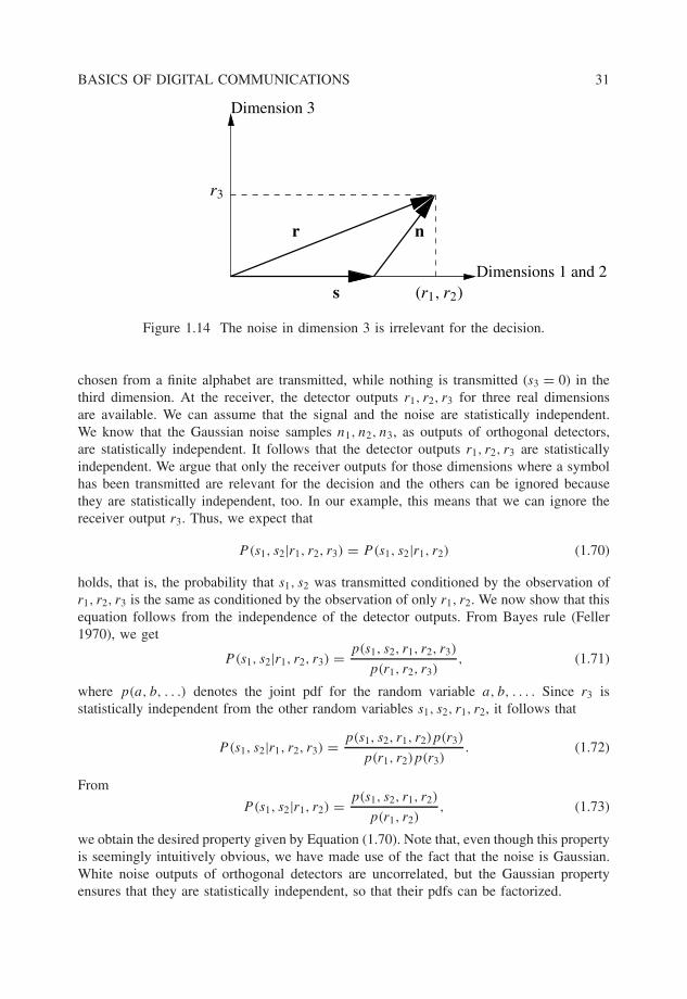
r3

Figure 1.14 The noise in dimension 3 is irrelevant for the decision.

chosen from a finite alphabet are transmitted, while nothing is transmitted (s3 = 0) in thethird dimension. At the receiver, the detector outputs r1, r2, r3 for three real dimensionsare available. We can assume that the signal and the noise are statistically independent.We know that the Gaussian noise samples n1, n2, n3, as outputs of orthogonal detectors,are statistically independent. It follows that the detector outputs r1, r2, r3 are statisticallyindependent. We argue that only the receiver outputs for those dimensions where a symbolhas been transmitted are relevant for the decision and the others can be ignored becausethey are statistically independent, too. In our example, this means that we can ignore thereceiver output r3. Thus, we expect that

P (s1, s2|r1, r2, r3) = P (s1, s2|r1, r2) (1.70)

holds, that is, the probability that s1, s2 was transmitted conditioned by the observation ofr1, r2, r3 is the same as conditioned by the observation of only r1, r2. We now show that thisequation follows from the independence of the detector outputs. From Bayes rule (Feller1970), we get

P (s1, s2|r1, r2, r3) = p(s1, s2, r1, r2, r3)

p(r1, r2, r3), (1.71)

where p(a, b, . . .) denotes the joint pdf for the random variable a, b, . . . . Since r3 isstatistically independent from the other random variables s1, s2, r1, r2, it follows that

P (s1, s2|r1, r2, r3) = p(s1, s2, r1, r2)p(r3)

p(r1, r2)p(r3). (1.72)

From

P (s1, s2|r1, r2) = p(s1, s2, r1, r2)

p(r1, r2), (1.73)

we obtain the desired property given by Equation (1.70). Note that, even though this propertyis seemingly intuitively obvious, we have made use of the fact that the noise is Gaussian.White noise outputs of orthogonal detectors are uncorrelated, but the Gaussian propertyensures that they are statistically independent, so that their pdfs can be factorized.


The above argument can obviously be generalized to more dimensions. We only needto detect in those dimensions where the signal has been transmitted. The correspondingdetector outputs are then called a set of sufficient statistics. For a more detailed discussion,see (Benedetto and Biglieri 1999; Blahut 1990; Wozencraft and Jacobs 1965).

1.4.2 Maximum likelihood sequence estimation

Again we consider the discrete-time model of Equations (1.63) and (1.69) and assume afinite alphabet for the transmit symbols sk , so that there is a finite set of possible transmitvectors s. Given a receive vector r, we ask for the most probable transmit vector s, that is,the one for which the conditional probability P (s|r) that s was transmitted given that r hasbeen received becomes maximal. The estimate of the symbol is

s = arg maxs

P (s|r). (1.74)

From Bayes law, we haveP (s|r)p(r) = p(r|s)P (s), (1.75)

where p(r) is the pdf for the receive vector r, p(r|s) is the pdf for the receive vector rgiven a fixed transmit vector s, and P (s) is the a priori probability for s. We assume thatall transmit sequences have equal a priori probability. Then, from

p(r|s) ∝ exp

(− 1

2σ 2‖r − s‖2

), (1.76)

we conclude thats = arg min

s‖r − s‖2 . (1.77)

Thus, the most likely transmit vector minimizes the squared Euclidean distance. From

‖r − s‖2 = ‖r‖2 + ‖s‖2 − 2 {s†r

},

we obtain the alternative condition

s = arg maxs

( {

s†r}− 1

2‖s‖2

). (1.78)

The first (scalar product) term can be interpreted as a cross correlation between the transmitand the receive signal. The second term is half the signal energy. Thus, the most likelytransmit signal is the one that maximizes the cross correlation with the receive signal,thereby taking into account a correction term for the energy. If all transmit signals havethe same energy, this term can be ignored.

The receiver technique described above, which finds the most likely transmit vector, iscalled maximum likelihood sequence estimation (MLSE). It is of fundamental importancein communication theory, and we will often need it in the following chapters.

A continuous analog to Equation (1.78) can be established. We recall that the continuoustransmit signal s(t) and the components sk of the discrete transmit signal vector s are relatedby

s(t) =K∑

k=1

skgk(t),


and the continuous receive signal r(t) and the components rk of the discrete transmit signalvector r are related by

rk = Dgk[r] =

∫ ∞

−∞g∗

k (t)r(t) dt.

From these relations, we easily conclude that

s†r =∫ ∞

−∞s∗(t)r(t) dt

holds. Equation (1.78) is then equivalent to

s = arg maxs

( {Ds[r]} − 1

2‖s‖2

)(1.79)

for finding the maximum likelihood (ML) transmit signal s(t). In the first term of thisexpression,

Ds[r] =∫ ∞

−∞s∗(t)r(t) dt

means that the detector outputs (= sampled MF outputs) for all possible transmit signalss(t) must be taken. For all these signals, half of their energy

‖s‖2 =∫ ∞

−∞|s(t)|2 dt

must be subtracted from the real part of the detector output to obtain the likelihood of eachsignal.

Example 3 (Walsh Demodulator) Consider a transmission with four possible transmitvectors s1, s2, s3 and s4 given by the columns of the matrix

[s1, s2, s3, s4] =

1 1 1 11 −1 1 −11 1 −1 −11 −1 −1 1

,

each being transmitted with the same probability. This is just orthogonal Walsh modulationfor M = 4. We ask for the most probable transmit vector s on the condition that the vector r =(1.5, −0.8, 1.1, −0.2)T has been received. Since all transmit vectors have equal energy,the most probable transmit vector is the one that maximizes the scalar product with r. Wecalculated the scalar products as

s1 · r = 2.0, s2 · r = 3.2, s3 · r = 0.4, s4 · r = 1.4.

We conclude that s2 has most probably been transmitted.


1.4.3 Pairwise error probabilities

Consider again a discrete AWGN channel as given by Equation (1.69). We write

r = s + nc,

where nc is the complex AWGN vector. For the geometrical interpretation of the followingderivation of error probabilities, it is convenient to deal with real vectors instead of complexones. By defining

y =[ {r}

� {r}]

, x =[ {s}

� {s}]

,

and

n =[ {nc}

� {nc}]

,

we can investigate the equivalent discrete real AWGN channel

y = x + n. (1.80)

Consider the case that x has been transmitted, but the receiver decides for another symbolx. The probability for this event (excluding all other possibilities) is called the pairwiseerror probability (PEP) P (x �→ x). Define the decision variable

X = ‖y − x‖2 − ‖y − x‖2

as the difference of squared Euclidean distances. If X > 0, the receiver will take an erro-neous decision for x. Then, using simple vector algebra (see Problem 7), we obtain

X = 2

[(y − x + x

2

)(x − x)

].

The geometrical interpretation is depicted in Figure 1.15. The decision variable is (upto a factor) the projection of the difference between the receive vector y and the centerpoint 1

2 (x + x) between the two possible transmit vectors on the line between them. Thedecision threshold is a plane perpendicular to that line. Define d = 1

2 (x − x) as the differencevector between x and the center point, that is, d = ‖d‖ is the distance of the two possibletransmit signals from the threshold. Writing y = x + n and using x = 1

2 (x + x) − d, thescaled decision variable X = 1

4dX can be written as

X = (−d + n) · dd

.

It can easily be shown that

n = n · dd

,

the projection of the noise onto the relevant dimension, is a Gaussian random variablewith zero mean and variance σ 2 = N0/2 (see Problem 8). Since X = −d + n, the errorprobability is given by

P (X) > 0) = P (n > d).


x

x

n

d

Decision threshold

n

yX

Figure 1.15 Decision threshold.

This equals

P (n > d) = Q

(dσ

), (1.81)

where the Gaussian probability integral is defined by

Q(x) = 1√2π

∫ ∞

x

e− 12 ξ2

dξ

The Q-function defined above can be expressed by the complementary Gaussian errorfunction erfc(x) = 1 − erf(x), where erf(x) is the Gaussian error function, as

Q (x) = 1

2erfc

(x√2

). (1.82)

The pairwise error probability can then be expressed by

P (x �→ x) = 1

2erfc

(√1

4N0‖x − x‖2

). (1.83)

Since the norms of complex vectors and the equivalent real vectors are identical, we canalso write

P (s �→ s) = 1

2erfc

(√1

4N0‖s − s‖2

). (1.84)

For the continuous signal,

s(t) =K∑

k=1

skgk(t), (1.85)


this is equivalent to

P (s(t) �→ s(t)) = 1

2erfc

(√1

4N0

∫ ∞

−∞|s(t) − s(t)|2 dt

). (1.86)

It has been pointed out by Simon and Divsalar (Simon and Divsalar 1998) that, formany applications, the following polar representation of the complementary Gaussian errorfunction provides a simpler treatment of many problems, especially for fading channels.

Proposition 1.4.1 (Polar representation of the Gaussian erfc function)

1

2erfc(x) = 1

π

∫ π/2

0exp

(− x2

sin2 θ

)dθ. (1.87)

Proof. The idea of the proof is to view the one-dimensional problem of pairwise errorprobability as two-dimensional and introduce polar coordinates. AWGN is a Gaussian ran-dom variable with mean zero and variance σ 2 = 1. The probability that the random variableexceeds a positive real value, x, is given by the Gaussian probability integral

Q(x) =∫ ∞

x

1√2π

exp

(−1

2ξ 2)

dξ. (1.88)

This probability does not change if noise of the same variance is introduced in the seconddimension. The error threshold is now a straight line parallel to the axis of the seconddimension, and the probability is given by

Q(x) =∫ ∞

x

(∫ ∞

−∞

1

2πexp

(−1

2(ξ 2 + η2)

)dη

)dξ. (1.89)

This integral can be written in polar coordinates (r, φ) as

Q(x) =∫ π/2

−π/2

(∫ ∞

x/ cos φ

r

2πexp

(−1

2r2)

dr

)dφ. (1.90)

The integral over r can immediately be solved to give

Q(x) =∫ π/2

−π/2

1

2πexp

(−1

2

x2

cos2 φ

)dφ. (1.91)

A simple symmetry argument now leads to the desired form of 12 erfc(x) = Q(

√2x).

An upper bound of the erfc function can easily be obtained from this expression byupper bounding the integrand by its maximum value,

1

2erfc(x) ≤ 1

2e−x2

. (1.92)

Example 4 (PEP for Antipodal Modulation) Consider the case of only two possibletransmit signals s1(t) and s2(t) given by

s1,2(t) = ±√

ES g(t),


where g(t) is a pulse normalized to ‖g‖2 = 1, and ES is the energy of the transmittedsignal. To obtain the PEP, according to Equation (1.86), we calculate the squared Euclideandistance

‖s1 − s2‖2 =∫ ∞

−∞|s1(t) − s2(t)|2 dt

between two possible transmit signals s1(t) and s2(t) and obtain

‖s1 − s2‖2 =∥∥∥√Es g −

(−√

Es g)∥∥∥2 = 4ES.

The PEP is then given by Equation (1.86) as

P (s1(t) �→ s2(t)) = 1

2erfc

(√ES

N0

).

One can transmit one bit by selecting one of the two possible signals. Therefore, the energyper bit is given by Eb = ES leading to the PEP

P (s1(t) �→ s2(t)) = 1

2erfc

(√Eb

N0

).

Example 5 (PEP for Orthogonal Modulation) Consider an orthonormal transmit basegk(t), k = 1, . . . , M . We may think of the Walsh base or the Fourier base as an example,but any other choice is possible. Assume that one of the M possible signals

sk(t) =√

ES gk(t)

is transmitted, where ES is again the signal energy. In case of the Walsh base, this is justWalsh modulation. In case of the Fourier base, this is just (orthogonal) FSK (frequency shiftkeying). To obtain the PEP, we have to calculate the squared Euclidean distance

‖si − sk‖2 =∫ ∞

−∞|si(t) − sk(t)|2 dt

between two possible transmit signals si(t) and sk(t) with i �= k. Because the base is or-thonormal, we obtain

‖si − sk‖2 = ES ‖gi − gk‖2 = 2ES.

The PEP is then given by

P (si(t) �→ sk(t)) = 1

2erfc

(√ES

2N0

).

One can transmit log2(M) bits by selecting one of M possible signals. Therefore, the energyper bit is given by Eb = ES/ log2(M), leading to the PEP

P (si(t) �→ sk(t)) = 1

2erfc

(√log2(M)

Eb

2N0

).


Concerning the PEP, we see that for M = 2, orthogonal modulation is inferior comparedto antipodal modulation, but it is superior if more than two bits per signal are transmitted.The price for that robustness of high-level orthogonal modulation is that the number of therequired signal dimensions and thus the required bandwidth increases exponentially with thenumber of bits.

1.5 Linear Modulation Schemes

Consider some digital information that is given by a finite bit sequence. To transmit thisinformation over a physical channel by a passband signal s(t) = {

s(t)ej2πf0t}, we need

a mapping rule between the set of bit sequences and the set of possible signals. We callsuch a mapping rule a digital modulation scheme. A linear digital modulation scheme ischaracterized by the complex baseband signal

s(t) =K∑

k=1

skgk(t),

where the information is carried by the complex transmit symbols sk . The modulationscheme is called linear, because this is a linear mapping from the vector s = (s1, . . . , sK)T

of transmit symbols to the continuous transmit signal s(t). In the following subsections, wewill briefly discuss the most popular signal constellations for the modulation symbols sk thatare used to transmit information by choosing one of M possible points of that constellation.We assume that M is a power of two, so each complex symbol sk carries log2(M) bits of theinformation. Although it is possible to combine several symbols to a higher-dimensionalconstellation, the following discussion is restricted to the case where each symbol sk ismodulated separately by a tuple of m = log2(M) bits. The rule how this is done is calledthe symbol mapping and the corresponding device is called the symbol mapper. In thissection, we always deal with orthonormal base pulses gk(t). Then, as discussed in thepreceding sections, we can restrict ourselves to a discrete-time transmission setup wherethe complex modulation symbols

sk = xk + jyk

are corrupted by complex discrete-time white Gaussian noise nk .

1.5.1 Signal-to-noise ratio and power efficiency

Since we have assumed orthonormal transmit pulses gk(t), the corresponding detector out-puts are given by

rk = sk + nk,

where nk is discrete complex AWGN. We note that, because the pulses are normalizedaccording to ∫ ∞

−∞g∗

i (t)gk(t) dt = δik,

the detector changes the dimension of the signal; the squared continuous signals have thedimension of a power, but the squared discrete detector output signals have the dimensionof an energy.


The average signal energy is given by

E = E

{∫ ∞

−∞|s(t)|2 dt

}= E

{K∑

k=1

|sk|2}

= K E{|sk|2

},

where we have assumed that all the K symbols sk have identical statistical properties. Theenergy per symbol ES = E/K is given by

ES = E{|sk|2

}.

The energy of the detector output of the noise is

EN = E{|nk|2

} = N0,

so the signal-to-noise ratio, SNR, defined as the ratio between the signal energy and therelevant noise, results in

SNR = ES

N0.

When thinking of practical receivers, it may be confusing that a detector changes thedimension of the signal, because we have interpreted it as a matched filter together witha sampling device. To avoid this confusion, we may introduce a proper constant. Forsignaling with the Nyquist base, gk(t) = g(t − kTS), one symbol sk is transmitted in eachtime interval of length TS . We then define the matched filter by its impulse response

h(t) = 1√TS

g∗(−t)

so that the matched filter output h(t) ∗ r(t) has the same dimension as the input signal r(t).The samples of the matched filter output are given by

1√TS

rk = 1√TS

sk + 1√TS

nk.

Then, the power of the sampled useful signal is given by

PS = E

{∣∣∣∣ 1√TS

sk

∣∣∣∣2}

= ES

TS

,

and the noise power is

PN = E

{∣∣∣∣ 1√TS

nk

∣∣∣∣2}

= N0

TS

.

Thus, the SNR may equivalently be defined as

SNR = PS

PN

,

which is the more natural definition for practical measurements.The SNR is a physical quantity that can easily be measured, but it does not say any-

thing about the power efficiency. To evaluate the power efficiency, one must know the


average energy Eb per useful bit at the receiver that is needed for a reliable recovery ofthe information. If log2(M) useful bits are transmitted by each symbol sk, the relation

ES = log2(M) Eb

holds, which relates both quantities by

SNR = log2(M)Eb

N0.

We note the important fact that Eb = PS/Rb is just the average signal power PS neededper useful bit rate Rb. Therefore, a modulation that needs less Eb/N0 to achieve a reliabletransmission is more power efficient .

In the following sections, we discuss the most popular symbol mappings and theirproperties.

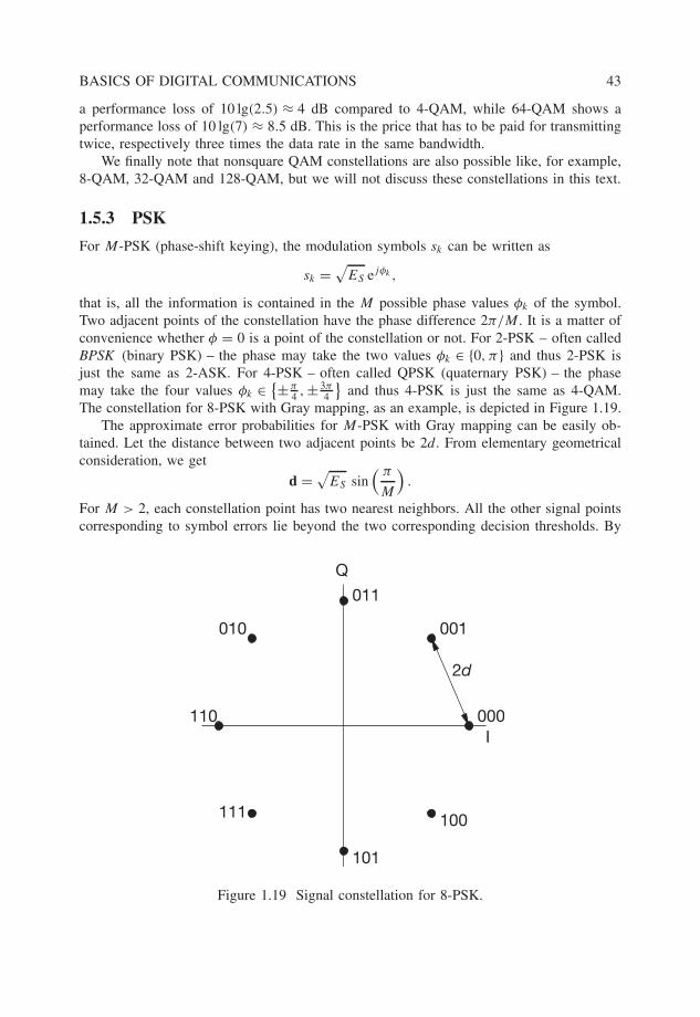
1.5.2 ASK and QAM

For M-ASK (amplitude-shift keying), a tuple of m = log2(M) bits will be mapped onlyon the real part xk of sk , while the imaginary part yk will be set to zero. The M pointswill be placed equidistant and symmetrically about zero. Denoting the distance betweentwo points by 2d, the signal constellation for 2-ASK is given by xl ∈ {±d}, for 4-ASK byxl ∈ {±d, ±3d} and for 8-ASK by xl ∈ {±d, ±3d, ±5d, ±7d} . We consider Gray mapping,that is, two neighboring points differ only in one bit. In Figure 1.16, the M-ASK signalconstellations are depicted for M = 2, 4, 8.

Assuming the same a priori probability for each signal point, we easily calculate thesymbol energies as ES = E

{|sk|2} = d2, 5d2, 21d2 for these constellations, leading to the

respective energies per bit Eb = ES/ log2(M) = d2, 2.5d2, 7d2.Adjacent points have the distance 2d, so the distance to the corresponding decision

threshold is given by d. If a certain point of the constellation is transmitted, the probabilitythat an error occurs because the discrete noise with variance σ 2 = N0/2 (per real dimension)exceeds the distance to the decision threshold with distance d is given by

Perr = Q

(dσ

)= 1

2erfc

√

d2

N0

, (1.93)

01

00011110

010 011 001 000

0 +d–7d –5d –3d –d +3d +5d +7d

111101100 110

Figure 1.16 M-ASK Constellation for M = 2, 4, 8.


see Equation (1.81). For the two outer points of the constellation, this is just the probabilitythat a symbol error occurs. In contrast, for M > 2, each inner point has two neighbors,leading to a symbol error probability of 2Perr for these points. Averaging over the symbolerror probabilities for all points of each constellation, we get the symbol error probabilities

P 2−ASKS = Q

(dσ

), P 4−ASK

S = 3

2Q

(dσ

), P 8−ASK

S = 7

4Q

(dσ

).

For Gray mapping, we can make the approximation that each symbol error leads only toone bit error. Thus, we readily obtain the bit error probabilities expressed by the bit energyfor M = 2, 4, 8 as

P 2−ASKb = 1

2erfc

(√Eb

N0

),

and

P 4−ASKb ≈ 3

8erfc

(√2

5

Eb

N0

), (1.94)

P 8−ASKb ≈ 7

24erfc

(√1

7

Eb

N0

).

For ASK constellations, only the I-component, corresponding to the cosine wave, willbe modulated, while the sine wave will not be present in the passband signal. Since, ingeneral, every passband signal of a certain bandwidth may have both components, 50% ofthe bandwidth resources remain unused. A simple way to use these resources is to applythe same ASK modulation for the Q-component too. We thus have complex modulationsymbols sk = xk + jyk , where both xk and yk are taken from an M-ASK constellation. Theresult is a square constellation of M2 signal points in the complex plane, as depicted inFigure 1.17 for M2 = 64. We call this an M2-QAM (quadrature amplitude modulation).The bit error performance of M2-QAM as a function of Eb/N0 is the same as for M-ASK,that is,

P4−QAMb = 1

2erfc

(√Eb

N0

),

P16−QAMb ≈ 3

8erfc

(√2

5

Eb

N0

)(1.95)

and

P64−QAMb ≈ 7

24erfc

(√1

7

Eb

N0

).

This is because the I- and the Q-component can be regarded as completely independentchannels that do not influence each other. Thus, M2-QAM can be regarded as M-ASKmultiplexed to the orthogonal I- and Q-channel. Note that the bit error rates are not identicalif they are plotted as a function of the signal-to-noise ratio. The bit error probabilities ofEquations (1.95) are depicted in Figure 1.18. For high values of Eb/N0, 16-QAM shows


Q

I

Figure 1.17 The 64-QAM constellation.

0 5 10 15 2010–6

10–5

10–4

10–3

10–2

10–1

100

Eb/N0 [dB]

Pb

4-QAM 16-QAM 64-QAM

Figure 1.18 Bit error probabilities for 4-QAM, 16-QAM, and 64-QAM.


a performance loss of 10 lg(2.5) ≈ 4 dB compared to 4-QAM, while 64-QAM shows aperformance loss of 10 lg(7) ≈ 8.5 dB. This is the price that has to be paid for transmittingtwice, respectively three times the data rate in the same bandwidth.

We finally note that nonsquare QAM constellations are also possible like, for example,8-QAM, 32-QAM and 128-QAM, but we will not discuss these constellations in this text.

1.5.3 PSK

For M-PSK (phase-shift keying), the modulation symbols sk can be written as

sk =√

ES ejφk ,

that is, all the information is contained in the M possible phase values φk of the symbol.Two adjacent points of the constellation have the phase difference 2π/M . It is a matter ofconvenience whether φ = 0 is a point of the constellation or not. For 2-PSK – often calledBPSK (binary PSK) – the phase may take the two values φk ∈ {0, π} and thus 2-PSK isjust the same as 2-ASK. For 4-PSK – often called QPSK (quaternary PSK) – the phasemay take the four values φk ∈ {±π

4 , ± 3π4

}and thus 4-PSK is just the same as 4-QAM.

The constellation for 8-PSK with Gray mapping, as an example, is depicted in Figure 1.19.The approximate error probabilities for M-PSK with Gray mapping can be easily ob-

tained. Let the distance between two adjacent points be 2d. From elementary geometricalconsideration, we get

d =√

ES sin( π

M

).

For M > 2, each constellation point has two nearest neighbors. All the other signal pointscorresponding to symbol errors lie beyond the two corresponding decision thresholds. By

000

001010

110

111 100

I

Q

2d

101

011

Figure 1.19 Signal constellation for 8-PSK.


a simple union-bound argument, we find that the symbol error probability can be tightlyupper bounded by

PS ≤ 2Q

(dσ

)= erfc

(√sin2

( π

M

) ES

N0

).

By assuming that only one bit error occurs for each symbol error and taking into accountthe relation ES = log2(M) Eb, we get the approximate expression

Pb ≈ 1

log2(M)erfc

(√log2(M) sin2

( π

M

) Eb

N0

)(1.96)

for the bit error probability. The bit error probabilities of Equation (1.96) are de-picted in Figure 1.20. For high values of Eb/N0, 8-PSK shows a performance loss of10 lg(3 sin2(π/8)) ≈ 3.6 dB compared to 4-PSK, while 16-PSK shows a performance lossof 10 lg(4 sin2(π/16)) ≈ 8.2 dB. Thus, higher-level PSK modulation leads to a considerableloss in power efficiency compared to higher-level QAM at the same spectral efficiency.

1.5.4 DPSK

For DPSK (differential PSK), the phase difference between two adjacent transmit symbolscarries the information, not the phase of the transmit symbol itself. This means that for asequence of transmit symbols

sk =√

ES ejφk ,

0 5 10 15 2010–6

10–5

10–4

10–3

10–2

10–1

100

Eb/N0 [dB]

Pb

4-PSK 8-PSK 16-PSK

Figure 1.20 Bit error probabilities for 4-PSK, 8-PSK and 16-PSK.


the information is carried by�φk = φk − φk−1,

andzk = ej�φk

is a symbol taken from an M-PSK constellation with energy one. The transmit symbols arethen given by the recursion

sk = zk · sk−1

with a start symbol s0 that may have some arbitrary reference phase φ0. We may set thisphase equal to zero and write

s0 =√

ES.

Because of this phase reference symbol, the transmit signal

s(t) =K∑

k=0

skgk(t)

carries K + 1 transmit symbols sk, but only K useful PSK symbols zk . Typically, the phasereference symbol will be transmitted at the beginning of a frame, and the frame length islarge enough so that the loss in data rate due to the reference symbol can be neglected.

Again it is a matter of convenience whether the PSK constellation for zk containsthe phase (difference) �φk = 0 or not. For the most popular QPSK constellation, �φk ∈{±π

4 , ± 3π4

}or

zk ∈{

1√2

(±1 ± j)

}.

Obviously, this leads to eight possible values of the transmit symbol sk, corresponding tothe absolute phase values

φk ∈{

0, ±π

4, ±π

2, ±3π

4, π

},

see Figure 1.21, where the possible transitions are marked by arrows.For even values of k,

φk ∈{

0, ±π

2, π}

and for odd values of k,

φk ∈{±π

4, ±3π

4

}.

We thus have two different constellations for sk, which are phase shifted by π/4. Thismodulation scheme is therefore called π/4-DQPSK.

Differential PSK is often used because it does not require an absolute phase reference.In practice, the channel introduces an unknown phase θ , that is, the receive signal is

rk = ejθ sk + nk.

In a coherent PSK receiver, the phase must be estimated and back- rotated. A differentialreceiver compares the phase of two adjacent symbols by calculating

uk = rkr∗k−1 = sks

∗k−1 + ejθ skn

∗k−1 + nke−jθ s∗

k−1 + nkn∗k−1.


I

Q

Figure 1.21 Transmit symbols for π4 -DQPSK.

In the noise-free case, uk/√

ES = zk represents original PSK symbols that carry the infor-mation. However, we see from the above equation that we have additional noise terms thatdo not occur for coherent signaling and that degrade the performance. The performanceanalysis of DPSK is more complicated than for coherent PSK (see e.g. (Proakis 2001)). Wewill later refer to the results when we need them for the applications.

1.6 Bibliographical Notes

This chapter is intended to give a brief overview of the basics that are needed in the follow-ing chapters and to introduce some concepts and notations. A more detailed introductioninto digital communication and detection theory can be found in many text books (see e.g.(Benedetto and Biglieri 1999; Blahut 1990; Kammeyer 2004; Lee and Messerschmidt 1994;Proakis 2001; Van Trees 1967; Wozencraft and Jacobs 1965)). We assume that the readeris familiar with Fourier theory and has some basic knowledge of probability and stochasticprocesses. We will not define these concepts further; one may refer to standard text books(see e.g. (Bracewell 2000; Feller 1970; Papoulis 1991)).

We have emphasized the vector space properties of signals. This allows a geometricalinterpretation that makes the solution of many detection problems intuitively obvious. Theinterpretation of signals as vectors is not new. We refer to the excellent classical text books(Van Trees 1967; Wozencraft and Jacobs 1965).

We have emphasized the concept of a detector as an integral operation that performs ameasurement. A Fourier analyzer is such a device that may be interpreted as a set of detec-tors, one for each frequency. The integral operation is given by a scalar product if the signal


is well behaved (i.e. of finite energy). If not, the signal has to be understood as a generalizedfunction (which is called distribution or functional in mathematical literature (Reed andSimon 1980)), and the detection is the action of this signal on a well-behaved test function.It is interesting to note that this is the same situation as in quantum theory, where such a testfunction is interpreted as a detection device for the quantum state of a physical system. Inthis context it is worth noting that δ(t), the most important generalized function in commu-nication theory, has been introduced by one of the quantum theory pioneers, P.A.M. Dirac.

1.7 Problems

1. Let {gk(t)}Kk=1 be an orthonormal transmit base and

s = (s1, . . . , sK)T

andx = (x1, . . . , xK)T

two transmit symbol vectors. Let

s(t) =K∑

k=1

skgk(t)

and

x(t) =K∑

k=1

xkgk(t).

Show that〈s, x〉 = s†x.

2. Let S(f ) denote the Fourier transform of the signal s(t) and define

s(t) =√

2 {s(t)ej2πf0t }.

Show that the Fourier transform of that signal is given by

S(f ) = 1√2

(S (f − f0) + S∗ (−f − f0)

).

3. Let x(t) and y(t) be finite-energy low-pass signals strictly band- limited to B/2and let f0 > B/2. Show that the two signals

x(t) =√

2 cos (2πf0t) x(t)

andy(t) = −

√2 sin (2πf0t) y(t)


are orthogonal. Let u(t) and v(t) be two other finite-energy signals strictly band-limited to B/2 and define

u(t) =√

2 cos (2πf0t) u(t)

andv(t) = −

√2 sin (2πf0t) v(t).

Show that〈u, x〉 = 〈u, x〉

and〈v, y〉 = 〈v, y〉

hold. Hint: Transform all the signals into the frequency domain and use Parseval’sequation.

4. Show that, from the definition of the time-variant linear systems I and Q, thedefinitions (given in Subsection 1.2.2) of the time-variant linear systems ID andQD are uniquely determined by

〈u, Iv〉 = ⟨IDu, v

⟩and

〈u, Qv〉 = ⟨QDu, v

⟩for any (real-valued) finite-energy signal u(t) and v(t). Mathematically speaking,this means that ID and QD are defined as the adjoints of the linear operators I

and Q. For the theory of linear operators, see for example (Reed and Simon 1980).

5. Show that the definitions

E {w(t1)w(t2)} = N0

2δ(t1 − t2)

and

E{Dφ1 [w]Dφ2 [w]

} = N0

2〈φ1, φ2〉

are equivalent conditions for the whiteness of the (real-valued) noise w(t).

6. Let g(t) be a transmit pulse and n(t) complex baseband white (not necessarilyGaussian) noise. Let

Dh[r] =∫ ∞

−∞h∗(t)r(t) dt

be a detector for a (finite-energy) pulse h(t) and r(t) = g(t) + n(t) be the transmitpulse corrupted by the noise. Show that the signal-to-noise ratio after the detectordefined by

SNR = |Dh[g]|2E{|Dh[n]|2}

becomes maximal if h(t) is chosen to be proportional to g(t).


7. Show the equality

‖y − x‖2 − ‖y − x‖2 = 2

[(y − x + x

2

)(x − x)

].

8. Let n = (n1, . . . , nK)T be a K-dimensional real-valued AWGN with variance σ 2 =N0/2 in each dimension and u = (u1, . . . , uK)T be a vector of length |u| = 1 inthe K-dimensional Euclidean space. Show that n = n · u is a Gaussian randomvariable with mean zero and variance σ 2 = N0/2.

9. We consider a digital data transmission from the Moon to the Earth. Assume thatthe digital modulation scheme (e.g. QPSK) requires Eb/N0 = 10 dB at the receiverfor a sufficiently low bit error rate of, for example, BER = 10−5. For free-spacepropagation, the power at the receiver is given by

Pr = GtGr

λ2

(4πR)2 Pt .

We assume Gt = Gr = 10 dB for the antenna gains at the receiver and the trans-mitter, respectively, and λ = 40 cm for the wavelength. The distance of the moonis approximately given by R = 400 000 km. The receiver noise (including a noisefigure of 4 dB) is given by N0 = −170 dBm/Hz. How much transmit power isnecessary for a bit rate of Rb = 1 bit/s?

Date post:	17-Mar-2022
Category:	Documents
Upload:	others
View:	3 times
Download:	0 times

Basics of Digital Communications

Documents