31
Basics on Digital Signal Processing z - transform - Digital Filters Vassilis Anastassopoulos Electronics Laboratory, Physics Department, University of Patras
| Date post: | 16-Apr-2018 |
| Category: |
Documents |
| Upload: | truongtruc |
| View: | 236 times |
| Download: | 9 times |

Basics on Digital Signal Processing
z - transform - Digital Filters
Vassilis Anastassopoulos
Electronics Laboratory, Physics Department,
University of Patras

2/31
Outline of the Lecture
1. The z-transform
2. Properties
3. Examples
4. Digital filters
5. Design of IIR and FIR filters
6. Linear phase

3/31
z-Transform
The z-transform is more general than the DFT
Time to frequency
1
0
2
)()(N
n
nkNj
enxkX
1
0
)()(N
n
nznxzX
Time to z-domain (complex)
Transformation tool is the
complex wave
With amplitude |ejω|=1
Nkjj ee /2
Transformation tool is
With amplitude ρ
changing(?) with time
jj eez
4/31
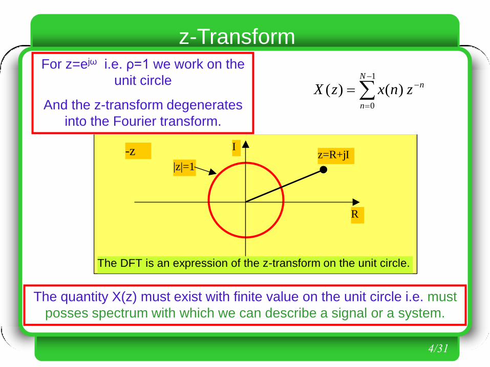
R
I z=R+jI -z
|z|=1
The DFT is an expression of the z-transform on the unit circle.
z-Transform For z=ejω i.e. ρ=1 we work on the
unit circle
And the z-transform degenerates
into the Fourier transform.
1
0
)()(N
n
nznxzX
The quantity X(z) must exist with finite value on the unit circle i.e. must
posses spectrum with which we can describe a signal or a system.

5/31
z-Transform convergence
We are interested in those values of z for which X(z) converges.
This region should contain the unit circle.
R
I
|a|
ROC
Why is it so?
The values of z for which X(z) diverges are
called poles of X(z).
1
0
1
0
)(1/ )( )()(N
n
nN
n
n znxznxzX
At z=0, X(z) diverges

6/31
R
I
|a|
ROC
a
a2
a3
a4
x(n)
n
1
z-Transform example
Which is the z-transform and the ROC of a discrete time sequence
x(n)=an for n0 and a<1 ?
0
1
0
1
0
)( )()(n
n
n
nnN
n
n azzaznxzX
which for |az-1|<1 or |z|>|a| converges to az
z
azzX
11
1)(
The pole z=a, is never included in the ROC

7/31
Poles and zeros of X(z)
R
I
|a|
ROC
Poles: X(z)= Zeros: X(z)=0
For finite sequences, X(z) converges
everywhere except at z=0
For infinite sequences, X(z) converges
everywhere outside the circle with radius the
pole with maximum value.
1
3
5
3
1
n
x(n)
X z x n z z z z z zn
n
( ) ( )
1 2 3 4 53 5 3
For stable, causal digital systems the region of convergence includes the
Unit Circle so that the system possesses spectrum
8/31
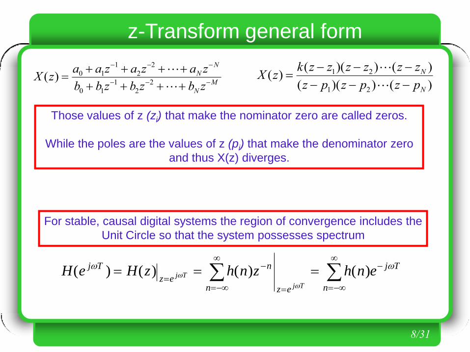
M
N
N
N
zbzbzbb
zazazaazX
2
2
1
10
2
2
1
10)(
z-Transform general form
Those values of z (zi) that make the nominator zero are called zeros.
While the poles are the values of z (pi) that make the denominator zero
and thus X(z) diverges.
)())((
)())(()(
21
21
N
N
pzpzpz
zzzzzzkzX
For stable, causal digital systems the region of convergence includes the
Unit Circle so that the system possesses spectrum
H e H z h n z h n ej T
z e
n
n z e
j T
n
j T
j T
( ) ( ) ( ) ( )
9/31
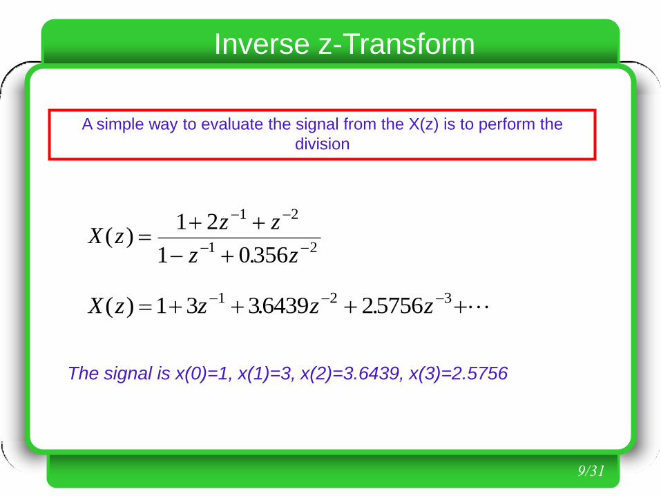
A simple way to evaluate the signal from the X(z) is to perform the
division
X zz z
z z( )
.
1 2
1 0356
1 2
1 2
X z z z z( ) . . 1 3 36439 257561 2 3
The signal is x(0)=1, x(1)=3, x(2)=3.6439, x(3)=2.5756
Inverse z-Transform
10/31
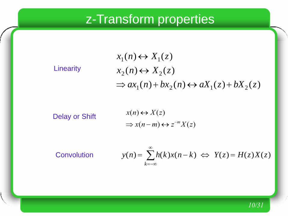
z-Transform properties
Delay or Shift )()(
)()(
zXzmnx
zXnx
m
x n X z
x n X z
ax n bx n aX z bX z
1 1
2 2
1 2 1 2
( ) ( )
( ) ( )
( ) ( ) ( ) ( )
Linearity
y n h k x n k Y z H z X zk
( ) ( ) ( ) ( ) ( ) ( )
Convolution

11/31
y(n-Μ)
x(n-Ν)
y(n-Μ+1)
x(n-Ν+1) x(n-2)
y(n-2) y(n-1)
x(n-1)
y(n)
x(n) Ts
Ts Ts Ts
b1
a1 a0
b2
a2 aΝ-1
bΜ-1 bΜ
aΝ
+
Ts Ts
z-Transform and digital systems
y n a x n k b y n kk
k
N
k
k
M
( ) ( ) ( )
0 1
N
k
k
k
N
k
k
k
zb
za
zH
1
0
1
)(
12/31
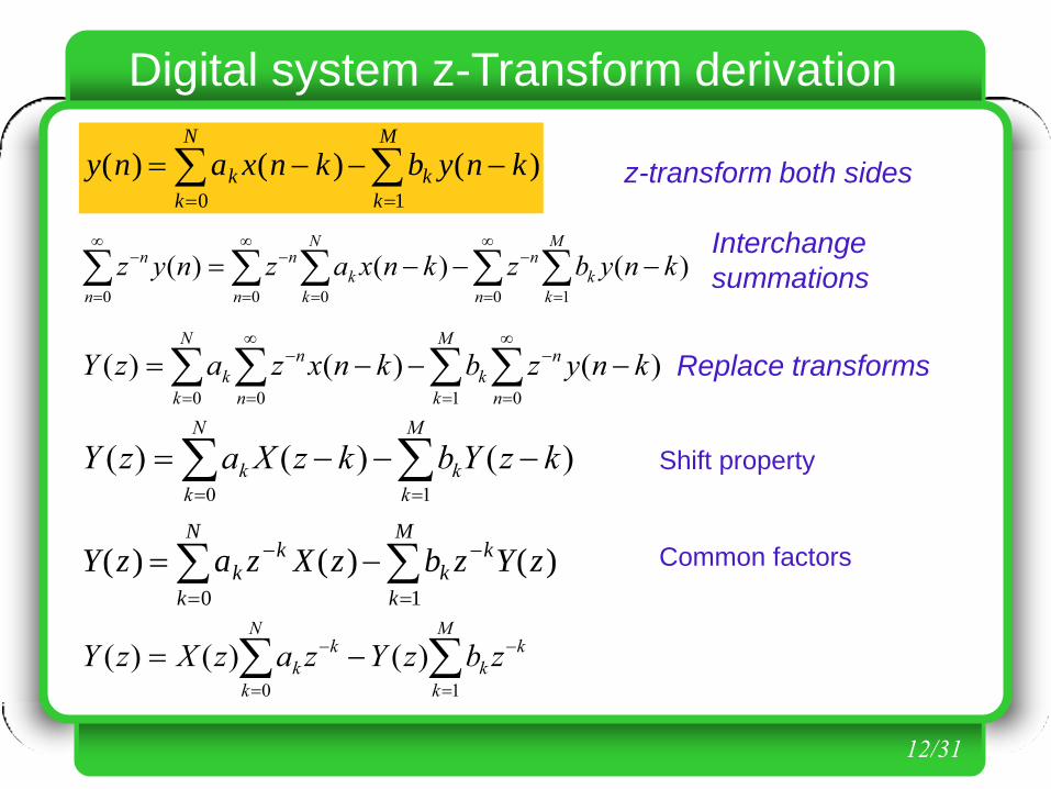
y n a x n k b y n kk
k
N
k
k
M
( ) ( ) ( )
0 1
Y z a z X z b z Y zkk
k
N
kk
k
M
( ) ( ) ( )
0 1
M
k
k
n
nN
k
k
n
n
n
n knybzknxaznyz10000
)()()(
0100
)()()(n
nM
k
k
n
nN
k
k knyzbknxzazY
M
k
k
N
k
k kzYbkzXazY10
)()()(
z-transform both sides
Replace transforms
Interchange
summations
Shift property
Digital system z-Transform derivation
Common factors
M
k
k
k
N
k
k
k zbzYzazXzY10
)()()(
13/31
Digital system z-Transform derivation
)(
1)(
)(
1
0 zH
zb
za
zX
zYN
k
k
k
N
k
k
k
N
k
k
k
M
k
k
k zazXzbzY01
)()1)((
Common factors
N
k
k
k
M
k
k
k zazXzbzYzY01
)()()(
y n a x n k b y n kk
k
N
k
k
M
( ) ( ) ( )
0 1
y(n-Μ)
x(n-Ν)
y(n-Μ+1)
x(n-Ν+1) x(n-2)
y(n-2) y(n-1)
x(n-1)
y(n)
x(n) Ts
Ts Ts Ts
b1
a1 a0
b2
a2 aΝ-1
bΜ-1 bΜ
aΝ
+
Ts Ts
Time
Frequency

14/31
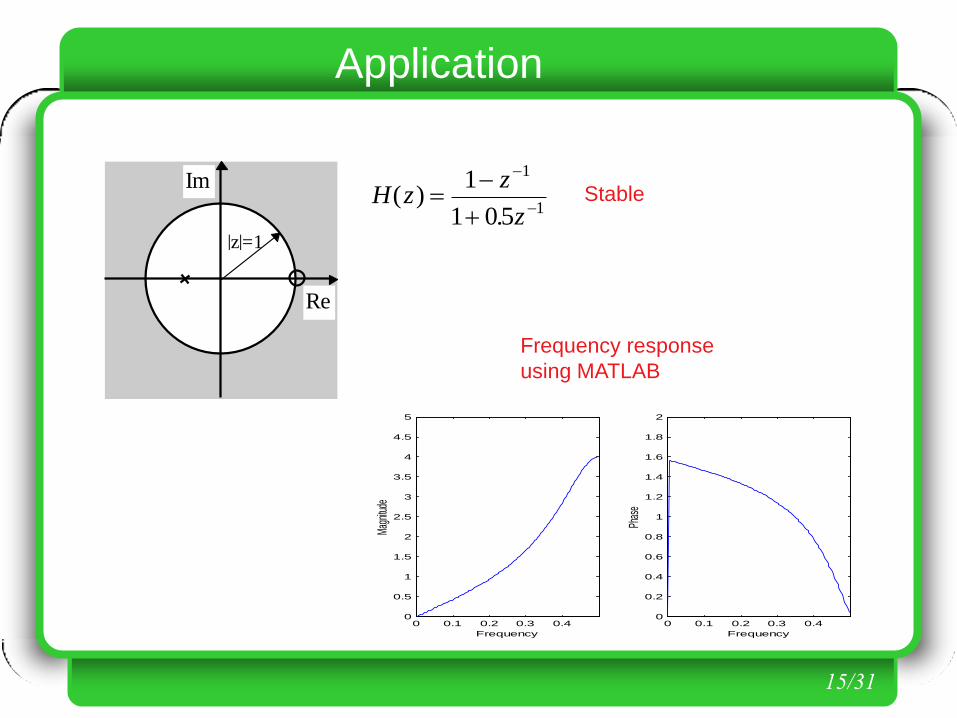
Application
Find the impulse response h(n) and the input-output relationship of the filter
described by H z
z
z( )
.
1
1 05
1
1
Examine the stability of the filter and find its frequency response.
H zY z
X z
z
z
Y z Y z z X z X z z
y n y n x n x n
y n x n x n y n
Z
( )( )
( ) .
( ) . ( ) ( ) ( )
( ) . ( ) ( ) ( )
( ) ( ) ( ) . ( )
1
1 0 5
0 5
0 5 1 1
1 0 5 1
1
1
1 11
Solution
y(n)
x(n)
z-1
z-1
-1
-0.5
( ) / ( . ) . . .1 1 05 1 15 0 75 03751 1 1 2 3 z z z z z
h(n) is obtained from the terms of the polynomial which results after the division
15/31
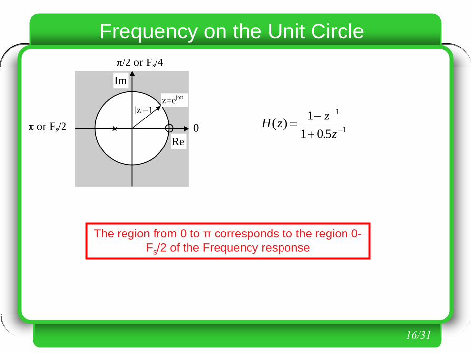
Application
Im
Re
|z|=1
1
H zz
z( )
.
1
1 05
1
1Stable
0 0.1 0.2 0.3 0.40
0.5
1
1.5
2
2.5
3
3.5
4
4.5
5
Frequency
Mag
nitud
e
0 0.1 0.2 0.3 0.40
0.2
0.4
0.6
0.8
1
1.2
1.4
1.6
1.8
2
FrequencyPh
ase
Frequency response
using MATLAB
16/31
Im
Re
|z|=1
0
π/2 or Fs/4
π or Fs/2
z=ejωt
H zz
z( )
.
1
1 05
1
1
The region from 0 to π corresponds to the region 0-
Fs/2 of the Frequency response
Frequency on the Unit Circle

17/31
Digital Filters
•They are characterized by their
Impulse Response h(n), their
Transfer Function H(z) and their
Frequency Response H(ω).
•They can have memory, high
accuracy and no drift with time and
temperature.
•They can possess linear phase.
•They can be implemented by digital
computers.

18/31
Digital Filters - Categories
IIR y n a k x n k b y n kk
N
k
k
M
( ) ( ) ( ) ( )
0 1
H z
a z
b z
kk
k
N
kk
k
M( )
0
1
1
y(n-Μ)
x(n-Ν)
y(n-Μ+1)
x(n-Ν+1) x(n-2)
y(n-2) y(n-1)
x(n-1)
y(n)
x(n) Ts
Ts Ts Ts
b1
a1 a0
b2
a2 aN-1
bΜ-1 bΜ
aN
+
Ts Ts

19/31
FIR
Digital Filters - Categories
y n h k x n k a k x n kk
N
k
N
( ) ( ) ( ) ( ) ( )
0 0
H z a z h k zkk
k
Nk
k
N
( ) ( )
0 0
x(n-Ν+1) x(n-Ν+2) x(n-2) x(n-1)
y(n)
x(n) Ts
aΝ-1 ή
h(Ν-1)
aΝ-2 ή
h(Ν-2) a2 ή
h(2)
a1 ή
h(1)
a0 ή
h(0)
+
Ts Ts
•Stable
•Linear phase

20/31
Digital Filters - Examples
0 0.1 0.2 0.3 0.40
0.5
1
1.5
Frequency
Ma
gnitud
e II
R0 0.1 0.2 0.3 0.4
-3
-2
-1
0
1
Frequency
Pha
se
IIR
0 0.1 0.2 0.3 0.40
0.5
1
1.5
Frequency
Ma
gnitud
e F
IR
0 0.1 0.2 0.3 0.4-4
-2
0
2
4
FrequencyP
ha
se
FIR
H za a z a z
b z b z( )
0 11
22
11
221
H z h k z k
k
( ) ( )
0
11
a0=0.498, a1=0.927,
a2=0.498, b1=-0.674
b2=-0.363.
h(1)=h(10)=-0.04506
h(2)=h(9)=0.06916
h(3)=h(8)=-0.0553
h(4)=h(7)=-.06342
h(5)=h(4)=0.5789

21/31
IIR filter design
Design using the Bilinear z-transform, BZT
Design using the position of poles and zeros
on the unit circle
Im
3Fs/4
Fs/4
-Fs/2
Fs/2 0 or Fs |z|=1
1
•The frequency response is zero at the
points of zeros
•The frequency response takes a peak at
the position of poles.
•In order to have real coefficients of the
filter, the poles must appear in pairs. The
same happens for the zeros as well.
22/31
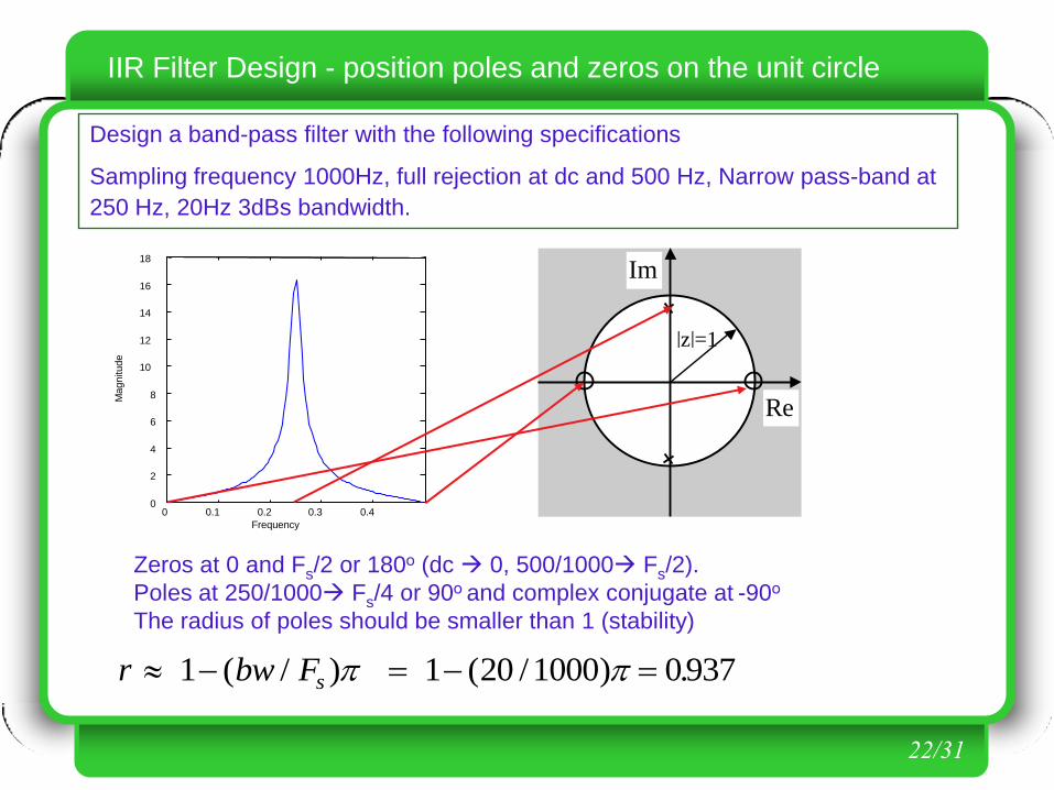
IIR Filter Design - position poles and zeros on the unit circle
Design a band-pass filter with the following specifications
Sampling frequency 1000Hz, full rejection at dc and 500 Hz, Narrow pass-band at
250 Hz, 20Hz 3dBs bandwidth.
0 0.1 0.2 0.3 0.4 0
2
4
6
8
10
12
14
16
18
Frequency
Magnitude
Zeros at 0 and Fs/2 or 180ο (dc 0, 500/1000 Fs/2).
Poles at 250/1000 Fs/4 or 90ο and complex conjugate at -90ο
The radius of poles should be smaller than 1 (stability)
r bw Fs 1 1 20 1000 0937( / ) ( / ) .
Im
Re
|z|=1
1

23/31
IIR Filter Design - position poles and zeros on the unit circle
y(n)
x(n)
0.87
z-2
z-2
Im
Re
|z|=1
1
H zz z
z re z re
z
z
z
zj j( )
( )( )
( )( ) . ./ /
1 1 1
0877969
1
1 08779692 2
2
2
2
2
937.0)1000/20(1 )/(1 sFbwr
0 0.1 0.2 0.3 0.40
2
4
6
8
10
12
14
16
18
Frequency
Magn
itude
0 0.1 0.2 0.3 0.4-2
-1.5
-1
-0.5
0
0.5
1
1.5
2
Frequency
Phas
e
y n x n x n y n( ) ( ) ( ) . ( ) 2 0877969 2

24/31
FIR filters
y n h k x n k a k x n kk
N
k
N
( ) ( ) ( ) ( ) ( )
0 0
H z a z h k zkk
k
Nk
k
N
( ) ( )
0 0
x(n-Ν+1) x(n-Ν+2) x(n-2) x(n-1)
y(n)
x(n) Ts
aΝ-1 ή
h(Ν-1)
aΝ-2 ή
h(Ν-2) a2 ή
h(2)
a1 ή
h(1)
a0 ή
h(0)
+
Ts Ts
•Stable
•Linear phase
Design Methods
• Optimal filters
• Windows method
• Sampling frequency

25/31
Main categories of ideal filters
0
0
1
|Η(ω)|
2π ωc π 0
1
|Η(ω)|
2π ωc1 ωc2 π 0
1
|Η(ω)|
2π ωc π
0
j
Η(ω)
2π π
-j
j Η(ω)
2π π
Low-pass Band-pass High-pass
Differentiator Hilbert Transformer

26/31
FIR filter design – basic concept
The filter coefficients result from the Inverse Fourier
Transform of the Desired Frequency Response.
h n H e d
e d
f n
n
D Dj n
j n
c c
c
c
c
( ) ( )
sin( )
1
2
1
2
2
h nn
n( )
sin( / )
( / )
1
2
2
2
c / 2
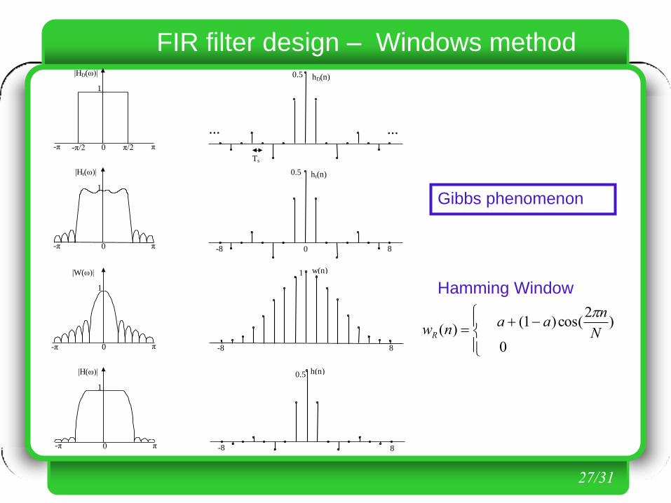
27/31
-π/2 π/2
1
-π π 0
|HD(ω)|
1
-π π 0
|H(ω)|
1
-π π 0
|Ht(ω)|
1
-π π 0
|W(ω)|
0.5
0.5
ht(n)
w(n) 1
0
0.5
-8
-8
-8
h(n)
8
8
8
Ts
... ...
hD(n)
FIR filter design – Windows method
0
)2
cos()1()( N
naa
nwR
Gibbs phenomenon
Hamming Window

28/31
FIR filter design – Optimal filters
Parks and McClellan method.
Distributes Approximation error from the discontinuity
all over the frequency band.

29/31
0 100 200 300 400 500
-80
-60
-40
-20
0
Frequency
Ma
gnitud
e
0 100 200 300 400 500-5
0
5
Frequency
Pha
se
0 5 10 15 20 25 30 35 40 45-0.2
0
0.2
0.4
Time
IR
0 100 200 300 400 500-90
-80
-70
-60
-50
-40
-30
-20
-10
0
Frequency
Ma
gni
tud
e
Windows: 61 Coefficients
Parks and McClellan method: 46
and equiripple
FIR filter design – Comparisons

30/31
FIR filters – Linear phase
Linear phase is strictly related with the symmetry of the Impulse Response
H h k e
h h e h e h e h e h e h e
e h e h e h e h h e h e h
j kT
k
j T j T j T j T j T j T
j T j T j T j T j T j T
( ) ( )
( ) ( ) ( ) ( ) ( ) ( ) ( )
( ) ( ) ( ) ( ) ( ) ( )
0
6
2 3 4 5 6
3 3 2 2
0 1 2 3 4 5 6
0 1 2 3 4 5
( )
( )( ) ( )( ) ( )( ) ( )
( )cos( ) ( )cos( ) ( )cos( ) ( )
6
0 1 2 3
2 0 3 2 1 2 2 2 3
3
3 3 3 2 2
3
e
e h e e h e e h e e h
e h T h T h T h
j T
j T j T j T j T j T j T j T
j T
( ) a ( ) b a
h n h N n( ) ( ) 1Condition
The phase is introduced by the term e-j3ωT and equals
θ(ω)=3ωΤ=ωΤ (7-1)/2

31/31
Linear phase - Same time delay
180o
If you shift in time one signal, then you have to shift the other signals the
same amount of time in order the final wave remains unchanged.
For faster signals the same time interval means larger phase difference.
Proportional to the frequency of the signals. -αω
5*180o
3*180o


![ECE-V-DIGITAL SIGNAL PROCESSING [10EC52] …vtusolution.in/.../digital-signal-processing-10ec52.pdfDigital vtusolution.in Signal Processing 10EC52 TEXT BOOK: 1. DIGITAL SIGNAL PROCESSING](https://static.documents.pub/doc/80x56/5afe42bb7f8b9a256b8ccd2e/ece-v-digital-signal-processing-10ec52-signal-processing-10ec52-text-book.jpg)
![Digital Audio Signal Processing DASPdspuser/dasp/material...2 Digital Audio Signal Processing Version 2016-2017 Lecture-5: Adaptive Beamforming 3 / 34 F 1 (ω) F 2 (ω) F M (ω) z[k]](https://static.documents.pub/doc/80x56/60097e450147c810167b0d60/digital-audio-signal-processing-dasp-dspuserdaspmaterial-2-digital-audio-signal.jpg)