Research, Development and Technology MoDOT RDT 05-007 Behavior and Fatigue Properties of Metalic Dampers for Seismic Retrofit of Highway Bridges April, 2005 RI 01-028 University of Missouri/Rolla
Transcript
Research, Development and Technology
MoDOT
RDT 05-007
Behavior and Fatigue Properties of Metalic Dampers for Seismic Retrofit of Highway Bridges
April, 2005
RI 01-028
University of Missouri/Rolla
Final Report
RDT 05-007
BEHAVIOR AND FATIGUE PROPERTIES OF METALLIC DAMPERS FOR SEISMIC RETROFIT OF HIGHWAY BRIDGES
MISSOURI DEPARTMENT OF TRANSPORTATION RESEARCH, DEVELOPMENT AND TECHNOLOGY
By: Genda Chen and Stephen Alan Eads
Acknowledgments: U.S. Department of Transportation through University Transportation Center at the University of Missouri-Rolla
JEFFERSON CITY, MISSOURI DATE SUBMITTED: April 15, 2005
The opinions, findings, and conclusions expressed in this publication are those of the principal investigators and the Missouri Department of Transportation; Research, Development and Technology. They are not necessarily those of the U.S. Department of Transportation, Federal Highway Administration. This report does not constitute a standard or regulation.
ii
TECHNICAL REPORT DOCUMENTATION PAGE
1. Report No. 2. Government Accession No.
3. Recipient's Catalog No.
RDT 05-007 4. Title and Subtitle 5. Report Date
April 15, 2005 6. Performing Organization Code
Behavior and Fatigue Properties of Metallic Dampers for Seismic Retrofit of Highway Bridges University of Missouri – Rolla 7. Author(s) 8. Performing Organization Report No.Genda Chen and Stephen Allen Eads RDT 05-007/RI 01-028 9. Performing Organization Name and Address 10. Work Unit No.
11. Contract or Grant No.
Missouri Department of Transportation Research, Development and Technology P. O. Box 270-Jefferson City, MO 65102 12. Sponsoring Agency Name and Address 13. Type of Report and Period Covered
Final Report 14. Sponsoring Agency Code
Missouri Department of Transportation Research, Development and Technology P. O. Box 270-Jefferson City, MO 65102 MoDOT 15. Supplementary Notes The investigation was conducted in cooperation with the U. S. Department of Transportation through the University Transportation Center at the University of Missouri-Rolla. 16. Abstract The objective of this study is to develop an economical solution with metallic dampers for the seismic retrofit of highway bridges in low occurrence seismic zones, such as in the Central and Eastern United States. Select low carbon steel rods were first tested for their ductile behavior and material strength. Large-scale, tapered rods were then tested for their energy dissipation capability and fatigue strength under regular, irregular, and earthquake loads. A full-scale damper made of five tapered rods was designed next for the seismic retrofit of a three-span continuous steel-girder bridge in southeast Missouri; its system performance including joints and connection members was validated with laboratory tests. The damping ratio of tapered rods was shown independent of loading frequency and specimen size; it rapidly increased at small displacements and approached a value of 0.35~0.40 in the range of over 1.8". Even at a displacement of 2.4", the steel rods can survive over 100 cycles of loading with little degradation of their damping property. The full-scale, five-rod damper has been demonstrated to reveal a progressive failure mode that is desirable for earthquake applications. Hysteretic models of Type D rocker bearings were developed for possible consideration in the seismic retrofit design of seismically inadequate highway bridges. 17. Key Words 18. Distribution Statement Seismic retrofit, metallic damper, energy dissipation, fatigue strength, highway bridges, material properties
No restrictions. This document is available to the public through National Technical Information Center, Springfield, Virginia 22161
19. Security Classification (of this report)
20. Security Classification (of this page)
21. No. of Pages 22. Price
Unclassified Unclassified 94 Form DOT F 1700.7 (06/98)
iii
EXECUTIVE SUMMARY
The objective of this study was to develop an economical solution for the seismic retrofit of existing highway bridges in low occurrence seismic zones, such as in the Central and Eastern United States. To achieve this objective, metallic dampers were introduced to protect bridge structures from being damaged by dissipating a significant portion of the seismic energy that is traditionally stored in structural members in the form of strain energy. The scopes of this study included a) select and test small-scale, low carbon steel rods for their ductile behavior and material strength; b) test large-scale, tapered rods for their energy dissipation capability and fatigue strength under regular, irregular, and earthquake loads; c) validate the system performance of a full-scale damper made of five tapered rods; d) address the implementation issues such as the performance of joints and connection members; and e) develop a hysteretic model of existing rocker bearings. In addition, the previously-proposed step-by-step procedure was examined and applied into the retrofit design of a three-span continuous steel-girder bridge in southeast Missouri.
Based on extensive numerical and experimental investigations in this report, the following conclusions can be drawn or recommendations can be made:
• Low carbon steels, Hot Rolled AISI/SAE1018, have a yielding stress of 32 ksi. These readily-available materials are recommended for the development of an economic yet effective solution for the seismic retrofit of highway bridges in low occurrence seismic regions.
• The effective stiffness of tapered steel rods decreases steadily as the applied displacement of harmonic loading increases. However, the damping ratio of the tapered rods, independent of loading frequency and specimen size, increases rapidly at small displacement and approaches to a value of 0.35~0.40 at displacement of over 1.8".
• At a high displacement of 2.4" or less, steel rods can survive over 100 cycles of loading without degrading their load-displacement hysteresis loops. They fracture at the mid-height of the cantilevered rods when welded to their base plate well. Under irregular loads, the fatigue strength of steel rods depends upon the sequence of loading; the commonly-used Miner’s rule could underestimate the strength of rods by 45%.
• For the Old St. Francis River Bridge, it is recommended that eight sets of five-rod dampers be installed on each of its two intermediate bents to make the three-span continuous steel-girder bridge seismic resistant. The validation test of one five-rod damper together with its supporting structural components, including a transverse beam and its shear connection with girders, proves that all five rods fail one by one near the highest stress location, resulting in a progressive failure mode that is desirable for earthquake applications. The performance of the damper and other structural components as a system is quite satisfactory.
• The seismic behavior of Type D expansion bearings can be simulated with a bi-linear model. The model parameters have been determined from the test results of 16 bearings retrieved from two decommissioned bridges. Test results from the earlier study also indicated that Type D bearings can accommodate an ultimate horizontal displacement of over 5" before they become unstable.
iv
ACKNOWLEDGMENTS
The authors would like to thank the Missouri Department of Transportation with Dr. Bryan A. Hartnagel as coordinator and the University Transportation Center at the University of Missouri-Rolla (UMR) for their financial support that made this project possible. Thanks are extended to Mr. Zhengshen Li for his contribution on the rocker bearing analysis portion of this study. The findings and opinions expressed in this report are those of the authors only; they may not necessarily represent those of the sponsors.
v
TABLE OF CONTENTS
Page LIST OF FIGURES ........................................................................................................ vii LIST OF TABLES ............................................................................................................ x
1. INTRODUCTION................................................................................................. 1 1.1. Background and Objectives ......................................................................... 1 1.2. Literature Review ......................................................................................... 1
1.2.1. Metals and Energy. ............................................................................... 1 1.2.2. Passive Energy Dissipation Systems.................................................... 3
1.3. REPORT ORGANIZATION....................................................................... 6 2. MATERIAL AND FATIGUE PROPERTIES ................................................... 7
2.1. Tensile Test .................................................................................................... 7 2.1.1. Member Selection.................................................................................. 7 2.1.2. Test Setup. ............................................................................................. 8 2.1.3. Results. ................................................................................................... 9
2.2. Fatigue Test ................................................................................................. 12 2.2.1. Member Selection................................................................................ 12 2.2.2. Test Setup. ........................................................................................... 13 2.2.3. Regular Loading.................................................................................. 16
2.2.3.1. Test Procedure. ............................................................................... 16 2.2.3.2. Results. ............................................................................................. 17
3. SEISMIC RETROFIT OF AN EXISTING HIGHWAY BRIDGE ............... 39 3.1. Background ................................................................................................. 39 3.2. Design Procedure ........................................................................................ 40
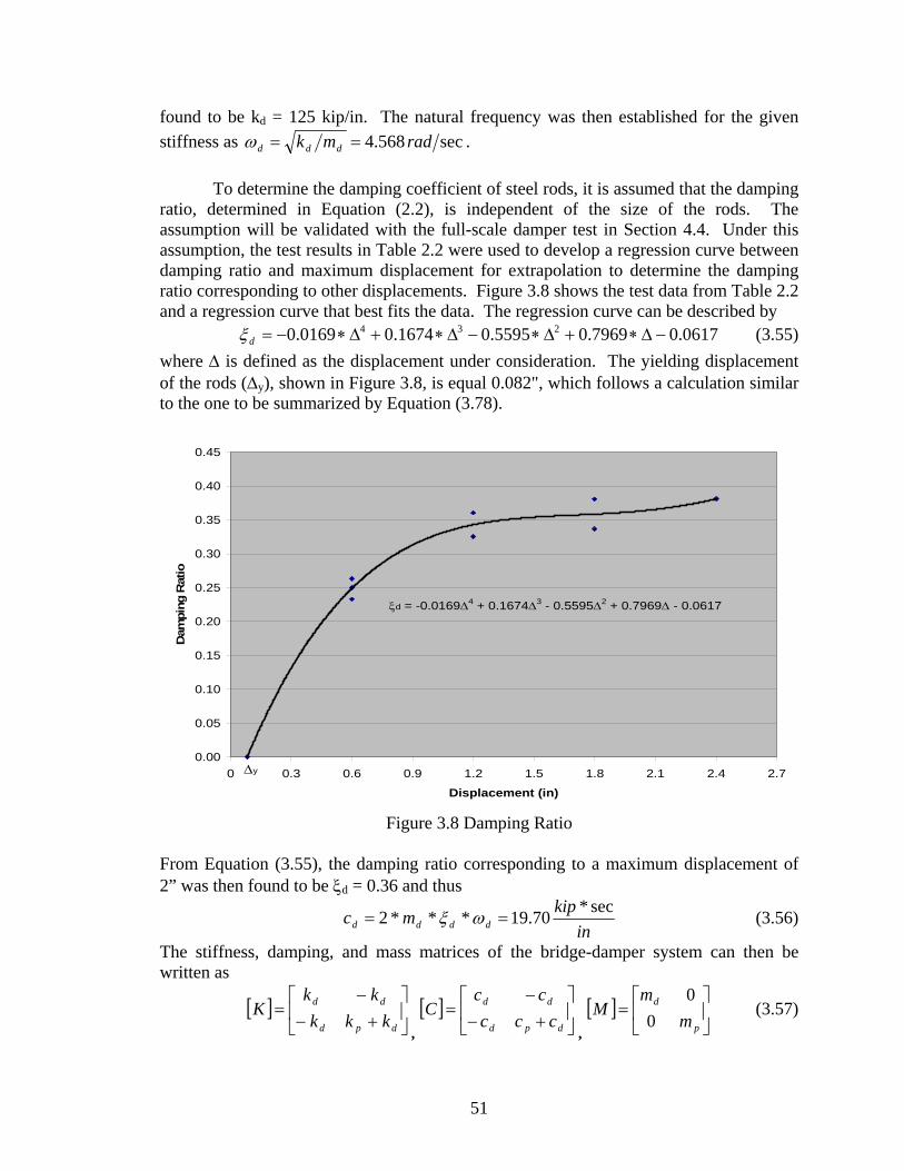
3.2.1. Loading. ............................................................................................... 40 3.2.1.1. Dead Load Per Column. ................................................................. 40 3.2.1.2. Total Mass........................................................................................ 41
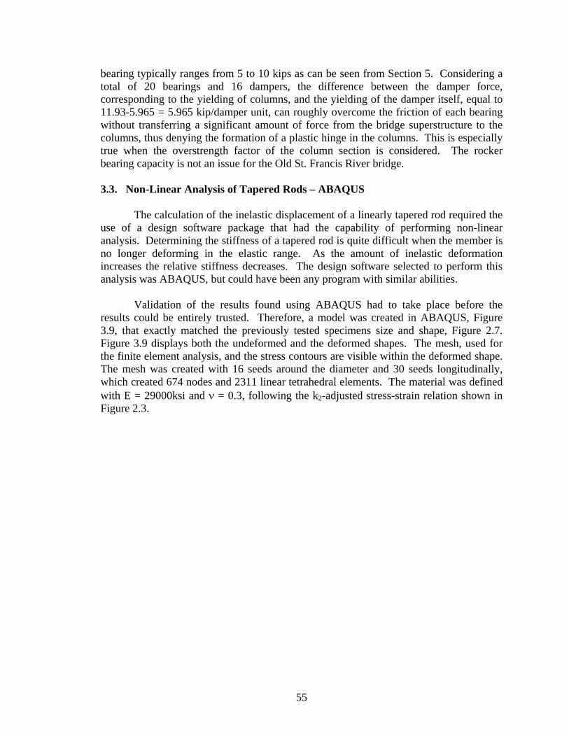
3.3. Non-Linear Analysis of Tapered Rods – ABAQUS ................................. 55 3.4. Design Summary and Cost ......................................................................... 57
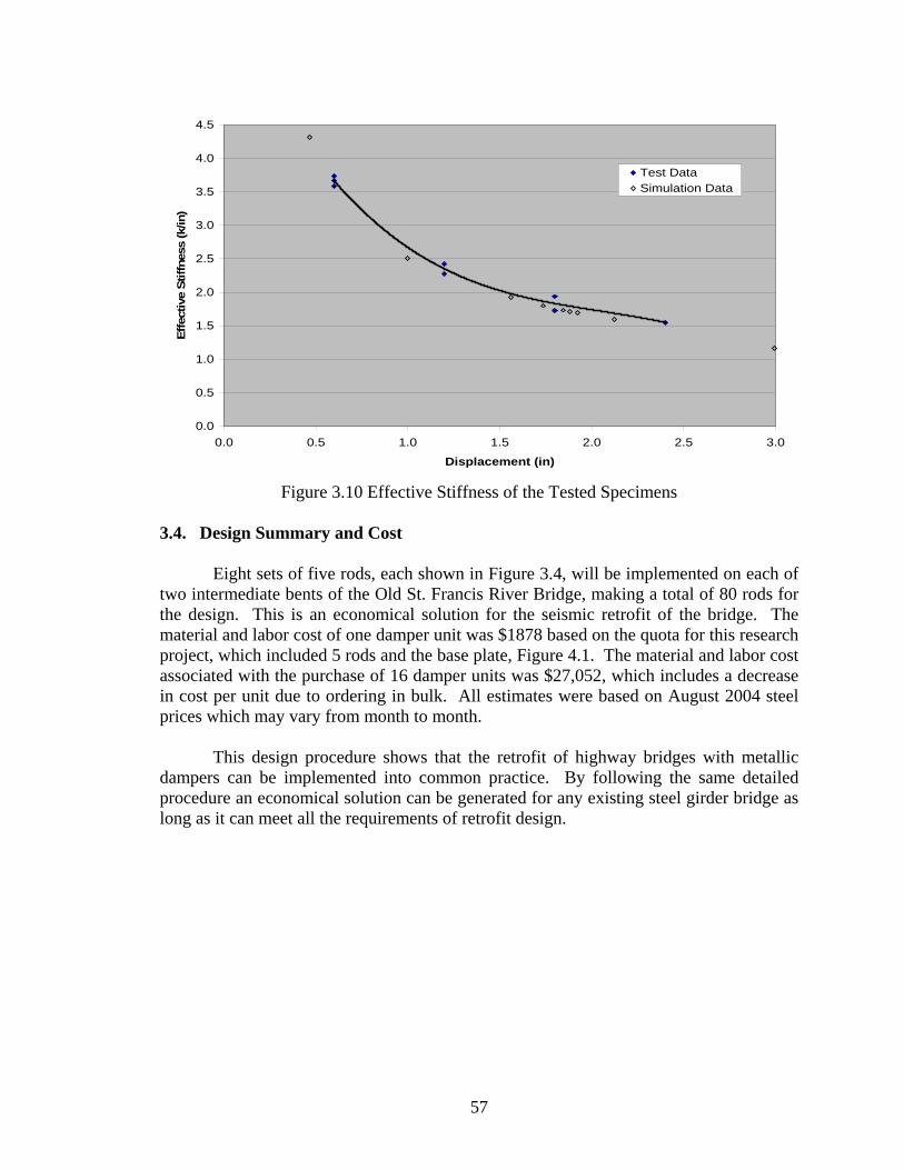
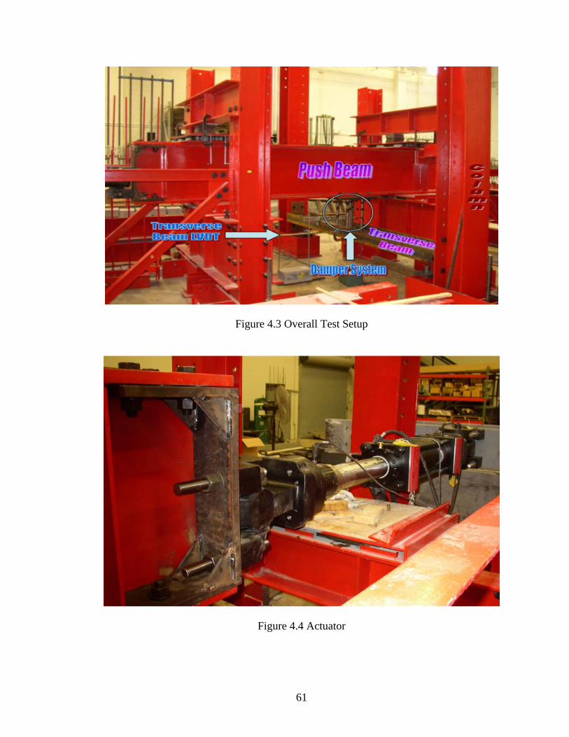
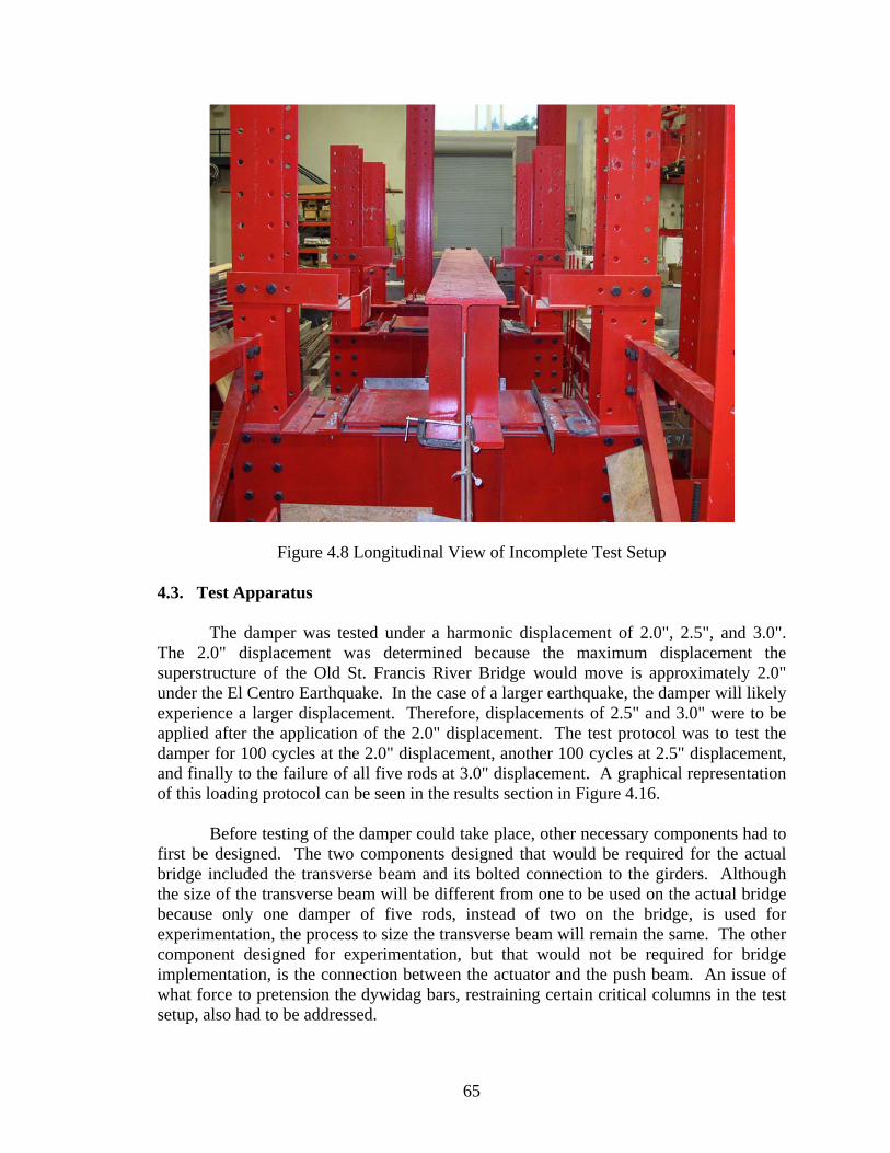
4. VALIDATION OF THE FULL SCALE METALLIC DAMPER ................. 58 4.1. Background ................................................................................................. 58 4.2. Test Setup .................................................................................................... 59 4.3. Test Apparatus ............................................................................................ 65
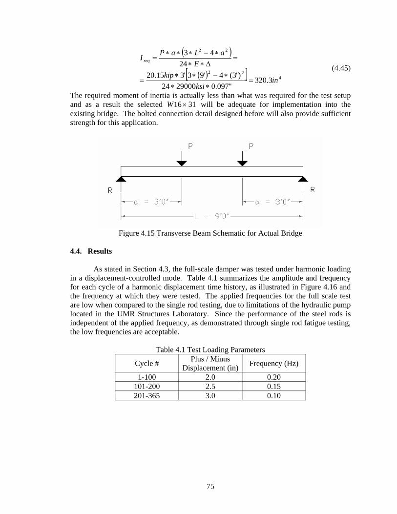
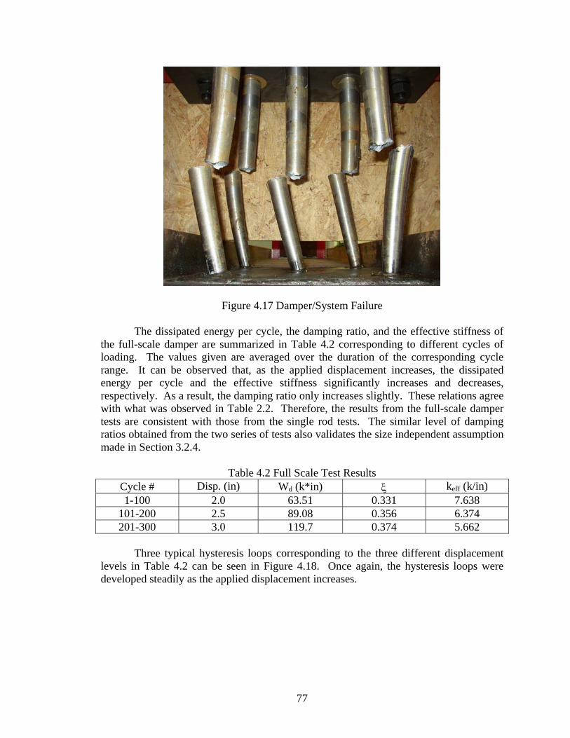
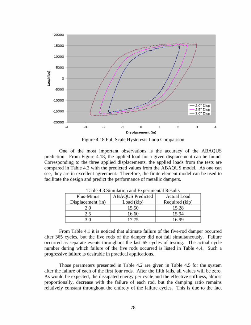
4.3.2. Bolted Connection for Transverse Beam. ......................................... 68 4.3.3. Actuator to Push Beam Connection. ................................................. 71 4.3.4. Column Restraint................................................................................ 73 4.3.5. Actual Design Bridge Apparatus. ...................................................... 74
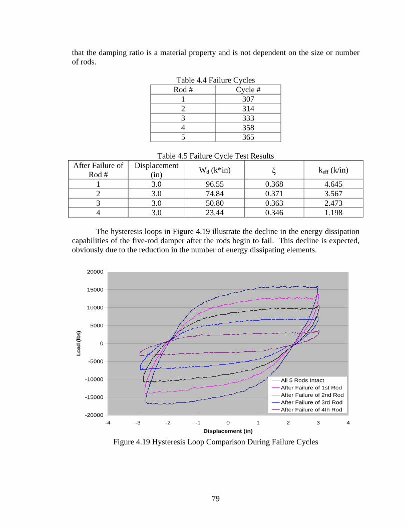
4.4. Results .......................................................................................................... 75 5. ANALYTICAL MODEL OF TYPE D BEARINGS........................................ 80
5.1. Background ................................................................................................. 80 5.2. Hysteretic Model of Longitudinal Behavior ............................................. 80
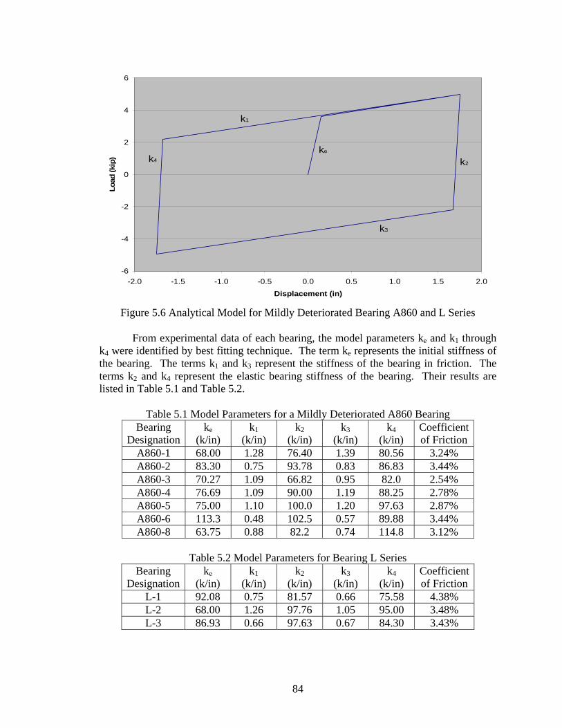
5.2.1. Mildly Deteriorated A860 and L Series Bearings. ........................... 82 5.2.2. Mildly Deteriorated A1005 Series Bearings. .................................... 85 5.2.3. Heavily Deteriorated A1005 Series Bearings. .................................. 87 5.2.4. Ultimate Behavior of Type D Bearings. ............................................ 89
LIST OF FIGURES Page Figure 1.1 Metallic Damper Geometries (Skinner et al. 1975)........................................... 4 Figure 1.2 ADAS Element Geometry (Whittaker et al. 1991) ........................................... 5 Figure 1.3 X-shaped Plate Damper (Soong and Dargush 1997)......................................... 5 Figure 2.1 Tensile Test Specimen....................................................................................... 8 Figure 2.2 MTS880 Testing Machine................................................................................. 9 Figure 2.3 Tensile Test Specimen #1................................................................................ 10 Figure 2.4 Tensile Test Specimen #2................................................................................ 11 Figure 2.5 Tensile Test Specimen #3................................................................................ 11 Figure 2.6 Tensile Test Comparison................................................................................. 12 Figure 2.7 Metallic Damper.............................................................................................. 13 Figure 2.8 Strain Gauge Locations ................................................................................... 14 Figure 2.9 Test Setup and Instrumentation ....................................................................... 14 Figure 2.10 Data Acquisition Unit.................................................................................... 15 Figure 2.11 MTS 407 Input Control Screen ..................................................................... 16 Figure 2.12 Typical Hysteresis Loop................................................................................ 17 Figure 2.13 Hysteresis Loop Comparison ........................................................................ 19 Figure 2.14 Failure Modes................................................................................................ 20 Figure 2.15 Maximum Strain Distribution for 0.6" Displacement ................................... 21 Figure 2.16 Strain Movement for Given Location............................................................ 22 Figure 2.17 Dissipated Energy Comparison ..................................................................... 23 Figure 2.18 Damping Ratio Comparison .......................................................................... 23 Figure 2.19 Effective Stiffness Comparison..................................................................... 24 Figure 2.20 Reduced Amplitude Displacement Time History of El Centro Earthquake.. 25 Figure 2.21 Reduced Amplitude Displacement Time History of Northridge Earthquake 25 Figure 2.22 Displacement History Corresponding to El Centro Earthquake.................... 29 Figure 2.23 Displacement History Corresponding to Northridge Earthquake ................. 29 Figure 2.24 Damping Ratio Corresponding to El Centro Loading................................... 30 Figure 2.25 Effective Stiffness Corresponding to El Centro Loading.............................. 31 Figure 2.26 Damping Ratio Corresponding to Northridge Loading................................. 31 Figure 2.27 Effective Stiffness Corresponding to Northridge Loading............................ 32 Figure 2.28 Validation of α and β .................................................................................... 33 Figure 2.29 Recorded Displacement Time History Corresponding to the 1940 El Centro
Earthquake ................................................................................................................ 34 Figure 2.30 Recorded Displacement Time History Corresponding to the 1994 Northridge
Earthquake ................................................................................................................ 35 Figure 2.31 Hysteresis Loops under Reduced El Centro Earthquake (First Cycle) ......... 36 Figure 2.32 Hysteresis Loops under Reduced El Centro Earthquake (Just Before Failure
Cycle)........................................................................................................................ 36 Figure 2.33 Hysteresis Loops under Reduced Northridge Earthquake (First Cycle) ....... 37 Figure 2.34 Hysteresis Loops under Reduced Northridge Earthquake (Just Before Failure
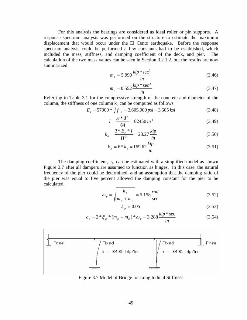
Cycle)........................................................................................................................ 37 Figure 3.1 General Elevation and Retrofit Scheme .......................................................... 39 Figure 3.2 Installation of Metallic Dampers ..................................................................... 39
viii
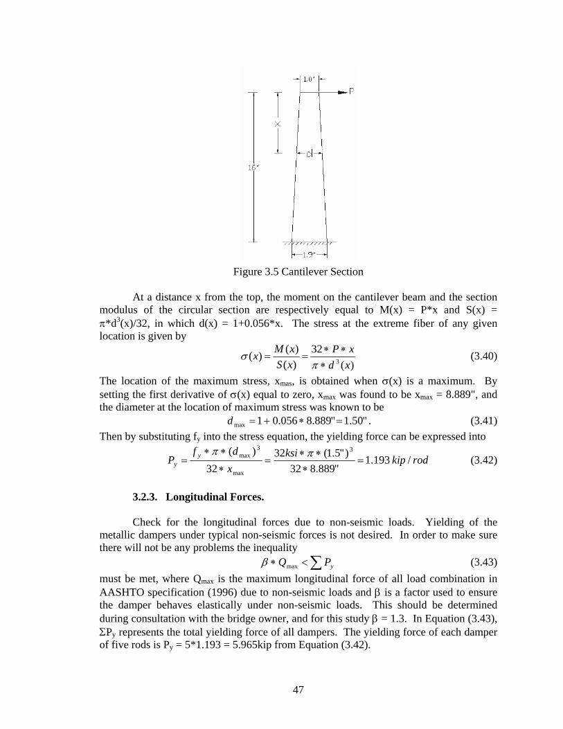
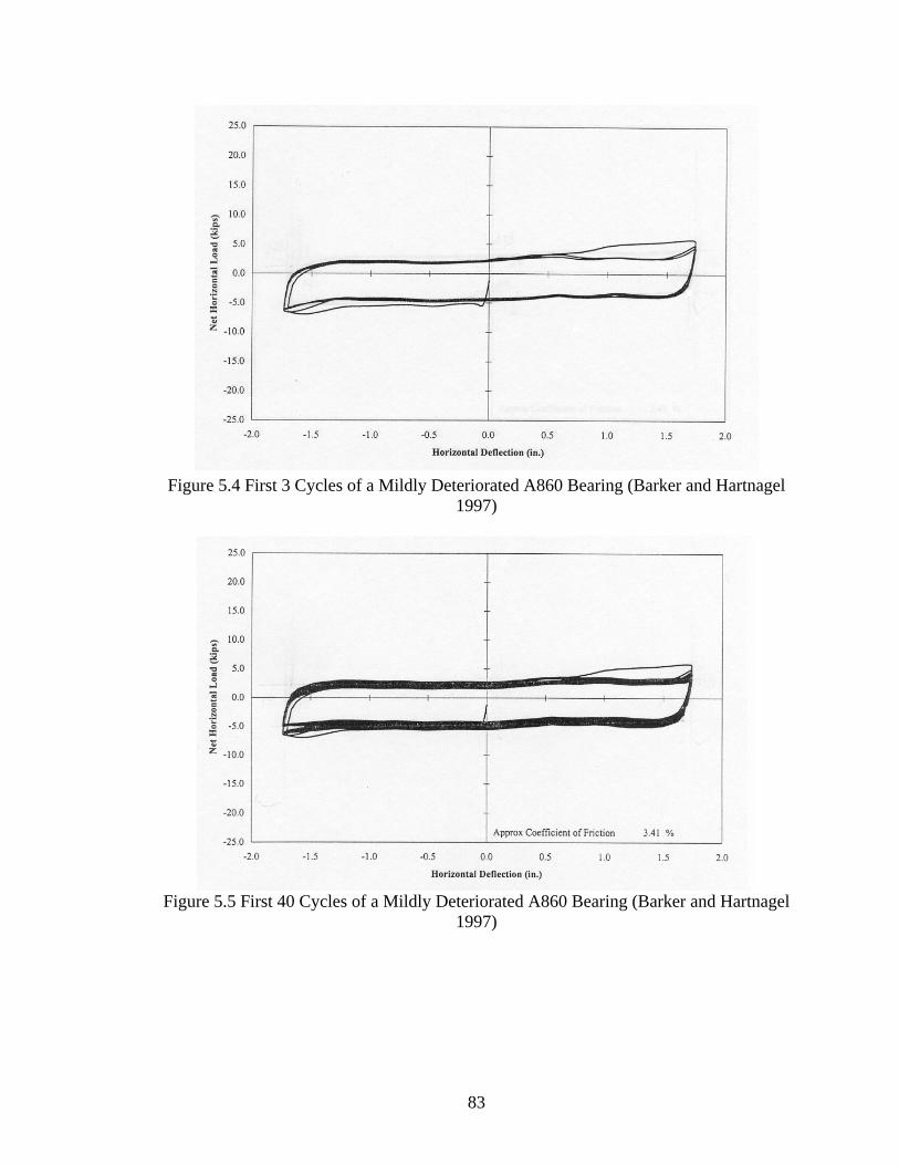
Figure 3.3 Column Cross Section ..................................................................................... 43 Figure 3.4 Selected Member for Retrofit Design.............................................................. 46 Figure 3.5 Cantilever Section ........................................................................................... 47 Figure 3.6 Two-Degree-of-Freedom Model of Bridge and Damper System.................... 48 Figure 3.7 Model of Bridge for Longitudinal Stiffness .................................................... 49 Figure 3.8 Damping Ratio................................................................................................. 51 Figure 3.9 Finite Element Model of One Steel Rod ......................................................... 56 Figure 3.10 Effective Stiffness of the Tested Specimens ................................................. 57 Figure 4.1 Five Rod Specimen.......................................................................................... 59 Figure 4.2 Test Setup Schematic ...................................................................................... 60 Figure 4.3 Overall Test Setup ........................................................................................... 61 Figure 4.4 Actuator ........................................................................................................... 61 Figure 4.5 Ball Joint Connections..................................................................................... 63 Figure 4.6 Ball Joint Close Up.......................................................................................... 63 Figure 4.7 Test Components Interaction........................................................................... 64 Figure 4.8 Longitudinal View of Incomplete Test Setup ................................................. 65 Figure 4.9 Simply Supported Beam.................................................................................. 67 Figure 4.10 Angle Connector Schematic .......................................................................... 69 Figure 4.11 Actual Angle Connector ................................................................................ 69 Figure 4.12 Connection Schematic ................................................................................... 72 Figure 4.13 Actual Connection ......................................................................................... 72 Figure 4.14 Force Relationship......................................................................................... 74 Figure 4.15 Transverse Beam Schematic for Actual Bridge ............................................ 75 Figure 4.16 Full Scale Test Load History......................................................................... 76 Figure 4.17 Damper/System Failure ................................................................................. 77 Figure 4.18 Full Scale Hysteresis Loop Comparison ....................................................... 78 Figure 4.19 Hysteresis Loop Comparison During Failure Cycles.................................... 79 Figure 5.1 Bearing A1005 (Barker and Hartnagel 1997) ................................................. 81 Figure 5.2 Bearing A860 (Barker and Hartnagel 1997) ................................................... 81 Figure 5.3 Bearing A860 (Barker and Hartnagel 1997) ................................................... 82 Figure 5.4 First 3 Cycles of a Mildly Deteriorated A860 Bearing (Barker and Hartnagel
1997) ........................................................................................................................ 83 Figure 5.5 First 40 Cycles of a Mildly Deteriorated A860 Bearing (Barker and Hartnagel
1997) ......................................................................................................................... 83 Figure 5.6 Analytical Model for Mildly Deteriorated Bearing A860 and L Series.......... 84 Figure 5.7 First 3 Cycles of a Mildly Deteriorated A1005 Bearing (Barker and Hartnagel
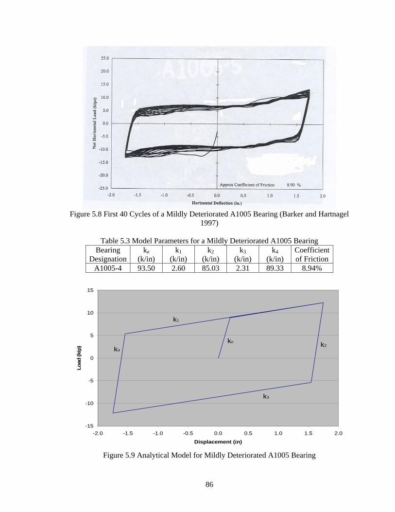
1997) ......................................................................................................................... 85 Figure 5.8 First 40 Cycles of a Mildly Deteriorated A1005 Bearing (Barker and Hartnagel
1997) ......................................................................................................................... 86 Figure 5.9 Analytical Model for Mildly Deteriorated A1005 Bearing............................. 86 Figure 5.10 First 3 Cycles of a Heavily Deteriorated A1005 Bearing (Barker and
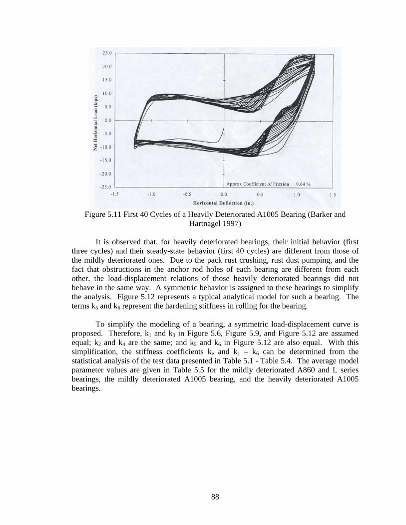
Hartnagel 1997) ........................................................................................................ 87 Figure 5.11 First 40 Cycles of a Heavily Deteriorated A1005 Bearing (Barker and
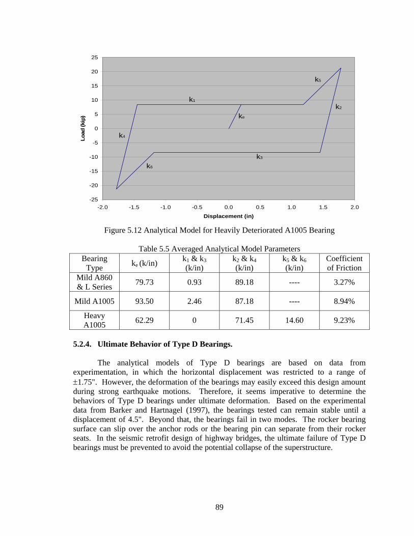
Hartnagel 1997) ....................................................................................................... 88 Figure 5.12 Analytical Model for Heavily Deteriorated A1005 Bearing ......................... 89
ix
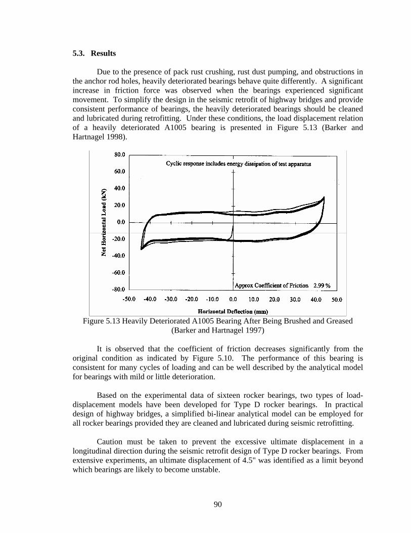
Figure 5.13 Heavily Deteriorated A1005 Bearing After Being Brushed and Greased (Barker and Hartnagel 1997) .................................................................................... 90
x
LIST OF TABLES Page Table 1.1 Fatigue Life at Various Strain Amplitudes and Frequencies.............................. 2 Table 1.2 Effect of Different Cycle Load Histories............................................................ 3 Table 1.3 Applied Earthquakes to Failure .......................................................................... 3 Table 2.1 Test Loading Parameters .................................................................................. 18 Table 2.2 Test Result Comparison.................................................................................... 18 Table 2.3 Number of Cycles (n) Representing One Earthquake ...................................... 26 Table 2.4 Fatigue Life (N) for Corresponding Displacement........................................... 27 Table 2.5 Total Applied Cycles ........................................................................................ 27 Table 2.6 Total Cycles at 10% for each Earthquake......................................................... 28 Table 2.7 Cycle Count Comparison.................................................................................. 38 Table 3.1 Material and Geometric Properties ................................................................... 43 Table 4.1 Test Loading Parameters .................................................................................. 75 Table 4.2 Full Scale Test Results...................................................................................... 77 Table 4.3 Simulation and Experimental Results............................................................... 78 Table 4.4 Failure Cycles ................................................................................................... 79 Table 4.5 Failure Cycle Test Results ................................................................................ 79 Table 5.1 Model Parameters for a Mildly Deteriorated A860 Bearing ............................ 84 Table 5.2 Model Parameters for Bearing L Series............................................................ 84 Table 5.3 Model Parameters for a Mildly Deteriorated A1005 Bearing .......................... 86 Table 5.4 Model Parameters for a Heavily Deteriorated A1005 Bearing......................... 87 Table 5.5 Averaged Analytical Model Parameters ........................................................... 89
1
1. INTRODUCTION 1.1. Background and Objectives
The first version of the seismic design criteria was available in 1975 from the American Association of State Highway and Transportation Officials (AASHTO). In 1981 AASHTO approved the Seismic Design Guidelines for Highway Bridges, which was published by the Federal Highway Administration. This was accepted as the standard specification throughout the United States for bridge design. Prior to these design codes little seismic evaluation was performed, particularly in the Eastern and Central United States, and as a result there are many existing bridges that are inadequately prepared for a seismic event. On the other hand, no strong earthquake has struck this area since 1811-1812 though small earthquakes occur on a regular basis. Therefore, it is imperative to develop an economical solution for the seismic retrofit of existing highway bridges in low occurrence seismic zones in the Central and Eastern United States.
Previous studies by Chen et al. (2001) indicated that metallic dampers consisting
of low carbon steel prismatic rods can be used to mitigate the seismic responses of bridge structures. As a continuation of the previous study, the purpose of this study is to address several issues related to the implementation of metallic dampers in steel-girder bridges with rocker bearings. Specifically, the objectives of this study are:
• to further improve the performance of dampers with tapered rods, • to establish design equations for the damping property of tapered metallic
dampers, • to validate the previously-proposed design procedure for bridge systems including
metallic dampers, • to study the effect of transverse beams, used to connect dampers from capbeam to
steel girders, on the damping properties of dampers, and • to develop a hysteresis model of the load carrying capacity of rocker bearings.
1.2. Literature Review
Low carbon steel rods and plates, or metallic dampers, have been studied over the past 25 years mainly for the dissipation of earthquake energy into buildings. Little has been studied for bridge structures. Some of the important developments in metallic dampers are summarized and discussed below. 1.2.1. Metals and Energy.
Tapered steel cantilevered rods have been fabricated with materials from other countries and tested as mechanical energy dissipaters through plastic deformation during flexure (Buckle and King 1980). Twenty dissipaters composed of Grade 43A black mild steel to BS 4360 steel were tested. Testing was completed under regular sinusoidal loading, irregular sinusoidal loading, and also with actual earthquake input. Regular loading implied that the strain magnitude was held constant during the entire test and the
2
opposite was true for the irregular testing. During the later stages of testing for the higher strain applications a small relative movement between the actual specimen and the base began. The gap grew as the plastic deformation became more significant. This forced the use of strain controlled loading instead of displacement controlled, to account for this movement and corresponding reduction in rigidity. Temperature rise in the specimens limited the number of cycles to be performed at a time, but the amount of rise was independent of the applied frequency.
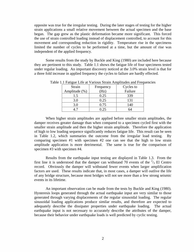
Some results from the study by Buckle and King (1980) are included here because
they are pertinent to this study. Table 1.1 shows the fatigue life of four specimens tested under regular loading. An important discovery noticed at the 3.0% strain level is that for a three fold increase in applied frequency the cycles to failure are hardly effected.
Table 1.1 Fatigue Life at Various Strain Amplitudes and Frequencies Strain
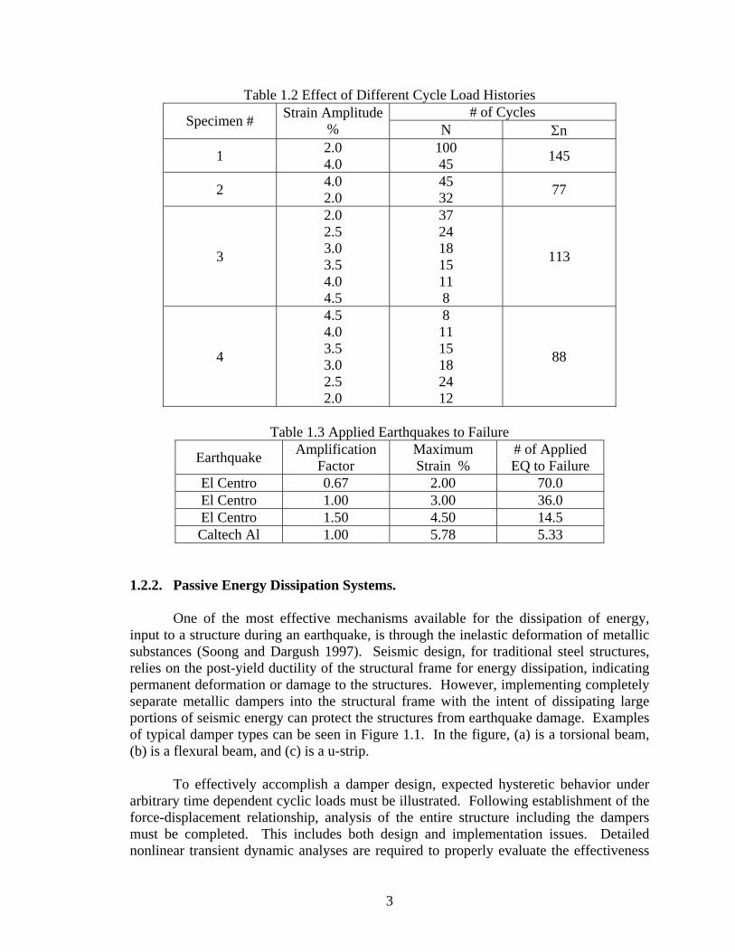
When higher strain amplitudes are applied before smaller strain amplitudes, the
damper receives greater damage than when compared to a specimen cycled first with the smaller strain amplitude and then the higher strain amplitude. Therefore the application of high to low loading sequence significantly reduces fatigue life. This result can be seen in Table 1.2, which summaries the outcome from the irregular load testing. By comparing specimen #1 with specimen #2 one can see that the high to low strain amplitude application is more detrimental. The same is true for the comparison of specimen #3 with specimen #4.
Results from the earthquake input testing are displayed in Table 1.3. From the
first line it is understood that the damper can withstand 70 events of the 2/3 El Centro record. Obviously the damper will withstand fewer events when larger amplification factors are used. These results indicate that, in most cases, a damper will outlive the life of any bridge structure, because most bridges will not see more than a few strong seismic events in its lifetime.
An important observation can be made from the tests by Buckle and King (1980).
Hysteresis loops generated through the actual earthquake input are very similar to those generated through varying displacements of the regular sinusoidal loading. The regular sinusoidal loading applications produce similar results, and therefore are expected to adequately describe the dissipater properties under earthquake loading. The actual earthquake input is not necessary to accurately describe the attributes of the damper, because their behavior under earthquake loads is well predicted by cyclic testing.
3
Table 1.2 Effect of Different Cycle Load Histories # of Cycles Specimen # Strain Amplitude
% N Σn
1 2.0 4.0
100 45 145
2 4.0 2.0
45 32 77
3
2.0 2.5 3.0 3.5 4.0 4.5
37 24 18 15 11 8
113
4
4.5 4.0 3.5 3.0 2.5 2.0
8 11 15 18 24 12
88
Table 1.3 Applied Earthquakes to Failure
Earthquake Amplification Factor
Maximum Strain %
# of Applied EQ to Failure
El Centro 0.67 2.00 70.0 El Centro 1.00 3.00 36.0 El Centro 1.50 4.50 14.5 Caltech Al 1.00 5.78 5.33
1.2.2. Passive Energy Dissipation Systems.
One of the most effective mechanisms available for the dissipation of energy, input to a structure during an earthquake, is through the inelastic deformation of metallic substances (Soong and Dargush 1997). Seismic design, for traditional steel structures, relies on the post-yield ductility of the structural frame for energy dissipation, indicating permanent deformation or damage to the structures. However, implementing completely separate metallic dampers into the structural frame with the intent of dissipating large portions of seismic energy can protect the structures from earthquake damage. Examples of typical damper types can be seen in Figure 1.1. In the figure, (a) is a torsional beam, (b) is a flexural beam, and (c) is a u-strip.
To effectively accomplish a damper design, expected hysteretic behavior under
arbitrary time dependent cyclic loads must be illustrated. Following establishment of the force-displacement relationship, analysis of the entire structure including the dampers must be completed. This includes both design and implementation issues. Detailed nonlinear transient dynamic analyses are required to properly evaluate the effectiveness
4
of any real structure employing metallic dampers for enhanced seismic protection. The finite element method provides the most suitable framework for a multi-degree-of- freedom analysis of an overall structure (Soong and Dargush 1997).
Figure 1.1 Metallic Damper Geometries (Skinner et al. 1975)
A number of researchers and practitioners have continued to implement these devices in full scale structures after gaining confidence in metallic damper performance based primarily on experimental evidence. New Zealand has the first recorded implementation of energy dampers into a structural system, but more recently other countries have joined the list. Countries such as Mexico, Japan, Italy, and the United States also include energy dampers necessary for the design of structural frames.
The discussions of various related experiments and actual existing structural
implementations are included in Soong and Dargush (1997). Reports of four such experiments include those presented by Kelly et al. (1972), Skinner et al. (1975), Bergman and Goel (1987), and Whittaker et al. (1991).
Included within Whittaker et al. (1991) was a comprehensive discussion of an
experimental program that was performed at the University of California at Berkeley. This particular experiment focused on the evaluation of an X-shaped plate damper known as Added Damping And Stiffness (ADAS) elements. Dimensional characteristics of the ADAS element are presented in Figure 1.2, and an actual ADAS can be seen in Figure 1.3.
5
Figure 1.2 ADAS Element Geometry (Whittaker et al. 1991)
Figure 1.3 X-shaped Plate Damper (Soong and Dargush 1997)
Many existing structures that include metallic energy dissipaters were discussed. The Rangitikei Bridge in New Zealand made use of a torsion beam steel damper for the piers. The thirteen story Izazaga #38-40 Building constructed in the late 1970s near Mexico City underwent numerous seismic attacks. In 1990 250 ADAS elements were installed to permit continued building operation. Another Mexican application on the six-story Cardiology Hospital Building was also constructed in the late 1970s. In 1990 a total of 90 ADAS dampers were connected to the building via 18 external buttresses. The two-story Wells Fargo Bank building in San Francisco was constructed in 1967 and was damaged by the 1989 Loma Prieta earthquake. The seismic upgrade included chevron braces and seven ADAS damping elements, each with a yielding force of 150 kips.
6
1.3. REPORT ORGANIZATION
A detailed discussion of the design, analysis, and experimentation of metallic dampers with tapered rods is included in this report. The developments of material properties through tensile testing and of the tapered rod’s characteristics through fatigue testing are presented in Section 2. The seismic retrofit design procedure with metallic dampers is then outlined and applied into an existing bridge in Section 3. System performance validation of the full scale dampers, designed in Section 3, and their supporting structural components is presented in Section 4. An analytical model representing the behavior of the various categories of Type D expansion rocker bearings is presented in Section 5. The major conclusions and recommendations from this study are summarized in Section 6.
7
2. MATERIAL AND FATIGUE PROPERTIES 2.1. Tensile Test
As stated in Section 1, the ultimate goal of this study is to develop an economical solution for the design and retrofit of continuous steel girder bridges in low occurrence seismic zones. To accomplish this, the main part of the research project is to test several dampers to ensure their energy dissipation capability and fatigue resistance. For this application, low carbon steels are ideal materials. Location of such a material was not an easy task, but an appropriate steel material and a fabricator to make the dampers were identified. The material used was Hot Rolled (HR) AISI/SAE 1018 and was supplied by Ryerson Tull, St. Louis. HR 1018 has a relatively low carbon content (0.15%-0.20%) which makes this material much more ductile than most steels available in the market. High ductility is required for the dampers to be effective in dissipating the destructive power of an earthquake. The low carbon content also implies that the material will have a smaller yielding stress than materials having higher carbon contents. Having a small yield stress will ensure that the material will act inelastically during excitation from an earthquake, which is exactly what is needed if the dampers are to be effective in dissipating energy. 2.1.1. Member Selection.
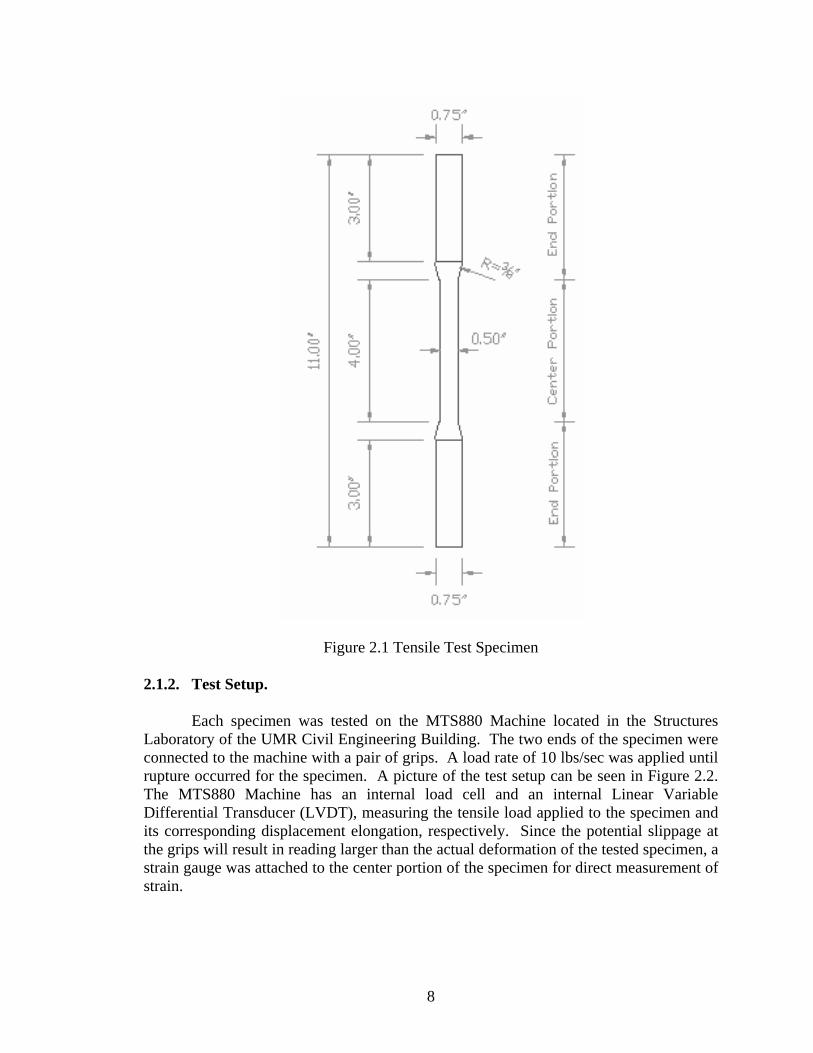
To guarantee the material properties of HR 1018 would be acceptable, the need to test a small quantity of the material was evident. The size of the three round specimens that were tested in tension ranged from ½" (center portion) to ¾" and they were eleven inches in height. It is schematically shown in Figure 2.1.
8
Figure 2.1 Tensile Test Specimen 2.1.2. Test Setup.
Each specimen was tested on the MTS880 Machine located in the Structures Laboratory of the UMR Civil Engineering Building. The two ends of the specimen were connected to the machine with a pair of grips. A load rate of 10 lbs/sec was applied until rupture occurred for the specimen. A picture of the test setup can be seen in Figure 2.2. The MTS880 Machine has an internal load cell and an internal Linear Variable Differential Transducer (LVDT), measuring the tensile load applied to the specimen and its corresponding displacement elongation, respectively. Since the potential slippage at the grips will result in reading larger than the actual deformation of the tested specimen, a strain gauge was attached to the center portion of the specimen for direct measurement of strain.
9
Figure 2.2 MTS880 Testing Machine 2.1.3. Results.
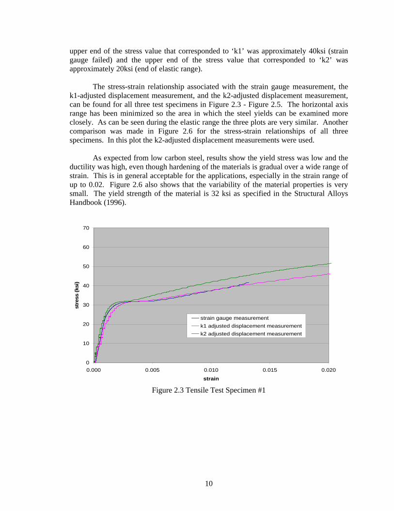
The MTS880 Machine gave a digital readout of load and displacement every two seconds. The load could then be transformed into a stress by dividing it by the cross sectional area of the center portion of the specimen, and the displacement measurement could then be transformed into a strain by dividing the measured elongation between the two grips with the length of the center portion. The strain in the specimen was also acquired until the strain gauge fails at its design value, which is approximately ten times the yield strain. The stress determined can then be plotted against the strain as respectively shown in Figure 2.3, Figure 2.4, and Figure 2.5 for each of the three tested specimens.
The readout from the strain gauge, during its short but effective lifespan, was
more accurate than the strain value derived by dividing the displacement by the length of the center portion (derived strain). Because of this fact and the fact that the strain gauge failed before the test was complete, the need to use the derived strain but correct it in a way to make it as similar as possible to the strain gauge readout for the applicable range was evident. Each test was altered by using a ‘k’ factor. This ‘k’ factor was found by calculating the slope of a plot between the derived strains and the strains from the gauge. In Figure 2.3 - Figure 2.5, two ‘k’ factors are introduced. The difference between the two is the range for which each slope was viewed. For each test ‘k1’ was found by calculating the previously mentioned slope in the range up until the strain gauge failed, while ‘k2’ was found as the specimen was still in the elastic range. For comparison, the
10
upper end of the stress value that corresponded to ‘k1’ was approximately 40ksi (strain gauge failed) and the upper end of the stress value that corresponded to ‘k2’ was approximately 20ksi (end of elastic range).
The stress-strain relationship associated with the strain gauge measurement, the
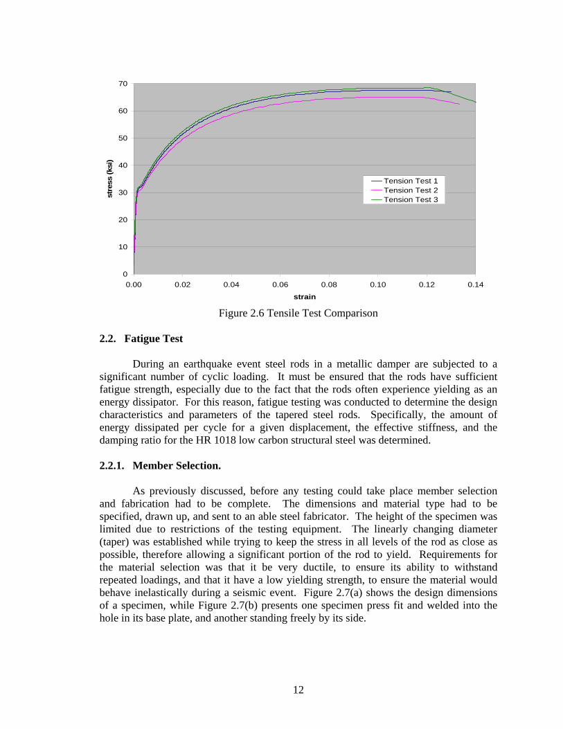
k1-adjusted displacement measurement, and the k2-adjusted displacement measurement, can be found for all three test specimens in Figure 2.3 - Figure 2.5. The horizontal axis range has been minimized so the area in which the steel yields can be examined more closely. As can be seen during the elastic range the three plots are very similar. Another comparison was made in Figure 2.6 for the stress-strain relationships of all three specimens. In this plot the k2-adjusted displacement measurements were used.
As expected from low carbon steel, results show the yield stress was low and the
ductility was high, even though hardening of the materials is gradual over a wide range of strain. This is in general acceptable for the applications, especially in the strain range of up to 0.02. Figure 2.6 also shows that the variability of the material properties is very small. The yield strength of the material is 32 ksi as specified in the Structural Alloys Handbook (1996).
During an earthquake event steel rods in a metallic damper are subjected to a significant number of cyclic loading. It must be ensured that the rods have sufficient fatigue strength, especially due to the fact that the rods often experience yielding as an energy dissipator. For this reason, fatigue testing was conducted to determine the design characteristics and parameters of the tapered steel rods. Specifically, the amount of energy dissipated per cycle for a given displacement, the effective stiffness, and the damping ratio for the HR 1018 low carbon structural steel was determined. 2.2.1. Member Selection.
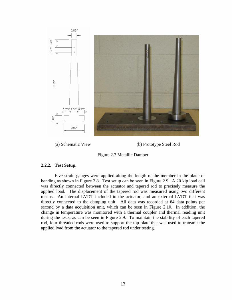
As previously discussed, before any testing could take place member selection and fabrication had to be complete. The dimensions and material type had to be specified, drawn up, and sent to an able steel fabricator. The height of the specimen was limited due to restrictions of the testing equipment. The linearly changing diameter (taper) was established while trying to keep the stress in all levels of the rod as close as possible, therefore allowing a significant portion of the rod to yield. Requirements for the material selection was that it be very ductile, to ensure its ability to withstand repeated loadings, and that it have a low yielding strength, to ensure the material would behave inelastically during a seismic event. Figure 2.7(a) shows the design dimensions of a specimen, while Figure 2.7(b) presents one specimen press fit and welded into the hole in its base plate, and another standing freely by its side.
13
(a) Schematic View (b) Prototype Steel Rod
Figure 2.7 Metallic Damper 2.2.2. Test Setup.
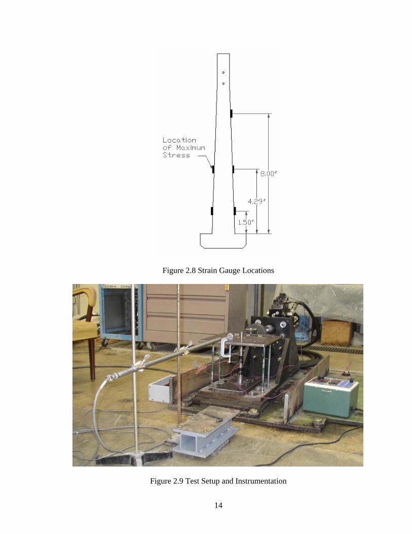
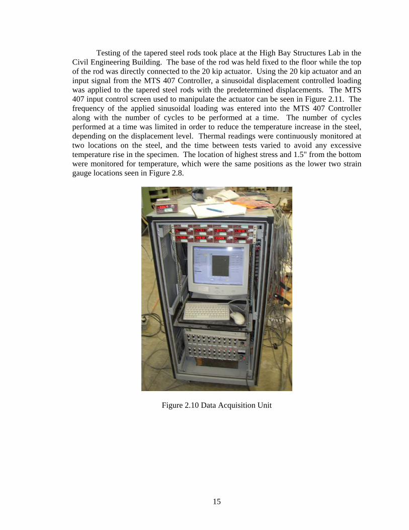
Five strain gauges were applied along the length of the member in the plane of bending as shown in Figure 2.8. Test setup can be seen in Figure 2.9. A 20 kip load cell was directly connected between the actuator and tapered rod to precisely measure the applied load. The displacement of the tapered rod was measured using two different means. An internal LVDT included in the actuator, and an external LVDT that was directly connected to the damping unit. All data was recorded at 64 data points per second by a data acquisition unit, which can be seen in Figure 2.10. In addition, the change in temperature was monitored with a thermal coupler and thermal reading unit during the tests, as can be seen in Figure 2.9. To maintain the stability of each tapered rod, four threaded rods were used to support the top plate that was used to transmit the applied load from the actuator to the tapered rod under testing.
14
Figure 2.8 Strain Gauge Locations
Figure 2.9 Test Setup and Instrumentation
15
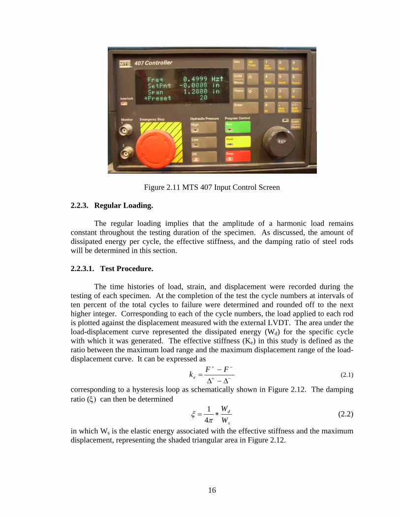
Testing of the tapered steel rods took place at the High Bay Structures Lab in the Civil Engineering Building. The base of the rod was held fixed to the floor while the top of the rod was directly connected to the 20 kip actuator. Using the 20 kip actuator and an input signal from the MTS 407 Controller, a sinusoidal displacement controlled loading was applied to the tapered steel rods with the predetermined displacements. The MTS 407 input control screen used to manipulate the actuator can be seen in Figure 2.11. The frequency of the applied sinusoidal loading was entered into the MTS 407 Controller along with the number of cycles to be performed at a time. The number of cycles performed at a time was limited in order to reduce the temperature increase in the steel, depending on the displacement level. Thermal readings were continuously monitored at two locations on the steel, and the time between tests varied to avoid any excessive temperature rise in the specimen. The location of highest stress and 1.5" from the bottom were monitored for temperature, which were the same positions as the lower two strain gauge locations seen in Figure 2.8.
Figure 2.10 Data Acquisition Unit
16
Figure 2.11 MTS 407 Input Control Screen 2.2.3. Regular Loading.
The regular loading implies that the amplitude of a harmonic load remains constant throughout the testing duration of the specimen. As discussed, the amount of dissipated energy per cycle, the effective stiffness, and the damping ratio of steel rods will be determined in this section. 2.2.3.1. Test Procedure.
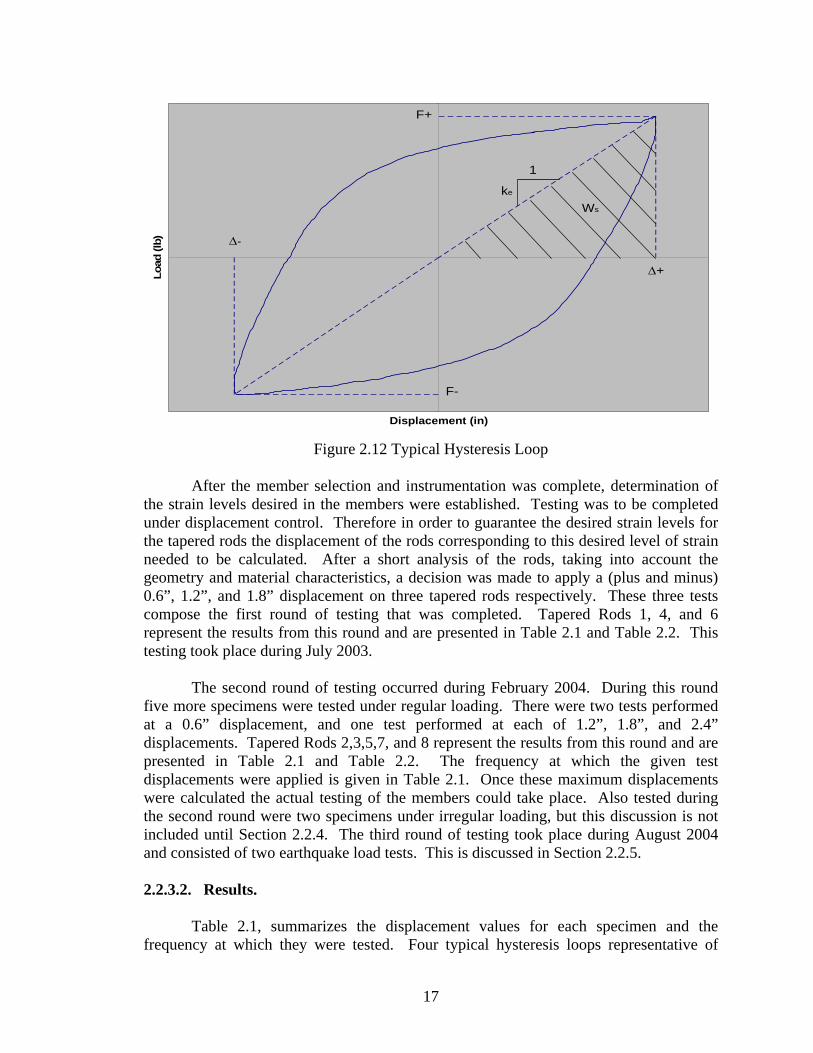
The time histories of load, strain, and displacement were recorded during the testing of each specimen. At the completion of the test the cycle numbers at intervals of ten percent of the total cycles to failure were determined and rounded off to the next higher integer. Corresponding to each of the cycle numbers, the load applied to each rod is plotted against the displacement measured with the external LVDT. The area under the load-displacement curve represented the dissipated energy (Wd) for the specific cycle with which it was generated. The effective stiffness (Ke) in this study is defined as the ratio between the maximum load range and the maximum displacement range of the load-displacement curve. It can be expressed as
−+
−+
∆−∆−
=FFke (2.1)
corresponding to a hysteresis loop as schematically shown in Figure 2.12. The damping ratio (ξ) can then be determined
s
d
WW
∗=π
ξ41 (2.2)
in which Ws is the elastic energy associated with the effective stiffness and the maximum displacement, representing the shaded triangular area in Figure 2.12.
17
Displacement (in)
Load
(lb) ∆-
∆+
F+
F-
ke
1
Ws
Figure 2.12 Typical Hysteresis Loop
After the member selection and instrumentation was complete, determination of
the strain levels desired in the members were established. Testing was to be completed under displacement control. Therefore in order to guarantee the desired strain levels for the tapered rods the displacement of the rods corresponding to this desired level of strain needed to be calculated. After a short analysis of the rods, taking into account the geometry and material characteristics, a decision was made to apply a (plus and minus) 0.6”, 1.2”, and 1.8” displacement on three tapered rods respectively. These three tests compose the first round of testing that was completed. Tapered Rods 1, 4, and 6 represent the results from this round and are presented in Table 2.1 and Table 2.2. This testing took place during July 2003.
The second round of testing occurred during February 2004. During this round
five more specimens were tested under regular loading. There were two tests performed at a 0.6” displacement, and one test performed at each of 1.2”, 1.8”, and 2.4” displacements. Tapered Rods 2,3,5,7, and 8 represent the results from this round and are presented in Table 2.1 and Table 2.2. The frequency at which the given test displacements were applied is given in Table 2.1. Once these maximum displacements were calculated the actual testing of the members could take place. Also tested during the second round were two specimens under irregular loading, but this discussion is not included until Section 2.2.4. The third round of testing took place during August 2004 and consisted of two earthquake load tests. This is discussed in Section 2.2.5. 2.2.3.2. Results.
Table 2.1, summarizes the displacement values for each specimen and the frequency at which they were tested. Four typical hysteresis loops representative of
18
different test displacements are presented in Figure 2.13. They came from Tapered Rods 2, 5, 7, and 8 and represent displacements of 0.6”, 1.2”, 1.8”, and 2.4”. Hysteresis loops such as these were used to generate the data presented in Table 2.2. It can be seen from this figure that the hysteresis loop was developed with an increasing enclosed area. Table 2.2 shows the number of cycles to failure, the average dissipated energy per cycle, the total dissipated energy, the average damping ratio, the effective stiffness, and the location of fracture. All averages included the values up to 90% of failure. Fracture location 1 represents failure along the base of the specimen, and fracture location 2 represents failure at the calculated location of highest stress.
Table 2.1 Test Loading Parameters
Tapered Rod # Plus / Minus Displacement (in) Frequency (Hz)
Several observations can be made from the results in Table 2.2, which are
grouped by test displacement in order to better show the similarities. For a given test displacement all results are very similar despite differences in the frequency at which they were tested. For example, three specimens (#1, #2, #3) were tested at a displacement of 0.6”, but they were loaded at a frequency of 0.25 Hz, 0.50 Hz, and 1.00 Hz respectively. Despite the difference in applied frequency their corresponding life to failure and their energy dissipating characteristics did not vary by any significant amount. The other displacement levels provided similar results. Therefore, the energy dissipater’s characteristics are independent of the applied frequency. A similar conclusion was drawn by Buckle and King (1980).
Another important observation is recognizing the decrease in effective stiffness as
the test displacements increase. The dramatic fall in post yield stiffness is an attractive feature of the dissipator since it implies that large plastic deformations, which are necessary for significant energy dissipation, may occur with only negligible increase in force (Buckle and King 1980).
Table 2.2 also indicates that, as the test displacement increases, the number of
cycles to failure and the average effective stiffness decreases significantly. As a result, even though the average dissipated energy per cycle increases, the total dissipated energy of every specimen is quite similar, implying the similar energy dissipation capability.
Theoretically the fracture location should be 4.286” up from the base of the
tapered rods because this location corresponds to the highest stress. Indeed, three of the eight specimens failed at this location as shown in Figure 2.14(a). Out of the five specimens that failed at the base, Figure 2.14(b), four had visible cracks in the weld
20
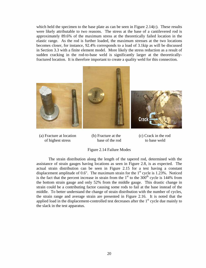
which held the specimen to the base plate as can be seen in Figure 2.14(c). These results were likely attributable to two reasons. The stress at the base of a cantilevered rod is approximately 89.6% of the maximum stress at the theoretically failed location in the elastic range. As the rod is further loaded, the maximum stresses at the two locations becomes closer, for instance, 92.4% corresponds to a load of 3.1kip as will be discussed in Section 3.3 with a finite element model. More likely the stress reduction as a result of sudden cracking in the rod-to-base weld is significantly larger at the theoretically-fractured location. It is therefore important to create a quality weld for this connection.
(a) Fracture at location (b) Fracture at the (c) Crack in the rod of highest stress base of the rod to base weld
Figure 2.14 Failure Modes
The strain distribution along the length of the tapered rod, determined with the assistance of strain gauges having locations as seen in Figure 2.8, is as expected. The actual strain distribution can be seen in Figure 2.15 for a test having a constant displacement amplitude of 0.6". The maximum strain for the 1st cycle is 1.23%. Noticed is the fact that the percent increase in strain from the 1st to the 300th cycle is 144% from the bottom strain gauge and only 52% from the middle gauge. This drastic change in strain could be a contributing factor causing some rods to fail at the base instead of the middle. To better understand the change of strain distribution with the number of cycles, the strain range and average strain are presented in Figure 2.16. It is noted that the applied load in the displacement-controlled test decreases after the 1st cycle due mainly to the slack in the test apparatus.
21
Figure 2.15 Maximum Strain Distribution for 0.6" Displacement
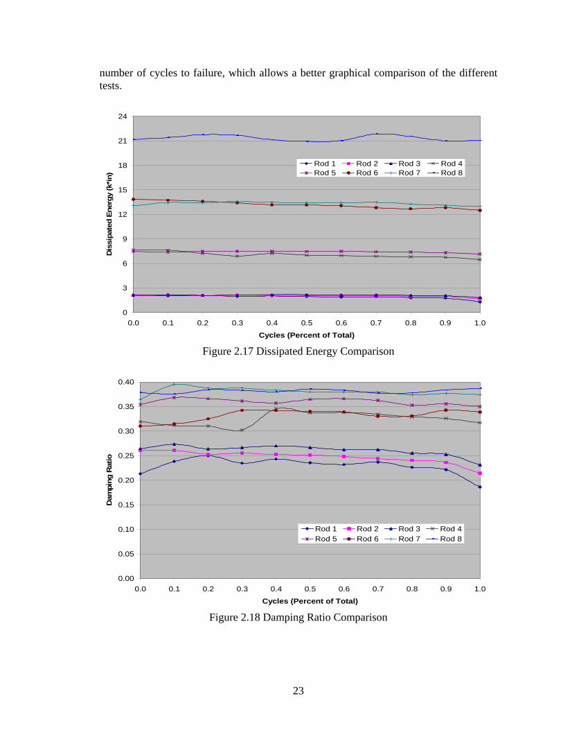
To ensure there is no degrading effect as the steel rods are subjected to cyclic
loading, the dissipated energy per cycle and the corresponding damping ratio and effective stiffness are plotted in Figure 2.17, Figure 2.18, and Figure 2.19 respectively, as a function of the number of loading cycles. The plots are normalized by their total
23
number of cycles to failure, which allows a better graphical comparison of the different tests.
0
3
6
9
12
15
18
21
24
0.0 0.1 0.2 0.3 0.4 0.5 0.6 0.7 0.8 0.9 1.0
Cycles (Percent of Total)
Dis
sipa
ted
Ener
gy (k
*in)
Rod 1 Rod 2 Rod 3 Rod 4Rod 5 Rod 6 Rod 7 Rod 8
Figure 2.17 Dissipated Energy Comparison
0.00
0.05
0.10
0.15
0.20
0.25
0.30
0.35
0.40
0.0 0.1 0.2 0.3 0.4 0.5 0.6 0.7 0.8 0.9 1.0
Cycles (Percent of Total)
Dam
ping
Rat
io
Rod 1 Rod 2 Rod 3 Rod 4Rod 5 Rod 6 Rod 7 Rod 8
Figure 2.18 Damping Ratio Comparison
24
0.0
0.5
1.0
1.5
2.0
2.5
3.0
3.5
4.0
4.5
5.0
0.0 0.1 0.2 0.3 0.4 0.5 0.6 0.7 0.8 0.9 1.0
Cycles (Percent of Total)
Effe
ctiv
e St
iffne
ss (k
ip/in
)
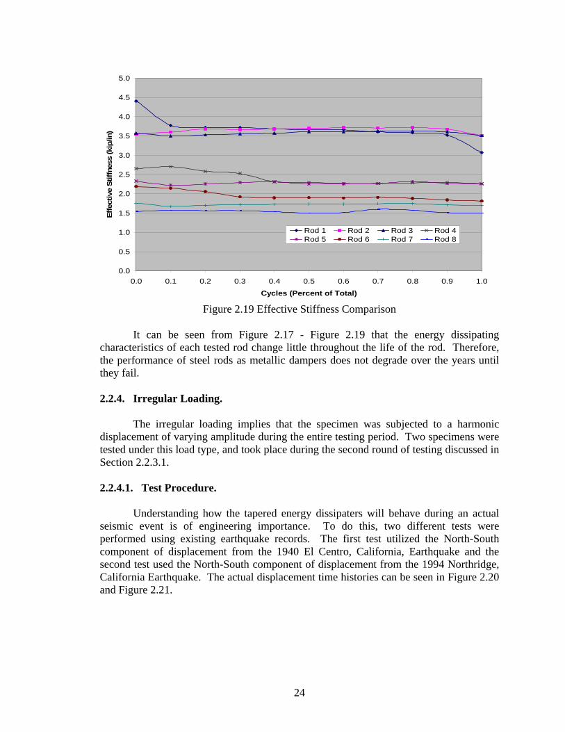
Rod 1 Rod 2 Rod 3 Rod 4Rod 5 Rod 6 Rod 7 Rod 8
Figure 2.19 Effective Stiffness Comparison
It can be seen from Figure 2.17 - Figure 2.19 that the energy dissipating
characteristics of each tested rod change little throughout the life of the rod. Therefore, the performance of steel rods as metallic dampers does not degrade over the years until they fail.
2.2.4. Irregular Loading.
The irregular loading implies that the specimen was subjected to a harmonic displacement of varying amplitude during the entire testing period. Two specimens were tested under this load type, and took place during the second round of testing discussed in Section 2.2.3.1.
2.2.4.1. Test Procedure.
Understanding how the tapered energy dissipaters will behave during an actual
seismic event is of engineering importance. To do this, two different tests were performed using existing earthquake records. The first test utilized the North-South component of displacement from the 1940 El Centro, California, Earthquake and the second test used the North-South component of displacement from the 1994 Northridge, California Earthquake. The actual displacement time histories can be seen in Figure 2.20 and Figure 2.21.
25
-1.2
-0.9
-0.6
-0.3
0.0
0.3
0.6
0.9
1.2
0 10 20 30 40 50 60
Time (sec)
Dis
plac
emen
t (in
)
Figure 2.20 Reduced Amplitude Displacement Time History of El Centro Earthquake
-1.2
-0.9
-0.6
-0.3
0.0
0.3
0.6
0.9
1.2
0 10 20 30 40 50 60
Time (sec)
Dis
plac
emen
t (in
)
Figure 2.21 Reduced Amplitude Displacement Time History of Northridge Earthquake
Since earthquake loads are basically random, it is anticipated that steel rods will
be subjected to cyclic loading of various amplitude sequences. Therefore, it was important to test the tapered energy dissipaters under a worst case type loading to ensure their ability will not be overestimated. By applying the largest sinusoidal displacements prior to the application of the smaller sinusoidal displacements the maximum amount of
26
damage is produced, therefore potentially reducing fatigue life. To represent a specific earthquake, however, the number of cycles corresponding to different displacement ranges from a peak to its following valley was counted.
Once the displacement plots shown in Figure 2.20 and Figure 2.21 had been
generated all maximum and minimum values for the plot were noted. From this information the range between each peak and valley was calculated. All of the range values were then modified to force the maximum range to become equal to 2.4", leading to a higher stress range than that induced by the actual earthquake. This was accomplished by multiplying each range value by a factor which was simply equal to 2.4" divided by the maximum range. This was done to study the effect of seismic waveform on the fatigue strength under the same earthquake intensity. The factor for each earthquake is then equal to aelcentro = 2.4"/max range = 2.4"/1.964" = 1.222, and anorthridge = 2.4"/max range = 2.4"/2.540" = 0.945.
The number of modified range values that fell into five different increments was
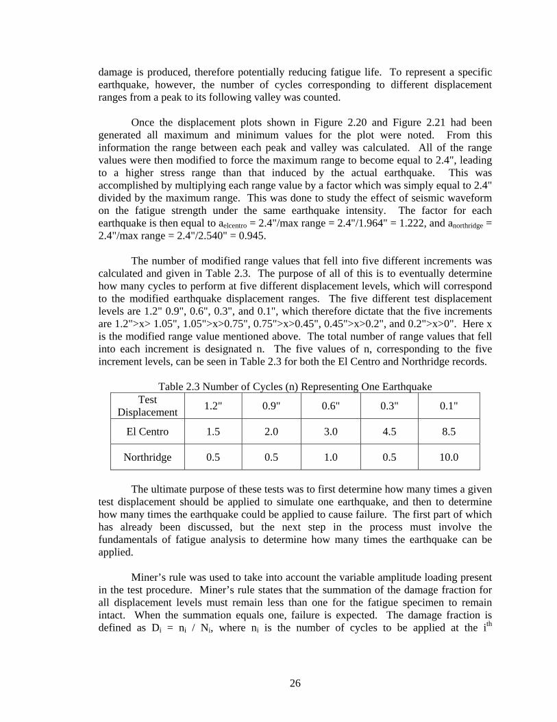
calculated and given in Table 2.3. The purpose of all of this is to eventually determine how many cycles to perform at five different displacement levels, which will correspond to the modified earthquake displacement ranges. The five different test displacement levels are 1.2" 0.9", 0.6", 0.3", and 0.1", which therefore dictate that the five increments are 1.2">x> 1.05", 1.05">x>0.75", 0.75">x>0.45", 0.45">x>0.2", and 0.2">x>0". Here x is the modified range value mentioned above. The total number of range values that fell into each increment is designated n. The five values of n, corresponding to the five increment levels, can be seen in Table 2.3 for both the El Centro and Northridge records.
Table 2.3 Number of Cycles (n) Representing One Earthquake Test
Displacement 1.2" 0.9" 0.6" 0.3" 0.1"
El Centro 1.5 2.0 3.0 4.5 8.5
Northridge 0.5 0.5 1.0 0.5 10.0
The ultimate purpose of these tests was to first determine how many times a given
test displacement should be applied to simulate one earthquake, and then to determine how many times the earthquake could be applied to cause failure. The first part of which has already been discussed, but the next step in the process must involve the fundamentals of fatigue analysis to determine how many times the earthquake can be applied.
Miner’s rule was used to take into account the variable amplitude loading present
in the test procedure. Miner’s rule states that the summation of the damage fraction for all displacement levels must remain less than one for the fatigue specimen to remain intact. When the summation equals one, failure is expected. The damage fraction is defined as Di = ni / Ni, where ni is the number of cycles to be applied at the ith
27
displacement level and Ni is the fatigue life in cycles at the same displacement. According to Miner’s Rule, the specimen is safe when
∑∑ <= 1i
ii N
nD (2.3)
Therefore, the number of times (m) the earthquake records needed to be applied to cause failure can be determined from
1*
"1.0"3.0"6.0"9.0"2.1
=⎥⎦
⎤⎢⎣
⎡⎟⎠⎞
⎜⎝⎛+⎟
⎠⎞
⎜⎝⎛+⎟
⎠⎞
⎜⎝⎛+⎟
⎠⎞
⎜⎝⎛+⎟
⎠⎞
⎜⎝⎛
Nn
Nn
Nn
Nn
Nnm
(2.4)
which has a representative term for the five test displacements. The calculation of the n values was found as discussed previously, but the calculation of the values for N was another matter.
The equation used to represent the S-N curve for steel can be written as
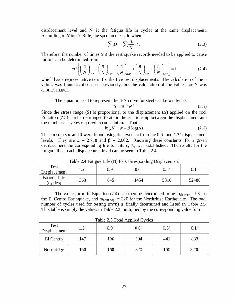
bC NS 10= (2.5) Since the stress range (S) is proportional to the displacement (∆) applied on the rod, Equation (2.5) can be rearranged to attain the relationship between the displacement and the number of cycles required to cause failure. That is, )log(log ∆−= βαN (2.6) The constants α and β were found using the test data from the 0.6" and 1.2" displacement levels. They are α = 2.718 and β = 2.002. Knowing these constants, for a given displacement the corresponding life to failure, N, was established. The results for the fatigue life at each displacement level can be seen in Table 2.4.
Table 2.4 Fatigue Life (N) for Corresponding Displacement Test
Displacement 1.2" 0.9" 0.6" 0.3" 0.1"
Fatigue Life (cycles) 363 645 1454 5818 52480
The value for m in Equation (2.4) can then be determined to be melcentro = 98 for
the El Centro Earthquake, and mnorthridge = 320 for the Northridge Earthquake. The total number of cycles used for testing (m*n) is finally determined and listed in Table 2.5. This table is simply the values in Table 2.3 multiplied by the corresponding value for m.
Table 2.5 Total Applied Cycles Test
Displacement 1.2" 0.9" 0.6" 0.3" 0.1"
El Centro 147 196 294 441 833
Northridge 160 160 320 160 3200
28
2.2.4.2. Results. After completion of the 833rd cycle at 0.1" for the El Centro displacement record,
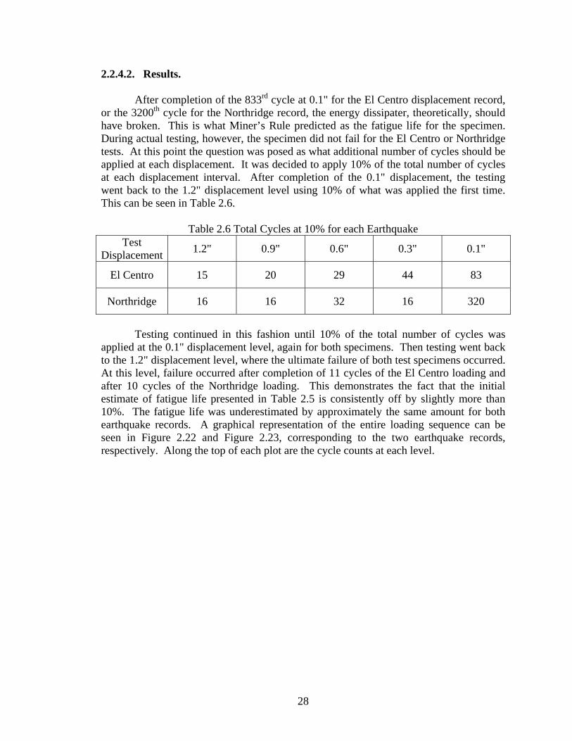
or the 3200th cycle for the Northridge record, the energy dissipater, theoretically, should have broken. This is what Miner’s Rule predicted as the fatigue life for the specimen. During actual testing, however, the specimen did not fail for the El Centro or Northridge tests. At this point the question was posed as what additional number of cycles should be applied at each displacement. It was decided to apply 10% of the total number of cycles at each displacement interval. After completion of the 0.1" displacement, the testing went back to the 1.2" displacement level using 10% of what was applied the first time. This can be seen in Table 2.6.
Table 2.6 Total Cycles at 10% for each Earthquake Test
Displacement 1.2" 0.9" 0.6" 0.3" 0.1"
El Centro 15 20 29 44 83
Northridge 16 16 32 16 320
Testing continued in this fashion until 10% of the total number of cycles was
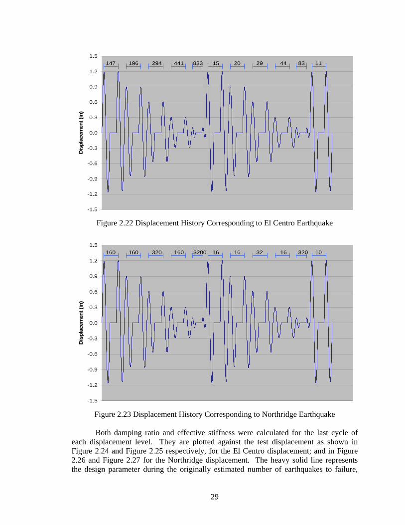
applied at the 0.1" displacement level, again for both specimens. Then testing went back to the 1.2" displacement level, where the ultimate failure of both test specimens occurred. At this level, failure occurred after completion of 11 cycles of the El Centro loading and after 10 cycles of the Northridge loading. This demonstrates the fact that the initial estimate of fatigue life presented in Table 2.5 is consistently off by slightly more than 10%. The fatigue life was underestimated by approximately the same amount for both earthquake records. A graphical representation of the entire loading sequence can be seen in Figure 2.22 and Figure 2.23, corresponding to the two earthquake records, respectively. Along the top of each plot are the cycle counts at each level.
29
-1.5
-1.2
-0.9
-0.6
-0.3
0.0
0.3
0.6
0.9
1.2
1.5
Dis
plac
emen
t (in
)
147 196 294 441 833 15 20 29 44 83 11
Figure 2.22 Displacement History Corresponding to El Centro Earthquake
-1.5
-1.2
-0.9
-0.6
-0.3
0.0
0.3
0.6
0.9
1.2
1.5
Dis
plac
emen
t (in
)
160 160 320 160 3200 16 16 32 16 320 10
Figure 2.23 Displacement History Corresponding to Northridge Earthquake
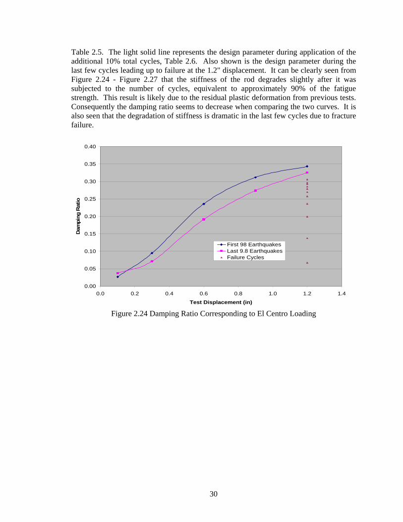
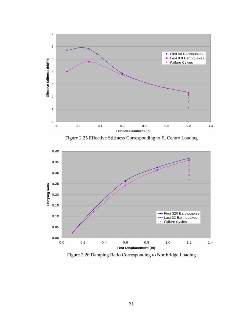
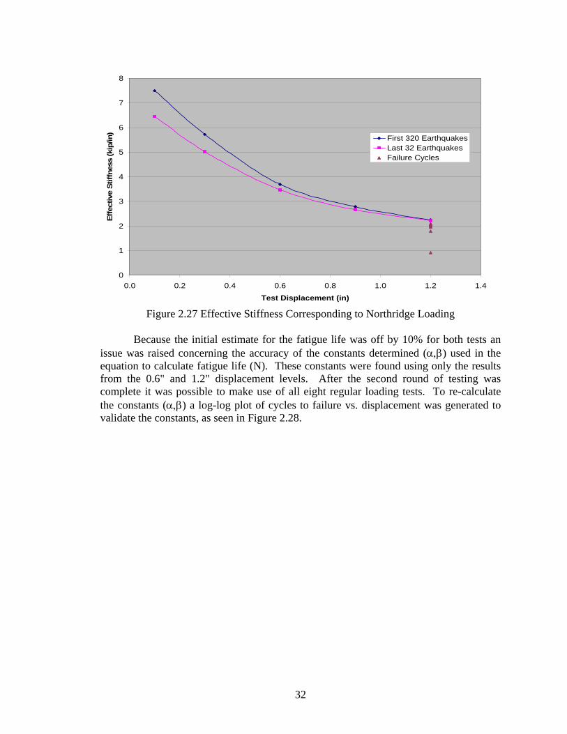
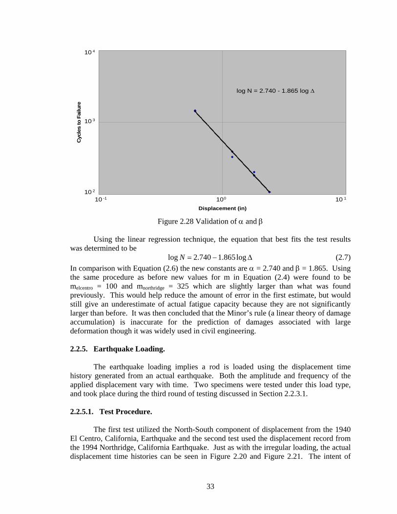
Both damping ratio and effective stiffness were calculated for the last cycle of
each displacement level. They are plotted against the test displacement as shown in Figure 2.24 and Figure 2.25 respectively, for the El Centro displacement; and in Figure 2.26 and Figure 2.27 for the Northridge displacement. The heavy solid line represents the design parameter during the originally estimated number of earthquakes to failure,
30
Table 2.5. The light solid line represents the design parameter during application of the additional 10% total cycles, Table 2.6. Also shown is the design parameter during the last few cycles leading up to failure at the 1.2" displacement. It can be clearly seen from Figure 2.24 - Figure 2.27 that the stiffness of the rod degrades slightly after it was subjected to the number of cycles, equivalent to approximately 90% of the fatigue strength. This result is likely due to the residual plastic deformation from previous tests. Consequently the damping ratio seems to decrease when comparing the two curves. It is also seen that the degradation of stiffness is dramatic in the last few cycles due to fracture failure.
0.00
0.05
0.10
0.15
0.20
0.25
0.30
0.35
0.40
0.0 0.2 0.4 0.6 0.8 1.0 1.2 1.4
Test Displacement (in)
Dam
ping
Rat
io
First 98 EarthquakesLast 9.8 EarthquakesFailure Cycles
Figure 2.24 Damping Ratio Corresponding to El Centro Loading
31
0
1
2
3
4
5
6
7
0.0 0.2 0.4 0.6 0.8 1.0 1.2 1.4
Test Displacement (in)
Effe
ctiv
e St
iffne
ss (k
ip/in
)
First 98 EarthquakesLast 9.8 EarthquakesFailure Cylces
Figure 2.25 Effective Stiffness Corresponding to El Centro Loading
0.00
0.05
0.10
0.15
0.20
0.25
0.30
0.35
0.40
0.0 0.2 0.4 0.6 0.8 1.0 1.2 1.4
Test Displacement (in)
Dam
ping
Rat
io
First 320 EarthquakesLast 32 EarthquakesFailure Cycles
Figure 2.26 Damping Ratio Corresponding to Northridge Loading
32
0
1
2
3
4
5
6
7
8
0.0 0.2 0.4 0.6 0.8 1.0 1.2 1.4
Test Displacement (in)
Effe
ctiv
e St
iffne
ss (k
ip/in
)
First 320 EarthquakesLast 32 EarthquakesFailure Cycles
Figure 2.27 Effective Stiffness Corresponding to Northridge Loading
Because the initial estimate for the fatigue life was off by 10% for both tests an
issue was raised concerning the accuracy of the constants determined (α,β) used in the equation to calculate fatigue life (N). These constants were found using only the results from the 0.6" and 1.2" displacement levels. After the second round of testing was complete it was possible to make use of all eight regular loading tests. To re-calculate the constants (α,β) a log-log plot of cycles to failure vs. displacement was generated to validate the constants, as seen in Figure 2.28.
33
Displacement (in)
Cyc
les
to F
ailu
re
log N = 2.740 - 1.865 log ∆
10 4
10 3
10 2
10 -1 100 10 1
Figure 2.28 Validation of α and β
Using the linear regression technique, the equation that best fits the test results
was determined to be ∆−= log865.1740.2log N (2.7) In comparison with Equation (2.6) the new constants are α = 2.740 and β = 1.865. Using the same procedure as before new values for m in Equation (2.4) were found to be melcentro = 100 and mnorthridge = 325 which are slightly larger than what was found previously. This would help reduce the amount of error in the first estimate, but would still give an underestimate of actual fatigue capacity because they are not significantly larger than before. It was then concluded that the Minor’s rule (a linear theory of damage accumulation) is inaccurate for the prediction of damages associated with large deformation though it was widely used in civil engineering. 2.2.5. Earthquake Loading.
The earthquake loading implies a rod is loaded using the displacement time
history generated from an actual earthquake. Both the amplitude and frequency of the applied displacement vary with time. Two specimens were tested under this load type, and took place during the third round of testing discussed in Section 2.2.3.1.
2.2.5.1. Test Procedure.
The first test utilized the North-South component of displacement from the 1940
El Centro, California, Earthquake and the second test used the displacement record from the 1994 Northridge, California Earthquake. Just as with the irregular loading, the actual displacement time histories can be seen in Figure 2.20 and Figure 2.21. The intent of
34
irregular loading was to simulate a worst-case type of loading condition for the earthquake record, but it is the purpose of this section to apply the actual earthquake record with modification of its amplitude only.
The displacement time record was generated with a HP E1415 control
workstation, including a HP1415A Algorithmic Closed Loop Controller, and a specialized computer program written for this study. In addition, the HP VEE visual program allowed real time viewing of the input. The displacement record was then used to drive the actuator, providing the load on each tested specimen. The time histories of the applied load, and the strain and displacement of the specimen were recorded during testing with the data acquisition unit, as shown in Figure 2.10.
2.2.5.2. Results.
The recorded displacement time histories are plotted in Figure 2.29 and Figure
2.30, respectively, for the El Centro and Northridge earthquakes. They are the same as those in Figure 2.20 and Figure 2.21 except a slightly reduced peak value due to the dynamics of the work station and the hydraulic actuator.
-1.2
-0.9
-0.6
-0.3
0.0
0.3
0.6
0.9
1.2
0 10 20 30 40 50 60
Time (sec)
Dis
plac
emen
t (in
)
Figure 2.29 Recorded Displacement Time History Corresponding to the 1940 El Centro
Earthquake
35
-1.2
-0.9
-0.6
-0.3
0.0
0.3
0.6
0.9
1.2
0 10 20 30 40 50 60
Time (sec)
Dis
plac
emen
t (in
)
Figure 2.30 Recorded Displacement Time History Corresponding to the 1994 Northridge
Earthquake
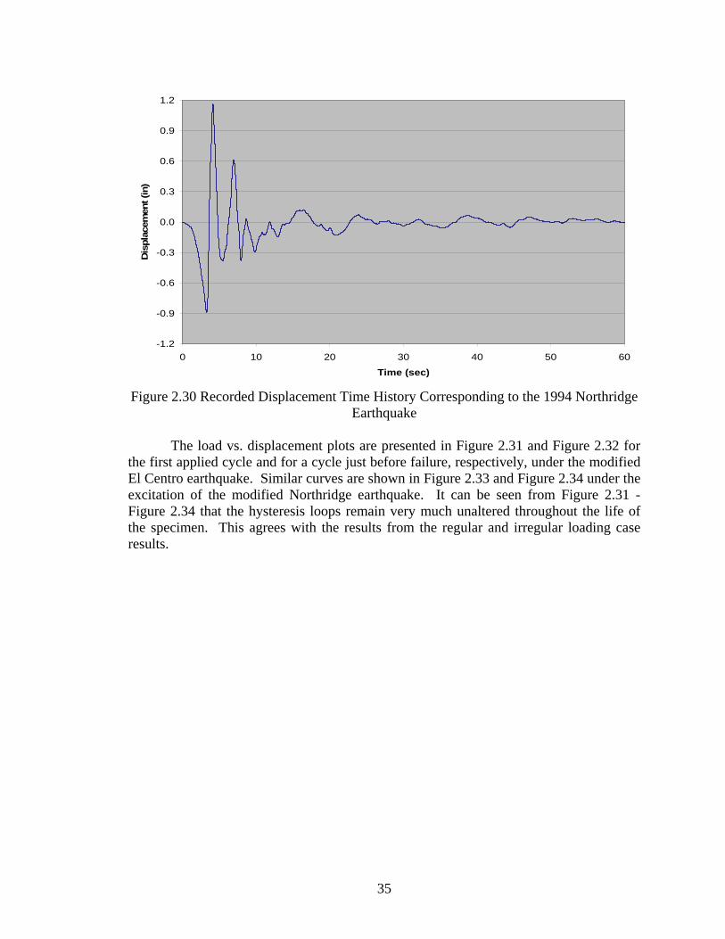
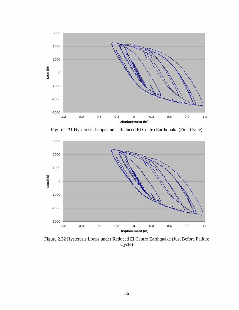
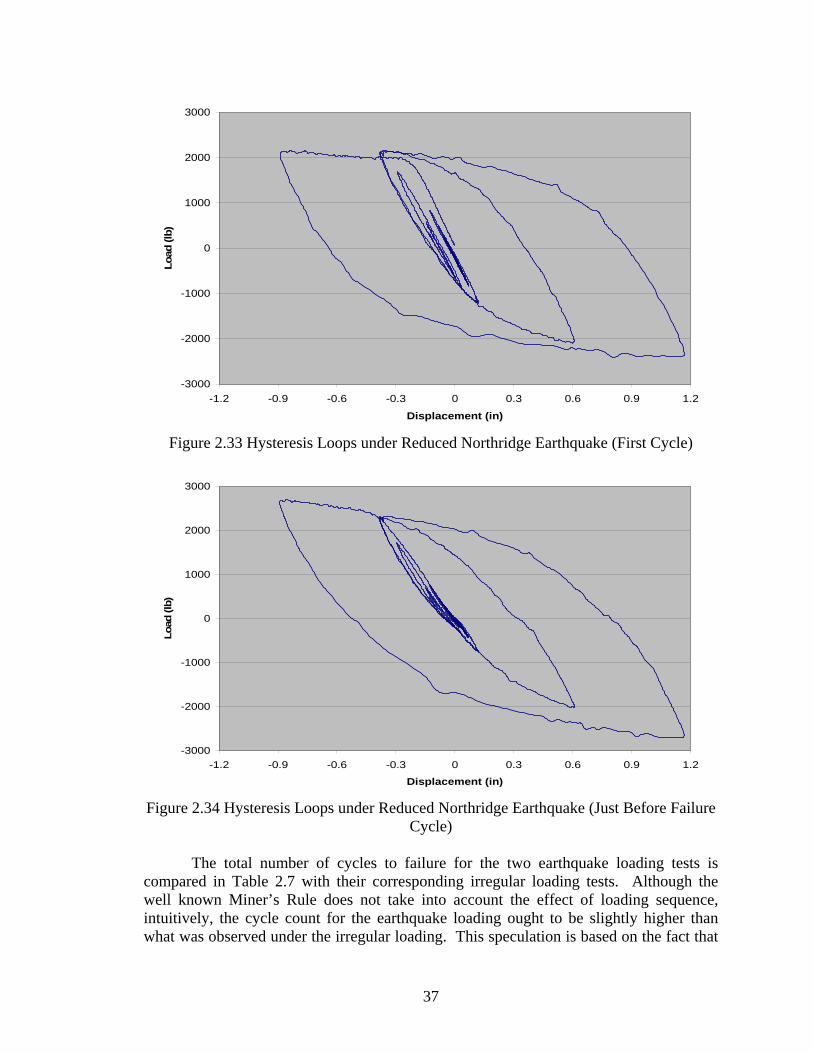
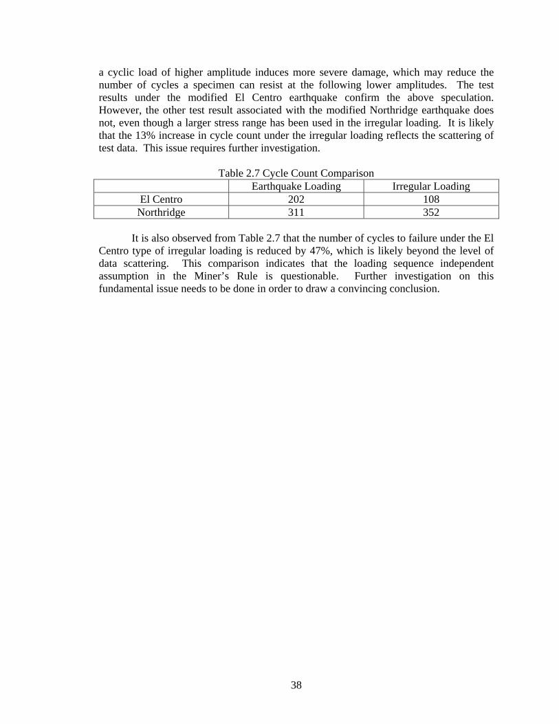
The load vs. displacement plots are presented in Figure 2.31 and Figure 2.32 for the first applied cycle and for a cycle just before failure, respectively, under the modified El Centro earthquake. Similar curves are shown in Figure 2.33 and Figure 2.34 under the excitation of the modified Northridge earthquake. It can be seen from Figure 2.31 - Figure 2.34 that the hysteresis loops remain very much unaltered throughout the life of the specimen. This agrees with the results from the regular and irregular loading case results.
36
-3000
-2000
-1000
0
1000
2000
3000
-1.2 -0.9 -0.6 -0.3 0 0.3 0.6 0.9 1.2
Displacement (in)
Load
(lb)
Figure 2.31 Hysteresis Loops under Reduced El Centro Earthquake (First Cycle)
-3000
-2000
-1000
0
1000
2000
3000
-1.2 -0.9 -0.6 -0.3 0 0.3 0.6 0.9 1.2
Displacement (in)
Load
(lb)
Figure 2.32 Hysteresis Loops under Reduced El Centro Earthquake (Just Before Failure
Cycle)
37
-3000
-2000
-1000
0
1000
2000
3000
-1.2 -0.9 -0.6 -0.3 0 0.3 0.6 0.9 1.2
Displacement (in)
Load
(lb)
Figure 2.33 Hysteresis Loops under Reduced Northridge Earthquake (First Cycle)
-3000
-2000
-1000
0
1000
2000
3000
-1.2 -0.9 -0.6 -0.3 0 0.3 0.6 0.9 1.2
Displacement (in)
Load
(lb)
Figure 2.34 Hysteresis Loops under Reduced Northridge Earthquake (Just Before Failure
Cycle)
The total number of cycles to failure for the two earthquake loading tests is compared in Table 2.7 with their corresponding irregular loading tests. Although the well known Miner’s Rule does not take into account the effect of loading sequence, intuitively, the cycle count for the earthquake loading ought to be slightly higher than what was observed under the irregular loading. This speculation is based on the fact that
38
a cyclic load of higher amplitude induces more severe damage, which may reduce the number of cycles a specimen can resist at the following lower amplitudes. The test results under the modified El Centro earthquake confirm the above speculation. However, the other test result associated with the modified Northridge earthquake does not, even though a larger stress range has been used in the irregular loading. It is likely that the 13% increase in cycle count under the irregular loading reflects the scattering of test data. This issue requires further investigation.
It is also observed from Table 2.7 that the number of cycles to failure under the El
Centro type of irregular loading is reduced by 47%, which is likely beyond the level of data scattering. This comparison indicates that the loading sequence independent assumption in the Miner’s Rule is questionable. Further investigation on this fundamental issue needs to be done in order to draw a convincing conclusion.
39
3. SEISMIC RETROFIT OF AN EXISTING HIGHWAY BRIDGE 3.1. Background
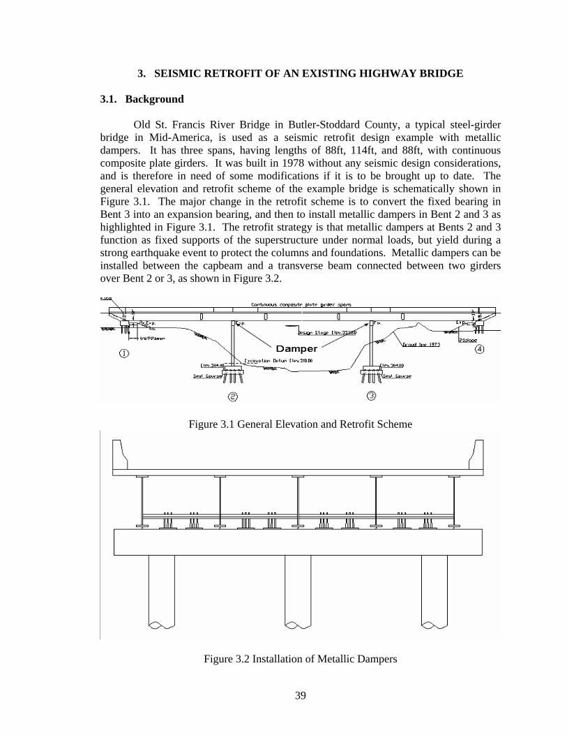
Old St. Francis River Bridge in Butler-Stoddard County, a typical steel-girder bridge in Mid-America, is used as a seismic retrofit design example with metallic dampers. It has three spans, having lengths of 88ft, 114ft, and 88ft, with continuous composite plate girders. It was built in 1978 without any seismic design considerations, and is therefore in need of some modifications if it is to be brought up to date. The general elevation and retrofit scheme of the example bridge is schematically shown in Figure 3.1. The major change in the retrofit scheme is to convert the fixed bearing in Bent 3 into an expansion bearing, and then to install metallic dampers in Bent 2 and 3 as highlighted in Figure 3.1. The retrofit strategy is that metallic dampers at Bents 2 and 3 function as fixed supports of the superstructure under normal loads, but yield during a strong earthquake event to protect the columns and foundations. Metallic dampers can be installed between the capbeam and a transverse beam connected between two girders over Bent 2 or 3, as shown in Figure 3.2.
Figure 3.1 General Elevation and Retrofit Scheme
Figure 3.2 Installation of Metallic Dampers
40
3.2. Design Procedure
The retrofit of a steel-girder bridge with metallic dampers can be designed using the ultimate strength method according to the following procedure summarized in Chen et al. (2001). The bridge was constructed with Class B1 Concrete with a compressive strength f’
c=4,000psi. The reinforcing steel used in the bridge has a yielding strength fy=40,000 psi, except for the reinforcing steel used in the superstructure slab and safety barrier curb which has a higher yielding strength of (Grade 60) fy=60,000 psi. A36 structural steel, having a yield stress of fy=36,000 psi, was used in the girders.
3.2.1. Loading.
The dead load of the bridge was based on the geometry and material properties
specified on the design drawings, and the HS20-44 live load from the AASHTO (1996) Standard Specification was considered in this example. The first value calculated was the total gravity load per column. This value is required to determine the plastic moment of the column, which is explained in Section 3.2.2. The second set of calculations required is the total mass of the deck and the total mass of the pier. These values are required to complete the response spectrum analysis to determine the maximum displacement of the bridge deck during excitation. This is discussed in Section 3.2.4. The contributing components to the total dead load include the following: concrete overlay, concrete slab, steel girder (web, flange, and stiffeners), bearings, capbeam, column, and the safety barrier curb.
3.2.1.1. Dead Load Per Column.
The calculations for the total dead load per column are now explained in detail.
lbftlblwtW coverlay 33180150'101'417.39
6'1
31
31
3 =∗∗∗∗=∗∗∗∗= γ (3.1)
lbftlblwtW cslab 161900150'101'75.42
4'3
31
31
3 =∗∗∗∗=∗∗∗∗= γ (3.2)
The weight contribution from the girders is first broken up into the weight from the web, flange, and the stiffeners. The flange and stiffeners have two different sizes along the length of the girder, which show up in the calculations.
lbftlblhtW sweb 8506490'101"66
8"3
3 =∗∗∗=∗∗∗= γ (3.3)
( )
lbftlb
lwtlwtW sflange
8943490'48"104"3'53"16
8"92
2
3
222111
=∗⎟⎠⎞
⎜⎝⎛ ∗∗+∗∗∗=
=∗∗∗+∗∗∗= γ (3.4)
( )
lbftlb
nwtnwthW sstiffeners
5.12094902"88"730"5.4
8"3"66
3
222111
=∗⎟⎠⎞
⎜⎝⎛ ∗∗+∗∗∗=
=∗∗∗+∗∗∗= γ (3.5)
41
The weight contribution of the girder is then approximately five times the sum of the individual contributions divided by three. This is simply because there are five girders and three columns supporting them.
( ) lbWWWW stiffenersflangewebgirder 3110035
=++∗= (3.6)
The total weight for all bearings present on the bridge was given as 7025lb. It is assumed that this weight is evenly distributed among the four bents.
lblbWbearing 4.585
47025
31
=∗=
(3.7)
lbftlblwhW ccapbeam 21000150'5.42'167.3'12.3
31
31
3 =∗∗∗∗=∗∗∗∗= γ (3.8)
( ) lbftlbhdW ccolumn 27920150'33.26'3
44 322 =∗∗∗=∗∗∗=
πγπ (3.9)
There are two safety barrier curbs located on the two sides of the bridge and it is assumed that their weight will be evenly distributed to each column.
lbftlbftlAW ccurb 44220150'101378.4
32
32
32 =∗∗∗=∗∗∗= γ (3.10)
The total dead load per column is then the sum of all contributions.
lbWWW
WWWWW
curbcolumncapbeam
bearinggirderslaboverlaydead
319900=+++
++++= (3.11)
kipWP deadcolumn 9.319== (3.12) 3.2.1.2. Total Mass. The calculations for the total mass of both the deck and pier are now explained in
detail.
lbftlblwtW coverlay 285800150'290'417.39
6'1
3 =∗∗∗=∗∗∗= γ (3.13)
lbftlblwtW cslab 1395000150'290'75.42
4'3
3 =∗∗∗=∗∗∗= γ (3.14)
The weight contribution from the girders is first broken up into the weight from the web, flange, and the stiffeners. The flange has two different sizes and the stiffeners have three different sizes along the length of the girder, which show up in the calculations.
lbftlblhtW sweb 24420490'290"66
8"3
3 =∗∗∗=∗∗∗= γ (3.15)
( )
lbftlb
lwtlwtW sflange
22380490'184"104"3'106"16
8"92
2
3
222111
=∗⎟⎠⎞
⎜⎝⎛ ∗∗+∗∗∗=
=∗∗∗+∗∗∗= γ (3.16)
( )
lbftlb
nwtnwtnwthW sstiffeners
34344904"5.58"54"8
8"784"5.4
8"3"66
3
333222111
=∗⎟⎠⎞
⎜⎝⎛ ∗∗+∗∗+∗∗∗=
=∗∗∗+∗∗+∗∗∗= γ (3.17)
42
The weight contribution of the girder is then five times the sum of the individual contributions because there are five girders supporting the deck. ( ) lbWWWW stiffenersflangewebgirder 2512005 =++∗= (3.18) There are two safety barrier curbs located on the two sides of the bridge and it is assumed that their entire weight contributes to the total weight of the deck.
lbftlbftlAW ccurb 380900150'290378.422 3
2 =∗∗∗=∗∗∗= γ (3.19)
The total mass of the deck includes contributions from the weight of the concrete overlay, concrete slab, steel girders, and the safety barrier curb.
( )
inkip
inlb
WWWWg
m curbgirderslaboverlayd
22 sec990.5sec5990
1
∗=
∗=
=+++∗= (3.20)
The total weight for all bearings present on the bridge is 7025lb. It is assumed that this weight is evenly distributed among the four bents. The two intermediate bents are fixed, due to the implementation of the damping units, and are therefore included in the analysis.
lblbWbearing 35132
7025== (3.21)
Again, both intermediate bents are included in the analysis therefore requiring the mass of both capbeams to be included in the total mass.
It is assumed that only the upper half of the column’s mass will contribute to the system during excitation. There are three columns at the two intermediate bents, totaling six, but only half of their mass is to be included in the analysis.
( ) lbftlbhdW ccolumn 83750150'33.26'3
43
4216 3
22 =∗∗∗∗=∗∗∗∗∗=πγπ (3.23)
The total mass of the pier includes the contributions from the weight of the bearings, capbeam, and columns.
( )in
kipin
lbWWWg
m columncapbeambearingp
22 sec552.0sec3.5521 ∗=
∗=++∗= (3.24)
3.2.2. Plastic Moment. Evaluate the longitudinal plastic moment (Mp) at the bottom of an existing fixed
pier. Once the plastic moment of the column is known an ultimate diameter for the damper can be established. This calculation is necessary to ensure that the damper yields prior to the formation of a plastic hinge at the column base of the fixed bent.
To evaluate the longitudinal plastic moment (Mp) at the column base of the fixed
bent the axial force on the pier resulting from gravity loads must be taken into account. The dead loads were considered to be evenly distributed on the three columns located at
43
each bent. The calculations for the gravity load per column can be found in Section 3.2.1.1.
Once the axial load on each column was known the corresponding plastic moment
could then be determined. Using the column cross section shown in Figure 3.3 and the material as well as geometric properties presented in Table 3.1, a trial-and-error solution could be generated assuming values for the depth of compression (c). When the assumed value for the compression depth output an axial load that corresponded to the actual gravity load on the column, the plastic moment that was calculated using this value of c was then accepted to be the plastic moment of the column.
Figure 3.3 Column Cross Section
In Table 3.1 the distances (d1 - d6) represent the distance from the compression
side of the column to different locations of the rebar, as illustrated in Figure 3.3 for d4 and d6.
Table 3.1 Material and Geometric Properties
psif c 4000' = "36=h
003.0=cuε "03.31 =d
ksif y 40= "04.72 =d
ksiEs 29000= "99.133 =d
85.01 =α "01.224 =d
85.01 =β "96.285 =d
22 54.227.1*2 ininAo == "97.326 =d
Again, the purpose of this iterative process is to determine the depth of the
compression block that will correspond to the gravity load on the columns. The axial force on a column due to dead loads calculated in Section 3.2.1.1, is Pcolumn = 319.9kip.
44
Different values for the compression block were used until a value of "377.9=c was found to correspond to the axial force, Pcolumn. Using this value for the compression block the iterative procedure used to calculate the plastic moment is shown as following.
The stress values at the location of the steel must first be calculated. The
magnitude of the stress in the steel cannot exceed the yielding stress which is set at fy = 40ksi.
ksifksiksicdc
Ef scuss 40;4088.58** 11
1 =>=−
= ε (3.25)
ksiksicdc
Ef cuss 4068.21** 22 <=
−= ε (3.26)
ksifksiksic
cdEf scuss 40;4080.42** 3
33 =>=
−= ε (3.27)
ksifksiksic
cdEf scuss 40;402.117** 4
44 =>=
−= ε (3.28)
ksifksiksic
cdEf scuss 40;407.181** 5
55 =>=
−= ε (3.29)
ksifksiksic
cdEf scuss 40;409.218** 6
66 =>=
−= ε (3.30)
The depth of the equivalent rectangular stress block (a) is needed to calculate the resulting force and plastic moment. The angle (θ) and the shaded area (A) in Figure 3.3 can be determined by "970.7*1 == ca β (3.31)
radh
ah
980.0)
2
2arccos( =−
=θ (3.32)
22 5.167)4
cos*sin(* inhA =−
=θθθ (3.33)
Once all parameters are calculated the resulting axial force on the column can be established. kipffffffAAfP ssssssoc 9.319)(**'* 6543211 =−−−−++= α (3.34) The corresponding plastic moment is then calculated as
ftkiphdfhdf
hdfdhfdhf
dhfAhAfM
ss
sss
socp
∗=−+−+
+−+−+−+
+−+−
=
1095)]2
(*)2
(*
)2
(*)2
(*)2
(*
)2
(*[*)cos*sin
)(sin*3
(**'*
6655
443322
11
3
1 θθθθα
(3.35)
It is of an utmost importance to design the metallic dampers in such a way as to make sure that they yield and dissipate energy before the column support structure of the bridge undergoes any permanent deformation. The moment required to cause yielding of
45
the dampers must be less than the plastic moment of the column. In this design, eight damping units or dampers are installed between the capbeam and the cross beam for each of the two intermediate bents, Figure 3.2, while three columns support each capbeam. Therefore the yielding force of each damper, Py, must be less than
kipftkipH
MPP p
yy 00.12'33.263.1
1095*83
**
83
max =∗
∗==<
α (3.36)
assuming that the longitudinal earthquake loads are only transferred through the damper. Here, H is the height of the fixed bent set at 26'-4" and α is the steel overstrength factor (1.3 in design) for the damper material. Then, the ultimate size of the damper can be determined from the maximum yielding strength Pymax and the required height. The derivation for the equation used to determine the diameter will now be discussed. First the height and yielding stress for the tapered rods must be defined. Based on the vertical clearance of the existing bridge and the results of tensile tests, they were selected as h = 16" and fy = 32ksi.
The steel rods were considered as cantilevered members, and the plastic section modulus of a circular rod can be expressed as
6
3dS p =
(3.37)
The diameter of the five rod metallic damper will be derived from hPfS yyp **5 =∗ (3.38) The ultimate diameter allowed that will guarantee yielding prior to the formation of a plastic hinge at the base of the column is then
"931.1**56
3 max ==y
yult fhPd (3.39)
A diameter smaller than the ultimate must be chosen, and the actual yielding force Py can then be found using a rearranged version of the same equation. A value of 1.9" was selected for use as the maximum diameter of the tapered rod.
The selected member size can be seen in Figure 3.4. The largest diameter along the tapered portion of the rod is 1.9", and it has a total height along the tapered section of 16.0". The smallest diameter along the tapered portion is set to 1.0" so that the maximum stress occurs approximately at the middle height of the rod. This is derived as follows.
46
Figure 3.4 Selected Member for Retrofit Design
The force required to cause yielding at the extreme fiber of the tapered rod (Py) is
a function of the yielding stress of the steel, the location of maximum stress (xmax), and the diameter at the location of maximum stress (dmax). To aid in the derivation of the above relation, the tapered portion of the rod is idealized as a circular, cantilevered beam as shown in Figure 3.5.
47
Figure 3.5 Cantilever Section
At a distance x from the top, the moment on the cantilever beam and the section
modulus of the circular section are respectively equal to M(x) = P*x and S(x) = π*d3(x)/32, in which d(x) = 1+0.056*x. The stress at the extreme fiber of any given location is given by
)(
32)()()( 3 xd
xPxSxMx
∗∗∗
==π
σ (3.40)
The location of the maximum stress, xmas, is obtained when σ(x) is a maximum. By setting the first derivative of σ(x) equal to zero, xmax was found to be xmax = 8.889", and the diameter at the location of maximum stress was known to be "50.1"889.8056.01max =∗+=d . (3.41) Then by substituting fy into the stress equation, the yielding force can be expressed into
rodkipksixdf
P yy /193.1
"889.832)"5.1(32
32)( 3
max
3max =
∗∗∗
=∗
∗∗=
ππ (3.42)
3.2.3. Longitudinal Forces. Check for the longitudinal forces due to non-seismic loads. Yielding of the
metallic dampers under typical non-seismic forces is not desired. In order to make sure there will not be any problems the inequality
∑<∗ yPQmaxβ (3.43)
must be met, where Qmax is the maximum longitudinal force of all load combination in AASHTO specification (1996) due to non-seismic loads and β is a factor used to ensure the damper behaves elastically under non-seismic loads. This should be determined during consultation with the bridge owner, and for this study β = 1.3. In Equation (3.43), ΣPy represents the total yielding force of all dampers. The yielding force of each damper of five rods is Py = 5*1.193 = 5.965kip from Equation (3.42).
48
According to AASHTO specification (1996), Article 3.9, provision shall be made for the effect of a longitudinal force of five percent of the live load in all lanes carrying traffic headed in the same direction. The load used shall be the lane load plus the concentrated load for moment specified in Article 3.7, with reduction for multiple-loaded lanes as specified in Article 3.12. The center of gravity of longitudinal force shall be assumed to be located six feet above the floor slab and to be transmitted to the substructure through the superstructure. In the retrofit design of bridges with metallic dampers, the dampers will take the longitudinal force. The total longitudinal force Qmax is
( )( ) lbQ 211602881148864026000%5max =∗++∗+∗= (3.44) 16 dampers are installed in the two lanes to resist the longitudinal force. kipkipQ 44.95965.516P1627.51kip21.16kip1.3* ymax =∗=∗≤=∗=β (3.45) The maximum longitudinal force is well below the yielding force of the damping units; therefore typical non-seismic forces will not pose a problem. 3.2.4. Maximum Displacement.
Evaluate the maximum displacement of the superstructure under a design
earthquake. Since the Old St. Francis Bridge has a fundamental natural period of 1.32 sec., (Anderson et al. 2001) the bridge structure is relatively flexible, particularly when the metallic dampers are installed. Therefore, the bridge and damper system can be analyzed as an equivalent, linear two-degree-of-freedom system with the response spectrum method. The motion of deck and capbeam are considered the degrees of motion as schematically illustrated in Figure 3.6. The stiffness and damping coefficients, kd and cd, are from the metallic dampers to be installed on the bridge.
Figure 3.6 Two-Degree-of-Freedom Model of Bridge and Damper System
49
For this analysis the bearings are considered as ideal roller or pin supports. A response spectrum analysis was performed on the structure to estimate the maximum displacement that would occur under the El Cento earthquake. Before the response spectrum analysis could be performed a few constants had to be established, which included the mass, stiffness, and damping coefficient of the deck, and pier. The calculation of the two mass values can be seen in Section 3.2.1.2, but the results are now summarized.
inkipmd
2sec*990.5=
(3.46)
inkipm p
2sec*552.0=
(3.47)
Referring to Table 3.1 for the compressive strength of the concrete and diameter of the column, the stiffness of one column ko can be computed as follows ksipsifE cc 605,3000,605,3'*57000 === (3.48)
44
8245064* indI ==
π (3.49)
inkip
HIE
k co 27.28
**33 == (3.50)
inkipkk op 62.169*6 == (3.51)
The damping coefficient, cp, can be estimated with a simplified model as shown
Figure 3.7 after all dampers are assumed to function as hinges. In this case, the natural frequency of the pier could be determined, and an assumption that the damping ratio of the pier was equal to five percent allowed the damping constant for the pier to be calculated.
sec
158.5 radmm
k
dp
pp =
+=ω (3.52)
05.0=pξ (3.53)
in
kipmmc pdpppsec*288.3*)(**2 =+= ωξ (3.54)
Figure 3.7 Model of Bridge for Longitudinal Stiffness
50
Now, the only remaining constants required for the response spectrum analysis were the stiffness and damping coefficients of the damper. Both the secant stiffness and damping ratio for the damper are functions of the maximum displacement that the damper will undergo during the El Centro excitation. Therefore in order to calculate the maximum displacement using a response spectrum analysis, the maximum displacement first had to be known. As a result, the process was an iterative one.
Since the specimens tested in Section 2 are smaller than that for the bridge
retrofit, their test results may not be applicable to the rod in Figure 3.4. Therefore, numerical analysis with ABAQUS software was performed to facilitate the determination of stiffness. In order to test the validity of numerical results found using ABAQUS a finite element model was created that exactly matched the test specimens size and shape, seen in Figure 2.7(a), and an analysis was performed to see how closely the results given by ABAQUS resembled the actual test results, given in Table 2.2. ABAQUS proved to give accurate results as they corresponded to test results with little discrepancy. This topic is further discussed in Section 3.3. After ABAQUS results were verified, the analysis of the rod in Figure 3.4 can be performed and the corresponding results could be used to determine the effective stiffness.
In order to calculate the tapered rods stiffness an arbitrary load was placed at the
top of the member and the maximum displacement was computed. The effective stiffness at this loading level was then simply the load value applied divided by the corresponding displacement. This stiffness was multiplied by the total number of rods that were to be installed and a total stiffness was known. Whether or not this was the correct stiffness value would not be known until after the response spectrum analysis was performed using this value. If the response spectrum analysis output a maximum displacement that was exactly the displacement from which the member stiffness was calculated, then and only then was the stiffness value and maximum displacement value used known to be correct. If the response spectrum analysis output a maximum displacement that was not equivalent to the displacement from which the member stiffness was calculated then the process started over. A different load was applied to the model in ABAQUS, different maximum displacement and stiffness values were found, and the response spectrum analysis was performed again. This continued until the displacement values corresponded.
Once the actual stiffness and maximum displacement were determined for a rod
with given dimensions, it still would not necessarily be an acceptable solution. There were restraints placed on the maximum displacement that the bridge deck can move, due to the limitations of the expansion joints. This limited the maximum displacement of the bridge to roughly 2.5". Any rod allowing the superstructure of the bridge to have a displacement larger than this was therefore found unsatisfactory for this design.
The response spectrum analysis calculations can be seen below for the selected
member size, Figure 3.4. Using ABAQUS a load of 3.1 kip was applied to the specimen and a maximum displacement of approximately 2.0" was generated. With this information and knowing a total of 80 rods are to be used, the total secant stiffness can be
51
found to be kd = 125 kip/in. The natural frequency was then established for the given stiffness as sec568.4 radmk ddd ==ω .
To determine the damping coefficient of steel rods, it is assumed that the damping
ratio, determined in Equation (2.2), is independent of the size of the rods. The assumption will be validated with the full-scale damper test in Section 4.4. Under this assumption, the test results in Table 2.2 were used to develop a regression curve between damping ratio and maximum displacement for extrapolation to determine the damping ratio corresponding to other displacements. Figure 3.8 shows the test data from Table 2.2 and a regression curve that best fits the data. The regression curve can be described by 0617.07969.05595.01674.00169.0 234 −∆∗+∆∗−∆∗+∆∗−=dξ (3.55) where ∆ is defined as the displacement under consideration. The yielding displacement of the rods (∆y), shown in Figure 3.8, is equal 0.082", which follows a calculation similar to the one to be summarized by Equation (3.78).
From Equation (3.55), the damping ratio corresponding to a maximum displacement of 2” was then found to be ξd = 0.36 and thus
in
kipmc ddddsec*70.19***2 == ωξ
(3.56)
The stiffness, damping, and mass matrices of the bridge-damper system can then be written as
[ ] ⎥⎦
⎤⎢⎣
⎡+−
−=
dpd
dd
kkkkk
K,
[ ] ⎥⎦
⎤⎢⎣
⎡+−
−=
dpd
dd
ccccc
C,
[ ] ⎥⎦
⎤⎢⎣
⎡=
p
d
mm
M0
0 (3.57)
52
The undamped natural frequencies of the system can then be calculated from the following characteristic equation [ ] [ ] 0*det 2 =− MK nω (3.58)
sec437.31 radn =ω , sec30.232 radn =ω . (3.59) Their corresponding mode shapes can be solved from [ ] [ ]( ) { } 0**2 =− nn MK φω (3.60)
{ }⎭⎬⎫
⎩⎨⎧
=398.0917.0
1φ , { }⎭⎬⎫
⎩⎨⎧−
=1
04.02φ . (3.61)
The damping ratio for the two modes can approximately be calculated as
{ } [ ] { }
{ } [ ] { } nnT
n
nT
nn M
Cωφφ
φφξ
****2**
= (3.62)
166.01 =ξ , 942.02 =ξ . (3.63) The modal participation factor is a term that measures the degree to which the nth mode participates into the total response of the structure.
{ } [ ] { }{ } [ ] { }n
Tn
Tn
n MIM
φφφ
γ****
= (3.64)
115.11 =γ , 557.02 =γ (3.65) As the results suggest, the first mode is more dominant than the second. According to Figure 6.6.4 in the textbook by Chopra (2001), the displacement spectral values corresponding to the natural frequency and modal damping ratio are "45.31 =dS and "10.02 =dS . (3.66) The maximum displacement between the bridge deck and capbeam can be expressed into "997.1)](**[)](**[ 2
2212222
211111max =−+−=∆ φφγφφγ dd SS . (3.67)
This value for the maximum displacement corresponds to the assumed deformation of the steel rods at the beginning of iteration, which was used in ABAQUS to determine the damper secant stiffness. This means that during the El Centro earthquake, with the implementation of 80 dampers having the dimensions of Figure 3.4, the bridge deck will be displaced approximately 2.0".
The maximum displacement corresponding to an AASHTO response spectrum
analysis (AASHTO 1996) must be checked to ensure that the El Centro response spectrum design does not underestimate the site response by any significant amount. The difference in the two methods is in the calculation of the displacement spectral values. Values such as the natural frequencies and damping ratios will remain the same.
Using the peak acceleration coefficient map, the location of the Old St. Francis
River Bridge (36.8°N, 90.2°W) has a value of A = 0.15. Considering the limited boring data (Anderson et al. 2001) the soil profile can be classified as either Type I or II. The following calculation will include the results for Type I, which dictates the site coefficient to be S = 1.0. The natural periods for the first two modes are
53
sec828.1437.322
11 ===
πω
π
n
T (3.68)
sec2697.030.23
22
22 ===
πω
π
n
T (3.69)
The corresponding elastic seismic response coefficients are calculated below, while ensuring their magnitudes do not exceed a value of 2.5A = 0.375.
( ) ( )
AT
SACs 5.21204.0sec828.1
0.115.02.12.1
32
32
1
1 <=∗∗
=∗∗
= (3.70)
( ) ( )
375.0;5.24312.0sec2697.0
0.115.02.12.12
32
32
2
2 =>=∗∗
=∗∗
= ss CAT
SAC (3.71)
Because these values are based on ξ = 5%, a reduction factor must be introduced before the spectral displacement values are determined. This will take into account the actual damping ratios for the first two modes. Chopra (2001) presents this equation as
( )( )
( )( ) 7661.05ln27.082.1
6.16ln27.082.15ln27.082.1
ln27.082.1 11 =
−−
=−−
=ξ
RF (3.72)
( )( )
( )( ) 4278.05ln27.082.1
2.94ln27.082.15ln27.082.1
ln27.082.1 22 =
−−
=−
−=
ξRF (3.73)
The spectral displacement values are
( ) ( )
( )"014.3
sec437.3sec3861204.0
7661.0 2
2
21
112
1
111
=⎥⎥⎦
⎤
⎢⎢⎣
⎡ ∗∗=
=⎥⎥⎦
⎤
⎢⎢⎣
⎡ ∗∗=
⎥⎥⎦
⎤
⎢⎢⎣
⎡∗=
radin
gCRF
SRFS sa
d ωω (3.74)
( ) ( )
( )"1141.0
sec30.23sec386375.0
4278.0 2
2
22
222
2
222
=⎥⎥⎦
⎤
⎢⎢⎣
⎡ ∗∗=
=⎥⎥⎦
⎤
⎢⎢⎣
⎡ ∗∗=
⎥⎥⎦
⎤
⎢⎢⎣
⎡∗=
radin
gCRF
SRFS sa
d ωω (3.75)
and the maximum displacement is ∆max = 1.745", using the same combination rule as in Equation (3.67). Therefore, the maximum displacement corresponding to the AASHTO response spectrum for a Type I soil is significantly smaller than what was estimated with the El Centro response spectrum. Even under the assumption that the soil is Type II, the maximum displacement is calculated to be ∆max = 2.093", which is close to the El Centro estimate. 3.2.5. Ductility.
Design for sufficient ductility. The displacement ductility demand is determined
by
54
y
d ∆∆
= maxµ (3.76)
where ∆max = 1.997" and ∆y is the yielding displacement of the damper. The recommended value for the ductility ratio is set to be 12 for low carbon steels. The calculation of the Ductility Demand can be seen below.
The conjugate beam method of structural analysis was used to determine the yielding displacement of each tapered rod as illustrated in Figure 3.5. The underlying principle of this method states that when the conjugate beam is loaded with the M(x)/EsI(x) diagram of the real beam the bending moment at any point on the conjugate beam equals the displacement on the real beam. Here I(x) is the moment of inertia of a circular cross section. In this case the real beam is the steel rod and its M(x)/EsI(x) equals
64)(29000)(
)(4 xd
xPxIE
xM y
x ∗∗
∗=
∗ π (3.77)
The yielding displacement (∆y) is equal to the moment at the fixed end of the conjugate beam, which at the free end of the real cantilevered beam can be determined by
"167.0)(**125.453
*)(*
)(
04
2
0
==∗=∆ ∫∫h
yh
sy dx
xdxP
xdxxIE
xMπ
(3.78)
in which Py = 1.193 kip/rod from Equation (3.42), h = 16", and d(x) = 1+0.056*x. Finally, the ductility demand is equal to
97.11max =∆
∆=
ydµ (3.79)
The ductility demand is within the target value of 12. Therefore this member size passes the ductility requirements set forth. 3.2.6. Rocker Bearing Capacity.
Check the ultimate capacity of the rocker bearings and verify the load distribution between dampers and rocker bearings. During a strong earthquake the bridge expansion bearings may behave non-linearly due to friction forces that may exist between the moving parts in the expansion bearings. For a full non-linear dynamic analysis of a bridge system a hysteretic model of each bearing needs to be developed. This is thoroughly discussed in Section 5, but the results are summarized here.
The Type D rocker bearings, received from two demolished bridges, were tested
in the laboratory by Barker and Hartnagel (1997). Test results show that Type D bearings are likely to become unstable when they are exposed to an ultimate displacement greater than 4.5”. The dampers will therefore yield and dissipate energy substantially before the rocker bearings will become unstable. For simplification, retrofit design in this section did not take into account the friction effect of the expansion bearings. This can be justified by the following considerations. First of all, the seismic retrofit of a highway bridge is often part of a deck rehabilitation project. As a result, existing bearings can either be replaced or cleaned during the deck replacement. Secondly, the friction of each
55
bearing typically ranges from 5 to 10 kips as can be seen from Section 5. Considering a total of 20 bearings and 16 dampers, the difference between the damper force, corresponding to the yielding of columns, and the yielding of the damper itself, equal to 11.93-5.965 = 5.965 kip/damper unit, can roughly overcome the friction of each bearing without transferring a significant amount of force from the bridge superstructure to the columns, thus denying the formation of a plastic hinge in the columns. This is especially true when the overstrength factor of the column section is considered. The rocker bearing capacity is not an issue for the Old St. Francis River bridge.
3.3. Non-Linear Analysis of Tapered Rods – ABAQUS
The calculation of the inelastic displacement of a linearly tapered rod required the use of a design software package that had the capability of performing non-linear analysis. Determining the stiffness of a tapered rod is quite difficult when the member is no longer deforming in the elastic range. As the amount of inelastic deformation increases the relative stiffness decreases. The design software selected to perform this analysis was ABAQUS, but could have been any program with similar abilities.
Validation of the results found using ABAQUS had to take place before the
results could be entirely trusted. Therefore, a model was created in ABAQUS, Figure 3.9, that exactly matched the previously tested specimens size and shape, Figure 2.7. Figure 3.9 displays both the undeformed and the deformed shapes. The mesh, used for the finite element analysis, and the stress contours are visible within the deformed shape. The mesh was created with 16 seeds around the diameter and 30 seeds longitudinally, which created 674 nodes and 2311 linear tetrahedral elements. The material was defined with E = 29000ksi and ν = 0.3, following the k2-adjusted stress-strain relation shown in Figure 2.3.
56
(a) Undeformed Shape (b) Deformed Shape
Figure 3.9 Finite Element Model of One Steel Rod
An analysis was performed to see how closely the results given by ABAQUS resembled the actual effective stiffness results. Both the test data from Table 2.2 and the numerical simulation results are presented in Figure 3.10. It is clearly seen from Figure 3.10 that, for a given displacement, the corresponding effective stiffness value from ABAQUS is accurate. Therefore, the analysis of any member with varying dimensions could be performed with a similar ABAQUS model and the corresponding results can be used for design.
57
0.0
0.5
1.0
1.5
2.0
2.5
3.0
3.5
4.0
4.5
0.0 0.5 1.0 1.5 2.0 2.5 3.0
Displacement (in)
Effe
ctiv
e St
iffne
ss (k
/in)
Test DataSimulation Data
Figure 3.10 Effective Stiffness of the Tested Specimens
3.4. Design Summary and Cost
Eight sets of five rods, each shown in Figure 3.4, will be implemented on each of two intermediate bents of the Old St. Francis River Bridge, making a total of 80 rods for the design. This is an economical solution for the seismic retrofit of the bridge. The material and labor cost of one damper unit was $1878 based on the quota for this research project, which included 5 rods and the base plate, Figure 4.1. The material and labor cost associated with the purchase of 16 damper units was $27,052, which includes a decrease in cost per unit due to ordering in bulk. All estimates were based on August 2004 steel prices which may vary from month to month.
This design procedure shows that the retrofit of highway bridges with metallic
dampers can be implemented into common practice. By following the same detailed procedure an economical solution can be generated for any existing steel girder bridge as long as it can meet all the requirements of retrofit design.
58
4. VALIDATION OF THE FULL SCALE METALLIC DAMPER 4.1. Background
Following completion of the seismic retrofit design for the existing bridge in Butler Stoddard County, the need to test this system was of great concern. The system refers to, not only the metallic dampers, but also to the other components necessary for the actual implementation of the damper into the bridge. The transverse beam, used as a direct link between the dampers and the bridge deck, and the bolted connection of the transverse beam to the existing bridge girders are two primary points of interest for the full scale test.
The retrofit design for the existing bridge under consideration provided the exact
size and number of metallic dampers that would be required for the structures survival. This was discussed in Section 3. There are to be eight dampers of five rods on each of two intermediate bents. For testing purposes, the “full scale” refers to one of these sets of five rods. Testing one group provides the information required to validate the rod’s energy dissipating abilities, but also the sufficiency of the connection. The actual rod size can be seen in Figure 3.4, but the five rod arrangement can be seen in Figure 4.1. This figure includes the layout of the base plate. This includes the dimensions for the bolt hole pattern, which match the existing pattern on the push beam to which it will be bolted.
59
Figure 4.1 Five Rod Specimen
4.2. Test Setup
For this study, tests were set up using the structural steel framework, located in
the structures lab at UMR, which had previously been purchased for other projects. A schematic drawing of both a top view and side view of the entire setup can be seen in Figure 4.2. Within the sketch, the locations of important components are designated for further reference. The actual overall test setup can be seen in Figure 4.3, but the actuator, which is connected to the left side of the push beam, cannot be seen in this photo. A better view of the actuator can be seen in Figure 4.4.
60
Figure 4.2 Test Setup Schematic
Damper Location
Damper Location
61
Figure 4.3 Overall Test Setup
Figure 4.4 Actuator
62
When on an actual bridge the base of the tapered dampers will be held fixed to the
top side of the capbeam and the cantilevered top ends will be inserted through the web of the transverse beam. As the superstructure of the bridge deck moves against the capbeam during an earthquake the transverse beam, being directly connected to the superstructure, experiences displacement with respect to the capbeam. As a result, the dampers installed between the transverse beam and the capbeam yield and dissipate energy. The test setup used this same longitudinal motion, but instead of the base being held fixed and the top undergoing the displacement, the top was held fixed and the base was displaced for convenience. The top of the rods were still freely rotating cantilevers, but their relative position did not change.
The fixed end of the 110-kip capacity hydraulic actuator is bolted in a horizontal
position to a beam that spans the gap between two columns. The actuator applies the sinusoidal load to the tapered specimens, representative of the earthquake induced motion. The load from the actuator to the specimens is transferred through a large beam, referred to as the push beam. The base of the five rod specimen is directly connected to the existing bolt hole pattern on the push beam, but the specimens are bolted upside down underneath the push beam. The motion of the push beam is completely limited to ensure only the desired motion is allowed. There are restraints placed to resist the vertical motion of the beam, which can be seen in Figure 4.3. The push beam is welded to roller plates, which not only give a frictionless plane for the beam to slide on, but they also restrict the horizontal motion of the push beam. Only longitudinal motion is allowed.
The tops of the rods are inserted through the web of the transverse beam, which is
held fixed by a shear connection to columns on either side. For testing purposes, ball joints were welded into the web of the transverse beam to house the top ends of the dampers. This ball joint connection gives a smoother connection between the two components, which allow enhanced performance of the damper. This connection can be seen in Figure 4.5 with a close up in Figure 4.6. The actuator sends the push beam in the longitudinal direction with a predetermined displacement, the base of the specimens move with the beam, and the top of the rods are held in a fixed position due to restraint from the transverse beam. A closer view of how the push beam, five rod damper, and transverse beam interact can be seen in Figure 4.7.
63
Figure 4.5 Ball Joint Connections
Figure 4.6 Ball Joint Close Up
64
Figure 4.7 Test Components Interaction
The reasoning behind why the five rod damping unit was bolted underneath the push beam, instead of on top, is simply to create a smaller moment when the load from the transverse beam is transferred into the column supports. The transverse beam connecting to the column supports at the lowest possible position creates the smallest possible moment, and correspondingly the smallest possible displacement of the column supports. This is desired to ensure the five rod specimen will undergo the total intended displacement without the top of the rods moving due to movement from column deflection. The less deflection the columns supporting the transverse beam have the closer the results will be to the field installation.
A total of twelve strain gauges were applied along the length of various members
in the plane of bending. The load applied was measured by an internal load cell within the actuator. The displacement of the system was measured using two different means; an internal LVDT included in the actuator and an external LVDT that was directly connected to the end of the push beam. Even though the transverse beam was economically designed to allow a miniscule amount of deflection during loading, the actual amount of deflection was measured using an external LVDT. In order to take this into account, during analysis this deflection is subtracted off of the total deflection. All data was recorded at 64 data points per second by a data acquisition unit, which can be seen in Figure 2.10. A side view of the test setup can be seen in Figure 4.3, but another view of the test setup can be seen in Figure 4.8. For a better view of the overall setup, this figure shows the test setup in the longitudinal direction without the vertical restraints on the push beam. The external LVDT is in line with the push beam and can be seen at the bottom of Figure 4.8.
65
Figure 4.8 Longitudinal View of Incomplete Test Setup 4.3. Test Apparatus
The damper was tested under a harmonic displacement of 2.0", 2.5", and 3.0".
The 2.0" displacement was determined because the maximum displacement the superstructure of the Old St. Francis River Bridge would move is approximately 2.0" under the El Centro Earthquake. In the case of a larger earthquake, the damper will likely experience a larger displacement. Therefore, displacements of 2.5" and 3.0" were to be applied after the application of the 2.0" displacement. The test protocol was to test the damper for 100 cycles at the 2.0" displacement, another 100 cycles at 2.5" displacement, and finally to the failure of all five rods at 3.0" displacement. A graphical representation of this loading protocol can be seen in the results section in Figure 4.16.
Before testing of the damper could take place, other necessary components had to
first be designed. The two components designed that would be required for the actual bridge included the transverse beam and its bolted connection to the girders. Although the size of the transverse beam will be different from one to be used on the actual bridge because only one damper of five rods, instead of two on the bridge, is used for experimentation, the process to size the transverse beam will remain the same. The other component designed for experimentation, but that would not be required for bridge implementation, is the connection between the actuator and the push beam. An issue of what force to pretension the dywidag bars, restraining certain critical columns in the test setup, also had to be addressed.
66
4.3.1. Transverse Beam. The member responsible for transferring the earthquake induced load from the
moving bridge superstructure to the energy dissipating dampers is the transverse beam. It obviously plays a vital role in successfully dissipating unwanted bridge movement. The transverse beam is bolted to the bridge girders above the column bents, oriented with the flanges vertical. The tops of the tapered rods are then inserted through holes in the web having precisely the same diameter. The 3.0" straight portion at the top of each tapered rod, Figure 3.4, protrudes through the web, which allows the rod to stay in the web hole whenever they are displaced. The transverse beam is not intended to deflect during excitation. It therefore must be sized to resist a given load without deflecting a noticeable amount.
The transverse beam was initially designed by limiting the change in the ductility
factor. When the transverse beam displaces a certain amount the actual displacement on the dampers is reduced by that amount. It is therefore important to limit the amount of deflection the transverse beam has in order to limit the change in the ductility factor, which was discussed in Section 3.2.5. The change in the ductility factor was not allowed to exceed 5%. This transfers into the allowable transverse beam deflection by "097.0"167.097.1105.005.0 =∗∗=∆∗=∆ yda µ (4.1)
The transverse beam can be modeled as a simply-supported beam, Figure 4.9, since both ends of the beam are shear connected with its supporting columns by two angles. When the resultant force on the damper of five rods is considered to be applied on the beam, the deflection at the loading point is
LIE
baP
s ∗∗∗∗∗
=∆3
22
(4.2)
where a and b defines the location of the concentrated load, P, and L represents the span length, as shown in Figure 4.9. Rearranging this equation by solving for the moment of inertia using the allowable deflection, gives the required moment of inertia equation:
LEbaPI
asreq ∗∆∗∗
∗∗=
3
22
(4.3)
It is noted that the applied load from the actuator is not directly in the center of the beam due to the use of existing dywidag bar holes in the strong floor of the UMR structures lab.
67
Figure 4.9 Simply Supported Beam
The applied force (P), which is transferred from the actuator through the metallic
damper of five rods and into the transverse beam, was calculated with the use of a non-linear finite element model similar to the one in Figure 3.9. With an ABAQUS analysis, the force required to displace one of the five rods 2.0" was found to be 3.1 kip. The design was first accomplished for this displacement level because this is what the actual design for the bridge would require. After completion of this design the loads generated with a 3.0" test displacement will be checked to ensure the selected member will still be satisfactory. Because there are five rods in the full-scale damper the total applied factored load due to the 2.0" displacement is then kipkipP 5.151.35 =∗= (4.4) The required moment of inertia can now be calculated.
( ) ( ) 422
2.249'83.10"097.0290003
'0.5'833.55.15 inksi
kipI req =∗∗∗
∗∗=
(4.5)
The steel beam selected was a 3116 ×W , which has a moment of inertia in the plane of bending of 4375 inI x = . This value is obviously greater than what was required and it therefore will not deflect enough to change the ductility factor by more than 5%.
To check the strength requirements, AISC (2001) was used for both moment and shear design. According to the steel beam selection tables, the selected beam, 3116 ×W , has a design moment of
ftkipM nb ∗=142φ (4.6) when Grade 50 steel was considered. The maximum moment applied to the simply-supported beam in Figure 4.9 can be determined by
nbu Mftkipkip
LbaPM φ<∗=
∗∗=
∗∗= 73.41
'83.10'0.5'833.55.15
(4.7)
The shear force will be resisted by the web of the beam, which has an area of
Therefore, both moment and shear demand are significantly less than their capacities. The deflection criterion governs the design of the transverse beam.
68
The 3116 ×W steel beam must now be checked to determine whether or not it is acceptable for the 3.0" displacement level. To be conservative for this procedure the allowable deflection will remain exactly the same. The force required to displace one rod 3.0" is 3.55kip, which was found with an analysis by ABAQUS. The total force and corresponding required moment of inertia, applied moment, and applied shear are then kipkipP 75.1755.35 =∗= (4.11)
( ) ( )xreq Iin
ksikipI <=
∗∗∗∗∗
= 422
4.285'83.10"097.0290003
'0.5'833.575.17
(4.12)
nbu Mftkipkip
LbaPM φ<∗=
∗∗=
∗∗= 79.47
'83.10'0.5'833.575.17
(4.13)
nvu Vkipkip
LaPV φ<=
∗=
∗= 557.9
'83.10'833.575.17
(4.14)
All values met the requirements provided by the 3116 ×W , and it is therefore an acceptable design. Figure 4.7 displays a view of the transverse beam. 4.3.2. Bolted Connection for Transverse Beam.
For the test setup, the design for the bolt connection between the transverse beam
and the columns is typical. It is simulated as a pin-pin connection. It must be able to resist the shear force generated and pass all the requirements of a bolt connection. Due to the existing bolt holes on the column and the size of the transverse beam, the basic geometry of the angle connector plates were defined before any design took place. The chosen plate thickness is 3/8". The size and type of the bolts were also defined due to a supply of bolts being purchased previously. The fasteners are 1.0" diameter A325 bolts having the threads included in the shear plane. The two legs of the angle connector can be seen schematically in Figure 4.10. The actual top connector on one side of the transverse beam can be seen in Figure 4.11. It is made of A36 steel.
69
Figure 4.10 Angle Connector Schematic
Figure 4.11 Actual Angle Connector
70
All limit states of a bolt connection must be checked. The specified minimum edge distance and spacing for the given diameter hole is 1.25" and 3.0" respectively. The ultimate capacity of this connection will be the lesser of the following: the shear strength of the bolts, block shear, the bearing strength at the bolt holes, and the strength of the plates.
The shear strength of the bolts is found by multiplying the shear strength of one
bolt by the total number of bolts. Four bolts on the column are in single shear and are in series with two bolts on the transverse beam in double shear. This means the total shear strength capacity is four times the capacity of one bolt of single shear. ( ) kipinksiAFR bvn 0.113785.04875.044 2
1 =∗∗∗=∗= φφ (4.15)
The block shear capacity is found after a few constants are defined. The net area subject to shear, Anv, is determined by
and the gross area subject to tension, Agt, is equal to
( ) 2875.4
8"3"0.3"5.32 inAgt =∗+∗=
(4.22)
It is a limit state in which the resistance is determined by the sum of the shear strength on a failure path parallel to the force and the tensile strength on a perpendicular segment. The shear rupture strength equals kipinksiAFR nvun 5.329468.9586.06.0 2 =∗∗== (4.23) and the tension rupture strength equals kipinksiAFR ntun 9.233032.458 2 =∗== (4.24) Because nvuntu AFAF 6.0< , the block shear capacity is the lesser of the next two equations.
[ ]
[ ] kipinksikip
AFAFR gtynvun
7.378875.4365.32975.0
6.02 =∗+∗=
=+∗= φφ (4.25)
[ ] [ ] kipkipkipAFAFR ntunvun 5.4229.2335.32975.06.0 =+∗=+∗= φφ (4.26) The block shear capacity is then
kipRn 7.3782 =φ (4.27)
71
The bearing strength of the bolt holes are calculated as the lesser of two equations, one of which depends on the clear distance (Lc). ( ) "63.25"063.15.1"84 =∗−∗=cL (4.28)
kipksiFtLR ucn 8.68858
8"3"63.252.12.1 =∗∗∗=∗∗∗=
(4.29)
kipboltsboltkipksiFtdR un 8.2084/2.5258
8"3"14.24.2 =∗=∗∗∗=∗∗∗=
(4.30)
kipkipRn 6.1568.20875.03 =∗=φ (4.31) The plate itself has two limit states, which are yielding in the gross and fracture in the net. The smaller of which will be the controlling state for the plate capacity. The gross area and the effective net area must first be determined.
kipinksiAFP euttt 2.499563.9589.0 2 =∗∗== φφ (4.35) Therefore the fourth possible limiting capacity is
kipRn 5.3644 =φ (4.36) Viewing the terms 41 nn RR φφ − it is obvious that the limiting capacity is the shear strength of the bolts.
kipRn 0.113=φ (4.37) The maximum shear load that must be resisted by this connection is compared to the capacity
nu RkipV φ<= 42.12
(4.38)
which is satisfactory. 4.3.3. Actuator to Push Beam Connection.
Initially the existing push beam did not have any way to connect directly to the
actuator. Therefore a feasible way to connect them had to be designed, while again understanding that the bolt hole pattern and bolt type were already established. The connection schematic, showing all relevant dimensions, can be seen in Figure 4.12. The actual connection can be seen in Figure 4.13. The angle stiffeners at the corners are intended to minimize any deflection that may have existed.
72
Figure 4.12 Connection Schematic
Figure 4.13 Actual Connection
73
Similar calculations were performed for this connection design as were completed for the transverse beam connection design. The limiting capacity was found to again be the shear strength of the bolts.
kipRn 6.169=φ (4.39) The six bolts present at this connection must resist the factored load from the three different displacement levels, the largest of which is generated when displaced 3.0”. That is,
nu RkipV φ<= 08.23 (4.40) The shear strength of the bolt will have more than enough capacity to resist the shear force generated even at the largest displacement. This design is acceptable.
4.3.4. Column Restraint. To ensure that all the columns used in the test setup were rigidly connected to the
strong floor, pre-tension was applied to the columns anchor bolts. For the full-scale damper test, two columns are supporting the transverse beam and another two columns are supporting the rear of the actuator. Each set of two columns is subjected to a horizontal force equal to the force the actuator generated. The entire factored load generated during the 3.0" displacement is resisted by the friction force between the base of the columns and the concrete they rest on, as illustrated in Figure 4.14. Considering the coefficient of static friction between the steel and concrete equal to µs = 0.45, the friction force is simply the normal force, generated by pretensioning the two dywidag bars per column and the dead load on the column, multiplied by the coefficient of static friction. The friction force is
Nf 245.0 ∗= (4.41) after the effect of the column dead load has been neglected for a conservative estimate.
74
Figure 4.14 Force Relationship The force acting on one column will be taken as half of the total force generated during the 3.0" displacement,
kipkipP 54.11
208.23
==
(4.42)
By neglecting the bending moment induced by the force (P), the required pretensioning force (N) can be determined by Nkip 245.054.11 ∗= (4.43) kipN 82.12= (4.44) This is the required pretensioning force per dywidag bar. During the test setup, a pretension force of approximately 75 kip was applied to each dywidag bar, to ensure the stationary condition during experimentation. 4.3.5. Actual Design Bridge Apparatus.
The design of the actual transverse beam for Old St. Francis River Bridge will be
different from what was presented in Section 4.3.1. This is due to two key discrepancies. The girder spacing is different from that of the test setup and between two adjacent girders will be two damper units instead of just one. Figure 4.15 shows the proposed setup for the actual bridge. The calculations are very similar to what was already presented, and the computation details will therefore be simplified. In this case,
75
( )
( )[ ] 422
22
3.320"097.02900024
)'3(4'93'315.2024
43
inksi
kipE
aLaPI req
=∗∗
∗−∗∗=
=∆∗∗
∗−∗∗∗=
(4.45)
The required moment of inertia is actually less than what was required for the test setup and as a result the selected 3116 ×W will be adequate for implementation into the existing bridge. The bolted connection detail designed before will also provide sufficient strength for this application.
Figure 4.15 Transverse Beam Schematic for Actual Bridge
4.4. Results
As stated in Section 4.3, the full-scale damper was tested under harmonic loading
in a displacement-controlled mode. Table 4.1 summarizes the amplitude and frequency for each cycle of a harmonic displacement time history, as illustrated in Figure 4.16 and the frequency at which they were tested. The applied frequencies for the full scale test are low when compared to the single rod testing, due to limitations of the hydraulic pump located in the UMR Structures Laboratory. Since the performance of the steel rods is independent of the applied frequency, as demonstrated through single rod fatigue testing, the low frequencies are acceptable.
Table 4.1 Test Loading Parameters
Cycle # Plus / Minus Displacement (in) Frequency (Hz)
1-100 2.0 0.20 101-200 2.5 0.15 201-365 3.0 0.10
76
-4
-3
-2
-1
0
1
2
3
4
Dis
plac
emen
t (in
)
100 Cycles 100 Cycles 165 Cycles
Figure 4.16 Full Scale Test Load History
Unlike the single rod fatigue test results, all five rods in the full-scale damper
failed around mid heights of the rods as seen in Figure 4.17. Since all connecting structural components such as transverse beam and connectors, remain intact, the damper failure is equivalent to the failure of the damper and its supporting structural system. The average value for the actual failure location of the damper is xfailure = 7.1", measured from the top of the tapered rods. This is close to the theoretically predicted location in Section 3.2.2, xmax = 8.889". The difference is in part attributable to the fact that the load on the damper was applied slightly above the end of the tapered portion of the rods, which results in a slightly higher moment on the rods. It may also be attributable to the out-of-plane (vertical) motion of the transverse beam that was observed during the test. The vertical deflection of the transverse beam changed the length of the steel rods and thus the stress distribution in the rods. This effect can be eliminated by increasing the out-of-plane rigidity of the transverse beam.
77
Figure 4.17 Damper/System Failure
The dissipated energy per cycle, the damping ratio, and the effective stiffness of the full-scale damper are summarized in Table 4.2 corresponding to different cycles of loading. The values given are averaged over the duration of the corresponding cycle range. It can be observed that, as the applied displacement increases, the dissipated energy per cycle and the effective stiffness significantly increases and decreases, respectively. As a result, the damping ratio only increases slightly. These relations agree with what was observed in Table 2.2. Therefore, the results from the full-scale damper tests are consistent with those from the single rod tests. The similar level of damping ratios obtained from the two series of tests also validates the size independent assumption made in Section 3.2.4.
Table 4.2 Full Scale Test Results Cycle # Disp. (in) Wd (k*in) ξ keff (k/in) 1-100 2.0 63.51 0.331 7.638
Three typical hysteresis loops corresponding to the three different displacement
levels in Table 4.2 can be seen in Figure 4.18. Once again, the hysteresis loops were developed steadily as the applied displacement increases.
78
-20000
-15000
-10000
-5000
0
5000
10000
15000
20000
-4 -3 -2 -1 0 1 2 3 4
Displacement (in)
Load
(lbs
)
2.0" Disp2.5" Disp3.0" Disp
Figure 4.18 Full Scale Hysteresis Loop Comparison
One of the most important observations is the accuracy of the ABAQUS
prediction. From Figure 4.18, the applied load for a given displacement can be found. Corresponding to the three applied displacements, the applied loads from the tests are compared in Table 4.3 with the predicted values from the ABAQUS model. As one can see, they are in excellent agreement. Therefore, the finite element model can be used to facilitate the design and predict the performance of metallic dampers.
Table 4.3 Simulation and Experimental Results Plus-Minus
From Table 4.1 it is noticed that ultimate failure of the five-rod damper occurred
after 365 cycles, but the five rods of the damper did not fail simultaneously. Failure occurred as separate events throughout the last 65 cycles of testing. The actual cycle number during which failure of the five rods occurred is listed in Table 4.4. Such a progressive failure is desirable in practical applications.
Those parameters presented in Table 4.2 are given in Table 4.5 for the system
after the failure of each of the first four rods. After the fifth fails, all values will be zero. As would be expected, the dissipated energy per cycle and the effective stiffness, almost proportionally, decrease with the failure of each rod, but the damping ratio remains relatively constant throughout the entirety of the failure cycles. This is due to the fact
79
that the damping ratio is a material property and is not dependent on the size or number of rods.
The hysteresis loops in Figure 4.19 illustrate the decline in the energy dissipation
capabilities of the five-rod damper after the rods begin to fail. This decline is expected, obviously due to the reduction in the number of energy dissipating elements.
-20000
-15000
-10000
-5000
0
5000
10000
15000
20000
-4 -3 -2 -1 0 1 2 3 4Displacement (in)
Load
(lbs
)
All 5 Rods IntactAfter Failure of 1st RodAfter Failure of 2nd RodAfter Failure of 3rd RodAfter Failure of 4th Rod
Figure 4.19 Hysteresis Loop Comparison During Failure Cycles
80
5. ANALYTICAL MODEL OF TYPE D BEARINGS 5.1. Background
The goal of this section is to model the load-displacement curves for Type D
expansion rocker bearings. Type D rocker bearings were widely used in Missouri highway bridges. Similar bearings are also seen on existing bridges in other states of the Central and Eastern United States. After many years of service, these bearings may deteriorate due to traffic loading and aging effects. Because they are critical load-carrying components from the superstructure to the substructure of bridges, it is important to examine their load-deformation relations and develop corresponding analytical models in order to better assess the seismic vulnerability of existing highway bridges. Developing an analytical model of Type D bearings is imperative for the seismic evaluation and retrofit of highway bridges.
University of Missouri-Columbia tested sixteen Type D expansion rocker
bearings that were retrieved from two demolished bridges (Barker and Hartnagel 1997). Each bearing is composed of the girder plate, pin, rocker and support plate. To incorporate the test results into the design of a bridge system with metallic dampers, the development of an analytical model for the load-displacement relation of bearings is required. The tested Missouri Type D bearings have two different foot print geometries, consisting of a 14.5” and a 16.5” anchor hole base pattern. Four out of sixteen bearings were heavily corroded with extensive pack rust, and the remaining had mild or little corrosion. The bearings were tested under the design vertical gravity load and cycled 1.75 inches in each direction in the as-received state. A sinusoidal load with a 0.25 Hz frequency was applied to simulate the dynamic demand on the bearings (Mander et al. 1996).
5.2. Hysteretic Model of Longitudinal Behavior
Steel bearings often behave in a nonlinear manner and it is difficult to analyze
them due to their accumulative corrosion over the years (Buckle and Friedland 1995). The relative contribution of various components of bearing, such as the girder plate, pin, rocker and support plate, can not be easily distinguished. For bearings that have been in service for years, it is impractical, if not impossible, to analytically model the compression of corrosion debris and yielding of surface defects without simplifications. In this section, the longitudinal behavior of rocker bearings is simulated based on the experimental results by Barker and Hartnagel (1997). It is assumed that all bearings have symmetric clearances at anchor bolts, pintles and keeper plates. Figure 5.1 - Figure 5.3 show typical bearings that were tested.
81
Figure 5.1 Bearing A1005 (Barker and Hartnagel 1997)
Figure 5.2 Bearing A860 (Barker and Hartnagel 1997)
82
Figure 5.3 Bearing A860 (Barker and Hartnagel 1997) 5.2.1. Mildly Deteriorated A860 and L Series Bearings.
Figure 5.2 and Figure 5.3 show the pictures of two Type D bearings with mild
deterioration. They are designated as A860 and L series. The load-deflection curves for the first three cycles and for forty cycles of testing on Bearing A860 are presented in Figure 5.4 and Figure 5.5. It can be observed from the figures that the hysteresis loops are very stable and consistent at the beginning and end of the test. This behavior is similar to what is expected for a new bearing since the bearing tested was in good condition. Such a bearing can simply be modeled with a bi-linear load-displacement relation as shown in Figure 5.6.
83
Figure 5.4 First 3 Cycles of a Mildly Deteriorated A860 Bearing (Barker and Hartnagel
1997)
Figure 5.5 First 40 Cycles of a Mildly Deteriorated A860 Bearing (Barker and Hartnagel
1997)
84
-6
-4
-2
0
2
4
6
-2.0 -1.5 -1.0 -0.5 0.0 0.5 1.0 1.5 2.0
Displacement (in)
Load
(kip
) k4
k1
k3
k2
ke
Figure 5.6 Analytical Model for Mildly Deteriorated Bearing A860 and L Series
From experimental data of each bearing, the model parameters ke and k1 through
k4 were identified by best fitting technique. The term ke represents the initial stiffness of the bearing. The terms k1 and k3 represent the stiffness of the bearing in friction. The terms k2 and k4 represent the elastic bearing stiffness of the bearing. Their results are listed in Table 5.1 and Table 5.2.
Table 5.1 Model Parameters for a Mildly Deteriorated A860 Bearing Bearing
It is noted that the initial loading curve represented by ke in Figure 5.6 is located in a different quadrant of the load-displacement plane from that shown in Figure 5.4 and Figure 5.5. The difference reflects the different choice of load and displacement sign convention. In addition, the load-displacement model starts from zero load while the experimental results indicate an initial load applied on the bearing. The initial load observed from the experiment may be attributable to the slack in the test fixture. Little increase in friction force is observed when the horizontal displacement increases.
5.2.2. Mildly Deteriorated A1005 Series Bearings.
The hysteresis loops obtained from experiments are shown in Figure 5.7 and
Figure 5.8. These figures indicate that, for mildly deteriorated bearings, the initial behavior (first 3 cycles) and the steady-state behavior (first 40 cycles) of these bearings are similar to each other. These bearings are in good service condition. They can also be simulated with the hysteresis loop described in Figure 5.6. The model parameters, however, are different based on the experimental data. The modal parameters were identified as shown in Table 5.3. The bi-linear model curve using this data is shown in Figure 5.9.
Figure 5.7 First 3 Cycles of a Mildly Deteriorated A1005 Bearing (Barker and Hartnagel
1997)
86
Figure 5.8 First 40 Cycles of a Mildly Deteriorated A1005 Bearing (Barker and Hartnagel
1997)
Table 5.3 Model Parameters for a Mildly Deteriorated A1005 Bearing Bearing
Designation ke
(k/in) k1
(k/in) k2
(k/in) k3
(k/in) k4
(k/in) Coefficient of Friction
A1005-4 93.50 2.60 85.03 2.31 89.33 8.94%
-15
-10
-5
0
5
10
15
-2.0 -1.5 -1.0 -0.5 0.0 0.5 1.0 1.5 2.0
Displacement (in)
Load
(kip
)
k1
k2
k3
k4
ke
Figure 5.9 Analytical Model for Mildly Deteriorated A1005 Bearing
87
5.2.3. Heavily Deteriorated A1005 Series Bearings.
Figure 5.1 shows Type D Bearing A1005. It is heavily deteriorated and contains
debris and rust in its surface. Test data from the two heavily deteriorated A1005 bearings can be seen below in Table 5.4. The hysteresis loops of the first three cycles and of the first forty cycles obtained from experimentation are presented in Figure 5.10 and Figure 5.11.
Table 5.4 Model Parameters for a Heavily Deteriorated A1005 Bearing Bearing
Figure 5.10 First 3 Cycles of a Heavily Deteriorated A1005 Bearing (Barker and
Hartnagel 1997)
88
Figure 5.11 First 40 Cycles of a Heavily Deteriorated A1005 Bearing (Barker and
Hartnagel 1997)
It is observed that, for heavily deteriorated bearings, their initial behavior (first three cycles) and their steady-state behavior (first 40 cycles) are different from those of the mildly deteriorated ones. Due to the pack rust crushing, rust dust pumping, and the fact that obstructions in the anchor rod holes of each bearing are different from each other, the load-displacement relations of those heavily deteriorated bearings did not behave in the same way. A symmetric behavior is assigned to these bearings to simplify the analysis. Figure 5.12 represents a typical analytical model for such a bearing. The terms k5 and k6 represent the hardening stiffness in rolling for the bearing.
To simplify the modeling of a bearing, a symmetric load-displacement curve is
proposed. Therefore, k1 and k3 in Figure 5.6, Figure 5.9, and Figure 5.12 are assumed equal; k2 and k4 are the same; and k5 and k6 in Figure 5.12 are also equal. With this simplification, the stiffness coefficients ke and k1 – k6 can be determined from the statistical analysis of the test data presented in Table 5.1 - Table 5.4. The average model parameter values are given in Table 5.5 for the mildly deteriorated A860 and L series bearings, the mildly deteriorated A1005 bearing, and the heavily deteriorated A1005 bearings.
89
-25
-20
-15
-10
-5
0
5
10
15
20
25
-2.0 -1.5 -1.0 -0.5 0.0 0.5 1.0 1.5 2.0
Displacement (in)
Load
(kip
)
k1
k2
k3
k4
k5
k6
ke
Figure 5.12 Analytical Model for Heavily Deteriorated A1005 Bearing
Table 5.5 Averaged Analytical Model Parameters
Bearing Type ke
(k/in) k1 & k3 (k/in)
k2 & k4 (k/in)
k5 & k6 (k/in)
Coefficient of Friction
Mild A860 & L Series 79.73 0.93 89.18 ---- 3.27%
Mild A1005 93.50 2.46 87.18 ---- 8.94%
Heavy A1005 62.29 0 71.45 14.60 9.23%
5.2.4. Ultimate Behavior of Type D Bearings.
The analytical models of Type D bearings are based on data from
experimentation, in which the horizontal displacement was restricted to a range of ±1.75". However, the deformation of the bearings may easily exceed this design amount during strong earthquake motions. Therefore, it seems imperative to determine the behaviors of Type D bearings under ultimate deformation. Based on the experimental data from Barker and Hartnagel (1997), the bearings tested can remain stable until a displacement of 4.5". Beyond that, the bearings fail in two modes. The rocker bearing surface can slip over the anchor rods or the bearing pin can separate from their rocker seats. In the seismic retrofit design of highway bridges, the ultimate failure of Type D bearings must be prevented to avoid the potential collapse of the superstructure.
90
5.3. Results Due to the presence of pack rust crushing, rust dust pumping, and obstructions in
the anchor rod holes, heavily deteriorated bearings behave quite differently. A significant increase in friction force was observed when the bearings experienced significant movement. To simplify the design in the seismic retrofit of highway bridges and provide consistent performance of bearings, the heavily deteriorated bearings should be cleaned and lubricated during retrofitting. Under these conditions, the load displacement relation of a heavily deteriorated A1005 bearing is presented in Figure 5.13 (Barker and Hartnagel 1998).
Figure 5.13 Heavily Deteriorated A1005 Bearing After Being Brushed and Greased
(Barker and Hartnagel 1997)
It is observed that the coefficient of friction decreases significantly from the original condition as indicated by Figure 5.10. The performance of this bearing is consistent for many cycles of loading and can be well described by the analytical model for bearings with mild or little deterioration.
Based on the experimental data of sixteen rocker bearings, two types of load-
displacement models have been developed for Type D rocker bearings. In practical design of highway bridges, a simplified bi-linear analytical model can be employed for all rocker bearings provided they are cleaned and lubricated during seismic retrofitting.
Caution must be taken to prevent the excessive ultimate displacement in a
longitudinal direction during the seismic retrofit design of Type D rocker bearings. From extensive experiments, an ultimate displacement of 4.5" was identified as a limit beyond which bearings are likely to become unstable.
91
6. CONCLUSIONS AND RECOMMENDATIONS
The nonlinear behaviors of steel tapered rods and metallic dampers have been studied under static and cyclic loading both experimentally and numerically. The mechanical and fatigue properties were characterized by tensile and flexural testing of rods and dampers. After a number of single rod tests, a full-scale prototype damper was designed for an existing highway bridge, fabricated and tested to characterize its energy dissipation capability and stiffness degradation. The performance of the damper and its supporting structural components as a system was validated with the full-scale test. Based on the extensive tests and analysis, the following conclusions can be drawn or recommendations can be made:
1. Low carbon steels, Hot Rolled AISI/SAE1018, have a yielding stress of 32 ksi.
Their strength hardening effect is approximately 60% increase in strength at a strain of 20 times the yielding strain. It is recommended that these readily-available materials be used to develop an economic yet effective solution for the seismic retrofit of highway bridges in low occurrence seismic regions such as the Central and Eastern United States.
2. The mechanical properties of tapered rods made of AISI/SAE1018 steels are quite
stable. The effective stiffness of the rods decreases steadily as the applied displacement of harmonic loading increases. However, the damping ratio of the tapered rods increases rapidly at small displacement and approaches to a value of 0.35~0.40 in the displacement range of over 1.8". As a material property of steels, the damping ratio is independent of the loading frequency and changes little with the size of tested specimens. It is recommended that Equation (3.55) be used to determine the damping ratio at various levels of displacements.
3. Even at a displacement of as high as 2.4", the steel rods can survive over 100
cycles of loading without degrading the load-displacement hysteresis loops. They fracture at the location of the highest stress as expected or mid-height of the cantilevered rods when they are fixed to their base plate with a high quality weld. In the case of weld cracking, however, the cantilevered steel rods likely reveal a fracture failure mode at their fixed end. The fatigue strength of the steel rods under irregular loads depends upon the sequence of loading. The Miner’s rule, neglecting the effect of loading sequence, could underestimate the strength of rods for 45%. Further research is recommended for the development of a nonlinear fatigue accumulation model to assess the remaining life of metallic dampers after an earthquake event.
4. For the Old St. Francis River Bridge, eight sets of five-rod dampers are required
on each of the two intermediate bents to make the three-span continuous steel-girder bridge structure seismic resistant to the 1940 El Centro Earthquake. With a material and labor cost of $27,052 the retrofit strategy with metallic dampers represents a practical and economic solution for inadequate bridges in the Central and Eastern United States. The validation test of one five-rod damper together
92
with its supporting structural components, including a transverse beam and its shear connection with girders, proves that all five rods fail one by one near the highest stress location, resulting in a progressive failure mode that is desirable for earthquake applications. The performance of the damper and other structural components as a system is quite satisfactory.
5. Type D expansion bearings reveal a near-friction type of behavior due to the
presence of pack rust crushing and obstructions in anchor rod holes. They can be simulated with a bi-linear model. The model parameters have been determined from the test results of 16 bearings retrieved from two decommissioned bridges. Test results from the earlier study also indicate that Type D bearings can accommodate an ultimate horizontal displacement of over 5" before they become unstable.
93
7. BIBLIOGRAPHY AASHTO. (1996). Standard specifications for highway bridges. American Association of
State Highway and Transportation Officials, Washington, D.C., USA. ACI Committee 318 (2002). Building Code Requirements for Structural Concrete and
Commentary. AISC (2001). Manual of Steel Construction. Load and Resistance Factor Design 3rd
Edition, Anderson et al. (2001). Earthquake Hazard Assessment Along Designated Emergency
Vehicle Priority Access Routes. Report RDT 01-009, Missouri Department of Transportation, Rolla, MO, USA.
Barker, M. G. and Hartnagel, B. A. (1997). Longitudinal restraint response of existing
bridge bearings. Report MCHRP97-4, Missouri Department of Transportation, Jefferson City, MO, USA.
Buckle, I.G. and King, P.G., (1980). “Mechanical Properties of Cantilevered Mild Steel
Energy Dissipators”. Proceedings of the 33rd Annual Conference of the Australasian Institute of Metals. University of Auckland. Auckland, New Zealand.
Chen, G.D. and Li, Z.S., (2002). “Toward economic retrofit of highway bridges with
metallic dampers in low seismicity but high consequence areas”. Proceedings of the 3rd International Workshop on Performance-Based Seismic Design and Retrofit of Transportation Facilities. Tokyo, Japan, 221-232.
Chen, G. D., Mu, H. M., Bothe, E. R. (2001). Metallic dampers for seismic design and
retrofit of bridges. Report RDT 01-005, Missouri Department of Transportation, Jefferson City, MO, USA.
Chopra, A. K. (2001). Dynamics of Structures. 2nd Edition, Prentice Hall, New Jersey. MacGregor, J. G. (1997). Reinforced Concrete. 3rd Edition, Prentice Hall, New Jersey Soong, T.T and Dargush, G.F. (1997). Passive Energy Dissipation Systems in Structural
8. IMPLEMENTATION Discussions with the Bridge Division and the Research, Development, and Technology Division of the Missouri Department of Transportation will be initiated in August of 2005 for potential implementation of the developed technology in one of the bridges in southeast Missouri that will be rehabilitated in 2006. It is anticipated that federal funds will be requested through the federal-aid program for the deployment of new technology.