Behavioral responses of individual blue whales(Balaenoptera musculus) to mid-frequency military sonarBrandon L. Southall1,2,*, Stacy L. DeRuiter3, Ari Friedlaender1,2,4, Alison K. Stimpert5, Jeremy A. Goldbogen6,Elliott Hazen2,7, Caroline Casey1,2, Selene Fregosi1,4, David E. Cade6, Ann N. Allen8, Catriona M. Harris9,Greg Schorr10, David Moretti11, Shane Guan12 and John Calambokidis8
ABSTRACTThis studymeasured the degree of behavioral responses in bluewhales(Balaenoptera musculus) to controlled noise exposure off the southernCalifornia coast. High-resolution movement and passive acoustic datawere obtained from non-invasive archival tags (n=42) whereas surfacepositions were obtained with visual focal follows. Controlled exposureexperiments (CEEs) were used to obtain direct behavioralmeasurements before, during and after simulated and operationalmilitary mid-frequency active sonar (MFAS), pseudorandom noise(PRN) and controls (no noise exposure). For a subset of deep-feedinganimals (n=21), active acoustic measurements of prey were obtainedand used as contextual covariates in response analyses. To investigatepotential behavioral changes within individuals as a function ofcontrolled noise exposure conditions, two parallel analyses of time-series data for selected behavioral parameters (e.g. diving, horizontalmovement and feeding) were conducted. This included expert scoringof responses according to a specified behavioral severity ratingparadigm and quantitative change-point analyses using Mahalanobisdistance statistics. Both methods identified clear changes in someconditions. More than 50% of blue whales in deep-feeding statesresponded during CEEs, whereas no changes in behavior wereidentified in shallow-feeding blue whales. Overall, responses weregenerally brief, of low to moderate severity, and highly dependent onexposure context such as behavioral state, source-to-whale horizontalrange and prey availability. Response probability did not follow a simpleexposure–response model based on received exposure level. Theseresults, in combination with additional analytical methods to investigatedifferent aspects of potential responses within and among individuals,provide a comprehensive evaluation of how free-ranging blue whalesresponded to mid-frequency military sonar.
INTRODUCTIONSound production and reception are centrally important in the lifehistory of all marine mammals, and their responses to natural signalsas well as human noise can have both positive and negative fitnessimplications. However, we lack a comprehensive understanding ofhow most marine mammals respond to sound in their naturalenvironment. Given the substantial scientific and regulatory interestin quantifying the effects of anthropogenic noise on marinemammals in recent decades (National Research Council, 1994,2005; Southall et al., 2007, 2009, 2016; Hatch et al., 2016; NationalAcademies of Sciences, Engineering and Medicine, 2017; Southall,2017), there is a pressing need for detailed measurements ofresponses to acoustic disturbance in known and/or controlledexposure conditions. Regulatory requirements include quantifyingmarine mammal behavioral responses to noise with sufficientresolution to understand key aspects of behavior (e.g. foraging) that,if negatively affected, may have fitness consequences at both theindividual and population level (King et al., 2015; McHuron et al.,2018; Pirotta et al., 2018).
The effects of military sonars on marine mammals have receivedparticular attention. Specifically, focus has been placed on lethalmass strandings involving beaked whales associated with tacticalmid-frequency (nominally 1–10 kHz) active sonar (MFAS) (seeFiladelfo et al., 2009). However, both observational and experimentalstudies have documented sub-lethal behavioral responses to variouskinds of sonar systems in an increasingly wide range of marinemammal taxa (e.g. Fristrup et al., 2003; Tyack et al., 2011;Miller et al., 2012, 2014; Moretti et al., 2014; Henderson et al.,2014; Sivle et al., 2015, 2016; Isojunno et al., 2016; Southall et al.,2016; Falcone et al., 2017). Responses range from brief and/or minorchanges in social, vocal, foraging and diving behaviors to moresevere modifications, including sustained avoidance of importanthabitat areas in some conditions (see Southall et al., 2016; Southall,2017). Although sub-lethal, such responses may negatively influencevital rates in ways that, depending on their duration and severity, andthe proportion of the population that is affected,may be consequentialfor protected or endangered marine mammal species. Direct,empirical measures of sub-lethal behavioral responses of marinemammals are thus needed in contexts where sonar exposure is knownand can be compared within and across individuals (Southall et al.,2016). Specifically, given the regular exposure of various species toMFAS in and around military training areas, and the threatened orendangered status of most baleen whale species, understanding thefrequency of occurrence and severity of how sonar affects behavior inthese species has both scientific and regulatory importance.
Observational studies using passive acoustic monitoring havedocumented behavioral responses in several baleen whales tovarious types of operational military sonar systems (Miller et al.,2000; Fristrup et al., 2003; Martin et al., 2015). Controlled exposureReceived 18 August 2018; Accepted 10 January 2019
1Southall Environmental Associates (SEA), Inc., Aptos, CA 95003, USA. 2Institute ofMarine Sciences, University of California, Santa Cruz, Santa Cruz, CA 95064, USA.3Department ofMathematics and Statistics, CalvinCollege, Grand Rapids, MI 49546,USA. 4HatfieldMarine ScienceCenter, Oregon StateUniversity, Newport, OR, 97365,USA. 5Moss Landing Marine Laboratories, San Jose State University, Moss Landing,CA 95039, USA. 6Department of Biology, Hopkins Marine Station, StanfordUniversity, Pacific Grove, CA 93950, USA. 7NOAA Southwest Fisheries ScienceCenter, Monterey, CA 93940, USA. 8Cascadia Research Collective, Olympia,WA 98501, USA. 9Centre for Research into Ecological and Environmental Modelling,University of St Andrews, St AndrewsKY16 9LZ,UK. 10Marine Ecologyand TelemetryResearch, Seabeck, WA 98380, USA. 11Naval Undersea Warfare Center, Newport,RI 02841, USA. 12Office of Protected Resources, National Marine Fisheries Service,National Oceanic and Atmospheric Administration, Silver Spring, MD 20910, USA.
experiments (CEEs) that use high-resolution animal-borne tags withmovement and acoustic sensors provide detail on individualbehavioral responses as well as the characteristics of receivedsound at the position of the animal (see Southall et al., 2016). Suchapproaches can increase the ability to empirically relate and quantifyknown sonar exposure with fine-scale aspects of behavioralresponses (e.g. foraging) that are more difficult to measure withcoarser observational methods. For instance, Nowacek et al. (2004)demonstrated responses of some North Atlantic right whales(Eubalaena glacialis) to controlled alarm stimuli. Sivle et al.(2016) identified behavioral changes of individual humpback(Megaptera novaengliae) and minke (Balaenoptera acutorostrata)whales exposed to towed operational military sonars.Blue whales [Balaenoptera musculus (Linnaeus 1758)] are
classified as endangered under the IUCN red list (Cooke, 2018).They are also considered endangered under the US EndangeredSpecies Act of 1973 (16U.S.C. § 1531 et seq.), which, along withthe USMarineMammal Protection Act of 1972 (16U.S.C. § 1361 etseq.), affords them federal protections within the USA. Blue whalesare the largest animals on the planet, yet they feed almostexclusively on small invertebrates (krill) in near-surface to deep(∼300–400 m) layers. They often occur in coastal waters, includingalong the California coast during summer and autumn. However,they also forage in pelagic areas, including in areas where militarysonar is regularly used. Although, like for all baleen whales, thereare no direct measurements of hearing in bluewhales, they primarilyproduce and are presumably more sensitive to low-frequency sound.However, recent evidence (e.g. Goldbogen et al., 2013; DeRuiteret al., 2017) suggests they may be behaviorally sensitive in someconditions to mid-frequency sounds (1–10 kHz).Behavioral responses of blue whales to MFAS and other mid-
frequency sounds have been quantified using CEEs in a series ofstudies off the southern California coast (Southall et al., 2012;Goldbogen et al., 2013; Friedlaender et al., 2016; DeRuiter et al.,2017). These experimental studies have notably involved MFASdesigned to simulate US Navy SQS-53C systems that were used inprevious stranding events. The results of this previous work, whichinvolved subsets of the data used here, demonstrate significantbehavioral responses of many individual blue whales to MFAS andpseudorandom noise (PRN) of similar frequency and exposurelevel. Further, they illustrate several context-dependencies inbehavioral responses, as noted by Ellison et al. (2012), includingstrong influences of individual behavioral state at the time ofexposure, as well as prey distribution and density. DeRuiter et al.(2017) used hidden Markov models to evaluate behavioral state-switching, demonstrating greater probabilities for blue whales toeither cease deep-feeding or fail to initiate deep-feeding behaviorduring sonar exposure. Collectively, these studies show generallythat blue whales may respond to controlled noise exposures indifferent ways, and that a suite of contextual factors influencedresponse probability. However, results from these kinds of studies
are more challenging to apply directly within regulatoryapplications, where more explicit individual information onresponse probability and severity are often required.
The above analyses of blue whale responses all involved methodsassessing results across multiple individuals. These resultsdemonstrate that some blue whales, which primarily use low-frequency sound, may be sensitive to mid-frequency noise and thattheir responses appear to be influenced by various contextual factors.However, there is a further need to quantify individual responses (orlack of responses) of specified type and severity associated withknown noise exposure conditions. Such data are directly useful inderiving exposure–response probabilistic functions for specificexposure variables commonly used in regulatory frameworks [e.g.received levels (RLs)], as has been shown for Phase-I clinical trials inmedicine and has been applied within other cetacean behavioralresponse studies (see Miller et al., 2012; Southall et al., 2016).Individual case-by-case analyses also enable the evaluation of howother response covariates, such as the source–individual rangeevaluated here, may also influence response probability (as in Harriset al., 2015). Although the present study includes individualsevaluated in a number of the studies cited above, by quantifyingindividual responses of blue whales to MFAS and PRN stimuli usingwhale-borne tags and CEEs, we provide a completely novel analysisthat is more explicitly applicable in predicting response probabilityin ways that are useful in regulatory decision-making. Further,comparing multiple methods that have been used in other studiesprovides an important evaluation across analytical methods forresponse analyses at the individual level to identify behavioralchange-points for use in exposure–response functions.
MATERIALS AND METHODSStudy area and general field methodsThis study was part of a long-term, multi-disciplinary researchcollaboration – the Southern California Behavioral Response Study(SOCAL-BRS). The CEEs presented here used several differentexperimental treatments with tagged blue whales during summerand autumn months (June–October) from 2010 to 2014 in coastaland offshore areas of the Southern California Bight. Within years,CEEs were conducted on different days (with two exceptions in2010, where two CEEs were conducted within days at locations>10 nm apart) in different geographical locations or spaced in timeto the extent possible to reduce the occurrence of multiple exposuresover short periods in the same area.
Detail on the SOCAL-BRS field methodology is provided inSouthall et al. (2012, 2016) and is summarized here. Small (∼6 m)rigid-hull inflatable boats (RHIBs) were used to locate, tag and obtainpositional andbehavioral observational data for focalwhales.A centralresearch platform (M/V Truth; Truth Aquatics, Santa Barbara, CA,USA) supported many research components, including the portableexperimental sound source, passive acoustic listening systems, andvisual observers on an elevated (7 m) observational platform directlyabove the ship’s bridge. Visual observers supportedRHIBs in locatingfocal whales and monitoringmarine mammal exposures during CEEsto meet specified permit requirements. Individuals were identifiedvisually and from photos in the field, and in post hoc analyses to theextent possible using long-term photo identification records.
All research activities for this study were authorized andconducted under US National Marine Fisheries Service permit14534; Channel Islands National Marine Sanctuary permit 2010-004; US Department of Defense Bureau of Medicine and Surgery(BUMED) authorization; a federal consistency determination by theCalifornia Coastal Commission; and authorizations AUP-06 and
List of symbols and abbreviationsCEE controlled exposure experimentcSEL cumulative sound exposure levelMFAS mid-frequency active sonarMSA minimum-specific body accelerationPRN pseudo-random noiseRHIB rigid-hull inflatable boatRL received levelSOCAL-BRS Southern California Behavioral Response Study
2
RESEARCH ARTICLE Journal of Experimental Biology (2019) 222, jeb190637. doi:10.1242/jeb.190637
AUP-08 from Cascadia Research Collective’s animal care and usecommittee (IACUC).
Quantifying individual blue whale behaviorIndividual blue whale behavior was measured during phasesdefined as before, during and after CEEs using a combination ofhigh-resolution tag sensors and detailed focal follow procedures(see Southall et al., 2012; Goldbogen et al., 2013). Tagging effortwas concentrated on sub-adult or adult animals; no young calves(estimated by experienced field researchers as being less than6 months of age) or mothers with young calves were tagged. Severaltypes of motion sensing and acoustic tags were used. For the largemajority of whales, DTAGs (versions 2 and 3) (Johnson and Tyack,2003) were used. These tags included broadband hydrophones(<0.1 Hz to >100 kHz sensitivity) sampled at rates of 48–240 kHzdepending on the tag type and configuration. Twowhales in the firstyear of this experiment were tagged with B-Probes, sampled at ratesof 20 kHz (see Oleson et al., 2007). For each tag type, hydrophoneswere either calibrated directly or sensitivity was determined fromcalibrated tags of the same type. Acoustic records includedenvironmental sounds, instances of calls produced by tagged andother whales (see Goldbogen et al., 2014), known exposures toexperimental stimuli, and other incidental anthropogenic noiseincluding vessel noise and (in several instances) non-experimentalmilitary sonar of multiple types outside CEE periods. Tag-measuredreceived levels (RLs) were quantified for both tag types using thesame approach. The maximum RMS sound pressure level for eachexposure stimulus within any 200 ms analysis window over the one-third-octave band was centered at 3.7 kHz, which contained thepredominant sound energy of all exposure stimulus types (as inTyack et al., 2011; Southall et al., 2012; DeRuiter et al., 2013;Goldbogen et al., 2013). Additionally, cumulative sound exposurelevels (cSEL; in dB re. 1 µPa2 s) were measured as integrated soundenergy across all received exposure stimuli (as in DeRuiter et al.,2013).Fine-scale, three-dimensional movement data from individual
diving, foraging, and other behavioral and kinematic parameterswere obtained from pressure transducers and inertial measurementunits at sampling rates from 5 to 250 Hz for DTAGs (Johnson andTyack, 2003) and 1 Hz for B-Probes (Goldbogen et al., 2006;Oleson et al., 2007). For the DTAGs with higher sample sensorresolution, the following tag-derived measurements were used foranalyses: depth (m); absolute heading (deg); heading variance(unitless); minimum specific acceleration (MSA; m s−2); verticaland horizontal speed (m s−1); feeding rate (lunges dive–1); andfeeding lunge rate (lunges h−1). Heading variance was derived asrelative variability between instantaneous absolute heading andmedian heading within each minute of tag data. The MSA wasderived from three-axis accelerometers as an integrated metric ofoverall acceleration (Simon et al., 2012). For the two B-Probedeployments with lower sensor sample resolution, slightly differentparameters were measured and used in analyses described below,including depth, fluking acceleration (m s−2) and overall speed(m s−1). For both tag types, the instantaneous velocity wasdetermined by regressing the measured flow noise from tagsagainst the orientation-corrected changes in depth during stableascending or descending portions of dives; this was calibrated foreach individual tag deployment and tag orientation within thedeployment (as in Cade et al., 2018). The instantaneous velocitywas then multiplied by either the instantaneous pitch cosine (toobtain horizontal speed) or sine (for vertical speed) (Goldbogenet al., 2006). Feeding lunges were manually identified based on dive
profiles, tri-axial body acceleration and flow noise (as in Goldbogenet al., 2013). Given differential sensor sampling rates across tagtypes and sampling periods, all variables other than lunge rates weredecimated to 1-Hz resolution. The minimum sampling rate across alltags (1 Hz) was sufficient to describe the most important biologicalrelevant behaviors (feeding and diving).
Once animals were tagged, focal individual tracking commencedto obtain accurate spatio-temporal surfacing positions. Focal animalsurface positions at known times were determined from: knownRHIB locations combined with range and bearing measurements toanimals, measured from a precision laser range finder (Leica Vector,Viper II); known animal surface locations based on recent surfacefootprint locations; or, in cases where direct measurements were notpossible, visually estimated range and bearing from known RHIBlocations to focal whales. Error in surface positions was estimated tobe <10 m from directly measured locations and tens to hundreds ofmeters for visual estimates of range and bearing, depending onconditions and range from visual observers to whales. Focal whalepositions were used to generate time-series maps of animalmovement and relative (over-ground) speed estimates used inexpert evaluation of potential response severity.
Synoptic environmental dataThe overall vessel configuration and experimental paradigm weredescribed in detail by Southall et al. (2012). However, subsequent tothe original experimental design described therein was the inclusionof additional parameters related to the environmental contexts inwhich CEEs occurred.
Calibrated measurements of noise associated with SOCAL-BRSvessel operations were made under controlled, standardizedconditions that were representative of typical field configurations.Remotely deployed drifting acoustic buoys supported passiveacoustic recorders using both a primary surface float and anisolated smaller secondary float. Shock-reducing bungee cordswere suspended from the secondary float, to which recorders wereattached. Loggerhead DSG recorders (Loggerhead Instruments,Sarasota, FL, USA) were suspended to depths of ∼30 m dependingon the angle of the suspension line (small sea anchors were used tomaintain a vertical orientation) and tension in the bungee. The DSGrecording units were affixed with HTI-96 hydrophones (High TechInc., Long Beach, MS, USA) with a nominal sensitivity of−180 dB re. 1 V µPa−1 and had a nominal 20-dB pre-amplifiergain; the recording unit had a resulting flat sensitivity of−160 dB re. 1 V µPa−1 (±3 dB) between 16 Hz and 30 kHz.Recording buoys were deployed on three occasions in offshorelocations (200–500 m water depths) in areas near to where CEEswere conducted. Recordings were obtained over 3 days in sea state2–4 conditions; data presented here were obtained from the lowestpossible sea state condition. Both RHIBs (Ziphid and Physalus) wereinstructed to pass by the surface float suspending recorders at a rangeof ∼100 m at speeds of 5 and 10 kn. This range was commonly thedistance at which focal follows before, during and after CEEs wereconducted. The RHIBs traveled at variable speeds during focalfollows, depending on the behavior of the individual being followed,with 5 kn being a typical speed and 10 kn likely closer to a maximumspeed. The central research vessel (M/V Truth) was also instructed topass recorders at ∼100 m range and speeds of 5–10 kn, whichrepresented more of a worst-case scenario during CEEs (because thevessel was stationary and usually much further away), but was morerealistic in context of environmental prey mapping. Additionally,the M/V Truth was instructed to position ∼1 km from recordersand maneuver as if suspending the simulated MFAS sound source.
3
RESEARCH ARTICLE Journal of Experimental Biology (2019) 222, jeb190637. doi:10.1242/jeb.190637
These measurements provided received sound levels associated withthe operation of the sound source vessel at typical distances (range)from whales during CEEs, in isolation from the experimental signalsused in CEEs. For vessel passes, 1-min acoustic recordings centeredon the time of the closest point approach were selected for analysis.For each 1-min sample, one-third-octave band RMS levels(dB re. 1 µPa) were then computed for each 1-s interval. Medianvalues of all 60 samples were then calculated and are presented asrepresentative noise levels that would be received by a whale at arelatively shallow depth (∼30 m) and in typical proximity duringapproaches from each vessel. For the stationary M/V Truthmaneuvering at ∼1 km range from recorders, 2-min acousticrecordings during the confirmed time of maneuvering were used.Similarly, for each sample, one-third-octave band RMS levels(dB re. 1 µPa) were computed for 1-s intervals. Median values of 120samples were then calculated and are presented as representativenoise levels that would be received by a whale at a relatively shallowdepth (∼30 m) and in typical proximity during maneuvering of theM/V Truth for sound source deployments during CEE approaches.These values were then compared with comparable measurements ofambient noise made using the samemethods during the same day andunder similar conditions, with no experimental or other vesselsoperating within at least 3 km of recording buoys.For some feeding whales during 2011–2014 CEEs, active
acoustic methods were used to measure krill distribution anddensity in the proximity of feeding whales immediately before andafter CEE sequences. The general approach in obtaining thesemeasurements is described here; detailed methods for thecollection and analyses of prey data are provided byFriedlaender et al. (2014, 2016) and Hazen et al. (2015). Once atag was deployed on a focal whale and as conditions allowed, apre-exposure prey mapping survey was conducted at or near(typically within ∼100 m) recent, known tagged whale surfacingpositions. Across whales, this period lasted for 30–75 min prior tothe onset of each full CEE sequence. This complete CEE sequenceincluded three sequential 30 min phases (pre-exposure baseline,exposure and post-exposure; see below), each of which occurred inthe absence of active acoustic sampling (i.e. echosounders werenot active during CEE sequences). Following the CEE sequence, asecond 30–75 min active acoustic prey mapping survey wasconducted. Given the clear importance of prey distribution in thebehavior of feeding whales and in their responses during CEEsdemonstrated by Friedlaender et al. (2016), we sought to evaluatethe available prey distribution data in the context of potentialresponses even though contextual prey data were not available forall CEEs. Thus, we use prey data when available to provideadditional context to the derived response likelihood that wasconducted uniformly for all whales.
CEE methodsThe experimental methods and specifications for the experimentalsound source used in CEEs for this study are described in greaterdetail by Southall et al. (2012) and summarized within the contextof other recent studies using CEEs to study behavioral responses ofmarine mammals to sonar by Southall et al. (2016). Essentially, astandard before–during–after (A–B–A) experimental design (with30 min phases for up to a total of a 90 min full experimentalsequence) was used to quantify potential changes in individualmovement, diving, feeding and other aspects of behavior whereindividual noise exposure was controlled and known.Provided that numerous specific criteria were met regarding
visibility, sea state, proximity to shore or other vessels, absence of
very young calves, and other factors, the M/V Truth was positionedat a range (typically 1000 m) estimated to result in maximumreceived RMS sound pressure level at the focal whale of160 dB re. 1 µPa. In instances where multiple tagged whales werebeing monitored but were not in the same social group, a focalindividual was selected in terms of positioning the sound sourcewhile a second tagged individual was followed by a second RHIB,but at some (typically greater) range that was less explicitlycontrolled. The experimental sound source was then deployed to adepth of 25 m and transmitted one of two signal types (MFAS: max.210 dB re. 1 µPa @ 1 m; or PRN: max. 206 dB re. 1 µPa @ 1 m) at25 s intervals during CEEs (see Southall et al., 2012). Signals wereramped up from an initial source level of 160 dB re. 1 µPa @ 1 m in3 dB increments to the maximum source level for each respectivesignal type within the first ∼7 min of exposure and were maintainedat that level for the remainder of the CEE. Total exposure durationwas a maximum of 30 min, but some exposure intervals wereterminated early as a result of mitigation requirements (e.g. otheranimals swimming within 200 m of the active sound source) orbecause of equipment failure.
Following the completion of controlled noise exposuresequences, monitoring from archival tags and visual focal followmethods was maintained for at least 30 min. Early in this period, theexperimental sound source was recovered, and the M/V Truth wasdirected to maintain a comparable range (∼1000 m) and speedrelative to the focal whale (as done during the pre-exposuresequence). The RHIB maintained a comparable range and approachin the post-exposure as was done during the pre-exposure andexposure sequences. Complete CEE sequences thus consisted ofconstant monitoring using tags and visual follows of individualsfrom RHIBs during the consecutive 30 min pre-exposure, exposureand post-exposure sequences. During these periods, the soundsource vessel was mobile at a deliberately comparable range andrelative orientation for the pre- and post-exposure but stationary(drifting) during the exposure period.
The primary research objective was to assess the potentialresponses of blue whales to military sonar. Consequently, and giventhe novelty of the study, a disproportionate number of CEEs wereconducted with MFAS stimuli. Following the first five exposuresequences during 2010 with MFAS, a 2:1 ratio of MFAS to PRNstimuli was used and tested in randomized order. While the primaryexperimental control was within the pre-exposure–exposure–post-exposure experimental design, a smaller number of complete‘control’ sequences were conducted in which the full sequence wasreplicated and the sound source deployed but no noise stimuli werepresented during the ‘exposure’ phase (Table 1).
In a single instance, a tagged blue whale was monitored while aCEE was conducted in coordination with an operational Navy ship(USS Dewey-DDG 105) using full-scale MFAS (SQS-53C). Giventhe higher source level (235 dB re. 1 µPa @ 1 m), in situ noisepropagation modeling was conducted to position the vessel muchfurther away from the individual in order to obtain the same desiredmaximum received level (∼160 dB re. 1 µPa). A relative orientationwas selected such that the ship was generally approaching the whalebut was not directed precisely toward it, and no course adjustmentswere made during transmissions. The ship transited a direct courseat 8 kn and, given the inability to gradually increase the source levelas was done with the experimental sonar, a slightly longer exposureperiod (60 min) with corresponding 60 min duration of pre-exposure and exposure phases was implemented.
Provided that tagged whales were being monitored according tospecified criteria and conditions, CEEs were conducted irrespective
4
RESEARCH ARTICLE Journal of Experimental Biology (2019) 222, jeb190637. doi:10.1242/jeb.190637
of the animal’s behavioral state at the time of exposure. To categorizeeach individual’s behavioral state at the beginning of each CEE, thefollowing post hoc criteria were used based on tag sensor data todefine deep-feeding, shallow-feeding and non-feeding: the presenceof a single foraging lunge during the baseline period was used toindicate a feeding state for the CEE; and any dive depth exceeding50 m was used to distinguish deep from shallow diving.Some CEEs were not fully completed, either because of
tag failure or detachment, loss of visual contact with individualsfor long periods, or premature termination of noise exposureresulting from required termination protocols or equipment
failure. Because of the difficulty in obtaining large samplesizes for such experiments under field conditions, incompletesequences were retained within partial analyses when possible.Where individuals were successfully monitored with tags andvisual observations through the pre-exposure and at least half(15 min) of the exposure period, the CEE was included.Behavioral response analyses were conducted, although withoutthe ability to evaluate potential recovery from any responsesduring post-exposure periods. This is an additional benefitof individual-based time-series analyses over a syntheticanalytical approach.
Table 1. Controlled exposure experiments (CEEs) conducted for all blue whales in deep-feeding, shallow-feeding and non-feedingbehavioral states
Behavioral state atCEE onset CEE type Subject identification CEE date CEE number
Treatment types for CEEs include: control (no experimental stimuli presented), simulated or real mid-frequency (3–4 kHz) active sonar (MFAS) and pseudo-random noise (PRN) within a similar frequency band (see Southall et al., 2012). Experimental start times are given for pre-exposure (before no-noise control ornoise exposure), exposure (during no-noise or noise presentation) and post-exposure (following noise) phases.aRequired source shut-downprior to full duration because individuals of non-focal species (California sea lions, Zalophus californianus) enteredmandated sourceshut-down zone.bRequired source shut-down prior to full duration because individuals of non-focal species [either bottlenose dolphins (Tursiops truncatus) or common dolphins(Delphinus delphis)] entered mandated source shut-down zone.cLonger specified pre-exposure, exposure and post-exposure period for operational Navy 53C sonar.
5
RESEARCH ARTICLE Journal of Experimental Biology (2019) 222, jeb190637. doi:10.1242/jeb.190637
Behavioral response analysesIndividual blue whale behavior and potential responses during noiseexposure periods were evaluated in parallel using two differentanalytical approaches: a structured expert evaluation and aquantitative statistical analysis. Methods for each are discussedbelow and results are presented within each analytical method byindividual and evaluated together based on CEE stimulus type andanimal behavioral state at the start of CEEs.
Expert scoring analysesA structured evaluation of selected, standardized data streams usingmethods derived by Miller et al. (2012) based on the Southall et al.(2007) response severity scaling developed by was conducted bytwo independent groups of subject matter experts, each containingthree of the co-authors (group 1: A.F., A.K.S., J.A.G.; group 2: J.C.,A.N.A., G.S.). Each group was provided synoptic time-seriesbehavioral information in the form of annotated maps of individualspatial movement (from RHIB-based focal follows) and selectedkinematic and behavioral parameters in time-series plots (extractedor derived from tag records). For DTAGs (40 of 42 individuals),these included: depth (m), feeding rate (lunges dive−1), MSA(m s−2), absolute heading (deg) and horizontal speed (m s−1). Forthe two B-Probe deployments, these included: depth (m), flukingacceleration (m s−2) and overall speed (m s−1). As in Miller et al.(2012), many of the scorers were involved in the original fieldworkand thus may have had some recollection of events during CEEs(although some occurred over 4 years prior to expert scoring). Inorder to minimize any biases resulting from experience, scorers inthis study were blind to the individual whale ID, date and location ofCEEs, exposure treatment, or precise timing of RLs of exposuresignals, and CEEs were presented to groups in randomized order interms of the date that the experiment was conducted. Experimentalphases (pre-exposure, exposure and post-exposure) for each CEEwere identified in all data plots provided to each scoring group. Thisallowed scorers to evaluate behavior in pre-exposure baselineconditions, identify potential behavioral changes during exposure atspecified times, and assess whether any identified behavioralchanges persisted throughout and/or after noise exposure. The threemembers of each group collectively evaluated these data plots andannotated maps and time-series data plots for each CEE. Mapsshowed the position of the experimental sound source at the startand end of the CEE, every surface location collected by RHIBsduring individual focal follows identified in each CEE phase (withtimes shown for the first position in each phase), and a 1000 mradius around the source at the onset of exposure for scale.Scorers were instructed to evaluate the annotated maps and data
plots for each CEE and to identify any behavioral changes to thenearest minute that occurred based on the descriptions specified inthe severity scale. Criteria for temporal descriptors were as follows:brief or minor changes were identified as those returning to baselineconditions during exposure; moderate duration changes wereidentified as those not returning to baseline conditions until intothe post-exposure period; and extended duration changes were thosenot observed to return to baseline within the post-exposure period. Ifmultiple changes were identified, all were reported based on visualinspection of plots. The two groups independently evaluated eachCEE collectively and came to a consensus agreement about anyidentified behavioral changes, the time at which they occurred, and aconfidence score (low, moderate or high) as to the overall severityscore(s) for each CEE. Where no behavioral responses wereidentified, a severity score of 0 was assigned. Where multipleresponses were identified, all were reported, but the most severe
(highest score) was used as the resulting overall score for that CEE.Neither Southall et al. (2007) nor Miller et al. (2012) identified anincrease in feeding as an adverse behavioral change. Because thiswas not included within the severity scale, when it occurred it wasnot systematically reported and scored by expert scoring groupshere. It was noted on multiple occasions as a change but was notscored as an adverse reaction.
After each group independently completed their evaluation of allCEEs, both groups met to compare results. An adjudicator (B.L.S.)was selected tomediate the combined group discussion and served tobreak any irreconcilable disagreements that occurred about severityscores between groups. A consensus behavioral response severityscore (0 for no response; 9 for most severe response), a confidencescore (low, moderate or high) and specified exposure times for anychanges were identified for all MFAS, PRN and control (no noise)sequences. If a behavioral response was identified, the time of theresponse was used to derive exposure RLs (maximum RMS andcSEL to that point within the CEE).
Exposure–response probability functions were then generatedusing recurrent event survival analysis to assess time-to-event changesusingmarginal stratified Cox proportional hazardsmodels fitted to theseverity score data (see Harris et al., 2015 for full details of modelapplication to severity score data). These models combine the resultsfrom individual CEEs to estimate the likelihood of response as afunction of exposure RL (in cSEL) and behavioral or contextualcovariates.Models were fitted to broad categories of response severitylevels (i.e. low, moderate, high) to ensure sufficient data to support theexposure–response functions. The resulting hazard models provide arelationship between exposure level and the probability of response atdifferent severity levels, while accounting for selected contextualvariables. Similar analyses have been conducted for pilot whales,killer whales and sperm whales (Miller et al., 2012; Harris et al.,2015), as well as humpback whales (Sivle et al., 2015).
Given data limitations for shallow and non-feeding behavioralstates, the Cox proportional hazards models were only fitted to datafrom animals that were deep feeding in the pre-exposure period. Forthese cases, the first occurrence of each response level (severityscores 1–3, 4–6, 7–9) was determined based on consensus expertscored results for each CEE for inclusion in the models. For CEEswith a severity score of 0 (no response), the cSEL for the entireexposure sequence was used and the data were labeled as right-censored, meaning that no response was detected up to this exposurelevel. We fitted models to data from all CEEs associated with deep-feeding animals and included source–animal range (m) at the start ofthe exposure phase and signal type (MFAS or PRN) as covariates.Observations were assumed to be correlated within individuals butindependent between individuals. The standard errors of the modelestimates were corrected for the correlations within individualsusing a grouped jack-knife procedure (Therneau and Grambsch,2000). All possible model combinations from the null modelthrough to two-way interaction terms were fitted and Akaike’sinformation criterion (AIC)-based model selection was used. Forthe selected model, the proportional hazards assumption wasverified (Kleinbaum and Klein, 2010; Harris et al., 2015). Analyseswere conducted in R version 3.0.2 (https://www.r-project.org/) andexposure–response functions were generated as survival curvesfrom the fitted models using the survfit function package (https://CRAN.R-project.org/package=survival).
Mahalanobis distance statistical analysesA Mahalanobis distance (MD) method (Mahalanobis, 1936;see DeRuiter et al., 2013) was also used to statistically test for
6
RESEARCH ARTICLE Journal of Experimental Biology (2019) 222, jeb190637. doi:10.1242/jeb.190637
change-points in whale behavior. This approach involves thecalculation of an integrated statistical distance-based metric thatsummarizes synoptic dive parameters from tag data and quantifieshow they differ over time from those present within a specifiedbaseline period (e.g. the pre-exposure period). The MD metric is ascale-invariant integrated ‘difference’ from baseline behavioralparameters calculated in multi-dimensional space and accountingfor correlations between dimensions. It is calculated within a slidingtemporal window across all dive parameters to identify the specifictime (if any) at which overall behavior changed. Awindow durationof 5 min (a conservative average dive duration for blue whalesacross all behavioral states) was selected with an MD valuecalculated every 25 s (corresponding to the interval between theonset of individual noise transmissions during CEEs). The MDcalculations require a variance–covariance matrix to quantifystatistical relationships among all variables. We calculated thismatrix for each whale using the full dataset for the entiredeployment, excluding an initial 15-min period estimated (basedon nominal blue whale diving behavior) to account for any taggingeffects (based on Miller et al., 2009). The inclusion of the fulldataset, including and following CEE periods, was deemednecessary to provide sufficient samples to accurately estimatematrix parameter values. It was also considered a conservativechoice, in that if behavioral changes during or following exposurewere such that the variance–covariance structure was altered, theMD analyses would be less likely to detect it when using the fulldataset than if only pre-exposure data had been used.The following behavioral parameters (all quantified from
individual animal-borne tags) were used as input variables incalculating MDs. For DTAGs, this included: circular variance ofheading (25 s window), MSA (m s−2), vertical speed (m s−1),horizontal speed (m s−1) and feeding lunge rate (lunges h−1, 15 minwindow), all at 1 Hz resolution. For the two B-Probe deployments,this included: overall speed (m s−1) and feeding lunge rate(lunges h−1) at 1 Hz resolution. Dive data from the 30-minpre-exposure period (where other contextual factors includingexperimental vessel presence were similar to those during exposure)were used as comparison baseline data; this period also began atleast 15 min post-tagging. When a tagged whale was near thesurface, all data points that were collected shallower than 10 m werereplaced with median parameter values from the baseline period to
result in MD values near zero. This was to account for artifactsintroduced by noise in some input data streams, most notablyaccelerometer-based metrics. This effectively pulls MD valuestoward 0 as the proportion of data points obtained at shallow depthsin a time-window increases. The MD was then computed between(1) average behavioral data parameters for the baseline period and(2) average data values within the 5 min sliding comparisonwindow.
Exposure and post-exposure periods were then evaluated todetermine whether an individual behavioral change occurred, whenit began and when it ended. MD values exceeding the maximumvalue observed during the pre-exposure period were identified asbehavioral changes. For consistency with the expert scoring severityassessment, detected changes associated with the onset of orincrease in foraging were not considered responses that would haveany potential negative effects for individuals. Therefore, they werenot included in the expert severity scoring options and were notreported as detected changes.
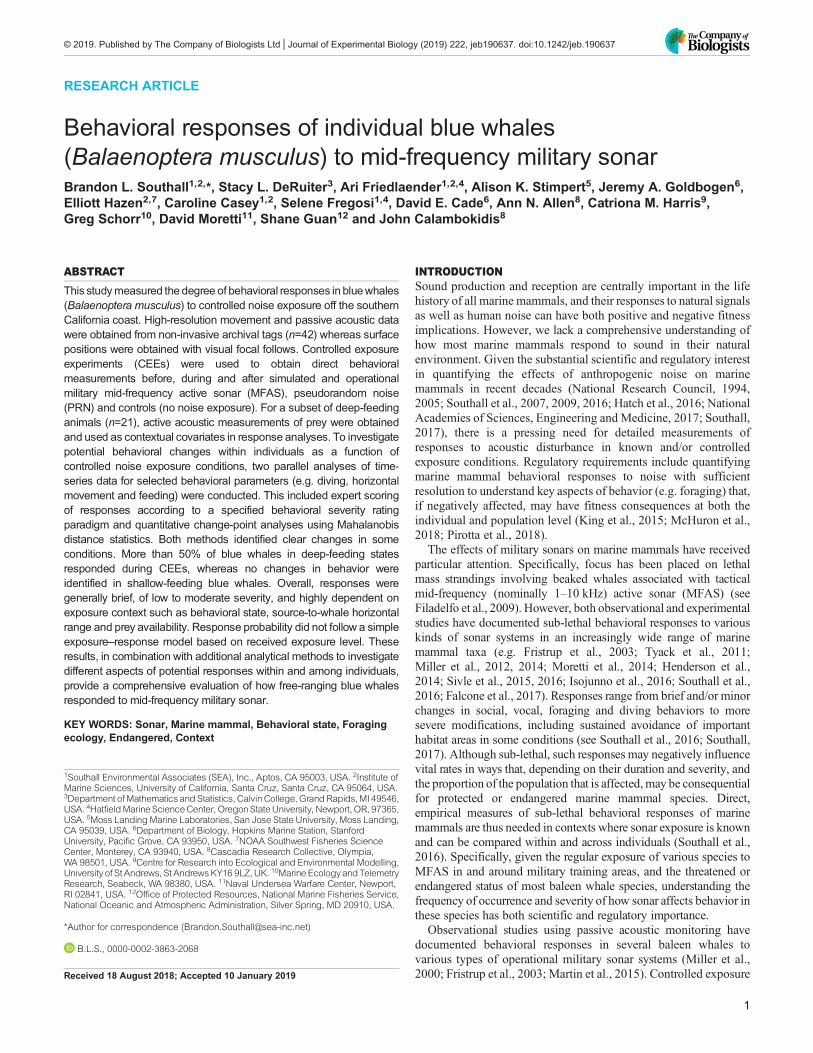
RESULTSCEEsA total of 48 CEE sequences were conducted for individual whalesinvolving MFAS, PRN or no-noise ‘control’ exposures in(primarily) coastal and offshore areas spanning the SouthernCalifornia Bight (Fig. 1). Data from six sequences in which tagsdetached prematurely or CEE sequences were terminated before15-min of exposure were not included in this analysis as they failedto meet specified experimental criteria; the remaining 42 sequencesmet these criteria and were analyzed. These occurred within 33discrete CEEs, as nine of these sequences involved two concurrentlytagged and followed animals. In seven of these instances,simultaneously tagged whales were separated from one anotherand were followed by separate boats. In two cases, simultaneouslytagged individuals occurred within close proximity and were beingtracked within the same focal follow, although one of these theanimals was later determined to be in different behavioral statesduring exposure. Four individual whales were later revealed throughphoto identification to have been exposed in two separate CEEswithin the same year. In each scenario, CEEs were spaced by severaldays or weeks. Furthermore, in each case, animals received differenttreatment types and were in different behavioral states for
CEE stimulusControl
Santa Barbara
N
Los Angeles
0 25 50 100km
34°0'N
33°0'N
117°0'W118°0'W119°0'W120°0'W
>–4000–2000–2000
MFASPRNReal MFAS
Depth (m)Fig. 1. Map of overall study area showing locations for allcontrolled exposure experiments (CEEs) conducted forall (n=42) blue whales. Treatment types for each CEE[control, simulated mid-frequency active sonar (MFAS),pseudo-random noise (PRN) and real MFAS] are indicated bydifferent symbols.
7
RESEARCH ARTICLE Journal of Experimental Biology (2019) 222, jeb190637. doi:10.1242/jeb.190637
1000 mN
N
N
34°33'N
–100
34°32'N
120°46'W
117°28'W 117°27'W
120°45'W
1000 m
–100
–200
–100
–500
120°44'W
118°18'W 118°17'W
33°12'N
33°11'N
33°10'N
33°41'N
33°40'N
33°39'N
Onset of exposure – 15:25 h
0
40
020
5.0
02.5
1.0
0
840
420
0.5
50
A B
C D
E F
180
160
140
120Dep
th (m
)
cSE
L(d
B re
.1 µ
Pa2
s)
Hea
ding
varia
nce
MD
15:10 15:25 15:40 15:55
180160140
cSE
L(d
B re
.1 µ
Pa2
s)
120100
16:10
17:24 17:39 17:54 18:09
17:29 17:44 17:59Local time (h)
18:14 18:29
100
150
0
40
020
5.0
02.5
1.0
0
6420
420
0.5
50100150200
0
50
Dep
th (m
)
100
150
4020
0
5.02.5
0
1.00.5
0
420
420
Lung
e ra
te(n
o. h
–1)
MS
A(m
s–2
)H
eadi
ngva
rianc
e
Hor
izon
tal
spee
d(m
s–1
)M
DOnset of exposure– 17:39 h
First pre-exposureposition – 15:01 h
End of post-exposureperiod – 16:19 h
First post-exposureposition – 16:02 h
First position followingexposure onset – 17:39 h
First pre-exposureposition – 17:18 h
End of post-exposureperiod – 18:30 h
First post-exposureposition – 18:03 h
Onset of exposure – 17:44 h
1000 m
–200
First position followingexposure onset – 17:51 h
First post-exposureposition – 18:16 h
End of post-exposureperiod – 18:38 h
First pre-exposureposition – 17:13 h
Focal followPre-exposureExposure
Exposure
km0 0.25 0.5 1 1.5
km0 0.25 0.5 1 1.5
km0 0.25 0.5 1 1.5
Post-exposureSource
Focal followPre-exposureExposure
Exposure
Post-exposureSource
Focal followPre-exposureExposure
Exposure
Post-exposureSource
First position followingexposure onset – 15:28 h
Dep
th (m
)Lu
nge
rate
(no.
h–1
) M
SA
(m s
–2)
Hea
ding
varia
nce
Hor
izon
tal
spee
d(m
s–1
)M
D
Hor
izon
tal
spee
d(m
s–1
)Lu
nge
rate
(no.
h–1
) M
SA
(m s
–2)
Fig. 2. See next page for legend.
8
RESEARCH ARTICLE Journal of Experimental Biology (2019) 222, jeb190637. doi:10.1242/jeb.190637
subsequent exposures. This likely reduced, but did not eliminate, thepotential that behavioral responses during the second CEEmay havebeen influenced to some degree by exposure to the initial CEE.The 42 discrete, randomized CEE sequences evaluated here were
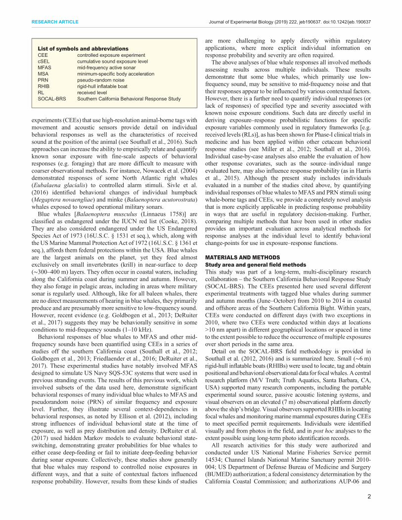
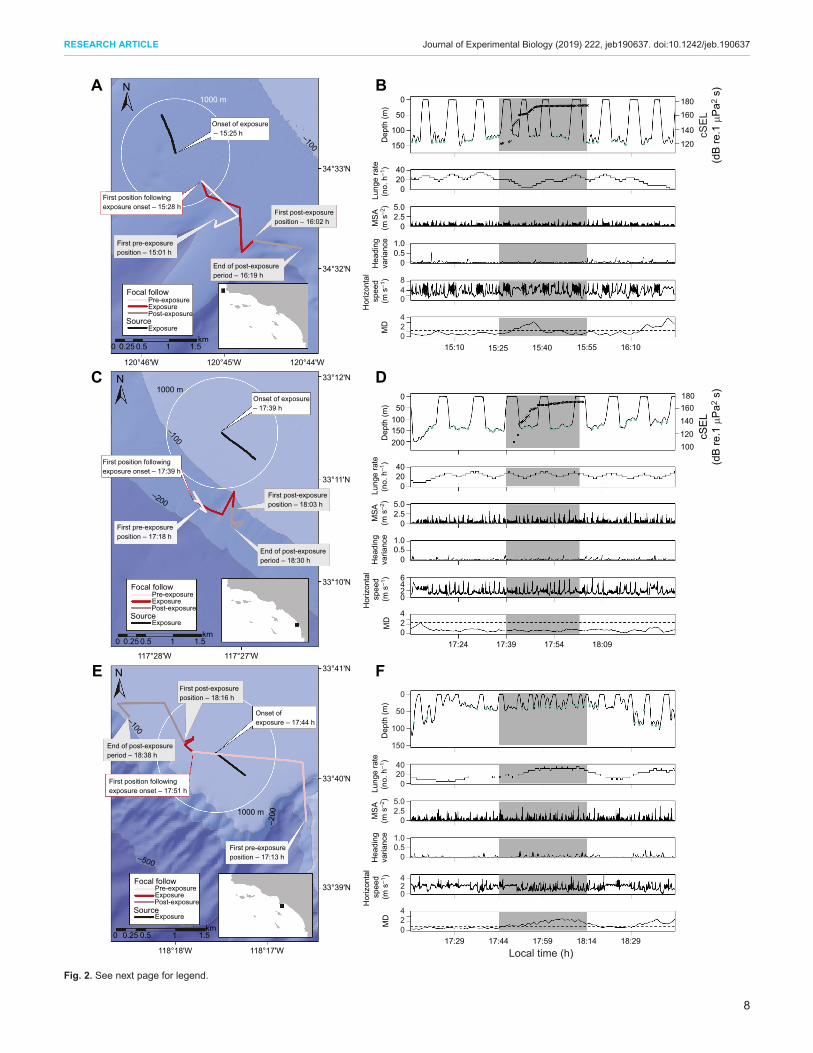
conducted during 2010–2014 field efforts within different exposuretreatments and behavioral state contexts. The resulting distributionof CEEs conducted for individuals within these three differentbehavioral states for each treatment type are summarized in Table 1.Representative examples of different types of behavioral responseresults for three individual whales are provided (Fig. 2).The results of CEE 2011-01 on 29 July 2011 with individual
bw11_210b are shown in time-annotated maps and MD data plotswith received cSEL (in dB re. 1 µPa2 s) in Fig. 2A,B. This was adeep-feeding blue whale exposed to MFAS at a source–whalehorizontal range (at the start of the exposure) of 1.2 km. Clearchanges in behavior were detected with both MD and expertscoring methods (high confidence scores) at virtually the sametime (15:28–15:29 h), corresponding to a received cSEL of119 dB re. 1 µPa2 s. Changes identified by adjudicated expertscoring included horizontal avoidance of sound source (severityscore 7) and moderate cessation of feeding (severity score 6) (seeTable S1 for expert scoring details). The results of CEE 2011-06 on6 August 2011 with individual bw11_218b are shown in Fig. 2C,D.This was a deep-feeding blue whale exposed to PRN at a source–whale range (at the start of the exposure) of 5.6 km. No changes inbehavior were detected with either MD or expert scoring methods(high confidence scores), despite a relatively high received cSEL of168 dB re. 1 µPa2 s (see Table S1 for expert scoring details). Theresults of CEE 2013-06 on 26 July 2013 with individual bw13_207aare shown in Fig. 2E,F. This was a shallow-feeding blue whalewithin a control sequence conducted at a source–whale range of0.5 km. No changes in behavior were detected with expert scoringmethods (moderate confidence scores), although the presence ofincreased feeding was noted (see Table S1 for expert scoringdetails). The increase in feeding rate resulted in a gradual increase inthe MD metric relative to the pre-exposure baseline condition andwas thus detected as a change. As in several other instances wherewhales initiated or increased feeding during CEEs, theMD-detectedchange was noted, but was not considered a conflicting result to theexpert scoring evaluation because an increase in feeding was notdefined as an adverse behavioral response (Southall et al., 2007;Miller et al., 2012).Expert scoring and MD results are presented for each treatment
type and behavioral state category for each individual blue whale(Table 2). Received exposure levels for each whale either atidentified change points or (where none were detected) maximumvalues for CEE sequences are also provided (Table 2). For CEEswith identified responses cSEL values at identified change pointsranged from 97 to 155 dB re. 1 µPa2 s. Maximum cSEL values for
CEEs where no change was identified ranged from 134 to171 dB re. 1 µPa2 s. Source–whale range varied from 0.4 to 7.7 kmfor the simulatedMFAS and 19.5 km for the single operational vesselMFAS signal, with a median range of 1.2 km. There was nosignificant correlation within experimental sound types (MFAS,PRN) across CEEs between RL and source–whale range.
Deep-feeding whalesThe largest number of individual CEE sequences analyzed (n=29)occurred for blue whales engaged in deep-feeding during pre-exposure periods.Whales were most likely to respond duringMFASCEE sequences, with a similar overall proportion of individualsidentified as changing behavior during exposure by both expertscoring (8 of 13) and MD (9 of 13) methods. A lower proportion ofdeep-feeding whales responded when exposed to PRN (4 of 11 inexpert scoring analysis; 5 of 11 for MD) and almost no responseswere detected in deep-feeding control sequences (0 of 5 for expertscoring; 1 of 5 for MD).
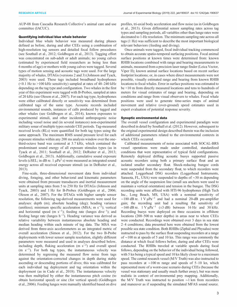
For a subset of deep-feeding whales (n=21), prey distribution anddensity were measured before and after CEE sequences to providean environmental context for interpreting responses in thisbehavioral state. Given the knowledge of the importance of thiscontextual relationship, we include three examples of whalebehavior and contextual prey data to illustrate how thesemeasurements provide additional insight into changes in whalebehavior and the interpretation of potential response (Fig. 3).
For bw11_210b on 29 July 2011 (Fig. 3A; Fig. S3), prey patchdepth and density remained similar both before and shortlyfollowing the CEE (2011-01) in the area where the whale wasfeeding. Both expert scoring groups identified very similarbehavioral changes with high confidence scores at approximatelythe same time as one another and similar to the MD analysis (seeTable S1 for expert scoring details), which identified a clear changerelative to not only the pre-exposure condition, but the entirebehavioral record for this individual (including pre-CEE preysampling periods). Given the similarity in the prey environmentbefore and at least immediately after the CEE, these identifiedchanges (avoidance and cessation of feeding) are unlikely the resultof changes in the prey environment (from the exposure orotherwise). However, subsequent changes in the overall preyenvironment (more schools identified at various depths) and/orchanges in the local prey environment based on the whale’sgeographic location may have also influenced whale behavior,particularly well after the CEE.
For bw11_218b on 6 August 2011 (Fig. 3B; Fig. S4), preypatches after the CEE (2011-06) were shallower than thosemeasured before the CEE sequence. This whale appeared toprogressively decrease its feeding depth and continue to feed duringthe CEE as it moved into an area with shallower patches. Thisgradual decrease in whale diving depth was not identified by eitherexpert-scoring group as a behavioral response during the CEE(Table S1). A behavioral change point was identified within theMDanalysis (see Fig. S4, where the MD trace crosses the dashed linerepresenting the pre-exposure baseline value used as the responsethreshold), although this was a small increase above the pre-exposure baseline period and it was of smaller magnitude than theMD spike in this metric identified just after the pre-CEE preysampling period.
For bw13_207a on 26 July 2013 (Fig. 3C; Fig. S5), prey patchesmeasured around the CEE (2013-06) in the areawhere the whale wasfeedingwere deeper and less dense following the CEE sequence thanbefore exposure. The animal maintained a similar feeding depth
Fig. 2. Movement, diving and feeding behavior for three CEEs duringpre-exposure (baseline), MFAS exposure and post-exposure phases.(A,C,E) Subject movement during each phase is shown in maps relativeto the sound source (sequential black circles showing the vessel’s drift) atexposure. (B,D,F) Whale diving behavior, showing: dive depth (m), lunges(green circles) and received cumulative sound exposure level (cSEL;dB re. 1 µPa2 s; right axis for panels B and D; black ‘x’), lunge rate (lunges h−1),maximum specific acceleration (MSA; m s–2), heading variance (unitless),calculated horizontal speed (m s–1) and Mahalanobis distance (MD) metrics(dashed line indicating maximum value in baseline conditions), with theexposure phase of CEEs shaded gray. Corresponding maps and plots areshown for: bw11_210b-CEE 2011-01 (A,B); bw11_218b-CEE 2011-06 (C,D);and bw13_207a-CEE 2013-06 (E,F).
9
RESEARCH ARTICLE Journal of Experimental Biology (2019) 222, jeb190637. doi:10.1242/jeb.190637
before and during the exposure sequence but increased its feedingrate and switched to deeper feeding after the CEE, which alsocontinued during the post-exposure prey sampling period. Neitherexpert scoring group identified any behavioral change in this CEE,but there was a discernible change detected using the MD method,associated with an increase in foraging during the exposure phaserelative to the defined baseline (pre-exposure) period (see Table S1for expert scoring details). These MD values were of similarmagnitude to those measured during both prey sampling periods(before and after the full CEE sequence).Cox proportional hazards models were fitted separately to
responses of severity scores between 4–6 and 7–9; responses with
severity scores of 1–3 were insufficient to apply this process. TheCox proportional hazards model selected by AIC for severity scores4–6 retained only source–whale range as a covariate (ΔAIC=1.34),although its effect was not significant (P=0.316). The selectedmodelmet the proportional hazards assumption (global P-value fromChi-square test=0.079). The model selected by AIC for severityscores 7–9 was the null model (ΔAIC=1.03), with the modelincluding source–whale range being the second best model accordingto AIC. Given the interest in understanding the role of source–whalerange in the probability of responding,model results from the selectedmodel for severity scores between 4 and 6 and the second-best modelfor severity scores between 7 and 9 were used to produce predicted
Table 2. Controlled exposure experiment (CEE) results for all blue whales in deep-feeding, shallow-feeding and non-feeding behavioral states
Subjectbehavioral stateand CEE type Subject ID
Source–whalerange (km)
Max.cSEL(dB re.1 µPa2 s)
Behavioral change identified?
Methodsagree?
Total MDchanges‡
Total ESchanges
Mahalanobis distance (MD) Expert scoring (ES)
Changeidentified?
Received cSELat change point(dB re. 1 µPa2 s)
Change?(confidencescore)
Scoredseverity
Received cSELat change point(dB re. 1 µPa2 s)
Deep-feedingcontrol (n=5)
bw10_241a 0.3 n/a No n/a No (high) 0 n/a Yes 1 of 5 0 of 5bw10_241_B034 1.75 n/a No n/a No (low) 0 n/a Yesbw14_212a 1.3 n/a Yes n/a No (low) 0 n/a Nobw14_213a 0.7 n/a No n/a No (low) 0 n/a Yesbw14_251a 1.25 n/a Yes* n/a No (high) 0 n/a Yes
bw10_243a 4.6 157 No – No (high) 0 – Yes 5 of 11 4 of 11bw10_243b 0.8 160 Yes* – No (low) 0 – Yesbw10_244b 1.15 168 Yes 105 No (moderate) 0 – Nobw10_244c 1.6 160 Yes 158 Yes (high) 7 110 Yesbw10_245a 7.7 149 Yes* – No (high) 0 – Yesbw10_266a 1.25 160 Yes 148 Yes (high) 7 148 Yesbw11_211a 1.1 162 No – No (high) 0 – Yesbw11_214b 0.4 160 Yes 109 Yes (high) 6 109 Yesbw11_218b 1.2 168 No – No (high) 0 – Yesbw11_221a 0.6 160 Yes 124 Yes (low) 5 97 Yesbw11_221b 0.6 162 No – No (low) 0 – Yes
Shallow-feedingcontrol (n=1)
bw13_207a 0.5 n/a Yes* n/a No (moderate) 0 n/a Yes 0 of 1 0 of 1
Shallow-feedingMFAS (n=7)
bw10_235a 1.05 170 No – No (low) 0 – Yes 0 of 7 0 of 7bw10_235b 1.7 145 Yes* – No (moderate) 0 – Yesbw10_238a 0.45 152 No – No (moderate) 0 – Yesbw10_240a 0.5 169 Yes* – No (high) 0 – Yesbw10_240b 3.7 165 No – No (high) 0 – Yesbw13_259a 5.2 134 No – No (moderate) 0 – Yesbw14_262a 1.4 142 Yes* – No (moderate) 0 – Yes
Non-feedingMFAS (n=2)
bw10_235_B019 1.9 158 Yes 108 Yes (high) 7 108 Yes 2 of 2 1 of 2bw10_265a 1.9 158 Yes 148 No (moderate) 0 – No
Non-feedingPRN (n=3)
bw10_251a 0.85 159 Yes 123 Yes (low) 7 102 Yes 3 of 3 1 of 3bw11_218a 5.6 137 Yes 102 No (moderate) 0 – Nobw12_292a 1.15 157 Yes 127 No (high) 0 – No
*Associated with onset of feeding in MD change-point; this was not scored as a response within ES.‡Not including identified MD changes associated with feeding onset.Maximum received cumulative sound exposure levels (cSEL; dB re. 1 µPa2 s) are given for all individuals for all CEEs involving noise exposure. Behavioral changes identified usingwith Mahalanobis distance statistical change-point methods and ES are presented for each whale and summarized within each behavioral state and CEE treatment type. Relativeconfidence scores (low, moderate, high) for ES panels as well as the highest attributed response severity are provided.Where behavioral changeswere detected, received cSEL is given atchange points identified by MD and ES methods. Whether analytical methods agree in detecting changes is identified and total changes for MD analyses (excluding instances wherechanges were associated with feeding onset) and ES results are compared within categories.
10
RESEARCH ARTICLE Journal of Experimental Biology (2019) 222, jeb190637. doi:10.1242/jeb.190637
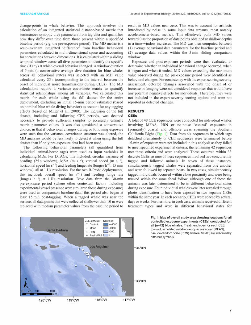
exposure–response probability functions in terms of receivedexposure level for the two different response severity levels(moderate severity: 4–6; high severity: 7–9). In order to illustratethe relationship with source–animal range, response probabilityfunctions were calculated for the ranges over which most CEEs wereconducted (1–5 km) (Fig. 4). These prediction plots suggest that theprobability of a moderate response (severity 4–6) as a function of RLdecreases rapidly as range increases, but thewide confidence intervalsindicate substantial uncertainty in this relationship. The relationship ismuch less pronounced for high severity responses (severity 7–9),hence the selection of the null model.
Shallow-feeding and non-feeding whalesThe second largest number of individual CEE sequences analyzed(n=8) occurred for blue whales engaged in shallow feeding duringpre-exposure periods. Nowhales (0 of 7) were determined to changebehavior during MFAS exposure by either expert scoring or MDmethods. No PRN sequences were conducted for shallow-feedingwhales. No responses were detected by either analytical methodduring the single shallow-feeding control sequence.
The fewest number of individual CEE sequences analyzed (n=5)occurred for non-feeding blue whales, although most of theseindividuals were determined to have an adverse behavioral responseduring CEEs across both methods. For MFAS CEE sequences, expertscoring determined such a response in one of two whales, whereasMD analyses detected adverse responses for both individuals. ForPRNCEEs, expert scoring determined an adverse behavioral responsein one of three non-feeding whales, whereas all three individuals wereidentified to have such a response using MD methods. No controlsequences were conducted for non-feeding whales.
Vessel noise characterizationMedian values of vessel noise were calculated for the closest pointof approach for all vessels during each condition. These values werecompared for each condition for the RHIBs Ziphid and Physaluswith comparable measurements of ambient noise made using thesame recorders and methods during the same day and similarconditions, with these vessels operating at much further ranges fromrecording buoys (Fig. S1). Ambient noise measurements were alsocompared for each passage condition for the M/V Truth withcomparable measurements of ambient noise made using the samerecorders and methods during the same day and similar conditions,with this vessel operating at much further ranges from recordingbuoys (Fig. S2A,B). For the stationary M/V Truth maneuvering at∼1 km range from recorders, median noise values were calculatedrelative to ambient noise during the same day and similar conditions(Fig. S2C). Both RHIBs and the M/V Truth were clearly detectableover ambient noise for both speeds at these close ranges, withdifferent relative spectral distribution of noise energy at differentspeeds for each vessel. Based on the associated noise levels andfrequencies and typical ambient noise during non-vessel periods,their operation is likely audible to subjects over ranges typicalduring CEEs, particularly the RHIBs at their typical operatingspeeds and ranges from animals. However, as a part of theexperimental design during the pre-exposure (baseline), exposureand post-exposure sequences, these represent relatively continuouslevels of additional noise exposure. During sound sourcedeployment, the M/V Truth conducted small maneuvers to remainstationary. The measurements of ambient noise during this perioddemonstrated that these maneuvers and the presence of the vesselwere not discriminable over noise measured using the samerecording system in the absence of the M/V Truth. That is,
0
A
B
C
50
100
150
200
Dep
th (m
)M
DD
epth
(m)
MD
Dep
th (m
)M
D
250
–42–44–46–48–50–52–54
–50–52–54–56–58–60–62–64
–50
–55
–60
43210
0
50
100
150
200
16:41 18:41 20:41
11:27 13:27 15:27 17:27
15:56 16:56 17:56 18:56Local time (h)
43210
050
100150200250300350
43210
dB
dB
dB
Fig. 3. Movement, diving and feeding behavior for three CEEs for whichblue whale prey (krill) schools were measured using active acousticsbefore and after experimental sequences. Longitudinal plots showindividual whale dive profiles (top) and MD plots (bottom) with the exposurephase of CEEs shaded gray. Feeding lunges are marked as green circlesand prey patches measured in close horizontal proximity to feeding whalesare shown at their respective depth (m) in relative patch density (dB)expressed as relative size and color (denser patches are larger and redder).Corresponding dive profiles and MD plots are shown for: bw11_210b-CEE2011-01 (A); bw11_218b-CEE 2011-06 (B); and bw13_207a-CEE2013-06 (C).
11
RESEARCH ARTICLE Journal of Experimental Biology (2019) 222, jeb190637. doi:10.1242/jeb.190637
although vessels were likely audible during their operation,particularly during pre- and post-exposure periods, when the M/VTruth was following focal animals, during exposure periods, noisefrom the sound source vessel received by experimental subjects waspredominately or exclusively the result of experimental exposures.
DISCUSSIONThis study generated the largest sample size (n=42) for anyexperimental behavioral response study involving sonar conductedto date for any marine mammal species (Southall et al., 2016).Although the number of individual CEEs conducted in somebehavioral states and treatments were limited, dozens of controlledindividual experiments were conducted using high-resolutionmovement and acoustic sensors for individuals in well-definedexposure contexts. These results provide direct and robust means ofevaluating how an endangered species responds to noise exposure,including simulated and actual militaryMFAS signals that have beenassociated with lethal responses in other species. The analyticalapproach provides a direct means of quantifying individual behaviorand behavioral responses within known noise exposure conditionsin such a way that probabilistic response functions may be generatedin light of important contextual variables. Such data providean empirical basis for modeling efforts to evaluate potentialconsequences of disturbance at broader population scales (Kinget al., 2015; McHuron et al., 2018; Pirotta et al., 2018).Blue whales responded to noise in some but not all CEE
sequences (19 of 37 for MD analysis; 14 of 37 for expert scoring)and in almost no control (no-noise) sequences (1 of 6 for MDanalysis; 0 of 6 for expert scoring). Treatment types had variablesample sizes, but responses were generally equally likely to occurforMFAS and PRN exposures. Other than a single instance detectedonly with the MD method, none occurred during control (no noise)sequences. Nine CEEs involved exposure of multiple individuals,
although nearly all of these included animals in separate groups. Asmall number of CEEs involved paired individuals or subsequentexposures to the same individuals and in two instances in the firstyear of the study animals could have been remotely exposed toan earlier CEE prior to being the focal animal in a subsequentCEE later in the day. Although these could call into questionthe treatment of all individuals as independent samples, they weretreated as such here (rather than excluding individuals) given thesmall number of instances relative to the overall sample size.Further, we took into consideration the fact that in all but oneinstance these CEEs all involved differences in individualbehavioral state and/or treatment type.
Responses generally included short-term changes in divingbehavior, small-scale (a few kilometers) horizontal avoidance ofsound source location and/or cessation of feeding activity. Recoveryto typical pre-exposure behavior in most CEEs typically occurredwithin the post-exposure phase. However, the short-term andrelatively rapid nature of recovery should be considered within thecontext of acknowledged differences between the MFAS from anexperimental source and operational MFAS. The experimentalMFAS is stationary, includes a ramp-up escalation of the sourcelevel, and the overall duration is relatively short (tens of minutes).Operational MFAS training involves much louder and constantlevels and can occur over many hours or even days in the case ofmulti-ship operations (see Moretti et al., 2014). It can also occurat any hour of the day and throughout the year, whereas CEEshere were only conducted during daylight hours in the summerand autumn.
Two different analytical approaches were applied to evaluatebehavioral changes from baseline conditions within individualsusing high-resolution, time-series kinematic and acoustic data. Thisapproach included both quantitative statistical change-point methodsand structured expert scoring assessment of deviations from baseline
0.6
1 km 2 km 5 km
0.4
0.2
0
0.6
0.4
0.2
0
110 130 150 170 110 130cSEL
(dB re. 1 µPa2 s)
Pro
babi
lity
of re
spon
se
Sev
erity
sco
re 4
–6S
ever
ity s
core
7–9
150 170 110 130 150 170
Fig. 4. Behavioral response probability for deep-feeding blue whales exposed to MFAS and PRNas a function of received cSEL (dB re. 1 µPa2 s)for different source–receiver ranges and expertscored response severities. Response probabilitymodel predictions (black lines) with 95% confidencelimits (shaded gray areas) are shown for 1, 2 and 5 kmsource–receiver ranges for moderate (scores 4–6) andhigh response severity (scores 7–9).
12
RESEARCH ARTICLE Journal of Experimental Biology (2019) 222, jeb190637. doi:10.1242/jeb.190637
conditions during exposure by subject matter experts. The MDmethod is inherently objective in that it simply identifies changes in asuite of variables from baseline (pre-exposure) conditions and is thusequally likely to detect a behavioral change associated with apresumably positive outcome (e.g. an increase in foraging behavior)as a presumably negative outcome (cessation of feeding). Further, theselection of a response ‘threshold’ for MD strongly affects theprobability of statistically detecting a behavioral response. Here, afairly low MD value was selected as a change-point threshold,namely, an MD value within the exposure period exceeding thatmeasured during the pre-exposure period. This results in a higherlikelihood of identifying a behavioral response than if an alternatethreshold were selected (e.g. two standard deviations exceeding thepre-exposure maximum) or if MD values during exposure exceededthe pre-exposure maximum value across the entire tag record.However, the intent here was to identify a discernible change inbehavior during an exposure period with a similar context as pre-exposure conditions (e.g. local environmental variables, proximity ofvessels) rather than aiming to identify a change that was more unusualthan any other change measured for that or any other blue whale. Notsurprisingly, the MDmethod was more likely to detect a change thanexpert scoring, both in controls and exposures. However, oncedetected changes associated with the onset of feeding (presumablynot an adverse behavioral change) were discounted, results were quitesimilar across individuals. Some differences were still observed, butfor 32 of 42CEEs (76%), themethods agreed as towhether an adversebehavioral change occurred (where changes associated with the onsetof feeding were excluded). Further, detected changes tended to occurat similar exposure times and associated RLs. Expert scoring methodswere consequently consistent with the MD method in identifyingbehavioral changes, but this approach also has the advantage of beingdescriptive and identifying changes associated with various types ofbehavior (movement, feeding), including variability in responseseverity and the level of confidence in discerning response bothwithin and between groups. Although both methods have advantagesand limitations, the general agreement here was encouraging, andhaving used both methods provides more comprehensive insight intochanges during experimental exposures. Future studies shouldconsider integrating objective statistical change-point analyses (e.g.MD results) within expert evaluation of potential responses.These findings demonstrate the kinds of context-specific
differences in behavioral response identified by Ellison et al.(2012). Along these lines, they also complement and expand uponthe findings of Goldbogen et al. (2013) and DeRuiter et al. (2017)regarding the importance of behavioral state in terms of responseprobability for blue whales, specifically the increased likelihoodof response in deep-feeding animals. This study provides adifferent perspective on this behavioral state dependency inevaluating individual response type and severity for knownexposure conditions for a relatively large sample size. Given theseobservations, we note the contextual differences between thesimulated MFAS and some kinds of operational MFAS sourcessuch as the SQS-53C sonar used in one CEE here; there are greatercontextual similarities between the experimental source and othercommon operational military MFAS sources such as helicopter-dipping sonars. The experimental MFAS has proven useful indemonstrating previously unknown aspects of behavior, responseand context dependency in these species, but, as we have shown,differences in exposure parameters can influence responseprobability. Additional research, some of which has beenconducted and some of which is underway, is needed to furtherevaluate the importance of contextual differences in sound source
type (e.g. source level, movement, spectral features) and proximity.This approach with individual animals where exposure range wasknown allowed for a quantification of behavioral response probabilityas a function of proximity to the sound source (Fig. 4) for the rangestested. Deep-feeding whales had a higher response probability whenlocated closer to the sound source for comparable RLs, although thereis considerable uncertainty within the relationships and insufficientdata to test this relationship for other behavioral states. Given theavailable data at this point, a simple relationship between sourcerange, RL and response probability across all whales does not appearto exist. Further evaluation of the potential range-dependenceidentified within this study using a dedicated experimental designto test and further resolve these seemingly important range–RLrelationships is needed before firm conclusions can be drawn.Specifically, additional studies should explicitly evaluate differentdimensions of the RL–range space, including potential changesduring near but quieter exposure conditions.
Whale dive depth has been closely linked to changes in preypatch depth, thus prey can both mediate the response to sonarplaybacks when prey are dense and confound potential responseswhen prey distributions are not known. Although a directquantitative comparison is not possible for all individuals, giventhe absence of before and after prey data in some cases, our resultswere consistent with Friedlaender et al. (2016) in suggesting that thebehavior of feeding blue whales is broadly influenced by features ofthe prey environment in ways that likely mediate responses to CEEs.Specifically, two of the three instances where the MD detected CEEresponses were potentially a result of changes in prey while expertscoring classified 0 of the 3 as a CEE response (see Table S1 foradditional details). This highlights a potential strength in expertscoring in identifying specific aspects of a response in the absenceof known important contextual variables. Changes in prey patchdepth have been shown to result in commensurate changes in whaledive depth, and for some individuals, the likelihood of a behavioralresponse to navy sonar during a playback is reduced with increasedprey density while foraging.
Many regulatory efforts to evaluate the effects of noise on marinemammals have primarily or exclusively used received noiseexposure level as a predictor of response probability and havesought to develop more robust predictive associations. As illustratedby Ellison et al. (2012), a host of contextual factors can influencebehavioral responses to noise. Several key contextual influenceswere identified here (and see Goldbogen et al., 2013; Friedlaenderet al., 2016; DeRuiter et al., 2017) that have strong effects onwhetherand how endangered blue whales respond when exposed to militaryMFAS signals or PRN of similar frequency and duration. Responseswere mediated by a complex interaction of the animal’s behavioralstate at the time of exposure, features of the environment and therelative proximity of sound sources. Without identifying behavioralstate using objective, quantitative metrics (e.g. dive depth, presenceof foraging lunges) and considering this as a relevant contextualvariable, it would have been much more difficult to unravel thecomplexity of these relationships across studies. Identifying this,within certain contexts, indicates that an increase in RLs is in factassociated with an increase in response probability. Although thiscomplexity is not yet fully understood, relating response probability,exposure level and behavioral state dependency will enable a moreinsightful and informed understanding of exposure–responserelationships. This does not mean that each behavioral state and/orprey contextual conditionmust be informed by distinct and empiricalexposure–response risk functions for management applications.Rather, integrated risk functions within behavioral states
13
RESEARCH ARTICLE Journal of Experimental Biology (2019) 222, jeb190637. doi:10.1242/jeb.190637
(e.g. foraging, traveling) and a small subset of contextual covariates(e.g. range) might be informed by targeted experimental studies insome species where relatively large sample sizes may be obtained(see Southall et al., 2016; Southall, 2017).These results provide further evidence and increased resolution
on how baleen whales respond to noise exposure. They also providemuch-needed direct measurements of behavioral responses in anendangered species commonly exposed to MFAS within importanthabitat areas off California. As has been noted in other studies (seeSouthall et al., 2016; Southall, 2017), results from locations wheresonar exposure is common are likely much different from thebehavioral responses of animals from areas where sonar exposure isuncommon or absent. Although blue whales are likely low-frequency specialists, they can and do respond to soundspresented to them with primary energy in the 3–4 kHz rangeassociated with many MFAS systems found in commercial, navaland recreational platforms.Whales that do respond appear to recoverto typical behavioral patterns relatively quickly based on the resultsfrom these CEEs, and their probability of response should beconsidered given the contextual dependencies described in thisstudy.With increased energetic demands and needs for high-densityprey, even the cessation of feeding for a short time could haveconsequences for the fitness of these large animals (see Goldbogenet al., 2013). If they are chronic, they could manifest as population-level effects. Future experimental studies and targeted monitoringinformed by these results should focus on the energetic and, in turn,biological consequences of behavioral responses across differentbehavioral states.
AcknowledgementsThis 5-year study represented a major portion of the overall SOCAL-BRS projectand could not have been conducted without the tireless support of many dedicatedfield personnel. We sincerely appreciate the Truth Aquatics team for their sustainedinvolvement and support. We would also like to specifically acknowledge thecontributions of: Kristin Southall, Peter Tyack, Jay Barlow, Shannon Rankin,Fleur Visser, Annie Douglas, Erin Falcone, Katy Laveck, Jeff Foster, Todd Pusser,Glenn Gailey, Doug Nowacek, Louise Burt, John Hildebrand, Ron Morrissey,Greg Juselis, Jolie Harrison, Tami Adams, Sarah Wilkin, Ned Cyr, Frank Stone,Bob Gisiner and Mike Weise. We also thank two anonymous reviewers, whogreatly improved the quality of the manuscript.
Competing interestsThe authors declare no competing or financial interests.
FundingPrimary funding for the SOCAL-BRS project was initially provided by the U.S.Navy’s Chief of Naval Operations Environmental Readiness Division andsubsequently by the U.S. Navy’s Living Marine Resources Program. Additionalsupport for environmental sampling and logistics was also provided by the Officeof Naval Research, Marine Mammal Program. Additional support to enableS. Guan’s participation was provided by the U.S. National Oceanic andAtmospheric Administration.
Data availabilityThe complete dataset of all expert scoring and statistical analysis plots andindividual results for all 42 whales is also available online via Dryad (Southall et al.,2019; http://dx.doi.org/10.5061/dryad.d0mv3dh).
Supplementary informationSupplementary information available online athttp://jeb.biologists.org/lookup/doi/10.1242/jeb.190637.supplemental
ReferencesCade, D. E., Barr, K. R., Calambokidis, J., Friedlaender, A. S. and Goldbogen,
J. A. (2018). Determining forward speed from accelerometer jiggle in aquaticenvironments. J. Exp. Biol. 221, jeb170449.
Cooke, J. G. (2018). Balaenoptera musculus. The IUCN Red List of ThreatenedSpecies 2018: e.T2477A50226195.
DeRuiter, S. L., Southall, B. L., Calambokidis, J., Zimmer, W. M. X., Sadykova,D., Falcone, E. A., Friedlaender, A. S., Joseph, J. E., Moretti, D., Schorr, G. S.et al. (2013). First direct measurements of behavioural responses by cuvier ‘sbeaked whales to mid-frequency active sonar. Biol. Lett. 9, 20130223.
DeRuiter, S. L., Langrock, R., Skirbutas, T., Goldbogen, J. A., Calambokidis, J.,Friedlaender, A. S. and Southall, B. L. (2017). A multivariate mixed hiddenMarkov model for blue whale behaviour and responses to sound exposure. Ann.Appl. Stat. 11, 362-392.
Ellison, W. T., Southall, B. L., Clark, C. W. and Frankel, A. S. (2012). A newcontext-based approach to assess marine mammal behavioral responses toanthropogenic sound. Conserv. Biol. 26, 21-28.
Falcone, E. A., Schorr, G. S., Watwood, S. L., DeRuiter, S. L., Zerbini, A. N.,Andrews, R. D., Morrissey, R. P. and Moretti, D. J. (2017). Diving behaviour ofCuvier’s beaked whales exposed to two types of military sonar. R. Soc. Open Sci.4, 170629.
Filadelfo, R., Mintz, J., Michlovich, E., D’Amico, A., Tyack, P. L. and Ketten,D. R. (2009). Correlating military sonar use with beaked whale mass strandings:What do the historical data show? Aquat. Mamm. 35, 435-444.
Friedlaender, A. S., Goldbogen, J. A., Nowacek, D. P., Read, A. J., Johnston, D.and Gales, N. (2014). Feeding rates and under-ice foraging strategies of thesmallest lunge filter feeder, the Antarctic minke whale (Balaenopterabonaerensis). J. Exp. Biol. 217, 2851-2854.
Friedlaender, A. S., Hazen, E. L., Goldbogen, J. A., Stimpert, A. K.,Calambokidis, J. and Southall, B. L. (2016). Prey-mediated behavioralresponses of feeding blue whales in controlled sound exposure experiments.Ecol. Appl. 26, 1075-1085.
Fristrup, K. M., Hatch, L. T. and Clark, C. W. (2003). Variation in humpback whale(Megaptera novaeangliae) song length in relation to low-frequency soundbroadcasts. J. Acoust. Soc. Am. 113, 3411-3424.
Goldbogen, J. A., Calambokidis, J., Shadwick, R. E., Oleson, E. M., McDonald,M. A. and Hildebrand, J. A. (2006). Kinematics of foraging dives and lunge-feeding in fin whales. J. Exp. Biol. 209, 1231-1244.
Goldbogen, J. A., Southall, B. L., DeRuiter, S. L., Calambokidis, J.,Friedlaender, A. S., Hazen, E. L., Falcone, E. A., Schorr, G. S., Douglas, A.,Moretti, D. J. et al. (2013). Blue whales respond to simulated mid-frequencymilitary sonar. Proc. R. Soc. B 280, 20130657.
Goldbogen, J. A., Stimpert, A. K., DeRuiter, S. L., Calambokidis, J.,Friedlaender, A. S., Schorr, G. S., Moretti, D. J., Tyack, P. L. and Southall,B. L. (2014). Using accelerometers to determine the calling behavior of taggedbaleen whales. J. Exp. Biol. 14, 2449-2455.
Harris, C. M., Sadykova, D., DeRuiter, S. L., Tyack, P. L., Miller, P. J. O.,Kvadsheim, P. H., Lam, F. P. A. and Thomas, L. (2015). Dose response severityfunctions for acoustic disturbance in cetaceans using recurrent event survivalanalysis. Ecosphere 6, 1-14.
Hatch, L. T., Wahle, C. M., Gedamke, J., Harrison, J., Laws, B., Moore, S. E.,Stadler, J. H. and Van Parijs, S. E. (2016). Can you hear me here? Managingacoustic habitat in us waters. Endanger. Species Res. 30, 171-186.
Hazen, E. L., Friedlaender, A. S. and Goldbogen, J. A. (2015). Blue whales(Balaenoptera musculus) optimize foraging efficiency by balancing oxygen useand energy gain as a function of prey density. Sci. Adv. 1, e1500469-e1500469.
Henderson, E. E., Smith, M. H., Gassmann, M., Wiggins, S. M., Douglas, A. B.and Hildebrand, J. A. (2014). Delphinid behavioral responses to incidental mid-frequency active sonar. J. Acoust. Soc. Am. 136, 2003-2014.
Isojunno, S., Cure, C., Kvadsheim, P. H., Lam, F. P. A., Tyack, P. L., Wensveen,P. J. and Miller, P. J. O. (2016). Sperm whales reduce foraging effort duringexposure to 1–2 kHz sonar and killer whale sounds. Ecol. Appl. 26, 77-P. 93.
Johnson, M. P. and Tyack, P. L. (2003). A digital acoustic recording tag formeasuring the response of wild marine mammals to sound. IEEE J. Oceanic Eng.28, 3-12.
King, S. L., Schick, R. S., Donovan, C., Booth, C. G., Burgman, M., Thomas, L.and Harwood, J. (2015). An interim framework for assessing the populationconsequences of disturbance. Methods Ecol. Evol. 6, 1150-1158.
Kleinbaum, D. G. and Klein, M. (2010). Competing risks survival analysis. InSurvival Analysis: A Self-Learning Text, pp. 425-495. New York: Springer.
Mahalanobis, P. C. (1936). On the generalized distance in statistics. Proc. Nat. Inst.Sci. India 2, 49-55.
Martin, S. W., Martin, C. R., Matsuyama, B. M. and Henderson, E. E. (2015).Minke whales (Balaenoptera acutorostrata) respond to navy training. J. Acoust.Soc. Am. 137, 2533-2541.
14
RESEARCH ARTICLE Journal of Experimental Biology (2019) 222, jeb190637. doi:10.1242/jeb.190637
McHuron, E. A., Schwarz, L. K., Costa, D. P. and Mangel, M. (2018). A state-dependent model for assessing the population consequences of disturbance onincome-breeding mammals. Ecol. Model. 385, 133-144.
Miller, P. J. O., Biassoni, N., Samuels, A. and Tyack, P. L. (2000). Whale songslengthen in response to sonar. Nature 405, 903.
Miller, P. J. O., Johnson, M. P., Madsen, P. T., Biassoni, N., Quero, M. and Tyack,P. L. (2009). Using at-sea experiments to study the effects of airguns on theforaging behavior of sperm whales in the Gulf of Mexico. Deep Sea Res. Part IOceanogr. Res. Pap. 56, 1168-1181.
Miller, P. J. O., Kvadsheim, P. H., Lam, F. P. A., Wensveen, P. J., Antunes, R.,Alves, A. C., Visser, F., Kleivane, L., Tyack, P. L. and Sivle, L. D. (2012). Theseverity of behavioral changes observed during experimental exposures of killer(Orcinus orca), long-finned pilot (Globicephala melas), and sperm (Physetermacrocephalus) whales to naval sonar. Aquat. Mamm. 38, 362-401.
Miller, P. J. O., Antunes, R. N., Wensveen, P. J., Samarra, F. I. P., Alves, A. C.,Tyack, P. L., Kvadsheim, P. H., Kleivane, L., Lam, F.-P. A., Ainslie, M. A. et al.(2014). Dose-response relationships for the onset of avoidance of sonar by free-ranging killer whales. J. Acoust. Soc. Am. 135, 975-993.
Moretti, D., Thomas, L., Marques, T., Harwood, J., Dilley, A., Neales, B., Shaffer,J., McCarthy, E., New, L., Jarvis, S. et al. (2014). A risk function for behavioraldisruption of Blainville’s beaked whales (Mesoplodon densirostris) from mid-frequency active sonar. PLoS ONE 9, e85064.
National Research Council (1994). Low-Frequency Sound in Marine Mammals:Current Knowledge and Research Needs. Washington, DC: The NationalAcademies Press.
National Research Council (2005).Marine Mammal Population and Ocean Noise:Determining when Noise Causes Biologically Significant Effects. Washington,DC: The National Academies Press.
National Academies of Sciences, Engineering and Medicine (2017).Approaches to Understanding Cumulative Effects of Stressors of MarineMammal. Washington, DC: The National Academies Press.
Nowacek, D. P., Johnson, M. P. and Tyack, P. L. (2004). North Atlantic right whales(Eubalaena glacialis) ignore ships but respond to alerting stimuli. Proc. R. Soc.Lond. B 271, 227-231.
Oleson, E. M., Calambokidis, J., Burgess, W. C., McDonald, M. A., LeDuc, C. A.and Hildebrand, J. A. (2007). Behavioral context of call production by easternNorth Pacific blue whales. Mar. Ecol. Prog. Ser. 330, 269-284.
Pirotta, E., Mangel, M., Costa, D. P., Mate, B., Goldbogen, J. A., Palacios, D. M.,Huckstadt, L. A., McHuron, E. A., Schwarz, L. and New, L. (2018). A dynamicstate model of migratory behavior and physiology to assess the consequences of
environmental variation and anthropogenic disturbance on marine vertebrates.Am. Nat. 191, E40-E56.
Simon, M., Johnson, M. and Madsen, P. T. (2012). Keeping momentum with amouthful of water: behavior and kinematics of humpback whale lunge feeding.J. Exp. Biol. 215, 3786-3798.
Sivle, L. D., Kvadsheim, P. H., Cure, C., Isojunno, S., Wensveen, P. J., Lam, F.-P.A., Visser, F., Kleivanec, L., Tyack, P. L., Harris, C. M. et al. (2015). Severity ofexpert-identified behavioural responses of humpback whale, minke whale, andnorthern bottlenose whale to naval sonar. Aquat. Mamm. 41, 469-502.
Sivle, L. D., Wensveen, P. J., Kvadsheim, P. H., Lam, F. P. A., Visser, F., Cure, C.,Harris, C. M., Tyack, P. L. and Miller, P. J. O. (2016). Naval sonar disruptsforaging in humpback whales. Mar. Ecol. Prog. Ser. 562, 211-220.
Southall, B. L. (2017). Noise. In Encyclopedia of Marine Mammals, 3rd edn (ed. B.Wursig and H. Thiewesson), pp. 699-707. New York: Academic Press.
Southall, B. L., Bowles, A. E., Ellison, W. T., Finneran, J. J., Gentry, R. L.,Greene, C. R., Kastak, D., Ketten, D. R., Miller, J. H., Nachtigall, P. E. (2007).Marine mammal noise exposure criteria. Aquat. Mamm. 33, 411-521.
Southall, B. L., Bowles, A. E., Ellison, W. T., Finneran, J. J., Gentry, R. L.,Greene, C. R., Kastak, D., Ketten, D. R., Miller, J. H., Nachtigall, P. E. et al.(2009). Marine mammal noise exposure criteria: initial scientificrecommendations. J. Acoust. Soc. Am. 125, 2517-2517.
Southall, B. L., Moretti, D., Abraham, B., Calambokidis, J., DeRuiter, S. L. andTyack, P. L. (2012). Marine mammal behavioral response studies in southernCalifornia: advances in technology and experimental methods. Mar. Technol.Soc. J. 46, 48-59.
Southall, B. L., Nowacek, D. P., Miller, P. J. O. and Tyack, P. L. (2016).Experimental field studies to measure behavioral responses of cetaceans tosonar. Endanger. Species Res. 31, 293-315.
Southall, B. L., DeRuiter, S. L., Friedlaender, A., Stimpert, A. K., Goldbogen,J. A., Hazen, E., Casey, C., Fregosi, S., Cade, D. E., Allen, A. N. et al. (2019).Data from: Behavioral responses of individual blue whales (Balaenopteramusculus) to mid-frequency military sonar. Dryad Digital Repository. http://dx.doi.org/10.5061/dryad.d0mv3dh
Therneau, T. M. and Grambsch, P. M. (2000). Multiple events per subject. InModeling Survival Data: Extending the Cox Model, pp. 169-230. New York:Springer.
Tyack, P. L., Zimmer, W. M., Moretti, D., Southall, B. L., Claridge, D. E., Durban,J. W., Clark, C. W., D’Amico, A., DiMarzio, N., Jarvis, S. et al. (2011). Beakedwhales respond to simulated and actual navy sonar. PloS ONE, 6, e17009.
Highlighted Article: Controlled exposure experiments using simulated mid-frequency sonar and pseudo-random noise revealedindividual variation in behavioral responses of blue whales. Responses depended on contextual factors, including behavioral state,proximity and prey.
Funding details
S.No. Funder name Funder ID Grant ID
1 U.S. Navy http://dx.doi.org/10.13039/100009896 N39430-16-C-1853
2 Office of Naval Research http://dx.doi.org/10.13039/100000006 N00014-15-1-2127
15
RESEARCH ARTICLE Journal of Experimental Biology (2019) 222, jeb190637. doi:10.1242/jeb.190637