Page 1
BEM Solutions for Linear Elastic
and Fracture Mechanics
Problems with Microstructural
Effects
Gerasimos F. Karlis
Department of Mechanical Engineering and Aeronautics
University of Patras
Doctoral Thesis
Page 3
I would like to dedicate this thesis to my loving parents and brother.
Page 5
Acknowledgements
First and foremost, I would like to express my deep and sincere grat-
itude to my mentor, Professor Demosthenes Polyzos, for taking me
under his scientific supervision. His faith in me was of utmost impor-
tance. Without his guidance, support and personal work none of this
would have been possible.
It was a great honor for me to have the privilege of collaborating
with Professor Dimitri E. Beskos, whose valuable contribution in the
Boundary Elements field has set a precious example.
I shall always be grateful to Assistant Professor Stefanos V. Tsinopou-
los, for being one of the most important sources of motivation and
guidance. In fact he was there for me at every step, from the begin-
ning of my graduate studies to the end of it and without his guidance
I would have never been able to accomplish the work of this thesis.
I would like to acknowledge the contribution of the Mechanical Engi-
neering and Aeronautics department, as well as the Civil Engineering
department of the University of Patras for providing the necessary
resources and a fertile environment for research.
Finally, I would like to express my thanks to the European Social Fund
(ESF), Operational Program for Educational and Vocational Training
II (EPEAEK II), and particularly the Greek Program PYTHAGO-
RAS II, for funding part of this work.
Page 7
Abstract
During this thesis, a Boundary Element Method (BEM) has been
developed for the solution of static linear elastic problems with mi-
crostructural effects in two (2D) and three dimensions (3D). The
second simplified form of Mindlin’s Generalized Gradient Elasticity
Theory (Mindlin’s Form II) has been employed. The fundamental so-
lution of the 4th order partial differential equation, that describes the
aforementioned theory, has been derived and the integral equations
that govern Mindlin’s Form II Gradient Elasticity Theory have been
obtained. Furthermore, a BEM formulation has been developed and
specific Boundary Value Problems (BVPs) were solved numerically
and compared with the corresponding analytical solutions to verify
the correctness of the formulation and demonstrate its accuracy.
Moreover, two new partially discontinuous boundary elements with
variable order of singularity, a line and a quadrilateral element, have
been developed for the solution of fracture mechanics problems. The
calculation of the unknown fields near the crack tip (or front) de-
manded the use of elements that could interpolate abruptly varying
fields. The new elements were created in a way that their interpolation
functions were no longer quadratic but their behavior depended on the
order of singularity of each field. Finally, the Stress Intensity Factor
(SIF) of the crack has been calculated with high accuracy, based on
the element’s nodal traction values. Static fracture mechanics prob-
lems for Mode I and Mixed Mode (I & II) cracks, have been solved
in 2D and 3D and the corresponding SIFs have been obtained, in the
context of both classical and Form II Gradient Elasticity theories.
Page 9
Per�lhyhKat� th di�rkeia th paroÔsa didaktorik diatrib , anaptÔqjhkeMèjodo Sunoriak¸n Stoiqe�wn (MSS) gia thn ep�lush statik¸n pro-blhm�twn elastikìthta me epidr�sei mikrodom se dÔo kai trei di-ast�sei . H jewr�a sthn opo�a efarmìsthke h MSS e�nai h deÔte-rh aplopoihmènh morf th genikeumènh jewr�a elastikìthta touMindlin. Gia th sugkekrimènh jewr�a eurèjh h jemeli¸dh lÔsh th merik diaforik ex�swsh 4h t�xh pou perigr�fei th sumperifo-r� twn sugkekrimènwn ulik¸n kai kataskeu¸n. Ep�sh diatup¸jhke holoklhrwtik ex�swsh twn ant�stoiqwn problhm�twn kai ègine h arij-mhtik efarmog mèsw th MSS. EpilÔjhkan arijmhtik� sugkekrimè-na probl mata sunoriak¸n tim¸n kai ègine sÔgkrish twn apotelesm�-twn me ta ant�stoiqa jewrhtik�.Sth sunèqeia, anaptÔqjhkan dÔo nea asuneq stoiqe�a metablht t�-xh idiomorf�a me skopì thn ep�lush problhm�twn jraustomhqani-k , èna gia disdi�stata kai èna gia trisdi�stata probl mata. Sugkekri-mèna, epeid ta ped�a twn t�sewn apeir�zontai sthn koruf mia rwg-m kai perièqoun sugkekrimènwn tÔpwn idiomorf�e den htan dunatì oakrib upologismì twn ped�wn aut¸n kont� sth rwgm me ta sun jhtetragwnik� sunoriak� stoiqe�a. W ek toÔtou ta nèa stoiqe�a kata-skeu�sthkan me tètoio trìpo ¸ste oi sunart sei parembol tou namhn einai tetragwnikè , all� na exart¸ntai apì ton tÔpo idiomorf�a tou k�je ped�ou. 'Epeita, ègine akrib upologismì tou suntelest èntash t�sh th rwgm me b�sh ti timè tou ped�ou twn t�sewn ko-nt� se aut . Tèlo epilÔjhkan statik� probl mata jraustomhqanik se dÔo kai trei diast�sei kai upolog�sthkan oi suntelestè èntash t�sh gia rwgmè se ulik� me ep�drash mikrodom .
Page 11
Contents
Nomenclature xviii
1 Introduction 1
1.1 Linear elastic theories with microstructural effects . . . . . . . . . 1
1.2 Numerical solutions in gradient elastic theories . . . . . . . . . . . 5
1.3 Gradient elastic fracture mechanics . . . . . . . . . . . . . . . . . 7
1.4 Structure of the thesis . . . . . . . . . . . . . . . . . . . . . . . . 8
1.5 Novelty . . . . . . . . . . . . . . . . . . . . . . . . . . . . . . . . 9
2 Mindlin’s Theory of Elasticity with Microstructure 11
2.1 General Strain Gradient Theory of Elasticity . . . . . . . . . . . . 13
2.1.1 Kinematics . . . . . . . . . . . . . . . . . . . . . . . . . . 13
2.1.2 Equations of Equilibrium and Boundary Conditions . . . . 15
2.1.3 Constitutive Equations . . . . . . . . . . . . . . . . . . . . 18
2.2 Form I, II and III Gradient Elasticity Theories . . . . . . . . . . . 21
2.3 Form II Gradient Elasticity Theory . . . . . . . . . . . . . . . . . 24
2.4 Integral Representation of the Form II Gradient Elastic Problem . 29
2.4.1 Reciprocal Integral Identity . . . . . . . . . . . . . . . . . 29
2.4.2 2D and 3D Fundamental Solutions . . . . . . . . . . . . . 31
2.4.3 Boundary Integral Representations . . . . . . . . . . . . . 34
3 Boundary Element Formulation 37
3.1 BEM Formulation . . . . . . . . . . . . . . . . . . . . . . . . . . . 37
3.2 Symmetry and antisymmetry . . . . . . . . . . . . . . . . . . . . 45
3.3 Subregioning . . . . . . . . . . . . . . . . . . . . . . . . . . . . . 46
3.4 Numerical Integrations . . . . . . . . . . . . . . . . . . . . . . . . 47
ix
Page 12
CONTENTS
3.4.1 Normal and nearly singular integration . . . . . . . . . . . 48
3.4.2 Singular Integration . . . . . . . . . . . . . . . . . . . . . 50
3.4.2.1 Treating weak singularities . . . . . . . . . . . . . 50
3.4.2.2 Treating strong and hyper singularities . . . . . . 52
3.5 Numerical Examples . . . . . . . . . . . . . . . . . . . . . . . . . 56
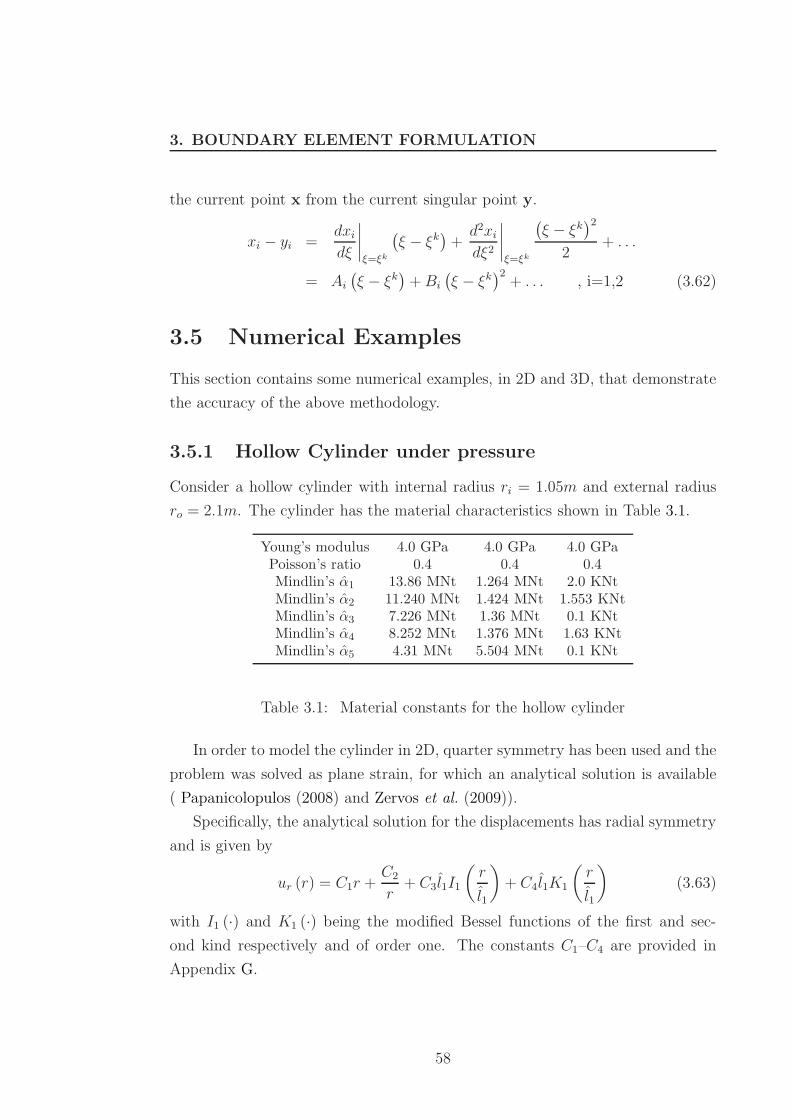
3.5.1 Hollow Cylinder under pressure . . . . . . . . . . . . . . . 56
3.5.2 Radial deformation of a Sphere . . . . . . . . . . . . . . . 58
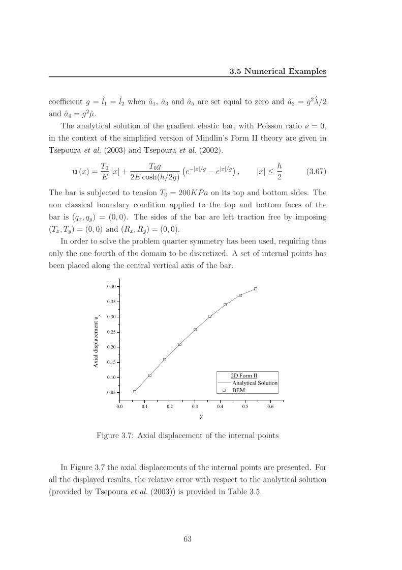
3.5.3 Tension of a bar . . . . . . . . . . . . . . . . . . . . . . . . 59
4 Fracture in Elasticity with Microstructure 63
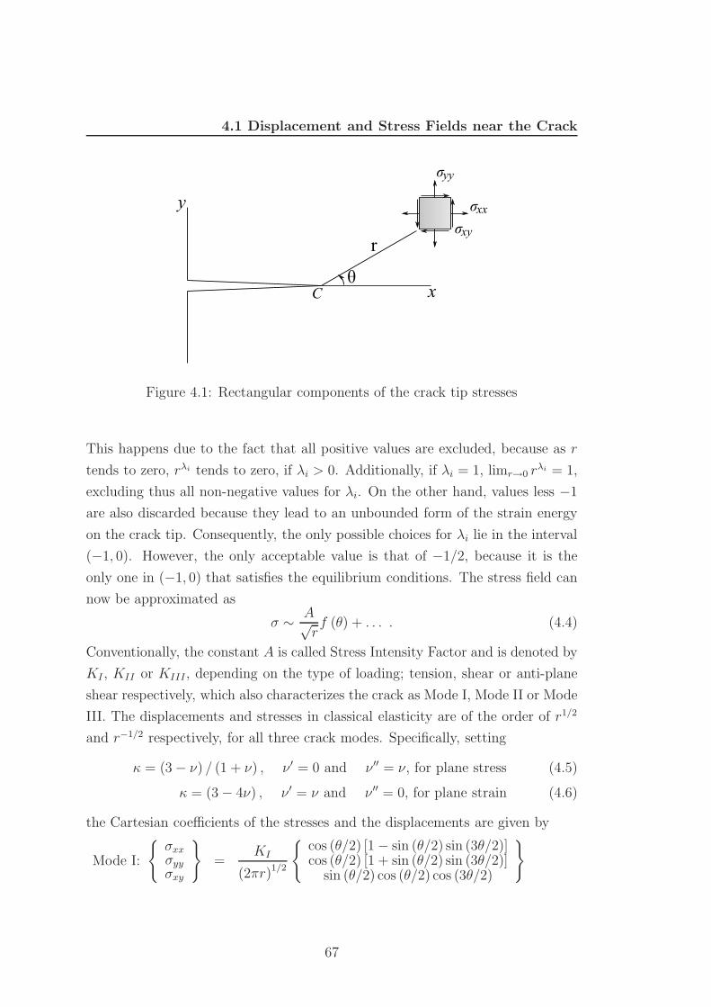
4.1 Displacement and Stress Fields near the Crack . . . . . . . . . . . 64
4.2 Crack Elements for Linear and Gradient Elastic Fracture . . . . . 67
4.2.1 Two dimensional crack element . . . . . . . . . . . . . . . 67
4.2.2 Integrations over a three noded quadratic line special element 71
4.2.2.1 Integrals involving the field R . . . . . . . . . . . 71
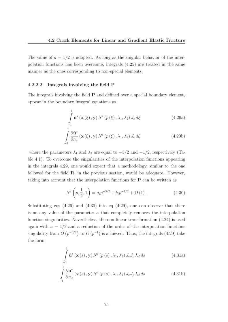
4.2.2.2 Integrals involving the field P . . . . . . . . . . . 73
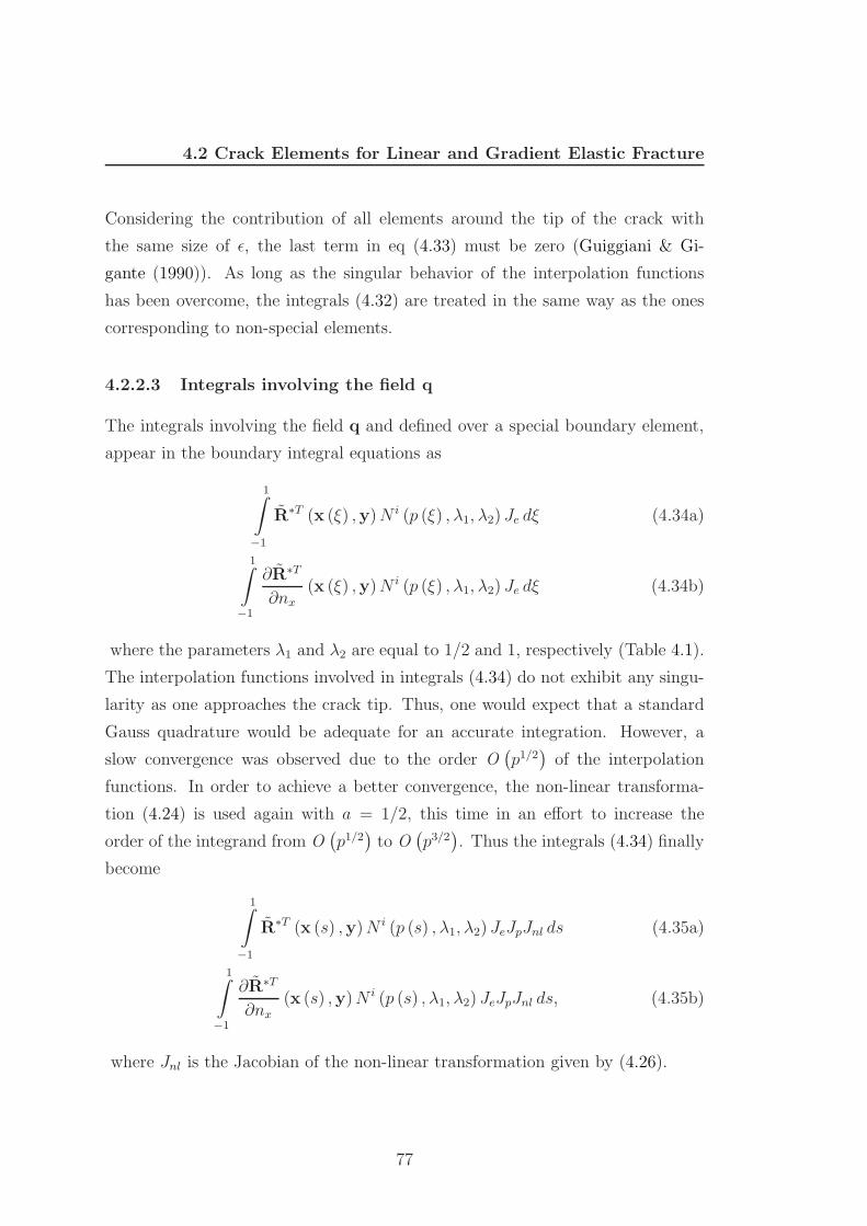
4.2.2.3 Integrals involving the field q . . . . . . . . . . . 75
4.2.3 Three dimensional crack element . . . . . . . . . . . . . . 75
4.2.4 Integrations over an eight-noded quadrilateral special element 78
4.2.4.1 Integrals involving the field R . . . . . . . . . . . 79
4.2.4.2 Integrals involving the field P . . . . . . . . . . . 80
4.2.4.3 Integrals involving the field q . . . . . . . . . . . 82
4.3 BEM Stress Intensity Factor Calculation . . . . . . . . . . . . . . 83
4.4 Numerical Examples . . . . . . . . . . . . . . . . . . . . . . . . . 84
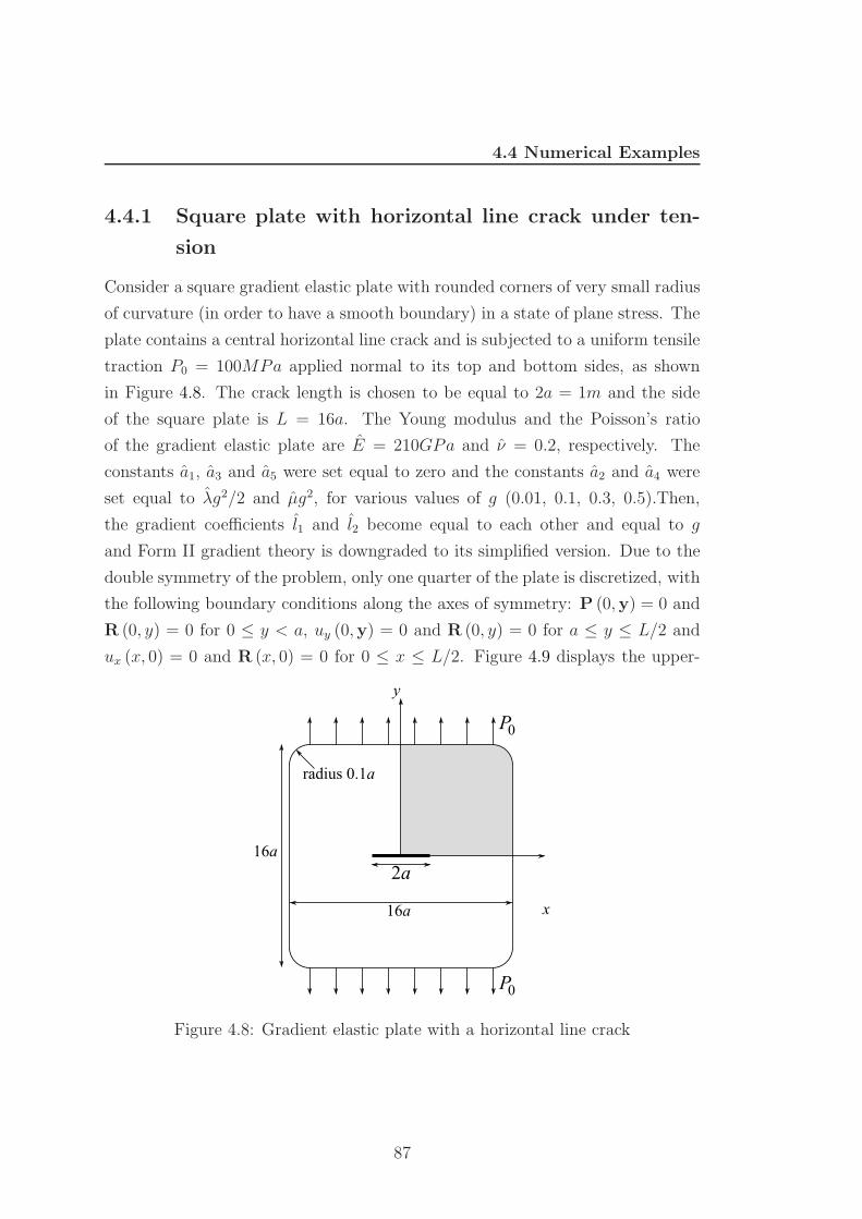
4.4.1 Square plate with horizontal line crack under tension . . . 85
4.4.2 Square plate with diagonal line crack under tension . . . . 90
4.4.3 Cube with central horizontal rectangular crack . . . . . . . 92
5 Conclusions and Future Work 97
A Form I, II & III Constants 101
A.1 Form I . . . . . . . . . . . . . . . . . . . . . . . . . . . . . . . . . 101
A.2 Form II . . . . . . . . . . . . . . . . . . . . . . . . . . . . . . . . 102
A.3 Form III . . . . . . . . . . . . . . . . . . . . . . . . . . . . . . . . 103
x
Page 13
CONTENTS
B Form II: Total Potential Energy Calculation 105
C Mindlin’s Form II: Kernels 107
D Boundary Elements 117
D.1 Surface Elements . . . . . . . . . . . . . . . . . . . . . . . . . . . 117
D.1.1 Eight Noded Quadratic Quadrilateral Element . . . . . . . 117
D.1.2 Six Noded Quadratic Triangular Element . . . . . . . . . . 120
D.2 Line Elements . . . . . . . . . . . . . . . . . . . . . . . . . . . . . 122
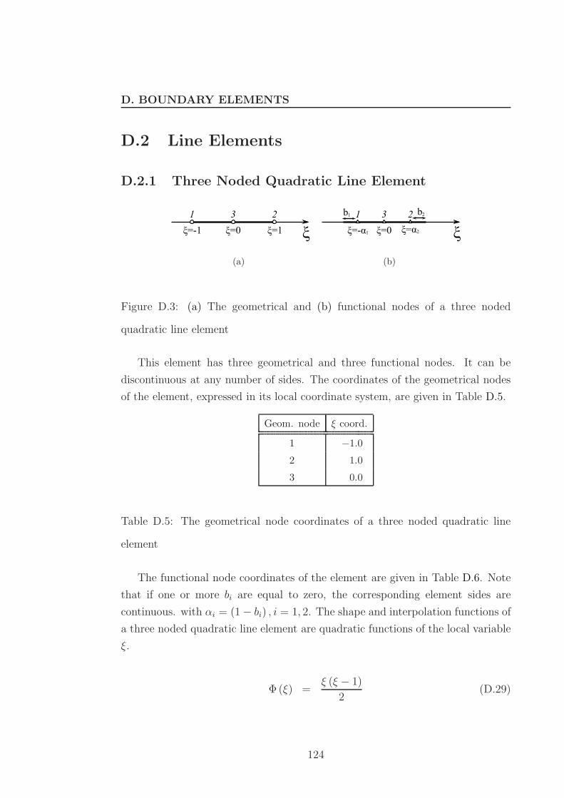
D.2.1 Three Noded Quadratic Line Element . . . . . . . . . . . . 122
E Diving elements into triangles 125
E.1 Quadrilateral Elements . . . . . . . . . . . . . . . . . . . . . . . . 125
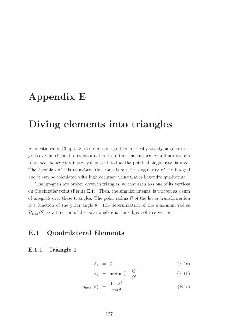
E.1.1 Triangle 1 . . . . . . . . . . . . . . . . . . . . . . . . . . . 125
E.1.2 Triangle 2 . . . . . . . . . . . . . . . . . . . . . . . . . . . 127
E.1.3 Triangle 3 . . . . . . . . . . . . . . . . . . . . . . . . . . . 127
E.1.4 Triangle 4 . . . . . . . . . . . . . . . . . . . . . . . . . . . 127
E.1.5 Triangle 5 . . . . . . . . . . . . . . . . . . . . . . . . . . . 128
E.1.6 Triangle 6 . . . . . . . . . . . . . . . . . . . . . . . . . . . 128
E.1.7 Triangle 7 . . . . . . . . . . . . . . . . . . . . . . . . . . . 128
E.1.8 Triangle 8 . . . . . . . . . . . . . . . . . . . . . . . . . . . 128
E.2 Triangular Elements . . . . . . . . . . . . . . . . . . . . . . . . . 129
E.2.1 Triangle 1 . . . . . . . . . . . . . . . . . . . . . . . . . . . 129
E.2.2 Triangle 2 . . . . . . . . . . . . . . . . . . . . . . . . . . . 130
E.2.3 Triangle 3 . . . . . . . . . . . . . . . . . . . . . . . . . . . 130
E.2.4 Triangle 4 . . . . . . . . . . . . . . . . . . . . . . . . . . . 131
E.2.5 Triangle 5 . . . . . . . . . . . . . . . . . . . . . . . . . . . 131
E.2.6 Triangle 6 . . . . . . . . . . . . . . . . . . . . . . . . . . . 132
F Taylor expansion of the position vector 133
G Hollow Cylinder Under Pressure: Analytical solution constants135
H Eight Noded Special Element: Interpolation Functions 137
References 153
xi
Page 15
List of Figures
2.1 The one dimensional continuum . . . . . . . . . . . . . . . . . . . 11
2.2 1D continuum with quadratically varying displacements and smaller
element size . . . . . . . . . . . . . . . . . . . . . . . . . . . . . . 12
2.3 Kinematic parameters of Mindlin’s theory of elasticity with mi-
crostructure . . . . . . . . . . . . . . . . . . . . . . . . . . . . . . 15
2.4 Typical components of the double stress tensor and gradient micro-
deformation . . . . . . . . . . . . . . . . . . . . . . . . . . . . . . 16
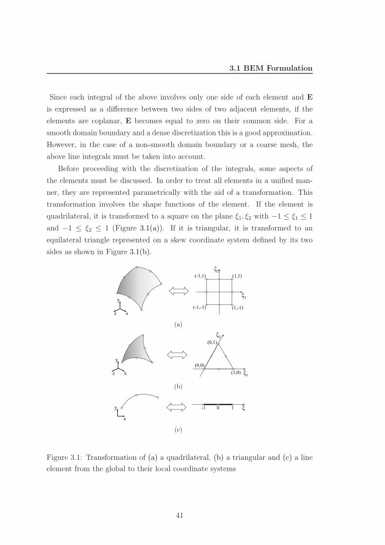
3.1 Transformation of elements from the global to their local coordi-
nate system . . . . . . . . . . . . . . . . . . . . . . . . . . . . . . 39
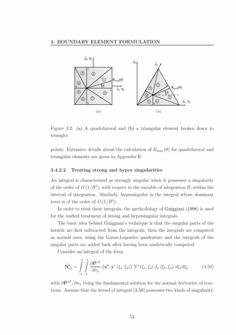
3.2 Elements broken down to triangles . . . . . . . . . . . . . . . . . 52
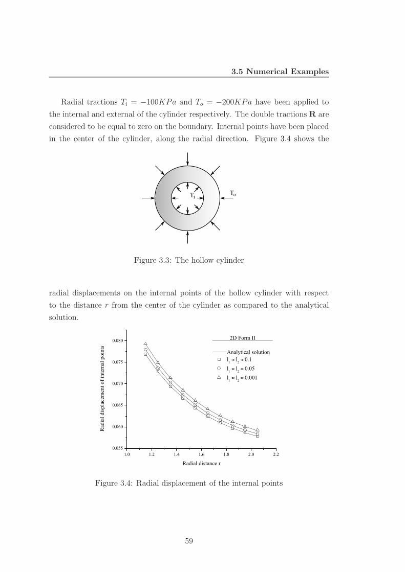
3.3 The hollow cylinder . . . . . . . . . . . . . . . . . . . . . . . . . . 57
3.4 Radial displacement of the internal points . . . . . . . . . . . . . 57
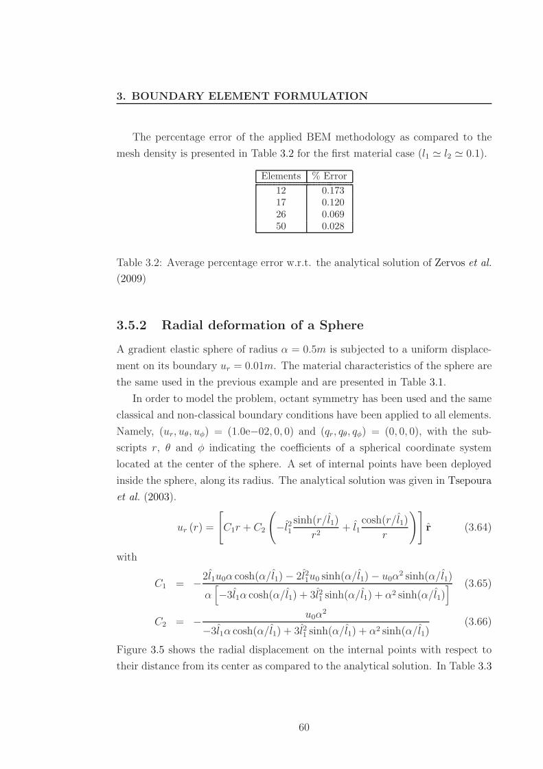
3.5 Radial displacement of the internal points . . . . . . . . . . . . . 59
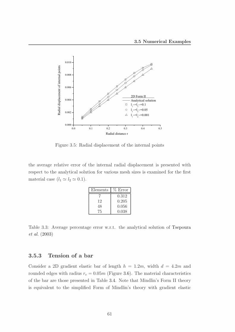
3.6 The gradient elastic bar . . . . . . . . . . . . . . . . . . . . . . . 60
3.7 Axial displacement of the internal points . . . . . . . . . . . . . . 61
4.1 Rectangular components of the crack tip stresses . . . . . . . . . . 64
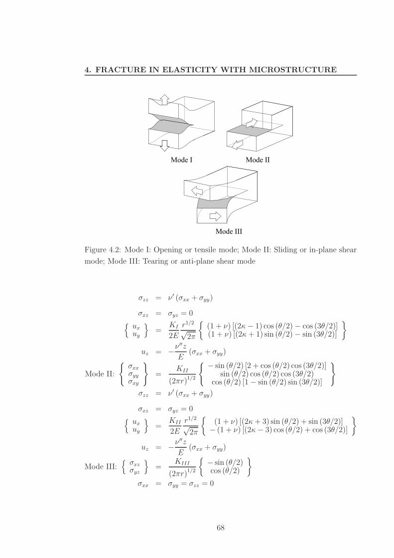
4.2 Mode I: Opening or tensile mode; Mode II: Sliding or in-plane
shear mode; Mode III: Tearing or anti-plane shear mode . . . . . 66
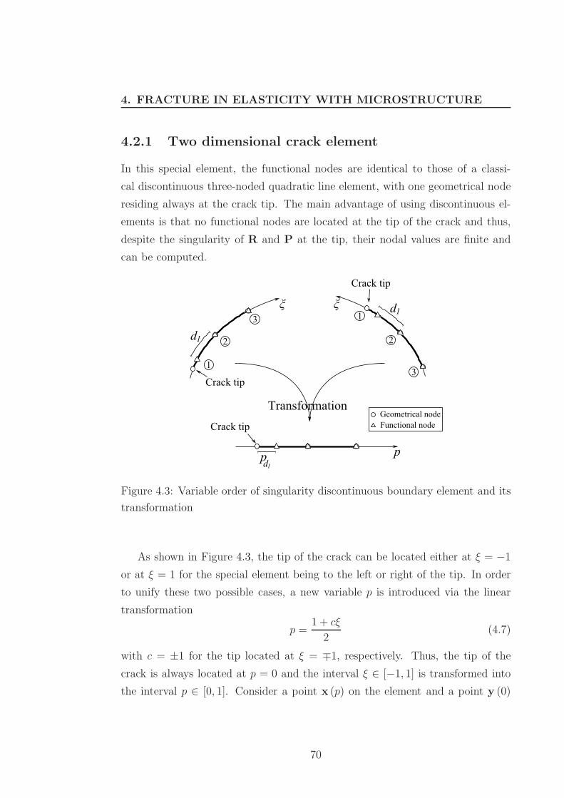
4.3 Variable order of singularity discontinuous boundary element and
its transformation . . . . . . . . . . . . . . . . . . . . . . . . . . . 68
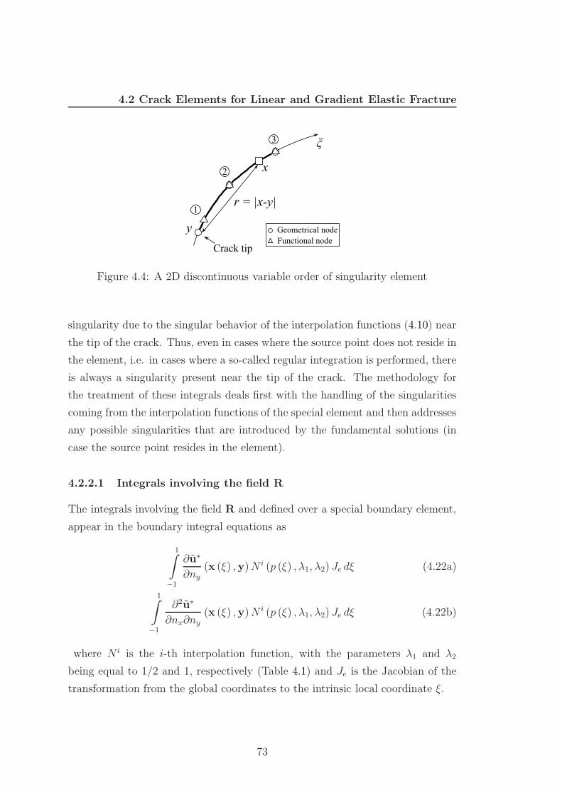
4.4 A 2D discontinuous variable order of singularity element . . . . . 70
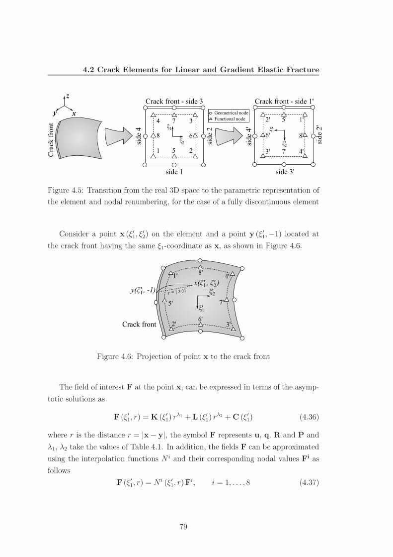
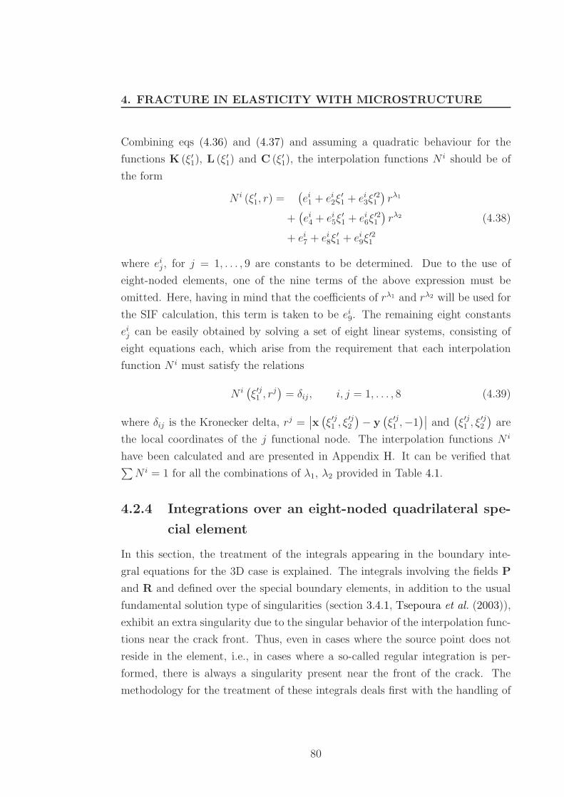
4.5 Transition from the real 3D space to the parametric representa-
tion of the element and nodal renumbering, for the case of a fully
discontinuous element . . . . . . . . . . . . . . . . . . . . . . . . . 77
xiii
Page 16
LIST OF FIGURES
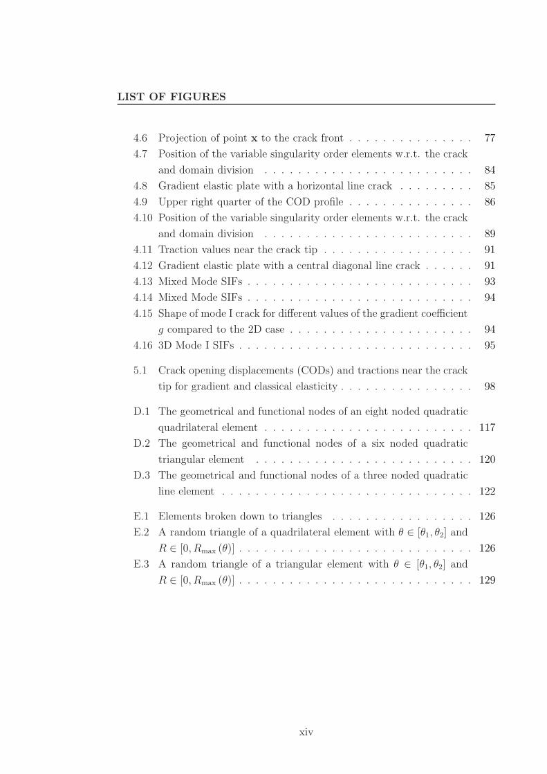
4.6 Projection of point x to the crack front . . . . . . . . . . . . . . . 77
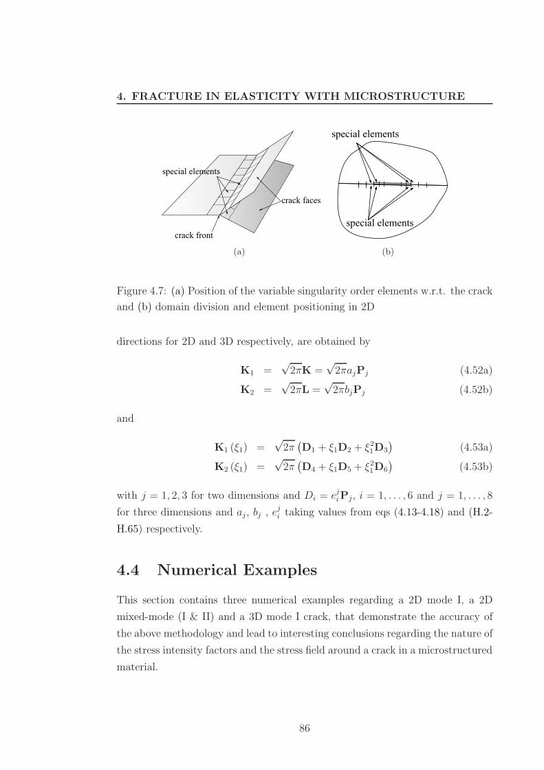
4.7 Position of the variable singularity order elements w.r.t. the crack
and domain division . . . . . . . . . . . . . . . . . . . . . . . . . 84
4.8 Gradient elastic plate with a horizontal line crack . . . . . . . . . 85
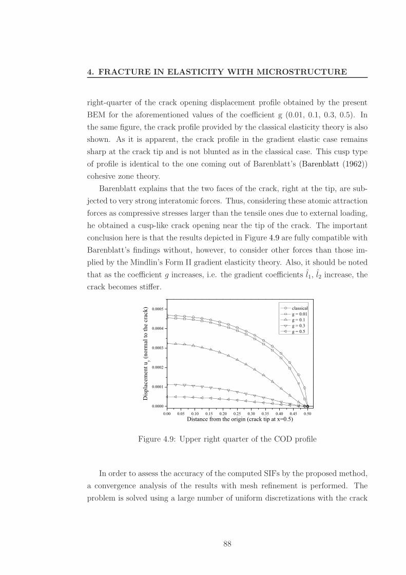
4.9 Upper right quarter of the COD profile . . . . . . . . . . . . . . . 86
4.10 Position of the variable singularity order elements w.r.t. the crack
and domain division . . . . . . . . . . . . . . . . . . . . . . . . . 89
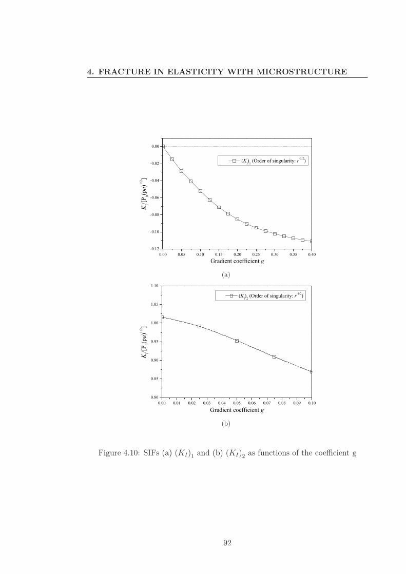
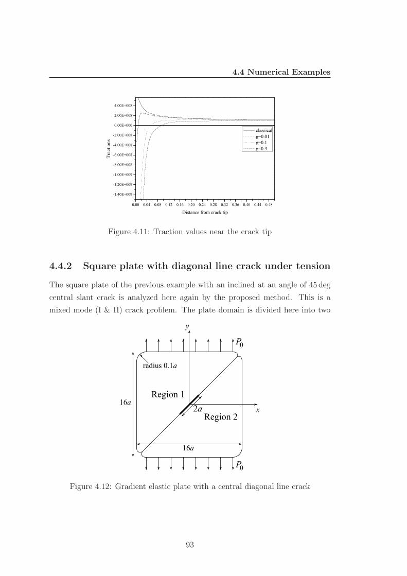
4.11 Traction values near the crack tip . . . . . . . . . . . . . . . . . . 91
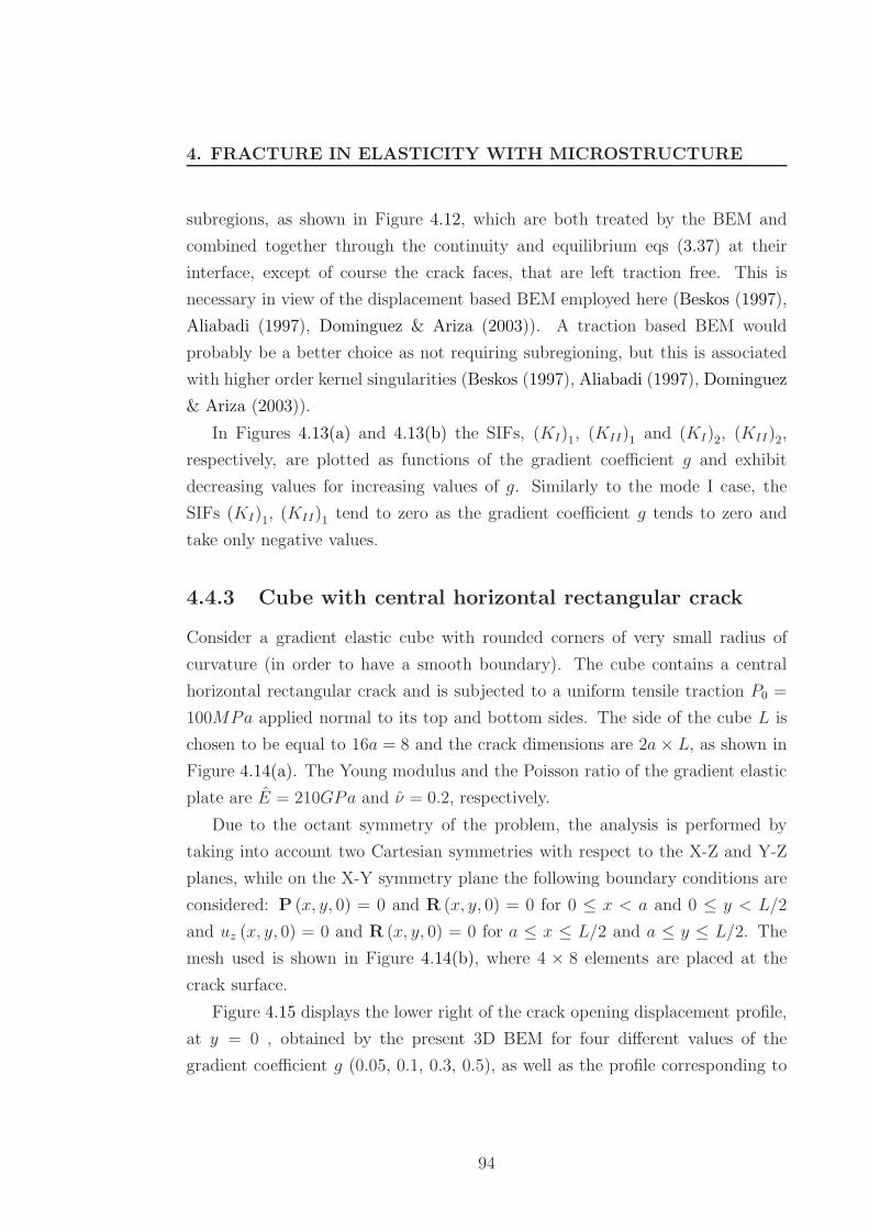
4.12 Gradient elastic plate with a central diagonal line crack . . . . . . 91
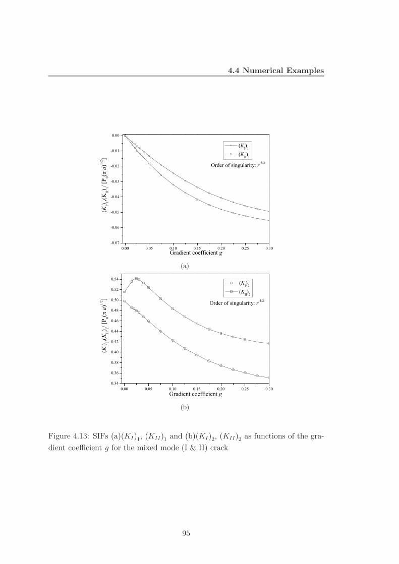
4.13 Mixed Mode SIFs . . . . . . . . . . . . . . . . . . . . . . . . . . . 93
4.14 Mixed Mode SIFs . . . . . . . . . . . . . . . . . . . . . . . . . . . 94
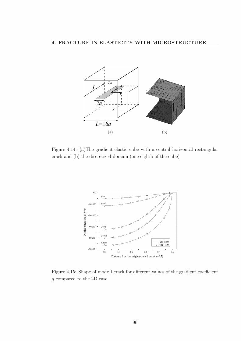
4.15 Shape of mode I crack for different values of the gradient coefficient
g compared to the 2D case . . . . . . . . . . . . . . . . . . . . . . 94
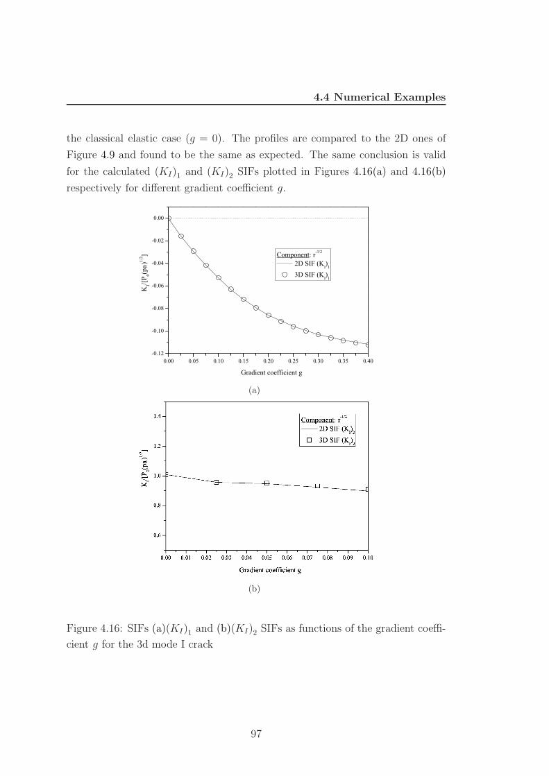
4.16 3D Mode I SIFs . . . . . . . . . . . . . . . . . . . . . . . . . . . . 95
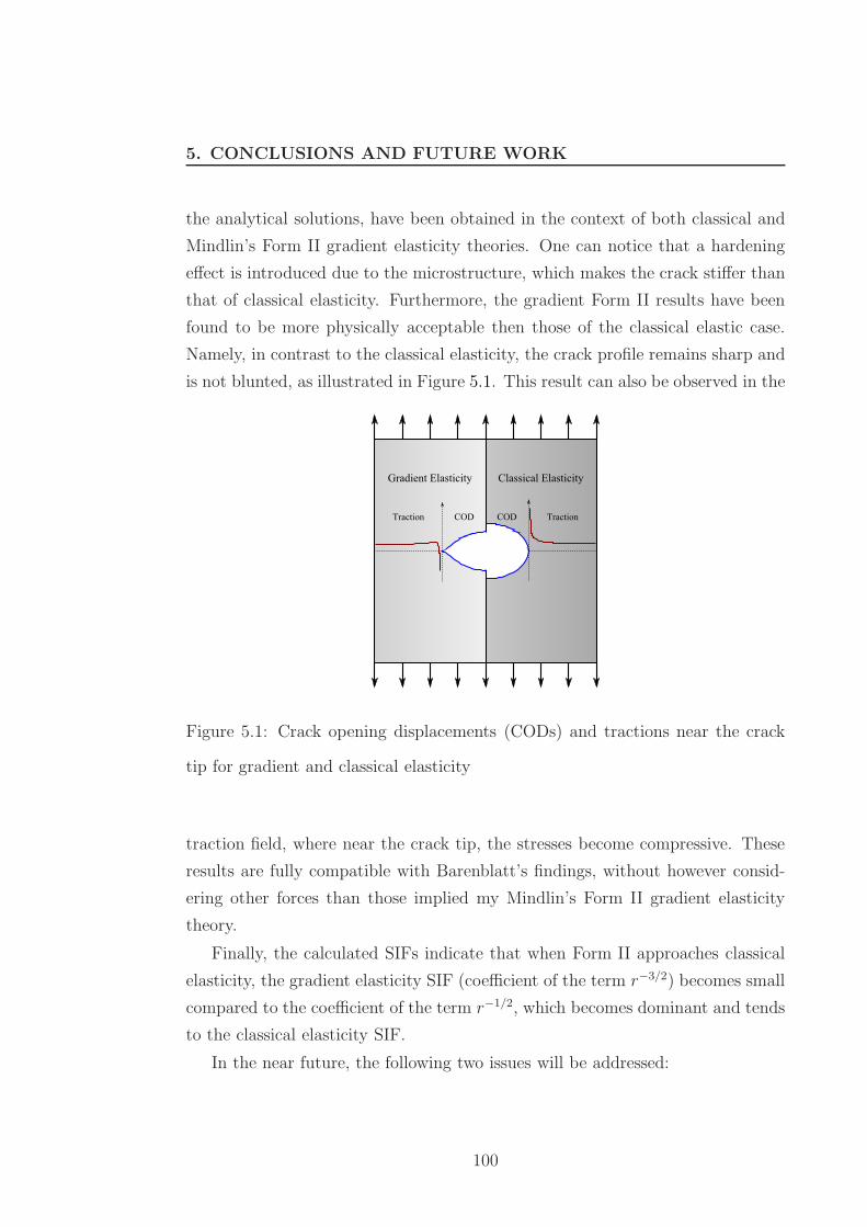
5.1 Crack opening displacements (CODs) and tractions near the crack
tip for gradient and classical elasticity . . . . . . . . . . . . . . . . 98
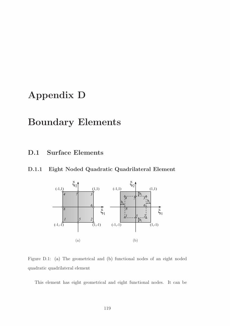
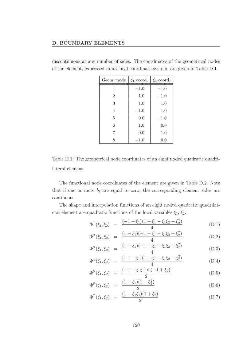
D.1 The geometrical and functional nodes of an eight noded quadratic
quadrilateral element . . . . . . . . . . . . . . . . . . . . . . . . . 117
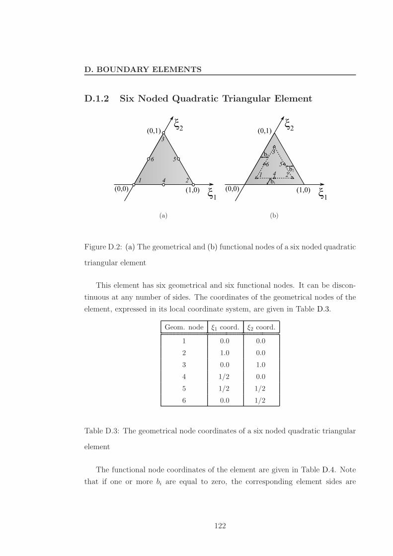
D.2 The geometrical and functional nodes of a six noded quadratic
triangular element . . . . . . . . . . . . . . . . . . . . . . . . . . 120
D.3 The geometrical and functional nodes of a three noded quadratic
line element . . . . . . . . . . . . . . . . . . . . . . . . . . . . . . 122
E.1 Elements broken down to triangles . . . . . . . . . . . . . . . . . 126
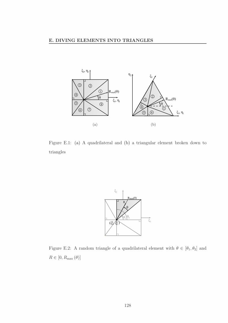
E.2 A random triangle of a quadrilateral element with θ ∈ [θ1, θ2] and
R ∈ [0, Rmax (θ)] . . . . . . . . . . . . . . . . . . . . . . . . . . . . 126
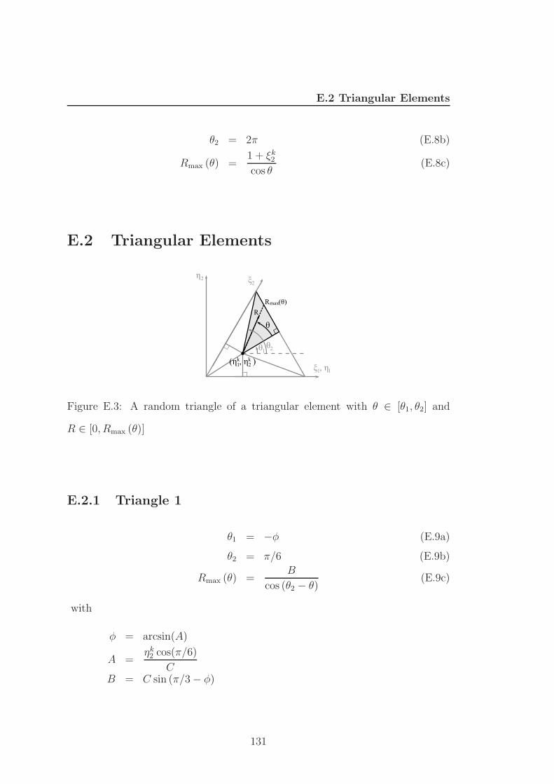
E.3 A random triangle of a triangular element with θ ∈ [θ1, θ2] and
R ∈ [0, Rmax (θ)] . . . . . . . . . . . . . . . . . . . . . . . . . . . . 129
xiv
Page 17
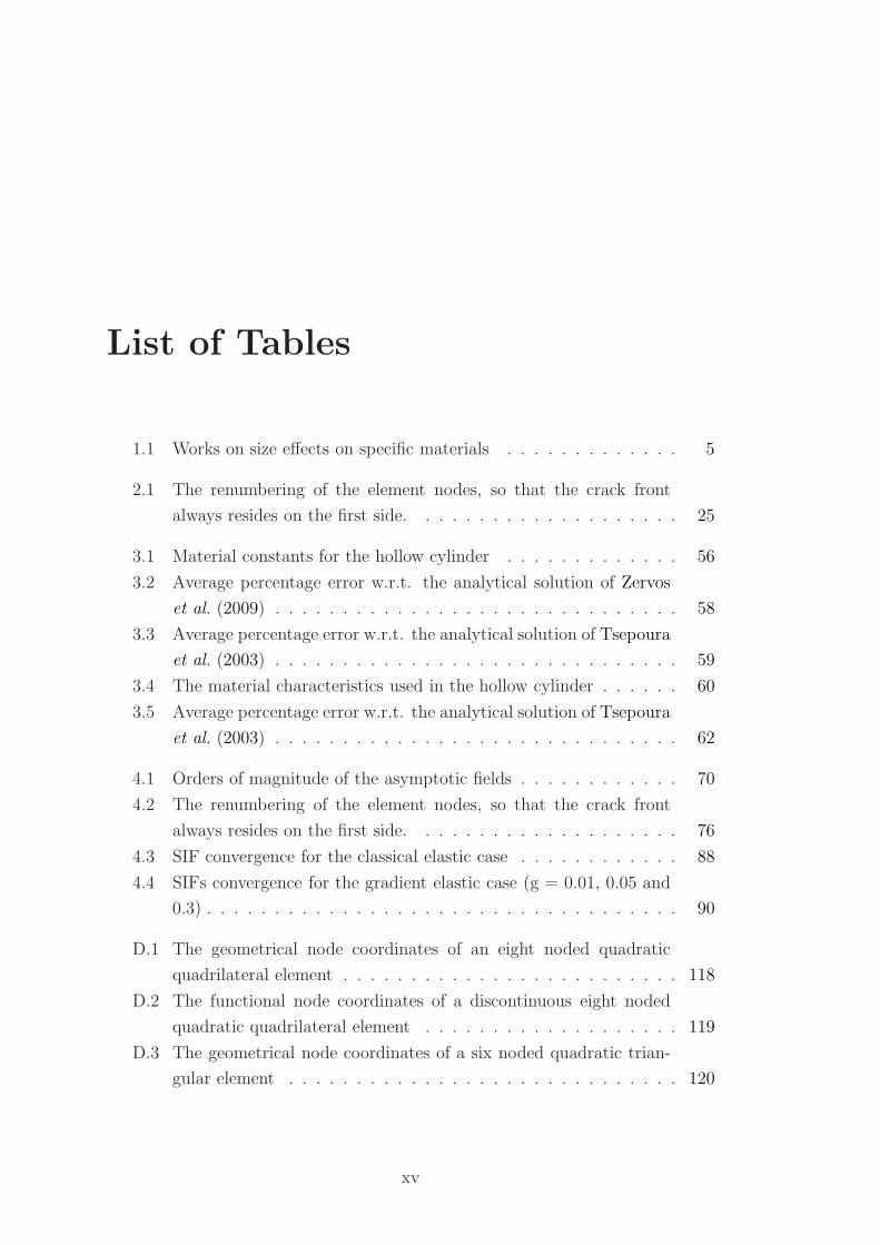
List of Tables
1.1 Works on size effects on specific materials . . . . . . . . . . . . . 5
2.1 The renumbering of the element nodes, so that the crack front
always resides on the first side. . . . . . . . . . . . . . . . . . . . 25
3.1 Material constants for the hollow cylinder . . . . . . . . . . . . . 56
3.2 Average percentage error w.r.t. the analytical solution of Zervos
et al. (2009) . . . . . . . . . . . . . . . . . . . . . . . . . . . . . . 58
3.3 Average percentage error w.r.t. the analytical solution of Tsepoura
et al. (2003) . . . . . . . . . . . . . . . . . . . . . . . . . . . . . . 59
3.4 The material characteristics used in the hollow cylinder . . . . . . 60
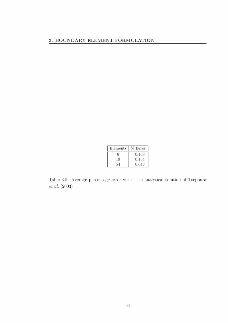
3.5 Average percentage error w.r.t. the analytical solution of Tsepoura
et al. (2003) . . . . . . . . . . . . . . . . . . . . . . . . . . . . . . 62
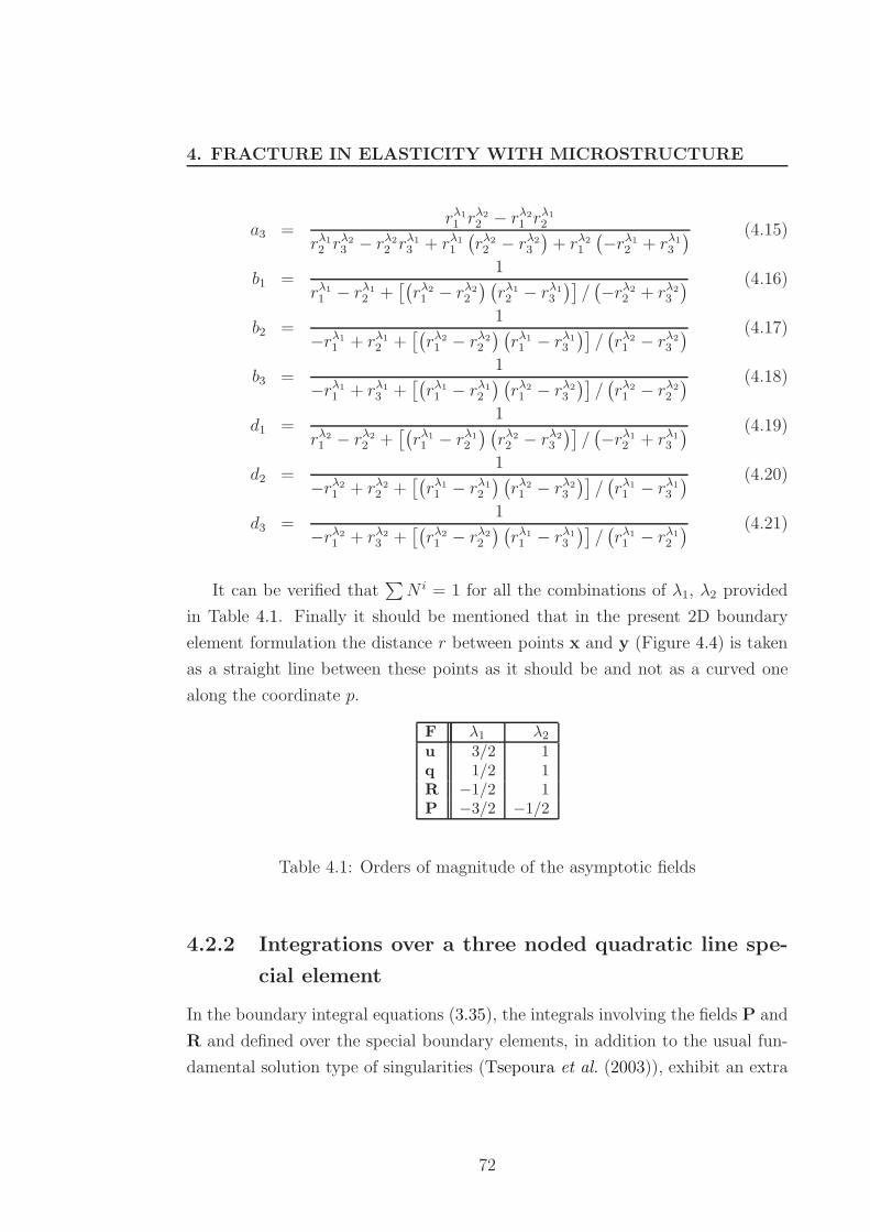
4.1 Orders of magnitude of the asymptotic fields . . . . . . . . . . . . 70
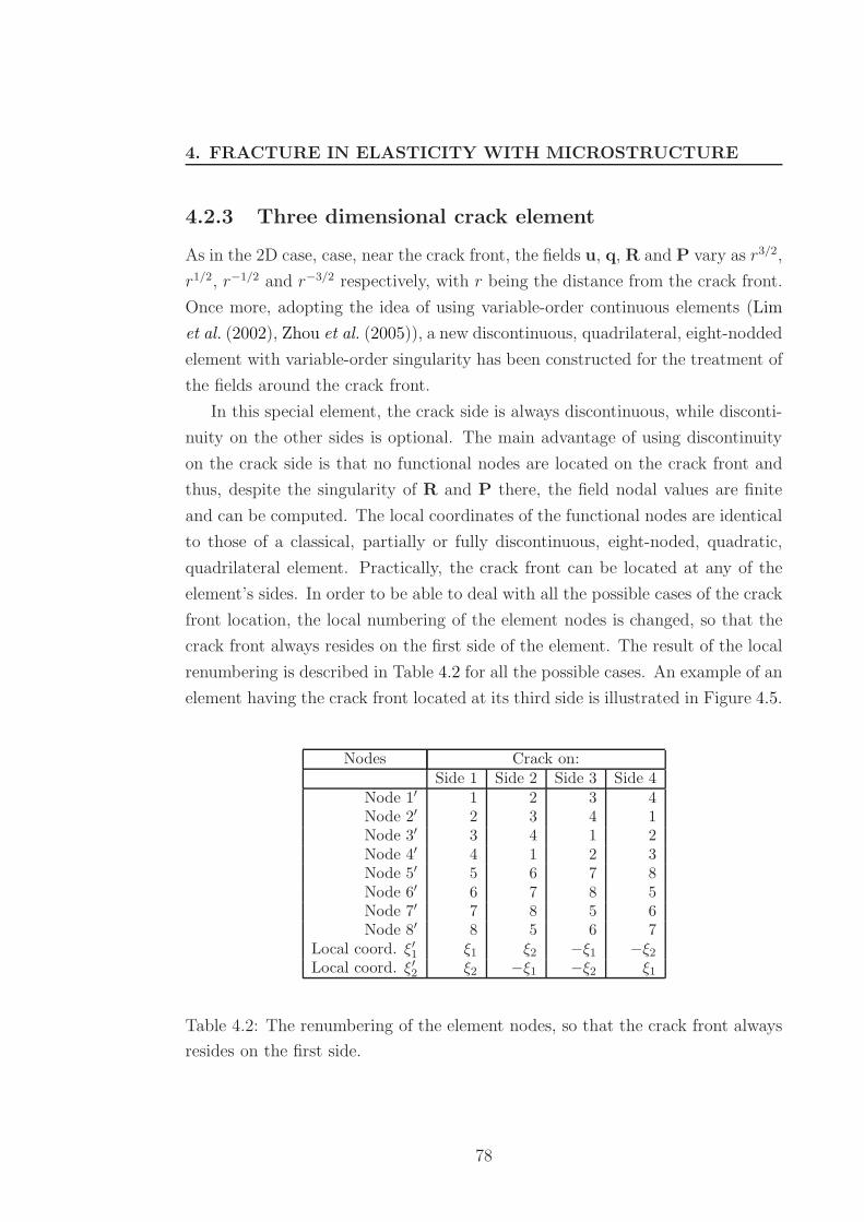
4.2 The renumbering of the element nodes, so that the crack front
always resides on the first side. . . . . . . . . . . . . . . . . . . . 76
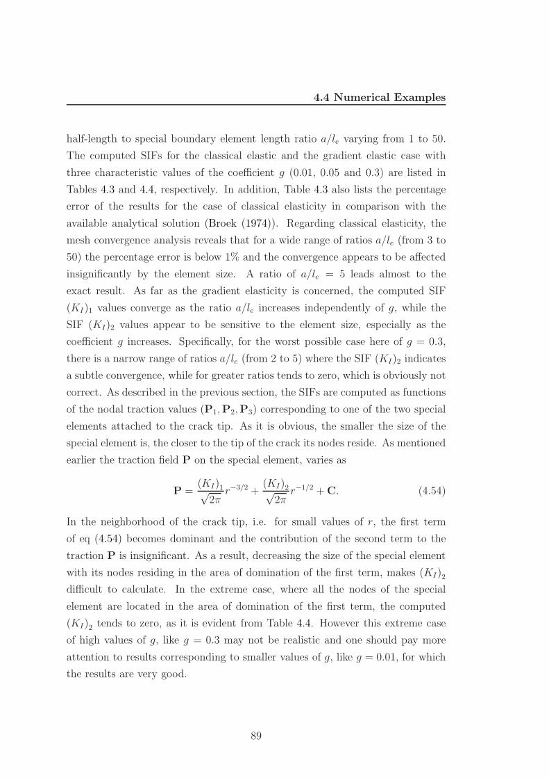
4.3 SIF convergence for the classical elastic case . . . . . . . . . . . . 88
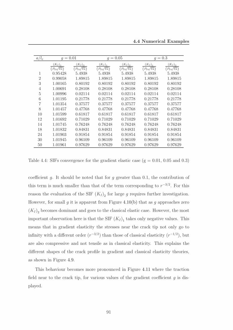
4.4 SIFs convergence for the gradient elastic case (g = 0.01, 0.05 and
0.3) . . . . . . . . . . . . . . . . . . . . . . . . . . . . . . . . . . . 90
D.1 The geometrical node coordinates of an eight noded quadratic
quadrilateral element . . . . . . . . . . . . . . . . . . . . . . . . . 118
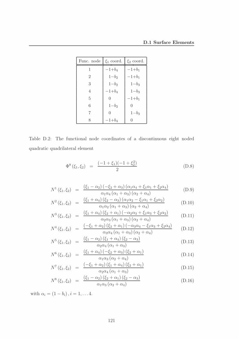
D.2 The functional node coordinates of a discontinuous eight noded
quadratic quadrilateral element . . . . . . . . . . . . . . . . . . . 119
D.3 The geometrical node coordinates of a six noded quadratic trian-
gular element . . . . . . . . . . . . . . . . . . . . . . . . . . . . . 120
xv
Page 18
LIST OF TABLES
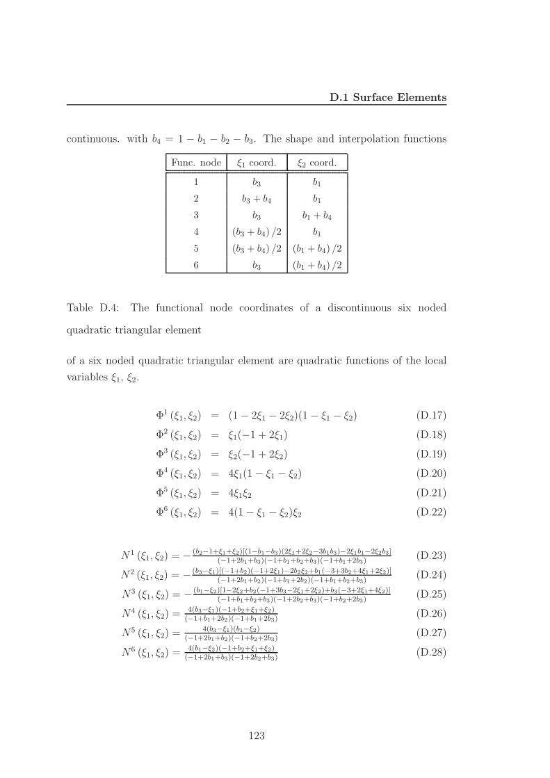
D.4 The functional node coordinates of a discontinuous six noded quadratic
triangular element . . . . . . . . . . . . . . . . . . . . . . . . . . 121
D.5 The geometrical node coordinates of a three noded quadratic line
element . . . . . . . . . . . . . . . . . . . . . . . . . . . . . . . . 122
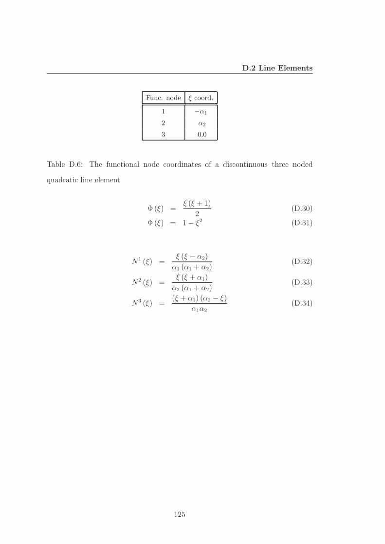
D.6 The functional node coordinates of a discontinuous three noded
quadratic line element . . . . . . . . . . . . . . . . . . . . . . . . 123
xvi
Page 19
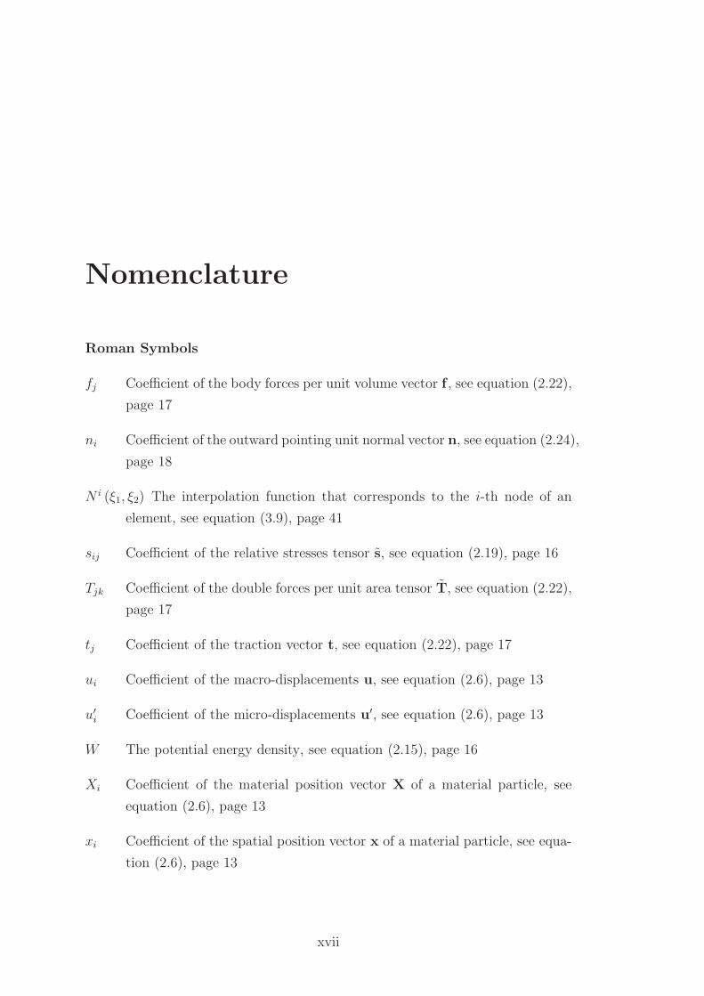
Nomenclature
Roman Symbols
fj Coefficient of the body forces per unit volume vector f , see equation (2.22),
page 17
ni Coefficient of the outward pointing unit normal vector n, see equation (2.24),
page 18
N i (ξ1, ξ2) The interpolation function that corresponds to the i-th node of an
element, see equation (3.9), page 41
sij Coefficient of the relative stresses tensor s, see equation (2.19), page 16
Tjk Coefficient of the double forces per unit area tensor T, see equation (2.22),
page 17
tj Coefficient of the traction vector t, see equation (2.22), page 17
ui Coefficient of the macro-displacements u, see equation (2.6), page 13
u′i Coefficient of the micro-displacements u′, see equation (2.6), page 13
W The potential energy density, see equation (2.15), page 16
Xi Coefficient of the material position vector X of a material particle, see
equation (2.6), page 13
xi Coefficient of the spatial position vector x of a material particle, see equa-
tion (2.6), page 13
xvii
Page 20
NOMENCLATURE
X ′i Coefficient of the material position vector X′ of a material particle with
respect to a rectangular coordinate system that has its origin fixed in the
particle, see equation (2.6), page 13
x′i Coefficient of the spatial position vector x′ of a material particle with
respect to a rectangular coordinate system that has its origin fixed in the
particle, see equation (2.6), page 13
Greek Symbols
ǫij Coefficient of the macro-strain tensor ǫ, see equation (2.12), page 14
γij Coefficient of the relative deformation tensor γ, see equation (2.13), page 15
κijk Coefficient of the micro-deformation gradient ˜κ, see equation (2.14), page 15
λ, µ Lame constants
µijk Coefficient of the double stresses tensor ˜µ, see equation (2.19), page 16
ωij Coefficient of the macro-rotation tensor ω, see equation (2.12), page 14
Φjk Coefficient of the double forces per unit volume tensor Φ, see equation (2.22),
page 17
Φi (ξ1, ξ2) The shape function that corresponds to the i-th node of an element,
see equation (3.4), page 40
ψjk Coefficient of the micro-deformation ψ, see equation (2.9), page 14
σij Coefficient of the total stresses tensor σ, see equation (2.19), page 16
τij Coefficient of the Cauchy stresses tensor τ , see equation (2.19), page 16
Subscripts
L[i,j] The anti-symmetric part of second order tensor L
L(i,j) The symmetric part of second order tensor L
xviii
Page 21
Chapter 1
Introduction
1.1 Linear elastic theories with microstructural
effects
Experimental observations have shown that macroscopically many materials are
significantly affected by their microstructure and exhibit a mechanical behavior
which is different than that expected classically. Polycrystals, polymers, metal-
lic and polymeric foams, granular materials, graphite, concrete, asphalt, porous
media, cellular materials, bones and particle or fiber reinforced composites are
some examples of such materials. These microstructural effects become more
pronounced especially when the size or a dimension of the considered structure
becomes small and comparable to the microstructure of the constituent materials.
Representative examples are those of membranes, very thin plates and shells, mi-
croelectronic devices, micromechanical systems, layered plates, bones and smart
structures. However, even in large structures there are mechanical responses lo-
calized to small areas of the structural material (cracks, shear bands, dislocations)
the size of which is comparable to the dimensions of the microstructure. Some
representative works dealing with size effects in the aforementioned materials are
provided in Table 1.1.
Due to the lack of internal parameters, which would correlate the microstruc-
ture with the macrostructure, classical theory of linear elasticity fails to describe
such behavior. Thus, resort should be made to other enhanced elastic theories
1
Page 22
1. INTRODUCTION
where internal length scale constants correlating the microscopic representative
volume elements with the macrostructure are involved in the constitutive equa-
tions of the considered elastic continuum. Such theories and the most general are
the Cosserat elasticity theory (Cosserat & Cosserat (1909)), the Cosserat the-
ory with constrained rotations or couple stresses theory (Grioli (1960), Toupin
(1962), Mindlin & Tiersten (1962), Koiter (1964)), the strain gradient theory
(Toupin (1964)), the multipolar theory of continuum mechanics (Green & Rivlin
(1964)), the elastic theory with microstructure (Mindlin (1964), Mindlin (1965)),
the micromorphic, microstretch and micropolar elastic theories (Eringen (1999))
and the non-local elasticity (Eringen (1992)). Most of the aforementioned the-
ories have been developed in the decade of 60’s and excellent historical reviews
and comments on the subject can be found in the review articles of Mindlin
& Tiersten (1962) and Tiersten & Bleustein (1974), in the paper of Exadakty-
los & Vardoulakis (2001), in the thesis of Tekoglou (2007) and in the books of
Vardoulakis & Sulem (1995) and Eringen (1999).
Cosserat brothers were the first to develop a general mechanics framework of
continuous media where each point possesses six degrees of freedom like a rigid
body and not three (position of a point in Euclidean space) as the classical elas-
ticity does. These three extra degrees of freedom correspond to three directors,
which represent rotations created by the so called “couple stresses”. As mentioned
by Toupin (1964), the most novel feature of Cosserat theory is the appearance
of couple stresses in the equilibrium equations and equations of motion. How-
ever, although this theory is a landmark in the development of enhanced elastic
theories, it did not receive much attention due to the lack of specific constitutive
relations and the non-symmetry of the considered stresses. By the end of the 50’s
and during the beginning of 60’s the subject of the theory of elasticity with couple
stresses reopened and a plethora of new couple stresses elastic theories were pro-
posed in the literature (Grioli (1960), Toupin (1964), Mindlin & Tiersten (1962),
Koiter (1964)). Most of them explored the special case where the three rotations
coincide with the local rotations of classical elasticity leading thus to a couple
stresses theory with three independent variables, i.e. the three components of dis-
placement vector. Using this consideration, beyond the six components of strains,
other eight of the eighteen components of the first gradient of strain were inserted
2
Page 23
1.1 Linear elastic theories with microstructural effects
in the expression of the strain energy density function. All the components of the
first gradient of the strain were introduced into the strain energy density function,
in a non-linear fashion, by Toupin (1964) proposing the strain gradient theory.
Considering higher order gradients of strains, Green & Rivlin (1964) developed a
very complicated, but the most general enhanced theory of elasticity called mul-
tipolar theory of continuum mechanics. In 1964 and 1965 Mindlin developed a
general and comprehensive elastic theory with microstructure which is actually
the linear version of Toupin’s strain gradient theory and equivalent to the dipolar
gradient theory of Green and Rivlin. In order to balance the dimensions of strains
and higher order gradients of strains as well as to correlate the micro-strains with
macro-strains, Mindlin (1964) utilized eighteen new constants rendering thus his
general theory very complicated from physical and mathematical point of view.
In the sequel, considering long wave-lengths and the same deformation for macro
and micro structure Mindlin proposed three new simplified versions of his theory,
known as Form I, II and III, utilizing in the constitutive equations seven material
and internal length scale parameters instead of eighteen employed in his initial
model. In Form-I, the strain energy density function is assumed to be a quadratic
form of the classical strains and the second gradient of displacement; in Form II
the second displacement gradient is replaced by the gradient of strains and in
Form III the strain energy function is written in terms of the strain, the gradient
of rotation, and the fully symmetric part of the gradient of strain. Although the
three forms are equivalent to each other and conclude to the same equation of
motion, the Form-II leads to a symmetric total stress tensor, as in the case of clas-
sical elasticity, avoiding thus the problems associated with non-symmetric stress
tensors introduced by Cosserat and couple stress theories. Almost simultane-
ously with Mindlin, Eringen (see Eringen (1999)) proposed three general elastic
theories with microstructural considerations called micromorphic, microstretch
and micropolar theories. The micromorphic continuum is none other than the
classical continuum endowed with extra degrees of freedom represented by three
deformable directors, which represent the degrees of freedom arising from mi-
crodeformations of the physical particle. The linear form of the micromorphic
theory (see Eringen (1999)) coincides with the micro-structure theory of Mindlin
3
Page 24
1. INTRODUCTION
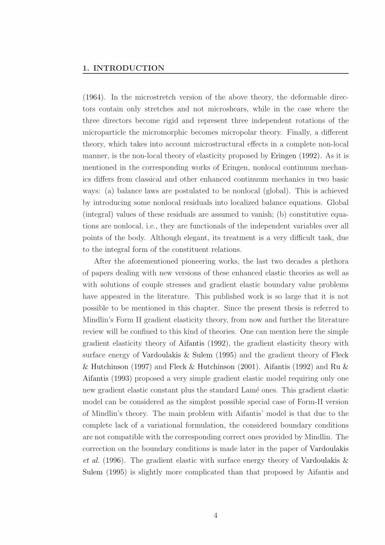
(1964). In the microstretch version of the above theory, the deformable direc-
tors contain only stretches and not microshears, while in the case where the
three directors become rigid and represent three independent rotations of the
microparticle the micromorphic becomes micropolar theory. Finally, a different
theory, which takes into account microstructural effects in a complete non-local
manner, is the non-local theory of elasticity proposed by Eringen (1992). As it is
mentioned in the corresponding works of Eringen, nonlocal continuum mechan-
ics differs from classical and other enhanced continuum mechanics in two basic
ways: (a) balance laws are postulated to be nonlocal (global). This is achieved
by introducing some nonlocal residuals into localized balance equations. Global
(integral) values of these residuals are assumed to vanish; (b) constitutive equa-
tions are nonlocal, i.e., they are functionals of the independent variables over all
points of the body. Although elegant, its treatment is a very difficult task, due
to the integral form of the constituent relations.
After the aforementioned pioneering works, the last two decades a plethora
of papers dealing with new versions of these enhanced elastic theories as well as
with solutions of couple stresses and gradient elastic boundary value problems
have appeared in the literature. This published work is so large that it is not
possible to be mentioned in this chapter. Since the present thesis is referred to
Mindlin’s Form II gradient elasticity theory, from now and further the literature
review will be confined to this kind of theories. One can mention here the simple
gradient elasticity theory of Aifantis (1992), the gradient elasticity theory with
surface energy of Vardoulakis & Sulem (1995) and the gradient theory of Fleck
& Hutchinson (1997) and Fleck & Hutchinson (2001). Aifantis (1992) and Ru &
Aifantis (1993) proposed a very simple gradient elastic model requiring only one
new gradient elastic constant plus the standard Lame ones. This gradient elastic
model can be considered as the simplest possible special case of Form-II version
of Mindlin’s theory. The main problem with Aifantis’ model is that due to the
complete lack of a variational formulation, the considered boundary conditions
are not compatible with the corresponding correct ones provided by Mindlin. The
correction on the boundary conditions is made later in the paper of Vardoulakis
et al. (1996). The gradient elastic with surface energy theory of Vardoulakis &
Sulem (1995) is slightly more complicated than that proposed by Aifantis and
4
Page 25
1.2 Numerical solutions in gradient elastic theories
co-workers but it is a direct consequence of the continuum model proposed by
Casal (1972) and not a special case of Mindlin’s general theory. Finally, Fleck
& Hutchinson (1997) and Fleck & Hutchinson (2001) decomposed the second
gradient of displacement into the stretch gradient and the rotation gradient ten-
sors proposing thus an alternative version of Mindlin’s Form I gradient elasticity
theory.
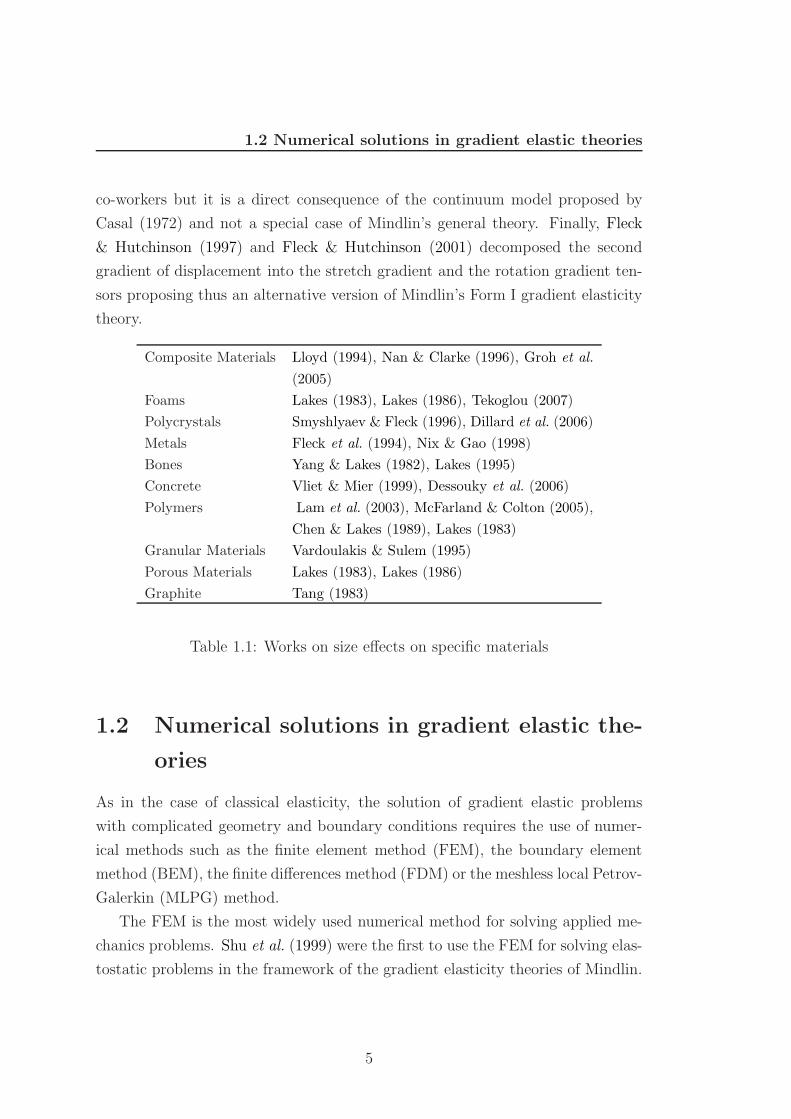
Composite Materials Lloyd (1994), Nan & Clarke (1996), Groh et al.
(2005)
Foams Lakes (1983), Lakes (1986), Tekoglou (2007)
Polycrystals Smyshlyaev & Fleck (1996), Dillard et al. (2006)
Metals Fleck et al. (1994), Nix & Gao (1998)
Bones Yang & Lakes (1982), Lakes (1995)
Concrete Vliet & Mier (1999), Dessouky et al. (2006)
Polymers Lam et al. (2003), McFarland & Colton (2005),
Chen & Lakes (1989), Lakes (1983)
Granular Materials Vardoulakis & Sulem (1995)
Porous Materials Lakes (1983), Lakes (1986)
Graphite Tang (1983)
Table 1.1: Works on size effects on specific materials
1.2 Numerical solutions in gradient elastic the-
ories
As in the case of classical elasticity, the solution of gradient elastic problems
with complicated geometry and boundary conditions requires the use of numer-
ical methods such as the finite element method (FEM), the boundary element
method (BEM), the finite differences method (FDM) or the meshless local Petrov-
Galerkin (MLPG) method.
The FEM is the most widely used numerical method for solving applied me-
chanics problems. Shu et al. (1999) were the first to use the FEM for solving elas-
tostatic problems in the framework of the gradient elasticity theories of Mindlin.
5
Page 26
1. INTRODUCTION
Since then, many papers dealing with FEM solutions of gradient elastic problems
have appeared in the literature. Here one can mention the FEM formulations
of Amanatidou & Aravas (2002), Engel et al. (2002), Tenek & Aifantis (2002),
Matsushima et al. (2002), Peerlings & Fleck (2004), Soh & Wanji (2004), Imatani
et al. (2005), Askes & Gutierrez (2006), Dessouky et al. (2003), Dessouky et al.
(2006), Akarapu & Zbib (2006), Giannakopoulos et al. (2006), Markolefas et al.
(2007), Markolefas et al. (2009), Askes et al. (2007), Askes et al. (2008), Pa-
panicolopulos (2008), Papanicolopulos et al. (2009), Zervos et al. (2001), Zervos
(2008), Zervos et al. (2009), Bennett & Askes (2009) and Zybell et al. (2009). It
should be mentioned that from the above papers only the works of Papanicolopu-
los (2008), Papanicolopulos et al. (2009) and Zervos et al. (2009) deal with three
dimensional problems. The main problem with a conventional FEM formulation
is the requirement of using elements with C1 continuity, since the presence of
higher order gradients in the expression of potential energy leads to an equilib-
rium equation represented by a forth order partial differential operator. Although
a displacement formulation is conceptually simpler and the most convenient for
implementation in existing finite element codes, only the works of Akarapu &
Zbib (2006) and Papanicolopulos et al. (2009) implement C1 elements with the
later being the most comprehensive and complete, since it derives both two and
three dimensional C1 finite elements. The other works bypass the problem via
mixed formulations, Lagrange multipliers and penalty methods.
On the other hand, the BEM is a well-known and powerful numerical tool,
successfully used in recent years to solve various types of engineering problems
(Beskos (1987); Beskos (1997)). A remarkable advantage it offers as compared
to other numerical methods, such as the FDM and the FEM, is the reduction of
the dimensionality of the problem by one. Thus, three dimensional problems are
accurately solved by discretizing only two-dimensional surfaces surrounding the
domain of interest. In the case where the problem is characterized by an axisym-
metric geometry, the BEM reduces further the dimensionality of the problem,
requiring just a discretization along a meridional line of the body. These advan-
tages in conjunction with the absent of C1 continuity requirements, render the
BEM ideal for analyzing gradient elastic problems. Tsepoura et al. (2002) were
the first to use BEM for solving elastostatic problems in the framework of the
6
Page 27
1.3 Gradient elastic fracture mechanics
gradient elasticity theories of Mindlin. This work was followed by the publica-
tions of Tsepoura & Polyzos (2003), Polyzos et al. (2003), Tsepoura et al. (2003),
Polyzos et al. (2005), Polyzos (2005), Karlis et al. (2007), Karlis et al. (2008),
which are the only papers dealing with two and three dimensional BEM solutions
of static and dynamic gradient elastic and fracture mechanics problems. The
present thesis is the continuation of this research to Mindlin’s Form II gradient
elastic theory.
Recently, Atluri and co-workers proposed the Local Boundary Integral Equa-
tion (LBIE) method (Zhu et al. (1998)) and the Meshless Local Petrov-Galerkin
(MLPG) method (Atluri & Zhu (1998)) as alternatives to the BEM and FEM,
respectively. Both methods are characterized as “truly meshless” since no back-
ground cells are required for the numerical evaluation of the involved integrals.
At the same time the so-called element-free Galerkin methods appear also in
the literature Belytschko et al. (1996).In all these methods properly distributed
nodal points, without any connectivity requirement, cover the domain of inter-
est as well as the surrounding global boundary instead of any boundary or fi-
nite element discretization. All nodal points belong to regular sub-domains (e.g.
circles for two-dimensional problems) centered at the corresponding collocation
points. The fields at the local and global boundaries as well as in the interior of
the subdomains are usually approximated by the Moving Least Squares (MLS)
approximation scheme or Radial Basis Functions (RBF). Since mesh-free approx-
imations possess nonlocal properties, they automatically satisfy the higher order
continuity requirement. Representative works on the subject are those of Tang
& Atluri (2003), Pamin et al. (1998) and Sun & Liew (2008).
1.3 Gradient elastic fracture mechanics
As it is explained in the excellent paper of Exadaktylos & Vardoulakis (2001), in
linear elastic fracture analysis, where large strain and stress gradients occur, the
gradient elastic theories seem to be ideal for studying the strain and stress fields
near the crack tip at the microscale. For this reason many analytical works dealing
mainly with two dimensional, gradient elastic, fracture mechanics problems un-
der conditions of plane strain or anti-plane strain have appeared in the literature.
7
Page 28
1. INTRODUCTION
One can mention the analytical works of Vardoulakis et al. (1996), Exadakty-
los et al. (1996), Vardoulakis & Exadaktylos (1997), Exadaktylos (1998), Huang
et al. (1997), Shi et al. (2000), Fannjiang et al. (2002), Georgiadis (2003), Geor-
giadis & Grentzelou (2006), Tong et al. (2005), Chan et al. (2008), Radi (2008),
Giannakopoulos & Gavardinas (2008) and Gourgiotis & Georgiadis (2009). The
main conclusion they reach, is that near the crack tip displacements and strains
behave as r3/2 and r1/2 functions, respectively, with r being the distance from the
crack tip, while double stresses and total stresses exhibit a singular behaviour of
order r−1/2 and r−3/2, respectively. The important part of these results is that
gradient elastic theories predict the same cusp-like crack shape with Barenblatt’s
cohesive zone theory (Barenblatt (1962)) without demanding extra interatomic
forces beyond those imposed by the non-classical boundary conditions. On the
other hand, stress fields near to the tip of the crack remain singular.
In all the above works no computation of stress intensity factors (SIF) has
been reported, because of the complexity of the problem. It is obvious that for
the solution of complex gradient elastic fracture mechanics problems, the use
of numerical methods is imperative. Amanatidou & Aravas (2002) proposing a
two dimensional mixed FEM formulation for Mindlin’s Form I, II and III theory,
solve the mode III crack problem providing results for the antiplane stress and
displacement fields around the tip of the crack. Although their findings are in
agreement with the theoretical ones of Georgiadis (2003), there are no results
defining explicitly the mode III SIF or correlating the SIF with the constants
inserted by the considered gradient elastic model. Imatani et al. (2005) exploiting
a mixed FEM formulation for the Mindlin’s Form II gradient elastic theory solved
a plane mode I crack problem providing mainly results concerning the variation
of the energy release rate with respect to the length of the crack and for specific
values of the gradient elastic constants. Akarapu & Zbib (2006) and Markolefas
et al. (2009) forming a mixed FEM formulation for the simplified Form II gradient
elastic theory, they calculate stresses and displacements near the tip of a mode I
crack without giving any information about the SIF and its dependence on the
considered gradient elastic constant. Wei (2006) based on triangular C1 elements
solved Mode I, II and III gradient elastic fracture problems in two dimensions. As
previous investigators, he calculated stresses and displacements near to the tip
8
Page 29
1.4 Structure of the thesis
of a mode I crack without giving any information about the corresponding SIFs.
Finally Askes et al. (2008) based on Ru-Aifantis theorem solved through a direct
FEM formulation a Helmholtz type partial differential equation instead of the
forth order equation of gradient elasticity. However, their results are questionable
since they satisfy boundary conditions which are different from those established
in Mindlin theory.
Very recently, Karlis et al. (2007) addressed a numerical methodology, which
combines the BEM proposed by Polyzos et al. (2003) and Tsepoura et al. (2003)
with special crack tip boundary elements for the numerical determination of the
Stress Intensity Factor (SIF) in plane mode I and mixed mode (I & II) fracture
mechanics gradient elastic problems. Adopting the idea of variable-order singu-
larity boundary elements around the tip of the crack for the evaluation of the
corresponding stress intensity factor (SIF) (Lim et al. (2002), Zhou et al. (2005)),
a new special variable-order singularity discontinuous element was proposed for
the treatment of singular fields around the tip of the crack. The SIFs determi-
nation was accomplished by a displacement type of formulation in connection
with the multiregion approach. As it is mentioned in the review papers of Beskos
(1997), Aliabadi (1997) and Dominguez & Ariza (2003), the displacement based
BEM has the disadvantage of subregioning but is associated with lower order sin-
gularity kernels, than those of either the traction-based or the dual BEM. Later
the same authors extended their work to three dimensional fracture mechanics
problems and their results for Mode I cracks are presented in Karlis et al. (2008).
1.4 Structure of the thesis
This thesis is organized as follows:
Chapter 2 introduces the generalized gradient elasticity theory of Mindlin,
which is used throughout this thesis. Furthermore, the simplified versions of his
theory, known as Form I, II and III, are mentioned and the second simplified form
is derived from the generalized theory. Finally, the integral representation of a
Form II gradient elastic boundary value problem is presented.
In chapter 3 the Form II boundary element formulation is described, as well
as the techniques used therein, i.e. symmetry and subregioning. In addition, the
9
Page 30
1. INTRODUCTION
method used for the calculation of the boundary integrals is presented in detail
and the chapter closes with numerical examples that are solved and compared to
the corresponding analytical solutions.
Chapter 4 starts with a brief introduction to fracture mechanics paying special
attention to the abrupt changes of the fields that occur near the crack tip. Two
new boundary elements are presented, a line and a quadrilateral one, that address
the occurring singularities and calculate efficiently the unknown fields, as well as
the stress intensity factor of the crack. Finally, some numerical examples are
presented, regarding mode I and mixed mode I & II cracks in elastic and gradient
elastic materials.
Chapter 5 concludes this thesis, summarising the presented work and drawing
concluding remarks. A discussion on possible future research follows.
1.5 Novelty
This thesis comes as a continuation of the work done in the field of higher or-
der strain gradient elasticity theories. The first implementation of such theories
in BEM was made by Tsepoura et al. (2002), for the simplest possible case of
Mindlin’s gradient elasticity theory. In the formulation described therein, only
one gradient elastic constant has been utilized for the correlation of the micro-
structure to the characteristic lenght of the structure. After that, the works of
Tsepoura & Polyzos (2003), Polyzos et al. (2003), Tsepoura et al. (2003), Polyzos
et al. (2005), Polyzos (2005), Karlis et al. (2007) and Karlis et al. (2008) followed,
dealing with 2D and 3D gradient elastic and fracture mechanics problems.
Throughout the preparation of this thesis a series of new results have been
obtained. Since they are not always strongly pointed out in the text, a brief list
containing the new results is provided here.
1. The 2D and 3D, static fundamental solutions of Mindlin’s Form II gradient
elasticity theory have been derived.
2. The 2D and 3D BEM integral formulation of a static Form II gradient
elastic boundary value problem has been obtained.
10
Page 31
1.5 Novelty
3. A new three-noded line special element, with variable order of singularity
has been developed, for dealing with the unknown fields of classical and
gradient elasticity near the tip of the crack in two dimensional fracture
mechanics problems.
4. A new eight-noded quadrilateral special element, with variable order of
singularity has also been created for treating classical and gradient elasticity
near the tip of the crack in 3D.
5. The numerical results presented in Chapter 4, that indicate the accurate
calculation of the displacement and traction fields near the crack tip, as well
as the calculation of the stress intensity factors in classical and gradient
elasticity.
11
Page 32
1. INTRODUCTION
12
Page 33
Chapter 2
Mindlin’s Theory of Elasticity
with Microstructure
It is well known that in classical elasticity all the fundamental quantities – ma-
terial constants, displacements, strains and stresses – at any point x of the ana-
lyzed domain are taken as mean values over very small volume elements around
x, the size of which must be sufficiently large in comparison with the material’s
microstructure. Exadaktylos & Vardoulakis (2001), based on this assumption,
presented a very enlightening and simple example, which reveals the necessity of
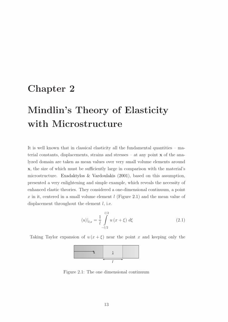
enhanced elastic theories. They considered a one-dimensional continuum, a point
x in it, centered in a small volume element l (Figure 2.1) and the mean value of
displacement throughout the element l, i.e.
〈u〉|l;x =1
l
l/2∫
−l/2
u (x+ ξ) dξ (2.1)
Taking Taylor expansion of u (x+ ξ) near the point x and keeping only the
Figure 2.1: The one dimensional continuum
13
Page 34
2. MINDLIN’S THEORY OF ELASTICITY WITH
MICROSTRUCTURE
constant term u (x+ ξ) one easily obtains from (2.1) that
〈u〉|l;x = u (x) (2.2)
which means that for constantly varying displacements in l, the aforementioned
assumption of classical elasticity is fulfilled. The same happens when the linear
term of Taylor’s expansion is also kept, i.e.
(x+ ξ) = u (x) + u′ (x) ξ ⇒ 〈u〉|l;x = u (x) (2.3)
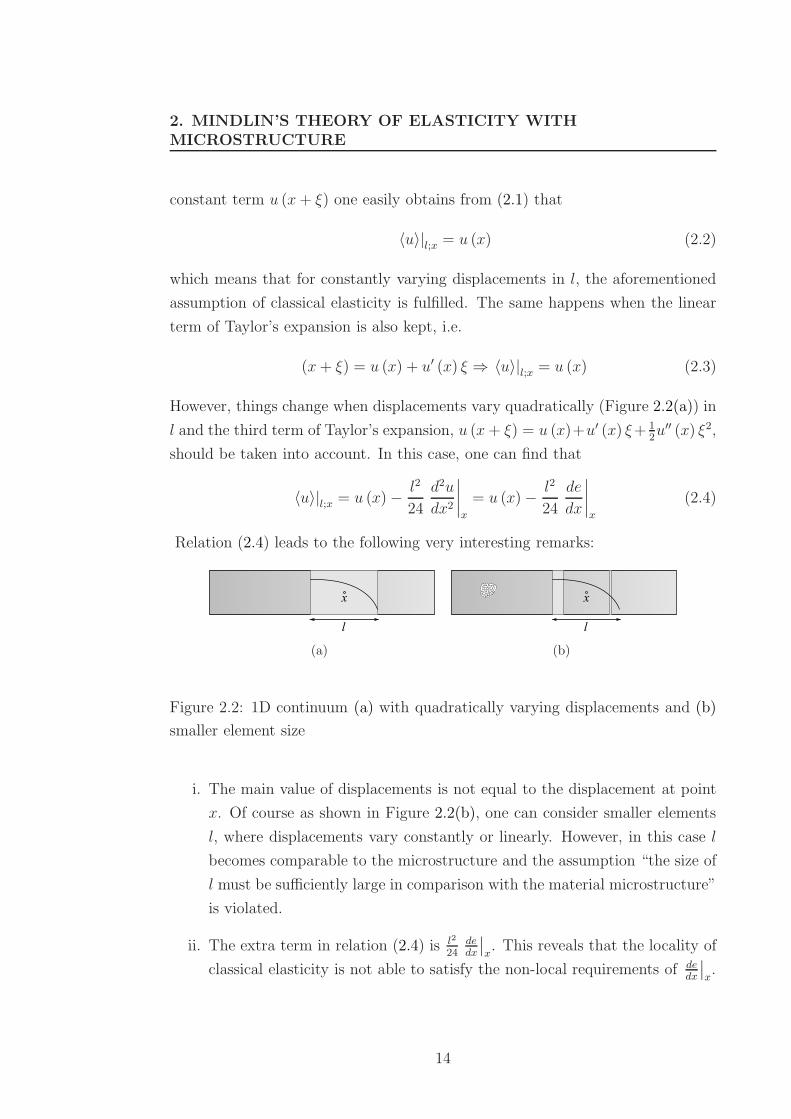
However, things change when displacements vary quadratically (Figure 2.2(a)) in
l and the third term of Taylor’s expansion, u (x+ ξ) = u (x)+u′ (x) ξ+ 12u′′ (x) ξ2,
should be taken into account. In this case, one can find that
〈u〉|l;x = u (x) − l2
24
d2u
dx2
∣
∣
∣
∣
x
= u (x) − l2
24
de
dx
∣
∣
∣
∣
x
(2.4)
Relation (2.4) leads to the following very interesting remarks:
(a) (b)
Figure 2.2: 1D continuum (a) with quadratically varying displacements and (b)
smaller element size
i. The main value of displacements is not equal to the displacement at point
x. Of course as shown in Figure 2.2(b), one can consider smaller elements
l, where displacements vary constantly or linearly. However, in this case l
becomes comparable to the microstructure and the assumption “the size of
l must be sufficiently large in comparison with the material microstructure”
is violated.
ii. The extra term in relation (2.4) is l2
24dedx
∣
∣
x. This reveals that the locality of
classical elasticity is not able to satisfy the non-local requirements of dedx
∣
∣
x.
14
Page 35
2.1 General Strain Gradient Theory of Elasticity
iii. The term l2
24dedx
∣
∣
xindicates that the problem can be solved if one formulates
a new theory of elasticity where higher order gradients of strains are taken
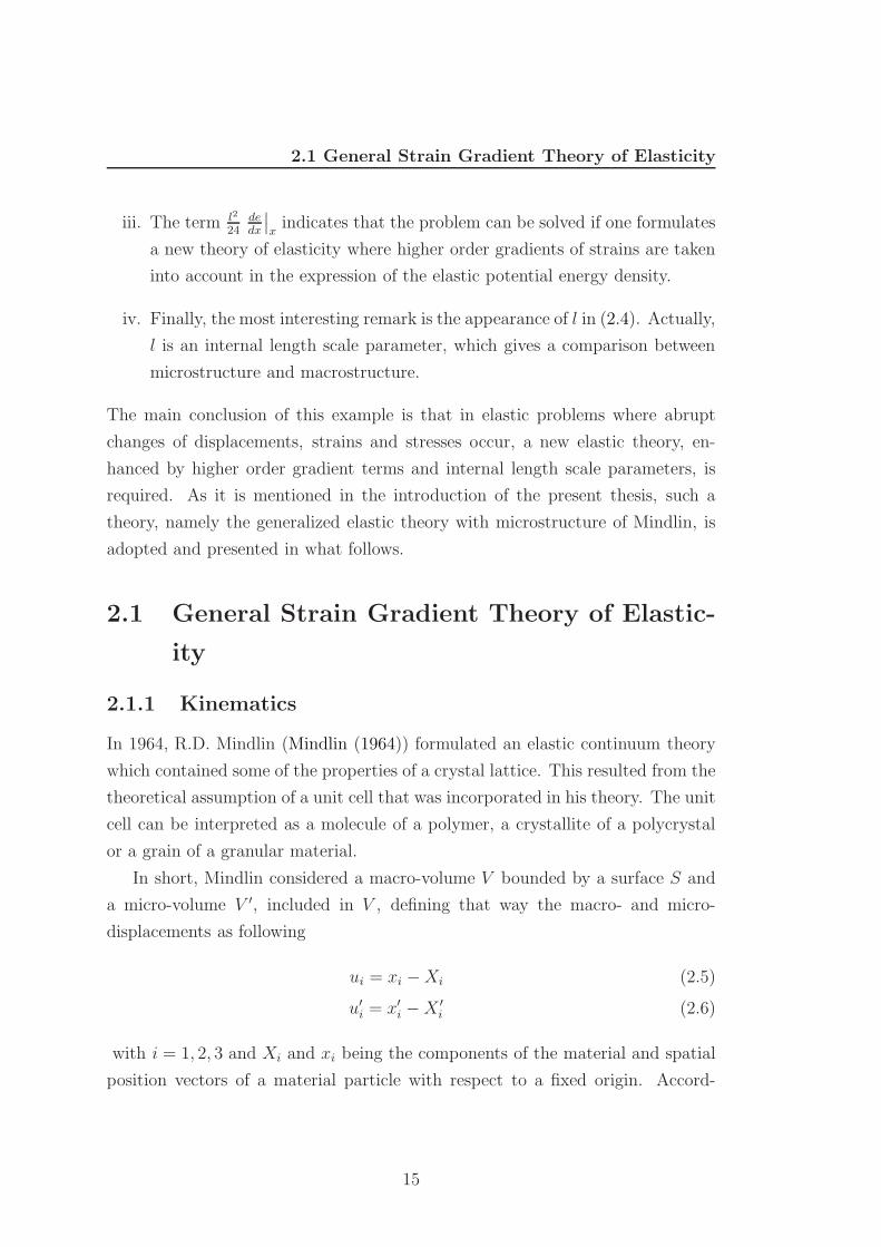
into account in the expression of the elastic potential energy density.
iv. Finally, the most interesting remark is the appearance of l in (2.4). Actually,
l is an internal length scale parameter, which gives a comparison between
microstructure and macrostructure.
The main conclusion of this example is that in elastic problems where abrupt
changes of displacements, strains and stresses occur, a new elastic theory, en-
hanced by higher order gradient terms and internal length scale parameters, is
required. As it is mentioned in the introduction of the present thesis, such a
theory, namely the generalized elastic theory with microstructure of Mindlin, is
adopted and presented in what follows.
2.1 General Strain Gradient Theory of Elastic-
ity
2.1.1 Kinematics
In 1964, R.D. Mindlin (Mindlin (1964)) formulated an elastic continuum theory
which contained some of the properties of a crystal lattice. This resulted from the
theoretical assumption of a unit cell that was incorporated in his theory. The unit
cell can be interpreted as a molecule of a polymer, a crystallite of a polycrystal
or a grain of a granular material.
In short, Mindlin considered a macro-volume V bounded by a surface S and
a micro-volume V ′, included in V , defining that way the macro- and micro-
displacements as following
ui = xi −Xi (2.5)
u′i = x′i −X ′i (2.6)
with i = 1, 2, 3 and Xi and xi being the components of the material and spatial
position vectors of a material particle with respect to a fixed origin. Accord-
15
Page 36
2. MINDLIN’S THEORY OF ELASTICITY WITH
MICROSTRUCTURE
ingly, X ′i and x′i are the material and spatial position vectors with respect to a
rectangular coordinate system that has its origin fixed in the particle.
Then, after the macro- and micro-displacements have been defined, he re-
quired that their gradients be small (|∂ui/∂Xi| ≈ |∂ui/∂xi| ≪ 1, |∂u′i/∂X ′i| ≈
|∂u′i/∂x′i| ≪ 1), which resulted to
∂uj
∂Xi≈ ∂uj
∂xi= ∂iuj (2.7)
∂u′j∂X ′
i
≈∂u′j∂x′i
= ∂′iu′j (2.8)
Furthermore, assuming that the micro-displacements can be expressed as a
sum of products of functions of x′i and other functions of xi and t (time), he wrote
the micro-displacement as an approximation, retaining only a single, linear term
of the series
u′j = x′kψkj (2.9)
The function ψkj is the micro-deformation. Differentiating the above equation
to obtain the displacement gradient results to
∂′iu′j = ψij (2.10)
which can be interpreted as the micro-deformation ψij being homogeneous in the
micro-volume V ′ and non-homogeneous in the macro-volume V .
The tensor ψij can be split into symmetric and antisymmetric parts, defining
that way the micro-strain ψ(ij) and the micro-rotation ψ[ij] respectively.
In addition, the macro-strain and macro-rotation tensors can be defined as in
classical elasticity,
ǫij =1
2(∂iuj + ∂jui) (2.11)
ωij =1
2(∂iuj − ∂jui) (2.12)
and the relative deformation (the difference of the macro-displacement gradient
and the micro-deformation) can be defined.
γij = ∂iuj − ψij (2.13)
16
Page 37
2.1 General Strain Gradient Theory of Elasticity
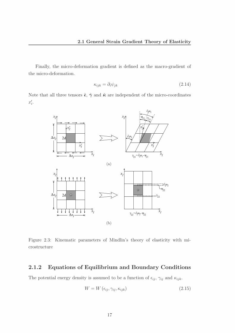
Finally, the micro-deformation gradient is defined as the macro-gradient of
the micro-deformation.
κijk = ∂iψjk (2.14)
Note that all three tensors ǫ, γ and κ are independent of the micro-coordinates
x′i.
(a)
(b)
Figure 2.3: Kinematic parameters of Mindlin’s theory of elasticity with mi-
crostructure
2.1.2 Equations of Equilibrium and Boundary Conditions
The potential energy density is assumed to be a function of ǫij , γij and κijk.
W = W (ǫij , γij, κijk) (2.15)
17
Page 38
2. MINDLIN’S THEORY OF ELASTICITY WITH
MICROSTRUCTURE
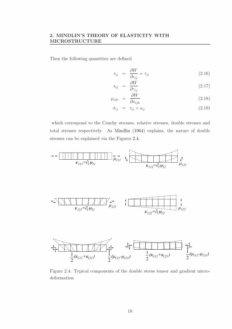
Then the following quantities are defined
τij =∂W
∂ǫij= τji (2.16)
sij =∂W
∂γij(2.17)
µijk =∂W
∂κijk(2.18)
σij = τij + sij (2.19)
which correspond to the Cauchy stresses, relative stresses, double stresses and
total stresses respectively. As Mindlin (1964) explains, the nature of double
stresses can be explained via the Figures 2.4.
Figure 2.4: Typical components of the double stress tensor and gradient micro-
deformation
18
Page 39
2.1 General Strain Gradient Theory of Elasticity
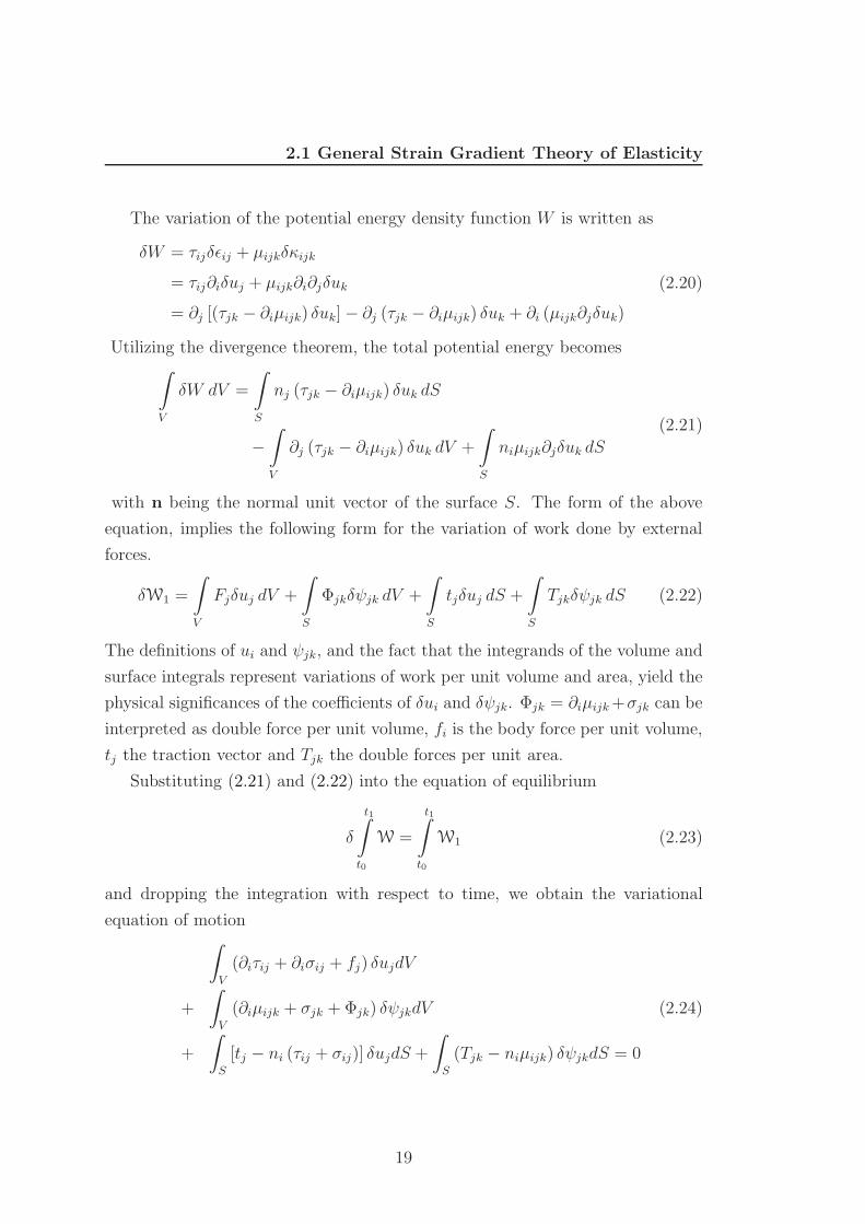
The variation of the potential energy density function W is written as
δW = τijδǫij + µijkδκijk
= τij∂iδuj + µijk∂i∂jδuk
= ∂j [(τjk − ∂iµijk) δuk] − ∂j (τjk − ∂iµijk) δuk + ∂i (µijk∂jδuk)
(2.20)
Utilizing the divergence theorem, the total potential energy becomes∫
V
δW dV =
∫
S
nj (τjk − ∂iµijk) δuk dS
−∫
V
∂j (τjk − ∂iµijk) δuk dV +
∫
S
niµijk∂jδuk dS
(2.21)
with n being the normal unit vector of the surface S. The form of the above
equation, implies the following form for the variation of work done by external
forces.
δW1 =
∫
V
Fjδuj dV +
∫
S
Φjkδψjk dV +
∫
S
tjδuj dS +
∫
S
Tjkδψjk dS (2.22)
The definitions of ui and ψjk, and the fact that the integrands of the volume and
surface integrals represent variations of work per unit volume and area, yield the
physical significances of the coefficients of δui and δψjk. Φjk = ∂iµijk +σjk can be
interpreted as double force per unit volume, fi is the body force per unit volume,
tj the traction vector and Tjk the double forces per unit area.
Substituting (2.21) and (2.22) into the equation of equilibrium
δ
t1∫
t0
W =
t1∫
t0
W1 (2.23)
and dropping the integration with respect to time, we obtain the variational
equation of motion∫
V
(∂iτij + ∂iσij + fj) δujdV
+
∫
V
(∂iµijk + σjk + Φjk) δψjkdV (2.24)
+
∫
S
[tj − ni (τij + σij)] δujdS +
∫
S
(Tjk − niµijk) δψjkdS = 0
19
Page 40
2. MINDLIN’S THEORY OF ELASTICITY WITH
MICROSTRUCTURE
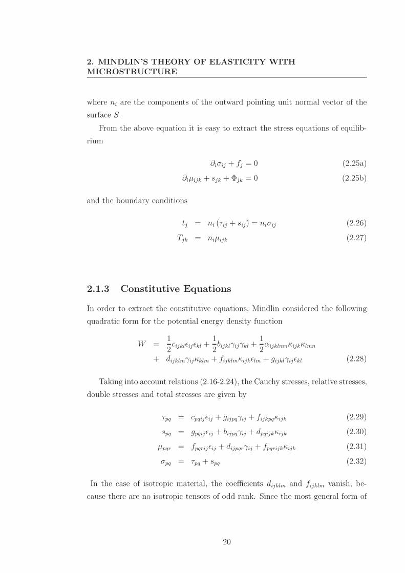
where ni are the components of the outward pointing unit normal vector of the
surface S.
From the above equation it is easy to extract the stress equations of equilib-
rium
∂iσij + fj = 0 (2.25a)
∂iµijk + sjk + Φjk = 0 (2.25b)
and the boundary conditions
tj = ni (τij + sij) = niσij (2.26)
Tjk = niµijk (2.27)
2.1.3 Constitutive Equations
In order to extract the constitutive equations, Mindlin considered the following
quadratic form for the potential energy density function
W =1
2cijklǫijǫkl +
1
2bijklγijγkl +
1
2αijklmnκijkκlmn
+ dijklmγijκklm + fijklmκijkǫlm + gijklγijǫkl (2.28)
Taking into account relations (2.16-2.24), the Cauchy stresses, relative stresses,
double stresses and total stresses are given by
τpq = cpqijǫij + gijpqγij + fijkpqκijk (2.29)
spq = gpqijǫij + bijpqγij + dpqijkκijk (2.30)
µpqr = fpqrijǫij + dijpqrγij + fpqrijkκijk (2.31)
σpq = τpq + spq (2.32)
In the case of isotropic material, the coefficients dijklm and fijklm vanish, be-
cause there are no isotropic tensors of odd rank. Since the most general form of
20
Page 41
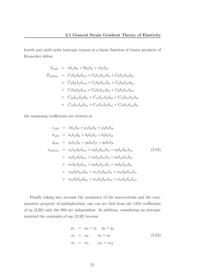
2.1 General Strain Gradient Theory of Elasticity
fourth and sixth order isotropic tensors is a linear function of tensor products of
Kronecker deltas
Lijkl = aδijδkl + bδikδjl + cδilδjk
Fijklmn = C1δijδklδmn + C2δijδkmδln + C3δijδknδlm
+ C4δikδjlδmn + C5δikδjmδln + C6δikδjnδlm
+ C7δilδjkδmn + C8δilδjmδkn + C9δilδjnδkm
+ C10δimδjkδln + C11δimδjlδkn + C12δimδjnδkl
+ C13δinδjkδlm + C14δinδjlδkm + C15δinδjmδkl
the remaining coefficients are written as
cijkl = λδijδkl + µ1δikδjl + µ2δilδjk
bijkl = b1δijδkl + b2δikδjl + b3δilδjk
gijkl = g1δijδkl + g2δikδjl + g3δilδjk
aijklmn = a1δijδklδmn + a2δijδkmδnl + a3δijδknδlm (2.33)
+ a4δjkδilδmn + a5δjkδimδnl + a6δjkδinδlm
+ a7δkiδjlδmn + a8δkiδjmδnl + a9δkiδjnδlm
+ a10δilδjmδkn + a11δjlδkmδin + a12δklδimδjn
+ a13δilδjnδkm + a14δjlδknδim + a15δklδinδjm
Finally taking into account the symmetry of the macro-strain and the com-
mutative property of multiplication, one can see that from the 1458 coefficients
of eq (2.28) only the 903 are independent. In addition, considering an isotropic
material the constants of eqs (2.33) become
µ1 = µ2 = µ, g2 = g3
a1 = a6, a2 = a9 (2.34)
a5 = a7, a11 = a12
21
Page 42
2. MINDLIN’S THEORY OF ELASTICITY WITH
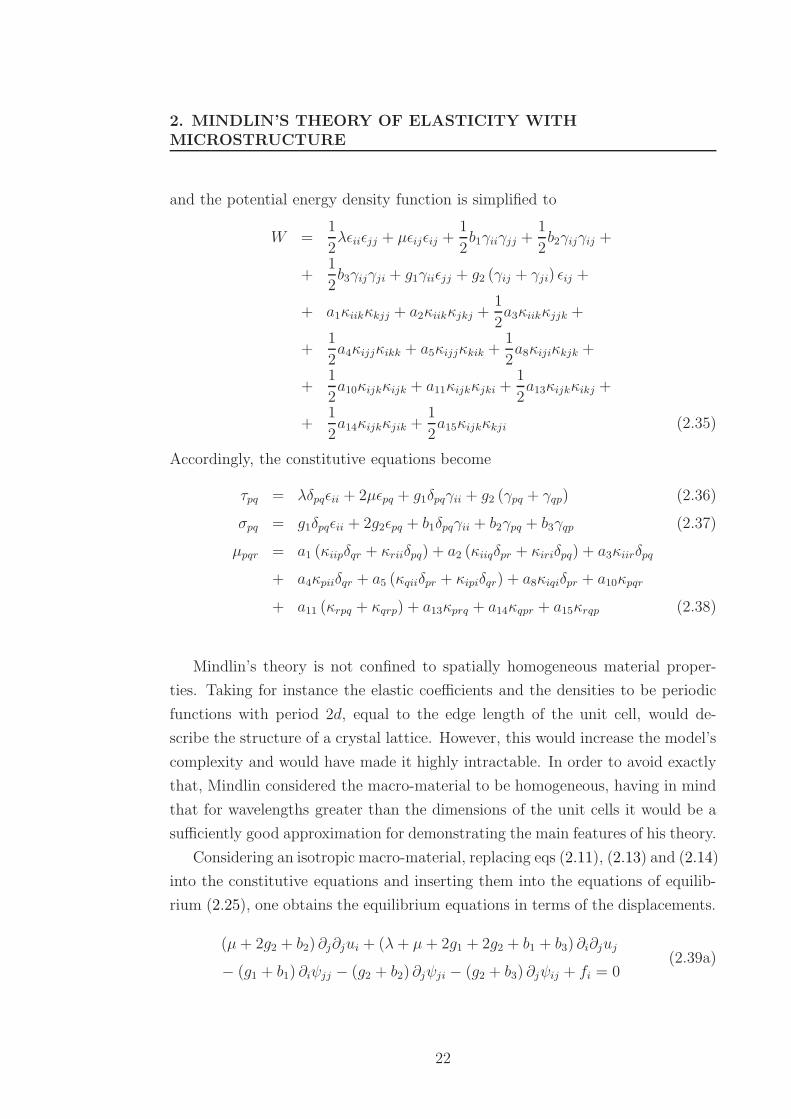
MICROSTRUCTURE
and the potential energy density function is simplified to
W =1
2λǫiiǫjj + µǫijǫij +
1
2b1γiiγjj +
1
2b2γijγij +
+1
2b3γijγji + g1γiiǫjj + g2 (γij + γji) ǫij +
+ a1κiikκkjj + a2κiikκjkj +1
2a3κiikκjjk +
+1
2a4κijjκikk + a5κijjκkik +
1
2a8κijiκkjk +
+1
2a10κijkκijk + a11κijkκjki +
1
2a13κijkκikj +
+1
2a14κijkκjik +
1
2a15κijkκkji (2.35)
Accordingly, the constitutive equations become
τpq = λδpqǫii + 2µǫpq + g1δpqγii + g2 (γpq + γqp) (2.36)
σpq = g1δpqǫii + 2g2ǫpq + b1δpqγii + b2γpq + b3γqp (2.37)
µpqr = a1 (κiipδqr + κriiδpq) + a2 (κiiqδpr + κiriδpq) + a3κiirδpq
+ a4κpiiδqr + a5 (κqiiδpr + κipiδqr) + a8κiqiδpr + a10κpqr
+ a11 (κrpq + κqrp) + a13κprq + a14κqpr + a15κrqp (2.38)
Mindlin’s theory is not confined to spatially homogeneous material proper-
ties. Taking for instance the elastic coefficients and the densities to be periodic
functions with period 2d, equal to the edge length of the unit cell, would de-
scribe the structure of a crystal lattice. However, this would increase the model’s
complexity and would have made it highly intractable. In order to avoid exactly
that, Mindlin considered the macro-material to be homogeneous, having in mind
that for wavelengths greater than the dimensions of the unit cells it would be a
sufficiently good approximation for demonstrating the main features of his theory.
Considering an isotropic macro-material, replacing eqs (2.11), (2.13) and (2.14)
into the constitutive equations and inserting them into the equations of equilib-
rium (2.25), one obtains the equilibrium equations in terms of the displacements.
(µ+ 2g2 + b2) ∂j∂jui + (λ+ µ+ 2g1 + 2g2 + b1 + b3) ∂i∂juj
− (g1 + b1) ∂iψjj − (g2 + b2) ∂jψji − (g2 + b3) ∂jψij + fi = 0(2.39a)
22
Page 43
2.2 Form I, II and III Gradient Elasticity Theories
(a1 + a5) (∂k∂lψklδij + ∂i∂jψkk) + (a2 + a11) (∂j∂kψki + ∂i∂kψjk)
+ (a13 + a14) ∂i∂kψkj + a4∂k∂kψllδij + (a8 + a15) ∂j∂kψik
+ a10∂k∂kψij + a13∂k∂kψji + g1∂kukδij + g2 (∂iuj + ∂jui)
+ b1 (∂kuk − ψkk) δij + b2 (∂iuj − ψij) + b3 (∂jui − ψji) + Φij = 0
(2.39b)
2.2 Simplified Versions of Mindlin’s General The-
ory: Form I, II and III Gradient Elasticity
Theories
Mindlin found that the modes that appear in a gradient elastic material due to
a micro-vibration, ψij = Aijeiωt, (dilatational, shear, equivoluminal extensional
and rotational), are analogous to the thickness modes of vibration that appear
in homogeneous plates. Having in mind the derivation of the low frequency
approximation in plate theory, he used the same process to simplify his gradient
elasticity theory.
In homogeneous plates, when the excited frequencies are low compared to the
thickness modes of the plate and the wavelengths long compared to the thickness
of the plate, the coupling of the flexural and extensional modes with the thickness
modes is negligible. As the frequencies of the flexural and extensional modes
approach zero, the thickness-shear deformation approaches zero, but the thickness
stretch deformation does not. However, the stress associated to the thickness
stretch tends to zero. This means that the symmetric and anti-symmetric parts
of deformation and stress have to be treated differently when deriving the low
frequency approximation.
To obtain the low frequency approximation for flexure in plate theory, the
thickness shear deformation is sent to zero and the associated modulus of elasticity
is sent to infinity. Furthermore, in the case of extension, the thickness stress is
set equal to zero and the resulting constitutive equation is used to eliminate
the thickness strain from the remaining equations. In both cases, flexure and
extension, the thickness velocities are set equal to zero in the kinetic energy,
because their contribution is negligible.
23
Page 44
2. MINDLIN’S THEORY OF ELASTICITY WITH
MICROSTRUCTURE
As mentioned earlier, the modes appearing in gradient elasticity can be as-
sociated with the ones appearing in homogeneous plate theory. Specifically, the
micro-modes are analogous to the thickness modes of vibration and the trans-
verse and longitudinal acoustic modes are analogous to the flexural and exten-
sional modes of the plate. Furthermore, the micro-velocities ψij correspond to the
thickness velocities of the plate and the dimensions of the unit cell 2d are similar
to the plate thickness. Finally, the antisymmetric part of the relative deformation
γ[ij] is analogous to the thickness shear deformation, the coefficients b2 and b3 of
eq. (2.35) correspond to the thickness shear moduli and the symmetric part of
the relative stress s(ij) is associated with the stress resulting from the thickness
stretch of the plate.
Using the above analogies, the assumptions for the derivation of the low fre-
quency approximation in plate theory can be translated in terms of gradient
elasticity.
s(ij) = 0 (2.40)
γ[ij] → 0 (2.41)
b2 − b3 → 0 (2.42)
These assumptions form the basic hypothesis for the low frequency approximation
of Mindlin’s theory. Obviously all the above are also valid for static problems.
The constitutive equations for the Cauchy and relative stresses (2.36-2.38)
become
τpq = λδpqǫii + 2µǫpq + g1δpqγii + 2g2γpq (2.43)
s(pq) = g1δpqǫii + 2g2ǫpq + b1δpqγii + (b2 + b3) γ(pq) (2.44)
s[pq] = (b2 − b3) γ[pq] (2.45)
Equation (2.44) can now be solved for γ(pq)
γ(pq) = −αδpqǫii + (1 − β) ǫpq (2.46)
with α and β depending on the potential energy density function coefficients.
α =1
b2 + b3
(
g1 −b1 (3g1 + 2g2)
3b1 + b2 + b3
)
β = 1 +2g2
b2 + b3
24
Page 45
2.2 Form I, II and III Gradient Elasticity Theories
Since γ[pq] has been sent to zero, the symmetric and antisymmetric parts of
the micro-deformation are functions of the macro-strains and the macro-rotations
respectively.
ψ(pq) = αδpqǫii + βǫpq (2.47a)
ψ[pq] = ωpq (2.47b)
Accordingly the micro-deformations κijk become
κijk → ακillδjk +1
2(1 + β) κijk −
1
2(1 − β) κikj (2.48)
with κijk = ∂i∂juk = κjik. This means that in static problems, κijk becomes κijk,
a function of the second gradient of displacements. Then the potential energy
density function is written
W → W =1
2λǫiiǫjj + µǫijǫij + α1κiikκkjj
+ α2κijjκikk + α3κiikκjjk + α4κijkκijk + α5κijkκkji
(2.49)
with the constants λ, µ and α1-α5 depending on the potential energy density
function coefficients as shown in Appendix A. This is the first form for the
potential energy density function, also referred to as Form I.
The components κijk may be arranged in tensors, whose components are inde-
pendent linear combinations of ∂i∂juk in more than one ways, resulting in different
forms of he potential energy density function. Specifically, arranging the terms
in such a way that the gradient of strain is formed, leads to the second form of
Mindlin’s gradient elasticity theory.
κijk ≡ ∂iǫjk =1
2(∂i∂juk + ∂i∂kuj) = κikj (2.50)
Then, the potential energy density becomes
W → W =1
2λǫiiǫjj + µǫijǫij + α1κiikκkjj
+ α2κijjκikk + α3κiikκjjk + α4κijkκijk + α5κijkκkji
(2.51)
with λ = λ, µ = µ and α1-α5 presented in Appendix A. This form is refereed to
as Form II.
25
Page 46
2. MINDLIN’S THEORY OF ELASTICITY WITH
MICROSTRUCTURE
Finally, separating the curl of the strain κij from the second gradient of dis-
placements results to the third form, which is refereed to as Form III.
κij ≡ ejlm∂lǫmi =1
2ejlm∂i∂lum (2.52)
¯κijk = κijk +1
3eiljκkl +
1
3eilkκjl =
1
3(∂i∂juk + ∂k∂iuj + ∂j∂kui) (2.53)
κijk = ¯κijk −1
3eilj κkl −
1
3eilkκjl (2.54)
The potential energy density expression for Form III is now expressed as a
function of κij and ¯κijk.
W → W =1
2λǫiiǫjj + µǫijǫij + 2d1κijκij + 2d2κijκji
+3
2α1 ¯κiij ¯κkkj + α2 ¯κijk ¯κijk + f eijkκij ¯κkll
(2.55)
with the constants d1, d2, α1, α2 and f presented in Appendix A.
2.3 Form II Gradient Elasticity Theory
In this section the equilibrium equations corresponding to Mindlin’s Form II
gradient elasticity theory are derived.
As mentioned earlier, the potential energy density function W of the gen-
eral gradient elasticity theory becomes W in the case of the Form II, when the
components ∂i∂juk are arranged in such a way that the gradient of strains is
formed.
W =1
2λǫiiǫjj + µǫijǫij + α1κiikκkjj
+ α2κijjκikk + α3κiikκjjk + α4κijkκijk + α5κijkκkji
(2.56)
The stresses are now defined with respect to W as
τij =∂W
∂ǫij= τji (2.57a)
µijk =∂W
∂κijk= µikj (2.57b)
26
Page 47
2.3 Form II Gradient Elasticity Theory
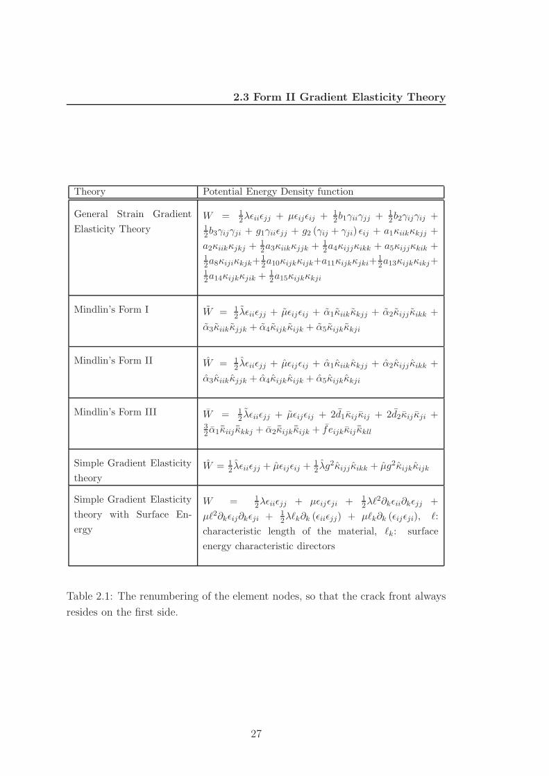
Theory Potential Energy Density function
General Strain Gradient
Elasticity Theory
W = 12λǫiiǫjj + µǫijǫij + 1
2b1γiiγjj + 12b2γijγij +
12b3γijγji + g1γiiǫjj + g2 (γij + γji) ǫij + a1κiikκkjj +
a2κiikκjkj + 12a3κiikκjjk + 1
2a4κijjκikk + a5κijjκkik +12a8κijiκkjk+
12a10κijkκijk+a11κijkκjki+
12a13κijkκikj+
12a14κijkκjik + 1
2a15κijkκkji
Mindlin’s Form I W = 12 λǫiiǫjj + µǫijǫij + α1κiikκkjj + α2κijj κikk +
α3κiikκjjk + α4κijkκijk + α5κijkκkji
Mindlin’s Form II W = 12 λǫiiǫjj + µǫijǫij + α1κiikκkjj + α2κijj κikk +
α3κiikκjjk + α4κijkκijk + α5κijkκkji
Mindlin’s Form III W = 12 λǫiiǫjj + µǫijǫij + 2d1κij κij + 2d2κij κji +
32 α1 ¯κiij ¯κkkj + α2 ¯κijk ¯κijk + f eijkκij ¯κkll
Simple Gradient Elasticity
theoryW = 1
2 λǫiiǫjj + µǫijǫij + 12 λg2κijjκikk + µg2κijkκijk
Simple Gradient Elasticity
theory with Surface En-
ergy
W = 12λǫiiǫjj + µǫijǫji + 1
2λℓ2∂kǫii∂kǫjj +
µℓ2∂kǫij∂kǫji + 12λℓk∂k (ǫiiǫjj) + µℓk∂k (ǫijǫji), ℓ:
characteristic length of the material, ℓk: surface
energy characteristic directors
Table 2.1: The renumbering of the element nodes, so that the crack front always
resides on the first side.
27
Page 48
2. MINDLIN’S THEORY OF ELASTICITY WITH
MICROSTRUCTURE
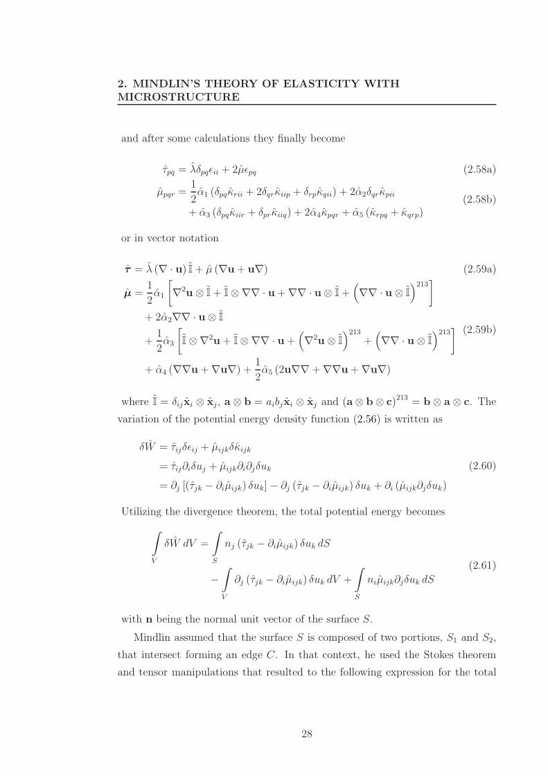
and after some calculations they finally become
τpq = λδpqǫii + 2µǫpq (2.58a)
µpqr =1
2α1 (δpqκrii + 2δqrκiip + δrpκqii) + 2α2δqrκpii
+ α3 (δpqκiir + δprκiiq) + 2α4κpqr + α5 (κrpq + κqrp)(2.58b)
or in vector notation
τ = λ (∇ · u) I + µ (∇u + u∇) (2.59a)
µ =1
2α1
[
∇2u ⊗ I + I ⊗∇∇ · u + ∇∇ · u⊗ I +(
∇∇ · u ⊗ I
)213]
+ 2α2∇∇ · u⊗ I
+1
2α3
[
I ⊗∇2u + I ⊗∇∇ · u +(
∇2u ⊗ I
)213
+(
∇∇ · u ⊗ I
)213]
+ α4 (∇∇u + ∇u∇) +1
2α5 (2u∇∇ + ∇∇u + ∇u∇)
(2.59b)
where I = δijxi ⊗ xj, a ⊗ b = aibjxi ⊗ xj and (a⊗ b ⊗ c)213 = b ⊗ a ⊗ c. The
variation of the potential energy density function (2.56) is written as
δW = τijδǫij + µijkδκijk
= τij∂iδuj + µijk∂i∂jδuk
= ∂j [(τjk − ∂iµijk) δuk] − ∂j (τjk − ∂iµijk) δuk + ∂i (µijk∂jδuk)
(2.60)
Utilizing the divergence theorem, the total potential energy becomes
∫
V
δW dV =
∫
S
nj (τjk − ∂iµijk) δuk dS
−∫
V
∂j (τjk − ∂iµijk) δuk dV +
∫
S
niµijk∂jδuk dS
(2.61)
with n being the normal unit vector of the surface S.
Mindlin assumed that the surface S is composed of two portions, S1 and S2,
that intersect forming an edge C. In that context, he used the Stokes theorem
and tensor manipulations that resulted to the following expression for the total
28
Page 49
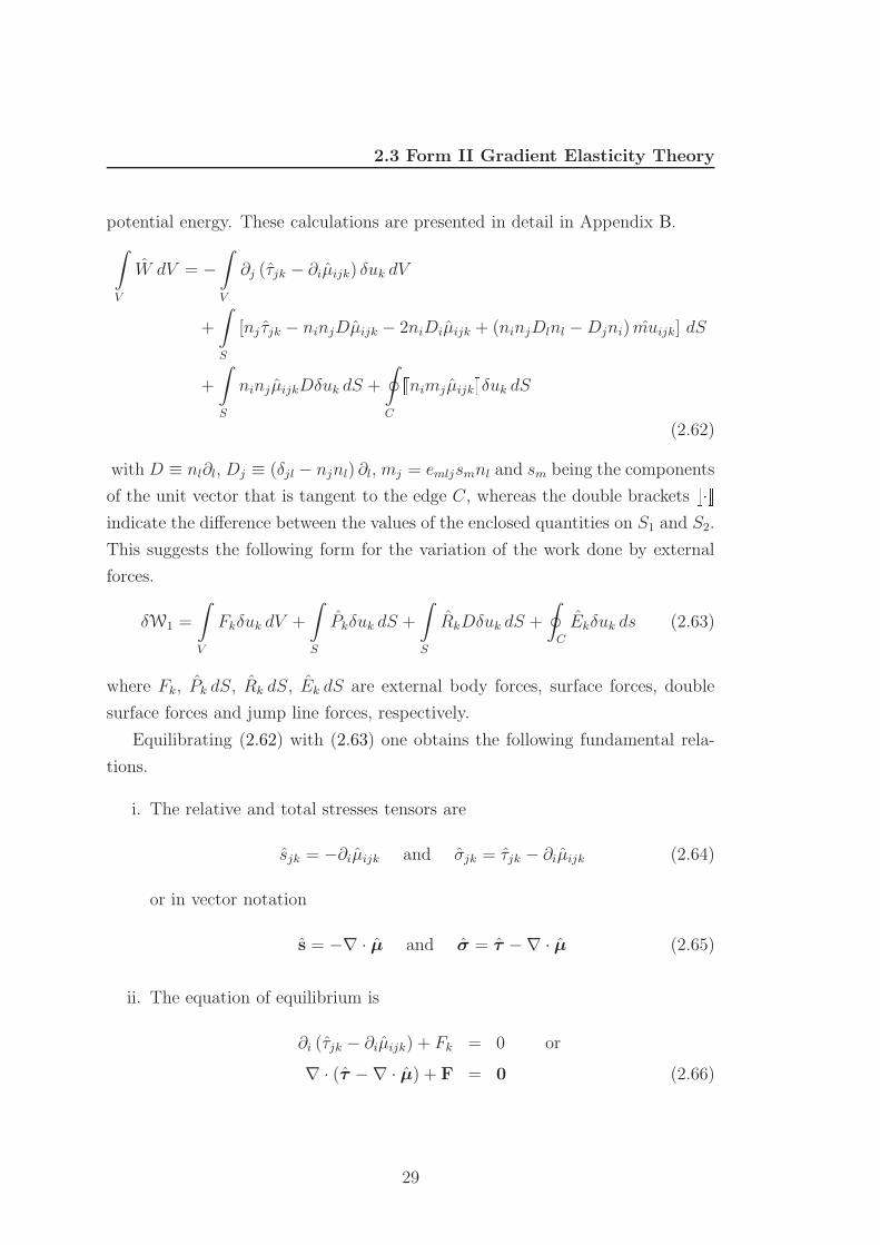
2.3 Form II Gradient Elasticity Theory
potential energy. These calculations are presented in detail in Appendix B.
∫
V
W dV = −∫
V
∂j (τjk − ∂iµijk) δuk dV
+
∫
S
[nj τjk − ninjDµijk − 2niDiµijk + (ninjDlnl −Djni) muijk] dS
+
∫
S
ninjµijkDδuk dS +
∮
C
JnimjµijkKδuk dS
(2.62)
with D ≡ nl∂l, Dj ≡ (δjl − njnl) ∂l, mj = emljsmnl and sm being the components
of the unit vector that is tangent to the edge C, whereas the double brackets J·Kindicate the difference between the values of the enclosed quantities on S1 and S2.
This suggests the following form for the variation of the work done by external
forces.
δW1 =
∫
V
Fkδuk dV +
∫
S
Pkδuk dS +
∫
S
RkDδuk dS +
∮
C
Ekδuk ds (2.63)
where Fk, Pk dS, Rk dS, Ek dS are external body forces, surface forces, double
surface forces and jump line forces, respectively.
Equilibrating (2.62) with (2.63) one obtains the following fundamental rela-
tions.
i. The relative and total stresses tensors are
sjk = −∂iµijk and σjk = τjk − ∂iµijk (2.64)
or in vector notation
s = −∇ · µ and σ = τ −∇ · µ (2.65)
ii. The equation of equilibrium is
∂i (τjk − ∂iµijk) + Fk = 0 or
∇ · (τ −∇ · µ) + F = 0 (2.66)
29
Page 50
2. MINDLIN’S THEORY OF ELASTICITY WITH
MICROSTRUCTURE
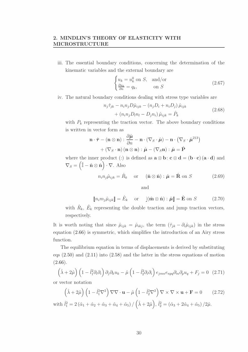
iii. The essential boundary conditions, concerning the determination of the
kinematic variables and the external boundary are{
uk = u0k on S, and/or
∂uk
∂n= qk, on S
(2.67)
iv. The natural boundary conditions dealing with stress type variables are
nj τjk − ninjDµijk − (njDi + niDj) µijk
+ (ninjDlnl −Djni) µijk = Pk
(2.68)
with Pk representing the traction vector. The above boundary conditions
is written in vector form as
n · τ − (n ⊗ n) :∂µ
∂n− n · (∇S · µ) − n ·
(
∇S · µ213)
+ (∇S · n) (n⊗ n) : µ− (∇Sn) : µ = P
where the inner product (:) is defined as a ⊗ b : c ⊗ d = (b · c) (a · d) and
∇S =(
I − n⊗ n)
· ∇. Also
ninjµijk = Rk or (n⊗ n) : µ = R on S (2.69)
andJnimjµijkK = Ek or J(m⊗ n) : µK = E on S (2.70)
with Rk, Ek representing the double traction and jump traction vectors,
respectively.
It is worth noting that since µijk = µikj, the term (τjk − ∂iµijk) in the stress
equation (2.66) is symmetric, which simplifies the introduction of an Airy stress
function.
The equilibrium equation in terms of displacements is derived by substituting
eqs (2.50) and (2.11) into (2.58) and the latter in the stress equations of motion
(2.66).(
λ+ 2µ)(
1 − l21∂i∂i
)
∂j∂kuk − µ(
1 − l22∂i∂i
)
ejmnenpq∂m∂puq + Fj = 0 (2.71)
or vector notation(
λ+ 2µ)(
1 − l21∇2)
∇∇ · u − µ(
1 − l22∇2)
∇×∇× u + F = 0 (2.72)
with l21 = 2 (α1 + α2 + α3 + α4 + α5) /(
λ+ 2µ)
, l22 = (α3 + 2α4 + α5) /2µ.
30
Page 51
2.4 Integral Representation of the Form II Gradient Elastic Problem
2.4 Integral Representation of the Form II Gra-
dient Elastic Problem
2.4.1 Reciprocal Integral Identity
In the previous section, the tilde (·) has been used to describe the fields related
to the Form I gradient elasticity theory, in accordance to Mindlin (1964). From
now on, the tilde (·) will be used over a symbol to specify that it is a tensor of
second or higher order.
In order to proceed with the integral representation of a static Form II gra-
dient elastic problem, a reciprocal integral identity must be derived, analogous
to Betti’s reciprocal identity for the classical elasticity (Brebbia & Dominguez
(1992)).
Consider a gradient elastic material with volume V and surrounding surface
S. Also consider two different deformation states for this material, denoted as
(u, σ) and (u∗, σ∗) with u, u∗ being the displacement vectors and σ, σ∗ being
the total stress tensors of the first and second deformation state respectively.
Betti’s theorem for classical elasticity states that the work done by the external
forces of the first state in the displacements of the second state is equal to the
work of the external forces of the second state in the displacements of the first
state. In order to derive an identity analogous to Betti’s the same procedure as
followed by Polyzos et al. (2003) is applied.
First, a vector w involving the two deformation states is defined.
w = σ · u∗ − σ∗ · u (2.73)
Replacing the total stresses from eq (2.65), calculating the divergence of w and
exploiting the identities ∇· (τ · u) = (∇ · τ ) ·u+ τ : ∇u and τ : ∇u− τ : ∇u = 0
yields
∇ ·w = ∇ · (τ −∇µ) · u∗ − [∇ · (τ ∗ −∇ · µ∗)] · u− (∇ · µ) : ∇u∗ + (∇ · µ∗) : ∇u
(2.74)
31
Page 52
2. MINDLIN’S THEORY OF ELASTICITY WITH
MICROSTRUCTURE
Now, applying the Gauss divergence theorem for w over the volume V produces
the following:∫
V
[∇ · (τ −∇ · µ)] · u∗ − [∇ · (τ ∗ −∇ · µ∗)] · u dV
−∫
V
(∇ · µ) : ∇u∗ − (∇ · µ∗) : ∇u dV
=
∫
S
[n · (τ −∇ · µ)] · u∗ − [n · (τ ∗ −∇ · µ∗)] · u dS
(2.75)
Using the equilibrium equation (eq (2.66)) for both deformation states with forces
f and f∗ respectively, the above integral equation becomes:∫
V
f∗ · u − f · u∗ dV
+
∫
V
(∇ · µ∗) : ∇u− (∇ · µ) : ∇u∗ dV =
∫
S
t · u∗ − t∗ · u dS(2.76)
with t = n · (τ −∇ · µ) and t∗ = n · (τ ∗ −∇ · µ∗) being the traction vectors for
the two states, acting on the boundary surface S.
Furthermore, using eq (2.65) and Green’s integral identity, the second volume
integral of the above equation can be written as a surface integral over S (Polyzos
et al. (2003)).
∫
V
(∇ · µ∗) : ∇u−(∇ · µ) : ∇u∗ dV =
∫
S
(n · µ∗) : ∇u−(n · µ) : ∇u∗ dS (2.77)
In view of the above, eq (2.76) becomes
∫
V
f∗ · u − f · u∗ dV
+
∫
S
(n · µ∗) : ∇u− (n · µ) : ∇u∗ dS =
∫
S
t · u∗ − t∗ · u dS(2.78)
Finally, using the identities
n · µ : ∇u∗ = (n · µ · n) (n · ∇u∗) + (n · µ) : ∇Su∗ (2.79)
32
Page 53
2.4 Integral Representation of the Form II Gradient Elastic Problem
(n · µ) : ∇Su = ∇S · [(n · µ) · u∗] −[
∇Sn : µ+ n ·(
∇S · µ213)]
· u∗ (2.80)
∇S · [(n · µ) · u∗] = n · ∇S × [n× (n · µ · u∗)] + [(∇S · n) (n⊗ n) : µ]u∗ (2.81)
the reciprocal integral identity becomes
∫
V
f∗ · u − f · u∗ dV +
∫
S
P∗ · u− P · u∗ dS
=
∫
S
R · ∂u∗
∂n− R∗ · ∂u
∂ndS +
∑
a
∮
Ca
E · u∗ − E∗ · u dC(2.82)
with
P = n · τ − (n⊗ n) :∂µ
∂n− n · (∇S · µ) − n ·
(
∇S · µ213)
+ (∇S · n) (n⊗ n) : µ− (∇Sn) : µ (2.83)
R = (n⊗ n) : µ (2.84)
E = J(m⊗ n) : µK (2.85)
and a being the total number of edges Ca of the surface S. It must be noted
here, that in the two dimensional case, the line integral of eq (2.82) reduces to a
sum of distinct values, over the corners of S. It should also be mentioned here
that Giannakopoulos et al. (2006) have also derived the same reciprocity relation
in their paper dealing with the Saint-Venant principle for linear strain-gradient
elastic bodies.
2.4.2 2D and 3D Fundamental Solutions
The fundamental displacement is defined as the displacement of point x due to
a unit excitation δ (x,y) I at point y. This means that the fundamental solution
u∗ (x,y) of the Form II gradient elasticity is a tensor satisfying the following
partial differential equation.
(
λ+ 2µ)(
1 − l21∇2)
∇∇·u∗ (r)−µ(
1 − l22∇2)
∇×∇×u∗ (r) = −δ (r) I (2.86)
with r = |x − y| and δ (r) being the Dirac delta function.
33
Page 54
2. MINDLIN’S THEORY OF ELASTICITY WITH
MICROSTRUCTURE
It is worth noting here, that using the identity ∇2 = ∇∇·+∇×∇× and after
some calculations we end up with a more familiar form of eq (2.86).
(
1 − l22∇2)
∆∗u∗ (r) +(
λ+ 2µ)(
l22 − l21
)
∇2∇ (∇ · u∗ (r)) = −δ (r) I (2.87)
with ∆∗ = µ∇2 +(
λ+ µ)
∇∇· being the differential operator of classical elas-
ticity.
The Dirac delta function in eq (2.86) may be replaced by the Laplacian of a
scalar function γ (r), which has the following form:
γ (r) =
{
12π
ln(
1r
)
, for 2D1
4πr, for 3D
(2.88)
since γ (r) is the fundamental solution of the Laplacian operator, i.e. ∇2γ (r) =
−δ (r).
Furthermore, Dassios & Lindell (2001) have proven that any second order
tensor can be decomposed in three parts. The first is the gradient of the gradient
of a scalar function φ (r), the second is the gradient of the curl of a vector function
A (r) and the last part is the curl of the curl of a dyadic function G (r).
u∗ (r) = ∇∇φ (r) + ∇∇× A (r) + ∇×∇× G (r) (2.89)
Utilizing the identity ∇2[
γ (r) I
]
= ∇∇ ·[
γ (r) I
]
− ∇ × ∇ ×[
γ (r) I
]
, and
replacing all the above in eq (2.86), the latter becomes
∇∇[(
λ+ 2µ)(
∇2φ (r) − l21∇4φ (r))]
+∇∇×[(
λ+ 2µ)(
∇2A (r) − l21∇4A (r))]
+∇×∇×[
µ(
∇2G (r) − l22∇4G (r))]
= ∇∇γ (r) I −∇×∇× γ (r) I
(2.90)
For the above equation to hold true each part of the left hand side must be
equated to the corresponding part on the right hand side.
(
λ+ 2µ)(
∇2φ (r) − l21∇4φ (r))
= γ (r) (2.91)(
λ+ 2µ)(
∇2A (r) − l21∇4A (r))
= 0 (2.92)
µ(
∇2G (r) − l22∇4G (r))
= −γ (r) I (2.93)
34
Page 55
2.4 Integral Representation of the Form II Gradient Elastic Problem
The radial nature of the fundamental solution exists only when A = 0. The
order of eqs (2.91) and (2.93) can be reduced by replacing f (r) = ∇2φ (r) and
g (r) = ∇2G respectively.(
λ+ 2µ)(
f (r) − l21∇2f (r))
= γ (r) (2.94)
µ(
g (r) − l22∇2g (r))
= −γ (r) I (2.95)
For the 3D case, the last two equations admit solutions of the form
f (r) = ∇2φ (r) =1
4π(
λ + 2µ)
(
1
r− e−r/l1
r
)
(2.96)
g (r) = ∇2G (r) = − 1
4πµ
(
1
r− e−r/l2
r
)
I (2.97)
which yield
φ (r) =1
4π(
λ+ 2µ)
(
r
2− l21r− l21
e−r/l1
r
)
(2.98)
G (r) = − 1
4πµ
(
r
2+l22r− l22
e−r/l2
r
)
I (2.99)
Accordingly for the 2D case, the corresponding functions φ (r) and G (r) are
found to be
φ (r) = − 1 − 2ν
4πµ (1 − ν)
[
r2
4(ln r − 1) + l21 ln r + l21K0
(
r
l1
)]
(2.100)
G (r) =1
2πµ
[
r2
4(ln r − 1) + l22 ln r + l22K0
(
r
l2
)]
I (2.101)
with 2ν = λ/(
λ+ µ)
and K0 (·) the modified Bessel function of the second kind
and zeroth order.
Substituting the above results for φ (r), A (r) and G (r), into the decomposed
expression for the displacement (eq (2.89)) we end up with the final form of the
displacement fundamental solution.
u∗ (r) =1
(a− 1) 8πµ (1 − ν)
[
Ψ (r) I −X (r) r ⊗ r]
(2.102)
35
Page 56
2. MINDLIN’S THEORY OF ELASTICITY WITH
MICROSTRUCTURE
with a being equal to the problem spatial dimensions, i.e. two for 2D and three
for 3D, and X (r), Ψ (r) being scalar functions. For the three dimensional case,
X (r) and Ψ (r) are
X (r) = −1
r+ 2 (1 − 2ν)
1
r
[(
3l21r2
+3l1r
+ 1
)
e−r/l1 − 3l21r2
]
−4 (1 − ν)1
r
[(
3l22r2
+3l2r
+ 1
)
e−r/l2 − 3l22r2
]
(2.103)
Ψ (r) = (3 − 4ν)1
r+ 2 (1 − 2ν)
1
r
[(
l21r2
+l1r
)
e−r/l1 − l21r2
]
−4 (1 − ν)1
r
[(
l22r2
+l2r
+ 1
)
e−r/l2 − l22r2
]
(2.104)
whereas for the two dimensional case the corresponding functions are given below.
X (r) = −1 + 2 (1 − 2ν)
[
−2l21r2
+K2
(
r
l1
)
]
+4 (ν − 1)
[
−2l22r2
+K2
(
r
l2
)
]
(2.105)
Ψ (r) = − (3 − 4ν) ln r + (2ν − 1)
[
2l21r2
+K0
(
r
l1
)
−K2
(
r
l1
)
]
+2 (ν − 1)
[
−2l22r2
+K0
(
r
l2
)
+K2
(
r
l2
)
]
(2.106)
2.4.3 Boundary Integral Representations
The integral representation of a Form II gradient elastic problem is obtained by
means of the reciprocal integral identity derived in the previous section.
Assuming that the second deformation state (u∗, σ∗) has an excitation of the
form
f∗ (y) = δ (x − y) e (2.107)
36
Page 57
2.4 Integral Representation of the Form II Gradient Elastic Problem
with e being a unit constant vector at point y. Then the displacement vector u∗
is given by
u∗ (y) = u∗ (x,y) · e (2.108)
Replacing the above equation into the reciprocal integral identity and assuming
zero body forces f = 0, we get
∫
V
δ (x − y)u (y) dVy
· e
+
∫
S
(
P∗T (x,y) · u (y) − u∗ (x,y) ·P (y))
dSy
· e
=
∫
S
(
q∗T (x,y) · R (y) − R∗T (x,y) · q (y))
dSy
· e
+
∑
a
∮
Ca
(
u∗ (x,y) · E (y) − E∗T (x,y) · u (y))
dCy
· e
(2.109)
with q∗T (x,y) = ∂u∗ (x,y) /∂ny and q (y) = ∂u (y) /∂ny.
Since eq (2.109) must hold for every possible e and u (x,y) is symmetric, the
following integral equation is obtained.
c (x) · u (x) +
∫
S
[
P∗T (x,y) · u (y) − u∗ (x,y) · P (y)]
dSy
=
∫
S
[
q∗T (x,y) · R (y) − R∗T (x,y) · q (y)]
dSy
+∑
a
∮
Ca
[
u∗ (x,y) ·E (y) − E∗T (x,y) · u (y)]
dCy
(2.110)
with c (x) being the jump tensor used in the classical elasticity case (Brebbia &
Dominguez (1992)) taking the values
c (x) =
0, x ∈ (R3 − V )I, x ∈ V12I, x ∈ S
and the kernels u∗, q∗, P∗, R∗ and E∗ as presented in Appendix C.
37
Page 58
2. MINDLIN’S THEORY OF ELASTICITY WITH
MICROSTRUCTURE
The above equation has five unknown fields, i.e. u (y), P (y), q (y), R (y) and
E (y). Since there are three boundary conditions available, one more equation is
required to evaluate the unknown fields. This equation is obtained by applying
the differential operator ∂/∂nx on the first boundary integral equation.
c (x) · ∂u∂nx
(x) +
∫
S
[
∂P∗T
∂nx
(x,y) · u (y) − ∂u∗
∂nx
(x,y) · P (y)
]
dSy
=
∫
S
[
∂q∗T
∂nx(x,y) · R (y) − ∂R∗T
∂nx(x,y) · q (y)
]
dSy
+∑
a
∮
Ca
[
∂u∗
∂nx(x,y) · E (y) − ∂E∗T
∂nx(x,y) · u (y)
]
dCy
(2.111)
The kernels ∂u∗/∂nx, ∂q∗/∂nx, ∂P
∗/∂nx, ∂R
∗/∂nx and ∂E
∗/∂nx are given in
Appendix C.
The integral equations (2.110) and (2.111), along with the classical boundary
conditions ( u or P prescribed) and the non-classical boundary conditions (q or
R prescribed and E prescribed) form the integral representation of a Form II
gradient elastic problem.
38
Page 59
Chapter 3
Boundary Element Formulation
3.1 BEM Formulation
Consider a volume V composed of a gradient elastic material and surrounded by
a surface S. The boundary integral equations that describe the problem are
c (x) · u (x) +
∫
S
[
P∗T (x,y) · u (y) − u∗ (x,y) · P (y)]
dSy
=
∫
S
[
q∗T (x,y) · R (y) − R∗T (x,y) · q (y)]
dSy
+∑
a
∮
Ca
[
u∗ (x,y) · E (y) − E∗T (x,y) · u (y)]
dCy
(3.1a)
c (x) · ∂u∂nx
(x) +
∫
S
[
∂P∗T
∂nx(x,y) · u (y) − ∂u∗
∂nx(x,y) · P (y)
]
dSy
=
∫
S
[
∂q∗T
∂nx(x,y) · R (y) − ∂R∗T
∂nx(x,y) · q (y)
]
dSy
+∑
a
∮
Ca
[
∂u∗
∂nx
(x,y) · E (y) − ∂E∗T
∂nx
(x,y) · u (y)
]
dCy
(3.1b)
If we discretize the domain into E boundary elements then equations (3.1) can
39
Page 60
3. BOUNDARY ELEMENT FORMULATION
be written in discretized form
c (x) · u (x) +E∑
e=1
∫
Se
[
P∗T (x,ye) · u (ye) − u∗ (x,ye) · P (ye)]
dSye
=
E∑
e=1
∫
Se
[
q∗T (x,ye) · R (ye) − R∗T (x,ye) · q (ye)]
dSye
+E∑
e=1
∮
Ce
[
u∗ (x,ye) · E (ye) − E∗T (x,ye) · u (ye)]
dCye
(3.2a)
c (x) · ∂u (x)
∂nx+
E∑
e=1
∫
Se
[
∂P∗T
∂nx(x,ye) · u (ye) − ∂u∗
∂nx(x,ye) · P (ye)
]
dSye
=E∑
e=1
∫
Se
[
∂q∗T
∂nx
(x,ye) · R (ye) − ∂R∗T
∂nx
(x,ye) · q (ye)
]
dSye
+
E∑
e=1
∮
Ce
[
∂u∗
∂nx(x,ye) · E (ye) − ∂E∗T
∂nx(x,ye) · u (ye)
]
dCye
(3.2b)
with Se and Ce being the surface and the boundary of element e respectively.
Supposing that element e has S sides, then its boundary Ce can be expressed as
a sum of the boundaries of each side Ce =∑
S
i=1Cie. Then, the last integrals of
eqs (3.2) become respectively
∮
Ce
[
u∗ (x,ye) · E (ye) − E∗T (x,ye) · u (ye)]
dCye
=
S∑
i=1
∮
Cie
[
u∗ (x,ye) · E (ye) − E∗T (x,ye) · u (ye)]
dCiye
(3.3a)
∮
Ce
[
∂u∗
∂nx(x,ye) · E (ye) − ∂E∗T
∂nx(x,ye) · u (ye)
]
dCye
=
S∑
i=1
∮
Cie
[
∂u∗
∂nx(x,ye) · E (ye) − ∂E∗T
∂nx(x,ye) · u (ye)
]
dCiye
(3.3b)
40
Page 61
3.1 BEM Formulation
Since each integral of the above involves only one side of each element and E
is expressed as a difference between two sides of two adjacent elements, if the
elements are coplanar, E becomes equal to zero on their common side. For a
smooth domain boundary and a dense discretization this is a good approximation.
However, in the case of a non-smooth domain boundary or a coarse mesh, the
above line integrals must be taken into account.
Before proceeding with the discretization of the integrals, some aspects of
the elements must be discussed. In order to treat all elements in a unified man-
ner, they are represented parametrically with the aid of a transformation. This
transformation involves the shape functions of the element. If the element is
quadrilateral, it is transformed to a square on the plane ξ1, ξ2 with −1 ≤ ξ1 ≤ 1
and −1 ≤ ξ2 ≤ 1 (Figure 3.1(a)). If it is triangular, it is transformed to an
equilateral triangle represented on a skew coordinate system defined by its two
sides as shown in Figure 3.1(b).
(a)
(b)
(c)
Figure 3.1: Transformation of (a) a quadrilateral, (b) a triangular and (c) a line
element from the global to their local coordinate systems
41
Page 62
3. BOUNDARY ELEMENT FORMULATION
The location of a point on the element with local coordinates (ξ1, ξ2) can be
used to calculate its coordinates in the global coordinate system, by computing
the sum of the shape functions of the element multiplied by the coordinates of
the corresponding geometrical node, over all element nodes.
x (ξ1, ξ2) =
Ag∑
i=1
Φi (ξ1, ξ2)xi (3.4)
Ag is the number of geometrical nodes of the element, Φi (ξ1, ξ2) the shape func-
tion of the element that corresponds to the i-th geometrical node and xi the
location vector of the i-th geometrical node expressed in global coordinates. The
shape functions of the element are usually polynomial functions of the variables
ξ1, ξ2 that are linearly independent with one another, equal to one on the corre-
sponding node and zero on all other geometrical nodes. This is called the delta
property. Furthermore, their sum is always equal to one and the sum of their
derivatives with respect to any of the varialbes ξ1, ξ2 over the geometrical nodes
is equal to zero.
In order to calculate the fields at any point of the element, the element’s
interpolation functions are used. Specifically, the value of a field at any point on
the element is approximated by the sum of the interpolation functions multiplied
by the corresponding functional node of the element.
u (x) =
Af∑
i=1
N i (ξ1, ξ2)ui (3.5)
q (x) =
Af∑
i=1
N i (ξ1, ξ2)qi (3.6)
P (x) =
Af∑
i=1
N i (ξ1, ξ2)Pi (3.7)
R (x) =
Af∑
i=1
N i (ξ1, ξ2)Ri (3.8)
E (x) =
Af∑
i=1
N i (ξ1, ξ2)Ei (3.9)
42
Page 63
3.1 BEM Formulation
with Af being the number of functional nodes of the element, N i (ξ1, ξ2) the
interpolation function of the element that corresponds to the i-th functional node
and ui, qi, Pi, Ri and Ei the values the field u, q, P, R and E on the i-th
functional node respectively. The interpolation functions of the element are also
linearly independent with one another, have the delta property and their sum as
well as the sum of their derivatives are equal to one and zero respectively.
Since an element is used to interpolate the geometry as well as the fields, it
can be considered as being a geometrical and a functional element at the same
time. However, its geometrical nodes are independent of its functional ones. In
the present work, the geometrical nodes reside on the element’s boundaries mak-
ing it geometrically continuous. On the other hand, its functional nodes may or
may not reside on the elements boundaries. In cases where the prescribed fields
are different for two adjacent elements or the boundary forms an edge or a corner,
causing the normal vector to be discontinuous on the nodes residing there, the
functional nodes of that side are slightly retracted towards the element’s center.
Then the element is said to be functionally discontinuous. More than one sides
of the element are allowed to be discontinuous at the same time. In the present
work, since no geometrically discontinuous elements are used, the functionally
discontinuous elements will be referred to simply as discontinuous. Placing dis-
continuous elements over an edge of the boundary has also the advantage that
the tensor c (x) of eqs (3.2) is easier to calculate since no edges ared contained
in the boundary and it is considered smooth. A thorough description of all the
elements used can be found in Appendix D.
The integrals of eqs (3.2) are calculated using numerical integration. If the
problem is 3D, the integrals over Se and Ce are surface and line integrals respec-
tively. In the two dimensional case however, the integrals over Se reduce to line
integrals and the ones over Ce reduce to a sum of distinct values, one for each
side of the line element e.
It is possible to write the integral equations (3.2) for a random node k of
the boundary, with 1 ≤ k ≤ L and L being the total number of nodes of the
discretized boundary. To this end, we replace eqs (3.5-3.8) into (3.2) and the
43
Page 64
3. BOUNDARY ELEMENT FORMULATION
nodal field values are moved outside of the integrals.
c(
xk)
· uk +
E∑
e=1
Aef
∑
a=1
(
Hkea · uk − Gk
ea · Pk)
=E∑
e=1
Aef
∑
a=1
(
Ikea · Rk − Jk
ea · qk)
+E∑
e=1
Aef
∑
a=1
(
Kkea ·Ek − Lk
ea · uk)
(3.10a)
c(
xk)
· qk +E∑
e=1
Aef
∑
a=1
(
Nkea · uk − Mk
ea · Pk)
=E∑
e=1
Aef
∑
a=1
(
Okea · Rk − Sk
ea · qk)
+E∑
e=1
Aef
∑
a=1
(
Tkea ·Ek − Vk
ea · uk)
(3.10b)
Here, uk, qk, Pk, Rk and Ek are the values of the fields on node k, Aef is the
number of functional nodes of element e and Gkea, Hk
ea, Ikea, Jk
ea, Kkea, Lk
ea, Mkea,
Nkea, Ok
ea, Skea, Tk
ea and Vkea are the integrals
Gkea =
1∫
−1
1∫
−1
u∗ (xk,ye (ξ1, ξ2))
Na (ξ1, ξ2)JL (ξ1, ξ2) dξ1dξ2 (3.11)
Hkea =
1∫
−1
1∫
−1
P∗T (xk,ye (ξ1, ξ2))
Na (ξ1, ξ2)JL (ξ1, ξ2) dξ1dξ2 (3.12)
Ikea =
1∫
−1
1∫
−1
q∗T (xk,ye (ξ1, ξ2))
Na (ξ1, ξ2) JL (ξ1, ξ2) dξ1dξ2 (3.13)
Jkea =
1∫
−1
1∫
−1
R∗T (xk,ye (ξ1, ξ2))
Na (ξ1, ξ2)JL (ξ1, ξ2) dξ1dξ2 (3.14)
Kkea =
S∑
i=1
bi∫
ai
u∗ (xk,ye (ξ1 (ti) , ξ2 (ti)))
Na (ξ1 (ti) , ξ2 (ti))
JL (ξ1 (ti) , ξ2 (ti)) |γ′i (ti)| dti (3.15)
Lkea =
S∑
i=1
bi∫
ai
E∗T (xk,ye (ξ1 (ti) , ξ2 (ti)))
Na (ξ1 (ti) , ξ2 (ti))
JL (ξ1 (ti) , ξ2 (ti)) |γ′i (ti)| dti (3.16)
44
Page 65
3.1 BEM Formulation
Mkea =
1∫
−1
1∫
−1
∂u∗
∂nx
(
xk,ye (ξ1, ξ2))
Na (ξ1, ξ2)JL (ξ1, ξ2) dξ1dξ2 (3.17)
Nkea =
1∫
−1
1∫
−1
∂P∗T
∂nx
(
xk,ye (ξ1, ξ2))
Na (ξ1, ξ2)JL (ξ1, ξ2) dξ1dξ2 (3.18)
Okea =
1∫
−1
1∫
−1
∂q∗T
∂nx
(
xk,ye (ξ1, ξ2))
Na (ξ1, ξ2) JL (ξ1, ξ2) dξ1dξ2 (3.19)
Skea =
1∫
−1
1∫
−1
∂R∗T
∂nx
(
xk,ye (ξ1, ξ2))
Na (ξ1, ξ2)JL (ξ1, ξ2) dξ1dξ2 (3.20)
Tkea =
S∑
i=1
bi∫
ai
∂u∗
∂nx
(
xk,ye (ξ1 (ti) , ξ2 (ti)))
Na (ξ1 (ti) , ξ2 (ti))
JL (ξ1 (ti) , ξ2 (ti)) |γ′i (ti)| dti (3.21)
Vkea =
S∑
i=1
bi∫
ai
∂E∗T
∂nx
(
xk,ye (ξ1 (ti) , ξ2 (ti)))
Na (ξ1 (ti) , ξ2 (ti))
JL (ξ1 (ti) , ξ2 (ti)) |γ′i (ti)| dti (3.22)
Note that the Jacobian of the transformation from the global coordinate system
to the element local coordinate system JL is present in the above integrals.
In the case of triangular elements, the limits of the above integrals, instead
of −1 and 1 become 0 and 1 respectively. Furthermore the integrals Kkea, Lk
ea,
Tkea and Vk
ea of eqs (3.15-3.16) and (3.21-3.22) correspond to the line integrals
that appear in the boundary integral equations. For each element, these integrals
are written as a sum over the element’s sides. Since they are line integrals, the
local variables ξ1 and ξ2 are expressed as functions of the parameter ti, ξ1 (ti) =
ξ1 (γi (ti)) and ξ2 (ti) = ξ2 (γi (ti)), with γi being the parametric representation of
the i-th element side ti ∈ [ai, bi] → γi.
For the two dimensional case, the above surface integrals become line integrals
and the line integrals Kkea, Lk
ea, Tkea and Vk
ea reduce to a sum of distinct values.
Gkea =
1∫
−1
u∗ (xk,ye (ξ))
Na (ξ)JL (ξ) dξ (3.23)
45
Page 66
3. BOUNDARY ELEMENT FORMULATION
Hkea =
1∫
−1
P∗T (xk,ye (ξ))
Na (ξ)JL (ξ) dξ (3.24)
Ikea =
1∫
−1
q∗T (xk,ye (ξ))
Na (ξ)JL (ξ) dξ (3.25)
Jkea =
1∫
−1
R∗T (xk,ye (ξ))
Na (ξ)JL (ξ) dξ (3.26)
Kkea =
S∑
i=1
u∗ (xk,ye (ξ))
Na (ξ) (3.27)
Lkea =
S∑
i=1
E∗T (xk,ye (ξ))
Na (ξ) (3.28)
Mkea =
1∫
−1
∂u∗
∂nx
(
xk,ye (ξ))
Na (ξ)JL (ξ) dξ (3.29)
Nkea =
1∫
−1
∂P∗T
∂nx
(
xk,ye (ξ))
Na (ξ)JL (ξ) dξ (3.30)
Okea =
1∫
−1
∂q∗T
∂nx
(
xk,ye (ξ))
Na (ξ)JL (ξ) dξ (3.31)
Skea =
1∫
−1
∂R∗T
∂nx
(
xk,ye (ξ))
Na (ξ)JL (ξ) dξ (3.32)
Tkea =
S∑
i=1
∂u∗
∂nx
(
xk,ye (ξ))
Na (ξ) (3.33)
Vkea =
S∑
i=1
∂E∗T
∂nx
(
xk,ye (ξ))
Na (ξ) (3.34)
Assuming a smooth boundary the boundary integral equations (3.10) are sim-
46
Page 67
3.2 Symmetry and antisymmetry
plified to
c(
xk)
· uk +
E∑
e=1
Aef
∑
a=1
(
Hkea · uk − Gk
ea ·Pk)
=
E∑
e=1
Aef
∑
a=1
(
Ikea ·Rk − Jk
ea · qk)
(3.35a)
c(
xk)
· qk +E∑
e=1
Aef
∑
a=1
(
Nkea · uk − Mk
ea · Pk)
=E∑
e=1
Aef
∑
a=1
(
Okea · Rk − Sk
ea · qk)
(3.35b)
Collocating the above equations for all nodes k of the boundary to a linear
system of 2 · 3 ·L scalar equations that have 3 · 4 ·L unknowns in total. Utilizing
the boundary conditions that are prescribed on every node (one classical and one
non-classical) the number of unknowns reduces to 3 · 2 · L, leading to a linear
system with that many unknowns as the number of equations. The matrix of
the linear system is fully populated and the system can be solved using the LU
decomposition.
The solution of the system contains the values of the unknown fields on the
nodes of the discretized boundary.
3.2 Symmetry and antisymmetry
It is well known that a symmetric geometry combined with symmetric bound-
ary conditions yields a symmetric solution. The analogous statement is true for
antisymmetry. This means that symmetry and antisymmetry can be exploited
to reduce the utilized memory and the computational time required to solve a
symmetric or antisymmetric problem.
In order to take advantage of a symmetry relative to a plane, only the one
half of the domain needs to be discretized. The other half of the domain is
constructed on demand using projections with respect to the symmetry plane.
The boundary integral equations are calculated over the whole domain, but the
47
Page 68
3. BOUNDARY ELEMENT FORMULATION
degrees of freedom of the symmetric part are expressed with respect to the degrees
of freedom of the discretized part.
Consider a plane of symmetry/antisymmetry located at the center of the
global Cartesian coordinate system and parallel to the plane formed by any two of
the unit normal vectors ei of the the global coordinate system. Then, the values
of any field f l on a node l can be expressed with respect to the field values fk of
its symmetric/antisymmetric counterpart, i.e. node k, as
{
Symmetric case: f li = cif
ki
Antisymmetric case: f li = −cifk
i
(3.36)
with i = 1, · · · , 3 and ci =
{
−1, if ei ⊥ plane of symm./antisymm.;
1, otherwise.
3.3 Subregioning
Subregioning is a simple technique based on the assumption that a domain with
one region can be solved equivalently by dividing it into subregions and applying
appropriate boundary conditions on their interfaces.
This technique is used in a variety of scenarios. For instance when the material
properties of the domain change from one subregion to another or when the
domain contains cracks. In the latter case, there are nodes that belong to different
crack faces, but reside on the same location, affecting the condition of the final
matrix. This problem is addressed by dividing the domain into two subregions is
such a way that the two crack faces belong to different subregions.
The idea behind the subregioning technique is that all regions are discretized
retaining common discretization on their interfaces with other subregions. Then
each subregion is collocated separately and its equations are added to the final
linear system after continuity conditions have been applied on its interfaces. The
final matrix is sparse instead of fully populated and can be solved faster.
The boundary conditions that have to be satisfied on the interface, for the
48
Page 69
3.4 Numerical Integrations
coupling of the two subregions are
uRegion1 = uRegion2 (3.37a)
qRegion1 = −qRegion2 (3.37b)
RRegion1 = RRegion2 (3.37c)
PRegion1 = −PRegion2. (3.37d)
3.4 Numerical Integrations
The fundamental solutions of the employed gradient elasticity theory depend on
the distance r of the node k, for whom the integral representation is written, from
the node a of the element we are integrating over.
The integrals involved can be divided into three categories depending on the
distance of the current node k from the current element node a (see eqs (3.35)).
The first category contains all the integrals that their node k is far from their
element node a, with far meaning a distance greater than the element’s sides.
The integrals of this category are called normal, they possess no singularities and
can be integrated with a simple Gauss-Legendre quadrature. The second category
includes the integrals that their node k coincides with their element node a. These
integrals are called singular, because the fundamental solutions involved contain
several negative powers of the distance r (O (1/r), O (1/r2), O (1/r3)), that tend
to infinity when r tends to zero. The last category contains the integrals that have
a distance r not equal to zero, but equal or smaller than their element’s sides.
In these cases, the calculations of negative powers of r lead to abrupt changes of
the fundamental solutions over the element causing instabilities. These integrals
are called nearly singular.
The singular and nearly singular integrals have been treated semi-analytically
following the methodology proposed by Guiggiani (1992, 1998); Guiggiani &
Gigante (1990). The numerical integrations have been performed with Gauss-
Legendre quadrature, using points optimally distributed according to Bu (1997).
49
Page 70
3. BOUNDARY ELEMENT FORMULATION
3.4.1 Normal and nearly singular integration
As mentioned above the Gauss-Legendre quadrature has been utilized to calcu-
late the values of the integrals. In order to calculate the value of a typical one
dimensional integral I the following procedure is followed.
I =
b∫
a
f (u) du (3.38)
The fist step is to compute the Gauss points and weights. This is done using the
method of Bu (1997) which dictates that in order to compute the above integrals
with an error less than 0.01% the required number of Gauss points is given by
Gi = 1 +
⌊
2.8
(
R
Li
)−0.8⌋
(3.39)
with R being the distance of the current node from the current element and Li
the characteristic length of the element, measured in the i-th direction.
The second step is to transform the integral from [a, b] to the interval [−1, 1],
taking into account the Jacobian of the transformation Jξu
b∫
a
f (u) du =
1∫
−1
f (ξ)Jξu dξ (3.40)
Then, the value of the integral is given by the sum of the integrands, evaluated
at the Gauss points, multiplied by the corresponding Gauss weights
1∫
−1
f (ξ)Jξu dξ =
G∑
i=1
f (ξi) Jξu (ξi)w
i (3.41)
with G being the number of gauss points and ξi, wi, i = 1, · · · , G being the Gauss
points and the corresponding weights.
In the case of surface integrals the procedure is basically the same, but the
integration is conducted in two dimensions.
b∫
a
d∫
c
f (u1, u2) du1du2 =
1∫
−1
1∫
−1
f (ξ1, ξ2) Jξu dξ1dξ2
=
G1∑
i=1
G2∑
j=1
f (ξi, ξj)Jξu (ξi, ξj)w
i1w
j2
(3.42)
50
Page 71
3.4 Numerical Integrations
where G1, G2 are the number of Gauss points in the ξ1 and ξ2 directions, respec-
tively, Jξu is the Jacobian of the transformation from (u1, u2) to (ξ1, ξ2) and wi,
wj are the Gauss weights in the two directions.
In the present work, for a typical normal integral over an element, the function
f is equal to the product of a fundamental solution and an interpolation function
and the Jacobian Jξu is the Jacobian of the transformation from the global coor-
dinate system to the element local coordinate system. Since the local variables of
the element (ξ1, ξ2 for quadrilateral and ξ for line) already belong in the interval
[−1, 1], no extra transformation in required and Jξu = 1.
However, in the case of a triangular element, an additional transformation has
to be performed. This is due to the fact that the local coordinates ξ1, ξ2 of the
element belong in the interval [0, 1]. Thus, in order to apply the Gauss-Legendre
quadrature a transformation γ : [0, 1] × [0, 1] → [−1, 1] × [−1, 1] is introduced.
Then, the local coordinates of the element are related to the transformed coordi-
nates γ1, γ2 according to the following relations
ξ1 = 14(γ1 + 1) (1 − γ2) (3.43a)
ξ2 = 14(γ1 + 1) (1 + γ2) (3.43b)
dξ1dξ2 = 18(γ1 + 1) dγ1dγ2 (3.43c)
For example, the integral Gkea (eq (3.11)) over a triangular element becomes
Gkea =
G1∑
i=1
G2∑
j=1
wi1w
j2u
∗ (xk,ye (ξ1 (gi) , ξ2 (gj)))
Na (ξ1 (gi) , ξ2 (gj)) JL (ξ1 (gi) , ξ2 (gj))1
8(gi + 1)
(3.44)
with gi and wi1 being the gauss points and the gauss weights in the ξ1 direction
and gj and wj2 the gauss points and weights in the ξ2 direction.
It should be noted that the method of Bu (1997) works well also for the nearly
singular integrals, allowing a unified treatment for both cases ( normal and nearly
singular).
More details about the Gauss-Legendre quadrature and the determination of
Gauss points can be found in Bu (1997) and Press et al. (2007).
51
Page 72
3. BOUNDARY ELEMENT FORMULATION
3.4.2 Singular Integration
Singular integrals are categorized according to their order of singularity. Namely,
the integrals with singularity order O (1/r) are called weakly singular, the inte-
grals with order O (1/r2) are said to possess a strong singularity and the ones
with singularity O (1/r3) are called hypersingular integrals.
3.4.2.1 Treating weak singularities
In order to treat a weak singularity, it is a common practice to introduce a
transformation from the local element coordinate system to a local polar coor-
dinate system, centered at the point of singularity, i.e. the current node k (see
eqs (3.35)). Then, as explained below, the Jacobian of the transformation cancels
out the singularity.
For a quadrilateral element the transformation from the local coordinate sys-
tem (ξ1, ξ2) to the new, local polar coordinate system (R, θ) is straightforward
ξ1 = ξk1 +R cos θ (3.45a)
ξ2 = ξk2 +R sin θ (3.45b)
dξ1dξ2 = RdRdθ (3.45c)
with(
ξk1 , ξ
k2
)
being the coordinates of the singular point.
For a triangular element however, an intermediate transformation is required
in order to make the transaction from the skew coordinate system of the element
(ξ1, ξ2) to an orthonormal one (η1, η2)
ξ1 = η1 − η2 tan (π/6) (3.46a)
ξ2 =η2
cos (π/6)(3.46b)
dξ1dξ2 =1
cos (π/6)dη1dη2 (3.46c)
After that, the transformation to the polar coordinate system, centered at the
singular point can be performed to the new coordinates (η1, η2)
η1 = ηk1 +R cos θ (3.47a)
52
Page 73
3.4 Numerical Integrations
η2 = ηk2 +R sin θ (3.47b)
dη1dη2 = RdRdθ (3.47c)
with(
ηk1 , η
k2
)
being the coordinates of the singular point expressed in orthonormal
coordinates.
At this point, it is easy to see why the transformation to polar coordinates can
treat weak singularities. After the transformation, since the distance r has be-
come a function of the radius R, the singularity has also become a function of R,
retaining however its order (O (1/R)).It is due to the Jacobian of the transforma-
tion, which multiplies the integrand with R, that the singular term is eliminated.
In order to demonstrate the details of this technique, the integral Gkea (eq (3.11))
is presented as an example, for a triangular element.
Gkek =
2π∫
0
Rmax(θ)∫
0
u∗ (xk,ye (R, θ))
Na (R, θ)JL (R, θ)JηξRdRdθ (3.48)
In the above integral, Jηξ is the Jacobian of the transformation (3.46) from the
skew coordinate system (ξ1, ξ2) to the orthonormal one (η1, η2). This Jacobian is
absent in the case of a quadrilateral element, since no intermediate transformation
is required.
In order to proceed with the numerical integration, the range of the polar
radius R must be determined. Since the elements are not symmetric around the
singular point, the radius is a function of the polar angle R (θ). In addition, the
element is broken down into triangles, so that each triangle has one of its vertices
on the singular point, according to figure 3.2.
Now the singular integral over the element can be written as a sum of integrals
over the triangles.
Gkek =
Te∑
t=1
θt2∫
θt1
Rtmax(θ)∫
0
u∗ (xk,ye (R, θ))
Na (R, θ)JL (R, θ)JηξRdRdθ (3.49)
with Te being the total number of triangles in the element.
The advantage of this technique, is that there are no abrupt changes of R over
a single triangle, making thus the integrals easy to calculate even with few Gauss
53
Page 74
3. BOUNDARY ELEMENT FORMULATION
(a) (b)
Figure 3.2: (a) A quadrilateral and (b) a triangular element broken down to
triangles
points. Extensive details about the calculation of Rmax (θ) for quadrilateral and
triangular elements are given in Appendix E.
3.4.2.2 Treating strong and hyper singularities
An integral is characterized as strongly singular when it possesses a singularity
of the order of O (1/R2), with respect to the variable of integration R, within the
interval of integration. Similarly, hypersingular is the integral whose dominant
term is of the order of O (1/R3).
In order to treat these integrals, the methodology of Guiggiani (1998) is used
for the unified treatment of strong and hypersingular integrals.
The basic idea behind Guiggiani’s technique is that the singular parts of the
kernels are first subtracted from the integrals; then the integrals are computed
as normal ones, using the Gauss-Legendre quadrature and the integrals of the
singular parts are added back after having been analytically computed.
Consider an integral of the form
Nkea =
1∫
−1
1∫
−1
∂P∗T
∂nx
(
xk,ye (ξ1, ξ2))
Na (ξ1, ξ2) JL (ξ1, ξ2) dξ1dξ2 (3.50)
with ∂P∗T /∂nx being the fundamental solution for the normal derivative of trac-
tions. Assume that the kernel of integral (3.50) possesses two kinds of singularity,
54
Page 75
3.4 Numerical Integrations
O (1/R3) and O (1/R2). In that case, the integral is transformed from the lo-
cal element coordinate system (ξ1, ξ2) to a local polar coordinate system (R, θ)
and broken down to a sum of integrals over a set of triangles, as in the previous
section. Each of these integrals is of the form
I =
θ2∫
θ1
Rmax(θ)∫
0
∂P∗T
∂nx
(
xk,ye (R, θ))
Na (R, θ) JL (R, θ) JηξRdRdθ (3.51)
with Na (R, θ) being the a-th interpolation function of the element e, written in
terms of the new polar coordinates and k being the current node, which coincides
with the node a of the current element. Furthermore, Jηξ is the Jacobian of the
transformation (3.46) if the element e is triangular and it is equal to 1 if the
element is quadrilateral. After the transformation to the local polar coordinates,
the kernel of the integral (3.51),
K (R, θ) = ∂P∗T/∂nx
(
xk,ye (R, θ))
Na (R, θ)JL (R, θ) JηξR,
still possesses two kinds of singularities, but of lower order than before, O (1/R2)
and O (1/R). In order to proceed the kernel K (R, θ) must be expanded with
respect to the polar radius R.
To this end, the position vector r can be written as a Taylor expansion around
the singular point xk.
r = ye (η1 (R, θ) , η2 (R, θ)) − xk(
ηk1 , η
k2
)
= R
(
∂ye (η1, η2)
∂η1
∣
∣
∣
∣
η=xk
cos θ +∂ye (η1, η2)
∂η2
∣
∣
∣
∣
η=xk
sin θ
)
+R2
(
∂2ye (η1, η2)
∂η21
∣
∣
∣
∣
η=xk
cos2 θ
2+∂2ye (η1, η2)
∂η1∂η2
∣
∣
∣
∣
η=xk
cos θ sin θ
+∂2ye (η1, η2)
∂η22
∣
∣
∣
∣
η=xk
sin2 θ
2
)
+ O(
R3)
= RA (θ) +R2B (θ) + O(
R3)
(3.52)
Since ye can be written as a sum of the element’s shape functions Φi multi-
plied by the i-th geometrical node, the functions A (θ) and B (θ) can easily be
calculated. This calculation can be found in Appendix F.
55
Page 76
3. BOUNDARY ELEMENT FORMULATION
Furthermore, all quantities included in the integral (3.50) can be expressed in
terms of their expansions around the singular point ηk.
∂P∗T
∂nx=
A (θ)
R3+
B (θ)
R2+O(1) (3.53)
Na (η1, η2) = Na0 +RNa
1 + O(
R2)
(3.54)
JL = JL0 +RJL1 + O(
R2)
(3.55)
It is easy to see from the above, that the whole kernel, due to the transformation
to the local polar coordinate system, has a singularity of the order of O (1/R2).
K (R, θ) =A (θ)
R2Na
0 JL0Jηξ
+1
R
[
B (θ)Na0 JL0J
ηξ + A (θ)
(
Na1 JL0J
ηξ +Na
0 JL1Jηξ
)]
+ O (1)
=K2 (θ)
R2+K1 (θ)
R+ O (1)
(3.56)
The next step is to subtract the singular part of the kernel and calculate the
integral over the remaining terms as normal. The integrals of the singular parts
are then added back.
I =
θ2∫
θ1
Rmax∫
0
K (R, θ) − K2 (θ)
R2− K1 (θ)
RdR+
Rmax∫
0
K2 (θ)
R2+K1 (θ)
RdR
dθ
(3.57)
The first integral of the above equation has a singularity of the order of O (1). The
second integral can be calculated analytically. Namely, according to Guiggiani
(1998) the integral becomes
Rmax∫
0
K2 (θ)
R2+K1 (θ)
RdR
= K2 (θ) limǫ(θ)→0
Rmax∫
ǫ(θ)
1
R2dR+K1 (θ) lim
ǫ(θ)→0
Rmax∫
ǫ(θ)
1
RdR
= K1 (θ) ln
∣
∣
∣
∣
Rmax (θ)
β (θ)
∣
∣
∣
∣
−K2 (θ)
(
γ (θ)
β2 (θ)+
1
Rmax (θ)
)
(3.58)
56
Page 77
3.4 Numerical Integrations
with β (θ) = 1/ |A (θ)| and γ (θ) = (A (θ) · B (θ)) / |A (θ)|4. The integral I of
eq (3.57) is now equal to
I =
θ2∫
θ1
Rmax(θ)∫
0
K (R, θ) − K2 (θ)
R2− K1 (θ)
RdR
+ K1 (θ) ln
∣
∣
∣
∣
Rmax (θ)
β (θ)
∣
∣
∣
∣
−K2 (θ)
(
γ (θ)
β2 (θ)+
1
Rmax (θ)
)]
dθ (3.59)
For the 2D case, the process is basically the same. A similar technique is used
for treating weakly and strongly singular integrals. However, there is a significant
difference. Two cases have to be considered, depending on the location of the
singular point with respect to the current element. If the singular point lies inside
the element, then a line integral like (3.30) would be treated for singularities
according to the following formula.
I =
1∫
−1
[
K(
ξk, ξ)
− K2
(
ξk)
(ξ − ξk)2 − K1
(
ξk)
ξ − ξkdξ
]
+ K1
(
ξk)
ln
∣
∣
∣
∣
1 − ξk
−1 + ξk
∣
∣
∣
∣
+K2
(
ξk)
(
− 1
1 − ξk+
1
−1 − ξk
)
(3.60)
with K1
(
ξk)
and K2
(
ξk)
corresponding to the coefficients of the 1/(
ξk − ξ)2
and
1/(
ξk − ξ)
singularities of the integrand, respectively and ξ ∈ (−1, 1) being the
coordinate of the singular point expressed in the local element coordinate system.
If the singular point resides between two adjacent elements, then both ele-
ments must be taken into account for the treatment of the singularity.
I =
2∑
m=1
1∫
−1
[
Km(
ξk, ξ)
− Km2
(
ξk)
(ξ − ξk)2 − Km1
(
ξk)
ξ − ξk
]
dξ
+ Km1
(
ξk)
ln
∣
∣
∣
∣
2
βm (ξk)
∣
∣
∣
∣
sgn(
ξ − ξk)
− Km2
(
ξk)
(
sgn(
ξ − ξk) γm
(
ξk)
βm (ξk)+
1
2
)}
(3.61)
with ξk = 1 if m = 1, ξk = −1 if m = 2, βm
(
ξk)
= 1/ |A|, γm
(
ξk)
= A · B/ |A|4
and A, B being the coefficients of the Taylor expansion of the distance between
57
Page 78
3. BOUNDARY ELEMENT FORMULATION
the current point x from the current singular point y.
xi − yi =dxi
dξ
∣
∣
∣
∣
ξ=ξk
(
ξ − ξk)
+d2xi
dξ2
∣
∣
∣
∣
ξ=ξk
(
ξ − ξk)2
2+ . . .
= Ai
(
ξ − ξk)
+Bi
(
ξ − ξk)2
+ . . . , i=1,2 (3.62)
3.5 Numerical Examples
This section contains some numerical examples, in 2D and 3D, that demonstrate
the accuracy of the above methodology.
3.5.1 Hollow Cylinder under pressure
Consider a hollow cylinder with internal radius ri = 1.05m and external radius
ro = 2.1m. The cylinder has the material characteristics shown in Table 3.1.
Young’s modulus 4.0 GPa 4.0 GPa 4.0 GPaPoisson’s ratio 0.4 0.4 0.4Mindlin’s α1 13.86 MNt 1.264 MNt 2.0 KNtMindlin’s α2 11.240 MNt 1.424 MNt 1.553 KNtMindlin’s α3 7.226 MNt 1.36 MNt 0.1 KNtMindlin’s α4 8.252 MNt 1.376 MNt 1.63 KNtMindlin’s α5 4.31 MNt 5.504 MNt 0.1 KNt
Table 3.1: Material constants for the hollow cylinder
In order to model the cylinder in 2D, quarter symmetry has been used and the
problem was solved as plane strain, for which an analytical solution is available
( Papanicolopulos (2008) and Zervos et al. (2009)).
Specifically, the analytical solution for the displacements has radial symmetry
and is given by
ur (r) = C1r +C2
r+ C3l1I1
(
r
l1
)
+ C4 l1K1
(
r
l1
)
(3.63)
with I1 (·) and K1 (·) being the modified Bessel functions of the first and sec-
ond kind respectively and of order one. The constants C1–C4 are provided in
Appendix G.
58
Page 79
3.5 Numerical Examples
Radial tractions Ti = −100KPa and To = −200KPa have been applied to
the internal and external of the cylinder respectively. The double tractions R are
considered to be equal to zero on the boundary. Internal points have been placed
in the center of the cylinder, along the radial direction. Figure 3.4 shows the
Figure 3.3: The hollow cylinder
radial displacements on the internal points of the hollow cylinder with respect
to the distance r from the center of the cylinder as compared to the analytical
solution.
1.0 1.2 1.4 1.6 1.8 2.0 2.20.055
0.060
0.065
0.070
0.075
0.080
Rad
ial d
ispl
acem
ent o
f int
erna
l poi
nts
Radial distance r
2D Form II
Analytical solution l
1 l
2 0.1
l1 l
2 0.05
l1 l
2 0.001
Figure 3.4: Radial displacement of the internal points
59
Page 80
3. BOUNDARY ELEMENT FORMULATION
The percentage error of the applied BEM methodology as compared to the
mesh density is presented in Table 3.2 for the first material case (l1 ≃ l2 ≃ 0.1).
Elements % Error
12 0.17317 0.12026 0.06950 0.028
Table 3.2: Average percentage error w.r.t. the analytical solution of Zervos et al.
(2009)
3.5.2 Radial deformation of a Sphere
A gradient elastic sphere of radius α = 0.5m is subjected to a uniform displace-
ment on its boundary ur = 0.01m. The material characteristics of the sphere are
the same used in the previous example and are presented in Table 3.1.
In order to model the problem, octant symmetry has been used and the same
classical and non-classical boundary conditions have been applied to all elements.
Namely, (ur, uθ, uφ) = (1.0e−02, 0, 0) and (qr, qθ, qφ) = (0, 0, 0), with the sub-
scripts r, θ and φ indicating the coefficients of a spherical coordinate system
located at the center of the sphere. A set of internal points have been deployed
inside the sphere, along its radius. The analytical solution was given in Tsepoura
et al. (2003).
ur (r) =
[
C1r + C2
(
−l21sinh(r/l1)
r2+ l1
cosh(r/l1)
r
)]
r (3.64)
with
C1 = −2l1u0α cosh(α/l1) − 2l21u0 sinh(α/l1) − u0α2 sinh(α/l1)
α[
−3l1α cosh(α/l1) + 3l21 sinh(α/l1) + α2 sinh(α/l1)] (3.65)
C2 = − u0α2
−3l1α cosh(α/l1) + 3l21 sinh(α/l1) + α2 sinh(α/l1)(3.66)
Figure 3.5 shows the radial displacement on the internal points with respect to
their distance from its center as compared to the analytical solution. In Table 3.3
60
Page 81
3.5 Numerical Examples
0.0 0.1 0.2 0.3 0.4 0.50.000
0.002
0.004
0.006
0.008
0.010R
adia
l dis
plac
emen
t of i
nter
nal p
oint
s
Radial distance r
2D Form II Analytical solution l
1~=l
2~=0.1
l1~=l
2~=0.05
l1~=l
2~=0.001
Figure 3.5: Radial displacement of the internal points
the average relative error of the internal radial displacement is presented with
respect to the analytical solution for various mesh sizes is examined for the first
material case (l1 ≃ l2 ≃ 0.1).
Elements % Error
7 0.31212 0.20548 0.05675 0.038
Table 3.3: Average percentage error w.r.t. the analytical solution of Tsepoura
et al. (2003)
3.5.3 Tension of a bar
Consider a 2D gradient elastic bar of length h = 1.2m, width d = 4.2m and
rounded edges with radius re = 0.05m (Figure 3.6). The material characteristics
of the bar are those presented in Table 3.4. Note that Mindlin’s Form II theory
is equivalent to the simplified Form of Mindlin’s theory with gradient elastic
61
Page 82
3. BOUNDARY ELEMENT FORMULATION
Figure 3.6: The gradient elastic bar
E 2.0e+05Paν 0.0a1 0.0a2 0.0a3 0.0a4 4.0KNta5 0.0
Table 3.4: The material characteristics used in the hollow cylinder
62
Page 83
3.5 Numerical Examples
coefficient g = l1 = l2 when a1, a3 and a5 are set equal to zero and a2 = g2λ/2
and a4 = g2µ.
The analytical solution of the gradient elastic bar, with Poisson ratio ν = 0,
in the context of the simplified version of Mindlin’s Form II theory are given in
Tsepoura et al. (2003) and Tsepoura et al. (2002).
u (x) =T0
E|x| + T0g
2E cosh(h/2g)
(
e−|x|/g − e|x|/g)
, |x| ≤ h
2(3.67)
The bar is subjected to tension T0 = 200KPa on its top and bottom sides. The
non classical boundary condition applied to the top and bottom faces of the
bar is (qx, qy) = (0, 0). The sides of the bar are left traction free by imposing
(Tx, Ty) = (0, 0) and (Rx, Ry) = (0, 0).
In order to solve the problem quarter symmetry has been used, requiring thus
only the one fourth of the domain to be discretized. A set of internal points has
been placed along the central vertical axis of the bar.
0.0 0.1 0.2 0.3 0.4 0.5 0.6
0.05
0.10
0.15
0.20
0.25
0.30
0.35
0.40
Axi
al d
ispl
acem
ent u
y
y
2D Form II Analytical Solution BEM
Figure 3.7: Axial displacement of the internal points
In Figure 3.7 the axial displacements of the internal points are presented. For
all the displayed results, the relative error with respect to the analytical solution
(provided by Tsepoura et al. (2003)) is provided in Table 3.5.
63
Page 84
3. BOUNDARY ELEMENT FORMULATION
Elements % Error
6 0.10819 0.10454 0.043
Table 3.5: Average percentage error w.r.t. the analytical solution of Tsepoura
et al. (2003)
64
Page 85
Chapter 4
Fracture Mechanics in Elasticity
with Microstructure
It is well known that in classical elastic fracture mechanics exist mainly two
approaches: the energy approach and the stress intensity factor (SIF) approach.
The first concerns energy theorems dealing mainly with the concept of energy
release rate and it is association with the J-integral, while the second approach
concerns the evaluation of critical parameters, like Stress Intensity Factors (SIFs),
near to the tip of the crack via classical stress and strain analysis. First Griffith
(1924) utilized the idea of energy release rate in order to explain crack growth. In
many situations the energy and stress intensity approaches are equivalent and give
the same predictions. Especially in linear elastic fracture mechanics the energy
release rate is explicitly associated to SIFs corresponding to three fundamental
crack modes, i.e. Mode I, II and III. However, as it is pointed out in O’Dowd
(2002), it is important to be familiar with both approaches. The energy approach
is appropriate mainly for elastic materials while the SIF approach can be applied
to a wider range of materials.
As it is expected, in linear gradient elastic fracture mechanics both approaches
have appeared so far in the literature. Most of these results can be found in
the theoretical papers of Vardoulakis et al. (1996), Exadaktylos et al. (1996),
Vardoulakis & Exadaktylos (1997), Exadaktylos (1998), Huang et al. (1997), Shi
et al. (2000), Fannjiang et al. (2002), Georgiadis (2003), Georgiadis & Grentzelou
(2006), Tong et al. (2005), Chan et al. (2008), Radi (2008), Giannakopoulos
65
Page 86
4. FRACTURE IN ELASTICITY WITH MICROSTRUCTURE
& Gavardinas (2008)and Gourgiotis & Georgiadis (2009) and the numerical of
Amanatidou & Aravas (2002), Imatani et al. (2005), Akarapu & Zbib (2006),
Markolefas et al. (2009), Wei (2006) and Askes et al. (2008). As mentioned in the
introduction, the main conclusion they reach is that near the crack tip displace-
ments and strains behave as r3/2 and r1/2 functions, respectively, with r being
the distance from the crack tip, while double stresses and total stresses exhibit
a singular behaviour of the order r−1/2 and r−3/2, respectively. The important
fact about these results is that gradient elastic theories predict the same cusp-like
crack shape with Barenblatt’s cohesive zone theory (Barenblatt (1962)) without
demanding extra interatomic forces, beyond those imposed by the non-classical
boundary conditions. On the other hand, stress fields near to the tip of the crack
remain singular. However, although there are results concerning the J-integral
defined in a closed line around the crack tip, there are no results dealing with the
determination of SIFs and its association with the energy release rate. The goal
of the present section is to give a numerical estimation of SIFs for two and three
dimensional mode I and mode II cracks in gradient elastic medium, via the BEM
formulation described in Chapter 3.
4.1 Displacement and Stress Fields near the Crack
Consider a crack in a linear elastic material. It is convenient to define a polar
coordinate system centered on the crack tip, as show in Figure 4.1. The crack
faces are considered to be stress free, having
σθθ (r,±π) = 0 (4.1)
τrθ (r,±π) = 0 (4.2)
For a linear elastic material, this problem can be solved using an Airy stress
function. In short, the stress field is represented as an infinite series
σ (r, θ) =
∞∑
i=1
Airλifi (θ) . (4.3)
If sufficient terms are taken, the exact solution of any linear elastic problem can be
obtained. However, the possible values of λi reduce down to only one, λi = −1/2.
66
Page 87
4.1 Displacement and Stress Fields near the Crack
Figure 4.1: Rectangular components of the crack tip stresses
This happens due to the fact that all positive values are excluded, because as r
tends to zero, rλi tends to zero, if λi > 0. Additionally, if λi = 1, limr→0 rλi = 1,
excluding thus all non-negative values for λi. On the other hand, values less −1
are also discarded because they lead to an unbounded form of the strain energy
on the crack tip. Consequently, the only possible choices for λi lie in the interval
(−1, 0). However, the only acceptable value is that of −1/2, because it is the
only one in (−1, 0) that satisfies the equilibrium conditions. The stress field can
now be approximated as
σ ∼ A√rf (θ) + . . . . (4.4)
Conventionally, the constant A is called Stress Intensity Factor and is denoted by
KI , KII or KIII , depending on the type of loading; tension, shear or anti-plane
shear respectively, which also characterizes the crack as Mode I, Mode II or Mode
III. The displacements and stresses in classical elasticity are of the order of r1/2
and r−1/2 respectively, for all three crack modes. Specifically, setting
κ = (3 − ν) / (1 + ν) , ν ′ = 0 and ν ′′ = ν, for plane stress (4.5)
κ = (3 − 4ν) , ν ′ = ν and ν ′′ = 0, for plane strain (4.6)
the Cartesian coefficients of the stresses and the displacements are given by
Mode I:
{
σxxσyyσxy
}
=KI
(2πr)1/2
{
cos (θ/2) [1 − sin (θ/2) sin (3θ/2)]cos (θ/2) [1 + sin (θ/2) sin (3θ/2)]
sin (θ/2) cos (θ/2) cos (3θ/2)
}
67
Page 88
4. FRACTURE IN ELASTICITY WITH MICROSTRUCTURE
Figure 4.2: Mode I: Opening or tensile mode; Mode II: Sliding or in-plane shear
mode; Mode III: Tearing or anti-plane shear mode
σzz = ν ′ (σxx + σyy)
σxz = σyz = 0{
uxuy
}
=KI
2E
r1/2
√2π
{
(1 + ν) [(2κ− 1) cos (θ/2) − cos (3θ/2)](1 + ν) [(2κ+ 1) sin (θ/2) − sin (3θ/2)]
}
uz = −ν′′z
E(σxx + σyy)
Mode II:
{
σxxσyyσxy
}
=KII
(2πr)1/2
{ − sin (θ/2) [2 + cos (θ/2) cos (3θ/2)]sin (θ/2) cos (θ/2) cos (3θ/2)
cos (θ/2) [1 − sin (θ/2) sin (3θ/2)]
}
σzz = ν ′ (σxx + σyy)
σxz = σyz = 0{
uxuy
}
=KII
2E
r1/2
√2π
{
(1 + ν) [(2κ+ 3) sin (θ/2) + sin (3θ/2)]− (1 + ν) [(2κ− 3) cos (θ/2) + cos (3θ/2)]
}
uz = −ν′′z
E(σxx + σyy)
Mode III:{
σxzσyz
}
=KIII
(2πr)1/2
{
− sin (θ/2)cos (θ/2)
}
σxx = σyy = σzz = 0
68
Page 89
4.2 Crack Elements for Linear and Gradient Elastic Fracture
{
uxuy
}
={
00
}
uz =4KIII
E
r1/2
√2π
[(1 + ν) sin (θ/2)]
where E is the Young’s modulus, ν the Poisson’s ratio, KI , KII and KIII the
SIFs for the mode I, II and III respectively.
On the other hand, this is not the case for gradient elasticity theories. Ac-
cording to Vardoulakis et al. (1996), Exadaktylos et al. (1996), Vardoulakis &
Exadaktylos (1997), Exadaktylos (1998), Shi et al. (2000), Fannjiang et al. (2002)
and Georgiadis (2003) the fields u, q, R and P vary near the crack as r3/2, r1/2,
r−1/2 and r−3/2 respectively,with r being the distance from the crack tip or front.
Since the elements that are typically used in BEM interpolate the unknown fields
either linearly or quadratically, the behavior of the fields near the crack can
never be represented correctly. To this end, two new boundary elements have
been designed, a line and a quadrilateral element, that take the above field sin-
gularities into account by incorporating them into their interpolation functions,
as explained in the next section. Note that these elements have variable order of
singularities, which means that they can be used in classical as well as in gradient
elasticity.
4.2 Crack Elements for Linear and Gradient Elas-
tic Fracture
In this section, adopting the idea of using boundary elements of variable-order of
singularity around the tip of the crack, for the description of the near tip behavior
and the evaluation of the corresponding SIFs (Lim et al. (2002) and Zhou et al.
(2005)), a new special, discontinuous element with variable order of singularity
has been designed. The advantage of this approach is that the fields around the
tip of the crack are treated in a unified manner. Furthermore, the side of the
element that resides on the crack is always discontinuous avoiding that way the
calculation of the fields on the crack tip or front, where they become infinite.
69
Page 90
4. FRACTURE IN ELASTICITY WITH MICROSTRUCTURE
4.2.1 Two dimensional crack element
In this special element, the functional nodes are identical to those of a classi-
cal discontinuous three-noded quadratic line element, with one geometrical node
residing always at the crack tip. The main advantage of using discontinuous el-
ements is that no functional nodes are located at the tip of the crack and thus,
despite the singularity of R and P at the tip, their nodal values are finite and
can be computed.
Figure 4.3: Variable order of singularity discontinuous boundary element and its
transformation
As shown in Figure 4.3, the tip of the crack can be located either at ξ = −1
or at ξ = 1 for the special element being to the left or right of the tip. In order
to unify these two possible cases, a new variable p is introduced via the linear
transformation
p =1 + cξ
2(4.7)
with c = ±1 for the tip located at ξ = ∓1, respectively. Thus, the tip of the
crack is always located at p = 0 and the interval ξ ∈ [−1, 1] is transformed into
the interval p ∈ [0, 1]. Consider a point x (p) on the element and a point y (0)
70
Page 91
4.2 Crack Elements for Linear and Gradient Elastic Fracture
located at the crack tip. The fields of interest F at the point x, can be expressed
in terms of the asymptotic solution as
F = Krλ1 + Lrλ2 + C (4.8)
where K, L and C are constant vectors to be determined. Vector F could rep-
resent u, q, R or P and thus λ1 and λ2 take the values displayed in Table 4.1.
Considering that suitable interpolation functions N i exist, fields F can be ap-
proximated as
F = N iFi, i = 1, 2, 3 (4.9)
with Fi being the three nodal values of F. In view of eq (4.8) N i should have the
form
N i (r, p, λ1, λ2) = airλ1 + bir
λ2 + di (4.10)
where r = |xj (p) − y (0)| is the distance of the functional node j from the crack
tip, as illustrated in Figure 4.4, while the vectors K, L and C of eq (4.8) are
given by
K = aiFi
L = biFi (4.11)
C = diFi
The constants ai, bi, di can be easily obtained by solving a set of three linear
systems, consisting of three equations each, which arise from the requirement
that each interpolation function must satisfy the relations
N i (p corresponding to node j) = δij , i, j = 1, 2, 3 (4.12)
where δij is the Kronecker delta.
The coefficients ai, bi and di have been found to be
a1 =rλ1
2 rλ2
3 − rλ2
2 rλ1
3
rλ1
2 rλ2
3 − rλ2
2 rλ1
3 + rλ1
1
(
rλ2
2 − rλ2
3
)
+ rλ2
1
(
−rλ1
2 + rλ1
3
) (4.13)
a2 =rλ1
1 rλ2
3 − rλ2
1 rλ1
3
−(
rλ1
2 rλ2
3
)
+ rλ2
2 rλ1
3 + rλ1
1
(
−rλ2
2 + rλ2
3
)
+ rλ2
1
(
rλ1
2 − rλ1
3
) (4.14)
71
Page 92
4. FRACTURE IN ELASTICITY WITH MICROSTRUCTURE
a3 =rλ1
1 rλ2
2 − rλ2
1 rλ1
2
rλ1
2 rλ2
3 − rλ2
2 rλ1
3 + rλ1
1
(
rλ2
2 − rλ2
3
)
+ rλ2
1
(
−rλ1
2 + rλ1
3
) (4.15)
b1 =1
rλ1
1 − rλ1
2 +[(
rλ2
1 − rλ2
2
) (
rλ1
2 − rλ1
3
)]
/(
−rλ2
2 + rλ2
3
) (4.16)
b2 =1
−rλ1
1 + rλ1
2 +[(
rλ2
1 − rλ2
2
) (
rλ1
1 − rλ1
3
)]
/(
rλ2
1 − rλ2
3
) (4.17)
b3 =1
−rλ1
1 + rλ1
3 +[(
rλ1
1 − rλ1
2
) (
rλ2
1 − rλ2
3
)]
/(
rλ2
1 − rλ2
2
) (4.18)
d1 =1
rλ2
1 − rλ2
2 +[(
rλ1
1 − rλ1
2
) (
rλ2
2 − rλ2
3
)]
/(
−rλ1
2 + rλ1
3
) (4.19)
d2 =1
−rλ2
1 + rλ2
2 +[(
rλ1
1 − rλ1
2
) (
rλ2
1 − rλ2
3
)]
/(
rλ1
1 − rλ1
3
) (4.20)
d3 =1
−rλ2
1 + rλ2
3 +[(
rλ2
1 − rλ2
2
) (
rλ1
1 − rλ1
3
)]
/(
rλ1
1 − rλ1
2
) (4.21)
It can be verified that∑
N i = 1 for all the combinations of λ1, λ2 provided
in Table 4.1. Finally it should be mentioned that in the present 2D boundary
element formulation the distance r between points x and y (Figure 4.4) is taken
as a straight line between these points as it should be and not as a curved one
along the coordinate p.
F λ1 λ2
u 3/2 1q 1/2 1R −1/2 1P −3/2 −1/2
Table 4.1: Orders of magnitude of the asymptotic fields
4.2.2 Integrations over a three noded quadratic line spe-
cial element
In the boundary integral equations (3.35), the integrals involving the fields P and
R and defined over the special boundary elements, in addition to the usual fun-
damental solution type of singularities (Tsepoura et al. (2003)), exhibit an extra
72
Page 93
4.2 Crack Elements for Linear and Gradient Elastic Fracture
Figure 4.4: A 2D discontinuous variable order of singularity element
singularity due to the singular behavior of the interpolation functions (4.10) near
the tip of the crack. Thus, even in cases where the source point does not reside in
the element, i.e. in cases where a so-called regular integration is performed, there
is always a singularity present near the tip of the crack. The methodology for
the treatment of these integrals deals first with the handling of the singularities
coming from the interpolation functions of the special element and then addresses
any possible singularities that are introduced by the fundamental solutions (in
case the source point resides in the element).
4.2.2.1 Integrals involving the field R
The integrals involving the field R and defined over a special boundary element,
appear in the boundary integral equations as
1∫
−1
∂u∗
∂ny(x (ξ) ,y)N i (p (ξ) , λ1, λ2) Je dξ (4.22a)
1∫
−1
∂2u∗
∂nx∂ny(x (ξ) ,y)N i (p (ξ) , λ1, λ2) Je dξ (4.22b)
where N i is the i-th interpolation function, with the parameters λ1 and λ2
being equal to 1/2 and 1, respectively (Table 4.1) and Je is the Jacobian of the
transformation from the global coordinates to the intrinsic local coordinate ξ.
73
Page 94
4. FRACTURE IN ELASTICITY WITH MICROSTRUCTURE
Applying the transformation (4.7) to the integrals (4.22), one obtains them
in the form
1∫
−1
∂u∗
∂ny
(x (p) ,y)N i (p, λ1, λ2) JeJp dp (4.23a)
1∫
−1
∂2u∗
∂nx∂ny
(x (p) ,y)N i (p, λ1, λ2) JeJp dp (4.23b)
with Jp = 2c being the Jacobian of the transformation.
In order to overcome the singularities introduced by the interpolation func-
tions near the crack tip, the non-linear transformation
1 + s
2= pa, (4.24)
due to Zhou et al. (2005) is applied to the integrals (4.23), where the parameter
a > 0 remains to be determined. Thus, integrals (4.23) become
1∫
−1
∂u∗
∂ny(x (s) ,y)N i (p (s) , λ1, λ2) JeJpJnl ds (4.25a)
1∫
−1
∂2u∗
∂nx∂ny(x (s) ,y)N i (p (s) , λ1, λ2) JeJpJnl ds (4.25b)
with Jnl being the Jacobian of the non-linear transformation (4.24) reading
Jnl =1
2a
(
1 + s
2
)1
a−1
=1
2ap1−a. (4.26)
According to eq (4.10), the interpolation functions N i, for the field R can be
written in the general form
N i
(
p,1
2, 1
)
= aip−1/2 + O (1) (4.27)
Substituting eqs (4.26) and (4.27) into integrals (4.25), it is easily observed that
the singularity of the interpolation function is cancelled out when a takes values
in the interval
0 < a ≤ 1
2. (4.28)
74
Page 95
4.2 Crack Elements for Linear and Gradient Elastic Fracture
The value of a = 1/2 is adopted. As long as the singular behavior of the inter-
polation functions has been overcome, integrals (4.25) are treated in the same
manner as the ones corresponding to non-special elements.
4.2.2.2 Integrals involving the field P
The integrals involving the field P and defined over a special boundary element,
appear in the boundary integral equations as
1∫
−1
u∗ (x (ξ) ,y)N i (p (ξ) , λ1, λ2) Je dξ (4.29a)
1∫
−1
∂u∗
∂nx(x (ξ) ,y)N i (p (ξ) , λ1, λ2) Je dξ (4.29b)
where the parameters λ1 and λ2 are equal to −3/2 and −1/2, respectively (Ta-
ble 4.1). To overcome the singularities of the interpolation functions appearing
in the integrals 4.29, one would expect that a methodology, similar to the one
followed for the field R, in the previous section, would be adequate. However,
taking into account that the interpolation functions for P can be written as
N i
(
p,1
2, 1
)
= aip−3/2 + bip
−1/2 + O (1) . (4.30)
Substituting eqs (4.26) and (4.30) into eq (4.29), one can observe that there
is no any value of the parameter a that completely removes the interpolation
function singularities. Nevertheless, the non-linear transformation (4.24) is used
again with a = 1/2 and a reduction of the order of the interpolation functions
singularity from O(
p−3/2)
to O (p−1) is achieved. Thus, the integrals (4.29) take
the form
1∫
−1
u∗ (x (s) ,y)N i (p (s) , λ1, λ2) JeJpJnl ds (4.31a)
1∫
−1
∂u∗
∂nx
(x (s) ,y)N i (p (s) , λ1, λ2) JeJpJnl ds (4.31b)
75
Page 96
4. FRACTURE IN ELASTICITY WITH MICROSTRUCTURE
At the tip of the crack, located at s = −1, the integrals (4.31) still exhibit
a singular behavior of O (p−1) and are evaluated by applying the methodology
for direct treatment of singular integrals due to Guiggiani & Gigante (1990).
According to this methodology, the kernels of the integrals are expanded asymp-
totically in power series with respect to the local coordinate s around the singular
point. Then the divergent part of the integrals becomes regular by subtracting the
corresponding singular terms that were produced during the expansion. These
subtracted terms are finally added back after having been calculated by analytical
integration.
Applying the above briefly described procedure, the integrals (4.31) take the
form
1∫
−1
u∗ (x (s) ,y)N i (p (s) , λ1, λ2)
(
1 + s
2
)
Je (s) Jp
− u∗|s=−1 aiJpJe|s=−1
(
1 + s
2
)−2
ds (4.32a)
+ u∗|s=−1 aiJpJe|s=−1 limǫ→0
1∫
−1+ǫ
(
1 + s
2
)−2
ds
1∫
−1
∂u∗
∂nx
(x (s) ,y)N i (p (s) , λ1, λ2)
(
1 + s
2
)
Je (s) Jp
− ∂u∗
∂nx
∣
∣
∣
∣
s=−1
aiJpJe|s=−1
(
1 + s
2
)−2
ds (4.32b)
+∂u∗
∂nx
∣
∣
∣
∣
s=−1
aiJpJe|s=−1 limǫ→0
1∫
−1+ǫ
(
1 + s
2
)−2
ds
where ǫ is the radius of a circle including the tip of the crack. The analytical
calculation of the last integrals appearing in eq (4.32) yields
limǫ→0
1∫
−1+ǫ
(
1 + s
2
)−2
ds = limǫ→0
(
− 4
1 + s
∣
∣
∣
∣
1
−1+ǫ
)
= −2 + limǫ→0
4
ǫ.
(4.33)
76
Page 97
4.2 Crack Elements for Linear and Gradient Elastic Fracture
Considering the contribution of all elements around the tip of the crack with
the same size of ǫ, the last term in eq (4.33) must be zero (Guiggiani & Gi-
gante (1990)). As long as the singular behavior of the interpolation functions
has been overcome, the integrals (4.32) are treated in the same way as the ones
corresponding to non-special elements.
4.2.2.3 Integrals involving the field q
The integrals involving the field q and defined over a special boundary element,
appear in the boundary integral equations as
1∫
−1
R∗T (x (ξ) ,y)N i (p (ξ) , λ1, λ2) Je dξ (4.34a)
1∫
−1
∂R∗T
∂nx
(x (ξ) ,y)N i (p (ξ) , λ1, λ2) Je dξ (4.34b)
where the parameters λ1 and λ2 are equal to 1/2 and 1, respectively (Table 4.1).
The interpolation functions involved in integrals (4.34) do not exhibit any singu-
larity as one approaches the crack tip. Thus, one would expect that a standard
Gauss quadrature would be adequate for an accurate integration. However, a
slow convergence was observed due to the order O(
p1/2)
of the interpolation
functions. In order to achieve a better convergence, the non-linear transforma-
tion (4.24) is used again with a = 1/2, this time in an effort to increase the
order of the integrand from O(
p1/2)
to O(
p3/2)
. Thus the integrals (4.34) finally
become
1∫
−1
R∗T (x (s) ,y)N i (p (s) , λ1, λ2)JeJpJnl ds (4.35a)
1∫
−1
∂R∗T
∂nx(x (s) ,y)N i (p (s) , λ1, λ2) JeJpJnl ds, (4.35b)
where Jnl is the Jacobian of the non-linear transformation given by (4.26).
77
Page 98
4. FRACTURE IN ELASTICITY WITH MICROSTRUCTURE
4.2.3 Three dimensional crack element
As in the 2D case, case, near the crack front, the fields u, q, R and P vary as r3/2,
r1/2, r−1/2 and r−3/2 respectively, with r being the distance from the crack front.
Once more, adopting the idea of using variable-order continuous elements (Lim
et al. (2002), Zhou et al. (2005)), a new discontinuous, quadrilateral, eight-nodded
element with variable-order singularity has been constructed for the treatment of
the fields around the crack front.
In this special element, the crack side is always discontinuous, while disconti-
nuity on the other sides is optional. The main advantage of using discontinuity
on the crack side is that no functional nodes are located on the crack front and
thus, despite the singularity of R and P there, the field nodal values are finite
and can be computed. The local coordinates of the functional nodes are identical
to those of a classical, partially or fully discontinuous, eight-noded, quadratic,
quadrilateral element. Practically, the crack front can be located at any of the
element’s sides. In order to be able to deal with all the possible cases of the crack
front location, the local numbering of the element nodes is changed, so that the
crack front always resides on the first side of the element. The result of the local
renumbering is described in Table 4.2 for all the possible cases. An example of an
element having the crack front located at its third side is illustrated in Figure 4.5.
Nodes Crack on:Side 1 Side 2 Side 3 Side 4
Node 1′ 1 2 3 4Node 2′ 2 3 4 1Node 3′ 3 4 1 2Node 4′ 4 1 2 3Node 5′ 5 6 7 8Node 6′ 6 7 8 5Node 7′ 7 8 5 6Node 8′ 8 5 6 7
Local coord. ξ′1 ξ1 ξ2 −ξ1 −ξ2
Local coord. ξ′2 ξ2 −ξ1 −ξ2 ξ1
Table 4.2: The renumbering of the element nodes, so that the crack front always
resides on the first side.
78
Page 99
4.2 Crack Elements for Linear and Gradient Elastic Fracture
Figure 4.5: Transition from the real 3D space to the parametric representation of
the element and nodal renumbering, for the case of a fully discontinuous element
Consider a point x (ξ′1, ξ′2) on the element and a point y (ξ′1,−1) located at
the crack front having the same ξ1-coordinate as x, as shown in Figure 4.6.
Figure 4.6: Projection of point x to the crack front
The field of interest F at the point x, can be expressed in terms of the asymp-
totic solutions as
F (ξ′1, r) = K (ξ′1) rλ1 + L (ξ′1) r
λ2 + C (ξ′1) (4.36)
where r is the distance r = |x − y|, the symbol F represents u, q, R and P and
λ1, λ2 take the values of Table 4.1. In addition, the fields F can be approximated
using the interpolation functions N i and their corresponding nodal values Fi as
follows
F (ξ′1, r) = N i (ξ′1, r)Fi, i = 1, . . . , 8 (4.37)
79
Page 100
4. FRACTURE IN ELASTICITY WITH MICROSTRUCTURE
Combining eqs (4.36) and (4.37) and assuming a quadratic behaviour for the
functions K (ξ′1), L (ξ′1) and C (ξ′1), the interpolation functions N i should be of
the form
N i (ξ′1, r) =(
ei1 + ei
2ξ′1 + ei
3ξ′21
)
rλ1
+(
ei4 + ei
5ξ′1 + ei
6ξ′21
)
rλ2
+ ei7 + ei
8ξ′1 + ei
9ξ′21
(4.38)
where eij , for j = 1, . . . , 9 are constants to be determined. Due to the use of
eight-noded elements, one of the nine terms of the above expression must be
omitted. Here, having in mind that the coefficients of rλ1 and rλ2 will be used for
the SIF calculation, this term is taken to be ei9. The remaining eight constants
eij can be easily obtained by solving a set of eight linear systems, consisting of
eight equations each, which arise from the requirement that each interpolation
function N i must satisfy the relations
N i(
ξ′j1 , rj)
= δij , i, j = 1, . . . , 8 (4.39)
where δij is the Kronecker delta, rj =∣
∣x(
ξ′j1 , ξ′j2
)
− y(
ξ′j1 ,−1)∣
∣ and(
ξ′j1 , ξ′j2
)
are
the local coordinates of the j functional node. The interpolation functions N i
have been calculated and are presented in Appendix H. It can be verified that∑
N i = 1 for all the combinations of λ1, λ2 provided in Table 4.1.
4.2.4 Integrations over an eight-noded quadrilateral spe-
cial element
In this section, the treatment of the integrals appearing in the boundary inte-
gral equations for the 3D case is explained. The integrals involving the fields P
and R and defined over the special boundary elements, in addition to the usual
fundamental solution type of singularities (section 3.4.1, Tsepoura et al. (2003)),
exhibit an extra singularity due to the singular behavior of the interpolation func-
tions near the crack front. Thus, even in cases where the source point does not
reside in the element, i.e., in cases where a so-called regular integration is per-
formed, there is always a singularity present near the front of the crack. The
methodology for the treatment of these integrals deals first with the handling of
80
Page 101
4.2 Crack Elements for Linear and Gradient Elastic Fracture
the singularities coming from the interpolation functions of the special element
and then addresses any possible singularities that are introduced by the funda-
mental solutions (in case the source point resides in the element). Without loss
of generality, one can assume that the crack front resides at the first side of the
element. If it does not, one can renumber the element nodes so that it does. This
assumption is useful for the simplification of the following paragraphs.
4.2.4.1 Integrals involving the field R
The integrals involving the field R are defined over a special boundary element
and appear in the discretized form of the boundary integral equations as
1∫
−1
1∫
−1
∂u∗
∂ny(x (ξ1, ξ2) ,y)N i (ξ1, r (ξ1, ξ2) , λ1, λ2)Je dξ1 dξ2 (4.40a)
1∫
−1
1∫
−1
∂2u∗
∂nx∂ny(x (ξ1, ξ2) ,y)N i (ξ1, r (ξ1, ξ2) , λ1, λ2)Je dξ1 dξ2 (4.40b)
where N i is the i-th interpolation function given by eqs (4.38), with the param-
eters λ1 and λ2 being equal to −1/2 and 1, respectively (Table 4.1) and Je is the
Jacobian of the transformation from the global coordinates to the intrinsic local
coordinates ξ1, ξ2. It is important to see that there is a singularity of the form
r−1/2, attributed to the new interpolation functions (4.38). If r is expanded in
series with respect to ξ2, around the singular point ξ2 = −1 it is easy to see that
r is of the following form
s1 = ξ1 (4.41a)
s2 = 2
(
1 + ξ22
)a
− 1 (4.41b)
which was introduced by Zhou et al. (2005) and the integrals (4.40) become
1∫
−1
1∫
−1
∂u∗
∂ny(x (s1, s2) ,y)N i (s1, r (s1, s2) , λ1, λ2) JeJnl ds1 ds2 (4.42a)
1∫
−1
1∫
−1
∂2u∗
∂nx∂ny
(x (s1, s2) ,y)N i (s1, r (s1, s2) , λ1, λ2) JeJnl ds1 ds2 (4.42b)
81
Page 102
4. FRACTURE IN ELASTICITY WITH MICROSTRUCTURE
where Jnl is the Jacobian of the non-linear transformation (4.41) of the form
Jnl =1
a
(
1 + s2
2
)(1−a)/a
(4.43)
and the parameter a > 0 is a constant to be determined. For 0 < a ≤ 1/2, the
transformation completely removes the interpolation function singularity. The
value a = 1/2 has been chosen. As long as the singular behavior of the interpo-
lation functions has been overcome, integrals 4.42 are treated in the same way
as the integrals corresponding to non-special elements (section 3.4.1, Tsepoura
et al. (2003)).
4.2.4.2 Integrals involving the field P
The integrals involving the field P and defined over a special boundary element,
appear in the discretized form of the boundary integral equations as
1∫
−1
1∫
−1
u∗ (x (ξ1, ξ2) ,y)N i (ξ1, r (ξ1, ξ2) , λ1, λ2) Je dξ1 dξ2 (4.44a)
1∫
−1
1∫
−1
∂u∗
∂nx
(x (ξ1, ξ2) ,y)N i (ξ1, r (ξ1, ξ2) , λ1, λ2) Je dξ1 dξ2 (4.44b)
where the parameters λ1 and λ2 are equal to −3/2 and −1/2, respectively (Ta-
ble 4.1). This time to deal with the interpolation function singularities, the
aforementioned non-linear transformation is not adequate. Since the singulari-
ties introduced by the interpolation functions are more than one (of the orders of
r−3/2 and r−1/2), the non-linear transformation raises their order only partially.
Again, expanding r−3/2 in series around the singular point ξ2 = −1, one can see
that r is given by
r = f (ξ1) (ξ2 + 1)−3/2 + g (ξ1) (ξ2 + 1)−1/2 + O (ξ2 + 1)1/2 (4.45)
82
Page 103
4.2 Crack Elements for Linear and Gradient Elastic Fracture
After applying the nonlinear transformation (4.41) the integrals (4.44) become
1∫
−1
1∫
−1
u∗ (x (s1, s2) ,y)N i (s1, r (s1, s2) , λ1, λ2) JeJnl ds1 ds2 (4.46a)
1∫
−1
1∫
−1
∂u∗
∂nx(x (s1, s2) ,y)N i (s1, r (s1, s2) , λ1, λ2) JeJnl ds1 ds2 (4.46b)
Observing the transformation, one can notice that there is no value for the param-
eter a that raises the order of both interpolation function singularities. However,
by choosing a = 1/2 one can reduce the singularities to the order of r−1. To
address this type of singularity one also applies the methodology for direct treat-
ment of singular integrals, introduced by Guiggiani & Gigante (1990). In short,
the kernels of the integrals are expanded asymptotically to power series with re-
spect to the local coordinate s2 around the point s2 = −1. Then the singular
terms of the divergent part of the integrals are subtracted and the integral is cal-
culated with the Gauss quadrature, as it is now regular and finally the subtracted
terms are added, after integrating them analytically. Applying the above briefly
described procedure, the integrals (4.46) take the form
1∫
−1
1∫
−1
u∗N i (s1, r (s1, s2) , λ1, λ2)
(
1 + s2
2
)
Je (s1, s2)
− u∗|s2=−1 f (s1)Je|s2=−1
(
1 + s2
2
)−2
ds2 (4.47a)
+ u∗|s2=−1 f (s1)Je|s2=−1 limǫ→0
1∫
−1+ǫ
(
1 + s2
2
)−2
ds2
ds1
1∫
−1
1∫
−1
∂u∗
∂nx
N i (s1, r (s1, s2) , λ1, λ2)
(
1 + s2
2
)
Je (s1, s2)
− ∂u∗
∂nx
∣
∣
∣
∣
s2=−1
f (s1)Je|s2=−1
(
1 + s2
2
)−2
ds2 (4.47b)
+∂u∗
∂nx
∣
∣
∣
∣
s2=−1
f (s1)Je|s2=−1 limǫ→0
1∫
−1+ǫ
(
1 + s2
2
)−2
ds2
ds1
83
Page 104
4. FRACTURE IN ELASTICITY WITH MICROSTRUCTURE
where ǫ is the radius of a sphere including the singular point, which resides on the
crack front. The analytical calculation of the last integrals appearing in eqs (4.47)
yields
limǫ→0
1∫
−1+ǫ
(
1 + s2
2
)−2
ds2 = limǫ→0
(
− 4
1 + s2
∣
∣
∣
∣
1
−1+ǫ
)
= −2 + limǫ→0
4
ǫ
(4.48)
Considering the contribution of all elements around the singular point within a
neighbourhood of size ǫ, the last term in eq (4.48) must be zero (Guiggiani &
Gigante (1990)). As long as the singular behavior of the interpolation functions
has been overcome, the integrals (4.47a) and (4.47b) are treated in the same way
as the integrals corresponding to non-special elements (section 3.4.1, Tsepoura
et al. (2003)).
4.2.4.3 Integrals involving the field q
The integrals involving the field q and defined over a special boundary element,
appear in the discretized form of the boundary integral equations as
1∫
−1
1∫
−1
R∗T (x (ξ1, ξ2) ,y)N i (ξ1, r (ξ1, ξ2) , λ1, λ2) Je dξ1 dξ2 (4.49a)
1∫
−1
1∫
−1
∂R∗T
∂nx
(x (ξ1, ξ2) ,y)N i (ξ1, r (ξ1, ξ2) , λ1, λ2) Je dξ1 dξ2 (4.49b)
where the parameters λ1 and λ2 are equal to 1/2 and 1, respectively (Table 4.1).
The interpolation functions involved in integrals 4.50 do not exhibit any singu-
larity as one approaches the crack front. Thus, one would expect that a standard
Gauss quadrature would be adequate for an accurate integration. However, a slow
convergence was observed due to the O(
r1/2)
term of the interpolation functions.
In order to achieve a better convergence, the non-linear transformation (4.41) is
used again with a = 1/2, this time in an effort to increase the order of the
84
Page 105
4.3 BEM Stress Intensity Factor Calculation
integrand from O(
r1/2)
to O(
r3/2)
. Thus the integrals (4.50) finally become
1∫
−1
1∫
−1
R∗T (x (s1, s2) ,y)N i (s1, r (s1, s2) , λ1, λ2)JeJnl ds1 ds2 (4.50a)
1∫
−1
1∫
−1
∂R∗T
∂nx(x (s1, s2) ,y)N i (s1, r (s1, s2) , λ1, λ2)JeJnl ds1 ds2 (4.50b)
where Jnl is the Jacobian of the non-linear transformation given by (4.43).
4.3 BEM Stress Intensity Factor Calculation
As mentioned in Chapter 2, the goal of the BEM is to solve numerically the
well-posed boundary value problem described by the boundary integral equa-
tions (2.110), (2.111) and the corresponding boundary conditions. To this end
the global boundary S is discretized into quadratic, continuous and discontin-
uous isoparametric boundary elements, while special variable-order singularity,
discontinuous elements are placed on both sides of the crack tip or crack front
as it is illustrated in Figure 4.7(a). Note that in order to calculate the SIFs the
problem domain must be divided into two subregions, created by extending the
crack plane. For the 2D case the domain is divided by extending the crack line
from both crack tips (Figure 4.7(b)). Once the boundary value problem has been
solved, the calculation of SIFs is done via the nodal traction values of the special
elements.
Approaching the crack tip or front (r → 0), the traction P, according to
eq (4.8) for the 2D case and eq (4.36) for the 3D case, admits a representation of
the form
P =K1 (P1, . . . ,PN)√
2πlimr→0
r−3/2 +K2 (P1, . . . ,PN)√
2πlimr→0
r−1/2 + C (P1, . . . ,PN)
(4.51)
where N = 3 for 2D and N = 8 for 3D. Taking into account relations (4.11)
and (4.38) the stress intensity factors corresponding to x, y and to x, y and z
85
Page 106
4. FRACTURE IN ELASTICITY WITH MICROSTRUCTURE
(a) (b)
Figure 4.7: (a) Position of the variable singularity order elements w.r.t. the crack
and (b) domain division and element positioning in 2D
directions for 2D and 3D respectively, are obtained by
K1 =√
2πK =√
2πajPj (4.52a)
K2 =√
2πL =√
2πbjPj (4.52b)
and
K1 (ξ1) =√
2π(
D1 + ξ1D2 + ξ21D3
)
(4.53a)
K2 (ξ1) =√
2π(
D4 + ξ1D5 + ξ21D6
)
(4.53b)
with j = 1, 2, 3 for two dimensions and Di = ejiPj, i = 1, . . . , 6 and j = 1, . . . , 8
for three dimensions and aj, bj , eji taking values from eqs (4.13-4.18) and (H.2-
H.65) respectively.
4.4 Numerical Examples
This section contains three numerical examples regarding a 2D mode I, a 2D
mixed-mode (I & II) and a 3D mode I crack, that demonstrate the accuracy of
the above methodology and lead to interesting conclusions regarding the nature of
the stress intensity factors and the stress field around a crack in a microstructured
material.
86
Page 107
4.4 Numerical Examples
4.4.1 Square plate with horizontal line crack under ten-
sion
Consider a square gradient elastic plate with rounded corners of very small radius
of curvature (in order to have a smooth boundary) in a state of plane stress. The
plate contains a central horizontal line crack and is subjected to a uniform tensile
traction P0 = 100MPa applied normal to its top and bottom sides, as shown
in Figure 4.8. The crack length is chosen to be equal to 2a = 1m and the side
of the square plate is L = 16a. The Young modulus and the Poisson’s ratio
of the gradient elastic plate are E = 210GPa and ν = 0.2, respectively. The
constants a1, a3 and a5 were set equal to zero and the constants a2 and a4 were
set equal to λg2/2 and µg2, for various values of g (0.01, 0.1, 0.3, 0.5).Then,
the gradient coefficients l1 and l2 become equal to each other and equal to g
and Form II gradient theory is downgraded to its simplified version. Due to the
double symmetry of the problem, only one quarter of the plate is discretized, with
the following boundary conditions along the axes of symmetry: P (0,y) = 0 and
R (0, y) = 0 for 0 ≤ y < a, uy (0,y) = 0 and R (0, y) = 0 for a ≤ y ≤ L/2 and
ux (x, 0) = 0 and R (x, 0) = 0 for 0 ≤ x ≤ L/2. Figure 4.9 displays the upper-
Figure 4.8: Gradient elastic plate with a horizontal line crack
87
Page 108
4. FRACTURE IN ELASTICITY WITH MICROSTRUCTURE
right-quarter of the crack opening displacement profile obtained by the present
BEM for the aforementioned values of the coefficient g (0.01, 0.1, 0.3, 0.5). In
the same figure, the crack profile provided by the classical elasticity theory is also
shown. As it is apparent, the crack profile in the gradient elastic case remains
sharp at the crack tip and is not blunted as in the classical case. This cusp type
of profile is identical to the one coming out of Barenblatt’s (Barenblatt (1962))
cohesive zone theory.
Barenblatt explains that the two faces of the crack, right at the tip, are sub-
jected to very strong interatomic forces. Thus, considering these atomic attraction
forces as compressive stresses larger than the tensile ones due to external loading,
he obtained a cusp-like crack opening near the tip of the crack. The important
conclusion here is that the results depicted in Figure 4.9 are fully compatible with
Barenblatt’s findings without, however, to consider other forces than those im-
plied by the Mindlin’s Form II gradient elasticity theory. Also, it should be noted
that as the coefficient g increases, i.e. the gradient coefficients l1, l2 increase, the
crack becomes stiffer.
0.00 0.05 0.10 0.15 0.20 0.25 0.30 0.35 0.40 0.45 0.50
0.0000
0.0001
0.0002
0.0003
0.0004
0.0005
classical g = 0.01 g = 0.1 g = 0.3 g = 0.5
Dis
plac
emen
t uy (n
orm
al to
the
crac
k)
Distance from the origin (crack tip at x=0.5)
Figure 4.9: Upper right quarter of the COD profile
In order to assess the accuracy of the computed SIFs by the proposed method,
a convergence analysis of the results with mesh refinement is performed. The
problem is solved using a large number of uniform discretizations with the crack
88
Page 109
4.4 Numerical Examples
half-length to special boundary element length ratio a/le varying from 1 to 50.
The computed SIFs for the classical elastic and the gradient elastic case with
three characteristic values of the coefficient g (0.01, 0.05 and 0.3) are listed in
Tables 4.3 and 4.4, respectively. In addition, Table 4.3 also lists the percentage
error of the results for the case of classical elasticity in comparison with the
available analytical solution (Broek (1974)). Regarding classical elasticity, the
mesh convergence analysis reveals that for a wide range of ratios a/le (from 3 to
50) the percentage error is below 1% and the convergence appears to be affected
insignificantly by the element size. A ratio of a/le = 5 leads almost to the
exact result. As far as the gradient elasticity is concerned, the computed SIF
(KI)1 values converge as the ratio a/le increases independently of g, while the
SIF (KI)2 values appear to be sensitive to the element size, especially as the
coefficient g increases. Specifically, for the worst possible case here of g = 0.3,
there is a narrow range of ratios a/le (from 2 to 5) where the SIF (KI)2 indicates
a subtle convergence, while for greater ratios tends to zero, which is obviously not
correct. As described in the previous section, the SIFs are computed as functions
of the nodal traction values (P1,P2,P3) corresponding to one of the two special
elements attached to the crack tip. As it is obvious, the smaller the size of the
special element is, the closer to the tip of the crack its nodes reside. As mentioned
earlier the traction field P on the special element, varies as
P =(KI)1√
2πr−3/2 +
(KI)2√2π
r−1/2 + C. (4.54)
In the neighborhood of the crack tip, i.e. for small values of r, the first term
of eq (4.54) becomes dominant and the contribution of the second term to the
traction P is insignificant. As a result, decreasing the size of the special element
with its nodes residing in the area of domination of the first term, makes (KI)2
difficult to calculate. In the extreme case, where all the nodes of the special
element are located in the area of domination of the first term, the computed
(KI)2 tends to zero, as it is evident from Table 4.4. However this extreme case
of high values of g, like g = 0.3 may not be realistic and one should pay more
attention to results corresponding to smaller values of g, like g = 0.01, for which
the results are very good.
89
Page 110
4. FRACTURE IN ELASTICITY WITH MICROSTRUCTURE
a/le KI/ (P0√
πa) % Error1 0.95428 5.49382 0.99058 1.898153 1.00165 0.801924 1.00691 0.281085 1.00996 0.021146 1.01195 0.217787 1.01354 0.375778 1.01457 0.4776810 1.01599 0.6181712 1.01692 0.7102914 1.01745 0.7624818 1.01832 0.8483124 1.01903 0.9185430 1.01945 0.9610950 1.01961 0.97629
Analytical solution: 1.00975Broek (1974)
Table 4.3: SIF convergence for the classical elastic case
One can observe from Tables 4.3 and 4.4 that gradient elastic SIFs are smaller
than those of the classical elastic case, especially for increasing values of g.
This is in agreement with many other studies (Ru & Aifantis (1993), Chang &
Gao (1997), Tsepoura et al. (2002), Papargyri-Beskou et al. (2003b), Papargyri-
Beskou et al. (2003a), Georgiadis et al. (2004), Giannakopoulos & Stamoulis
(2007)) indicating a stiffness increase in gradient elasticity. Tables 4.3 and 4.4
also indicate that gradient elasticity requires a slightly denser mesh around the
tip of the crack, compared to the classical elasticity. This is due to the higher
order of singularity (r−3/2). The results that follow have been obtained with
a/le = 8.
In Figures 4.10(a) and 4.10(b) the two mode-I SIFs for the gradient elastic
case, (KI)1 and (KI)2, are plotted versus the coefficient g. The interesting remark
here is that the SIF (KI)1 tends to zero as g tends to zero. As a result of that,
eq (4.51) becomes Py = (KI)2 /√
2π limr→0 r−1/2 with (KI)2 being the mode-I
SIF as defined in classical elasticity theory. Moreover, Figure 4.10(b) depicts the
behavior of the SIF corresponding to r−1/2 traction term as a function of the
90
Page 111
4.4 Numerical Examples
a/le g = 0.01 g = 0.05 g = 0.3
(KI)1
(P0
√πa)
(KI)2
(P0
√πa)
(KI)1
(P0
√πa)
(KI)2
(P0
√πa)
(KI)1
(P0
√πa)
(KI)2
(P0
√πa)
1 0.95428 5.4938 5.4938 5.4938 5.4938 5.49382 0.99058 1.89815 1.89815 1.89815 1.89815 1.898153 1.00165 0.80192 0.80192 0.80192 0.80192 0.801924 1.00691 0.28108 0.28108 0.28108 0.28108 0.281085 1.00996 0.02114 0.02114 0.02114 0.02114 0.021146 1.01195 0.21778 0.21778 0.21778 0.21778 0.217787 1.01354 0.37577 0.37577 0.37577 0.37577 0.375778 1.01457 0.47768 0.47768 0.47768 0.47768 0.4776810 1.01599 0.61817 0.61817 0.61817 0.61817 0.6181712 1.01692 0.71029 0.71029 0.71029 0.71029 0.7102914 1.01745 0.76248 0.76248 0.76248 0.76248 0.7624818 1.01832 0.84831 0.84831 0.84831 0.84831 0.8483124 1.01903 0.91854 0.91854 0.91854 0.91854 0.9185430 1.01945 0.96109 0.96109 0.96109 0.96109 0.9610950 1.01961 0.97629 0.97629 0.97629 0.97629 0.97629
Table 4.4: SIFs convergence for the gradient elastic case (g = 0.01, 0.05 and 0.3)
coefficient g. It should be noted that for g greater than 0.1, the contribution of
this term is much smaller than that of the term corresponding to r−3/2. For this
reason the evaluation of the SIF (KI)2 for large g requires further investigation.
However, for small g it is apparent from Figure 4.10(b) that as g approaches zero
(KI)2 becomes dominant and goes to the classical elastic case. However, the most
important observation here is that the SIF (KI)1 takes only negative values. This
means that in gradient elasticity the stresses near the crack tip not only go to
infinity with a different order (r−3/2) than those of classical elasticity (r−1/2), but
are also compressive and not tensile as in classical elasticity. This explains the
different shapes of the crack profile in gradient and classical elasticity theories,
as shown in Figure 4.9.
This behaviour becomes more pronounced in Figure 4.11 where the traction
field near to the crack tip, for various values of the gradient coefficient g is dis-
played.
91
Page 112
4. FRACTURE IN ELASTICITY WITH MICROSTRUCTURE
0.00 0.05 0.10 0.15 0.20 0.25 0.30 0.35 0.40-0.12
-0.10
-0.08
-0.06
-0.04
-0.02
0.00
(KI)
1 (Order of singularity: r-3/2)
KI/[
P 0(pa)
1/2 ]
Gradient coefficient g
(a)
0.00 0.01 0.02 0.03 0.04 0.05 0.06 0.07 0.08 0.09 0.100.80
0.85
0.90
0.95
1.00
1.05
1.10
(KI)
2 (Order of singularity: r-1/2)
KI/[
P 0(pa)
1/2 ]
Gradient coefficient g
(b)
Figure 4.10: SIFs (a) (KI)1 and (b) (KI)2 as functions of the coefficient g
92
Page 113
4.4 Numerical Examples
0.00 0.04 0.08 0.12 0.16 0.20 0.24 0.28 0.32 0.36 0.40 0.44 0.48
-1.40E+009
-1.20E+009
-1.00E+009
-8.00E+008
-6.00E+008
-4.00E+008
-2.00E+008
0.00E+000
2.00E+008
4.00E+008
Trac
tions
Distance from crack tip
classical g=0.01 g=0.1 g=0.3
Figure 4.11: Traction values near the crack tip
4.4.2 Square plate with diagonal line crack under tension
The square plate of the previous example with an inclined at an angle of 45 deg
central slant crack is analyzed here again by the proposed method. This is a
mixed mode (I & II) crack problem. The plate domain is divided here into two
Figure 4.12: Gradient elastic plate with a central diagonal line crack
93
Page 114
4. FRACTURE IN ELASTICITY WITH MICROSTRUCTURE
subregions, as shown in Figure 4.12, which are both treated by the BEM and
combined together through the continuity and equilibrium eqs (3.37) at their
interface, except of course the crack faces, that are left traction free. This is
necessary in view of the displacement based BEM employed here (Beskos (1997),
Aliabadi (1997), Dominguez & Ariza (2003)). A traction based BEM would
probably be a better choice as not requiring subregioning, but this is associated
with higher order kernel singularities (Beskos (1997), Aliabadi (1997), Dominguez
& Ariza (2003)).
In Figures 4.13(a) and 4.13(b) the SIFs, (KI)1, (KII)1 and (KI)2, (KII)2,
respectively, are plotted as functions of the gradient coefficient g and exhibit
decreasing values for increasing values of g. Similarly to the mode I case, the
SIFs (KI)1, (KII)1 tend to zero as the gradient coefficient g tends to zero and
take only negative values.
4.4.3 Cube with central horizontal rectangular crack
Consider a gradient elastic cube with rounded corners of very small radius of
curvature (in order to have a smooth boundary). The cube contains a central
horizontal rectangular crack and is subjected to a uniform tensile traction P0 =
100MPa applied normal to its top and bottom sides. The side of the cube L is
chosen to be equal to 16a = 8 and the crack dimensions are 2a× L, as shown in
Figure 4.14(a). The Young modulus and the Poisson ratio of the gradient elastic
plate are E = 210GPa and ν = 0.2, respectively.
Due to the octant symmetry of the problem, the analysis is performed by
taking into account two Cartesian symmetries with respect to the X-Z and Y-Z
planes, while on the X-Y symmetry plane the following boundary conditions are
considered: P (x, y, 0) = 0 and R (x, y, 0) = 0 for 0 ≤ x < a and 0 ≤ y < L/2
and uz (x, y, 0) = 0 and R (x, y, 0) = 0 for a ≤ x ≤ L/2 and a ≤ y ≤ L/2. The
mesh used is shown in Figure 4.14(b), where 4 × 8 elements are placed at the
crack surface.
Figure 4.15 displays the lower right of the crack opening displacement profile,
at y = 0 , obtained by the present 3D BEM for four different values of the
gradient coefficient g (0.05, 0.1, 0.3, 0.5), as well as the profile corresponding to
94
Page 115
4.4 Numerical Examples
0.00 0.05 0.10 0.15 0.20 0.25 0.30-0.07
-0.06
-0.05
-0.04
-0.03
-0.02
-0.01
0.00
(KI) 1,(K
II) 1/ [
P 0( a
)1/2 ]
Gradient coefficient g
(KI)1
(KII)1
Order of singularity: r-3/2
(a)
0.00 0.05 0.10 0.15 0.20 0.25 0.300.34
0.36
0.38
0.40
0.42
0.44
0.46
0.48
0.50
0.52
0.54
(KI) 2,(K
II) 2/ [
P 0( a
)1/2 ]
Gradient coefficient g
(KI)2
(KII)2
Order of singularity: r-1/2
(b)
Figure 4.13: SIFs (a)(KI)1, (KII)1 and (b)(KI)2, (KII)2 as functions of the gra-
dient coefficient g for the mixed mode (I & II) crack
95
Page 116
4. FRACTURE IN ELASTICITY WITH MICROSTRUCTURE
(a) (b)
Figure 4.14: (a)The gradient elastic cube with a central horizontal rectangular
crack and (b) the discretized domain (one eighth of the cube)
0.0 0.1 0.2 0.3 0.4 0.5-5.0x10⁻⁴
-4.0x10⁻⁴
-3.0x10⁻⁴
-2.0x10⁻⁴
-1.0x10⁻⁴
0.0g=0.5
g=0.3
g=0.05
Linear
Dis
plac
emen
ts u
z at y
=0
Distance from the origin (crack front at x=0.5)
2D BEM 3D BEM
g=0.1
Figure 4.15: Shape of mode I crack for different values of the gradient coefficient
g compared to the 2D case
96
Page 117
4.4 Numerical Examples
the classical elastic case (g = 0). The profiles are compared to the 2D ones of
Figure 4.9 and found to be the same as expected. The same conclusion is valid
for the calculated (KI)1 and (KI)2 SIFs plotted in Figures 4.16(a) and 4.16(b)
respectively for different gradient coefficient g.
0.00 0.05 0.10 0.15 0.20 0.25 0.30 0.35 0.40-0.12
-0.10
-0.08
-0.06
-0.04
-0.02
0.00
KI/[P 0
()1/
2 ]
Gradient coefficient g
Component: r-3/2
2D SIF (KI)
1
3D SIF (KI)
1
(a)
(b)
Figure 4.16: SIFs (a)(KI)1 and (b)(KI)2 SIFs as functions of the gradient coeffi-
cient g for the 3d mode I crack
97
Page 118
4. FRACTURE IN ELASTICITY WITH MICROSTRUCTURE
98
Page 119
Chapter 5
Conclusions and Future Work
In the context of this thesis, Betti’s reciprocal identity has been obtained, as well
as the 2D and 3D fundamental solutions of a Form II gradient elastic problem.
Furthermore, the integral formulation of the problem has been derived and the
corresponding integral kernels have been calculated.
A displacement based BEM has been employed for the solution of 2D and 3D
static Form II gradient elastic problems.
It has been verified that for appropriate values of the gradient constants α1-
α5 of Form II, it is downgraded to its simplified version with only one gradient
coefficient g and if g is sent to zero, the classical elasticity theory is obtained as
well.
Two new elements have been created; a three noded line and an eight noded
quadrilateral element. Both of them have been equipped with interpolation func-
tions that adapt themselves to the field singularities. These elements have been
used to calculate the unknown fields near the crack and to evaluate the crack’s
stress intensity factor in elastic materials with and without microstructural ef-
fects. This approach requires the use of subregions, but is associated with lower
order kernel singularities than other approaches, such as the traction based BEM
or the dual (traction/displacement) BEM.
The employed BEM requires a discretization which is restricted only to the
boundaries and possible interfaces of the domain considered. The new elements
were placed on the crack tip (or front) and the SIF was calculated by means
of the element’s nodal traction values. Very accurate results, with respect to
99
Page 120
5. CONCLUSIONS AND FUTURE WORK
the analytical solutions, have been obtained in the context of both classical and
Mindlin’s Form II gradient elasticity theories. One can notice that a hardening
effect is introduced due to the microstructure, which makes the crack stiffer than
that of classical elasticity. Furthermore, the gradient Form II results have been
found to be more physically acceptable then those of the classical elastic case.
Namely, in contrast to the classical elasticity, the crack profile remains sharp and
is not blunted, as illustrated in Figure 5.1. This result can also be observed in the
Figure 5.1: Crack opening displacements (CODs) and tractions near the crack
tip for gradient and classical elasticity
traction field, where near the crack tip, the stresses become compressive. These
results are fully compatible with Barenblatt’s findings, without however consid-
ering other forces than those implied my Mindlin’s Form II gradient elasticity
theory.
Finally, the calculated SIFs indicate that when Form II approaches classical
elasticity, the gradient elasticity SIF (coefficient of the term r−3/2) becomes small
compared to the coefficient of the term r−1/2, which becomes dominant and tends
to the classical elasticity SIF.
In the near future, the following two issues will be addressed:
100
Page 121
– The calculation of the stress tensor on the domain boundary, which involves
the evaluation of hypersingular integrals.
– The enhancement of the current BEM formulation so that it is applicable to
non-smooth domains, by taking into account the extra boundary condition
E = prescribed, as proposed by Mindlin.
101
Page 122
5. CONCLUSIONS AND FUTURE WORK
102
Page 123
Appendix A
Form I, II & III Constants
This section contains all the constants used in Mindlin’s Form I, II and III gradient
elasticity theories.
α =1
b2 + b3
[
g1 −b1 (3g1 + 2g2)
3b1 + b2 + b3
]
(A.1)
β = 1 +2g2
b2 + b3(A.2)
A.1 Form I
α1 =1
2
[
(1 + β) (3α + β)α1 +(
1 + 2αβ + β2)
α2
−1
2(1 + β) (1 − 2α− β)α3 − (1 − β) (3α+ β)α5
−1
2(1 − β) (1 + 2α+ β)α8 + 2αβα11 − α (1 − β)α14
+α (1 + β)α15
]
(A.3)
α2 =1
2
{
− (1 − 2α− β) (3α + β)α1 −1
2
[
1 − (2α+ β)2]α2
+1
4(1 − 2α− β)2 α3 + (3α + β)2 α4
103
Page 124
A. FORM I, II & III CONSTANTS
+ (3α+ β) (1 + 2α + β)α5 +1
4(1 + 2α+ β)2 α8
+α (3α + 2β)α10 + 2α (α + β)α11 + α (3α + 2β)α13
+α (1 + α + β)α14 − α (1 − α− β)α15
}
(A.4)
α3 =1
4
[
−(
1 − β2)
α2 +1
2(1 + β)2 α3 +
1
2(1 − β)2 α8
]
(A.5)
α4 =1
4
[
(
1 + β2)
α10 −(
1 − β2)
(a11 + a13) +1
2(1 + β)2 α14
+1
2(1 − β)2 α15
]
(A.6)
α5 =1
4
[
−(
1 − β2)
α10 +(
1 + 3β2)
α11 +(
1 + β2)
α13
−1
2
(
1 + 2β − 3β2)
α14 −1
2
(
1 − 2β − 3β2)
α15
]
(A.7)
λ+ 2µ = λ+ 2µ− 8g22
3 (b2 + b3)− (3g1 + 2g2)
2
3 (3b1 + b2 + b3)(A.8)
µ = µ− 2g22
b2 + b3(A.9)
A.2 Form II
α1 = 2α1 − 4α3 (A.10)
α2 = −α1 + α2 + α3 (A.11)
α3 = 2α3 (A.12)
α4 = 3α4 − α5 (A.13)
α5 = −2α4 + 2α5 (A.14)
104
Page 125
A.3 Form III
A.3 Form III
18d1 = −2α1 + 4α2 + α3 + 6α4 − 3α5 (A.15)
18d2 = 2α1 − 4α2 − α3 (A.16)
3α1 = 2 (α1 + α2 + α3) (A.17)
α2 = α4 + α5 (A.18)
3f = α1 + 4α2 − 2α3 (A.19)
105
Page 126
A. FORM I, II & III CONSTANTS
106
Page 127
Appendix B
Form II: Total Potential Energy
Calculation
As mentioned in section 2.3 the total potential energy is the integral over the
volume V of the variation of the potential energy density function W .
∫
V
δW dV =
∫
S
nj (τjk − ∂iµijk) δuk dS
−∫
V
∂j (τjk − ∂iµijk) δuk dV +
∫
S
niµijk∂jδuk dS
(B.1)
or in vector notation
∫
V
δW dV =
∫
S
n · (τ −∇µ) · δu dS
−∫
V
∇ · (τ −∇ · µ) · δu dV +
∫
S
n · µ : ∇δu dS(B.2)
The second term of the first surface integral of eq (B.1) can be written as
nj∂iµijk = njDiµijk + ninjDµijk (B.3)
107
Page 128
B. FORM II: TOTAL POTENTIAL ENERGY CALCULATION
In addition, the integrand of the last integral may be broken down into two
parts; a tangential and a normal to the surface S.
niµijk∂jδuk = niµijkDjδuk + niµijknjDδuk (B.4)
Where Dj ≡ (δjl − ninl) ∂l and D ≡ nl∂l. The first term in the right hand side
of the above equation can be written as a sum of three terms:
niµijkDjδuk = Dj (niµijkδuk) − niDjµijkδuk −Djniµijkδuk (B.5)
On the surface S, the first term of the right hand side of eq (B.5) can be further
decomposed
Dj (niµijkδuk) = (Dlnl)njniµijkδuk + nqeqpm∂p (emljnlniµijkδuk) (B.6)
Utilizing the Stokes theorem, the integral of the last term of eq (B.6) over a
smooth surface vanishes. If however the surface S has an edge C, formed by the
intersection of two portions S1 and S2, then the Stokes theorem for the last term
gives∫
S
nqeqpm∂p (emljnlniµijkδuk) dS =
∮
C
JnimjµijkKδuk ds (B.7)
with mj = emljsmnl, sm the components of the unit vector tangential to C and
the brackets J·K indicating that the enclosed quantity is the difference between
the values on S1 and S2.
Substituting all the above equations into eq (B.1) we end up to the final
expression for the total potential energy.
∫
V
δW dV = −∫
V
∂j (τjk − ∂iµijk) δuk dV
+
∫
S
[nj τjk − ninjDµijk − 2njDiµijk + (ninjDlnl −Djni) µijk] δuk dS
+
∫
S
ninjµijkDδuk dS +
∮
C
JnimjµijkKδuk ds
(B.8)
108
Page 129
Appendix C
Mindlin’s Form II Gradient
Elasticity Theory: Integral
Representation Kernels
In this section, the expressions for the fundamental quantities q∗, R∗, P∗ and E∗
are given, as well as their normal derivatives ∂u∗/∂nx, ∂q∗/∂nx, ∂R
∗/∂nx and
∂P∗/∂nx.
First some basic quantities are defined, that will simplify the formulas that
follow.
The constant a indicates the dimensionality of the problem.
a =
{
2, for 2D
3, for 3D(C.1)
Furthermore, the constant b is defined to be:
b =1
(a− 1) 8πµ (1 − ν)(C.2)
Then the quantities J1 (r), J2 (r), K1 (r), K2 (r) and L1 (r)-L3 (r) can be defined.
J1 (r) = Ψ′′ (r) − a− 1
rΨ′ (r) − 2X (r)
r2(C.3)
109
Page 130
C. MINDLIN’S FORM II: KERNELS
J2 (r) = X ′′ (r) +a− 1
rX ′ (r) +
2aX (r)
r2(C.4)
K1 (r) = Ψ′′ (r) − 1
rΨ′ (r) −X ′′ (r) − a− 2
rX ′ (r) + 2 (a− 1)
X (r)
r2(C.5)
K2 (r) =Ψ′ (r)
r− X ′ (r)
r− a− 1
rX (r) (C.6)
L1 (r) = X ′′ (r) − 5X ′ (r)
r+
8X (r)
r2(C.7)
L2 (r) =X ′ (r)
r− 2X (r)
r2(C.8)
L3 (r) = Ψ′′ (r) − Ψ′ (r)
r(C.9)
Then the scalar functions A1 (r)-A3 (r), B1 (r)-B10 (r) and C1 (r)-C9 (r) are de-
fined as:
A1 (r) = −2µb
(
X ′ (r) − 2X (r)
r
)
(C.10)
A2 (r) = µb
(
Ψ′ (r) − X (r)
r
)
(C.11)
A3 (r) = b
[
λ
(
Ψ′ (r) −X ′ (r) − (a− 1)X (r)
r
)
− 2µX (r)
r
]
(C.12)
B1 (r) = −2 (a4 + a5) bL1 (r) (C.13)
B2 (r) = b
[
−1
2a3J2 (r) +
1
2(a1 + a3)K1 (r) − 2 (a4 + a5)L2 (r)
]
(C.14)
B3 (r) = b
[
−1
2a1J2 (r) +
1
2(a1 + 4a2)K1 (r) − 2 (a4 + a5)L2 (r)
]
(C.15)
B4 (r) = b
[
1
2(2a4 + a5)L3 (r) − 1
2(2a4 + 3a5)L2 (r)
]
(C.16)
B5 (r) = B2 (r) (C.17)
B6 (r) = b [− (2a4 + a5)L2 (r) + a5L3 (r)] (C.18)
B7 (r) = b
[
−1
2(2a4 + 3a5)L2 (r) +
1
2(2a4 + a5)L3 (r)
]
(C.19)
B8 (r) = b
[
1
2a3J1 (r) +
1
2(a1 + a3)K2 (r)
+1
2(2a4 + a5)
Ψ′ (r)
r− 1
2(2a4 + 3a5)
X (r)
r2
]
(C.20)
B9 (r) = B8 (r) (C.21)
110
Page 131
B10 (r) = b
[
1
2a1J1 (r) +
1
2(a1 + 4a2)K2 (r)
− (2a4 + a5)X (r)
r2+ a5
Ψ (r)
r
]
(C.22)
C1 (r) = B′1 (r) − 4B1 (r)
r(C.23)
C2 (r) = A1 (r) − 2B′1 (r) +
2B1 (r)
r− 2 (a− 1)
B1 (r)
r
−B′2 (r) +
2B2 (r)
r−B′
3 (r) +2B3 (r)
r−B′
5 (r) +2B5 (r)
r
−B′6 (r) +
2B6 (r)
r−B′
7 (r) +2B7 (r)
r(C.24)
C3 (r) = B′4 (r) − 2B4 (r)
r(C.25)
C4 (r) = A2 (r) − B3 (r)
r− 2B′
4 (r) +2B4 (r)
r− 2 (a− 1)
B4 (r)
r
−B5 (r)
r− B6 (r)
r− B7 (r)
r−B′
8 (r) (C.26)
C5 (r) =B1 (r)
r+B′
3 (r) − 2B3 (r)
r+B′
5 (r) − 2B5 (r)
r(C.27)
C6 (r) = A3 (r) − B2
r−B′
3 (r) − (a− 1)B3
r
−B′5 (r) − (a− 1)
B5 (r)
r−B′
9 (r) − B′10 (r) (C.28)
C7 (r) =B1 (r)
r+B′
6 (r) − 2B6 (r)
r+B′
7 (r) − 2B7 (r)
r(C.29)
C8 (r) = A2 (r) − B2 (r)
r− B′
6 (r) − (a− 1)B6 (r)
r
−B′7 (r) − (a− 1)
B7 (r)
r−B′
9 (r) − B′10 (r) (C.30)
C9 (r) =B3 (r)
r+B5 (r)
r+B6 (r)
r+B7 (r)
r+B′
9 (r) +B′10 (r) (C.31)
As shown in section 2.4.2, the fundamental displacement for both the 2D and
the 3D cases is
u∗ = b[
Ψ (r) I −X (r) r ⊗ r]
(C.32)
with X (r) and Ψ (r) being scalar functions that are different for the 2D and 3D
cases (see eqs (2.103-2.106)). Based on the fundamental displacement, all other
111
Page 132
C. MINDLIN’S FORM II: KERNELS
quantities can be calculated.
q∗ (x,y) =∂u∗
∂ny
= −b[
X ′ (r) − 2X (r)
r
]
(n · r) r ⊗ r
+ bΨ′ (r) (n · r) I − bX (r)
r(n⊗ r + r ⊗ n)
(C.33)
µ∗ (x,y) = B1 (r) r ⊗ r ⊗ r ⊗ r
+B2 (r) I ⊗ r ⊗ r
+B3 (r) r ⊗ I ⊗ r
+B4 (r) r ⊗ r ⊗ I
+B5 (r)(
I ⊗ r ⊗ r)1324
+B6 (r)(
I ⊗ r ⊗ r)1342
+B7 (r)(
I ⊗ r ⊗ r)3142
+B8 (r) I ⊗ I
+B9 (r)(
I ⊗ I
)1324
+B10 (r)(
I ⊗ I
)3124
(C.34)
R∗ (x,y) = (n⊗ n) : µ∗
= [B1 (r) (n · r) +B2 (r)] r ⊗ r
+[
B4 (r) (n · r)2 +B8 (r)]
I
+ [B3 (r) +B5 (r)] (n · r) n⊗ r
+ [B6 (r) +B7 (r)] (n · r) r ⊗ n
+ [B9 (r) +B10 (r)] n⊗ n
(C.35)
112
Page 133
P∗ (x,y) = n · τ + (n⊗ n) :∂µ∗
∂n− n · (∇ · µ∗)
− n ·(
∇ · µ∗2134)+ (∇S · n) (n ⊗ n) : µ∗ − (∇Sn) : µ∗
={ [
C1 (r) (n · r)2 + C2 (r)]
(n · r)+B1 (r) (aS · a′
S + bS · b′S) (n · r)2
− B1 (r) [(aS · r) (a′S · r) + (bS · r) (b′
S · r)]}
r ⊗ r
+{ (
C3 (r) (n · r)2 + C4 (r))
(n · r)+B4 (r) (aS · a′
S + bS · b′S) (n · r)2
− B4 (r) [(aS · r) (a′S · r) + (bS · r) (b′
S · r)]}
I
+{
C5 (r) (n · r)2 + C6 (r)
+ [B3 (r) +B5 (r)] (aS · a′S + bS · b′
S) (n · r)}
n⊗ r
+{
C7 (r) (n · r)2 + C8 (r)
+ [B6 (r) +B7 (r)] (aS · a′S + bS · b′
S) (n · r)}
r ⊗ n
+{
C9 (r) (n · r)+ [B9 (r) +B10 (r)] (aS · a′
S + bS · b′S)}
n⊗ n
− B3 (r) [(a′S · r) aS ⊗ r + (b′
S · r)bS ⊗ r]
− B5 (r) [(aS · r) a′S ⊗ r + (bS · r)b′
S ⊗ r]
− B6 (r) [(aS · r) r ⊗ a′S + (bS · r) r ⊗ b′
S]
− B7 (r) [(a′S · r) r ⊗ aS + (b′
S · r) r ⊗ bS]
− B9 (r) [a′S ⊗ aS + b′
S ⊗ bS]
− B10 (r) [aS ⊗ a′S + bS ⊗ b′
S]
(C.36)
E∗ (x,y) = J(m⊗ n) : µ∗K= J B1 (r) (m · r) (n · r) r ⊗ r +B4 (r) (m · r) (r · r) I
+B5 (r) (m · r) n ⊗ r +B3 (r) (n · r) m ⊗ r
+B6 (r) (m · r) r ⊗ n +B7 (r) (n · r) r ⊗ m
+B9 (r) n⊗ m + (r)B10m ⊗ nK (C.37)
∂u∗
∂nx(x,y) = b
[ (
X ′ (r) − 2X (r)
r
)
(nx · r) r ⊗ r
+X (r)
r(nx ⊗ r + r ⊗ r ⊗ nx) − Ψ′ (r) (nx · r) I
] (C.38)
113
Page 134
C. MINDLIN’S FORM II: KERNELS
∂q∗
∂nx(x,y) = b
{
[L1 (r) (nx · r) (n · r) + L2 (r) (nx · n)] r ⊗ r
+ L2 (n · r) (nx ⊗ r + r ⊗ nx)
+ L2 (nx · r) (n ⊗ r + r ⊗ n)
+X (r)
r2(nx ⊗ n + n ⊗ nx)
+
[
−(
Ψ′ (r) − Ψ′ (r)
r
)
(nx · r) (n · r)
−(
Ψ′ (r)
r
)
(nx · n)
]
I
}
(C.39)
∂R∗
∂nx(x,y) =
{
−[(
B′1 (r) − 4B1 (r)
r
)
(nx · n) (n · r) +2B1 (r)
r(nx · n)
]
(n · r)
−(
B′2 (r) − 2B2 (r)
r
)
(nx · r)}
r ⊗ r
+
{
−[(
B′4 (r) − 2B4 (r)
r
)
(nx · r) +2B4 (r)
r(nx · n)
]
(n · r)
−B8 (r) (nx · r)}
I
+
[
−B2 (r)
r− B1 (r)
r(n · r)2
]
(nx ⊗ r + r ⊗ nx)
+
{
−[(
B′3 (r) − 2B3 (r)
r
)
(nx · r) (n · r) +B3 (r)
r(nx · n)
]
−[(
B′5 (r) − 2B5 (r)
r
)
(nx · r) (n · r) +B5 (r)
r(nx · n)
]}
(n ⊗ r)
+
{
−[(
B′6 (r) − 2B6 (r)
r
)
(nx · r) (n · r) +B6 (r)
r(nx · n)
]
−[(
B′7 (r) − 2B7 (r)
r
)
(nx · r) (n · r) +B7 (r)
r(nx · n)
]}
(n ⊗ r)
+
[
−B3 (r) +B5 (r)
r(n · r)
]
n⊗ nx
+
[
−B6 (r) +B7 (r)
r(n · r)
]
nx ⊗ n
+ [− (B′9 (r) +B′
10 (r)) (nx · r)] n⊗ n
(C.40)
114
Page 135
∂P∗
∂nx
(x,y) =
[
−3C1 (r)
r(nx · n) (n · r)2 −
(
C ′1 (r) − 5C1 (r)
r
)
(nx · r) (n · r)3
−(
C ′2 (r) − 3C2 (r)
r
)
(nx · r) (n · r) − C2 (r)
r(nx · n)
− (aS · a′S + bS · b′
S)
(
B′1 (r) − 4B1 (r)
r
)
(nx · r) (n · r)2
− (aS · a′S + bS · b′
S)2B1 (r)
r(nx · n) (n · r)
+ [(aS · r) (a′S · r) + (bS · r) (b′
S · r)] (nx · r)(
B′1 (r) − 4B1 (r)
r
)
+B1 (r)
r(nx · aS) (a′
S · r) +B1 (r)
r(nx · a′
S) (aS · r)
+B1 (r)
r(nx · b′
S) (b′S · r) +
B1 (r)
r(nx · b′
S) (bS · r)]
r ⊗ r
+
[
−C1 (r)
r(n · r)3 − C2 (r)
r(n · r) − (aS · a′
S + b · b′S)B1 (r)
r(n · r)2
+B1 (r)
r(aS · r) (a′
S · r) +B1 (r)
r(bS · r) (b′
S · r)]
(r ⊗ nx + nx ⊗ r)
+
[
−(
C ′5 (r) − 3C5 (r)
r
)
(nx · r) (n · r)2
− 2C5 (r)
r(nx · n) (n · r) −
(
C ′6 (r) − C6 (r)
r
)
(nx · r)
− (aS · a′S + bS · b′
S) (B′3 (r) +B′
5 (r)) (nx · r) (n · r)
+ (aS · a′S + bS · b′
S)
(
2B3 (r) +B5 (r)
r
)
(nx · r) (n · r)
− (aS · a′S + bS · b′
S)B3 (r) +B5 (r)
r(nx · n)
]
(n ⊗ r)
+
[
−(
C ′7 (r) − 3C7 (r)
r
)
(nx · r) (n · r)2
− 2C7 (r)
r(nx · n) (n · r) −
(
C ′8 (r) − C8 (r)
r
)
(nx · r)
− (aS · a′S + bS · b′
S) (B′6 (r) +B′
7 (r)) (nx · r) (n · r)
+ (aS · a′S + bS · b′
S)
(
2B6 (r) +B7 (r)
r
)
(nx · r) (n · r)
− (aS · a′S + bS · b′
S)B6 (r) +B7 (r)
r(nx · n)
]
(n ⊗ r)
(C.41)
115
Page 136
C. MINDLIN’S FORM II: KERNELS
+
[
−C5 (r) (n · r)2 − C6 (r)
r− (aS · a′
S + bS · b′S)B3 (r) +B5 (r)
r(n · r)
]
(n⊗ nx)
+
[
−C7 (r) (n · r)2 − C8 (r)
r− (aS · a′
S + bS · b′S)B6 (r) +B7 (r)
r(n · r)
]
(nx ⊗ n)
+
[
−(
C ′9 (r) − C9 (r)
r
)
(nx · r) (n · r) − C9 (r)
r(nx · n)
− (aS · a′S + bS · b′
S) (B′9 (r) +B′
10 (r)) (nx · r)]
(n ⊗ n)
+
{
−(
C ′3 (r) − 3C3 (r)
r
)
(nx · r) (n · r)3 − 3C3 (r)
r(nx · n) (n · r)2
−(
C ′4 (r) − C4 (r)
r
)
(nx · r) (n · r) − C4 (r)
r(nx · n)
− (aS · a′S + bS · b′
S)
[(
B′4 (r) − 2B4 (r)
r
)
(nx · r) (n · r)2
+2B4 (r)
r(nx · n) (n · r)
]
+
(
B′4 (r) − 2B4 (r)
r
)
[(aS · r) (a′S · r) + (bS · r) (b′
S · r)] (nx · r)
+B4 (r)
r[ (nx · aS) (a′
S · r) + (nx · a′S) (aS · r)
+ (nx · bS) (b′S · r) + (nx · b′
S) (bS · r)]}
I
+
[(
B′3 (r) − 2B3 (r)
r
)
(a′S · r) (nx · r) +
B3 (r)
r(nx · a′
S)
]
aS ⊗ r
+
[(
B′3 (r) − 2B3 (r)
r
)
(b′S · r) (nx · r) +
B3 (r)
r(nx · b′
S)
]
bS ⊗ r
+B3 (r)
r[(a′
S · r) (aS ⊗ nx) + (b′S · r) (bS ⊗ nx)]
+B7 (r)
r[(a′
S · r) (nx ⊗ aS) + (b′S · r) (nx ⊗ bS)]
+B5 (r)
r[(aS · r) (a′
S ⊗ nx) + (bS · r) (b′S ⊗ nx)]
+B6 (r)
r[(aS · r) (nx ⊗ a′
S) + (bS · r) (nx ⊗ b′S)]
+
[(
B′5 (r) − 2B5 (r)
r
)
(aS · r) (nx · r) +B5 (r)
r(nx · aS)
]
a′S ⊗ r
(C.40)
116
Page 137
+
[(
B′5 (r) − 2B5 (r)
r
)
(bS · r) (nx · r) +B5 (r)
r(nx · bS)
]
b′S ⊗ r
+
[(
B′7 (r) − 2B7 (r)
r
)
(a′S · r) (nx · r) +
B7 (r)
r(nx · a′
S)
]
r ⊗ aS
+
[(
B′7 (r) − 2B7 (r)
r
)
(b′S · r) (nx · r) +
B7 (r)
r(nx · b′
S)
]
r⊗ bS
+
[(
B′6 (r) − 2B6 (r)
r
)
(aS · r) (nx · r) +B6 (r)
r(nx · aS)
]
r ⊗ a′S
+
[(
B′6 (r) − 2B6 (r)
r
)
(bS · r) (nx · r) +B6 (r)
r(nx · bS)
]
r⊗ b′S
− B′10 (r) (nx · r) (aS ⊗ a′
S + bS ⊗ b′S)
− B′9 (r) (nx · r) (a′
S ⊗ aS + b′S ⊗ bS)
(C.40)
∂E∗
∂nx(x,y) =
{
−(
B′1 (r) − 4B1 (r)
r
)
(nx · r) (n · r) (m · r)
−B1 (r)
r[(nx · m) (n · r) + (nx · n) (m · r)]
}
r ⊗ r
+
{
−(
B′4 (r) − 2B4 (r)
r
)
(nx · r) (n · r) (m · r)
−B4 (r)
r[(nx · m) (n · r) + (nx · n) (m · r)]
}
I
−[(
B′5 (r) − 2B5 (r)
r
)
(nx · r) (m · r) +B5 (r)
r(nx · m)
]
n⊗ r
−[(
B′6 (r) − 2B6 (r)
r
)
(nx · r) (m · r) +B6 (r)
r(nx · m)
]
r ⊗ n
−[(
B′3 (r) − 2B3 (r)
r
)
(nx · r) (n · r) +B3 (r)
r(nx · n)
]
m⊗ r
−[(
B′7 (r) − 2B7 (r)
r
)
(nx · r) (n · r) +B7 (r)
r(nx · n)
]
r ⊗ m
− B1 (r)
r(m · r) (n · r) (nx ⊗ r + r ⊗ nx)
− (B′9 (r) +B′
10 (r)) (nx · r) (n⊗ m + m ⊗ n)
− B5 (r) +B6 (r)
r(m · r) (n⊗ nx + nx ⊗ n)
− B3 (r) +B7 (r)
r(n · r) (m⊗ nx + nx ⊗ m)
(C.42)
117
Page 138
C. MINDLIN’S FORM II: KERNELS
118
Page 139
Appendix D
Boundary Elements
D.1 Surface Elements
D.1.1 Eight Noded Quadratic Quadrilateral Element
(a) (b)
Figure D.1: (a) The geometrical and (b) functional nodes of an eight noded
quadratic quadrilateral element
This element has eight geometrical and eight functional nodes. It can be
119
Page 140
D. BOUNDARY ELEMENTS
discontinuous at any number of sides. The coordinates of the geometrical nodes
of the element, expressed in its local coordinate system, are given in Table D.1.
Geom. node ξ1 coord. ξ2 coord.
1 −1.0 −1.0
2 1.0 −1.0
3 1.0 1.0
4 −1.0 1.0
5 0.0 −1.0
6 1.0 0.0
7 0.0 1.0
8 −1.0 0.0
Table D.1: The geometrical node coordinates of an eight noded quadratic quadri-
lateral element
The functional node coordinates of the element are given in Table D.2. Note
that if one or more bi are equal to zero, the corresponding element sides are
continuous.
The shape and interpolation functions of an eight noded quadratic quadrilat-
eral element are quadratic functions of the local variables ξ1, ξ2.
Φ1 (ξ1, ξ2) =(−1 + ξ1)(1 + ξ1 − ξ1ξ2 − ξ2
2)
4(D.1)
Φ2 (ξ1, ξ2) =(1 + ξ1)(−1 + ξ1 − ξ1ξ2 + ξ2
2)
4(D.2)
Φ3 (ξ1, ξ2) =(1 + ξ1)(−1 + ξ1 + ξ1ξ2 + ξ2
2)
4(D.3)
Φ4 (ξ1, ξ2) =(−1 + ξ1)(1 + ξ1 + ξ1ξ2 − ξ2
2)
4(D.4)
Φ5 (ξ1, ξ2) =(−1 + ξ1ξ1) ∗ (−1 + ξ2)
2(D.5)
Φ6 (ξ1, ξ2) =(1 + ξ1)(1 − ξ2
2)
2(D.6)
Φ7 (ξ1, ξ2) =(1 − ξ1ξ1)(1 + ξ2)
2(D.7)
120
Page 141
D.1 Surface Elements
Func. node ξ1 coord. ξ2 coord.
1 −1+b4 −1+b1
2 1−b2 −1+b1
3 1−b2 1−b3
4 −1+b4 1−b3
5 0 −1+b1
6 1−b2 0
7 0 1−b3
8 −1+b4 0
Table D.2: The functional node coordinates of a discontinuous eight noded
quadratic quadrilateral element
Φ8 (ξ1, ξ2) =(−1 + ξ1)(−1 + ξ2
2)
2(D.8)
N1 (ξ1, ξ2) =(ξ1 − α2) (−ξ2 + α3) (α1α4 + ξ1α1 + ξ2α4)
α1α4 (α1 + α3) (α2 + α4)(D.9)
N2 (ξ1, ξ2) =(ξ1 + α4) (ξ2 − α3) (α1α2 − ξ1α1 + ξ2α2)
α1α2 (α1 + α3) (α2 + α4)(D.10)
N3 (ξ1, ξ2) =(ξ1 + α4) (ξ2 + α1) (−α2α3 + ξ1α3 + ξ2α2)
α2α3 (α1 + α3) (α2 + α4)(D.11)
N4 (ξ1, ξ2) =(−ξ1 + α2) (ξ2 + α1) (−α3α4 − ξ1α3 + ξ2α4)
α3α4 (α1 + α3) (α2 + α4)(D.12)
N5 (ξ1, ξ2) =(ξ1 − α2) (ξ1 + α4) (ξ2 − α3)
α2α4 (α1 + α3)(D.13)
N6 (ξ1, ξ2) =(ξ1 + α4) (−ξ2 + α3) (ξ2 + α1)
α1α3 (α2 + α4)(D.14)
N7 (ξ1, ξ2) =(−ξ1 + α2) (ξ1 + α4) (ξ2 + α1)
α2α4 (α1 + α3)(D.15)
N8 (ξ1, ξ2) =(ξ1 − α2) (ξ2 + α1) (ξ2 − α3)
α1α3 (α2 + α4)(D.16)
with αi = (1 − bi) , i = 1, . . . 4.
121
Page 142
D. BOUNDARY ELEMENTS
D.1.2 Six Noded Quadratic Triangular Element
(a) (b)
Figure D.2: (a) The geometrical and (b) functional nodes of a six noded quadratic
triangular element
This element has six geometrical and six functional nodes. It can be discon-
tinuous at any number of sides. The coordinates of the geometrical nodes of the
element, expressed in its local coordinate system, are given in Table D.3.
Geom. node ξ1 coord. ξ2 coord.
1 0.0 0.0
2 1.0 0.0
3 0.0 1.0
4 1/2 0.0
5 1/2 1/2
6 0.0 1/2
Table D.3: The geometrical node coordinates of a six noded quadratic triangular
element
The functional node coordinates of the element are given in Table D.4. Note
that if one or more bi are equal to zero, the corresponding element sides are
122
Page 143
D.1 Surface Elements
continuous. with b4 = 1 − b1 − b2 − b3. The shape and interpolation functions
Func. node ξ1 coord. ξ2 coord.
1 b3 b1
2 b3 + b4 b1
3 b3 b1 + b4
4 (b3 + b4) /2 b1
5 (b3 + b4) /2 (b1 + b4) /2
6 b3 (b1 + b4) /2
Table D.4: The functional node coordinates of a discontinuous six noded
quadratic triangular element
of a six noded quadratic triangular element are quadratic functions of the local
variables ξ1, ξ2.
Φ1 (ξ1, ξ2) = (1 − 2ξ1 − 2ξ2)(1 − ξ1 − ξ2) (D.17)
Φ2 (ξ1, ξ2) = ξ1(−1 + 2ξ1) (D.18)
Φ3 (ξ1, ξ2) = ξ2(−1 + 2ξ2) (D.19)
Φ4 (ξ1, ξ2) = 4ξ1(1 − ξ1 − ξ2) (D.20)
Φ5 (ξ1, ξ2) = 4ξ1ξ2 (D.21)
Φ6 (ξ1, ξ2) = 4(1 − ξ1 − ξ2)ξ2 (D.22)
N1 (ξ1, ξ2) = − (b2−1+ξ1+ξ2)[(1−b1−b3)(2ξ1+2ξ2−3b1b3)−2ξ1b1−2ξ2b3](−1+2b1+b3)(−1+b1+b2+b3)(−1+b1+2b3)
(D.23)
N2 (ξ1, ξ2) = − (b3−ξ1)[(−1+b2)(−1+2ξ1)−2b2ξ2+b1(−3+3b2+4ξ1+2ξ2)](−1+2b1+b2)(−1+b1+2b2)(−1+b1+b2+b3)
(D.24)
N3 (ξ1, ξ2) = − (b1−ξ2)[1−2ξ2+b2(−1+3b3−2ξ1+2ξ2)+b3(−3+2ξ1+4ξ2)](−1+b1+b2+b3)(−1+2b2+b3)(−1+b2+2b3)
(D.25)
N4 (ξ1, ξ2) = 4(b3−ξ1)(−1+b2+ξ1+ξ2)(−1+b1+2b2)(−1+b1+2b3)
(D.26)
N5 (ξ1, ξ2) = 4(b3−ξ1)(b1−ξ2)(−1+2b1+b2)(−1+b2+2b3)
(D.27)
N6 (ξ1, ξ2) = 4(b1−ξ2)(−1+b2+ξ1+ξ2)(−1+2b1+b3)(−1+2b2+b3)
(D.28)
123
Page 144
D. BOUNDARY ELEMENTS
D.2 Line Elements
D.2.1 Three Noded Quadratic Line Element
(a) (b)
Figure D.3: (a) The geometrical and (b) functional nodes of a three noded
quadratic line element
This element has three geometrical and three functional nodes. It can be
discontinuous at any number of sides. The coordinates of the geometrical nodes
of the element, expressed in its local coordinate system, are given in Table D.5.
Geom. node ξ coord.
1 −1.0
2 1.0
3 0.0
Table D.5: The geometrical node coordinates of a three noded quadratic line
element
The functional node coordinates of the element are given in Table D.6. Note
that if one or more bi are equal to zero, the corresponding element sides are
continuous. with αi = (1 − bi) , i = 1, 2. The shape and interpolation functions of
a three noded quadratic line element are quadratic functions of the local variable
ξ.
Φ (ξ) =ξ (ξ − 1)
2(D.29)
124
Page 145
D.2 Line Elements
Func. node ξ coord.
1 −α1
2 α2
3 0.0
Table D.6: The functional node coordinates of a discontinuous three noded
quadratic line element
Φ (ξ) =ξ (ξ + 1)
2(D.30)
Φ (ξ) = 1 − ξ2 (D.31)
N1 (ξ) =ξ (ξ − α2)
α1 (α1 + α2)(D.32)
N2 (ξ) =ξ (ξ + α1)
α2 (α1 + α2)(D.33)
N3 (ξ) =(ξ + α1) (α2 − ξ)
α1α2(D.34)
125
Page 146
D. BOUNDARY ELEMENTS
126
Page 147
Appendix E
Diving elements into triangles
As mentioned in Chapter 3, in order to integrate numerically weakly singular inte-
grals over an element, a transformation from the element local coordinate system
to a local polar coordinate system centered at the point of singularity, is used.
The Jacobian of this transformation cancels out the singularity of the integral
and it can be calculated with high accuracy using Gauss-Legendre quadrature.
The integrals are broken down in triangles, so that each has one of its vertices
on the singular point (Figure E.1). Then, the singular integral is written as a sum
of integrals over these triangles. The polar radius R of the latter transformation
is a function of the polar angle θ. The determination of the maximum radius
Rmax (θ) as a function of the polar angle θ is the subject of this section.
E.1 Quadrilateral Elements
E.1.1 Triangle 1
θ1 = 0 (E.1a)
θ2 = arctan1 − ξk
2
1 − ξk1
(E.1b)
Rmax (θ) =1 − ξk
1
cos θ(E.1c)
127
Page 148
E. DIVING ELEMENTS INTO TRIANGLES
(a) (b)
Figure E.1: (a) A quadrilateral and (b) a triangular element broken down to
triangles
Figure E.2: A random triangle of a quadrilateral element with θ ∈ [θ1, θ2] and
R ∈ [0, Rmax (θ)]
128
Page 149
E.1 Quadrilateral Elements
E.1.2 Triangle 2
θ1 = arctan1 − ξk
2
1 − ξk1
(E.2a)
θ2 =π
2(E.2b)
Rmax (θ) =1 − ξk
1
cos θ(E.2c)
E.1.3 Triangle 3
θ1 =π
2(E.3a)
θ2 =pi
2+ arctan
1 + ξk1
1 − ξk2
(E.3b)
Rmax (θ) =1 + ξk
1
cos θ(E.3c)
E.1.4 Triangle 4
θ1 =pi
2+ arctan
1 − ξk2
1 + ξk1
(E.4a)
θ2 = 2π (E.4b)
Rmax (θ) =1 − ξk
2
cos θ(E.4c)
129
Page 150
E. DIVING ELEMENTS INTO TRIANGLES
E.1.5 Triangle 5
θ1 = 2π (E.5a)
θ2 = π + arctan1 + ξk
1
1 + ξk2
(E.5b)
Rmax (θ) =1 + ξk
2
cos θ(E.5c)
E.1.6 Triangle 6
θ1 = π + arctan1 + ξk
2
1 + ξk1
(E.6a)
θ2 =3π
4(E.6b)
Rmax (θ) =1 + ξk
1
cos θ(E.6c)
E.1.7 Triangle 7
θ1 =3π
4(E.7a)
θ2 =3π
4+ arctan
1 − ξk1
1 + ξk2
(E.7b)
Rmax (θ) =1 − ξk
1
cos θ(E.7c)
E.1.8 Triangle 8
θ1 =3π
4+ arctan
1 + ξk2
1 − ξk1
(E.8a)
130
Page 151
E.2 Triangular Elements
θ2 = 2π (E.8b)
Rmax (θ) =1 + ξk
2
cos θ(E.8c)
E.2 Triangular Elements
Figure E.3: A random triangle of a triangular element with θ ∈ [θ1, θ2] and
R ∈ [0, Rmax (θ)]
E.2.1 Triangle 1
θ1 = −φ (E.9a)
θ2 = π/6 (E.9b)
Rmax (θ) =B
cos (θ2 − θ)(E.9c)
with
φ = arcsin(A)
A =ηk
2 cos(π/6)
CB = C sin (π/3 − φ)
131
Page 152
E. DIVING ELEMENTS INTO TRIANGLES
C =√
1 + ηk1
(
ηk1 − 2
)
+ ηk2 (1 − 2 sin (π/6)) + 2ηk
1ηk2 sin (π/6)
E.2.2 Triangle 2
θ1 =π
6(E.10a)
θ2 =π
6+ arctan (A) (E.10b)
Rmax (θ) =B
cos (θ − θ1)(E.10c)
with
A =1 − C cos (π/3 − φ)
C sin (π/3 − φ)
B = C sin (π/3 − φ)
C =√
1 + ηk1
(
ηk1 − 2
)
+ ηk2 (1 − 2 sin (π/6)) + 2ηk
1ηk2 sin (π/6)
φ = arcsin (D)
D =ηk
2 cos (π/6)
C
E.2.3 Triangle 3
θ1 = π − π
6− arctan (A) (E.11a)
θ2 = π − π
6(E.11b)
Rmax (θ) =B
cos (θ2 − θ)(E.11c)
with
A =1 − C cos (π/3 − φ)
C sin (π/3 − φ)
132
Page 153
E.2 Triangular Elements
B = C sin (π/3 − φ)
C =√
1 + ηk1
(
ηk1 − 2
)
+ ηk2 (1 − 2 sin (π/6)) + 2ηk
1ηk2 sin (π/6)
φ = arcsin (D)
D =ηk
2 cos (π/6)
C
E.2.4 Triangle 4
θ1 = π − π
6(E.12a)
θ2 = π − π
3+ φ (E.12b)
Rmax (θ) =o′Wffl
cos (θ − θ1)(E.12c)
with
A =ηk
2 cos (π/6)
CB = C sin (π/3 − φ)
C =√
1 + ηk1
(
ηk1 − 2
)
+ ηk2 (1 − 2 sin (π/6)) + 2ηk
1ηk2 sin (π/6)
φ = arcsin (A)
E.2.5 Triangle 5
θ1 = π + φ (E.13a)
θ2 =3π
2(E.13b)
Rmax (θ) =A
cos (θ2 − θ)(E.13c)
133
Page 154
E. DIVING ELEMENTS INTO TRIANGLES
with
A = ηk2 cos (π/6)
B = ηk2 sin (π/6) + ηk
1
φ = arctan (A/B)
E.2.6 Triangle 6
θ1 =3π
2(E.14a)
θ2 =3π
2+ arctan
(
B
A
)
(E.14b)
Rmax (θ) =A
cos (θ − θ1)(E.14c)
with
A = ηk2 cos (π/6)
B = 1 − ηk2 sin (π/6) − ηk
1
134
Page 155
Appendix F
Taylor expansion of the position
vector
As discussed in section 3.4.2.2, the vector r is the position vector of the current
integration point ye with respect to the singular point xk. In order to proceed
with the integrations, r is expanded in Taylor series around xk.
r = ye (η1 (R, θ) , η2 (R, θ)) − xk(
ηk1 , η
k2
)
= R
(
∂ye (η1, η2)
∂η1
∣
∣
∣
∣
η=xk
cos θ +∂ye (η1, η2)
∂η2
∣
∣
∣
∣
η=xk
sin θ
)
+R2
(
∂2ye (η1, η2)
∂η21
∣
∣
∣
∣
η=xk
cos2 θ
2+∂2ye (η1, η2)
∂η1∂η2
∣
∣
∣
∣
η=xk
cos θ sin θ
+∂2ye (η1, η2)
∂η22
∣
∣
∣
∣
η=xk
sin2 θ
2
)
+ O(
R3)
= RA (θ) +R2B (θ) + O(
R3)
(F.1)
In the above equation, the point ye can be written as the sum of the elements’
shape functions Φi, since it resides inside the element, multiplied by the corre-
sponding geometrical node of the element yei . Then the coefficients A (θ) and
135
Page 156
F. TAYLOR EXPANSION OF THE POSITION VECTOR
B (θ) become
A (θ) = yei
[
∂Φi (η1, η2)
∂η1
∣
∣
∣
∣
η=xk
cos θ +∂Φi (η1, η2)
∂η2
∣
∣
∣
∣
η=xk
sin θ
]
(F.2)
B (θ) = yei
[
∂2Φi (η1, η2)
∂η21
∣
∣
∣
∣
η=xk
cos2 θ
2
+∂2Φi (η1, η2)
∂η1∂η2
∣
∣
∣
∣
η=xk
cos θ sin θ +∂2Φi (η1, η2)
∂η22
∣
∣
∣
∣
η=xk
sin2 θ
2
] (F.3)
In the case of a quadrilateral element, the partial derivatives of the shape functions
with respect to η1 and η2 are equal to the corresponding derivatives with respect to
ξ1 and ξ2. In the case of a triangular element however, where the transformation
(3.46) is used, the chain rule must be applied to calculate the partial derivatives.
∂Φi (η1, η2)
∂η1=
∂Φi (ξ1, ξ2)
∂ξ1
ξ1 (η1, η2)
∂η1+∂Φi (ξ1, ξ2)
∂ξ2
ξ2 (η1, η2)
∂η1
=Φi (ξ1, ξ2)
∂ξ1(F.4)
∂Φi (η1, η2)
∂η2
=∂Φi (ξ1, ξ2)
∂ξ1
ξ1 (η1, η2)
∂η2
+∂Φi (ξ1, ξ2)
∂ξ2
ξ2 (η1, η2)
∂η2
= −∂Φi (ξ1, ξ2)
∂ξ1tan
π
6+∂Φi (ξ1, ξ2)
∂ξ2
1
cos (π/6)(F.5)
∂2Φi (η1, η2)
∂η21
=∂2Φi (ξ1, ξ2)
∂ξ21
(F.6)
∂2Φi (η1, η2)
∂η22
=∂2Φi (ξ1, ξ2)
∂ξ21
tan2 π
6+∂2Φi (ξ1, ξ2)
∂ξ22
1
cos2 (π/6)
−(
∂2Φi (ξ1, ξ2)
∂ξ1∂ξ2+∂2Φi (ξ1, ξ2)
∂ξ2∂ξ1
)
tan (π/6)
cos (π/6)(F.7)
∂2Φi (η1, η2)
∂η1∂η2
= −∂2Φi (ξ1, ξ2)
∂ξ21
tanπ
6+∂2Φi (ξ1, ξ2)
∂ξ1∂ξ2
1
cos (π/6)(F.8)
136
Page 157
Appendix G
Hollow Cylinder Under Pressure:
Analytical solution constants
In this section the constants C1-C4 regarding the analytical solution of a hollow
cylinder under pressure are presented, as provided in Papanicolopulos (2008).
First the following expression are defined.
pa = Ti (G.1)
pb = −To (G.2)
α =ri
l1(G.3)
β =ro
l1(G.4)
ξ =a1 + a2 + a3 + a4 + a5
a4 + a5(G.5)
ζ =1
2
µ
λ+ µ(G.6)
φα =(
α3ξ + 2α)
I1 (α) − α2I0 (α) (G.7)
φβ =(
β3ξ + 2β)
I1 (β) − β2I0 (β) (G.8)
ψα =(
α3ξ + 2α)
K1 (α) + α2K0 (α) (G.9)
ψβ =(
β3ξ + 2β)
K1 (β) + β2K0 (β) (G.10)
137
Page 158
G. HOLLOW CYLINDER UNDER PRESSURE: ANALYTICAL
SOLUTION CONSTANTS
ξ = ζ
(
1
α2− 1
β2
)
(φαψβ − ψαφβ) −(
I1 (β)
β− I1 (α)
α
)
(ψβ − ψα)
+
(
K1 (β)
β− K1 (α)
α
)
(φβ − φα) (G.11)
Then the constants C1-C4 are give by
C1 = − pb
2(λ+ µ)+
pa − pb
2(λ+ µ)
1
χ
[
ζ
β2(φαψβ − ψαφβ) +
I1 (β)
β(ψβ − ψα)
−K1 (β)
β(φβ − φα)
]
(G.12)
C2 = l21pa − pb
4(λ+ µ)
φαψβ − ψαφβ
χ(G.13)
C3 =pa − pb
2(λ+ µ)
ψα − ψβ
χ(G.14)
C4 =pa − pb
2(λ+ µ)
φβ − φα
χ(G.15)
138
Page 159
Appendix H
Interpolation functions of the
eight noded quadrilateral element
with variable order of singularity
As mentioned in Chapter 4, the interpolation functions for an eight noded quadri-
lateral element with variable order of singularity are given by
N i (ξ′1, r) =(
ei1 + ei
2ξ′1 + ei
3ξ′21
)
rλ1
+(
ei4 + ei
5ξ′1 + ei
6ξ′21
)
rλ2
+ ei7 + ei
8ξ′1.
(H.1)
The constants eij with i, j = 1, . . . , 8 are given by
e11 =pd2
(
r′λ1
4 r′λ2
8 − r′λ2
4 r′λ1
8
)
(pd1+ pd2
)W1(H.2)
e12 =pd2
(
r′λ2
5 − r′λ2
7
) (
r′λ1
4 r′λ2
8 − r′λ2
4 r′λ1
8
)
(pd1+ pd2
)(
r′λ1
5 r′λ2
7 − r′λ2
5 r′λ1
7
)
W1
(H.3)
e13 = −pd2
(
r′λ1
5 − r′λ1
7
) (
r′λ1
4 r′λ2
8 − r′λ2
4 r′λ1
8
)
(pd1+ pd2
)(
r′λ1
5 r′λ2
7 − r′λ2
5 r′λ1
7
)
W1
(H.4)
e14 =−r′λ1
4 r′λ2
8 + r′λ2
4 r′λ1
8
(pd1+ pd2
)W1(H.5)
139
Page 160
H. EIGHT NODED SPECIAL ELEMENT: INTERPOLATION
FUNCTIONS
e15 =−pd1
(
r′λ2
5 − r′λ2
7
) (
r′λ1
4 r′λ2
8 − r′λ2
4 r′λ1
8
)
+ pd2W2
pd1(pd1
+ pd2)(
r′λ1
5 r′λ2
7 − r′λ2
5 r′λ1
7
)
W1
(H.6)
e16 =pd1
(
r′λ1
5 − r′λ1
7
) (
r′λ1
4 r′λ2
8 − r′λ2
4 r′λ1
8
)
+ pd2W3
pd1(pd1
+ pd2)(
r′λ1
5 r′λ2
7 − r′λ2
5 r′λ1
7
)
W1
(H.7)
e17 =W2
pd1(pd1
+ pd2)(
r′λ1
5 r′λ2
7 − r′λ2
5 r′λ1
7
)
W4
(H.8)
e18 =r′λ2
4
(
−r′λ1
5 + r′λ1
7
)
r′λ1
8 +(
r′λ1
5 r′λ2
7 − r′λ2
5 r′λ1
7
)
r′λ1
8 + r′λ1
4 W5
pd1(pd1
+ pd2)(
r′λ1
5 r′λ2
7 − r′λ2
5 r′λ1
7
)
W1
(H.9)
e21 =pd1
(
r′λ1
3 r′λ2
6 − r′λ2
3 r′λ1
6
)
(pd1+ pd2
)W6
(H.10)
e22 =pd1
(
r′λ1
3 r′λ2
6 − r′λ2
3 r′λ1
6
) (
r′λ2
5 − r′λ2
7
)
(pd1+ pd2
)W6
(
r′λ1
5 r′λ2
7 − r′λ2
5 r′λ1
7
) (H.11)
e23 = −pd1
(
r′λ1
3 r′λ2
6 − r′λ2
3 r′λ1
6
) (
r′λ1
5 − r′λ1
7
)
(pd1+ pd2
)W6
(
r′λ1
5 r′λ2
7 − r′λ2
5 r′λ1
7
) (H.12)
e24 =r′λ1
3 r′λ2
6 − r′λ2
3 r′λ1
6
(pd1+ pd2
)W6
(H.13)
e25 =pd2
(
r′λ1
3 r′λ2
6 − r′λ2
3 r′λ1
6
) (
r′λ2
5 − r′λ2
7
)
+ pd1W7
pd2(pd1
+ pd2)W6
(
r′λ1
5 r′λ2
7 − r′λ2
5 r′λ1
7
) (H.14)
e26 =−pd2
(
r′λ1
3 r′λ2
6 − r′λ2
3 r′λ1
6
) (
r′λ1
5 − r′λ1
7
)
+ pd1(W8)
pd2(pd1
+ pd2)W6
(
r′λ1
5 r′λ2
7 − r′λ2
5 r′λ1
7
) (H.15)
e27 =W7
pd2(pd1
+ pd2)W6
(
r′λ1
5 r′λ2
7 − r′λ2
5 r′λ1
7
) (H.16)
e28 =W8
pd2(pd1
+ pd2)W6
(
r′λ1
5 r′λ2
7 − r′λ2
5 r′λ1
7
) (H.17)
e31 =pd1
(
r′λ1
2 r′λ2
6 − r′λ2
2 r′λ1
6
)
(pd1+ pd2
)W9(H.18)
e32 = −pd1
(
r′λ1
2 r′λ2
6 − r′λ2
2 r′λ1
6
) (
r′λ2
5 − r′λ2
7
)
(pd1+ pd2
)W6
(
r′λ1
5 r′λ2
7 − r′λ2
5 r′λ1
7
) (H.19)
e33 =pd1
(
r′λ1
2 r′λ2
6 − r′λ2
2 r′λ1
6
) (
r′λ1
5 − r′λ1
7
)
(pd1+ pd2
)W6
(
r′λ1
5 r′λ2
7 − r′λ2
5 r′λ1
7
) (H.20)
e34 =r′λ1
2 r′λ2
6 − r′λ2
2 r′λ1
6
(pd1+ pd2
)W9(H.21)
140
Page 161
e35 =−pd2
(
r′λ1
2 r′λ2
6 − r′λ2
2 r′λ1
6
) (
r′λ2
5 − r′λ2
7
)
+ pd1W10
pd2(pd1
+ pd2)W6
(
r′λ1
5 r′λ2
7 − r′λ2
5 r′λ1
7
) (H.22)
e36 =pd2
(
r′λ1
2 r′λ2
6 − r′λ2
2 r′λ1
6
) (
r′λ1
5 − r′λ1
7
)
+ pd1W11
pd2(pd1
+ pd2)W6
(
r′λ1
5 r′λ2
7 − r′λ2
5 r′λ1
7
) (H.23)
e37 =W10
pd2(pd1
+ pd2)W6
(
r′λ1
5 r′λ2
7 − r′λ2
5 r′λ1
7
) (H.24)
e38 =W11
pd2(pd1
+ pd2)W6
(
r′λ1
5 r′λ2
7 − r′λ2
5 r′λ1
7
) (H.25)
e41 =pd2
(
r′λ1
1 r′λ2
8 − r′λ2
1 r′λ1
8
)
(pd1+ pd2
)W4
(H.26)
e42 = −pd2
(
r′λ2
5 − r′λ2
7
) (
r′λ1
1 r′λ2
8 − r′λ2
1 r′λ1
8
)
(pd1+ pd2
)(
r′λ1
5 r′λ2
7 − r′λ2
5 r′λ1
7
)
W1
(H.27)
e43 =pd2
(
r′λ1
5 − r′λ1
7
) (
r′λ1
1 r′λ2
8 − r′λ2
1 r′λ1
8
)
(pd1+ pd2
)(
r′λ1
5 r′λ2
7 − r′λ2
5 r′λ1
7
)
W1
(H.28)
e44 =−(
r′λ1
1 r′λ2
8
)
+ r′λ2
1 r′λ1
8
(pd1+ pd2
)W4(H.29)
e45 =pd1
(
r′λ2
5 − r′λ2
7
) (
r′λ1
1 r′λ2
8 − r′λ2
1 r′λ1
8
)
+ pd2W12
pd1(pd1
+ pd2)(
r′λ1
5 r′λ2
7 − r′λ2
5 r′λ1
7
)
W1
(H.30)
e46 =−pd1
(
r′λ1
5 − r′λ1
7
) (
r′λ1
1 r′λ2
8 − r′λ2
1 r′λ1
8
)
+ pd2W13
pd1(pd1
+ pd2)(
r′λ1
5 r′λ2
7 − r′λ2
5 r′λ1
7
)
W1
(H.31)
e47 =r′λ1
1
(
r′λ2
5 − r′λ2
7
)
r′λ2
8 +(
r′λ1
5 r′λ2
7 − r′λ2
5 r′λ1
7
)
r′λ2
8 + r′λ2
1 W14
pd1(pd1
+ pd2)(
r′λ1
5 r′λ2
7 − r′λ2
5 r′λ1
7
)
W1
(H.32)
e48 =r′λ2
1
(
r′λ1
5 − r′λ1
7
)
r′λ1
8 +[
−(
r′λ1
5 r′λ2
7
)
+ r′λ2
5 r′λ1
7
]
r′λ1
8 + r′λ1
1 W15
pd1(pd1
+ pd2)(
r′λ1
5 r′λ2
7 − r′λ2
5 r′λ1
7
)
W1
(H.33)
e51 = 0 (H.34)
e52 =1
r′λ1
5 − r′λ2
5 r′−λ2+λ1
7
(H.35)
e53 =1
r′λ2
5 − r′λ1
5 r′λ2−λ1
7
(H.36)
e54 = 0 (H.37)
e55 =(−pd1
+ pd2) r′λ2
7
pd1pd2
(
r′λ1
5 r′λ2
7 − r′λ2
5 r′λ1
7
) (H.38)
141
Page 162
H. EIGHT NODED SPECIAL ELEMENT: INTERPOLATION
FUNCTIONS
e56 =pd1r′λ1
7 − pd2r′λ1
7
pd1pd2r′λ1
5 r′λ2
7 − pd1pd2r′λ2
5 r′λ1
7
(H.39)
e57 =1
−(
pd1pd2r′λ1
5
)
+ pd1pd2r′λ2
5 r′−λ2+λ1
7
(H.40)
e58 =1
−(
pd1pd2r′λ2
5
)
+ pd1pd2r′λ1
5 r′λ2−λ1
7
(H.41)
e61 =pd1
(
r′λ1
2 r′λ2
3 − r′λ2
2 r′λ1
3
)
(pd1+ pd2
)W6(H.42)
e62 =pd1
(
r′λ1
2 r′λ2
3 − r′λ2
2 r′λ1
3
) (
r′λ2
5 − r′λ2
7
)
(pd1+ pd2
)W6
(
r′λ1
5 r′λ2
7 − r′λ2
5 r′λ1
7
) (H.43)
e63 = −pd1
(
r′λ1
2 r′λ2
3 − r′λ2
2 r′λ1
3
) (
r′λ1
5 − r′λ1
7
)
(pd1+ pd2
)W6
(
r′λ1
5 r′λ2
7 − r′λ2
5 r′λ1
7
) (H.44)
e64 =r′λ1
2 r′λ2
3 − r′λ2
2 r′λ1
3
(pd1+ pd2
)W6(H.45)
e65 =pd2
(
r′λ1
2 r′λ2
3 − r′λ2
2 r′λ1
3
) (
r′λ2
5 − r′λ2
7
)
+ pd1W16
pd2(pd1
+ pd2)W6
(
r′λ1
5 r′λ2
7 − r′λ2
5 r′λ1
7
) (H.46)
e66 =−pd2
(
r′λ1
2 r′λ2
3 − r′λ2
2 r′λ1
3
) (
r′λ1
5 − r′λ1
7
)
+ pd1W17
pd2(pd1
+ pd2)W6
(
r′λ1
5 r′λ2
7 − r′λ2
5 r′λ1
7
) (H.47)
e67 =W16
pd2(pd1
+ pd2)W6
(
r′λ1
5 r′λ2
7 − r′λ2
5 r′λ1
7
) (H.48)
e68 =W17
pd2(pd1
+ pd2)W6
(
r′λ1
5 r′λ2
7 − r′λ2
5 r′λ1
7
) (H.49)
e71 = 0 (H.50)
e72 =1
−(
r′−λ2+λ1
5 r′λ2
7
)
+ r′λ1
7
(H.51)
e73 =1
r′λ2
7 − r′λ2−λ1
5 r′λ1
7
(H.52)
e74 = 0 (H.53)
e75 =pd1r′λ2
5 − pd2r′λ2
5
pd1pd2r′λ1
5 r′λ2
7 − pd1pd2r′λ2
5 r′λ1
7
(H.54)
e76 =(−pd1
+ pd2) r′λ1
5
pd1pd2
(
r′λ1
5 r′λ2
7 − r′λ2
5 r′λ1
7
) (H.55)
e77 =1
pd1pd2r′−λ2+λ1
5 r′λ2
7 − pd1pd2r′λ1
7
(H.56)
142
Page 163
e78 =1
−(
pd1pd2r′λ2
7
)
+ pd1pd2r′λ2−λ1
5 r′λ1
7
(H.57)
e81 =pd2
(
r′λ1
1 r′λ2
4 − r′λ2
1 r′λ1
4
)
(pd1+ pd2
)W1(H.58)
e82 =pd2
(
r′λ1
1 r′λ2
4 − r′λ2
1 r′λ1
4
) (
r′λ2
5 − r′λ2
7
)
(pd1+ pd2
)(
r′λ1
5 r′λ2
7 − r′λ2
5 r′λ1
7
)
W1
(H.59)
e83 = −pd2
(
r′λ1
1 r′λ2
4 − r′λ2
1 r′λ1
4
) (
r′λ1
5 − r′λ1
7
)
(pd1+ pd2
)(
r′λ1
5 r′λ2
7 − r′λ2
5 r′λ1
7
)
W1
(H.60)
e84 =−(
r′λ1
1 r′λ2
4
)
+ r′λ2
1 r′λ1
4
(pd1+ pd2
)W1
(H.61)
e85 =−pd1
(
r′λ1
1 r′λ2
4 − r′λ2
1 r′λ1
4
) (
r′λ2
5 − r′λ2
7
)
+ pd2W18
pd1(pd1
+ pd2)(
r′λ1
5 r′λ2
7 − r′λ2
5 r′λ1
7
)
W1
(H.62)
e86 =pd1
(
r′λ1
1 r′λ2
4 − r′λ2
1 r′λ1
4
) (
r′λ1
5 − r′λ1
7
)
− pd2W19
pd1(pd1
+ pd2)(
r′λ1
5 r′λ2
7 − r′λ2
5 r′λ1
7
)
W1
(H.63)
e87 =r′λ1
1 r′λ2
4
(
−r′λ2
5 + r′λ2
7
)
+ r′λ2
4 −(
r′λ1
5 r′λ2
7 + r′λ2
5 r′λ1
7
)
+ r′λ2
1 W20
pd1(pd1
+ pd2)(
r′λ1
5 r′λ2
7 − r′λ2
5 r′λ1
7
)
W1
(H.64)
e88 =W19
pd1(pd1
+ pd2)(
r′λ1
5 r′λ2
7 − r′λ2
5 r′λ1
7
)
W1
(H.65)
with Wk, k = 1, . . . , 20 being
W1 = r′λ1
4 r′λ2
8 − r′λ2
4 r′λ1
8 + r′λ1
1
(
r′λ2
4 − r′λ2
8
)
+ r′λ2
1
(
−r′λ1
4 + r′λ1
8
)
(H.66)
W2 = r′λ1
4
(
r′λ2
5 − r′λ2
7
)
r′λ2
8 +(
r′λ1
5 r′λ2
7 − r′λ2
5 r′λ1
7
)
r′λ2
8
+r′λ2
4
[
−(
r′λ1
5 r′λ2
7
)
+ r′λ2
7 r′λ1
8 + r′λ2
5
(
r′λ1
7 − r′λ1
8
)]
(H.67)
W3 = r′λ2
4
(
r′λ1
5 − r′λ1
7
)
r′λ1
8 +[
−(
r′λ1
5 r′λ2
7
)
+ r′λ2
5 r′λ1
7
]
r′λ1
8
+r′λ1
4
[
−(
r′λ2
5 r′λ1
7
)
+ r′λ1
7 r′λ2
8 + r′λ1
5
(
r′λ2
7 − r′λ2
8
)]
(H.68)
W4 = −(
r′λ1
4 r′λ2
8
)
+ r′λ2
4 r′λ1
8 + r′λ1
1
(
−r′λ2
4 + r′λ2
8
)
+ r′λ2
1
(
r′λ1
4 − r′λ1
8
)
(H.69)
W5 = r′λ2
5 r′λ1
7 − r′λ1
7 r′λ2
8 + r′λ1
5
(
−r′λ2
7 + r′λ2
8
)
(H.70)
W6 = r′λ1
3 r′λ2
6 − r′λ2
3 r′λ1
6 + r′λ1
2
(
r′λ2
3 − r′λ2
6
)
+ r′λ2
2
(
−r′λ1
3 + r′λ1
6
)
(H.71)
W7 = r′λ1
3 r′λ2
6
(
−r′λ2
5 + r′λ2
7
)
+ r′λ2
6
[
−(
r′λ1
5 r′λ2
7
)
+ r′λ2
5 r′λ1
7
]
+r′λ2
3
[
r′λ1
5 r′λ2
7 − r′λ1
6 r′λ2
7 + r′λ2
5
(
r′λ1
6 − r′λ1
7
)]
(H.72)
W8 = r′λ2
3 r′λ1
6
(
−r′λ1
5 + r′λ1
7
)
+ r′λ1
6
(
r′λ1
5 r′λ2
7 − r′λ2
5 r′λ1
7
)
+r′λ1
3
[
r′λ2
5 r′λ1
7 − r′λ2
6 r′λ1
7 + r′λ1
5
(
r′λ2
6 − r′λ2
7
)]
(H.73)
143
Page 164
H. EIGHT NODED SPECIAL ELEMENT: INTERPOLATION
FUNCTIONS
W9 = −(
r′λ1
3 r′λ2
6
)
+ r′λ2
3 r′λ1
6 + r′λ1
2
(
−r′λ2
3 + r′λ2
6
)
+ r′λ2
2
(
r′λ1
3 − r′λ1
6
)
(H.74)
W10 = r′λ1
2 r′λ2
6
(
r′λ2
5 − r′λ2
7
)
+ r′λ2
6
(
r′λ1
5 r′λ2
7 − r′λ2
5 r′λ1
7
)
+r′λ2
2
[
−(
r′λ1
5 r′λ2
7
)
+ r′λ1
6 r′λ2
7 + r′λ2
5
(
−r′λ1
6 + r′λ1
7
)]
(H.75)
W11 = r′λ2
2 r′λ1
6
(
r′λ1
5 − r′λ1
7
)
+ r′λ1
6
[
−(
r′λ1
5 r′λ2
7
)
+ r′λ2
5 r′λ1
7
]
+r′λ1
2
[
−(
r′λ2
5 r′λ1
7
)
+ r′λ2
6 r′λ1
7 + r′λ1
5
(
−r′λ2
6 + r′λ2
7
)]
(H.76)
W12 = r′λ1
1
(
−r′λ2
5 + r′λ2
7
)
r′λ2
8 +[
−(
r′λ1
5 r′λ2
7
)
+ r′λ2
5 r′λ1
7
]
r′λ2
8
+r′λ2
1
[
r′λ1
5 r′λ2
7 − r′λ2
7 r′λ1
8 + r′λ2
5
(
−r′λ1
7 + r′λ1
8
)]
(H.77)
W13 = r′λ2
1
(
−r′λ1
5 + r′λ1
7
)
r′λ1
8 +(
r′λ1
5 r′λ2
7 − r′λ2
5 r′λ1
7
)
r′λ1
8 + r′λ1
1 W5 (H.78)
W14 = −(
r′λ1
5 r′λ2
7
)
+ r′λ2
7 r′λ1
8 + r′λ2
5
(
r′λ1
7 − r′λ1
8
)
(H.79)
W15 = −(
r′λ2
5 r′λ1
7
)
+ r′λ1
7 r′λ2
8 + r′λ1
5
(
r′λ2
7 − r′λ2
8
)
(H.80)
W16 = r′λ1
2 r′λ2
3
(
−r′λ2
5 + r′λ2
7
)
+ r′λ2
3
[
−(
r′λ1
5 r′λ2
7
)
+ r′λ2
5 r′λ1
7
]
+r′λ2
2
[
r′λ1
5 r′λ2
7 − r′λ2
5 r′λ1
7 + r′λ1
3
(
r′λ2
5 − r′λ2
7
)]
(H.81)
W17 = r′λ2
2 r′λ1
3
(
−r′λ1
5 + r′λ1
7
)
+ r′λ1
3
(
r′λ1
5 r′λ2
7 − r′λ2
5 r′λ1
7
)
+r′λ1
2
[
−(
r′λ1
5 r′λ2
7
)
+ r′λ2
5 r′λ1
7 + r′λ2
3
(
r′λ1
5 − r′λ1
7
)]
(H.82)
W18 = r′λ1
1 r′λ2
4
(
r′λ2
5 − r′λ2
7
)
+ r′λ2
4
(
r′λ1
5 r′λ2
7 − r′λ2
5 r′λ1
7
)
+r′λ2
1
[
−(
r′λ1
5 r′λ2
7
)
+ r′λ2
5 r′λ1
7 + r′λ1
4
(
−r′λ2
5 + r′λ2
7
)]
(H.83)
W19 = r′λ2
1 r′λ1
4
(
−r′λ1
5 + r′λ1
7
)
+ r′λ1
4
(
r′λ1
5 r′λ2
7 − r′λ2
5 r′λ1
7
)
+r′λ1
1
[
−(
r′λ1
5 r′λ2
7
)
+ r′λ2
5 r′λ1
7 + r′λ2
4
(
r′λ1
5 − r′λ1
7
)]
(H.84)
W20 = r′λ1
5 r′λ2
7 − r′λ2
5 r′λ1
7 + r′λ1
4
(
r′λ2
5 − r′λ2
7
)
(H.85)
.
144
Page 165
References
Aifantis, E.C. (1992). On the role of gradients in the localization of deformation
and fracture. International Journal of Engineering Science, 30, 1279–1299.
Akarapu, S. & Zbib, H.M. (2006). Numerical analysis of plane cracks in
strain-gradient elastic materials. Int. J. Fracture, 141, 403–430.
Aliabadi, M.H. (1997). Boundary element formulations in fracture mechanics.
Appl. Mech. Rev. ASME , 50, 83–96.
Amanatidou, E. & Aravas, N. (2002). Mixed finite element formulations of
strain-gradient elasticity problems. Comput. Methods Appl. Mech. Engng., 191,
1723–1751.
Askes, H. & Gutierrez, M.A. (2006). Implicit gradient elasticity. Int. J.
Numer. Meth. Engng , 67, 400–416.
Askes, H., Bennett, T. & Aifantis, E.C. (2007). A new formulation and
C0-implementation of dynamically consistent gradient elasticity. Int. J. Numer.
Meth. Engng , 72, 111–126.
Askes, H., Morata, I. & Aifantis, E.C. (2008). Finite element analysis with
staggered gradient elasticity. Comput. Struct., 86, 1266–1279.
Atluri, S.N. & Zhu, T. (1998). A new meshless local petrov-galerkin (mlpg)
approach in computational mechanics. Comp. Mech., 22, 117–127.
Barenblatt, G.I. (1962). Mathematical theory of equilibrium cracks in brittle
fracture. Adv. Appl. Mech., 7, 55–129.
145
Page 166
REFERENCES
Belytschko, T., Krongauz, Y., Organ, D., Fleming, M. & Krysl, P.
(1996). Meshless methods: An overview and recent developments. Comput.
Methods Appl. Mech. Engng., 139, 3–47.
Bennett, T. & Askes, H. (2009). Finite element modelling of wave dispersion
with dynamically consistent gradient elasticity. Comp. Mech., 43, 815–825.
Beskos, D.E. (1987). Boundary element methods in dynamic analysis. Appl.
Mech. Rev. ASME , 40, 1–23.
Beskos, D.E. (1997). Boundary element methods in dynamic analysis. part ii
(1986–1996). Appl. Mech. Rev. ASME , 50, 149–197.
Brebbia, C.A. & Dominguez, J. (1992). Boundary Elements, An Introductory
Course. CMP & McGraw Hill, Southampton & New York.
Broek, J.F. (1974). Elementary Engineering Fracture Mechanics. Noordhoff
International Publishing, Leyden.
Bu, S. (1997). Infinite boundary elements for the dynamic analysis of machine
foundations. Int. J. Num. Meth. Engng., 40, 3901–3917.
Chan, Y.S., Paulino, G.H. & Fannjiang, A.C. (2008). Gradient elasticity
theory for mode iii fracture in functionally graded materials–part ii: Crack
parallel to the material gradation. ASME J. Appl. Mech., 75, Accepted for
publication.
Chang, C.S. & Gao, J. (1997). Wave propagation in granular rod using high-
gradient theory. J. Engrg. Mech. ASCE , 123, 52–59.
Chen, C.P. & Lakes, R.S. (1989). Dynamic wave dispersion and loss proper-
ties of conventional and negative poisson”s ratio polymeric cellular polymers.
Cellular Polymer , 8, 343–369.
Cosserat, E. & Cosserat, F. (1909). Theorie des Corps Deformables. Cornell
University Library.
146
Page 167
REFERENCES
Dassios, G. & Lindell, I.V. (2001). On the helmholtz decomposition of
polyadics. Quart. Appl. Math., 59, 787–796.
Dessouky, S., Masad, E., Zbib, H. & Little, D. (2003). Gradient elasticity
finite element model for the microstructure analysis of asphaltic materials. In
K.J. Bathe, ed., Computational Fluid and Solid Mechanics , 228–233, Elsevier,
London.
Dessouky, S., Masad, E., Little, D. & Zbib, H. (2006). Finite-element
analysis of hot mix asphalt microstructure using effective local material prop-
erties and strain gradient elasticity. Journal of Engineering Mechanics, 158,
158–171.
Dillard, T., Forest, S. & Ienny, P. (2006). Micromorphic continuum mod-
elling of the deformation and fracture behaviour of nickel foams. European
Journal of Mechanics A/Solids, 25, 526–549.
Dominguez, J. & Ariza, M.P. (2003). Hypersingular and mixed boundary ele-
ments in fracture mechanics. In D. Beskos & G. Maier, eds., Boundary Element
Advances in Solid Mechanics, 115–165, Springer, Wien, Austria.
Engel, G., Garikipati, K., Hughes, T.J.R., Larson, M.G., Mazzei, L.
& Taylor, R.L. (2002). Continuous/discontinuous finite element approxima-
tions of fourth-order elliptic problems in structural and continuum mechanics
with applications to thin beams and plates, and strain gradient elasticity. Com-
put. Methods Appl. Mech. Engrg., 191, 3669–3750.
Eringen, A.C. (1992). Vistas of nonlocal continuum physics. Int. J. Engng Sci.,
30, 1551–1565.
Eringen, A.C. (1999). Microcontinuum Field Theories I: Foundations and
Solids . Springer-Verlang, New York.
Exadaktylos, G. (1998). Gradient elasticity with surface energy: mode-i crack
problem. Int. J. Solids Struct., 35, 421–456.
147
Page 168
REFERENCES
Exadaktylos, G., Vardoulakis, I. & Aifantis, E. (1996). Cracks in gra-
dient elastic bodies with surface energy. Int. J. Fract., 79, 107–119.
Exadaktylos, G.E. & Vardoulakis, I. (2001). Microstructure in linear elas-
ticity and scale effects: a reconsideration of basic rock mechanics and rock
fracture mechanics. Tectonophysics , 335, 81–109.
Fannjiang, A.C., Chan, Y.S. & Paulino, G. (2002). Strain gradient elas-
ticity for antiplane shear cracks: a hypersingular integrodifferential equation
approach. SIAM J. Appl. Math., 62, 1066–1091.
Fleck, N.A. & Hutchinson, J.W. (1997). Strain gradient plasticity.
Fleck, N.A. & Hutchinson, J.W. (2001). A reformulation of strain gradient
plasticity. J. Mech. Phys. Solids , 49, 2245–2271.
Fleck, N.A., Muller, G.M., Ashby, M.F. & Hutchinson, J.W. (1994).
Strain gradient plasticity: Theory and experiment. Acta Metal. Mater., 42,
475–487.
Georgiadis, H.G. (2003). The mode iii crack problem in microstructured solids
governed by dipolar gradient elasticity: static and dynamic analysis. J. Appl.
Mech. ASME , 70, 517–530.
Georgiadis, H.G. & Grentzelou, C.G. (2006). Energy theorems and the
j-integral in dipolar gradient elasticity. Int. J. Solids Struct., 43, 5690–5712.
Georgiadis, H.G., Vardoulakis, I. & Velgaki, E.G. (2004). Dispersive
rayleigh wave propagation in microstructured solids characterized by dipolar
gradient elasticity. J. Elasticity , 74, 17–45.
Giannakopoulos, A.E. & Gavardinas, I.D. (2008). Relating the local crack-
tip deformation fields and the far-field loading of a mode i crack in strain-
gadient elastic material. In 1st International Conference of Engineering Against
Fracture, Patras, Greece.
Giannakopoulos, A.E. & Stamoulis, K. (2007). Structural analysis of gra-
dient elastic components. Int. J. Solids Struct., 44, 3440–3451.
148
Page 169
REFERENCES
Giannakopoulos, A.E., Amanatidou, E. & Aravas, N. (2006). A reci-
procity theorem in linear gradient elasticity and the corresponding saint-venant
principle. Int. J. Solids Struct., 43, 3875–3894.
Gourgiotis, P.A. & Georgiadis, H.G. (2009). Plane-strain crack problems
in microstructured solids governed by dipolar gradient elasticity. In submit-
ted for publication, presented in 3rd Workshop on Enhanced Elastic Theories,
Thessaloniki, Greece.
Green, A.E. & Rivlin, R.S. (1964). Multipolar continuum mechanics. Arch.
Ration. Mech. Anal., 17, 113–147.
Griffith, A.A. (1924). Theory of rupture. In Proc. First Intern. Congr. Appl.
Mechanics , 55–63, Delft.
Grioli, G. (1960). Elasticita asimmetrica. Ann. di. Mat. Pura ed appl., 50,
389–417.
Groh, S., Devincre, B., Kubin, L.P., Roos, A., Feyel, F. & Chaboche,
J.L. (2005). Size effects in metal matrix composites. Materials Science and
Engineering , A 400–401, 279–282.
Guiggiani, M. (1992). Computing principal-value integrals in 3d bem for time-
harmonic elastodynamics - a direct approach. Commun. Appl. Numer. Meth.,
8, 141–149.
Guiggiani, M. (1998). Formulation and numerical treatment of the boundary
integral equations with hypersingular kernels, 448. Computational Mechanics,
Inc., Southampton.
Guiggiani, M. & Gigante, A. (1990). A general algorithm for multidimen-
sional cauchy principal value integrals in the boundary element method. J.
Appl. Mech. ASME , 57, 906–915.
Huang, Y., Zhang, L., Guo, T.F. & Hwang, K.C. (1997). Mixed mode
near-tip fields for cracks in materials with strain-gradient effects. J. Mech.
Phys. Solids , 45, 439–465.
149
Page 170
REFERENCES
Imatani, S., Hataday, K. & Maugin, G.A. (2005). Finite element analysis
of crack problems for strain gradient material model. Philosophical Magazine,
85, 4245–4256.
Karlis, G.F., Tsinopoulos, S.V., Polyzos, D. & Beskos, D.E. (2007).
Boundary element analysis of mode i and mixed mode (i and ii) crack problems
of 2-d gradient elasticity. Comput. Methods Appl. Mech. Engrg., 196, 5092–
5103.
Karlis, G.F., Tsinopoulos, S.V., Polyzos, D. & Beskos, D.E. (2008).
2d and 3d boundary element analysis of mode-i cracks in gradient elasticity.
CMES: Computer Modeling in Engineering & Sciences, 26, 189–207.
Koiter, W.T. (1964). Couple stress in the theory of elasticity i, ii. Proc. Kon.
Nederl. Akad. Wetensch., B 67, 17–44.
Lakes, R.S. (1983). Size effects and micromechanics of a porous solid. J. Mater.
Sci., 18, 2572–2580.
Lakes, R.S. (1986). Experimental microelasticity of two porous solids. Int. J.
Solids Struct., 22, 55–63.
Lakes, R.S. (1995). Experimental methods for study of cosserat elastic solids
and other generalized elastic continua. In H. Muhlhaus, ed., Continuum Models
for Materials with Microstructure, 1–22, J. Wiley.
Lam, D.C.C., Yang, F., Chong, A.C.M., Wang, J. & Tong, P. (2003).
Experiments and theory in strain gradient elasticity. J. Mech. Phys. Solids , 51,
1477–1508.
Lim, K.M., Lee, K.H., Tay, A.A.O. & Zhou, W. (2002). A new variable-
order singular boundary element for two-dimensional stress analysis. Int. J.
Numer. Meth. Engng., 55, 293–316.
Lloyd, D.J. (1994). Particle-reinforced aluminum and magnesium matrix com-
posites. Int. Mater. Rev., 39, 1–23.
150
Page 171
REFERENCES
Markolefas, S.I., Tsouvalas, D.A. & Tsamasphyros, G.I. (2007). The-
oretical analysis of a class of mixed, c0 continuity formulations for general
dipolar gradient elasticity boundary value problems. Int. J. Solids Struct., 44,
546–572.
Markolefas, S.I., Tsouvalas, D.A. & Tsamasphyros, G.I. (2009). Mixed
finite element formulation for the general anti-plane shear problem, including
mode iii crack computations, in the framework of dipolar linear gradient elas-
ticity. Comp. Mech., 43, 715–730.
Matsushima, T., Chambon, R. & Caillerie, D. (2002). Large strain finite
element analysis of a local second gradient model: application to localization.
Int. J. Numer. Meth. Engng , 54, 499–521.
McFarland, A.W. & Colton, J.S. (2005). Role of material microstructure
in plate stiffness with relevance to microcantilever sensors. J. Micromech. Mi-
croeng., 15, 1060–1067.
Mindlin, R.D. (1964). Micro-structure in linear elasticity. Arch. Rat. Mech.
Anal., 16, 51–78.
Mindlin, R.D. (1965). Second gradient of strain and surface-tension in linear
elasticity. International Journal of Solids and Structures, 1, 417–438.
Mindlin, R.D. & Tiersten, H.F. (1962). Effects of couple stresses in linear
elasticity. Arch. Rat. Mech. Anal., 11, 415–448.
Nan, C.W. & Clarke, D.R. (1996). The influence of particle size and particle
fracture on the elastic/plastic deformation of metal matrix composites. Acta
Mater , 44, 3801–11.
Nix, W.D. & Gao, H. (1998). Indentation size effects in crystalline materials:
A law for strain gradient plasticity. J. Mech. Phys. Solids , 46, 411–425.
O’Dowd, N. (2002). Advanced Fracture Mechanics, Lectures on Fundamentals
of Elastic, Elastic-Plastic and Creep Fracture, 2002-2003 .
151
Page 172
REFERENCES
Pamin, J., Askes, H. & de Borst, R. (1998). Two gradient plasticity theo-
ries discretized with the element-free galerkin method. Comput. Methods Appl.
Mech. Engrg., 192, 2377–2403.
Papanicolopulos, S.A. (2008). Analytical and Numerical Methods in Bound-
ary Value Problems of Materials with Microstructure. PhD in Mechanics, Na-
tional Technical University of Athens, School of Applied Mathematical and
Physical Sciences, Department of Mechanics.
Papanicolopulos, S.A., Zervos, A. & Vardoulakis, I. (2009). A three-
dimensional c1 finite element for gradient elasticity. Int. J. Numer. Meth. En-
gng., 77, 1396–1415.
Papargyri-Beskou, S., Polyzos, D. & Beskos, D.E. (2003a). Dynamic
analysis of gradient elastic flexural beams. Struct. Engrg. Mech., 15, 705–716.
Papargyri-Beskou, S., Tsepoura, K.G., Polyzos, D. & Beskos, D.E.
(2003b). Bending and stability analysis of gradient elastic beams. Int. J. Solids
Struct., 40, 385–400.
Peerlings, R.H.J. & Fleck, N.A. (2004). Computational evaluation of strain
gradient elasticity constants. International Journal for Multiscale Computa-
tional Engineering , 2, 599–619.
Polyzos, D. (2005). 3d frequency domain bem for solving dipolar gradient elas-
tic problems. Comput Mech, 35, 292–304.
Polyzos, D., Tsepoura, K.G., Tsinopoulos, S.V. & Beskos, D.E.
(2003). A boundary element method for solving 2-d and 3-d static gradient
elastic problems. part i: Integral formulation. Comput. Meth. Appl. Mech. En-
gng , 192, 2845–2873.
Polyzos, D., Tsepoura, K.G. & Beskos, D.E. (2005). Transient dynamic
analysis of 3-d gradient elastic solids by bem. Comput. Struct., 83, 783–792.
Press, W.H., Teukolsky, S.A., Vetterling, W.T. & Flannery, B.P.
(2007). Numerical Recipies - The art of scientific computing . Cambridge Uni-
versity Press, New York, 3rd edn.
152
Page 173
REFERENCES
Radi, E. (2008). On the effects of characteristic lengths in bending and torsion on
mode iii crack in couple stress elasticity. Int. J. Solids Struct., 45, 3033–3058.
Ru, C. & Aifantis, E.C. (1993). A simple approach to solve boundary value
problems in gradient elasticity. Acta Mechanica, 101, 59–68.
Shi, M.X., Huang, Y. & Hwang, K.C. (2000). Fracture in a higher-order
elastic continuum. J. Mech. Phys. Solids , 48, 2513–2538.
Shu, J.Y., King, W.E. & Fleck, N.A. (1999). Finite elements for materials
with strain gradient effects. Int. J. Numer. Meth. Engng., 44, 373–391.
Smyshlyaev, V.P. & Fleck, N.A. (1996). The role of strain gradients in grain
size effect for polycrystals. J. Mech. Phys. Solids , 44, 465–495.
Soh, A.K. & Wanji, C. (2004). Finite element formulations of strain gradi-
ent theory for microstructures and the c0−1 patch test. Int. J. Numer. Meth.
Engng., 61, 433–454.
Sun, Y. & Liew, K.M. (2008). The buckling of single-walled carbon nanotubes
upon bending: The higher order gradient continuum and mesh-free method.
Comput. Methods Appl. Engrg , 197, 3001–3013.
Tang, P.Y. (1983). Interpretation of bend strength increase of graphite by the
couple stress. Theory. Comp. Struct., 16, 45–49.
Tang, Z. & Atluri, S.S.S.N. (2003). Analysis of materials with strain-gradient
effects: A meshless local petrov-galerkin (mlpg)approach, with nodal displace-
ments only. CMES: Computer Modeling in Engineering & Sciences., 4, 177–
196.
Tekoglou, C. (2007). Size effects in cellular solids. Ph.D. thesis, Netherland
Institure for Metal Research.
Tenek, L.T. & Aifantis, E.C. (2002). A two-dimensional finite element im-
plementation of a special form of gradient elasticity. Comput. Modeling Engng.
Sci., 3, 731–741.
153
Page 174
REFERENCES
Tiersten, H.F. & Bleustein, J.L. (1974). Generalized elastic continua. In
G. Hermann, ed., R. D. Mindlin and Applied Mechanics , 67–103, Pergamon
Press, New York.
Tong, P., Lam, D.C.C. & Yang, F. (2005). Mode i solution for micron-sized
crack. Engineering Fracture Mechanics, 72, 1779–1804.
Toupin, R.A. (1962). Elastic materials with couple-stresses. Arch. Rat. Mech.
Anal., 11, 385–414.
Toupin, R.A. (1964). Theories of elasticity with couple-stress. Arch. Rat. Mech.
Anal., 17, 85–112.
Tsepoura, K.G. & Polyzos, D. (2003). Static and harmonic bem solutions
of gradient elasticity problems with axisymmetry. Comput. Mech., 32, 89–103.
Tsepoura, K.G., Papargyri-Beskou, S., Polyzos, D. & Beskos, D.E.
(2002). Static and dynamic analysis of a gradient elastic bar in tension. Arch.
Appl. Mech., 72, 483–497.
Tsepoura, K.G., Tsinopoulos, S.V., Polyzos, D. & Beskos, D.E.
(2003). A boundary element method for solving 2-d and 3-d static gradient elas-
tic problems. part ii: Numerical implementation. Comput. Meth. Appl. Mech.
Engng., 192, 2875–2907.
Vardoulakis, I. & Exadaktylos, G. (1997). The asymptotic solution of
anisotropic gradient elasticity with surface energy for mode-ii crack. In D. Dur-
ban, ed., Non-linear Singularities in Deformation and Flow , 87–98, Kluwer
Academic Publishers, Dordrecht.
Vardoulakis, I. & Sulem, J. (1995). Bifurcation Analysis in Geomechanics.
Blackie/Chapman and Hall, London.
Vardoulakis, I., Exadaktylos, G. & Aifantis, E. (1996). Gradient elas-
ticity with surface energy: mode-iii crack problem. Int. J. Solids Struct., 33,
4531–4559.
154
Page 175
REFERENCES
Vliet, M.R.A.V. & Mier, J.G.M.V. (1999). Effect of strain gradients on the
size effect of concrete in uniaxial tension. Int. J. Fracture, 95, 195–219.
Wei, Y. (2006). A new finite element method for strain gradient theories and
applications to fracture analyses.
Yang, J.F.C. & Lakes, R.S. (1982). Experimental study of micropolar and
couple-stress elasticity in bone in bending. J. Biomech., 15, 91–98.
Zervos, A. (2008). Finite elements for elasticity with microstructure and gradi-
ent elasticity. Int. J. Numer. Meth. Engng , 73, 564–595.
Zervos, A., Papanastasiou, P. & Vardoulakis, I. (2001). A finite element
displacement formulation for gradient elastoplasticity. Int. J. Numer. Meth.
Engng , 50, 1369–1388.
Zervos, A., Papanicolopulos, S.A. & Vardoulakis, I. (2009). Two finite-
element discretizations for gradient elasticity. J. Engrg. Mech. (ASCE), 135,
203–213.
Zhou, W., Lim, K.M., Lee, K.H. & Tay, A.A. (2005). A new variable-
order singular boundary element for calculating stress intensity factors in three-
dimensional elasticity problems. Int. J. Solids Struct., 42, 159–185.
Zhu, T., Zhang, J.D. & Atluri, S.N. (1998). A local boundary integral equa-
tion (lbie) method in computational mechanics, and a meshless discretization
approach.
Zybell, L., Muhlich, U. & Kuna, M. (2009). Constitutive equations for
porous plane-strain gradient elasticity obtained by homogenization. Arch. Appl.
Mech., 79, 359–375.
155