BENDING OF A CYLINDRICALLY ORTHOTROPIC CURVED BEAM WITH LINEARLY DISTRIBUTED
ELASTIC CONSTANTS
By G. A. KARDOMATEASt
(Engineering Mechanics Department, General Motors Research Laboratories, Warren, Michigan 48090-9055, USA)
[Received 2 December 1988. Revise 26 June 1989]
UMMARY
We develop the analytical solution for the state of stress in pure bending of a cylindrically orthotropic curved beam with the elastic constants being linear functions of the radial distance r. The solution is found in a series form. An illustrative example shows the distortion of the stress distribution from the usual constant-modulus case. As a related problem, we also consider the case of a ring with linearly varying elastic constants through the thickness under internal and/or external pressure.
1. Introduction
THE problem of bending of anisotropic curved beams has been considered in the literature, for example by Lekhnitskii (1), and solutions are known for the case of a homogeneous beam (constant moduli and Poisson's rati throughout). In engineering applications of composite parts in the form f curved beams there is often a gradient in th el stic constants through the thickness. The stress distribution in tills case of variable elastic constants is more complicated and a solution is known only when the constants change along the radius according to a power law, and can be found in (2). Such a case does not, however, reflect the actual distribution of the moduli in practice; instead, practical applications are closely represented by a linear variation (with two non-zero coefficients) of the elastic constants through the thickness. In this paper we present the solution to the latter problem. We consider a plane curved rod under the action of bending moments. For simplicity we assume that the body is orthotropic and that there are no body forces. After deriving the governing equations, the solution is produced by a series expansion. Results of the analysis for an illustrated example are discussed. We also discuss the results for the related problem of a ring under internal and/or external pressure in which the elastic constants vary linearly through the thickness.
t Present address: School of Aerospace Engineering, Georgia Institute of Technology, Atlanta, Georgia 30332-0150, USA.
2. FonnuJation Let there be a plane rod of uniform thickness h and of unit width having
cylindrical orthotropy and bounded by two cone ntric circles of radii a and b and two radial segments forming an arbitrary angle less than 2n. The beam is loaded at both ends by opposite moments M. Figure 1 shows a ros -section of the beam at the middle plane. The g neralized Hooke's law
is written
Err = all arr + al2 a ee, } E()(): a 12arr + a22 a()(), (1)
Yr8 - a66 Tr(),
where now aij = ai/r). As in the case of constant aij' the stresses and strains depend only on the radial distance rand T r 8 = O. Assuming that
fo(r) Orr =--, a()() =f~(r), (2)
r
the only remaining equilibrium equation
(3)
is sati tied. The compatibility equation ne ds to be satisfied and is written
a2(rEe8) aCrr ar2 - ---a;:- = O. (4)
Now the elastic constants are assumed to be linear functi ns of r:
(5)
Using (1), (2), (3), the compatibility equation integrates to
(a 22c + a22gr)r2f~(r) + (a22c + 2a22gr)rfh(r) - [a lle + (a llg - a J2g)r]fo(r) = Cr,
(6)
C being the constant of integration to be determined from the boundary conditions.
Next, we shall solve equation (6). First we shall obtain the solution to the homogeneous equation. Let us represent it in a series expansion as
kFo(r) = L ckrS + . (7)
k a
The equation becomes
""L Ck{[ane(S + k)2 - aue] k=O
+ r[a22g(s + k)(s + k + 1) - (a llg - aI2g)j}rS +
k = O. (8)
45 BENDING OF AN RTHOTROPIC BEAM
We now equate the coefficient of each power of r to zero. The coefficient of the lowest power or r, which is ,s', gives the indicial equation
(9)
Thus s1,2 = ±(a I1 clazzJ1. From the coefficient of ,s+k we obtain
ck[azzAs + k)Z - aile] + ck-l[aZZg(s + k -1)(s + k) - (a llg - aI28)] = O. (10)
This recurrence relation determines successively the coefficients CI> C2,'" in terms of Co. Since we have two solutions corresponding to s\, S2 we shall denote the corresponding coefficients by Ci •1 , Ci.Z' For the root Sl = (a ll cla22e )4 of the indicial equation we find for example that
_ (a llg - aUg) - a Z2gs J (sl + 1) Cl,I-CO,1 2 ' (1Ia)
azzAsl + 1) - aile
and in general
k _ n [(allg - a 1Zg ) - a ZZ8 (sl + m - :<)(Sl + m)]Ck.l - cO. I Z (llb)
m=1 [azzAsl + m) - alle]
We can arbitrarily set CO,I = CO,Z = 1. Let us denote the two series solutions corresponding to S1,2 by Fl,z(r, ail)'
Then the general solution of the homogeneous equation is any linear combination of those two independent solutions, namely
(12)
Before proceeding to the particular solution, let us discuss the convergence of the series (7). We shall us the Gauss test that requires taking the ratio of two consecutive terms
Ck,..,+k I [a22e(s+k+1)z-a l le] 1
ICk+I,..,+k+1 = [a22g(s + k)(s + k + 1) - (a 11g - aI2g)] ~
~ {a 22o + a= Z20 ~ + O(~)} (13)Irl azzg a ZZ8 k e'
From the Gauss test we conclude that the series (11) is absolutely convergent if la220 1> la228rl; if this condition is not satisfied, a series expansion in descending powers of r is needed.
Now we shall find a particular solution. We use the relevant theory and obtain the general solution of (6) using both solutions Fi and Fz of the corresponding homogeneous equation by the method of variation of parameters (3). A convenient expression can be obtained as follows. The differential equation can be written in the form
j"(r) + P(r)f'(r) + Q(r)f(r) = R(r), (14a)
46 G. A. KARDOMATEAS
where
g CP(r) = ~ + __a-=22:2..._ R(r) = -,---- (14b) r a22c + a22gr ' (a22c + a22g r )r
The particular solution is
f2(r)R(r) f F1(r)R(r)F (r) = F;(r) I dr - f2(r) , , dr.
p f F1
I
(r)f2(r) - F1(r)F2(r) F J(r)f2(r) - Ft(r)Fz(r)
(15)
It can be proved by successively substituting F1,2(r) in (14a) and eliminating the Q(r)f(r) term that
F;(r)f2(r) - F;(r)F~(r) = C* exp { - fp(p) dp} = ( C* r (16) r a22c + a22gr
The constant C* can be found from the definition of the power series and the above equation for r = 1:
00 00
C* = (a22c + a22g ) L L {Ck.l(SI + k)CI,2 - Ck,lC1.2(S2 + l)}. (17)k=O 1=0
C being the constant that has been determined already in the above solution.
Now integrate (24)) and (25) by taking into account that both eee and err Iare functions of r only, and then substitute the resulting expressions into 3
(24h to obtain
Ue = Cr(J - JA«(J) d(J +Mr). (26)
Substituting in (24h gives differential equations for fl( (J) and fz(r) which result finally in the following expressions for the displacements:
Ur = J erlr) dr + d} cos (J + d2 sin (J,
(27)
The constants db d2 , d3 correspond to a rigid-body displacement which is undetermined in this stress boundary-value problem; they can be found once the conditions of constraint are specified. Considering, for instance, the centroid of the cross-section from which (J is measured (Fig. 1), and also an element of the radius at this point, as rigidly fixed, the conditions of constraint
Ur = Ue = aUe/ ar = 0 at (J = 0 and r = ro = !(a + b)
give d2 = d3 = 0 and d) = - f err(r) drlr=ro' Thus the displacement field can be determined. From (27h we see that the displacement Ue consists of a translatory part -d) sin (J, and a rotation of the cross-section by the angle C(J about the centre of curvature; that is, cross-sections remain planar.
x
o y
FIG. 1. Definition of the geometry and the problem
49 BENDING OF AN ORTHOTROPIC BEAM
3. Results and discussion
As an illustrative example consider a curved beam made of graphiteepoxy with variable elastic constants through the thickness of inside radius a = 1 m and b/a = 1·5. Assume that the moduli at the outer radius r = bare as follows in giga-pascals (notice that 1 corresponds to the radial (r) direction and 2 corresponds to the tangential (8) direction);
E 1b = 8·0, E 2b = 293·0, GI2b = 3·1, V12b = 0·247.
Let us assume that the elastic constants vary according to (5) and the steepness in variations is expressed by the parameter m as follows:
(28)
As an example we assume that m = -0·50 which would give a ratio of compliance constants at the outside/inside edges equal to ~.
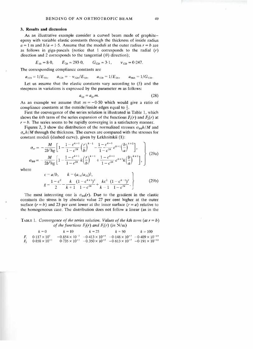
First the convergence of the series solution is illustrated in Table 1, which shows the kth term of the series expansion of the functions FJ(r) and F2 (r) at r = b. The series seems to be rapidly converging in a satisfactory manner.
Figures 2, 3 show the distribution of the normalized stresses oeeh/M and orrh/M through the thickness. The curves are compared with the stresses for constant moduJi (d shed curve), given by Lekhnitskii (1):
k 1 k 1 _ M [ l_c + (r)k-l l-C - k+l(b)k+l] }o - --- 1- - - c
C2krr 2b2hg 1 - C2k b 1 - a ' (29a)k k
__ ~ [ _ 1- C +1 (!.-)k-l 1- C -
1 k+l (~)k+l] °ee - 2b2hg 1 1 _ C2k k b + 1 _ C2k C k a '
where
(29b)
The most interesting one is 0ge(r). Due to the gradient in the elastic constants the stress is by absolute value 27 per cent higher at the outer surface (r = b) and 23 per cent lower at the inner surface (r = a) relative to the homogeneous c . e. The distribution does not follow a linear (as in the
TABLE 1. Convergence of the series solution. Values of the kth term (at r = b) of the functions F1(r) and fi(r) (in N/m)
k =0 k = 10k = 25 k = 50 k = 100 0·117 X 102 -0.854 X 10⁻² -0·413 X 10-4 -0'148 X 10-7 -00409 X 10- 14
0·858 X 10- 1 0·735 X 10- 1 -0.350 X 10⁻³ -0·813 X 10-7 -0'191 X 10- 13
FIG. 2. Distribution of the stress 06R at the cross-section in a curved beam of thickness h for the example case c nsidered. The broken line repre ents the case of a homogeneous beam with non-varying elastic con tants
throughout
1·2
1·0
0·8 ~ ~ 5 0·6
'"'" <l) .... v;
0-4
0·2
O·O-f--~-...,__-~-...,__-.....--...,__-~-...---~~
-0·0 0·2 0-4 0·6 0,8 1·0
r=(r-a)/h
FIG. 3. Stress distribution 0,.,. through the thickness in a curved beam of thjckness h for the example case considered. Th broken line represents the case of a homogeneous beam with Don-varying elastic constants throughout
51 BENDING OF AN ORTHOTROPIC BEAM
straight-bar case) or hyperb lic (as in the isotropic elementary strength-ofmaterials case) law. The other component of stress Orr is of much smaller magnitude and follows the same pattern; relative to the homogeneous case the curve is shifted s that the stress i increas d at points closer to the outside edge (r = b) and reduced t wards th inside edge (r = a). This component of stre s is neglect d in the elementary strength-of-m terials theory. Figure 4 shows the variation of the normalized hoop stress ueeh/M at the outside (solid line) and inside (dashed line) fibres as a function of the steepness parameter m in (28). The resulting curve is nonlinear with a higher slope at the larger values of m, which means that there is more stress reduction or increase per unit change in moduli at the large differential between elastic con tants on the inside and outside edges.
Table 2 shows the values for the Dormaliz d hoop stress uer/l/ M at the fibres on the outside and inside edge r = b and r = a, respectively. The range of the steepness parameter m in (28) is from 0 to -0·5, which in tum makes the ratio of the moduli at the inner and outer fibres between 1·0 and O· 5. The values of uer/l/M for the outer/inner fibres range from -10·56/ +13·84 for m = 0·0, that is constant moduli throughout, to -13.64/+11.25 for m = -0.5; that is, moduli on the inside edge being half that on the
outside. The maximum value of the radial stress arrh/M showed a small variation, ranging from 1·23 for m = 0·0 to 1·19 for m = -0·5.
A related case is the stress distribution in a ring with linearly varying elastic constants through the thickness under internal and/or external pressure. In this case Uo = 0 due to symmetry and C = 0 in (6). The solution follows the same pattern but now only two constants, A I and A 2 in expressions (19), need to be determined from the boundary conditions of internal (p) and external (q) pressures:
arrCa) = -p,
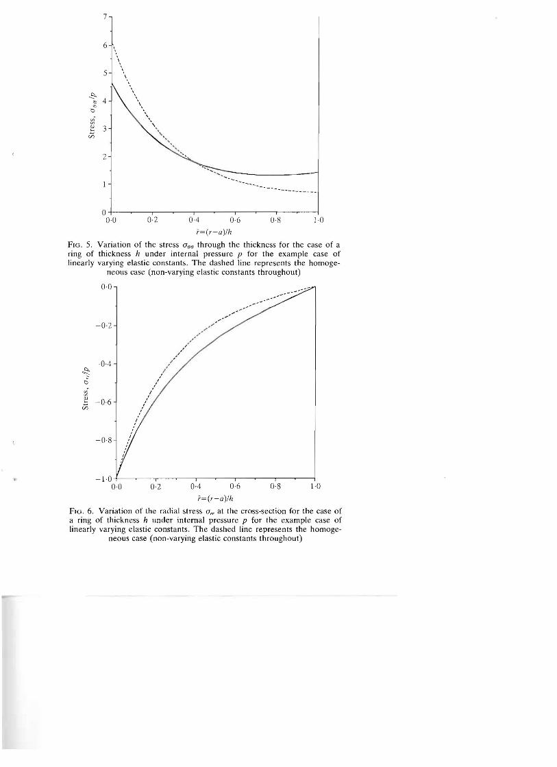
Results for the case of a ring loaded only on the inner contour (q = 0) and for material and radii data as in the previous curved-beam example are shown in Fig. 5 for the distribution of arr!p and in Fig. 6 for that of aoo/p. In these figures the re ults are compard with the homogeneous case (dashed line) which is given by Le hnitskii (2):
=~ [(!-)k-l _(~)k+l] =pCk+1k [(!-)k-l (~)k+l] a rr 1 -c2k b ' a oo 1 - 2k b + r ,r c
where c and k are given by (29b)I,2' It is seen that the radial (compre sive) stress arr is smaller in the case of variable moduli at all points through ut the thickness, whereas the hoop stress aoo at the outer edge (r = b) is twice that of the homogeneous case and about 25 per cent smaller at the inside edge (r = a). The effect of the steepness parameter m is illustrated in Table 3 which shows the values for the normalized hoop stress aoo/p at the fibres on the outside and inside edges of the ring r = band r = a, respectively. The values of aoo/p for the outer/inner fibres range from +0·70/+6·15 for m = 0·0, that is, constant moduli througbout, to + 1-41/ +4·65 for m = -0·5, that i , moduli on the inside edge being half that on the outside.
As for the displacements, for a ring under pressure, due to the rotational symmetry we have C = 0 and Uo = 0 and the displacement U r has radial dependence only. From (27)11 using the series solution (23) for the
7
6 ,, \,,
5 \ , , \
'"\" '. \
-'""'"
'''' ..2
-~~-
O+--~-,--~~--r-~-----r----r----r---.------j
0·0 0·2 0·4 0·6 0·8 1·0
r=(r-a)/h
FIG. S. Variation of the stress O(J(J through the thickness for the case of a ring of thickness h under internal pressure p for the example case of linearly varying elastic constants. The dashed line represents the homoge
neous case (non-varying elastic constants throughout)
0·0
-0·2
<:>. ~~
C 'J>" 'J>
~ Ul
-0·4
-0·6
-0·8
,/. /. .
,-~
,,/
,',/",
,/ /
,/ ,,/'
,,/ I,
, ,
/
-1·0 +--~-.--~----r-~---r--~--.----r---l
0·0 0·2 0·4 0·6 0·8 1·0
r=(r-a)/h
FIG. 6. Variation of the radial stress Orr at the cross-section for the case of a ring of thickness h under internal pressure p for the example case of linearly varying elastic constants. The dashed line represents the homoge
neous case (non-varying elastic constants throughout)
54 G. A. KARDOMATEAS
TABLE 3. Comparison of outside/inside fibre stresses in a ring under internal pressure p
FIG. 7. Distribution of the displacement u, for a ring of thickness h under internal pressure p for the example case of linearly varying lastic constants. The broken line represents the homogeneous case (non-varying
elastic constants throughout)
55 BENDING OF AN ORTHOTROPIC BEAM
stresses we obtain the displacement
Figure 7 shows the distribution of the radial displacement Ur through the thickness for the example case considered (solid line), as compared with the homogeneous, non-varying elastic-constant case (dashed line), given by
k 1 pC + [ (,)k (b)k]Ur = 1- eZk (alZ + a22k ) b - (alz - a2Zk ) -;: .
The displacement U r is seen to be higher for the non-bomogeneou case, especially near the inside edge.
REFERENCES 1. S. G. LEKHNITSKlI, Theory of Elasticity of an Anisotropic Elastic Body (Holden
Day, San Francisco 1963; Mir, Mosc w 1981). 2. --, Anisotropic Plates (Gordon & Breach, New York 1968). 3. J. IRVING and N. MULLINEUX, Mathematics in Physics and Engineering