Benefits of Coordinating Distribution Network Reconfiguration … · 2017-12-21 · systems (DESSs)...

Faculdade de Engenharia da Universidade do Porto

Benefits of Coordinating Distribution Network Reconfiguration with Distributed Generation and

Energy Storage Systems

Marco Rafael Meneses Cruz

Dissertação realizada no âmbito do Mestrado Integrado em Engenharia Electrotécnica e de Computadores

Major Energia

Orientador: Prof. Doutor João Paulo da Silva Catalão Co-orientador: Doutor Desta Zahlay Fitiwi

junho de 2016

ii

© Marco Rafael Meneses Cruz, 2016

iii

Resumo

O problema de integrar produção distribuída (DG) renovável em sistemas de distribuição

de energia está a tornar-se bastante crítico devido a razões técnicas, económicas e ambientais.

Atualmente, existe um consenso global de que a integração de recursos de origem renovável –

RESs, é altamente necessária para ter em conta o aumenta da procura de eletricidade e reduzir

a pegada de carbono global de produção de energia. Contudo, a integração em larga escala de

DG baseada em RES muitas vezes coloca desafios de ordem técnica no sistema, desde a

perspetiva da estabilidade, fiabilidade e qualidade de energia. Isto deve-se porque a integração

de RESs introduz uma expressiva variabilidade e incerteza no sistema de distribuição que faz

com que a operação, planeamento e controlo se tornem complexos. Consequentemente, um

esforço ao nível da integração é provável que seja suportado por certas tecnologias das redes

inteligentes smart grids e conceitos que tenham a capacidade de aumentar a flexibilidade de

todo o sistema de distribuição. Neste contexto, a integração de sistemas distribuídos de

armazenamento de energia (DESSs) em conjunto com DGs, juntamente com a capacidade de

comutação da rede e/ou reforço da rede, pode aumentar significativamente a flexibilidade do

sistema, e por isso, beneficia a produção RES.

Este trabalho apresenta um novo método para quantificar os impactos associados a DESS

assim como a comutação da rede e/ou reforço ao nível de integração de produção renovável

no sistema. Para executar esta análise, dois modelos foram desenvolvidos, um modelo de

programação linear inteira mista (MILP) e um modelo baseado em Algoritmos Genéticos (GA).

Estes modelos têm em consideração o reforço na rede de distribuição e/ou comutação em

coordenação com a integração de tecnologias DGs baseadas em RES e DESS.

As metodologias propostas são testadas nos sistemas de 16 e 33-nós do IEEE. Os resultados

da análise mostram a capacidade de comutação/reforço da rede e a integração de DESS em

suportar significativamente a integração em larga escala de DGs renováveis.

Palavras-Chave Algoritmo Genético (acrónimo em inglês, GA), Comutação da Rede, Produção Distribuída

(acrónimo em inglês, DG), Programação Linear Inteira Mista (acrónimo em inglês, MILP),

Reforço da Rede, Sistemas Renováveis de Energia (acrónimo em inglês, RESs), Sistemas

Distribuídos de Armazenamento de Energia (acrónimo em inglês, DESS).

iv

v

Abstract

The issue of integrating renewable distributed generation (DG) in power distribution

systems is becoming critical because of technical, economic and environmental reasons.

Nowadays, there is a global consensus that integrating renewable energy sources—RESs, is

highly needed to meet an increasing demand for electricity and reduce the overall carbon

footprint of energy production. However, large-scale integration of RES-based DGs often poses

a number of technical challenges in the system, from stability, reliability and power quality

perspectives. This is because integrating RESs introduces significant operational variability and

uncertainty to the distribution system, making operation, planning and control rather

complicated. Hence, such a high level integration effort is likely to be supported by certain

smart-grid technologies and concepts that have the capability to enhance the flexibility of the

entire distribution system. Framed in this context, the integration of distributed energy storage

systems (DESSs) jointly with DGs, along with the network’s switching capability and/or network

reinforcement, significantly improves the flexibility of the system, thereby increasing chances

of accommodating large-scale RES power.

This work presents a novel method to quantify the impacts of installing DESS as well as

network switching and/or reinforcement on the level of renewable power integrated in the

system. To carry out this analysis, two models are developed, mixed integer linear programming

(MILP) and Genetic Algorithm (GA) based models. These models take into account the

distribution network reinforcement and/or switching in coordination with integrating RES-based

DGs and DESS technologies.

The proposed methodologies are tested on 16- and 33-node systems. The results show the

capability of network reinforcement/switching and DESS integration in significantly supporting

large-scale integration of renewable DGs.

Keywords

Genetic Algorithms (GA), Network Switching, Distributed energy storage systems, Distributed

Generation, Mixed Integer Linear Programming (MILP), Network Reinforcement, Renewable

Energy Sources (RESs), Energy Storage Systems (ESS).

vi

vii

Acknowledgements

The years that I spent in the Faculty of Engineering of the University of Porto are thanks to

my parents, who were the moral and financial support for this personal project. The knowledge

that I’ve got is due to an extraordinary group of professors in FEUP, that made me a potential

candidate to be an engineer. To all classmates with whom I had the pleasure of depriving is

also a major aspect because without group work, and friends, life is more complicated. Hence,

many thanks to my friends who were always there with me in good times and bad times. To my

supervisor, Professor João Catalão, many thanks for bringing me this challenge, and to Desta

and Sergio, many thanks for always being available to help. A thank you to all who have made

this experience also a lesson, enabling my goals in the Master in Electrical and Computer

Engineering to be reached.

Virtus Unita Fortius Agit

viii

x

Table of Contents

Chapter 1 ........................................................................................................ 1

Introduction................................................................................................ 1

1.1 – Background ...................................................................................... 1

1.2 – Problem Statement ............................................................................. 2

1.3 – Objectives ........................................................................................ 5

1.4 - Methodology ..................................................................................... 5

1.5 – Thesis Structure ................................................................................. 6

Chapter 2 ........................................................................................................ 5

Literature Review ......................................................................................... 5

2.1 – Chapter Overview............................................................................... 5

2.2 – Distribution System Reconfiguration ........................................................ 5

2.3 – Distributed Generation and Distribution System Reconfiguration ..................... 7

2.4 - Energy storage system and Distributed Generation .................................... 11

2.5 – Distributed System Reconfiguration, Distributed Generation and Energy Storage

Systems ......................................................................................... 15

2.6 – Summary ....................................................................................... 16

Chapter 3 ...................................................................................................... 19

Problem Formulation - A Mixed Integer Linear Programming Approach ...................... 19

3.1 – Algebraic Formulation of the Joint Planning Problem ................................. 19

3.2 – Summary ....................................................................................... 26

Chapter 4 ...................................................................................................... 29

Problem Formulation and Solution -Genetic Algorithms Approach ............................ 29

4.1 – An overview of Genetic Algorithms ........................................................ 29

4.2 – Genetic Algorithms: Formulation .......................................................... 35

4.3 – Summary ....................................................................................... 38

xi

Chapter 5 ...................................................................................................... 39

Case Studies, Results and Discussion ................................................................ 39

5.1 – Mixed Integer Linear Programming based Optimization .............................. 39

5.2 – Genetic Algorithm Results .................................................................. 43

5.3 – Summary ........................................................................................ 56

Chapter 6 ...................................................................................................... 59

Conclusions and Future Works ........................................................................ 59

6.1 – Conclusions .................................................................................... 59

6.2 – Future Works .................................................................................. 60

6.3 – Works Resulting from this Thesis ........................................................... 60

References ............................................................................................... 62

xi

List of Figures

Figure 2.1 - The main advantages of integrating Distributed Generators in the distribution system (adapted from [24]). .......................................................................... 9

Figure 2.2 - The main reasons to adopt Energy Storage Systems in network (adapted from [52]) ..................................................................................................... 12

Figure 2.3 - Integration of various technologies in the distribution system- illustrative figure (Figure adapted from [65] and [66]. ....................................................... 15

Figure 4.1 - Possible chromosome representation ..................................................... 30

Figure 4.2 - Flow Chart of the proposed GA. ........................................................... 37

Figure 5.1 - 33-bus radial distribution system. ......................................................... 40

Figure 5.2 - Optimal DG location in Cases 3, 4, 5 and 6 .............................................. 41

Figure 5.3 - Average voltage profiles in the system under different cases. ....................... 42

Figure 5.4 - Optimal locations of DGs and ESSs under Case 6 (Opened switches 28-29, 8-21, 9-1 ................................................................................................... 42

Figure 5.5 - Total system losses profile. ................................................................. 43

Figure 5.6 - 16-bus radial distribution system [67]. ................................................... 44

Figure 5.7 - New topology of the distribution system from Case 2. ................................ 46

Figure 5.8 - Voltage comparison between base case and reconfiguration......................... 46

Figure 5.9 - Reconfiguration under different feeders cost. .......................................... 47

Figure 5.10 - Voltage profile of Case 4-F2. .............................................................. 47

Figure 5.11 - Voltage comparison between Case 7 and Base Case .................................. 48

Figure 5.12 - Optimal location for DG and reconfiguration in Case 7. ............................. 49

Figure 5.13 - Size and placement of DGs in the 16-bus distribution system. ..................... 49

Figure 5.14 - Convergence process in Case 2. .......................................................... 50

xii

Figure 5.15 - Convergence process in Case 7. .......................................................... 50

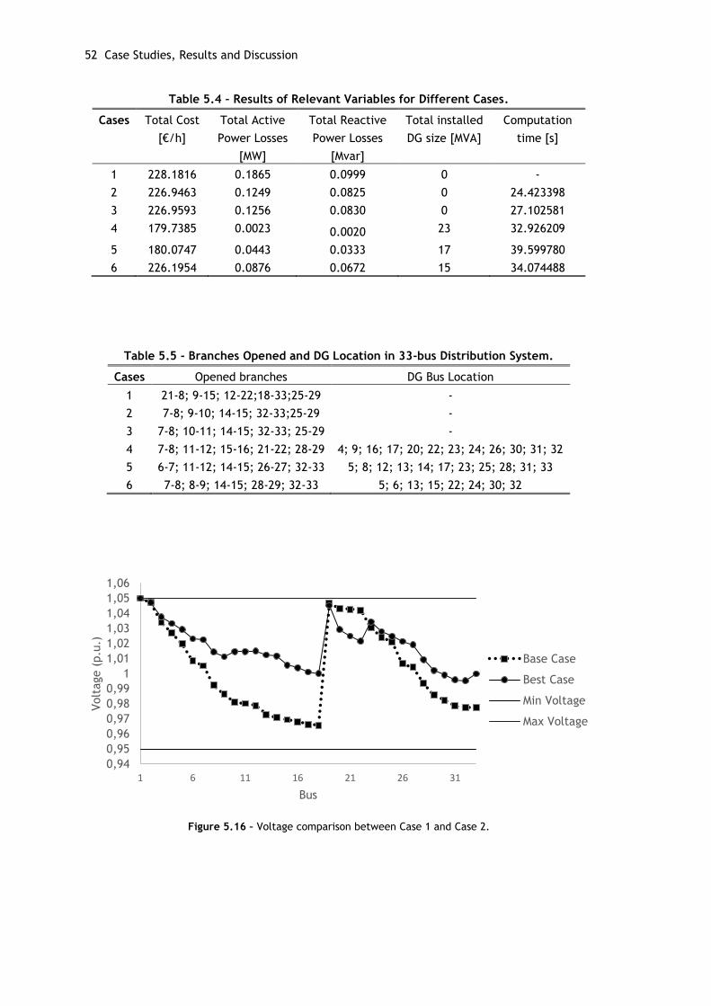
Figure 5.16 - Voltage comparison between Case 1 and Case 2. ..................................... 52

Figure 5.17 - Voltage comparison between base Case 1, Case 2 and Case 3. ..................... 53

Figure 5.18 - Voltage comparison between Case 1 and Case 4, 5, 6. .............................. 53

Figure 5.19 – Convergence process in Case 4 and 5 ................................................... 53

Figure 5.20 – Convergence process in Case 6 ........................................................... 54

Figure 5.21 - Configuration in Case 2. ................................................................... 55

Figure 5.22 - DG size and placement in Cases 4, 5 and 6. ........................................... 55

Figure 5.23 - Configuration and DG placement Case 4. ............................................... 56

xiii

List of Tables

Table 5.1 - Results of Relevant Variables for Different Cases. ...................................... 41

Table 5.2 - Results of Relevant Variables for Different Cases ....................................... 45

Table 5.3 - Opened Branches and Location of DG. .................................................... 46

Table 5.4 - Results of Relevant Variables for Different Cases ....................................... 52

Table 5.5 - Branches Opened and DG Location in 33-bus Distribution System. ................... 52

xiv

Acronyms and Nomenclature

Acronyms

AC Alternating Current

AHP Analytic Hierarchic Process

ACA Ant Colony Algorithm

ABC Artificial Bee Colony

AIS Artificial Immune System

ARMA Auto Regression Moving average

DESS Distributed Energy Storage System

DQPSO Decimal coded Quantum Particle Swarm Optimization

DOE Department of Energy

DC Direct Current

DG Distributed Generation

DSR Distribution Systems Reconfiguration

EWD Edge Window Decoder

EDS Electrical Distribution Systems

EWS Energy Management Strategy

ENS Energy Not Supplied

ESS Energy Storage System

EU European Union

EA Evolutionary Algorithm

EPSO Evolutionary Particle Swarm Optimization

FNSGA Fast Nondominated Sorting Guided Genetic Algorithm

GA Genetic Algorithm

HSA Harmony Search Algorithm

HOMER Hybrid Optimization Model for Electric Renewables

IEA International Energy Agency

MILP Mixed Integer Linear Program

MINLP Mixed Integer Non Linear Programming

MISOCP Mixed-Integer Second-Order Cone Programming

MPSO Modified Particle Swarm Optimization

xviii

MACS Multiagent Control System

MMP Multi-objective Mathematical Programming

NPV Net Present Value

NLMIP Non-Linear Mixed Integer Programming

OPF Optimal Power Flow

PSO Particle Swarm Optimization

RHC Receding Horizon Control

RES Renewable Energy Sources

SA Scenario Analysis

TS Tabu Search

NSGA-II Non-dominated Sorting Genetic Algorithm II

TSC Total Supply Capability

UVDA Uniform Voltage Distribution based constructive Reconfiguration Algorithm

UPS Uninterruptible Power Supply

US United States

Vaccine-AIS Vaccine-enhanced Artificial Immune System

Nomenclature

A. Sets/Indices

𝑖/Ω𝑖 Index/set of buses

𝑔/𝛺𝑔/ 𝛺𝐷𝐺 Index/set of generators/DGs

𝑘/𝛺𝑘 Index/set of branches

𝑠/𝛺𝑠 Index/set of scenarios

𝑡/𝛺𝑡 Index/set of planning stages

𝑤/𝛺𝑤 Index/set of snapshots

𝜍/𝛺𝜍 Index/set of substations

B. Parameters

𝐸𝑅𝑔𝑁 , 𝐸𝑅𝑔

𝐸 , 𝐸𝑅𝜍𝑆𝑆 Emission rates of new and existing DGs, and energy purchased, respectively

(tCO2e/MWh)

𝐼𝐶𝑔,𝑖, 𝐼𝐶𝑘 , 𝐼𝐶𝑒𝑠,𝑖 Investment cost of DG, line and energy storage, respectively (M€)

𝐿𝑇𝑔, 𝐿𝑇𝑘 , 𝐿𝑇𝑡𝑟 , 𝐿𝑇𝑒𝑠 Lifetimes of DG, distribution line, transformer and energy storage system,

respectively (years)

𝑀𝐶𝑒𝑠, 𝑀𝐶𝑡𝑟 Maintenance cost of storage per year (M€)

𝑀𝐶𝑔𝑁, 𝑀𝐶𝑔

𝐸 Maintenance costs of new and existing DGs (M€/yr)

𝑀𝐶𝑘𝑁, 𝑀𝐶𝑘

𝐸 Maintenance cost of new and existing line (M€/yr)

𝑂𝐶𝑔,𝑖,𝑠,𝑤,𝑡𝑁 , 𝑂𝐶𝑔,𝑖,𝑠,𝑤,𝑡

𝐸 Operation cost of unit energy production by new and existing DGs (€/MWh)

𝜆𝑠,𝑤,𝑡𝐶𝑂2𝑒 Price of emissions (€/tons of CO2 equivalent)

𝜆𝑠,𝑤,𝑡𝜍

Price of electricity purchased (€/MWh)

𝜌𝑠, 𝜋𝑤 Probability of scenario s and weight (in hours) of snapshot group w

𝜐𝑠,𝑤,𝑡 Penalty for unserved power (€/MW)

𝜂𝑐ℎ,𝑒𝑠 Charging efficiency

xix

𝜇𝑒𝑠 Scaling factor

C. Variables

𝛿𝑖,𝑠,𝑤,𝑡 Unserved power at node i

𝐷𝑠,𝑤,𝑡𝑖 Active power demand at node i

𝑃𝑔,𝑖,𝑠,𝑤,𝑡𝑁 , 𝑃𝑔,𝑖,𝑠,𝑤,𝑡

𝐸 Active power produced by new and existing DGs

𝑃𝜍,𝑠,𝑤,𝑡𝑆𝑆 Active power imported from grid

𝑢𝑔,𝑖,𝑡, 𝑢𝑘,𝑡 Utilization variables of existing DG and lines

𝑥𝑔,𝑖,𝑡 , 𝑥𝑒𝑠,𝑖,𝑡 , 𝑥𝑘,𝑡 Investment variables for DG, storage systems and distribution lines,

respectively

𝜑𝑘,𝑠,𝑤,𝑡 Losses associated to each feeder

𝐸𝑒𝑠,𝑖,𝑠,𝑤,𝑡 Reservoir level of ESS

𝐼𝑒𝑠,𝑖,𝑠,𝑤,𝑡𝑑𝑐ℎ , 𝐼𝑒𝑠,𝑖,𝑠,𝑤,𝑡

𝑐ℎ Discharging/charging indicator variables

𝑃𝑒𝑠,𝑖,𝑠,𝑤,𝑡𝑑𝑐ℎ , 𝑃𝑒𝑠,𝑖,𝑠,𝑤,𝑡

𝑐ℎ Discharged/charged power

𝑥𝑡𝑟,𝑠𝑠,𝑡 Transformer investment variable

D. Functions

𝐸𝐶𝑡𝑆𝑆 Expected cost of energy purchased from upstream

𝐸𝑁𝑆𝐶𝑡 Expected cost of unserved power

𝐸𝑚𝑖𝐶𝑡𝐷𝐺 Expected emission cost of DG power production

𝐸𝑚𝑖𝐶𝑡𝑁 , 𝐸𝑚𝑖𝐶𝑡

𝐸 Expected emission cost of power production using new and existing DGs,

respectively

𝐸𝑚𝑖𝐶𝑡𝑆𝑆 Expected emission cost of purchased power

𝐼𝑛𝑣𝐶𝑡𝐷𝑁𝑆, 𝑀𝑛𝑡𝐶𝑡

𝐷𝑁𝑆 NPV investment/maintenance cost of DNS components

𝐼𝑛𝑣𝐶𝑡𝐷𝐺 , 𝑀𝑛𝑡𝐶𝑡

𝐷𝐺 , 𝐸𝐶𝑡𝐷𝐺 NPV investment/maintenance/expected energy cost of DGs, respectively

𝐼𝑛𝑣𝐶𝑡𝐿𝑁 , 𝑀𝑛𝑡𝐶𝑡

𝐿𝑁 NPV investment/maintenance cost of a line

𝐼𝑛𝑣𝐶𝑡𝐸𝑆, 𝑀𝑛𝑡𝐶𝑡

𝐸𝑆 NPV investment/maintenance cost of ESS

xx

Chapter 1

Introduction

1.1 – Background

Driven by technical, economic, environmental and structural factors, the integration of

Renewable Energy Sources (RESs) in power systems has been increasing steadily. Furthermore,

global concerns such as climate change, energy dependence and security and other related

issues are forcing policy makers and states to introduce new energy policies (RES policies, in

particular) that support the development and utilization of RESs. The favorable agreement of

states to curb emissions and mitigate climate change is also expected to further accelerate RES

integration in power systems (particularly, at a distribution level). The level of Distributed

Generation (DG) deployed in distribution network systems follows an upward trend, and there

is a general consensus that DGs will immensely contribute to the efforts of addressing a

multitude of the aforementioned global and local concerns including collective (and/or

individual) RES integration targets set forth by different entities.

The availability of several matured DG technologies and their decreasing cost trends, along

with constraints in the construction of new transmission lines, increased customers’ demand

for highly reliable electricity etc. has been encouraging considerable investments in DGs

(particularly, renewable types such as wind and solar power). However, large-scale integration

of DGs in distribution network systems may sometimes bring technical problems to the system

such as voltage rise issues. Such challenges need to be resolved if the system is to support the

integration and full (efficient) utilization of massive DG power. One way is to properly allocate

DGs in the system. The purpose of DG placement (allocation) is to find the optimal location and

size of DGs (generally non-conventional energy sources) in the system, close to the end

consumers.

In particular, large-scale integration of RES-based DGs often poses a number of technical

challenges in the system from the stability, reliability and power quality perspective. This is

because integrating RESs introduces significant operational variability and uncertainty to the

distribution system, making operation, planning and control rather complicated.

2 Introduction

Hence, such a high level integration effort is likely to be supported by certain smart-grid

technologies and concepts that have the capability to enhance the flexibility of the entire

distribution systems. Energy Storage Systems (ESSs) can play a vital role integrating variable

energy sources. In addition, Reconfiguration of Distribution System (RDS) can be very important

because RDS can considerably enhance the flexibility of the system and voltage profiles,

thereby increasing chances of accommodating large-scale RES power.

1.2 – Problem Statement

RESs make a crucial part of the solution for environmental sustainability; hence, they will

play an important role in power systems. The integration of RESs should, in principle, reduce

the risk of fuel price volatility and geopolitical pressures and ensure that these do not pose a

significant impact on the overall public welfare. However, large-scale penetration of RESs will

necessarily involve a process of adapting and changing the existing infrastructure because of

their intrinsic characteristics, such as intermittency and variability. The growing need for

intermittent RESs, in conjunction with the electrical mix changes in the long-term, will

probably affect the distribution and transmission systems. In this context, a change in power

generation options, resulting from a high contribution of RESs, may require network grid

updates. Regulatory agencies are heavily committed to increase RES integration, not only due

to environmental but also technical and economic reasons. The main challenge with most of

RESs is their inherent variability and uncertainty, making operation, control and planning very

complicated. DG penetration increases the variation of voltage and current in the network.

Hence, increasing DG penetration may have a negative or a positive impact depending on

various factors such as the size of the system and the loads type, requiring modeling and

simulations to assess its impact. If not properly planned, this may lead to an uncertain increase

in the feeders’ power flows, resulting in network congestion and increased losses in the

network. However, the integration of ESS along with RESs has become one of the most viable

solutions to facilitate the increased penetration of DG resources. Energy storage systems level

the mismatch between renewable power generation and demand. This is because these devices

store energy during periods of low electricity demand (price) or high RES power production,

and then release it during periods of peak demand and low RES production. Therefore, in

addition to their technical support to the system, ESSs bring substantial benefits for end-users

and DG owners through reliability and power quality improvement as well as cost reduction.

Besides, ESSs are being developed and applied in power grids to cope with a number of issues

such as smoothing the energy output from RESs, improving the stability of the electrical system,

etc. ESSs also increase savings during peak hours and minimize the impact of intermittent

generation sources, leading to a more efficient management of the integrated system. Despite

the high capital costs of many ESS technologies, their deployment in distribution systems is in

the upward trend. Cost-cutting and the strong need of integrating RES-based DGs is expected

to push the demand for the simultaneous deployment of ESSs in distribution network systems.

In other words, distributed ESSs will increase dramatically in the years to come. Hence, proper

planning of such systems is crucial for a healthy operation of the system as a whole. This relates

to developing appropriate mathematical models and algorithms that lead to the optimal

placement, timing and sizing of DGs and ESSs in the system, which is one of the problems

addressed in this thesis.

Objectives 3

Electrical distribution systems are interconnected by switches but predominantly operated

radially. These switches are often used for emergency purposes such as to evade load

curtailment during fault cases. However, the system can be reconfigured to find the best

topology that minimizes power losses in the system and improve operational performance. This

in turn improves the flexibility in the system, which may help the system to accommodate

(absorb) more variable power. Investigating the capability of network switching and/or

expansion along with ESS deployment in RES integration level is another problem addressed in

this thesis.

1.3 – Objectives

This thesis aims to achieve the following goals:

To carry out a comprehensive state-of-the-art literature review on the subject areas

of distribution network reconfiguration, DG and ESS integrations, which forms a basis

for defining the problem addressed in this thesis;

To develop mathematical models for jointly optimizing distribution network

reconfiguration, optimal placement, timing and sizing of ESS and RES-based DGs

considering uncertainty and variability inherent to such problems;

To carry out case studies and perform relevant analysis of results;

To analyse the effects of distribution reconfiguration in the distribution networks;

To carry out quantitative and qualitative analysis in relation to the influences optimal

sizing, location and timing of DGs and ESSs along with distribution network

reconfiguration on relevant system variables in the distribution network.

1.4 - Methodology

The work in this thesis involves both qualitative and quantitative analysis regarding the

impact of joint integration ESSs, network switching (reconfiguration) and reinforcement on the

level of DG integration (particularly, focusing on RESs). In order to achieve the objectives, set

in this thesis, a set of different mathematical simulation models are developed.

In order to solve the proposed objectives were created two optimization models. The first

proposed optimization model is coded by multi-objective Stochastic Mixed Integer Linear

Program (S-MILP) to a planning horizon of three years and solved with GAMS, considering the

operational variability and uncertainty of variable power resources along with reconfiguration

and energy storage systems.

4 Introduction

Also, a second optimization model proposed is coded by a GA and solved using the MatPower

(package of MATLAB) optimal power flow (OPF). GA considers: 1) one snapshot of the

distribution system to solve reconfiguration and 2) one snapshot of the distribution system to

solve reconfiguration with optimal size and location of DGs. To reach at best reconfiguration

of the distribution network GA will raffle the connected branches (1 or 0), proceed to resolution

of OPF with the configuration given and keep the OPF costs DG’s placement and size is done at

the same time by raffling the nodes were DGs are connected by the two-third theory. Size of

DGs is done by takin an interval between 1 and 4 MW and raffle an integer number between

that interval. A comparison between the base case and the best case given by GA is done,

comparing reconfiguration only and reconfiguration with placement and size of DGs.

The objective for the two methods is minimization of costs. In the case of S-MILP the total

costs of the system (objective function) is composed of Net Present Value (NPV) of five cost

terms: 1) investment costs, 2) costs of maintenance, 3) cost of energy in the system, 4) cost of

unserved power and 5) total emission costs. For GA model the costs are given by the optimal

power flow, consequently the cost of energy provided to the demand is minimized.

1.5 – Thesis Structure

The thesis is organized as follows. Chapter 2 presents a literature review of relevant works

on the subject area of the thesis. A theoretical overview of the genetic algorithm, along with

the descriptions of the entire solution process, is presented in Chapter 3. The stochastic

mathematical models developed in this thesis are described in Chapter 4. Case studies, results

and discussions are presented in Chapter 5. Chapter 6 gathers the relevant conclusions drawn

from the numerical results, and shows directions for future work.

Chapter 2

Literature Review

2.1 – Chapter Overview

This chapter presents an extensive review of related works on subject area of distribution

systems planning particularly focusing on the problems of distribution network reconfiguration,

distribution generation and energy storage allocation and sizing in distribution network

systems. The reviewed works are largely structured based on the methodologies used to solve

the aforementioned problems.

2.2 – Distribution System Reconfiguration

2.2.1 – Motivation of DSR

Electrical distribution systems link high voltage transmission systems and the end-

consumers. They are often designed in a slightly meshed manner but normally operated in a

radial configuration because of a number of reasons such as reduction of costs, uncomplicated

coordination of protection systems, reduced occurrence of faults, better control power flows

and voltage profile. Because of such reasons, maintaining the radial topology of the network

systems is very critical. The reasons further explain the need for optimizations of distribution

network systems to obtain the optimal radial topology [1].

For the system to operate on a permanent basis, it is desirable to increase its efficiency

and reduce its operating costs. One way to achieve this is by minimizing losses [2]. Some

techniques used to reduce system losses are increasing the voltage level, cable replacement,

installation of condensers and/or distribution systems reconfiguration (DSR). Among these

techniques, the reconfiguration is the most attractive for the electricity distribution company

because it allows the use of resources that already exist in the system. Consequently, DSR can

be implemented by changing the status of the switches that connect/disconnect the branches

of the system, in order to obtain a radial topology [3]–[20]. Reconfiguration can be done for

numerous reasons, as in normal or emergency operation conditions.

6 Literature Review

In [21] authors show that losses in distribution network systems constitute more than 75%

of the total system losses, contributing to a 40% of the total cost incurred to deliver power and

80% of customer reliability. The losses are also classified as technical and non-technical losses.

Non-technical losses include unauthorized line tapping, meter ampering, inaccurate meter

reading, subsidies, unmetered public lighting etc. They can be reduced by monitoring, creating

awareness, installing accurate metering devices etc. Technical losses occur due to flow of

electric current. They cause economic damage.

The DSR problems can be formulated as single-objective or multi-objective optimizations.

In such optimization problems, there are two objectives that stand out, minimization of losses,

especially in mono-objective approaches, and in multi-objective approaches besides the

previous target, also operating costs minimization and maximization of the profit. It should be

noted that in the multi-objective approach, the objective functions can be conflicting, in which

case, the optimum solution is the result of a trade-off between multiple objectives [2].

Due to its explicit benefits (mentioned earlier), there has been a growing number of

literature on the DSR problem over the past years, and it still remains an actual working topic.

Generally, the goal of network reconfiguration is not only to reduce power losses but also to

improve voltage profile, network reliability and economic operations. Therefore, DSR aims to

find the best topology of the system taking into account power losses, energy demand,

operational performance and other relevant determining factors.

Based on the solution techniques applied to solve DSR problems, the literature on DSR can

be broadly classified into two categories: 1) mathematical techniques; 2) heuristic and

metaheuristic techniques [22].

2.2.2 – Mathematical Solution Techniques in DSR

In the literature, a number of exact techniques have been widely employed to solve DSR

problems, such mixed-integer linear programming (MILP) [3], [8] mixed-integer second-order

cone programming (MISOCP) [4], analytic hierarchic process (AHP) [9]. Paterakis et al. in [3]

propose a MILP DSR optimization model, which is formulated as a multi-objective mathematical

programming (MMP) problem. The objective function constitutes the minimization of the active

power losses and the minimization of commonly used reliability indices, which are explicitly

treated within the MILP formulation. In [4], Chen et al. presents the assessment of distribution

network total supply capability (TSC) value modelled as a MISOCP optimization problem. Gupta

et al. [8] suggest a new MILP model which combines power and reliability objectives into a

single objective function. A real time configuration based on load rate analysis is proposed by

Pfitscher et al. [9]. AHP is applied in a multicriteria decision making and analyzing of

parallelism of feeders using Euler’s discretization method to make sure that the reconfiguration

outcome does not violate radiality constraints.

The mathematical techniques have been less commonly used mainly due to computational

limitations. However, this paradigm has been changing with increased processing capability of

computing machines in addition to the new processing styles that have been developed recently

such as cloud computing. Heuristics and metaheuristics techniques have been employed in

recent years. Several of these techniques are combined in order to exploit the best

characteristic of each technique.

Heuristic and Metaheuristic Solution Techniques in DSR 7

2.2.3 - Heuristic and Metaheuristic Solution Techniques in DSR

The mathematical computational complexity of the DSR problem (mainly due to its

combinatorial, non-convex and nonlinear nature) has led to the extensive use of heuristic and

metaheuristic techniques in the literature by researchers. Some of these methods which have

been widely used to solve the aforementioned problem include genetic algorithm (GA) [5], [7],

[10], [11], [16], [18], [19], particle swarm optimization (PSO) [14] and others. A new non

dominated sorting guided GA (FNSGA) has been used to solve a multi-objective problem by

Eldurssi and O’Connell [5]. For automated reconfiguration, an enhanced GA has been suggested

by Duan et al. [7], with the aim of determining the optimal network configuration that leads

to the minimum power losses and/or the maximum system reliability. Torres et al. [10] uses a

GA for solving a DSR problem with purpose of minimizing real power losses while satisfying

several system operating constraints. A codification strategy based on the edge window decoder

(EWD) encoding technique that only leads to radial configurations has been employed. Even if

the DSR problem has been formulated as a MILP optimization in [8], authors use GA to obtain

the best compromising radial operating configuration. Cebrian and Kagan [16] address the

reconfiguration of distribution networks considering power quality indices by formulating such

a problem as non-linear mixed integer programming optimization, which is then solved by an

evolutionary algorithm (EA).

In [11], the DSR optimization is formulated as a single objective problem, encompassing

only the active power losses minimization. To find the optimal or near-optimal configuration

each candidate configuration is analyzed in two steps. First, the candidate topology is assessed

whether or not it is a valid radial configuration. Second, if the first condition is fulfilled, a

power flow module is run from which steady state variables are determined. Meshed heuristic

algorithm has been developed by Mena and García [13] to solve the reconfiguration problem

with an objective function of network losses minimization. Niknam and Farsani [14] have

combined a hybrid EA with a self-adaptive discrete PSO to determine the statuses of

sectionalizing switch numbers, and a self-adaptive binary PSO to determine the statuses of tie

switches. This way, the distribution network is optimally reconfigured maintaining its radial

topology. Abul’Wafa [15] propose a heuristic approach, embedded in a load flow algorithm that

gives precise branch currents, node voltages and system power losses. Sahoo and Prasad [17]

consider voltage stability as the objective function, and the resulting DSR problem is solved

using a fuzzy GA. Mendoza et al [18] minimize losses via reconfiguration, which is solved using

a generic GA. The GA technique is based on the creation of an initial population of feasible

individuals. A fuzzy mutated GA is proposed by Prasad et al. [19] for reconfiguration of

distribution systems with a new chromosome representation of the network and a fuzzy

mutation control.

2.3 – Distributed Generation and Distribution System Reconfiguration

2.3.1 – Overview of Distributed Generation

As mentioned in the previous section, DSR can be characterized as changing the statuses of

various switches that connect/disconnect the branches of the system in order to obtain a radial

topology which improves overall system performance and efficiency.

8 Literature Review

The subsequent topology, yet, depends on many input parameters and needs to be updated

on a daily, monthly, or periodic basis to adjust to the changes in the system operating condition.

With increased penetration of variable renewable Distributed Generation (DG), one is more

likely to experience constantly changing system conditions. As a result, the need for network

reconfiguration increases because this enhances the flexibility of the system, which is useful to

cope with operational variations.

The purpose of distributed generation (DG) placement is to connect distributed generating

units, generally based on non-conventional energy sources, at end consumers. According to the

International Energy Agency (IEA), there are five key factors that have significantly increased

interest in distributed generations [23]: 1) development in DG technologies, 2) constraints on

construction of new transmission lines, 3) increased customer demand for highly reliable

electricity, 4) electricity market liberalization and 5) concerns about climate change.

Distributed generation (DG) implies the deployment of small generation units (from 1kW to

1MW) connected to distribution network and close to the end-consumers [24]. In addition, unlike

conventional electrical networks that have unidirectional power flow, the introduction of DG

leads to a bidirectional power flow.

Technical, economic and environmental advantages, as well as the disadvantages of DG

integrations are presented [23],[24].

DG is classified in renewable energy sources (RES) and non-renewable energy sources. RES-

based DGs are classified as photovoltaic (PV), wind, hydro, geo-thermal, tidal and bio fuel. The

non RES-based DG includes the diesel generator[23]. Some of the advantages of integrating

DG’s [21], [25] are summarized in Figure 2.1. Distribution networks have been designed to handle

unidirectional power flow. The introduction of DGs can have positive or negative impact on

the distribution network systems [23], [24]. The main negative impacts include:

Integration of DGs can result in overvoltage issues. This is not a problem when DG

is connected to a system with low voltage issues. However, for weakly loaded

systems, DG integration may result in high voltage problems interfering with

standard voltage regulation practices. RES based DGs can especially worsen the

voltage profile due to their intermittent nature.

The impact on protection co-ordination given that the power grids are designed to

operate for unidirectional power flow.

The impact on harmonics as a result of integrating RES based DGs, which often

require power electronic interfaces, major sources of harmonics injected in the

system.

The impact on reactive power management can be an issue with DG units which are

incapable of providing reactive power. Hence, if DG units are not properly located

and sized, they can have negative effects on the system. When connected to the

network, various DG technologies can lead to high levels of reliability and security

issues [24], [23], [26].

DG Allocation in Distribution Systems—A Literature Review 9

Despite the steady growth of DG systems in recent years, there are still certain barriers

(technical, economic, regulatory) that restrict progress toward a new paradigm of electric

networks [24].

2.3.2 – DG Allocation in Distribution Systems—A Literature Review

Georgilakis and Hatziargyriou [27] present a review on the models, the methods and future

research of optimal DG placement in electrical distribution systems. Typically, the DG

allocation is a complex optimization problem that deals with the optimal planning of DGs in

existing distribution networks while respecting a number of technical, economic and

environmental constraints. Such an optimization work should lead to the optimal location and

size as well as the installation timing of DGs. The DG planning optimization problem is usually

difficult to solve using traditional mathematical methods because it is a nonlinear, non-convex

and combinatorial problem.

A number of approaches and methods have been proposed in the literature for

simultaneously restructuring of distribution network, and placement and sizing of DGs. Majority

of the previous works in this regard aim to reduce active power losses and improve the voltage

profile [28], [29]. The solution methods applied for solving the problems can be broadly

classified as 1) mathematical, 2) heuristic and meta-heuristic 3) hybrid types [21].

Mathematical techniques including MILP [30], [31], MISOCP [32] and multi-period optimal

power flow (MP-OPF) [33] have been employed in the literature to resolve the DG planning

problem. Haghighat and Zeng [30] propose a method to find a robust radial network topology

with minimum losses of a distribution system considering uncertainty in load and renewable

generation. The resulting problem is formulated in a MILP two-stage optimization framework.

Figure 1 - The main advantages of integrating Distributed Generators in the distribution system.

Figure 2.1 - The main advantages of integrating Distributed Generators in the distribution system (adapted from [24]).

10 Literature Review

The DSR problem aims to minimize losses under uncertain load and generation. The problem

has been decomposed in a master-slave structure. Ghamsari et al. [32] have developed a

MISOCP mathematical model to analyze the possibility and economics of an hourly

reconfiguration in the presence of renewable energy resources. The objective function of the

resulting problem is to minimize daily network losses via applying hourly reconfigurations,

formulated as a MISOCP problem which is then solved using the MOSEK solver. Capitanescu et

al. [33] proposes a multi-period OPF approach for assessing the improvement of DG hosting

capacity of distribution systems by applying static or dynamic reconfiguration, together with

active network management schemes. Muñoz-Delgado et al. [31] report a MILP optimization

model whose objective is to minimize the net present value of the total cost including the costs

related to investment, maintenance, production, losses, and unserved energy. The costs of

energy losses are modeled by a piecewise linear approximation. Tahboub et al. [6] use MINLP

to formulate the DSR and a fuzzy C-means clustering algorithm is used to obtain representative

centroids from annual DG and power demand profiles

In the heuristic and meta-heuristic solution techniques category, a uniform voltage

distribution based constructive reconfiguration algorithm (UVDA) [34], GA [35]–[37], modified

particle swarm optimization (MPSO) [38], decimal coded quantum particle swarm optimization

(DQPSO) [39], PSO [36], artificial immune system (AIS) [36], Vaccine-AIS [36], harmony search

algorithm (HSA) [40], ant colony algorithm (ACA) [41] and evolutionary particle swarm

optimization (EPSO) [42] have been used to solve the aforementioned problems. Bayat et al.

[34] propose a new heuristic method base on UVDA for simultaneously optimizing

reconfiguration with DG siting and sizing with the aim of minimizing losses. Chidanandappa et

al. [35] implements an algorithm which predicts optimum reconfiguration plan for power

distribution system with multiple PV generators. Genetic algorithm is used to solve the resulting

problem and forward backward load flow method is implemented to consider time varying load

conditions. Jangir et al. [38] propose a methodology for determining optimal placement and

sizing of DG units to minimize the cost of annual energy losses, and also to enhance node voltage

profiles of the system. The optimal DG allocation problem is solved using MPSO algorithm whose

control parameters are varied with iteration in order to improve its performance. Guan et al.

[39] presents a methodology for DSR considering different types of DGs with an overall objective

of minimizing real power losses. DQPSO has been applied to solve feeder reconfiguration with

DGs. Rao et al. [40] proposes a new methodology to solve the network reconfiguration problem

in the presence of distributed generation (DG) with an objective of minimizing real power losses

and improving voltage profile in distribution systems. A metaheuristic HSA is used to

simultaneously reconfigure and identify the optimal locations for installing DG units in a

distribution network system. Sensitivity analysis is used to identify the optimal locations of DG

units. Different scenarios of DG placement and network reconfiguration are considered to study

the performance of the proposed method. Sulaima et al. [42] proposes EPSO, a hybrid solution

method obtained by combining PSO and EP solution methods. The proposed method finds the

optimal network reconfiguration and optimal size of DG simultaneously. Esmaeilian and

Fadaeinedjad [43] present a novel hybrid method of metaheuristic and heuristic algorithms to

solve distribution network reconfiguration in the presence of DGs, especially considering solar

PV type DGs. The solution method, according to the authors, is capable of boosting robustness

and reducing the computational time. Maciel et al. [44] report a broad comparison of different

meta-heuristics solution techniques applied on multi objective problems.

Energy storage system and Distributed Generation 11

Abu-Mouti and El-Hawary [45] propose a new population-based Artificial Bee Colony (ABC) for

solving a mixed-integer non-linear optimization problem for DG planning. Elmitwally et al. [46]

have developed a multi-agent control system (MACS) for solving the aforementioned problem.

An hybrid solution method is proposed in [43].In [47], authors make a multi-agent architecture.

Scenario analysis (SA) and concepts of receding horizon control (RHC) are employed in [48]. An

approach for optimal short-term operational scheduling with intermittent RES in an active

distribution system is proposed in [49].

2.4 - Energy storage system and Distributed Generation

2.4.1 - A General Overview

Energy storage system (ESS) is one of the most important components in an integrated

system because it helps to counteract the unpredictable variation of the energy supplied by

intermittent renewable energy sources such as wind and solar. High penetration of RESs

increases the variability and the uncertainty of the power supply, negatively affecting the

optimal operation of traditional power systems and network reliability. ESS levels the mismatch

between power generation and demand, making it an important component for economic and

technical reasons [24], [50].

On the other hand, deregulated electricity markets principally introduce a competitive

environment for power producers, resulting in high capital cost requirement for meeting peak

demands and volatile electricity prices. ESS is considered as one of the solutions for stabilizing

the supply of energy to avert wasteful power production and high prices in peak times. IEA

predicts a significant growth in the share of variable RES in total electricity generation, from

6.9% in 2011 to 23.1% by 2035 within the EU [50]. The European Commission has recognized

electricity storage as one of the strategic energy technologies to accomplish the EU's energy

targets by 2020 and 2050. The US Department of Energy (DOE) has also identified energy storage

as a solution for grid stability [50]. Storage technologies can be basically classified on storage

duration (lifetime) or form of storage. Based on the storage duration, ESS can be classified as

short-, medium- and long-term storage systems, and from the storage medium viewpoint, ESSs

can be classified as mechanical, chemical and electrical energy storage systems. Each ESS type

has different technical and economic characteristics, and applications [24], [51].

Some of the main reasons of integrating ESSs in distribution network systems can been seen

in the graphical illustration, shown in Figure 2.2. These include:

1) Meeting demand and reliability in grid's peak hours: Demand involves hourly, daily,

weekly and seasonal variations. Traditionally, in power systems, the production capacity is

often maintained huge enough to meet the peak demands that occur just a few hours per

year. This results in oversized, inefficient, environmentally unfriendly and uneconomical

power systems. In this regard, ESSs becomes a good alternative to store power during hours

of low demand to be used later in peak demand hours, deferring the construction of larger

power capacity.


2) Liberalized electricity markets: Another potential use of ESS is the substantial profits

that can be garnered from price arbitrage, due to changing electricity from low demand

periods to the peak ones. The lucrativeness of ESS in price arbitrage depends on the level

of fluctuations in spot prices. The use of ESS in balancing markets and other deregulated

ancillary services may stack the benefits, resulting in more economic appeal. Adopting an

optimal strategy in charge/discharge scheduling and more improvements in price

forecasting are the two important parameters in increasing the incomes from ESS in price

arbitrage.

3) Intermittent renewable energy: Energy policies promote the use of RES to reduce

carbon emissions. Intermittency of RES, like wind or solar, bring new challenges to the

optimal operation of power systems such as frequency fluctuations and voltage flicker. ESS

can enhance the use of RES. For instance, it can store extra uncontrollable RES power

generation during periods of high RES production and low demand so that the stored energy

can be used at a desirable time (often during peak demand hours). ESS can contribute in

relieving the fluctuation suppression, low voltage rides through, and voltage control

support, resulting in smooth power output.

4) DG and smart grid initiatives: ESS can contribute as an uninterruptible power supply

(UPS) and overcoming voltage drops in decentralized and inflexible power systems. The

integration of ESS is especially critical in remote islands and microgrids with more RES

integration [50]–[52]. In such systems, ESSs result in higher energy security and lower

emissions.

Figure 2 - The main reasons to adopt Energy Storage Systems in network (adapted from [52])

Figure 2.2 - The main reasons to adopt Energy Storage Systems in network (adapted from [52]).

2.4.2 – Simultaneous Integration of DGs and ESSs – A literature Review 13

As mentioned in the previous chapter, RES based power production is partially

unpredictable and independent of human action. Furthermore, the moments of high RES

generation may not coincide with the moments of the peak demand. There are two technologies

that can help to resolve this problem:

First, ESS and Hybrid Distributed Generation Systems. Energy storage has an important

contribution to the strategic value of the future of electric network. With increasing level of

RES and demand, ESSs will become very important for the operation of the system as a whole,

because this will increase the reliability and stability and flexibility of the system. Energy stored

during low demand periods will cover demand during peak periods. The use of power reserves

when the energy is most needed and more expensive helps to overcome the problem of

unpredictability and variable power production from RES. Second, ESS helps to reduce

congestion in transmission and distribution systems and to supply energy during outages.

One of the major issues with energy storage is the associated high capital cost. Apart from

pumped hydro, other storage technologies are undergoing continuous improvements both in

terms of performance as well as cost [23], [24]. The costs of most ESS technologies are expected

to dramatically fall in the years to come, and their economic viabilities are increasing from

time to time.

Optimal performance of power distribution networks is significantly influenced by network

configuration, location and size of DG units and ESSs. The presence of ESSs in distribution

systems leads to some loads to be supplied in faulty conditions [53].

2.4.2 – Simultaneous Integration of DGs and ESSs – A Literature Review

As it has been stated earlier, the placement and sizing optimization of ESS is important to

mitigate the unpredictable variation of the energy supplied by RES. In [54], Chauhan and Saini

present a detailed review on this subject area, including the individual ESS applications with

respect to several storage options, settings, sizing methodologies and control. Like in the

previous sections, based on the solution techniques applied to solve the problem pertaining to

the simultaneous planning of DGs and ESSs, the literature can be categorized as: 1) heuristic

and metaheuristic techniques; 2) mathematical techniques; 3) hybrid techniques.

A set of heuristic and metaheuristic techniques are employed in the literature. Saboori et

al. [51] uses PSO to find the optimal location and size of ESSs with the intention of reliability

improvement in radial electrical distribution networks. The proposed optimal ESSs planning is

addressed as a minimization problem which aims at minimizing the cost of energy not supplied

(ENS) as well as installation costs of ESSs costs at the same time while respecting a number of

technical constraints. These include security constraints such as voltage and line flows limits.

Fossati et al. [55] propose a method to find the energy and power capacities of the storage

system that minimizes the operating cost of a microgrid. The energy management strategy used

is based on a fuzzy expert system which is responsible for setting the power output of the ESS.

The design of the energy management strategy is carried out by means of a genetic algorithm

that is used to set the fuzzy rules and membership functions of the expert system. Given that

the size of the storage system has a major influence on the energy management strategy (EMS),

the EMS and ESS capacities are jointly optimized. In addition, the proposed method uses an

aging model to predict the lifetime of the ESS. Chen et al. [56] present a methodology for the

optimal allocation and economic analysis of ESS in microgrids on the basis of net present value

(NPV).


As the performance of a microgrid strongly depends on the allocation and arrangement of

its ESS, optimal allocation methods and economic operation strategies of the ESS devices are

required for the microgrid. A matrix real-coded genetic algorithm is applied to find optimal

NPV, in which each GA chromosome consists of a 2-D real number matrix representing the

generation schedule of ESS and distributed generation sources. Hu et al. [57] propose a bi-level-

programming-based model to take the interaction of allocation and operation into

consideration at the same time, with the external level optimizing allocation and the internal

level optimizing operation. A genetic numerical algorithm is proposed to solve the bi-level

model.

The literature also includes some works that use mathematical techniques. Levron et al.

[58] suggest dynamic programing to compute the optimal energy management of storage

devices in grid-connected microgrids. Stored energy is controlled to balance the power of loads

and renewable sources, over the time domain, minimizing the overall cost of energy. The

algorithm incorporates an arbitrary network topology, which can be a general one-phase,

balanced, or unbalanced three-phase system. It employs a power flow solver in network

domain, within a dynamic programming recursive search in time domain. Mohamed Abd el

Motaleb et al. [59] performs optimal sizing for a hybrid power system with wind/energy storage

sources based on stochastic modeling of historical wind speed and load demand. The sequential

Monte Carlo simulation is performed to chronologically sample the system states. An objective

function based on self-adapted evolutionary strategy is proposed to minimize the one-time

investment and annual operational costs of the wind/energy storage sources and the effect of

the cycle efficiency and charging/discharging rate of different energy storage units on the

system cost is investigated. Crespo Del Granado et al. [60] have modeled the impact of real-

time pricing schemes (from the smart grids perspective) on a hybrid DG system (mixed

generation for heating and electricity loads) coupled with storage units. They have formulated

a dynamic optimization model to represent a real-life urban community’s energy system

composed of a co-generation unit, gas boilers, electrical heaters and a wind turbine.

Farrokhifar [61] calculates electricity grid losses while considering limitations of using energy

storage devices. Dynamic programming is used to solve the problem on CIGRÉ low voltage grid

as a standard benchmark. Srivastava et al. [62] analyze the technical and economic impacts of

distributed generators along with energy storage devices on distribution systems. The technical

analysis includes analyzing the transient stability of a system with DGs and energy storage

devices, such as a battery and ultracapacitor. The DGs are represented by small synchronous

and induction generators. Different types and locations of faults and different penetration

levels of DGs are considered in the analysis. For economic analysis, the costs of the system with

different DG technologies and energy storage devices are compared using the software tool

“hybrid optimization model for electric renewables (HOMER).” Atwa and El-Saadany [63]

propose a methodology for allocating an ESS in a distribution system with a high penetration of

wind energy. The ultimate goal is to maximize the benefits for both the DG owner and the

utility by sizing the ESS to accommodate all amounts of spilled wind energy and by then

releasing the stored energy to the system when needed so that the annual cost of the electricity

is minimized. In addition, a cost/benefit analysis has been conducted in order to verify the

feasibility of installing an ESS from the perspective of both the utility and the DG owner. These

data are incorporated into two separate OPF formulations in order to determine the annual

cost of spilled energy and the optimum allocation of the ESS in the distribution system.

Distributed System Reconfiguration, Distributed Generation and Energy Storage Systems 15

Hybrid methods in literature are also proposed. Arefifar and Mohamed [64] propose two

different strategies for constructing reliable microgrids considering temporary and sustained

faults, and supply-adequate microgrids considering both real and reactive power self-

sufficiency, defined as a new probabilistic index for simultaneous consideration of reliability

indices and real and reactive supply-adequacy for the construction of microgrids. All this take

into account the uncertainty in the characteristics of the DG units and loads for constructing

and enhancing the microgrids. For the sensitivity studies, proposed two corrective actions are

proposed to improve the performance of microgrids in terms of reliability and supply-adequacy.

Three different types of algorithms are used at different stages, including TS optimization

algorithm as the main optimization method and graph theory-related algorithms as well as

forward–backward-based probabilistic power flow methods.

2.5 – Distributed System Reconfiguration, Distributed Generation

and Energy Storage Systems

2.5.1 - Motives of Joint Optimization of DSR, DG and ESS Placement

A DSR along with optimal size and location of DG and ESS considers the aggregate potential

of each one on the system.

The ultimate goal for the simultaneous consideration of DSR and ESS and DG deployment is

to help the integration of large-scale RES. Figure 2.3 illustrates the integration of various

technologies in the distribution system. The increased penetration of variable renewable DGs

will have positive and negative impact on system conditions. Conventional electrical networks

carry a unidirectional power flow. The introduction of DGs implies a bidirectional power flow.

DSR increases to possibility of achieving some operational aims. Variability of RES will be

counterbalanced by ESS. In other words, ESS integrated in the network system will counteract

the unpredictable variation of the energy supplied by intermittent RES. In addition, ESS will

balance the demand and power generation. Storage of energy will occur during period’s high

RES power production and low demand, and is released during periods of peak demand.

Figure 3 Integration of various technologies in the distribution system- illustrative figure (Figure adapted from [65] and [66]. Figure 2.3 - Integration of various technologies in the distribution system- illustrative figure (Figure adapted from [65]

and [66].


2.5.2 – Joint Optimization of DSR, DG and ESS Placement – A Literature

Review

Hosseini and Abbasi [53] propose, at first, an approach for ENS calculation in the presence

of DGs and storage systems. Then, the DSR problem along with the optimal DG allocation and

sizing problems solved by the Non-dominated Sorting Genetic Algorithm II (NSGA-II). This

solution approach allows the losses, ENS and costs of each topology to be separately optimized

under specific loads and constraints. Quevedo et al. [65] presents a two-stage stochastic linear

programming model to solve the optimization problem and find the best combination of

generation, demand and electrical energy storage under islanding conditions. The

mathematical formulation of this work consists of a two-stage MILP reconfiguration model

considering wind power and energy storage in Electrical Distribution Systems (EDS). Hence, an

Alternative Current (AC) power flow is approximated through linear expressions to linearize the

model. In [65], a two-stage stochastic MILP reconfiguration model considering wind energy and

ESS has been implemented in order to maximize load and generation under islanding conditions.

The objective function of the optimization model is based on real power with additional

constraints for reactive power in the islanded area. Novoselnik and Baotic [66] present a

nonlinear model for a predictive control strategy of a dynamic reconfiguration of electrical

power distribution systems with distributed generation and storage. The goal of the proposed

control strategy is to find the optimal radial network topology and the optimal power references

for the controllable generators and energy storage units that will minimize cumulative active

power losses while satisfying operational constraints. By utilizing recent results on convex

relaxation of the power flow constraints, the proposed dynamic reconfiguration algorithm can

be formulated as a MISOCP. Furthermore, if polyhedral approximations of second order cones

are used then the underlying optimization problem can be solved as a MILP. Quevedo et al. [22]

propose an optimal contingency assessment model using a two-stage stochastic linear

programming including wind power generation and a generic ESS. The optimization model is

applied to find the best radial topology by determining the best switching sequence considering

contingencies

2.6 – Summary

This chapter has presented a detailed review of relevant works in the subject areas of

distribution network reconfiguration, deployment of distributed generation and energy storage

systems from the perspective of maximizing DG integration. In addition, the most relevant

works in the literature have been classified based on typically used solution methodologies.

The organization of this review is characterized by the evolution of approaches, from the

simplest to the most complex with regard to the integration of technology in the network.

It has been found out that the variety of methods and objectives applied on the reviewed

works, lack detailed information about tests and results (computation times, hardware,

development interface, etc.), especially earlier works, making it hard to compare different

methodologies. On this perspective, a multi-objective approach, as in this thesis, has been

increasingly gaining attention because it makes a weighted representation of the various costs

of real problems, a more orthodox approach.

Summary 17

Remain patent the global consensus for the integration of DG sources, specially RES as a

way to meet the growing demand for electric energy and to reduce the carbon footprint of

energy production. Nevertheless, the realization of this considerable objective faces two big

challenges. The first is the variability and uncertainty introduced on the system by RES and the

second is the stability and quality of energy. To overcome these challenges, it is necessary to

integrate a set of enabling technologies, as well as design an effective coordination mechanism

among different technologies in distribution systems. It should be noted that, in addition to

these challenges, there exists a set of system restrictions related to operation as well as

economics that cannot be violated.

The integration of these technologies is a topic which has being studied for some time, yet,

integration of a specific set, namely DSR, DG and ESS has not been adequately studied. The

contribution of the present work therefore lies in the joint analysis of these technologies with

the specific aims of improving system flexibility, increasing RES penetration, reducing losses,

enhancing system stability and reliability.


19

Chapter 3

Problem Formulation - A Mixed Integer Linear Programming Approach

This chapter presents a complete description of the mathematical optimization model

developed to study the impacts of network switching and/or reinforcement as well as installing

DESSs on the level of renewable power integrated in the system. The proposed planning tool is

a dynamic and multi-objective stochastic mixed integer linear programming (S-MILP) model,

which jointly takes into account the optimal RES-based DGs and DESS integration in coordination

with distribution network reinforcement and/or switching.

3.1 – Algebraic Formulation of the Joint Planning Problem

The dynamic and multi-objective S-MILP optimization model developed in this thesis is

described as follows.

3.1.1 -Objective Function

The problem is formulated as a multi-objective stochastic MILP with an objective of overall

cost minimization as in (3.1). The objective function in (3.1) is composed of Net Present Value

(NPV) of five cost terms each weighted by a certain relevance factor 𝛾𝑗; ∀𝑗 ∈ {1,2, … ,5}.

The first term in (3.1), 𝑇𝐼𝑛𝑣𝐶, represents the total investment costs under the assumption

of perpetual planning horizon. In other words, “the investment cost is amortized in annual

instalments throughout the lifetime of the installed component”.

Here, the total investment cost is the sum of investment costs of DGs, distribution network

system (DNS) components (feeders and transformers) and ESSs, as in (3.2). And, this cost is

computed as in (3.7)-(3.9).

20 Problem Formulations-A Mixed Integer Linear Programming Approach

The second term, 𝑇𝑀𝐶, in (3.1) denotes the total maintenance costs which is given by the sum

of maintenance costs of new and existing DGs as well as that of DNS components and ESSs at

each stage and the corresponding costs incurred after the last planning stage, as in (3.3). Note

that the latter depend on the maintenance costs of the last planning stage according a

perpetual planning horizon. These maintenance costs are computed according to Eqs. (3.10)-

(3.12).

The third term 𝑇𝐸𝐶 in (3.1) refers to the total cost of energy in the system, which is the

sum of the cost of power produced by new and existing DGs, supplied by ESSs and purchased

from upstream at each stage as in (3.4). Equation (3.4) also includes the total energy costs

incurred after the last planning stage under the assumption of perpetual planning horizon.

These depend on the energy costs of the last planning stage. The detailed mathematical

expressions for computing the cost of DG power produced and ESS power supplied as well as

that of purchased power are given in (3.13), (3.14) and (3.15), respectively. The fourth term

𝑇𝐸𝑁𝑆𝐶 represents the total cost of unserved power in the system, given as in (3.5). And, this

is computed using Eq. (3.16). The last term 𝑇𝐸𝑚𝑖𝐶 gathers the total emission costs in the

system, given by the sum of emission costs for the existing and new DGs (3.17)-(3.19) as well

that of purchased power (3.20).

𝑀𝑖𝑛𝑖𝑚𝑖𝑧𝑒 𝑇𝐶 = 𝛾1 ∗ 𝑇𝐼𝑛𝑣𝐶 + 𝛾2 ∗ 𝑇𝑀𝐶 + 𝛾3 ∗ 𝑇𝐸𝐶 + 𝛾4 ∗ 𝑇𝐸𝑁𝑆𝐶 + 𝛾5 ∗ 𝑇𝐸𝑚𝑖𝐶 (3.1)

As mentioned earlier, the objective function is composed of five terms which are associated

with the relevance factors. These factors can have a single purpose or dual purposes. The first

one is to give the flexibility for the planner to include/exclude each cost term from the

objective function. In this case, the associated relevance factor is set to 1 if the cost term is

included; 0, otherwise. Another purpose of these factors boils down to the relative weight in

which the planner wants to give to each cost term. To emphasize the importance of a given

cost term, a relatively higher value can be assigned than any other term in the objective

function.

𝑇𝐼𝑛𝑣𝐶 = ∑(1 + 𝑟)−𝑡(𝐼𝑛𝑣𝐶𝑡𝐷𝐺 + 𝐼𝑛𝑣𝐶𝑡

𝐷𝑁𝑆 + 𝐼𝑛𝑣𝐶𝑡𝐸𝑆)/𝑟

𝑡𝜖Ω𝑡⏟ 𝑁𝑃𝑉 𝑜𝑓 𝑖𝑛𝑣𝑒𝑠𝑡𝑚𝑒𝑛𝑡 𝑐𝑜𝑠𝑡

(3.2)

𝑇𝑀𝐶 = ∑(1 + 𝑟)−𝑡

𝑡𝜖Ω𝑡

(𝑀𝑛𝑡𝐶𝑡𝐷𝐺 +𝑀𝑛𝑡𝐶𝑡

𝐷𝑁𝑆 +𝑀𝑛𝑡𝐶𝑡𝐸𝑆)

⏟ 𝑁𝑃𝑉 𝑜𝑓 𝑚𝑎𝑖𝑛𝑡𝑒𝑛𝑎𝑛𝑐𝑒 𝑐𝑜𝑠𝑡𝑠

+ (1 + 𝑟)−𝑇(𝑀𝑛𝑡𝐶𝑇𝐷𝐺 +𝑀𝑛𝑡𝐶𝑇

𝐷𝑁𝑆 +𝑀𝑛𝑡𝐶𝑇𝐸𝑆)/𝑟⏟

𝑁𝑃𝑉 𝑚𝑎𝑖𝑛𝑡𝑒𝑛𝑎𝑛𝑐𝑒 𝑐𝑜𝑠𝑡𝑠 𝑖𝑛𝑐𝑢𝑟𝑒𝑑 𝑎𝑓𝑡𝑒𝑟 𝑠𝑡𝑎𝑔𝑒 𝑇

(3.3)

𝑇𝐸𝐶 = ∑(1 + 𝑟)−𝑡

𝑡𝜖Ω𝑡

(𝐸𝐶𝑡𝐷𝐺 + 𝐸𝐶𝑡

𝑆𝑆 + 𝐸𝐶𝑡𝐸𝑆)

⏟ 𝑁𝑃𝑉 𝑜𝑓 𝑜𝑝𝑒𝑟𝑎𝑡𝑖𝑜𝑛 𝑐𝑜𝑠𝑡𝑠

+ (1 + 𝑟)−𝑇(𝐸𝐶𝑇𝐷𝐺 + 𝐸𝐶𝑇

𝑆𝑆 + 𝐸𝐶𝑇𝐸𝑆)/𝑟⏟

𝑁𝑃𝑉 𝑜𝑝𝑒𝑟𝑎𝑡𝑖𝑜𝑛 𝑐𝑜𝑠𝑡𝑠 𝑖𝑛𝑐𝑢𝑟𝑒𝑑 𝑎𝑓𝑡𝑒𝑟 𝑠𝑡𝑎𝑔𝑒 𝑇

(3.4)

Objective Function 21

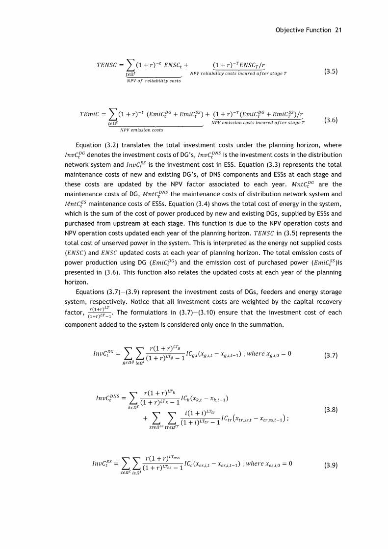
Equation (3.2) translates the total investment costs under the planning horizon, where

𝐼𝑛𝑣𝐶𝑡𝐷𝐺 denotes the investment costs of DG’s, 𝐼𝑛𝑣𝐶𝑡

𝐷𝑁𝑆 is the investment costs in the distribution

network system and 𝐼𝑛𝑣𝐶𝑡𝐸𝑆 is the investment cost in ESS. Equation (3.3) represents the total

maintenance costs of new and existing DG’s, of DNS components and ESSs at each stage and

these costs are updated by the NPV factor associated to each year. 𝑀𝑛𝑡𝐶𝑡𝐷𝐺 are the

maintenance costs of DG, 𝑀𝑛𝑡𝐶𝑡𝐷𝑁𝑆 the maintenance costs of distribution network system and

𝑀𝑛𝑡𝐶𝑡𝐸𝑆 maintenance costs of ESSs. Equation (3.4) shows the total cost of energy in the system,

which is the sum of the cost of power produced by new and existing DGs, supplied by ESSs and

purchased from upstream at each stage. This function is due to the NPV operation costs and

NPV operation costs updated each year of the planning horizon. 𝑇𝐸𝑁𝑆𝐶 in (3.5) represents the

total cost of unserved power in the system. This is interpreted as the energy not supplied costs

(𝐸𝑁𝑆𝐶) and 𝐸𝑁𝑆𝐶 updated costs at each year of planning horizon. The total emission costs of

power production using DG (𝐸𝑚𝑖𝐶𝑡𝐷𝐺) and the emission cost of purchased power (𝐸𝑚𝑖𝐶𝑡

𝑆𝑆)is

presented in (3.6). This function also relates the updated costs at each year of the planning

horizon.

Equations (3.7)—(3.9) represent the investment costs of DGs, feeders and energy storage

system, respectively. Notice that all investment costs are weighted by the capital recovery

factor, 𝑟(1+𝑟)𝐿𝑇

(1+𝑟)𝐿𝑇−1. The formulations in (3.7)—(3.10) ensure that the investment cost of each

component added to the system is considered only once in the summation.

𝐼𝑛𝑣𝐶𝑡𝐷𝐺 = ∑ ∑

𝑟(1 + 𝑟)𝐿𝑇𝑔

(1 + 𝑟)𝐿𝑇𝑔 − 1𝐼𝐶𝑔,𝑖(𝑥𝑔,𝑖,𝑡 − 𝑥𝑔,𝑖,𝑡−1)

𝑖𝜖𝛺𝑖𝑔𝜖𝛺𝑔

; 𝑤ℎ𝑒𝑟𝑒 𝑥𝑔,𝑖,0 = 0 (3.7)

𝐼𝑛𝑣𝐶𝑡𝐷𝑁𝑆 = ∑

𝑟(1 + 𝑟)𝐿𝑇𝑘

(1 + 𝑟)𝐿𝑇𝑘 − 1𝐼𝐶𝑘(𝑥𝑘,𝑡 − 𝑥𝑘,𝑡−1

𝑘𝜖𝛺ℓ

)

+ ∑ ∑𝑖(1 + 𝑖)𝐿𝑇𝑡𝑟

(1 + 𝑖)𝐿𝑇𝑡𝑟 − 1𝑡𝑟𝜖𝛺𝑡𝑟𝑠𝑠𝜖𝛺𝑠𝑠

𝐼𝐶𝑡𝑟(𝑥𝑡𝑟,𝑠𝑠,𝑡 − 𝑥𝑡𝑟,𝑠𝑠,𝑡−1) ;

(3.8)

𝐼𝑛𝑣𝐶𝑡𝐸𝑆 = ∑∑

𝑟(1 + 𝑟)𝐿𝑇𝑒𝑠𝑠

(1 + 𝑟)𝐿𝑇𝑒𝑠 − 1𝐼𝐶𝑐(𝑥𝑒𝑠,𝑖,𝑡 − 𝑥𝑒𝑠,𝑖,𝑡−1)

𝑖𝜖𝛺𝑖𝑐𝜖𝛺𝑐

; 𝑤ℎ𝑒𝑟𝑒 𝑥𝑒𝑠,𝑖,0 = 0 (3.9)

𝑇𝐸𝑁𝑆𝐶 = ∑(1 + 𝑟)−𝑡

𝑡𝜖Ω𝑡

𝐸𝑁𝑆𝐶𝑡⏟ 𝑁𝑃𝑉 𝑜𝑓 𝑟𝑒𝑙𝑖𝑎𝑏𝑖𝑙𝑖𝑡𝑦 𝑐𝑜𝑠𝑡𝑠

+ (1 + 𝑟)−𝑇𝐸𝑁𝑆𝐶𝑇/𝑟⏟ 𝑁𝑃𝑉 𝑟𝑒𝑙𝑖𝑎𝑏𝑖𝑙𝑖𝑡𝑦 𝑐𝑜𝑠𝑡𝑠 𝑖𝑛𝑐𝑢𝑟𝑒𝑑 𝑎𝑓𝑡𝑒𝑟 𝑠𝑡𝑎𝑔𝑒 𝑇

(3.5)

𝑇𝐸𝑚𝑖𝐶 = ∑(1 + 𝑟)−𝑡

𝑡𝜖Ω𝑡

(𝐸𝑚𝑖𝐶𝑡𝐷𝐺 + 𝐸𝑚𝑖𝐶𝑡

𝑆𝑆)⏟

𝑁𝑃𝑉 𝑒𝑚𝑖𝑠𝑠𝑖𝑜𝑛 𝑐𝑜𝑠𝑡𝑠

+ (1 + 𝑟)−𝑇(𝐸𝑚𝑖𝐶𝑇𝐷𝐺 + 𝐸𝑚𝑖𝐶𝑇

𝑆𝑆)/𝑟⏟ 𝑁𝑃𝑉 𝑒𝑚𝑖𝑠𝑠𝑖𝑜𝑛 𝑐𝑜𝑠𝑡𝑠 𝑖𝑛𝑐𝑢𝑟𝑒𝑑 𝑎𝑓𝑡𝑒𝑟 𝑠𝑡𝑎𝑔𝑒 𝑇

(3.6)

22 Problem Formulations-A Mixed Integer Linear Programming Approach

In (3.7), 𝐼𝐶𝑔,𝑖 represents the investment cost of DG, 𝑥𝑔,𝑖,𝑡 is the investment variables for DG.

LTg is the life time of DG. Equations (3.9) and (3.10) are also based on the same principle. In

(3.8), 𝐿𝑇𝑘 and 𝐿𝑇𝑡𝑟 are the lifetime of distribution lines and transformers, respectively. And, in

(3.9), 𝐼𝐶𝑘 and 𝐼𝐶𝑡𝑟 are the investment costs on distribution lines and transformers, respectively.

Equation (3.10) stands for the maintenance costs of new 𝑀𝐶𝑔𝑁 and existing DGs 𝑀𝐶𝑔

𝐸at each

time stage. The maintenance cost of a new/existing feeder is included only when its

corresponding investment/utilization variable is different from zero in (3.11). Equation (3.12)

is related to the maintenance costs at each stage of energy storage.

𝑀𝑛𝑡𝐶𝑡𝐷𝐺 = ∑ ∑𝑀𝐶𝑔

𝑁


𝑥𝑔,𝑖,𝑡 + ∑ ∑𝑀𝐶𝑔𝐸


𝑢𝑔,𝑖,𝑡 (3.10)

𝑀𝑛𝑡𝐶𝑡𝐷𝑁𝑆 = ∑ 𝑀𝐶𝑘

𝐸𝑘𝜖𝛺𝑒ℓ 𝑢𝑘,𝑡 + ∑ 𝑀𝐶𝑘

𝑁𝑥𝑘,𝑡𝑘𝜖𝛺𝑛ℓ +

∑ 𝑀𝐶𝑡𝑟𝐸

𝑡𝑟𝜖𝛺𝐸_𝑡𝑟

𝑢𝑡𝑟,𝑠𝑠,𝑡 + ∑ 𝑀𝐶𝑘𝑁𝑥𝑡𝑟,𝑠𝑠,𝑡

𝑡𝑟𝜖𝛺𝑁_𝑡𝑟

(3.11)

𝑀𝑛𝑡𝐶𝑡𝐸𝑆 = ∑∑𝑀𝐶𝑒𝑠𝑥𝑒𝑠,𝑖,𝑡

𝑖𝜖𝛺𝑖𝑐𝜖𝛺𝑐

(3.12)

The total cost of power produced by new and existing DGs is given by equation (3.13). Note

that these costs depend on the amount of power generated at each scenario, snapshot and

stage. Therefore, these costs represent the expected costs of operation. Similarly, equations

(3.14) and (3.15) respectively account for the expected costs of energy supplied by the energy

storage system, and that purchased from upstream (i.e. transmission grid).

𝐸𝐶𝑡𝐷𝐺 = ∑ 𝜌𝑠 ∑ 𝜋𝑤 ∑ ∑(𝑂𝐶𝑔,𝑖,𝑠,𝑤,𝑡

𝑁 𝑃𝑔,𝑖,𝑠,𝑤,𝑡𝑁


+ 𝑂𝐶𝑔,𝑖,𝑠,𝑤,𝑡𝐸

𝑤𝜖𝛺𝑤

𝑃𝑔,𝑖,𝑠,𝑤,𝑡𝐸 )

𝑠𝜖𝛺𝑠

(3.13)

𝐸𝐶𝑡𝐸𝑆 = ∑ 𝜌𝑠 ∑ 𝜋𝑤 ∑ 𝜆𝑠,𝑤,𝑡

𝑒𝑠 𝑃𝑒𝑠,𝑖,𝑠,𝑤,𝑡𝑑𝑐ℎ

𝑒𝑠∈𝛺𝑒𝑠𝑤𝜖𝛺𝑤𝑠𝜖𝛺𝑠

(3.14)

𝐸𝐶𝑡𝑆𝑆 = ∑ 𝜌𝑠 ∑ 𝜋𝑤 ∑ 𝜆𝑠,𝑤,𝑡

𝜍𝑃𝜍,𝑠,𝑤,𝑡𝑆𝑆

𝜍∈𝛺𝜍𝑤𝜖𝛺𝑤𝑠𝜖𝛺𝑠

(3.15)

The penalty for the unserved power, given by (3.16), is also dependent on the scenarios,

snapshots and time stages. Equation (3.16) therefore gives the expected cost of unserved

energy in the system.

Objective Function 23

𝐸𝑁𝑆𝐶𝑡 = ∑ 𝜌𝑠 ∑ ∑𝜋𝑤𝜐𝑠,𝑤,𝑡𝛿𝑖,𝑠,𝑤,𝑡𝑖𝜖𝛺𝑖𝑤𝜖𝛺𝑤𝑠𝜖𝛺𝑠

(3.16)

The expected emission costs of power generated by new and existing DGs are given by

(3.17)-(3.19), and that of energy purchased from the grid is calculated using (3.20). Note that,

for the sake of simplicity, a linear emission cost function is assumed here. In reality, the

emission cost function is highly nonlinear and nonconvex, as in [44].

𝐸𝑚𝑖𝐶𝑡𝐷𝐺 = 𝐸𝑚𝑖𝐶𝑡

𝑁 + 𝐸𝑚𝑖𝐶𝑡𝐸 (3.17)

𝐸𝑚𝑖𝐶𝑡𝑁 = ∑ 𝜌𝑠 ∑ 𝜋𝑤 ∑ ∑𝜆𝑠,𝑤,𝑡

𝐶𝑂2𝑒𝐸𝑅𝑔𝑁𝑃𝑔,𝑖,𝑠,𝑤,𝑡

𝑁

𝑖𝜖𝛺𝑖𝑔𝜖𝛺𝑔𝑤𝜖𝛺𝑤𝑠𝜖𝛺𝑠

(3.18)

𝐸𝑚𝑖𝐶𝑡𝐸 = ∑ 𝜌𝑠 ∑ 𝜋𝑤 ∑ ∑𝜆𝑠,𝑤,𝑡

𝐶𝑂2𝑒𝐸𝑅𝑔𝐸𝑃𝑔,𝑖,𝑠,𝑤,𝑡

𝐸

𝑖𝜖𝛺𝑖𝑔𝜖𝛺𝑔𝑤𝜖𝛺𝑤𝑠𝜖𝛺𝑠

(3.19)

𝐸𝑚𝑖𝐶𝑡𝑆𝑆 = ∑ 𝜌𝑠 ∑ 𝜋𝑤 ∑∑𝜆𝑠,𝑤,𝑡

𝐶𝑂2𝑒𝐸𝑅𝜍𝑆𝑆𝑃𝜍,𝑠,𝑤,𝑡

𝑆𝑆

𝑖𝜖𝛺𝑖𝜍𝜖𝛺𝜍𝑤𝜖𝛺𝑤𝑠𝜖𝛺𝑠

(3.20)

3.1.2 -Constraints

a) Kirchhoff’s current law (Active power balance)

The active power balance at each node is enforced by equation (3.21):

∑ (𝑃𝑔,𝑖,𝑠,𝑤,𝑡𝐸 + 𝑃𝑔,𝑖,𝑠,𝑤,𝑡

𝑁 )

𝑔𝜖Ω𝐷𝐺

+ ∑ (𝑃𝑒𝑠,𝑖,𝑠,𝑤,𝑡𝑑𝑐ℎ − 𝑃𝑒𝑠,𝑖,𝑠,𝑤,𝑡

𝑐ℎ )

𝑒𝑠𝜖Ω𝑒𝑠

+ 𝑃𝜍,𝑠,𝑤,𝑡𝑆𝑆 + ∑ 𝑃𝑘,𝑠,𝑤,𝑡

𝑖𝑛,𝑘𝜖𝑖

− ∑ 𝑃𝑘,𝑠,𝑤,𝑡𝑜𝑢𝑡,𝑘𝜖𝑖

+ 𝛿𝑖,𝑠,𝑤,𝑡

= ∑ 0.5𝜑𝑘,𝑠,𝑤,𝑡𝑖𝑛,𝑘𝜖𝑖

+ ∑ 0.5𝜑𝑘,𝑠,𝑤,𝑡𝑜𝑢𝑡,𝑘𝜖𝑖

+ 𝐷𝑠,𝑤,𝑡𝑖 ; ∀𝜍, ∀𝜍𝜖𝑖

(3.21)

Equation (3.21) denotes that the sum of all incoming flows should be equal to the sum of

all outgoing flows at each node. The losses in every feeder are considered as “virtual loads”

which are equally distributed between the nodes connecting the feeder Note that losses are a

quadratic function of flows (not shown here). Hence, they are linearized using first order

approximation, as in [68].

24 Problem Formulation – A mixed Integer Linear Programming Approach

b) Energy Storage Model Constraints

For the sake of simplicity, a generic ESS is employed here. This is modeled by the set of

constraints in (3.22)-(3.28). Equations (3.22) and (3.23) represent the bounds of power capacity

of the ESS while being charged and discharged, respectively. Inequality (3.24) prevents

simultaneous charging and discharging operation of ESS at the same operational time w. The

amount of stored energy within the ESS reservoir at a given operational time w as a function of

the energy stored until 𝑤 − 1 is given by (3.25). The maximum and minimum levels of storages

in the operational time w are also considered through inequality (3.26). Equation (3.27) shows

the initial level of stored energy in the ESS as a function of its maximum reservoir capacity. In

a multi-stage planning approach, Equation (3.28) ensures that the initial level of energy in the

ESS at a given year is equal to the final level of energy in the ESS in the preceding year. Here,

𝜂𝑒𝑠𝑑𝑐ℎ is assumed to be 1/𝜂𝑒𝑠

𝑐ℎ.

0 ≤ 𝑃𝑒𝑠,𝑖,𝑠,𝑤,𝑡𝑐ℎ ≤ 𝐼𝑒𝑠,𝑖,𝑠,𝑤,𝑡

𝑐ℎ 𝑥𝑒𝑠,𝑖,𝑡𝑃𝑒𝑠,𝑖𝑐ℎ,𝑚𝑎𝑥 (3.22)

0 ≤ 𝑃𝑒𝑠,𝑖,𝑠,𝑤,𝑡𝑑𝑐ℎ ≤ 𝐼𝑒𝑠,𝑖,𝑠,𝑤,𝑡

𝑐ℎ 𝑥𝑒𝑠,𝑖,𝑡𝑃𝑒𝑠,𝑖𝑐ℎ,𝑚𝑎𝑥 (3.23)

𝐼𝑒𝑠,𝑖,𝑠,𝑤,𝑡𝑐ℎ + 𝐼𝑒𝑠,𝑖,𝑠,𝑤,𝑡

𝑑𝑐ℎ ≤ 1 (3.24)

𝐸𝑒𝑠,𝑖,𝑠,𝑤,𝑡 = 𝐸𝑒𝑠,𝑖,𝑠,𝑤−1,𝑡 + 𝜂𝑐ℎ,𝑒𝑠𝑃𝑒𝑠,𝑖,𝑠,𝑤,𝑡𝑐ℎ − 𝜂𝑑𝑐ℎ,𝑒𝑠𝑃𝑒𝑠,𝑖,𝑠,𝑤,𝑡

𝑑𝑐ℎ (3.25)

𝐸𝑒𝑠,𝑖𝑚𝑖𝑛𝑥𝑒𝑠,𝑖,𝑡 ≤ 𝐸𝑒𝑠,𝑖,𝑠,𝑤,𝑡 ≤ 𝑥𝑒𝑠,𝑖,𝑡𝐸𝑒𝑠,𝑖

𝑚𝑎𝑥 (3.26)

𝐸𝑒𝑠,𝑖,𝑠,𝑤0,𝑇1 = 𝜇𝑒𝑠𝑥𝑒𝑠,𝑖,𝑇1𝐸𝑒𝑠,𝑖𝑚𝑎𝑥 (3.27)

𝐸𝑒𝑠,𝑖,𝑠,𝑤1,𝑡+1 = 𝐸𝑒𝑠,𝑖,𝑠,𝑊,𝑡 (3.28)

Inequalities (3.22) and (3.23) involve products of charging/discharging indicator variables

and investment variable. In order to linearize this, new continuous positive variables 𝑧𝑒𝑠,𝑖,𝑠,𝑤,𝑡𝑐ℎ ,

and 𝑧𝑒𝑠,𝑖,𝑠,𝑤,𝑡𝑑𝑐ℎ , which replaces the bilinear products in each constraint, is introduced such that

the set of linear constraints in (3.29) and (3.30) hold. For instance, the product 𝐼𝑒𝑠,𝑖,𝑠,𝑤,𝑡𝑑𝑐ℎ 𝑥𝑒𝑠,𝑖,𝑡 is

replaced by the positive variable 𝑧𝑒𝑠,𝑖,𝑠,𝑤,𝑡𝑑𝑐ℎ . Then, the bilinear product is decoupled by

introducing the set of constraints in (3.29) [69]. Similarly, the product 𝐼𝑒𝑠,𝑖,𝑠,𝑤,𝑡𝑐ℎ 𝑥𝑒𝑠,𝑖,𝑡is decoupled

by including the set of constraints (3.30).

Constraints 25

𝑧𝑒𝑠,𝑖,𝑠,𝑤,𝑡𝑑𝑐ℎ ≤ 𝑥𝑒𝑠

𝑚𝑎𝑥𝐼𝑒𝑠,𝑖,𝑠,𝑤,𝑡𝑑𝑐ℎ ; 𝑧𝑒𝑠,𝑖,𝑠,𝑤,𝑡

𝑑𝑐ℎ ≤ 𝑥𝑒𝑠,𝑖,𝑡 ; 𝑧𝑒𝑠,𝑖,𝑠,𝑤,𝑡𝑑𝑐ℎ ≥ 𝑥𝑒𝑠,𝑖,𝑡 − (1 − 𝐼𝑒𝑠,𝑖,𝑠,𝑤,𝑡

𝑑𝑐ℎ )𝑥𝑒𝑠𝑚𝑎𝑥 (3.29)

𝑧𝑒𝑠,𝑖,𝑠,𝑤,𝑡𝑐ℎ ≤ 𝑥𝑒𝑠

𝑚𝑎𝑥𝐼𝑒𝑠,𝑖,𝑠,𝑤,𝑡𝑐ℎ ; 𝑧𝑒𝑠,𝑖,𝑠,𝑤,𝑡

𝑐ℎ ≤ 𝑥𝑒𝑠,𝑖,𝑡 ; 𝑧𝑒𝑠,𝑖,𝑠,𝑤,𝑡𝑐ℎ ≥ 𝑥𝑒𝑠,𝑖,𝑡 − (1 − 𝐼𝑒𝑠,𝑖,𝑠,𝑤,𝑡

𝑐ℎ )𝑥𝑒𝑠𝑚𝑎𝑥 (3.30)

a) Active Power Limits of DGs

The active power limits of existing generators are given by (3.31). In the case of new

generators, the corresponding constraints are (3.32). Note that the binary variables multiply

both bounds to make sure that the power generation variable is zero when the generator

remains either unutilized or unselected for investment.

𝑃𝑔,𝑖,𝑠,𝑤,𝑡𝐸,𝑚𝑖𝑛 𝑢𝑔,𝑖,𝑡 ≤ 𝑃𝑔,𝑖,𝑠,𝑤,𝑡

𝐸 ≤ 𝑃𝑔,𝑖,𝑠,𝑤,𝑡𝐸,𝑚𝑎𝑥 𝑢𝑔,𝑖,𝑡 (3.31)

𝑃𝑔,𝑖,𝑠,𝑤,𝑡𝑁,𝑚𝑖𝑛 𝑥𝑔,𝑖,𝑡 ≤ 𝑃𝑔,𝑖,𝑠,𝑤,𝑡

𝑁 ≤ 𝑃𝑔,𝑖,𝑠,𝑤,𝑡𝑁,𝑚𝑎𝑥 𝑥𝑔,𝑖,𝑡 (3.32)

It should be noted that these constraints are applicable only for conventional DGs. In the

case of variable generation source (such as wind and solar PV), the upper bound 𝑃𝑔,𝑖,𝑠,𝑤,𝑡𝑚𝑎𝑥 should

be set equal to the minimum of the actual production level at a given hour, which is dependent

on the level of primary energy source (wind speed and solar radiation), and the rated (installed)

capacity of the generating unit. And, the lower bound 𝑃𝑔,𝑖,𝑠,𝑤,𝑡𝑚𝑎𝑥 in this case is simply set to zero.

b) Active Power Limits of Power Purchased

𝑃𝑠,𝑤,𝑡𝑆𝑆,𝑚𝑖𝑛 ≤ 𝑃𝑠,𝑤,𝑡

𝑆𝑆 ≤ 𝑃𝑠,𝑤,𝑡𝑆𝑆,𝑚𝑎𝑥 (3.33)

For technical reasons, the power that can be purchased from the transmission grid could

have minimum and maximum limits, which is enforced by (3.33). However, it is understood that

setting the maximum and minimum limits is difficult. These constraints are included here for

the sake of completeness. In this work, these limits are set to 1.5 times the minimum and

maximum levels of total load in the system.

c) Logical constraints

The set of logical constraints in (3.34) ensure that an investment decision cannot be

reversed. In addition to the constraints described above, the direct current (DC) based network

model and radiality related constraints presented in [68] are used here.


𝑥𝑘,𝑡 ≥ 𝑥𝑘,𝑡−1; 𝑥𝑔,𝑖,𝑡 ≥ 𝑥𝑔,𝑖,𝑡−1; 𝑥𝑒𝑠,𝑖,𝑡 ≥ 𝑥𝑒𝑠,𝑖,𝑡−1 (3.34)

d) Radiality constraints

There are two conditions that must be fulfilled in order a distribution network system (DNS)

to be radial. First, the solution must have 𝑁𝑖 − 𝑁𝑆𝑆 circuits. Second, the final topology should

be connected. Equation (3.35) represents the first necessary condition for maintaining the

radial topology of DNs.

∑ 𝑂𝑅(𝑥𝑘,𝑡 , 𝑢𝑘,𝑡)

𝑘∈Ω𝑖𝑗

= 𝑁𝑖 − 𝑁𝑆𝑆 ; ∀𝑡 (3.35)

Note that the above equation assumes line investment is possible in all corridors. Hence, in

a given corridor, we can have either an existing branch or a new one, or both connected in

parallel, depending on the economic benefits of the final setup (solution) brings about to the

system. The radiality constraint in (3.35) then has to accommodate this condition. One way to

do this is using the Boolean logic operation, as in (3.35). Unfortunately, this introduces

nonlinearity. We show how this logic can be linearized using an additional auxiliary variable

𝑧𝑘,𝑡 and the binary variables associated to existing and new branches i.e. 𝑢𝑘,𝑡 and 𝑥𝑘,𝑡, respectively. Given𝑧𝑘,𝑡: = 𝑂𝑅(𝑥𝑘,𝑡 , 𝑢𝑘,𝑡),this Boolean operation can be expressed using the

following set of linear constraints:

𝑧𝑘,𝑡 ≤ 𝑥𝑘,𝑡 + 𝑢𝑘,𝑡; 𝑧𝑘,𝑡 ≥ 𝑥𝑘,𝑡; 𝑧𝑘,𝑡 ≥ 𝑢𝑘,𝑡; 0 ≤ 𝑧𝑘,𝑡 ≤ 1 ; ∀𝑡 (3.36)

Then, the radiality constraints in (69) can be reformulated using the 𝑧𝑘,𝑡 variables as:

∑ 𝑧𝑘,𝑡𝑘∈𝛺𝑖𝑗

= 𝑁𝑖 − 𝑁𝑆𝑆 ; ∀𝑡 (3.37)

When all loads in the DNS are only fed by power from substations, the final solution obtained

automatically satisfies the two aforementioned conditions; hence, no additional constraints are

required i.e. (3.36) along with (3.37) are sufficient to guarantee radiality. However, it should

be noted that in the presence of DGs and reactive power sources, these constraints alone may

not ensure the radiality of the distribution network, as pointed out in [70] and further discussed

in [71].

3.2 – Summary

This chapter has presented a full description of the proposed dynamic and multi-objective

S-MILP model, which jointly takes into account the optimal RES-based DGs and DESS integration

in coordination with distribution network reinforcement and/or switching.

Summary 27

The problem has been formulated as with an objective of overall cost minimization. The

objective function is composed of Net Present Value (NPV) of five cost terms each weighted by

a certain relevance factor. The considered cost terms include the total investment cost, the

total cost of maintenance, consumed energy, unserved energy and emissions in the system all

under the assumption of perpetual planning horizon.

As already mentioned, in the formulation is employed one of the concepts most used in the

investment study in the financial world, the Net Present Value, which conceptually shows how

to value in monetary terms the cash flows in any investment planning, in this case, considering

the costs associated with the expansion planning of a given system.

This model will be tested in Chapter 5 on a case study and the further numerical results

will be discussed there.


29

Chapter 4

Problem Formulation and Solution -Genetic Algorithms Approach

In this chapter, a method to investigate the impacts of network switching as well as

installing DGs in distribution system is presented. To carry out this analysis, different models

are formulated. A brief description of the genetic algorithm employed is presented in this

chapter.

4.1 – An overview of Genetic Algorithms

Genetic algorithms are nature-inspired solution algorithms often suited for complex and

combinatorial problems [72] . Such algorithms are based on natural selection and genetic

mechanisms. They explore historic information to find points that are expected to lead to the

best performance. This is done by an iterative process. Each iteration is often referred to as a

generation. During each iteration, the principles of selection and reproduction are applied to

a population. The selection process determines the individuals that will be reproduced

(fathers), creating a determined number of descendants (sons) to the next generation by a

determined probability named fitness index. This can be understood as the individuals with

better relative adaptation, having greater chances to transmit their genes [73].

In a genetic algorithm, a possible population of solutions progresses according to the genetic

operators (probabilistic) conceived by biological representations. On average, there is a

tendency to have better solutions as the evolutionary process lasts. Notwithstanding, genetic

algorithm exploits a probabilistic and metaheuristic method to obtain new populations. It is not

a random solution search algorithm because it explores the available information to search new

individuals or better solutions to improve a performance index.

Genetic algorithms seek to privilege individuals with better skills. By this means, they try

to drive to regions of search space where global optima are located. Sometimes, this cannot be

achieved if the parameters are not well suited for the problem.

30 Problem Formulation and Solution -Genetic Algorithms Approach

4.1.1 -Codification

The basis to a genetic algorithm application to a problem is the representation of the

problem to be analyzed. Each representation must have matching genetic operators. This is

critical for genetic algorithms to operate correctly to the correspondingly optimization

problem.

Genetic algorithm creates populations of individuals. This is called a chromosome, a data

structure. Generally, chromosomes are vectors or binary values chain, reals or combinations of

both. A chromosome represents a possible solution to the problem. Hence, a chromosome forms

the set of parameters of the objective function that will be optimized. All the configurations

that a chromosome can assume is called a search space. If a chromosome has n parameters of

a function, it will be a search space with n dimensions. The majority of representations are

genotypic Genotype is the set of genes that defines the genetic constitution of an individual.

Genetic operators will be applied to genes [72]. Genotypes are represented by finite scale

vectors, that the user needs to specify (see in Figure 4.1).

The genotype of an individual is conventionally represented by a binary vector. Each

element of the vector characterizes a certain characteristic relevant to the construction of a

unique individual. Combinations of elements can form the real characteristics of an individual,

namely its phenotype. This representation is problem independent because once found the

representation in binary vectors, standard operations can be applied, helping the employing in

different classes of problems. Binary representation is the most commonly used approach

because it is easy to implement, manipulate and analyze. But if the problem has continuous

parameters, chromosomes could have bigger representations if the user wants to work with a

higher precision. This leads to the use of a larger amount of memory. The majority of genetic

algorithms proposed in the literature have a fixed number of individuals in a population, with

constant size chromosomes. This is the simplest method to create a population of individuals

[73].

Figure 4 Possible chromosome representation

.Figure 4.1 – Possible chromosome representation.

Initialization 31

Having defined the chromosomic representation to the problem, a possible set of solutions

are generated called aspirants. These aspirants are normally called sons due to the fact that

they have a genetic material from their fathers. The set of codified solutions according the

selected representation matches a population of individuals representing, over the evolution

cycles, the current stage of problem solution. In each iteration, the population is modified

because genetic algorithms involve an iterative process. Each iteration is called a generation

although not all population individuals are necessarily sons of individuals of the population in

the preceding iteration.

In the populations, several statistical values are calculated that will be used to evaluate if

the search is close to the optimal solution. Parameters that can be evaluated are the best

individual, diversity, standard deviation and average of accomplished goals. Normally, the

evaluation is done to the objective function, this is the simplest way. This is simply to say that

objective function becomes the fitness function, and there is no need to calculate the relative

fitness function.

4.1.2 -Initialization

The representation of a search space is the most sensitive issue. Hence, initialization leads

to some mechanism of making educated guess. The types of initializations are the following

[74]:

Random initialization – Individuals of the population are generated randomly.

Deterministic initialization – Individuals of the population are generated

deterministically by heuristic methods.

Random initialization with niche – Individuals of the population are generated by

ways that can be divided in species. This will group individuals with similar

characteristics.

Randomly initializing population of n individuals are generated or some heuristic methods

are used. This is the classic initialization that can be found in most relevant works. Without

variety, there is no evolution. The natural selection theory (Darwin’s Theory of Evolution)

implies individuals that have different adaptation index to the ambient where they live, so it

is important to have a large search space in the genetic algorithm.

Initial population generation can be obtained obeying some conditions established by the

user. The user can establish such conditions from previous knowledge of the problem. The more

restrictive these conditions are, the faster the convergence is. This is because the generated

values are closer to the desired (possibly optimal) solution. There is no formula to the number

of individuals that compose the population. They can be dependent on some heuristics but it’s

more reliant on the user’s experience, and his/her previous knowledge of the objective

function. The larger the number of individuals is, the higher the probability of convergence

because the probability of the solution among the elements of population is bigger. But this

may lead to greater computational effort, increasing the computation time. If the population

is too small, it will not have diversity, the search space is reduced and the convergence will be

premature.


32

The objective is to generate a population within a certain interval where it could be the

solution. With this, it is not necessary to generate a random population. In the current work,

we know that the number of branches must be equal to the number of buses minus the number

of generators to keep radial configuration of the DNS, consequently, we can generate a uniform

distribution between this fixed number of branches and zero.

4.1.3 -Evaluation

A genetic algorithm needs information about the value of the objective function to each

individual of the population. The objective function gives the measure of how good the

individual is adapted to the environment. In other words, this relates to the probability to

survive and reproduce, transferring its genetic material to the next generations. The evaluation

of the individual results in the so called “fitness function”[74].

Validating is the next step and it can be defined as the process to compare the fitness

function from all individuals and sorting them out by their corresponding fitness function

values. Normally, the best/bests are selected, according to the evolution theory. Convergence

and the performance of the population related to the objective function is analyzed. This can

be done by calculating the maximum, minimum and average of the fitness function or the

standard deviation in each generation. Convergence can be a process of setting a finite number

of generations (the most practical way).

If the initial population happens to have the exact solution to the problem, the algorithm

will not stop. Convergence of the algorithm is achieved only, for instance, when the average

fitness of the population is well stabilized or we reach the maximum number of generations.

This can indicate that the population is adapted to the environment and the elements lead to

the best objective function value. This can also indicate that we are stuck in an optimum

location and need to improve the search space. The best individual is saved whether it belongs

to the actual population or not. In the end, this will be the expected result. The recording is

always done in each generation to see if we reached the optimum solution.

In genetic algorithms, convergence can be very fast to a sub-optimal solution. This is not

what is desired, however. This problem is called premature convergence and it can occur by a

small population or badly distribution of initial population. Premature convergence can occur

due to bad distribution of individuals in search space and will affect the search for the global

optimum. Such a premature convergence is also called diversity loss. Diversity indicates the

rate which each region is represented in the solution search space. This can be overcome by

improving the distribution of individuals in the initial population and preventing loss of diversity

in the first generations. In addition, increasing the number of individuals will improve the

search space. The selection process will guarantee that the best individual will dominate the

next generation and so on if there are no better individuals with a best fitness function.

4.1.4 -Selection

Selection is the process that will make the initial population more fit after many

generations. This is the basic principle of genetic algorithms. Selection mechanism in genetic

algorithms tries to imitate the natural selection process [73], [74].

Selection 33

Genetic algorithms start with an initial population with a set of individuals. If we know a

priori where the solution is located, the first individuals can be initialized deterministically.

When we do not know anything about the search space, the individuals are created randomly.

Deterministic way can lead us to fast convergence because the global optimum can be in the

first generation. The selection process favors the fit individuals, and to a fitness function is

assigned to each individual. This function is an input that represents the genes of the

chromosome and provides their fitness as an outcome. Fitness is like a grade where the

evaluation is made by a solution coded from each individual. This fitness is based on the

objective function.

A relative fitness can be calculated to each individual. To some selection methods, it is

desirable that the value of relative fitness for each individual be less than 1 and that the sum

of every fitness values are equal to 1. The relative fitness of each individual is calculated by

dividing its value of fitness (objective function that the solution from the individual) by the

sum of values of the fitness of the entire individuals of the population (the sum of the objective

functions of each individual). This is expressed by equation (4.1).

𝑓(𝑥𝑖)𝑟𝑒𝑙 = 𝑓(𝑥𝑖)

∑ 𝑓(𝑥𝑗)𝑛𝑗=1

(4.1)

where 𝑓(𝑥𝑖) is the fitness function.

Generally, a population of n individuals is generated with a probability proportional to its

relative fitness in the population. Using the previous probability, we select n individuals.

Individuals with low fitness will have high probability to disappear from the population.

Individuals with high fitness will be passed on to the next generation. It is not necessary to

calculate this fitness function because when we have a fixed maximum generation, we can

analyze the objective function of each individual and select the best. This fitness function is a

good instrument when we have convergence by some other method than a fixed number of

generations (like average fitness of the population is well stabilized).

The objective function gives information about how close or far the solution is from the

desired solution. It includes restrictions that need to be satisfied by the solution. In

optimization problems, the objective function can be maximization or minimization of the

objective function. It can be maximization of profit or minimization of costs. Some problems

can include more than one objective function. Problems called multi-objective optimization

can have an objective function that includes more than one objective.

The selection process chooses a subassembly of individuals based on fitness, creating an

intermediate population. Different selection methods are implemented in genetic algorithms.

Most of all seek to favor the fittest individuals in order to keep population diversity. Some

methods are:

Roulette;

Tournament;

Stochastic sampling;

Classification.


The Roulette method is the simplest and the most commonly used approach. Individuals of

the generation are selected to the next generation using roulette as we see in the famous game

of casinos roulette wheel. Each individual is represented in the roulette according to their

fitness value. This way, individuals with nice fitness get a bigger interval in the roulette and

the others with low fitness will receive a shorter interval. After distribution in the roulette,

certain values are randomly generated in the interval from 0 to the total summary of the fitness

of all individuals, a determined number of times depending on the size of population. If a given

individual is in the interval, the generated value will be selected to the intermediate

population.

In tournament selection, n individuals of population are selected randomly with the same

probability. The individual with the greatest fitness among them is selected to the intermediate

population. Process ends when the intermediate population is fulfilled.

A stochastic sampling is a variation of Roulette method but instead of one unique needle,

n needles equally spaced are used, where n is the number of individuals to be selected. This

way, instead of spinning the roulette n times, it is only spinned one time.

A classification method primary classifies the population, then, each individual gets a grade

according to the classification of the population. The worst individual will get the lower value

that we can assign, the second worst gets the second worst value and successively. The best

will get the highest grade, that can be equal to the number of individuals in the population.

After the classification process, every individual has a certain chance to be selected.

4.1.5 -Genetic Operators

Global optimization algorithm must be capable of exploring new points inside the solution

search space. This mechanism is called exploration and exploitation, and is often adopted in

genetic algorithms by applying correct genetic operators. The main genetic operators are

crossover and mutation primarily in a binary codification [75].

Crossover uses information in two or more individuals (fathers) to generate one or more

individuals (sons). This can be resistant to add new information to population because it sees

the region close to father’s individuals. The process of recombination is a sexual process – it is

more than one individual – and stimulates the exchange of information between chromosome

pairs. It is a random process with a fixed probability that needs to be specified by the user.

Mutation can be a diversifier or booster to the solution search. Some approaches use

mutation as the technique responsible for the evolution process, for determining if the

movement is exploration or exploitation, and the adaptable parameters in each generation.

Mutation can diversify when new information is introduced in the individual, and consequently

to the population (very strong mutation). If the mutation is very weak, it is a booster in neighbor

solution search. This process is equivalent to the random search. One position is selected in the

chromosome, and changes the correspondent value to another random one. This can be

controlled with a fixed parameter that indicates the probability of a gene suffering mutation.

Crossover and mutation can be combined to upgrade the search for the optimal solution by

taking advantages of the best features in each method.

Genetic Algorithms: Formulation 35

4.1.6 -Genetic Parameters

The performance of a genetic algorithm is strongly dependent on how the parameters to be

employed are defined. Hence, it is important to investigate which way some parameters can

influence in the behavior of the algorithm [76]. This way, we can establish the parameters

according to the requirements and resources available. Parameters usually are size of

population, crossover rate, mutation rate, substitution rate and convergence condition. Size of

the population affects the global performance and efficiency of genetic algorithms. With a

small population, the performance may drop because a relatively small search space is covered.

Bigger population offers a representative search space domain and avoids optimum local

solutions. However, to work with bigger populations, we may need a longer simulation time or

more computation resources.

Crossover rate specifies how fast new structures are introduced in the population. If it is

set very high, good structures can be removed faster than the selection capacity. With a small

rate, the algorithm can become slow or stagnate. Mutation rate prevents that the search

becomes stagnated in regions of search space. It allows that every space search point can be

achieved. With a high rate, the search becomes random.

Substitution rate controls the population percentage that will be substituted in the next

generation. With a higher rate value, most of the population will be substituted but it can suffer

of losing great structures of fitness. When the rate value is too low, the algorithm may become

slow. Substitution rate is not commonly used because with a nice mutation and crossover rate,

we can guarantee that the next generations will be always better than the previous ones.

A convergence condition is the condition when the algorithm will stop. The ideal is to stop

when we reach the optimum solution in an optimization problem. When we have multimodal

functions (saddle points, with many optimal points and one global optimum) it can be sufficient

when we reach one optimal point but there are situations where the largest possible number

of optimal points is desired. In practical, we cannot tell with certain if a given point matches

the global optimum. As a consequence, it’s used as convergence condition a maximum number

of generations or a limit of computational time to stop the algorithm. Another criterion is to

stop the algorithm if during several generations the fitness function is not getting better,

interpreted as an idea of stagnation of the solution.

4.2 – Genetic Algorithms: Formulation

In this work, a GA is used to solve the resulting problems based on AC OPF models. The OPF

problems are solved using the MatPower toolbox in MATLAB environment. MatPower is a

package of MATLAB for solving power flow and optimal power flow problems. It is intended as

a simulation tool for researchers and educators that is easy to use and modify.

A GA is a method for solving constrained and unconstrained problems optimization

problems, particularly suited for non-linear and combinatorial problems. It is based on natural

selection. The process that guides a GA is basically initialization, mutation, evaluation and

selection. In this work, a GA is employed to solve the reconfiguration of distribution system as

wells as placement and sizing of DGs. The implementation process of the GA is summarized as

follows:


A GA is a method for solving constrained and unconstrained problems optimization

problems, particularly suited for non-linear and combinatorial problems. It is based on natural

selection. The process that guides a GA is basically initialization, mutation, evaluation and

selection. In this work, a GA is employed to solve the reconfiguration of distribution system as

wells as placement and sizing of DGs. The implementation process of the GA is summarized as

follows:

Step 1: Initialization – Generate the set of branches and set of DG’s in each node

Step 2: Mutation – Mutate the chromosome of branches and DG’s

Step 3: Evaluation - Check the radially constraints

Step 4: Run the OPF of radial populations

Step 5: Selection

Step 6: Uniform Crossover and a Small Mutation - Crossover and Small mutation for

a new population based on the best populations.

Step 7: Selection – Select the best population.

The chromosome of the set of branches connected is binary, 1 if connected and 0 if

disconnected. The generation of radial populations is based on number of buses minus the

number of generators. The DG placement does not affect this stipulation. The algorithm used

is shown in Figure 4.2.

The DG chromosome is generated by integer numbers between 0 and 4, respecting the size

of DG in MW and with a length of number of buses. This way we generate the location and size

of DG. The parameters of the network are introduced in a MatPower case. To solve the OPF,

we just need to pass to the MatPower information regarding the statuses of the branches.

The DGs are regarded as a PV bus. Hence, in order to solve the OPF, we need to introduce

the generator data and the generator cost data. Running the OPF, we obtain the voltage profile,

costs and line flows.

First, we will investigate the benefits of having only reconfiguration in the system. Second,

we will solve the problem of DG placement and sizing along with the reconfiguration problem.

This way, the best places to install DG’s and their optimal size, as well the network topology is

determined.

The objective function is the total costs in the system. This will be our fitness function that

needs to be minimized.

In order to get the best topology, we penalize the configurations that do not lead to radial

configurations. Then, if it fulfils the radially constraints, we check if all buses are connected.

If not, another penalization is introduced. After running the OPF and see if it converges,

investigation regarding voltage limits is done. If the voltage limits are not respected, another

penalization is introduced in the fitness function. If the OPF does not converge, we penalize

the fitness. This will lead to the best cases.

This process is also reproduced when we introduce DGs in the problem. A DG is treated as

another population and all the constraints regarding the OPF will be checked and respected.

Different costs of DG are considered in order to seek for the best cases.

Genetic Algorithms: Formulation 37

Figure 5 Flow Chart of the proposed GA.

.Figure 4.2 – Flow Chart of the proposed GA.


4.3 – Summary

In this chapter, an overview of the genetic algorithm (GA), the optimization problems and

the solution procedures have been described. Overall, the problem considered in the

optimization process jointly takes into account the optimal DGs placement and size in

coordination with distribution network switching in one operation scenario.

The resulting problem has been solved using a genetic algorithm, where a brute-force AC

OPF is considered with an objective of overall cost minimization. The objective function is

composed of costs related to power production in one operation scenario. In addition, loss

minimization has been taken into consideration with reconfiguration of the distribution system.

39

Chapter 5

Case Studies, Results and Discussion

5.1 – Mixed Integer Linear Programming based Optimization

5.1.1 – Case Study: A 33-bus Test System

A standard IEEE 33-bus radial distribution network, shown in Figure 5.1, is used here for

carrying out the required analysis mentioned earlier. The system has a rated voltage of 12.66

kV, and a total demand of 3.715 MW and 2.3 MVAr. Network data and other related information

about this test system can be found in [77]. Other data and assumptions made throughout this

paper are as follows:

The planning horizon is 3 years long, which is divided into yearly planning stages, and

a fixed interest rate of 7% is used.

The expected lifetime of ESS is assumed to be 15 years while that of DGs and feeders

is 25 years.

Two investment options with installed capacities of 0.5 and 1.0 MVA are considered for

each wind and solar PV type DG units.

The installation cost and emission related data of these DG units, provided in [78], are

used here.

For the sake of simplicity, all maintenance costs of DGs are assumed to be 2% of the

corresponding investment costs while that of feeders is 450 €/km/year.

The investment cost of each feeder is 38700 €/km.

The current limits of all feeders is assumed to be 200 A except for those between nodes

1 and 9 which is 400 A.

It is assumed that all feeders can be switched on/off, if deemed necessary

In addition, it is assumed that wind and solar power sources are uniformly available at

every node.

The cost of energy storage is 1000k€/MW;

40 Case Studies, Results and Discussion

The operational variability and uncertainty introduced by wind and solar PV type DGs,

demand and electricity price are accounted for via the clustering method proposed in

[79].

The maximum allowable bus voltage deviation in the system is set to 5%, and node 1 is

considered as a reference with a voltage magnitude of 1.0. Annual demand growths of

0%, 5% and 10% are also considered in all simulations.

Emission prices in the first, second and third stages are set to 25, 45 and 60 €/tCO2e,

respectively, and the emission rate of power purchased from upstream is arbitrarily set

to 0.4 tCO2e/MWh.

The cost of unserved energy is 2000 €/MWh. A power factor of 0.9 is considered in the

system, and is assumed to be the same throughout. The base power is set to 1 MVA.

The computed values of relevant variables are analyzed for different cases (as depicted in

Table 5.1) over the three years planning horizon. Case 1 represents the base case topology

where no investments are made while Case 2 considers an optimal reconfiguration but with no

investments. Cases 3 and 4 both consider investments in DGs only but differ in that the former

does not change the network topology and the latter uses optimal switching. The last two cases

correspond to scenarios where investments in DGs are coordinated with that of ESSs. Case 5

uses the topology in the base-case while Case 6 uses network reconfiguration.

5.1.2 – Results and Discussion

The results in Table 5.1 reveal the significant differences in overall NPV cost in the system,

share of energy supplied by RES and ESS combined, cost of total network losses and unserved

power among the aforementioned cases. The results are also compared with the base case

system where no investments are made and the network topology is held the same. Network

reconfiguration alone, as in Case 2, results in about 8.4% in the cost of losses, and a 3.1%

reduction in the NPV overall system cost compared with that of Case 1. In addition, network

reconfiguration avoids a total of 396.3 kVA load curtailment (or 256.9 kVA in Case 3) that would

otherwise occur at nodes 17, 18, 32 and 33 due to voltage limit constraints in

Case 1.

Figure 6 - 33-bus radial distribution system.

Figure 5.1 - 33-bus radial distribution system.

1 2 3

19

26

23 24 25

4 5 6 7 8 9 10 11 12 13 14 15 16 17 18

20 21 22

27 28 29 30 31 32 33

Results and Discussion 41

Another more interesting observation from Table 5.1 is that Cases 3 and 4 result in

(approximately) 60% reductions in the overall cost of the system and the amount of imported

energy. Wind and solar power sources are complementary by nature. This important

phenomenon seems to be exploited when DG investments are not accompanied by investments

in ESSs (i.e. Cases 3 and 4). This is because, according to the DG investment solution in Table

5.1, the operational variability in the system seems to be handled by investing an appreciable

amount in both complementary power sources (wind and solar). This can also be seen from the

level of demand covered by RESs, which is about 58%.

The results corresponding to Cases 5 and 6 show that the total cost and cost of losses are

dramatically reduced by more than 41.6% and 80% respectively. This reveals the substantial

benefits of coordinating investments DG with ESSs. Generally, ESSs significantly improve system

flexibility, enabling large-scale accommodation RES energy. Interestingly, the total amount of

installed DGs (9 MW) is the same for Cases 3—6 i.e. with/without ESSs. Even if this is the case,

in the absence of ESSs (Cases 3 and 4), there may be spillage of RES power when the demand

is lower than the total generated power. However, the installation of ESSs leads to an efficient

utilization of RES power. This is evident from the amount of energy consumption covered by

the combined energy supplied by RESs and ESSs in Cases 5 and 6 is about 89%.

Normally, network switching capability also improves system flexibility, leading to a high

level RES penetration. In this particular study, the effect of network switching on the level of

RES power absorbed by the system is not significant as one can observe in Table 5.1. This may

however be case-dependent. A more frequent switching capability could, for instance, have

significant impact.

The optimal location and size of installed DGs corresponding to Cases 3 through 6 is shown

in Figure 5.2. The average voltage profiles at each node and for each case are depicted in

Figure 5.3. It is interesting to see in this figure the substantial contributions of DGs and ESS

installations to voltage profile improvement.

As shown in Figure 5.3, the coordinated integration of DGs and ESSs (i.e. Case 6), especially

leads to the best voltage profile. Figure 5.4 demonstrates the optimal network topology, DG

and ESS locations corresponding to this case. The nodes 8, 14, 25, 30 and 32 are within the 4

cases. We can assume that these nodes possibly are the critical nodes to invest. The benefit of

joint DG and ESS investments along with network reconfiguration in terms of losses reduction

(over 84% on average) can be seen from figure 5.5. The spikes observed in Case 6 are because

of the variability in RES power injected into the system.

Table 5.1 - Results of Relevant Variables for Different Cases. Table 1 - Re sults of Relevant Variab les for Dif ferent Cases.

Cases Total cost

(TC) [k€]

Energy supplied by

RES and ESS [%]

Total cost of

losses [k€]

Total cost of

unserved power

[k€]

Total installed

size [p.u.]

Wind Solar ESS

1 45447.91 0.0 1089.80 1505.70 0.0 0.0 0.0

2 44044.58 0.0 997.85 0.00 0.0 0.0 0.0

3 33281.50 58.1 433.58 161.79 6.0 3.0 0.0

4 33106.07 58.2 404.59 0.00 6.0 3.0 0.0

5 26522.10 88.8 218.33 0.00 8.0 1.0 3.0

6 26516.52 88.8 212.73 0.00 8.0 1.0 3.0

Figure 7 - Optimal DG location in Cases 3, 4, 5 and 6. Table 2 - Resu lts of Re levant Variable s fo r Different Cases.


Figure 10 - Average voltage prof iles in the system under d ifferent cases.

Figure 11 - Average voltage profiles in the system under different cases.

Figure 5.3 - Average voltage profiles in the system under different cases.

Figure 12 - Optimal locations of DGs and ESSs under Case 6 (Opened switches 28-29, 8-21, 9-1

5, 18-33, 12-22).

Figure 5.4 - Optimal locations of DGs and ESSs under Case 6 (Opened switches 28-29, 8-21, 9-15, 18-33, 12-22).

0,94

0,95

0,96

0,97

0,98

0,99

1

1,01

N1 N3 N5 N7 N9 N11 N13 N15 N17 N19 N21 N23 N25 N27 N29 N31 N33

Volt

age (

pu)

Nodes

Case 1 Case 2 Case 3

Case 4 Case 5 Case 6

1 2 3

19

26

23 24 25

4 5 6 7 8 9 10 11 12 13 14 15 16 17 18

20 21 22

27 28 29 30 31 32 33

Wind

Solar

ESS

W

S

W W

W W

W W

S

W

0

0,5

1

1,5

2

2,5

N4 N7 N8 N14 N18 N20 N23 N24 N25 N30 N32

Siz

e o

f D

G inst

alled (

MVA)

Optimal DG location (nodes)

Case 3 Case 4 Case 5 Case 6

Figure 8 - Optimal DG location in Cases 3, 4, 5 and 6.

Figure 9 - Optimal DG location in Cases 3, 4, 5 and 6. Figure 5.2 - Optimal DG location in Cases 3, 4, 5 and 6.

Genetic Algorithm Results 43

As shown in Figure 5.3, the coordinated integration of DGs and ESSs (i.e. Case 6), especially

leads to the best voltage profile. Figure 5.4 demonstrates the optimal network topology, DG

and ESS locations corresponding to this case. The nodes 8, 14, 25, 30 and 32 are within the 4

cases. We can assume that these nodes possibly are the critical nodes to invest. The benefit of

joint DG and ESS investments along with network reconfiguration in terms of losses reduction

(over 84% on average) can be seen from figure 5.5. The spikes observed in Case 6 are because

of the variability in RES power injected into the system.

5.2 – Genetic Algorithm Results

5.2.1 – Case Study: 16-bus Test System

Figure 5.6 shows the 16-bus test system used for analysis of the results from GA. The system

has a rated voltage of 23 kV and a total demand of 28.7 MW and 17.3 Mvar. The maximum

allowable bus voltage deviation in the system is set to 5%. A power factor of 0.95 is considered

for the DG. The costs of the generators at the feeders are given by polynomial functions, and

two options are considered as in (5.1) and (5.2):

𝐶(𝑃) = 150 + 20𝑃 + 0.01𝑃2 €/h (5.1)

𝐶(𝑃) = 180 + 30𝑃 + 0.03𝑃2 €/h (5.2)

For integrating the DG as a PV bus and add to the cost of the system given by the OPF, one

polynomial function (5.3) was taken in consideration.

Figure 13 - Total system losses profile. Figure 5.5 - Total system losses profile.

0

0,02

0,04

0,06

0,08

0,1

0,12

0,14

1 5 9

13

17

21

25

29

33

37

41

45

49

53

57

61

65

69

73

77

81

85

89

93

97

101

105

Loss

es

(p.u

.)

Operational snapshots

Case 6 Case 1


𝐶(𝑃) = 8𝑃 €/h (5.3)

It is assumed that DG power sources are uniformly available at every node. Nodes 1, 2 and

3 are considered as references. The base power is set to 1 MVA. Network data and other related

information about this test system can be found in [80]. The variations of different relevant

parameters when considering different cases (as depicted in Table 5.2) are analyzed.

Case 1 represents the base case with the 3 feeders having the same costs

Case 2 considers reconfiguration of the base case

Case 3 refers to the base case reconfiguration but with different generation costs

at the feeders

Case 4 considers reconfiguration with different costs for feeders;

Cases 5 and 6 denote scenarios where, instead of minimization of costs, we

minimize the losses but they differ in the costs of feeders that are different in Case

6

Case 7 considers the reconfiguration with DG capable of injecting and absorbing

active and reactive power

Case 8 considers reconfiguration with DG capable of injecting and absorbing active

power

Case 9 considers reconfiguration with DG capable of injecting and absorbing

reactive power

In Cases 3, 4 and 6, three scenarios for different costs are proposed: 1) the generator at

feeder 1 (F1) is more expensive, 2) the generator at feeder 2 (F2) is more expensive, 3) the

generator at feeder 3 (F3) is more expensive.

Figure 14 - 16-bus radial distribution system [67]. Figure 5.6 - 16-bus radial distribution system [67].

Figure 15 - 16-bus radial distribution system [67]. Figure 5.6 - 16-bus radial distribution system [67].

Feeder I Feeder II Feeder III

1 2 3

4

5

6 7

8

910

11

12

13

14

1516

L 1

L 2

L 3

L 4

L 5

L 6

L 7

L 8

L 9

L 10

L 11

L 12

L 13

L 14

L 15L 16

Results and Discussion of the 16-bus Test System 45

5.2.2 – Results and Discussion of the 16-bus Test System

The results in Table 5.2 reveal significant differences in overall operation costs, active and

reactive power losses and total installed size of DGs. Network reconfiguration, Case 2,

compared with base case, Case 1, results in about 0.04% of reduction in total cost, a 7.17%

reduction in total active power losses and a 5.98% reduction in total reactive power losses.

Topology from Case 2 is shown in figure 5.7. The voltage profile can be seen in Figure 5.8. The

improvement in voltage profile is appreciable. Table 5.3 summarizes the numerical results

concerning the network topology (opened branches) along with the DG location and size.

Comparing the costs corresponding to different generation cost assumptions at the feeders, i.e.

Case 4 with Case 3, there are some relevant issues worth mentioning here. The first one is that

the costs are lower in Case 4 than in Case 3, but we get higher values of losses. This may be

due to the fact that the reconfiguration tries to find the path that minimizes the involvement

of the more expensive feeder. We can see in Figure 5.9 that the feeder is always with one bus,

feeding the demand. We will get a feeder that will be feeding more buses and the losses will

increase comparing the cases that are related. All the scenarios in Case 6 have the same

configuration, that is the same configuration of the Case 2. This configuration is illustrated in

Figure 5.7. In addition, in Case 6, the scenarios seem to lead to high total costs except in 6-F2.

This shows that the single reconfiguration of the system is different if we are considering

minimization of losses or minimization of costs.

In Figure 5.10, we see that the voltage profile for case 4-F2 is worse than the case 3-F2

despite having obtained the best costs in case 4-F2. This is because the topology of

the network that leads to bigger losses, impacting the voltage profiles. The voltage profiles

of Case 6 are the same as Case 2, and Figure 5.8 reveals this phenomenon.

Table 5.2 – Results of Relevant Variables for Different Cases. Table 3 - Rele vant Variable s Re sults fo r Diffe rent Case s.

Cases Total Cost

[€/h]

Total Active

Power Losses

[MW]

Total Reactive

Power Losses

[Mvar]

Total

installed DG

size [MVA]

Computation

time [s]

1 1029.4177 0.1064 0.1224 0 -

2 1029.0201 0.0987 0.1151 0 7.848185

3-F1 1146.0389 0.1064 0.1224 0 -

3-F2 1215.8225 0.1064 0.1224 0 -

3-F3 1111.0366 0.1064 0.1224 0 -

4-F1 1081.0391 0.1510 0.1680 0 8.262878

4-F2 1100.7268 0.1480 0.1777 0 12.175396

4-F3 1070.4623 0.1251 0.1517 0 9.956841

5 1029.0201 0.0987 0.1151 0 7.540224

6-F1 1151.8748 0.0987 0.1151 0 6.644372

6-F2 1198.3556 0.0987 0.1151 0 11.134548

6-F3 1120.9084 0.0987 0.1151 0 9.013040

7 790.0860 0.0290 0.0311 21 24.246142

8 790.0860 0.0540 0.0583 16 30.989449

9 1028.8530 0.0927 0.1054 14 27.035288

Table 4 Relevant Variable Results for Different Cases


Table 5.3 - Opened Branches and Location of DG. Table 53 - Opened Branches and Location of DG.

Cases Opened branches DG Bus Location

1 5-11; 10-14; 7-16 -

2 8-10; 9-11; 7-16 -

3-F1 5-11; 10-14; 7-16 -

3-F2 5-11; 10-14; 7-16 -

3-F3 5-11; 10-14; 7-16 -

4-F1 4-5; 4-6; 8-10 -

4-F2 4-6; 8-9; 8-10 -

4-F3 9-11; 13-14; 13-15 -

5 8-10; 9-11; 7-16 -

6-F1 8-10; 9-11; 7-16 -

6-F2 8-10; 9-11; 7-16 -

6-F3 8-10; 9-11; 7-16 -

7 6-7; 9-11; 10-14 4; 5; 6; 7; 9 12; 15

8 6-7; 13-14; 5-11 5; 6; 11; 12; 13; 15

9 6-7; 8-10; 9-11 4; 6; 9; 15; 16

Figure 16 - New topology of the distribution system from Case 2.

Figure 5.7 - New topology of the distribution system from Case 2.

Figure 17 - Voltage comparison between base case and reconfiguration. Figure 5.8 - Voltage comparison between base case and reconfiguration.


1 2 3

4

5

6 7

8

910

11

12

13

14

1516

L 1

L 2

L 3

L 4

L 5

L 6

L 8

L 10

L 11

L 12

L 15

L 14

L 13

0,94

0,95

0,96

0,97

0,98

0,99

1

1,01

1,02

1,03

1,04

1,05

1,06

1 2 3 4 5 6 7 8 9 10 11 12 13 14 15 16

Volt

age (

pu)

Bus

Min Voltage

Best Case

Base Case

Max Voltage


Figure 18 - Reconf iguration under different feeders cost. Figure 19 - Reconf iguration under different feeders cost.

Figure 5.9 - Reconfiguration under different feeders cost.

Figure 20 - Vo ltage profile of Case 4-F2.

Figure 5.10 - Voltage profile of Case 4-F2.

Figure 21 - Reconf iguration under different feeders cost.

Figure 5.9 - Reconfiguration under different feeders cost.


1 2 3

4

5

6 7

8

910

11

12

13

14

1516

L 1

L 2

L 3

L 4

L 5

L 6

L 7

L 8

L 9

L 10

L 11

L 12

L 13

L 14

L 15L 16

Case 4-F1


1 2 3

4

5

6 7

8

910

11

12

13

14

1516

L 1

L 2

L 3

L 4

L 5

L 6

L 7

L 8

L 9

L 10

L 11

L 12

L 13

L 14

L 15L 16

Case 4-F2


1 2 3

4

5

6 7

8

910

11

12

13

14

1516

L 1

L 2

L 3

L 4

L 5

L 6

L 7

L 8

L 9

L 10

L 11

L 12

L 15L 16

Case 4-F3

0,94

0,95

0,96

0,97

0,98

0,99

1

1,01

1,02

1,03

1,04

1,05

1,06

1 2 3 4 5 6 7 8 9 10 11 12 13 14 15 16

Volt

age (

pu)

Bus

Feeder 2 (Expensive)

Min Voltage

Max Voltage

Best Case

Base Case


When we analyze the Cases 7 through 9, we can observe some substantial differences. In

case 7 and 8, where the DGs can control the active power, the total costs are the same. In Case

7, the total costs are reduced by 23.25% approximately, the active and reactive power losses

are also slashed by 72.72% and 74.63%, respectively. Similarly, in Case 8, the total costs, active

and reactive power losses are also approximately reduced by 23.25%, 49.27% and 52.40%,

respectively. In Case 9, where DG can only control reactive power, the costs are only reduced

by 0.05%, the reduction in active and reactive power losses is approximately 12.84% and 13.91%

respectively.

The numerical results generally show the substantial benefits of integrating small

distributed generation in the distribution network system, particularly in reducing costs and

losses. As for voltage profile, it can be seen in Figure 5.11. We can see that there are

improvements in the voltage profile across all nodes in the system. The introduction of DGs

with reactive power support capabilities has a greater impact in total losses than installing DGs

capable of supplying only active power or reactive power. The results strengthen this argument.

In addition, the total installed size of DGs is in decreasing order from Case 7 to Case 9. This is

because of the fact DGs with reactive power support capability significantly contribute to the

controllability of the system, hence, resulting in a substantially reduced costs and losses. This

in turn results in a more integration of DGs in the system. Figure 5.12 shows the optimal location

of DGs and the configuration of the system under Case 7. In Figure 5.13 we can see the

distribution of the DGs in the 16-bus distribution system. The nodes 6 and 15 are common in

the solution. This solution can be interpreted as the nodes that can be critical to invest in DGs.

The total installed DGs covers about 70% of the required demand in Case 7, 53% in Case 8

and 46% in Case 9.

Figure 23 - Voltage comparison between Case 7 and Base Case

Figure 5.11 – Voltage comparison between Case 7 and Base Case

0,94

0,95

0,96

0,97

0,98

0,99

1

1,01

1,02

1,03

1,04

1,05

1,06

1 2 3 4 5 6 7 8 9 10 11 12 13 14 15 16

Vo

ltag

e (p

.u.)

Bus

Min Voltage

Max Voltage

Base Case

Case 7


In Figure 5.14, the convergence process is shown for Case 2. This is the best fitness function

that we have in each generation. A fast convergence of the algorithm in the 16-bus radial

distribution system is achieved. As this is a GA, we cannot be sure if this is the best solution.

The difference between solutions in each generation is very small. In the first generation, the

cost associated with the best solution amounts to 1030.3622 €/h and that of the final solution

is 1029.0201 €/h.------------------------------------------------------------------------

Figure 25 - Optimal location for DG and reconfiguration in Case 7.

Figure 5.12 - Optimal location for DG and reconfiguration in Case 7.

Figure 26 - Size and placement of DGs in the 16-bus distribution system.

Figure 5.13 - Size and placement of DGs in the 16-bus distribution system.

Figure 27 - Convergence process in Case 2.


1 2 3

4

5

6 7

8

910

11

12

13

14

1516

L 1

L 2

L 3

L 5

L 6

L 8

L 10

L 7

L 12

L 15

L 14

L 13

L 16

DG DGDG

DGDG

DG

DG

0

1

2

3

4

4 5 6 7 9 11 12 13 15 16

Siz

e (

MVA)

Bus

DG size and place

Case 7

Case 8

Case 9


Figure 5.14 - Convergence process in Case 2.

Figure 32 - Conve rgence p rocess in Case 7.

Figure 5.15 - Convergence process in Case 7.

The difference between these two solutions is about 0.13%. This is a very small deviation

and shows the difficulty that we can have with the GA in achieving the optimal solution. In

Case 7, we achieved the best solution in the first iteration but this is very rare, and may not be

replicated in the same or other problems.

5.2.3 – Case Study: 33-bus Test System

In Figure 5.1 it is shown the 33-bus radial distribution system that was considered for

carrying out the required analysis mentioned earlier. This case is already setup in

Matpower. The system has a rated voltage of 12.66 kV, and a total demand of 3.715 MW and

2.3 Mvar. Network data and other related information about this test system can be found

in [80]. The maximum allowable bus voltage deviation in the system is set to 5%.

788,00

790,00

792,00

794,00

796,00

798,00

800,00

0 50 100 150 200

Cost

s (€

/h)

Generation

1028,8

1029

1029,2

1029,4

1029,6

1029,8

1030

1030,2

1030,4

1030,6

0 50 100 150 200

Cost

s (€

/h)

GenerationFigure 30 - Convergence process in Case 2.

Figure 31 - Convergence process in Case 2.


A power factor of 0.95 is considered for the DG. The costs of the feeders are a polynomial

function and two options are available (5.4) and (5.5).

𝐶(𝑃) = 150 + 20𝑃 + 0.01𝑃2 €/h (5.4)

For integrating the DG as a PV bus and add to the cost of the system given by the OPF, one

polynomial function was taken in consideration:

𝐶(𝑃) = 8𝑃 €/h (5.5)

It is assumed that DG power sources are uniformly available at every node. Node 1 was It is

assumed that DG power sources are uniformly available at every node. Node 1 is considered as

the reference node. The base power is set to 100 MVA. The variations of different relevant

parameters when considering different cases (as depicted in Table 5.4) are analyzed. Case 1 is

the base case; Case 2 considers reconfiguration; Case 3 is a scenario where minimizes only

losses. Cases 4, 5 and 6 all handle reconfiguration along with DG integration but they differ in

that, in Case 4, the considered DGs are capable of producing active power as well as injecting

and absorbing reactive power, Case 5 considers DGs that can only produce active power, and

the DGs considered in Case 6 are capable of only producing or consuming reactive power.

5.2.4 – Results and Discussion of the 33-bus Test System

Comparing Case 1 with Case 2, we see that reconfiguration slightly lowers the total costs

and losses. The total cost reduction is about 0.54%. The active and reactive power losses are

also reduced by 61.59% and 17.38%, respectively. Like in the previous case studies, the results

here show the benefits of reconfiguring the distribution network system. In Figure 5.16, the

voltage profile of reconfiguration and the base case are shown. Clearly, the positive

contribution of reconfiguration to the voltage profiles can be observed. The voltage is improved

in almost all nodes, except in nodes 19, 20, 21 and 22. In addition, in Table 5.4, there is little

difference between minimization of losses and minimization of costs, the difference is

approximately 0.0057% for total costs, 0.5147% for active power losses and 0.5695% for reactive

power losses. In Figure 5.17, we can see that the voltage profile is very similar. In Table 5.5,

the unique difference between the opened branches is 9-11 in Case 2, and 10-11 in Case 3. Only

one branch is different and almost leads to a similar fitness function value. As mentioned

earlier, there is a small difference and we can conclude that these configurations are minimized

but may not be the global optima. Further analyzing the results in Table 5.4, there is a

significant difference in total costs and in total losses in Case 4 and Case 5 comparing to Cases

1, 2 and 3.

In addition, as stated in the 16-bus test system, when we have DGs capable of generating

active power or both active and reactive power, we have better results. Comparing Case 4 to

Case 1, there is a reduction of 21.23% in total costs. The major difference is now in active and

reactive power losses. There is approximately 98.76% and 97.99% reduction in power losses,

respectively. This is a big positive impact in the system that is translated into almost linear

voltage profile as we can see in Figure 5.18. In this distribution system, that is larger than the

16-bus test system, the effects are more visible.


Figure 5.16 – Voltage comparison between Case 1 and Case 2.

Table 5.4 – Results of Relevant Variables for Different Cases. Table 6 - Relevant Variables Results for D ifferent C ases.

Cases Total Cost

[€/h]

Total Active

Power Losses

[MW]

Total Reactive

Power Losses

[Mvar]

Total installed

DG size [MVA]

Computation

time [s]

1 228.1816 0.1865 0.0999 0 -

2 226.9463 0.1249 0.0825 0 24.423398

3 226.9593 0.1256 0.0830 0 27.102581

4 179.7385 0.0023 0.0020 23 32.926209

5 180.0747 0.0443 0.0333 17 39.599780

6 226.1954 0.0876 0.0672 15 34.074488

Table 5.5 - Branches Opened and DG Location in 33-bus Distribution System. Table 7 - B ranche s Opened and DG Location in 33-bus Distribution System.

Cases Opened branches DG Bus Location

1 21-8; 9-15; 12-22;18-33;25-29 -

2 7-8; 9-10; 14-15; 32-33;25-29 -

3 7-8; 10-11; 14-15; 32-33; 25-29 -

4 7-8; 11-12; 15-16; 21-22; 28-29 4; 9; 16; 17; 20; 22; 23; 24; 26; 30; 31; 32

5 6-7; 11-12; 14-15; 26-27; 32-33 5; 8; 12; 13; 14; 17; 23; 25; 28; 31; 33

6 7-8; 8-9; 14-15; 28-29; 32-33 5; 6; 13; 15; 22; 24; 30; 32

0,94

0,95

0,96

0,97

0,98

0,99

1

1,01

1,02

1,03

1,04

1,05

1,06

1 6 11 16 21 26 31

Volt

age (

p.u

.)

Bus

Base Case

Best Case

Min Voltage

Max Voltage

Figure 33 - Voltage comparison between Case 1 and Case 2.


Figure 5.17 - Voltage comparison between base Case 1, Case 2 and Case 3.

Figure 5.18 - Voltage comparison between Case 1 and Case 4, 5, 6.

Figure 5.19 - Convergence process in Case 4 and 5.

Figure 35 - Voltage comparison between Case 1 and Case 4, 5, 6.

0,94

0,95

0,96

0,97

0,98

0,99

1

1,01

1,02

1,03

1,04

1,05

1,06

1 6 11 16 21 26 31

Volt

age (

p.u

.)

Bus

Base Case

Case 3

Min Voltage

Max Voltage

Case 2

Figure 34 - Voltage comparison between base Case 1, Case 2 and Case 3.

0,95

0,96

0,97

0,98

0,99

1,00

1,01

1,02

1,03

1,04

1,05

1 6 11 16 21 26 31

Volt

age (

p.u

.)

Bus

Base Case

Min Voltage

Max Voltage

Case 4

Case 5

Case 6

179

179,2

179,4

179,6

179,8

180

180,2

180,4

180,6

180,8

181

0 50 100 150 200

Cost

s (€

/h)

Generation

Case 4

Case 5

Figure 36 – Convergence


The voltages are with a linear profile when DGs are placed in the system. The effects of

having DGs capable of producing only active or reactive power are also seen in the Figure 5.18.

With active power only DGs, we can have also a better voltage profile, not so linear as in Case

4 but significantly better than the base case. Deploying reactive power only DGs also has impact

in systems losses, and voltage profiles. In Case 5, the reduction in total costs is 20.65%

compared with Case 2 and 21.08% when compared with Case 1. Compared with Case 2, active

and reactive power losses are reduced by 76.22% and 66.68% respectively.

As in Case 6, there is no big impact in total costs, only 0.87% when compared with Case 1

but, there is a huge difference in terms of losses. Compared with Case 1, the active and reactive

power losses are reduced by 53.04% and 32.69%, respectively. Although the costs are slightly

increased, the benefits of having DGs with this technology are evident with the reduction of

losses and improvement in voltage profile. However, as mentioned earlier, this can be

dependent on the convergence process of the GA. In Cases 4 and 5, as illustrated in Figure 5.19,

in the first generation, we are getting better results in terms of costs than in Case 1. Placement

and sizing of DGs may not be optimal because of the solution method. However, there are small

differences from generation to generation, probably indicating the closeness of the solution to

the optimal one.

Figure 5.20 shows the convergence process of Case 6 and, in first generation, there is a

worse scenario than base case. This seems to perpetuate throughout the simulation leading to

worse costs but with better voltage profile and loss reduction.

In Case 4, the first best generation is with a value of 179.8402 €/h, with a difference of

0,06% compared with that of the best solution (179.7385€/h). And, this is the same for Case 5,

in which the difference of the first generation to the last generation is about 0,05%. We can

observe the convergence process in Case 2 and the difference in terms of costs for the first and

the last generation is about 0,47%. The algorithm probably reached the optimal solution in the

generation 52, and it is still the same until the last generation.

Figure 5.20 – Convergence process in Case 6

Figure 37 Convergence process in Case 6

Figure 36 – Figura 18

226,8

227

227,2

227,4

227,6

227,8

228

228,2

0 20 40 60 80 100 120 140 160 180 200

Co

sts

(€/h

)

Generation


The convergence time is 24.423398 seconds with a population of 200 individuals. It is worth

mentioning here that each simulation can lead to a different solution but with small

differences. This may be mainly because switching off one branch or another may not lead

significant difference in costs (about 0.12%).

The configuration outcome of Case2 is shown in Figure 5.21. Figure 5.22 shows the DG

placement and size in Case 4, Case 5 and Case 6. In Figure 5.23, there are the configuration

and DG placement for Case 4. It seems that there is no connection between Cases 4, 5 and 6

with respect to locating the critical buses to install DG. We can make a connection between

Cases 4 and 5 as well as Cases 4 and 6. Recall that Case 4 considers DGs with active and reactive

power generation capability while active power only and reactive power only DGs are

considered in Cases 5 and 6, respectively Having this in mind, Case 4 and Case 5 seem to have

common optimal DG locations including buses 17, 23 and 31. Case 4 and Case 6 also have

common “optimal” DG locations such as buses 22, 24, 30 and 32. When we look at the demand

and at the total installed size of DG, there seems to be a lot of discrepancies among the

different cases.

Figure 38 - Configuration in Case 2. Figure 5.21 - Configuration in Case 2.

Figure 39 - DG size and placement in Cases 4, 5 and 6. Figure 5.22 - DG size and placement in Cases 4, 5 and 6.

1 2 3

19

26

23 24 25

4 5 6 7 8 9 10 11 12 13 14 15 16 17 18

20 21 22

27 28 29 30 31 32 33

0

1

2

3

4

4 5 6 8 9 12 13 14 15 16 17 20 22 23 24 25 26 28 30 31 32 33

Siz

e (

MVA)

Bus

Case 4

Case 5

Case 6


Figure 40 - Configuration and DG placement Case 4.

Figure 5.23 - Configuration and DG placement Case 4

5.3 – Summary

Numerical results in GA showed that having reconfiguration can lead to a better voltage

profile, reduced costs and losses in the operational stage. But taking in consideration solely

costs or total losses cannot lead us to the optimal performance because, sometimes, reaching

the minimum costs with a certain configuration may not agree with lowering the total losses in

the system. Hence, it is necessary to have in consideration total losses and total costs, making

the operational scenario as a weighted sum of these two measures, or handling it as a multi-

objective optimization. This is because, when we have a generator more expensive than the

others in the system, the reconfiguration with objective to minimize costs will seek that this

generator feeds the lowest possible demand in order to reduce the costs, making that the others

generators feed a larger number of demand, becoming a larger radial system to feed, increasing

the losses. When we only seek to minimize the losses with a generator more expensive than the

others in the system, we will get the best configuration possible, with the best voltage profile

but, the more expensive generator will participate more in the system, feeding more load, the

costs of operation will increase. This may however be case dependent.

The reconfiguration of the 33-bus network system leads to a better voltage profile in

almost all the nodes. But as this is a GA, we cannot be sure that we have the optimal objective

function value

1 2 3

19

26

23 24 25

4 5 6 7 8 9 10 11 12 13 14 15 16 17 18

20 21 22

27 28 29 30 31 32 33

DGDG

DG DG DG DG

DG DG DG

DGDG

Summary 57

Lower costs and lower losses in the new configuration of the 33-bus network system are

evident. The comparison between minimization of losses and minimization of costs for

reconfiguration purpose do not show significant differences. However, this may also be case

dependent.

A MILP model was developed that involves joint optimization of placement and sizing of

RES-based DGs and ESSs in coordination with optimal network switching. Numerical results

showed the capability of ESSs integration in dramatically increasing the level and optimal

exploitation of renewable DGs. According to the simulation results, the simultaneous

integration of DGs and ESSs resulted in an overall cost and average losses reduction. The optimal

network reconfiguration, DG and ESS installations substantially contributed to voltage stability.


59

Chapter 6

Conclusions and Future Works

6.1 – Conclusions

This thesis work has developed a stochastic MILP optimization model that jointly optimizes

RES integration with ESSs and switching/reinforcement of the distribution network taking in

consideration the variable and uncertain nature of RES based-DGs. The formulation of such a

problem in a MILP form means that exact and efficient solution techniques commercially

available can be used, and optimality is guaranteed within a finite simulation time. In addition,

a series of related problems such as network reconfiguration as well as DG allocation and sizing

are formulated in such a way that GA can be employed. The thesis present an extensive

qualitative and quantitative analysis made in both approaches. In the case of GA-based model,

one of the goals of the analysis has been to analyse the influence of integrating DGs and

reconfiguration in the distribution network systems with a single operation scenario. The MILP

based analysis has been carried out considering a detailed representation of several operational

situations (introduced as a result of the stochastic nature of RESs and demand) and different

low frequency uncertain parameters such as emission prices. Moreover, the impacts of network

switching/expansion as well as deploying distributed ESSs on the DG integration levels have

been investigated.

Simulation results from GA-based analysis have showed the significant benefits in lowering

costs, reducing total losses and improving voltage profiles in the system. Even if the analysis

made in this thesis involves only one operational scenario, the benefits are very evident. But

numerical results show that the integration in the system of DG have very significant impact in

total losses. In the 33-bus test system, almost 99% reduction of active power losses and 98% of

reactive power losses are achieved by the integration of DGs with reactive power support

capabilities. The impact on the overall voltage profile in the system is also dramatic, leading

to almost linear profile throughout the system. The integration of DGs with a capability to

produce and consume reactive power is a scenario where improvement in voltage is significant.

But the cost function of DGs is generic and the intention of this analysis is to understand

the positive impacts in coordinating a distribution system with DG and reconfiguration.

60 Conclusions and Future Works

The simulation results also show that considering DGs with reactive power support

capability leads to a higher integration of such DG technologies. In addition, the results

obtained from cases that consider only reconfiguration of the system have indicated a better

voltage profile, and a reduction in total active and reactive power losses of 61.59% and 17.38%,

respectively. Total costs of the system are reduced by 0.54% when compared to the base case.

This shows the impacts the reconfiguration of the distribution system especially in loss

reduction, and improving voltage profile.

All these analyses point to the need for an exact planning tool of DGs along with ESSs, and

distribution reconfiguration and/or expansion. In real-life, such a problem is a very complex,

nonlinear, nonconvex and combinatorial. However, this thesis has developed a comprehensive

planning tool that is a tractable optimization model considering relevant stochastic parameters,

major cost drivers and factors in a multi-stage and multi-scenario planning framework. In

addition, the thesis also contributes to an extensive analysis made on a medium scale network.

The joint optimization model is formulated as a stochastic programming. And, in the stochastic

formulation, we need to have in mind that DGs are variable and uncertain. The best way to

minimize the impacts of DGs is the place and size of ESSs. In addition, taking into consideration

the difficulty of GA to provide an exact solution, sometimes “wandering” near the optimal

solution or getting stuck in local optima, a new MILP formulation has been proposed that

handles multiple objective functions, taking into consideration the costs not only for the

operation, but also the investment in DGs, investment in the network, costs of emission and

costs of unserved power. The numerical results from

S-MILP have showed the capability of ESSs integration in dramatically increasing the level and

optimal exploitation of renewable DGs. According to the simulation results, the simultaneous

integration of DGs and ESSs resulted in an overall cost and average losses reduction of 41% and

84%, respectively. The optimal network reconfiguration, DG and ESS installations (jointly or

separately) substantially contributed to voltage stability. In the particular case study, the

impact of network switching on RES power integration was not significant. However, it should

be noted that this can be case-dependent.

6.2 – Future Works

The analysis in the GA-based model can be further extended by considering different

operational situations (instead of one), ESSs, different cost drivers such as emission costs, etc.

The issues accounted for in the MILP model can be transferred to the GA-based model and the

results obtained by both can be compared. Relevant conclusions can be drawn from such

comparative results.

6.3 – Works Resulting from this Thesis

The paper prepared based on this thesis can be found in Annex and was accepted and

presented at the 13th International Conference on the European Energy Market — EEM 2016

(technically co-sponsored by IEEE), Porto, 9 June 2016.

Summary 61

M. R. Cruz, D. Z. Fitiwi, and S. F. Santos, “Influence of Distributed Storage Systems and Network

Switching/Reinforcement on RES-based DG Integration Level”, in European Energy Market

(EEM), 13th International Conference on, 2016, pp. 1-5.

62

References

[1] J. Paiva, Redes de energia elétrica. Uma análise sistémica, 4a. Lisboa: IST PRESS,

2015.

[2] S. Kalambe and G. Agnihotri, ‘Loss minimization techniques used in distribution

network: bibliographical survey’, Renew. Sustain. Energy Rev., vol. 29, pp. 184–

200, Jan. 2014.

[3] N. G. Paterakis, A. Mazza, S. F. Santos, O. Erdinc, G. Chicco, A. G. Bakirtzis, and

J. P. S. Catalao, ‘Multi-Objective Reconfiguration of Radial Distribution Systems

Using Reliability Indices’, IEEE Trans. Power Syst., vol. 31, no. 2, pp. 1048–1062,

Mar. 2016.

[4] K. Chen, W. Wu, B. Zhang, S. Djokic, and G. P. Harrison, ‘A Method to Evaluate

Total Supply Capability of Distribution Systems Considering Network

Reconfiguration and Daily Load Curves’, IEEE Trans. Power Syst., vol. 31, no. 3,

pp. 2096–2104, May 2016.

[5] A. M. Eldurssi and R. M. O’Connell, ‘A Fast Nondominated Sorting Guided Genetic

Algorithm for Multi-Objective Power Distribution System Reconfiguration

Problem’, IEEE Trans. Power Syst., vol. 30, no. 2, pp. 593–601, Mar. 2015.

[6] A. M. Tahboub, V. R. Pandi, and H. H. Zeineldin, ‘Distribution System

Reconfiguration for Annual Energy Loss Reduction Considering Variable

Distributed Generation Profiles’, IEEE Trans. Power Deliv., vol. 30, no. 4, pp.

1677–1685, Aug. 2015.

[7] D.-L. Duan, X.-D. Ling, X.-Y. Wu, and B. Zhong, ‘Reconfiguration of distribution

network for loss reduction and reliability improvement based on an enhanced

genetic algorithm’, Int. J. Electr. Power Energy Syst., vol. 64, pp. 88–95, Jan. 2015.

[8] N. Gupta, A. Swarnkar, and K. R. Niazi, ‘Distribution network reconfiguration for

power quality and reliability improvement using Genetic Algorithms’, Int. J. Electr.

Power Energy Syst., vol. 54, pp. 664–671, Jan. 2014.

[9] L. L. Pfitscher, D. P. Bernardon, L. N. Canha, V. F. Montagner, V. J. Garcia, and

A. R. Abaide, ‘Intelligent system for automatic reconfiguration of distribution

network in real time’, Electr. Power Syst. Res., vol. 97, pp. 84–92, Apr. 2013.

[10] J. Torres, J. L. Guardado, F. Rivas-Dávalos, S. Maximov, and E. Melgoza, ‘A

genetic algorithm based on the edge window decoder technique to optimize power

distribution systems reconfiguration’, Int. J. Electr. Power Energy Syst., vol. 45, no.

1, pp. 28–34, Feb. 2013.

[11] B. Tomoiagă, M. Chindriş, A. Sumper, R. Villafafila-Robles, and A. Sudria-Andreu,

‘Distribution system reconfiguration using genetic algorithm based on connected

graphs’, Electr. Power Syst. Res., vol. 104, pp. 216–225, Nov. 2013.

[12] M. Lavorato, J. F. Franco, M. J. Rider, and R. Romero, ‘Imposing Radiality

Constraints in Distribution System Optimization Problems’, IEEE Trans. Power

Syst., vol. 27, no. 1, pp. 172–180, Feb. 2012.

63

[13] A. J. Gil Mena and J. A. Martín García, ‘An efficient heuristic algorithm for

reconfiguration based on branch power flows direction’, Int. J. Electr. Power Energy

Syst., vol. 41, no. 1, pp. 71–75, Oct. 2012.

[14] T. Niknam and E. Azad Farsani, ‘A hybrid self-adaptive particle swarm optimization

and modified shuffled frog leaping algorithm for distribution feeder

reconfiguration’, Eng. Appl. Artif. Intell., vol. 23, no. 8, pp. 1340–1349, Dec. 2010.

[15] A. R. Abul’Wafa, ‘A new heuristic approach for optimal reconfiguration in

distribution systems’, Electr. Power Syst. Res., vol. 81, no. 2, pp. 282–289, Feb.

2011.

[16] J. C. Cebrian and N. Kagan, ‘Reconfiguration of distribution networks to minimize

loss and disruption costs using genetic algorithms’, Electr. Power Syst. Res., vol. 80,

no. 1, pp. 53–62, Jan. 2010.

[17] N. C. Sahoo and K. Prasad, ‘A fuzzy genetic approach for network reconfiguration

to enhance voltage stability in radial distribution systems’, Energy Convers. Manag.,

vol. 47, no. 18–19, pp. 3288–3306, Nov. 2006.

[18] J. Mendoza, R. Lopez, D. Morales, E. Lopez, P. Dessante, and R. Moraga, ‘Minimal

Loss Reconfiguration Using Genetic Algorithms With Restricted Population and

Addressed Operators: Real Application’, IEEE Trans. Power Syst., vol. 21, no. 2,

pp. 948–954, May 2006.

[19] K. Prasad, R. Ranjan, N. C. Sahoo, and A. Chaturvedi, ‘Optimal Reconfiguration of

Radial Distribution Systems Using a Fuzzy Mutated Genetic Algorithm’, IEEE

Trans. Power Deliv., vol. 20, no. 2, pp. 1211–1213, Apr. 2005.

[20] C.-T. Su, C.-F. Chang, and J.-P. Chiou, ‘Distribution network reconfiguration for

loss reduction by ant colony search algorithm’, Electr. Power Syst. Res., vol. 75, no.

2–3, pp. 190–199, Aug. 2005.

[21] D. K. Singh, S. Sharma, and D. Balana, ‘Multiple benefits analysis of restructuring

and distributed generators placement in distribution network’, in Electrical,

Electronics, Signals, Communication and Optimization (EESCO), 2015

International Conference on, 2015, pp. 1–5.

[22] P. Meneses de Quevedo, J. Contreras, M. J. Rider, and J. Allahdadian, ‘Contingency

Assessment and Network Reconfiguration in Distribution Grids Including Wind

Power and Energy Storage’, IEEE Trans. Sustain. Energy, vol. 6, no. 4, pp. 1524–

1533, Oct. 2015.

[23] P. Paliwal, N. P. Patidar, and R. K. Nema, ‘Planning of grid integrated distributed

generators: A review of technology, objectives and techniques’, Renew. Sustain.

Energy Rev., vol. 40, pp. 557–570, Dec. 2014.

[24] A. Colmenar-Santos, C. Reino-Rio, D. Borge-Diez, and E. Collado-Fernández,

‘Distributed generation: A review of factors that can contribute most to achieve a

scenario of DG units embedded in the new distribution networks’, Renew. Sustain.

Energy Rev., vol. 59, pp. 1130–1148, Jun. 2016.

[25] C. L. T. Borges, ‘An overview of reliability models and methods for distribution

systems with renewable energy distributed generation’, Renew. Sustain. Energy

Rev., vol. 16, no. 6, pp. 4008–4015, Aug. 2012.

[26] S. Ruiz-Romero, A. Colmenar-Santos, F. Mur-Pérez, and Á. López-Rey,

‘Integration of distributed generation in the power distribution network: The need

for smart grid control systems, communication and equipment for a smart city —

Use cases’, Renew. Sustain. Energy Rev., vol. 38, pp. 223–234, Oct. 2014.

[27] P. S. Georgilakis and N. D. Hatziargyriou, ‘Optimal Distributed Generation

Placement in Power Distribution Networks: Models, Methods, and Future

Research’, IEEE Trans. Power Syst., vol. 28, no. 3, pp. 3420–3428, Aug. 2013.

64

[28] I.-K. Song, W.-W. Jung, J.-Y. Kim, S.-Y. Yun, J.-H. Choi, and S.-J. Ahn, ‘Operation

Schemes of Smart Distribution Networks With Distributed Energy Resources for

Loss Reduction and Service Restoration’, IEEE Trans. Smart Grid, vol. 4, no. 1, pp.

367–374, Mar. 2013.

[29] C. Lueken, P. M. S. Carvalho, and J. Apt, ‘Distribution grid reconfiguration reduces

power losses and helps integrate renewables’, Energy Policy, vol. 48, pp. 260–273,

Sep. 2012.

[30] H. Haghighat and B. Zeng, ‘Distribution System Reconfiguration Under Uncertain

Load and Renewable Generation’, IEEE Trans. Power Syst., vol. 31, no. 4, pp.

2666–2675, Jul. 2016.

[31] G. Munoz-Delgado, J. Contreras, and J. M. Arroyo, ‘Joint Expansion Planning of

Distributed Generation and Distribution Networks’, IEEE Trans. Power Syst., vol.

30, no. 5, pp. 2579–2590, Sep. 2015.

[32] M. R. Dorostkar-Ghamsari, M. Fotuhi-Firuzabad, M. Lehtonen, and A. Safdarian,

‘Value of Distribution Network Reconfiguration in Presence of Renewable Energy

Resources’, IEEE Trans. Power Syst., vol. 31, no. 3, pp. 1879–1888, May 2016.

[33] F. Capitanescu, L. F. Ochoa, H. Margossian, and N. D. Hatziargyriou, ‘Assessing

the Potential of Network Reconfiguration to Improve Distributed Generation

Hosting Capacity in Active Distribution Systems’, IEEE Trans. Power Syst., vol.

30, no. 1, pp. 346–356, Jan. 2015.

[34] A. Bayat, A. Bagheri, and R. Noroozian, ‘Optimal siting and sizing of distributed

generation accompanied by reconfiguration of distribution networks for maximum

loss reduction by using a new UVDA-based heuristic method’, Int. J. Electr. Power

Energy Syst., vol. 77, pp. 360–371, May 2016.

[35] Chidanandappa R., T. Ananthapadmanabha, and R. H.C., ‘Genetic Algorithm Based

Network Reconfiguration in Distribution Systems with Multiple DGs for Time

Varying Loads’, Procedia Technol., vol. 21, pp. 460–467, 2015.

[36] S. Tan, J.-X. Xu, and S. K. Panda, ‘Optimization of Distribution Network

Incorporating Distributed Generators: An Integrated Approach’, IEEE Trans. Power

Syst., vol. 28, no. 3, pp. 2421–2432, Aug. 2013.

[37] Y. Shu-jun, Y. Zhi, W. Yan, Y. Yu-xin, and S. Xiao-yan, ‘Distribution Network

Reconfiguration with Distributed Power Based on Genetic Algorithm’, North China

Eletric Power University, 2011, pp. 811–815.

[38] N. Jangir, P. Kumar, N. Gupta, K. R. Niazi, and A. Swarnkar, ‘Robust allocation of

DGs integrated with distribution network reconfiguration’, in 2015 Annual IEEE

India Conference (INDICON), 2015, pp. 1–6.

[39] W. Guan, Y. Tan, H. Zhang, and J. Song, ‘Distribution system feeder

reconfiguration considering different model of DG sources’, Int. J. Electr. Power

Energy Syst., vol. 68, pp. 210–221, Jun. 2015.

[40] R. S. Rao, K. Ravindra, K. Satish, and S. V. L. Narasimham, ‘Power Loss

Minimization in Distribution System Using Network Reconfiguration in the

Presence of Distributed Generation’, IEEE Trans. Power Syst., vol. 28, no. 1, pp.

317–325, Feb. 2013.

[41] Y.-K. Wu, C.-Y. Lee, L.-C. Liu, and S.-H. Tsai, ‘Study of Reconfiguration for the

Distribution System With Distributed Generators’, IEEE Trans. Power Deliv., vol.

25, no. 3, pp. 1678–1685, Jul. 2010.

[42] M. F. Sulaima, N. H. Shamsudin, H. I. Jaafar, W. M. Dahalan, and H. Mokhlis, ‘A

DNR and DG Sizing Simultaneously by Using EPSO’, 2014, pp. 405–410.

65

[43] H. R. Esmaeilian and R. Fadaeinedjad, ‘Energy Loss Minimization in Distribution

Systems Utilizing an Enhanced Reconfiguration Method Integrating Distributed

Generation’, IEEE Syst. J., vol. 9, no. 4, pp. 1430–1439, Dec. 2015.

[44] R. S. Maciel, M. Rosa, V. Miranda, and A. Padilha-Feltrin, ‘Multi-objective

evolutionary particle swarm optimization in the assessment of the impact of

distributed generation’, Electr. Power Syst. Res., vol. 89, pp. 100–108, Aug. 2012.

[45] F. S. Abu-Mouti and M. E. El-Hawary, ‘Optimal Distributed Generation Allocation

and Sizing in Distribution Systems via Artificial Bee Colony Algorithm’, IEEE

Trans. Power Deliv., vol. 26, no. 4, pp. 2090–2101, Oct. 2011.

[46] A. Elmitwally, M. Elsaid, M. Elgamal, and Z. Chen, ‘A Fuzzy-Multiagent Self-

Healing Scheme for a Distribution System With Distributed Generations’, IEEE

Trans. Power Syst., vol. 30, no. 5, pp. 2612–2622, Sep. 2015.

[47] F. Ding and K. A. Loparo, ‘Hierarchical Decentralized Network Reconfiguration for

Smart Distribution Systems—Part II: Applications to Test Systems’, IEEE Trans.

Power Syst., vol. 30, no. 2, pp. 744–752, Mar. 2015.

[48] P. Chittur Ramaswamy, J. Tant, J. R. Pillai, and G. Deconinck, ‘Novel methodology

for optimal reconfiguration of distribution networks with distributed energy

resources’, Electr. Power Syst. Res., vol. 127, pp. 165–176, Oct. 2015.

[49] G. Gutiérrez-Alcaraz, E. Galván, N. González-Cabrera, and M. S. Javadi,

‘Renewable energy resources short-term scheduling and dynamic network

reconfiguration for sustainable energy consumption’, Renew. Sustain. Energy Rev.,

vol. 52, pp. 256–264, Dec. 2015.

[50] B. Zakeri and S. Syri, ‘Electrical energy storage systems: A comparative life cycle

cost analysis’, Renew. Sustain. Energy Rev., vol. 42, pp. 569–596, Feb. 2015.

[51] H. Saboori, R. Hemmati, and M. A. Jirdehi, ‘Reliability improvement in radial

electrical distribution network by optimal planning of energy storage systems’,

Energy, vol. 93, pp. 2299–2312, Dec. 2015.

[52] Q. Fu, A. Hamidi, A. Nasiri, V. Bhavaraju, S. B. Krstic, and P. Theisen, ‘The Role

of Energy Storage in a Microgrid Concept: Examining the opportunities and promise

of microgrids.’, IEEE Electrification Mag., vol. 1, no. 2, pp. 21–29, Dec. 2013.

[53] S. M. Hosseini and F. Abbasi, ‘Optimal DG allocation and sizing in presence of

storage systems considering network configuration effects in distribution systems’,

IET Gener. Transm. Distrib., vol. 10, no. 3, pp. 617–624, Feb. 2016.

[54] A. Chauhan and R. P. Saini, ‘A review on Integrated Renewable Energy System

based power generation for stand-alone applications: Configurations, storage

options, sizing methodologies and control’, Renew. Sustain. Energy Rev., vol. 38,

pp. 99–120, Oct. 2014.

[55] J. P. Fossati, A. Galarza, A. Martín-Villate, and L. Fontán, ‘A method for optimal

sizing energy storage systems for microgrids’, Renew. Energy, vol. 77, pp. 539–549,

May 2015.

[56] C. Chen, S. Duan, T. Cai, B. Liu, and G. Hu, ‘Optimal Allocation and Economic

Analysis of Energy Storage System in Microgrids’, IEEE Trans. Power Electron.,

vol. 26, no. 10, pp. 2762–2773, Oct. 2011.

[57] W. Hu, Q. Lu, Y. Min, and L. Zheng, ‘Optimal energy storage system allocation and

operation for improving wind power penetration’, IET Gener. Transm. Distrib., vol.

9, no. 16, pp. 2672–2678, Dec. 2015.

[58] Y. Levron, J. M. Guerrero, and Y. Beck, ‘Optimal Power Flow in Microgrids With

Energy Storage’, IEEE Trans. Power Syst., vol. 28, no. 3, pp. 3226–3234, Aug.

2013.

66

[59] A. Mohamed Abd el Motaleb, S. Kazim Bekdache, and L. A. Barrios, ‘Optimal

sizing for a hybrid power system with wind/energy storage based in stochastic

environment’, Renew. Sustain. Energy Rev., vol. 59, pp. 1149–1158, Jun. 2016.

[60] P. Crespo Del Granado, Z. Pang, and S. W. Wallace, ‘Synergy of smart grids and

hybrid distributed generation on the value of energy storage’, Appl. Energy, vol.

170, pp. 476–488, May 2016.

[61] M. Farrokhifar, ‘Optimal operation of energy storage devices with RESs to improve

efficiency of distribution grids; technical and economical assessment’, Int. J. Electr.

Power Energy Syst., vol. 74, pp. 153–161, Jan. 2016.

[62] A. K. Srivastava, A. A. Kumar, and N. N. Schulz, ‘Impact of Distributed

Generations With Energy Storage Devices on the Electric Grid’, IEEE Syst. J., vol.

6, no. 1, pp. 110–117, Mar. 2012.

[63] Y. M. Atwa and E. F. El-Saadany, ‘Optimal Allocation of ESS in Distribution

Systems With a High Penetration of Wind Energy’, IEEE Trans. Power Syst., vol.

25, no. 4, pp. 1815–1822, Nov. 2010.

[64] S. A. Arefifar and Y. A.-R. I. Mohamed, ‘DG Mix, Reactive Sources and Energy

Storage Units for Optimizing Microgrid Reliability and Supply Security’, IEEE

Trans. Smart Grid, vol. 5, no. 4, pp. 1835–1844, Jul. 2014.

[65] P. M. de Quevedo, J. Allahdadian, J. Contreras, and G. Chicco, ‘Islanding in

distribution systems considering wind power and storage’, Sustain. Energy Grids

Netw., vol. 5, pp. 156–166, Mar. 2016.

[66] B. Novoselnik and M. Baotic, ‘Dynamic Reconfiguration of Electrical Power

Distribution Systems with Distributed Generation and Storage’, presented at the

IFAC Conference Paper Archive, Croatia, 2015, vol. 48, pp. 136–141.

[67] P. Phonrattanasak, ‘Optimal placement of DG using multiobjective particle swarm

optimization’, in 2010 2nd International Conference on Mechanical and Electrical

Technology (ICMET), 2010, pp. 342–346.

[68] G. Munoz-Delgado, J. Contreras, and J. M. Arroyo, ‘Joint Expansion Planning of

Distributed Generation and Distribution Networks’, IEEE Trans. Power Syst., vol.

30, no. 5, pp. 2579–2590, Sep. 2015.

[69] H. P. Williams, Model Building in Mathematical Programming, 4th ed. Wiley,

1999.

[70] E. Romero-Ramos, J. Riquelme-Santos, and J. Reyes, ‘A simpler and exact

mathematical model for the computation of the minimal power losses tree’, Electr.

Power Syst. Res., vol. 80, no. 5, pp. 562–571, May 2010.

[71] M. Lavorato, J. F. Franco, M. J. Rider, and R. Romero, ‘Imposing Radiality

Constraints in Distribution System Optimization Problems’, IEEE Trans. Power

Syst., vol. 27, no. 1, pp. 172–180, Feb. 2012.

[72] T. V. Mathew, ‘Genetic algorithm’, Rep. Submitt. IIT Bombay, 2012.

[73] M. Melanie, ‘An introduction to genetic algorithms’, Camb. Mass. Lond. Engl. Fifth

Print., vol. 3, pp. 62–75, 1999.

[74] E. G. Shopova and N. G. Vaklieva-Bancheva, ‘BASIC—A genetic algorithm for

engineering problems solution’, Comput. Chem. Eng., vol. 30, no. 8, pp. 1293–1309,

Jun. 2006.

[75] C. Shi, Y. Wang, B. Wu, and C. Zhong, ‘A new genetic algorithm for community

detection’, in Complex Sciences, Springer, 2009, pp. 1298–1309.

[76] A. Popov, ‘Genetic algorithms for optimization’, User Man. Hambg., vol. 2013,

2005.

67

[77] S. A. Taher and M. H. Karimi, ‘Optimal reconfiguration and DG allocation in

balanced and unbalanced distribution systems’, Ain Shams Eng. J., vol. 5, no. 3, pp.

735–749, Sep. 2014.

[78] D. Z. Fitiwi, S. F. Santos, A. W. Bizuayehu, M. Shafie-khah, J. P. Catalao, M.

Asensio, and J. Contreras, ‘DG investment planning analysis with renewable

integration and considering emission costs’, in EUROCON 2015-International

Conference on Computer as a Tool (EUROCON), IEEE, 2015, pp. 1–6.

[79] G. Munoz-Delgado, S. Montoya-Bueno, M. Asensio, J. Contreras, J. Muñoz, and J.

M. Arroyo, Smart and Sustainable Power Systems. CRC Press, 2015.

[80] K. S. Kumar and S. Naveen, ‘Power system reconfiguration and loss minimization

for a distribution systems using “Catfish PSO” algorithm’, Front. Energy, vol. 8, no.

4, pp. 434–442, Dec. 2014.

68

ANNEX M.R.M. Cruz, D.Z. Fitiwi, S.F. Santos, J.P.S. Catalão, "Influence of distributed storage systems and network switching/reinforcement on RES-based DG integration level", in Proc. 13th International Conference on the European Energy Market — EEM 2016 (technically co-sponsored by IEEE), Porto, Portugal, USB flash drive, 6-9 June, 2016.

69

70

71

72

73

Date post:	28-May-2020
Category:	Documents
Upload:	others
View:	3 times
Download:	0 times

Benefits of Coordinating Distribution Network Reconfiguration … · 2017-12-21 · systems (DESSs)...

Documents