54
Best Practices for Filter Media Analysis: Using ANSI/AWWA B100 for improved specification & filter maintenance development Rich Reavis, E.I.T. Process Engineer
| Date post: | 22-May-2018 |
| Category: |
Documents |
| Upload: | trinhkhanh |
| View: | 224 times |
| Download: | 1 times |
Best Practices for Filter Media Analysis: Using ANSI/AWWA B100 for improved specification & filter
maintenance development
Rich Reavis, E.I.T.
Process Engineer
Background
• Research Assistant – BSU Advanced Materials Lab
– Surrogate fuels for nuclear reactors, ceramic nano-powders
– Particle Size Analyzer (PSA), sampling & analyzing methods
• New Product Development Engineer
– $20+ million job, media specification issues
– Worked with manufacturer, engineer, contractor & owner

Learning Objectives
As a result of this presentation, you will be able to:
1. Understand the key components of the often overlooked process of sieve analysis.
2. Identify the most influential factors that affect particle size distribution results.
3. Implement recommended procedures from AWWA B100 and various ASTM Standards.
4. Provide an outline for filter media sieve analysis procedures to ensure accurate and repeatable results, improving overall filter maintenance programs.
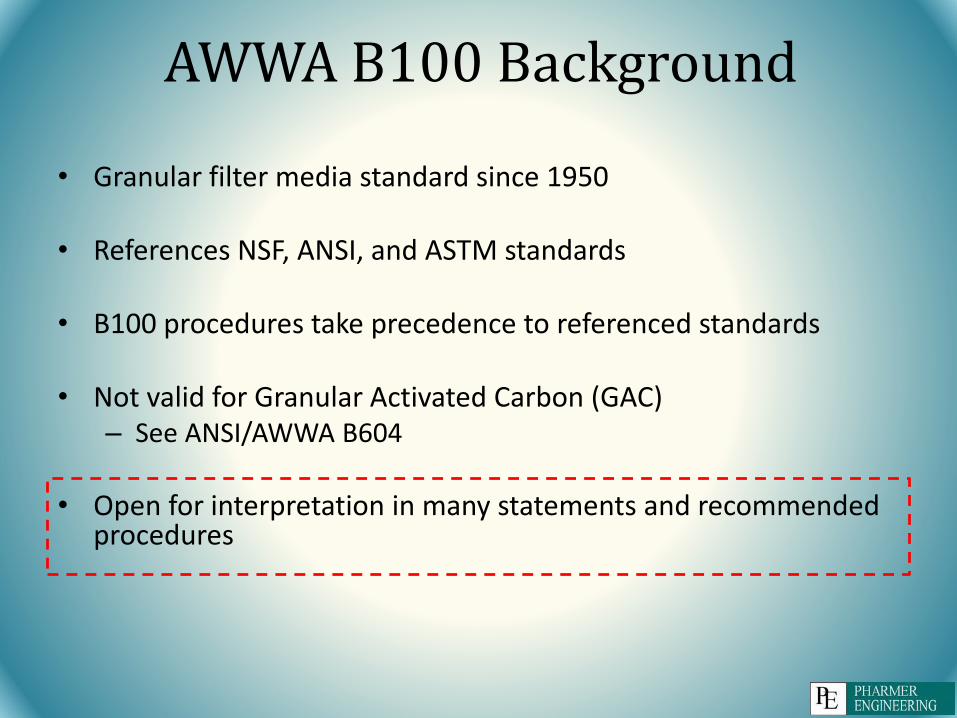
AWWA B100 Background
• Granular filter media standard since 1950
• References NSF, ANSI, and ASTM standards
• B100 procedures take precedence to referenced standards
• Not valid for Granular Activated Carbon (GAC)– See ANSI/AWWA B604
• Open for interpretation in many statements and recommended procedures

Definitions
• Particle Size Distribution – Various size and dimension range description of a filter material determined by standard sieve analysis procedures.
Image courtesy of http://www.cobalt-nickel.comImage courtesy of http://www.analizator.su/

Definitions• Sieve Analysis – The method by which a dry aggregate of known
mass is separated through a series of sieves of progressively smaller openings for determination of particle size distribution.
– In accordance with ASTM C136, as modified and supplemented by AWWA B100.
• Sieve Calibration – A process of verifying the sieve mesh cloth is within allowable tolerances of nominal sizing, either by manufacturer certification or using standard reference material.
– In accordance with ASTM E11, as modified and supplemented by AWWA B100
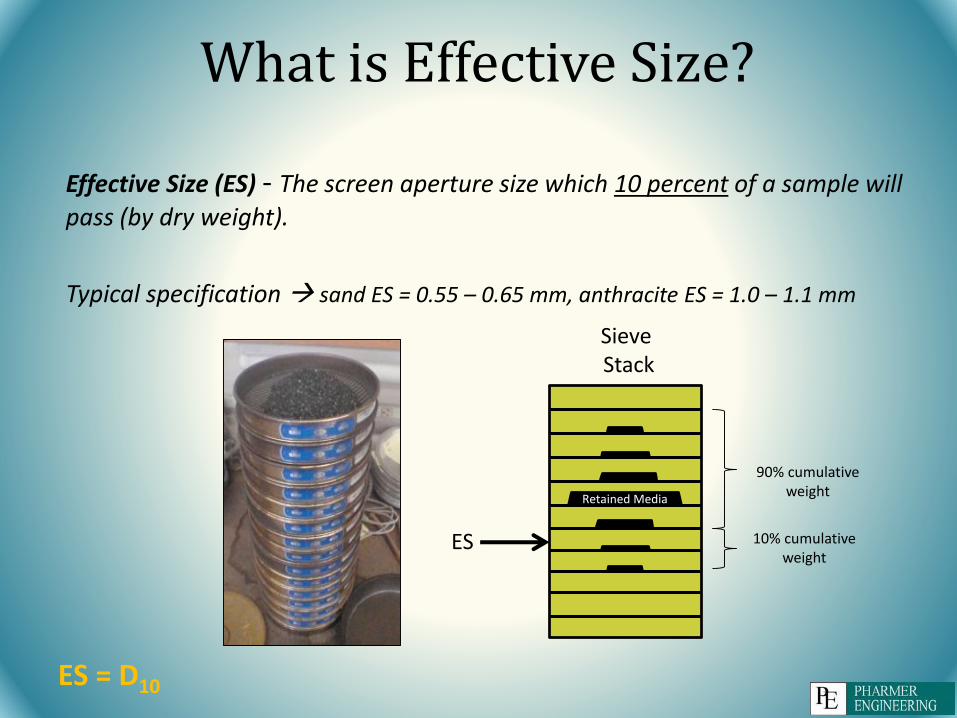
What is Effective Size?
Effective Size (ES) - The screen aperture size which 10 percent of a sample will
pass (by dry weight).
Typical specification sand ES = 0.55 – 0.65 mm, anthracite ES = 1.0 – 1.1 mm
Sieve Stack
Retained Media
90% cumulative weight
10% cumulative weight
ES
ES = D10
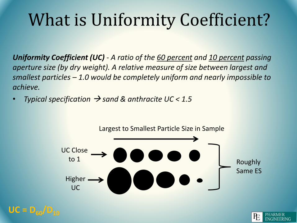
What is Uniformity Coefficient?
Uniformity Coefficient (UC) - A ratio of the 60 percent and 10 percent passing aperture size (by dry weight). A relative measure of size between largest and smallest particles – 1.0 would be completely uniform and nearly impossible to achieve.
• Typical specification sand & anthracite UC < 1.5
UC = D60/D10
Higher UC
Largest to Smallest Particle Size in Sample
UC Close to 1 Roughly
Same ES
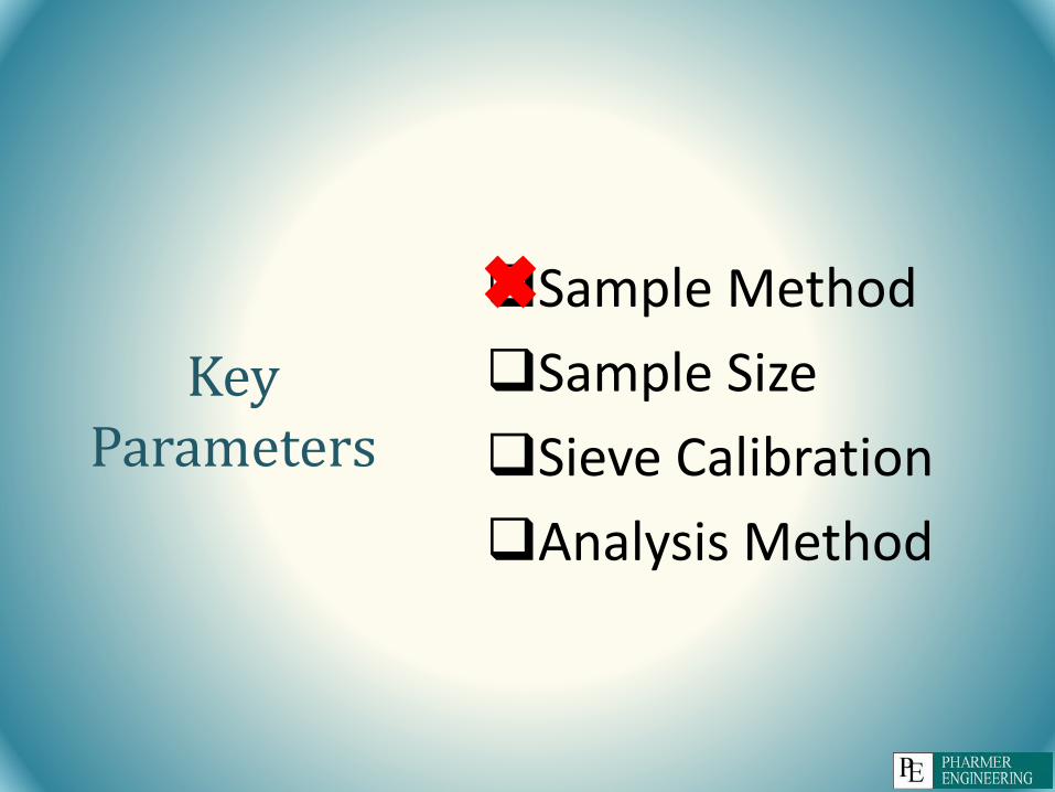
Key Parameters
Sample Method
Sample Size
Sieve Calibration
Analysis Method
Sample Method
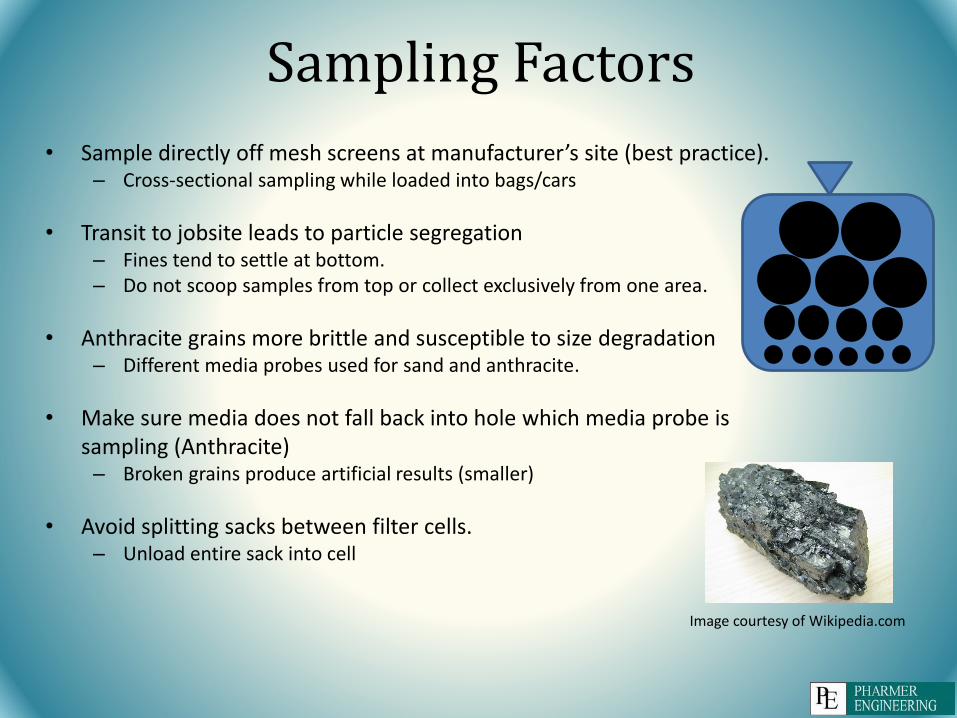
Sampling Factors
• Sample directly off mesh screens at manufacturer’s site (best practice).– Cross-sectional sampling while loaded into bags/cars
• Transit to jobsite leads to particle segregation– Fines tend to settle at bottom.– Do not scoop samples from top or collect exclusively from one area.
• Anthracite grains more brittle and susceptible to size degradation– Different media probes used for sand and anthracite.
• Make sure media does not fall back into hole which media probe is sampling (Anthracite)– Broken grains produce artificial results (smaller)
• Avoid splitting sacks between filter cells.– Unload entire sack into cell
Image courtesy of Wikipedia.com
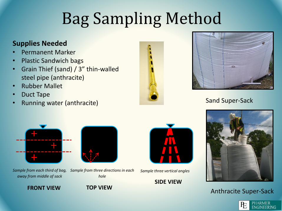
Bag Sampling Method
SIDE VIEW
Sample three vertical angles
Anthracite Super-Sack
Sand Super-Sack
TOP VIEW
Sample from three directions in each
hole
FRONT VIEW
Sample from each third of bag,
away from middle of sack
Supplies Needed• Permanent Marker• Plastic Sandwich bags• Grain Thief (sand) / 3” thin-walled
steel pipe (anthracite)• Rubber Mallet• Duct Tape• Running water (anthracite)

Filter Sampling Method
Supplies Needed• 4’ x 4’ Plywood• Golf Tube or thin PVC – 1.5” D • Sand paper – rough up inside of tube• Individual plastic sandwich bags• Permanent marker
Procedure• Mark each bag in 6” increments, starting at 0”- 6”• Mark the tube in 6” increments (use Whiteout)• Place plywood in filter as sampling base• Use tube to sample first 6” (lightly twist and push down)• Place sample in bag, continue to media interface• Sample from 3 locations (combine like-depth samples) from
3 areas within the filter
1
2
3
Key Parameters
Sample Method
Sample Size
Sieve Calibration
Analysis Method
Sample Size
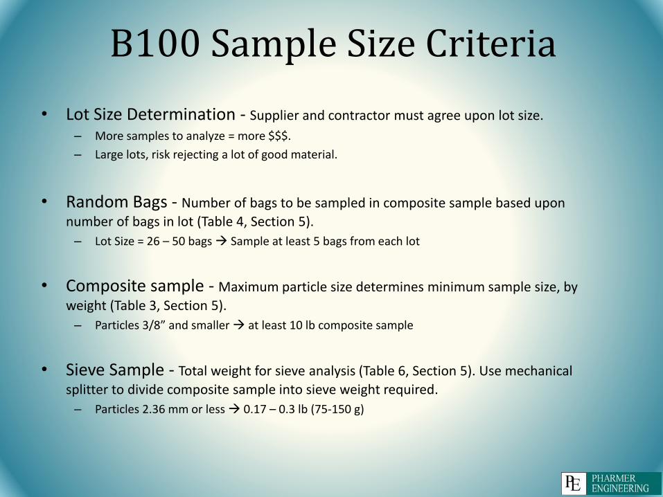
B100 Sample Size Criteria
• Lot Size Determination - Supplier and contractor must agree upon lot size.
– More samples to analyze = more $$$.
– Large lots, risk rejecting a lot of good material.
• Random Bags - Number of bags to be sampled in composite sample based upon
number of bags in lot (Table 4, Section 5).
– Lot Size = 26 – 50 bags Sample at least 5 bags from each lot
• Composite sample - Maximum particle size determines minimum sample size, by
weight (Table 3, Section 5).
– Particles 3/8” and smaller at least 10 lb composite sample
• Sieve Sample - Total weight for sieve analysis (Table 6, Section 5). Use mechanical
splitter to divide composite sample into sieve weight required.
– Particles 2.36 mm or less 0.17 – 0.3 lb (75-150 g)

Sample Size
COMPOSITE SAMPLE
~10 lbs75-150g
LOTRANDOM
SACKS
SPLIT SAMPLE
SIEVE ANALYSIS
Key Parameters
Sample Method
Sample Size
Sieve Calibration
Analysis Method

Sieve Calibration
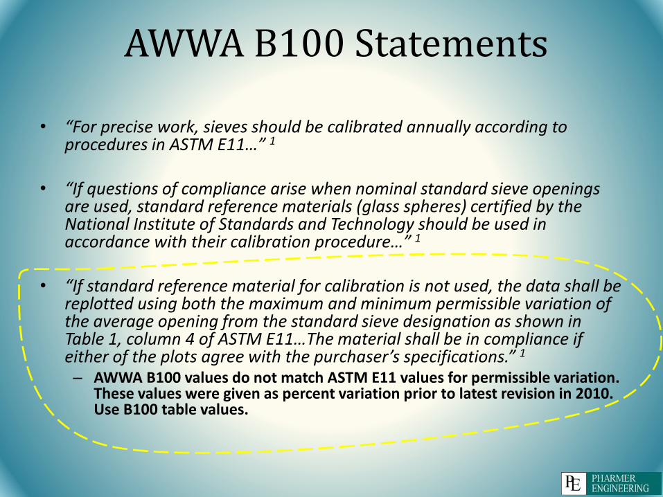
AWWA B100 Statements
• “For precise work, sieves should be calibrated annually according to procedures in ASTM E11…” 1
• “If questions of compliance arise when nominal standard sieve openings are used, standard reference materials (glass spheres) certified by the National Institute of Standards and Technology should be used in accordance with their calibration procedure…” 1
• “If standard reference material for calibration is not used, the data shall be replotted using both the maximum and minimum permissible variation of the average opening from the standard sieve designation as shown in Table 1, column 4 of ASTM E11…The material shall be in compliance if either of the plots agree with the purchaser’s specifications.” 1
– AWWA B100 values do not match ASTM E11 values for permissible variation. These values were given as percent variation prior to latest revision in 2010. Use B100 table values.

Calibration Methods
• Glass spheres - Standard reference material provided by National Institute of Standards and Technology (NIST).– Accuracy ± 1 μm
• Optically Measure – Independently measure or have a certified lab measure.
• Master Calibrated Sieve Stack – Run analysis and check against.
• Certified Calibrated Reference Sample – Run analysis and check against.
• Purchase new certified sieves– Test Sieve Grades 4
• Compliance (66%) – manufactured and inspected to be in compliance with Specification E11, standard test sieve.
• Inspection (99%) – average aperture size, certificate requires inspection data.• Calibration (99.73%) – number of aperture and wire diameters measured,
average aperture size, standard deviation and average wire diameter, certificate requires inspection data.
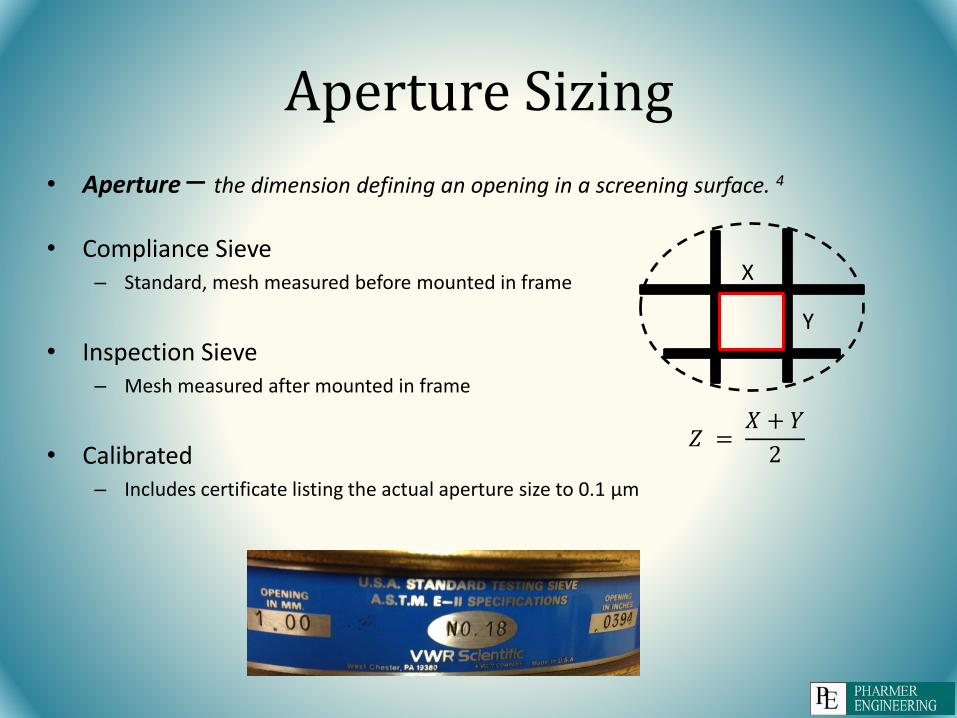
Aperture Sizing
• Aperture – the dimension defining an opening in a screening surface. 4
• Compliance Sieve– Standard, mesh measured before mounted in frame
• Inspection Sieve– Mesh measured after mounted in frame
• Calibrated– Includes certificate listing the actual aperture size to 0.1 μm
𝑍 =𝑋 + 𝑌
2
X
Y
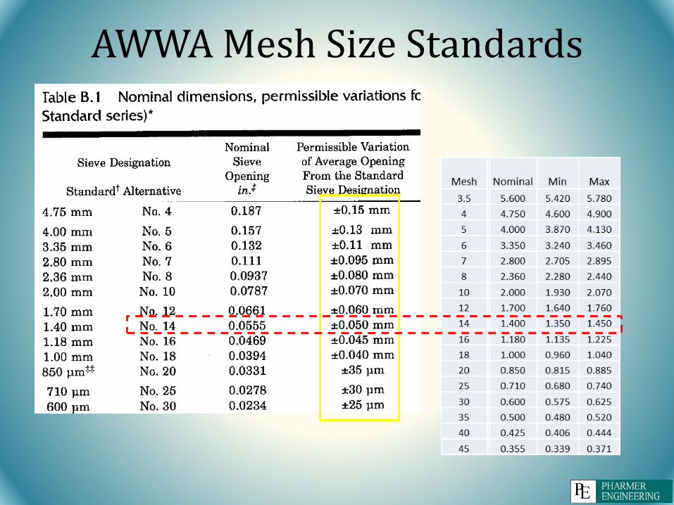
AWWA Mesh Size Standards

Nominal – Minimum – Maximum Variation
__Nominal ES = 1.10Minimum ES = 1.066Maximum ES = 1.153
__Nominal UC = 1.314Minimum UC = 1.319Maximum UC = 1.310
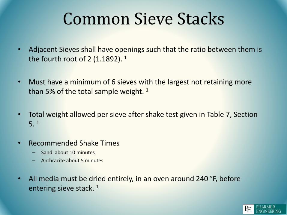
Common Sieve Stacks
• Adjacent Sieves shall have openings such that the ratio between them is the fourth root of 2 (1.1892). 1
• Must have a minimum of 6 sieves with the largest not retaining more than 5% of the total sample weight. 1
• Total weight allowed per sieve after shake test given in Table 7, Section 5. 1
• Recommended Shake Times– Sand about 10 minutes
– Anthracite about 5 minutes
• All media must be dried entirely, in an oven around 240 °F, before entering sieve stack. 1

Key Parameters
Sample Method
Sample Size
Sieve Calibration
Analysis Method
Analysis Method

AWWA Standards
• B100-09 Standards (Latest Revision – 1/09)
– Sieve data plotted on log-probability, graph paper, or comparable computer programs. 1
– No calibration, then replot using maximum and minimum permissible variation of the average opening from the nominal sieve dimension. 1
– A smooth curve is to be drawn through plotted points. 1

Standard Particle Distribution Curve
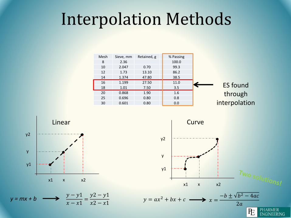
Interpolation Methods
Mesh Sieve, mm Retained, g % Passing
8 2.36 100.0
10 2.047 0.70 99.3
12 1.73 13.10 86.2
14 1.374 47.80 38.5
16 1.199 27.50 11.0
18 1.01 7.50 3.5
20 0.868 1.90 1.6
25 0.696 0.80 0.8
30 0.601 0.80 0.0
ES found through
interpolation
𝑦 = 𝑎𝑥2 + 𝑏𝑥 + 𝑐
x1 x2
y2
y1
y
x
Linear
x1 x2
y2
y1
y
x
Curve
𝑦 − 𝑦1
𝑥 − 𝑥1=𝑦2 − 𝑦1
𝑥2 − 𝑥1y = mx + b 𝑥 =
−𝑏 ± 𝑏2 − 4𝑎𝑐
2𝑎
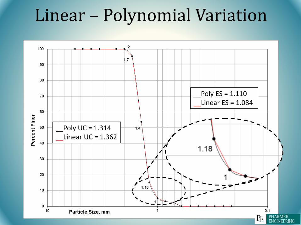
Linear – Polynomial Variation
__Poly ES = 1.110__Linear ES = 1.084
__Poly UC = 1.314__Linear UC = 1.362
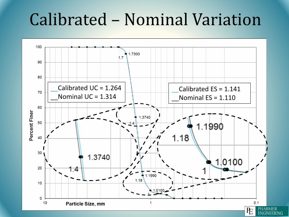
Calibrated – Nominal Variation
__Calibrated ES = 1.141__Nominal ES = 1.110
__Calibrated UC = 1.264__Nominal UC = 1.314
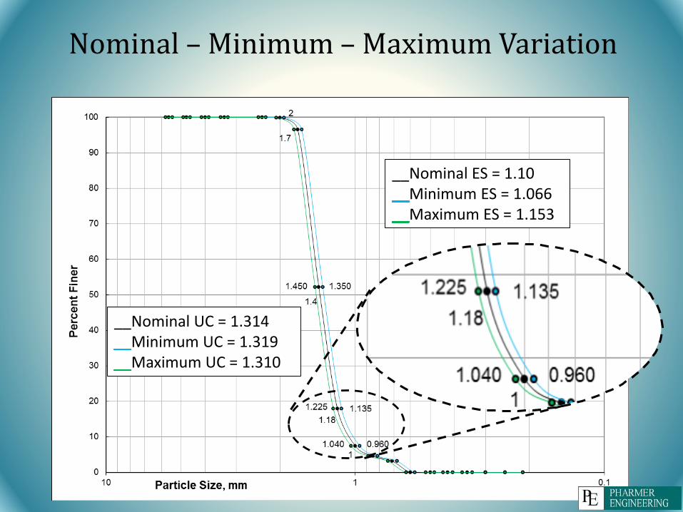
Nominal – Minimum – Maximum Variation
__Nominal ES = 1.10Minimum ES = 1.066Maximum ES = 1.153
__Nominal UC = 1.314Minimum UC = 1.319Maximum UC = 1.310
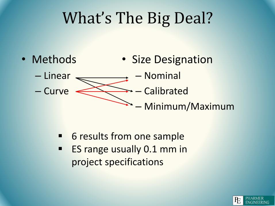
What’s The Big Deal?
• Methods
– Linear
– Curve
• Size Designation
– Nominal
– Calibrated
– Minimum/Maximum
6 results from one sample ES range usually 0.1 mm in
project specifications
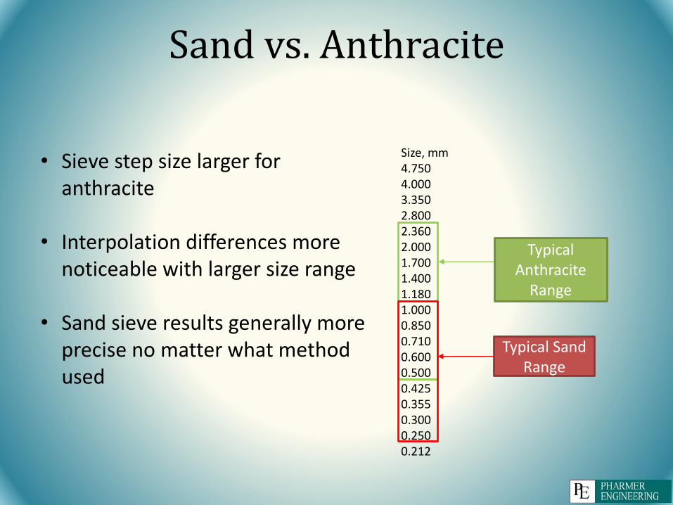
Sand vs. Anthracite
Size, mm4.7504.0003.3502.8002.3602.0001.7001.4001.1801.0000.8500.7100.6000.5000.4250.3550.3000.2500.212
Typical Anthracite
Range
Typical Sand Range
• Sieve step size larger for anthracite
• Interpolation differences more noticeable with larger size range
• Sand sieve results generally more precise no matter what method used
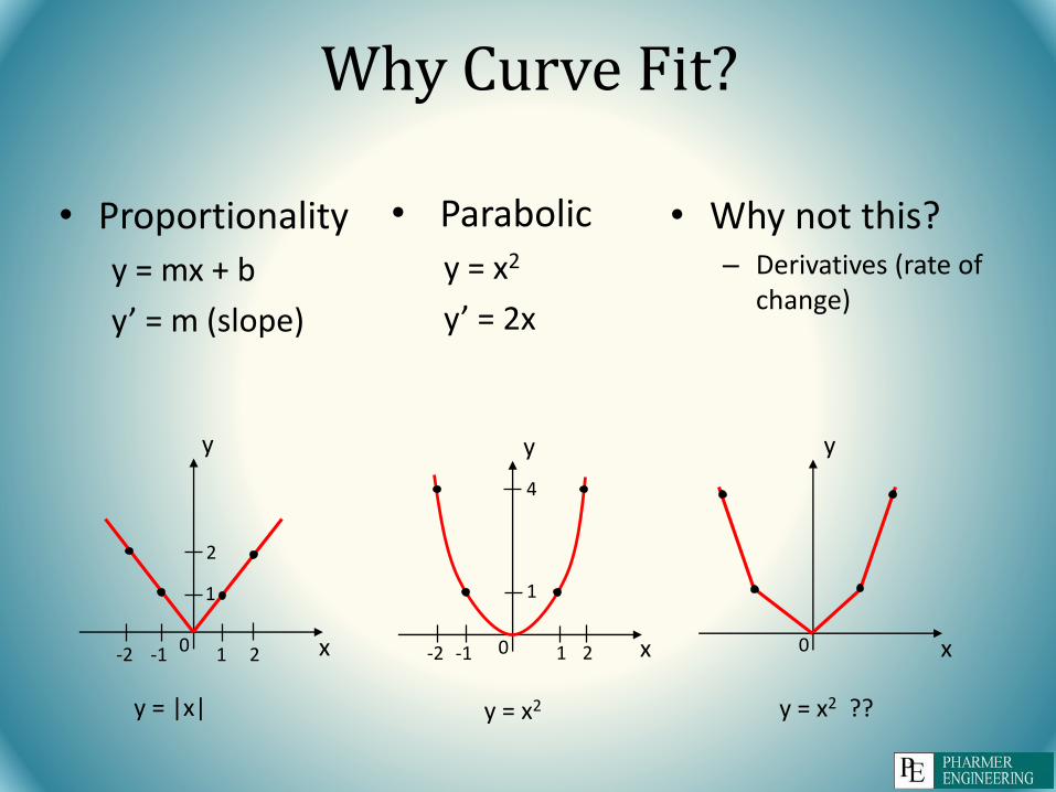
Why Curve Fit?
• Proportionality
y = mx + b
y’ = m (slope)
0 x
y
y = x2 ??
0 x
y
y = |x|
2
-2 -1
1
21 0 x
y
y = x2
21-2 -1
1
4
• Parabolic
y = x2
y’ = 2x
• Why not this?– Derivatives (rate of
change)

Calculus Overview• Curve fitting assumes continuous function for all data points (percent passing)
in interval (sieve size designations), assuming infinite number of sieve sizes in stack to create a smaller step-size, producing a smooth curve.
• Limited data points means interpolating to project results, assuming data points do not fall exactly on known values.
Curve characteristics between data points:
• First Derivative TestIncreasing Decreasingy’ < 0 y’ > 0
Local maximum/minimumy’ = 0
• Second Derivative TestConcave up Concave downy’’ > 0 y’’ < 0
x = (-∞,0) x = (0, ∞)
y = x2 + +
y’ = 2x - +
y’’ = 2 + +
0 x
y
21-2 -1
1
4
Tangent lines (slope)
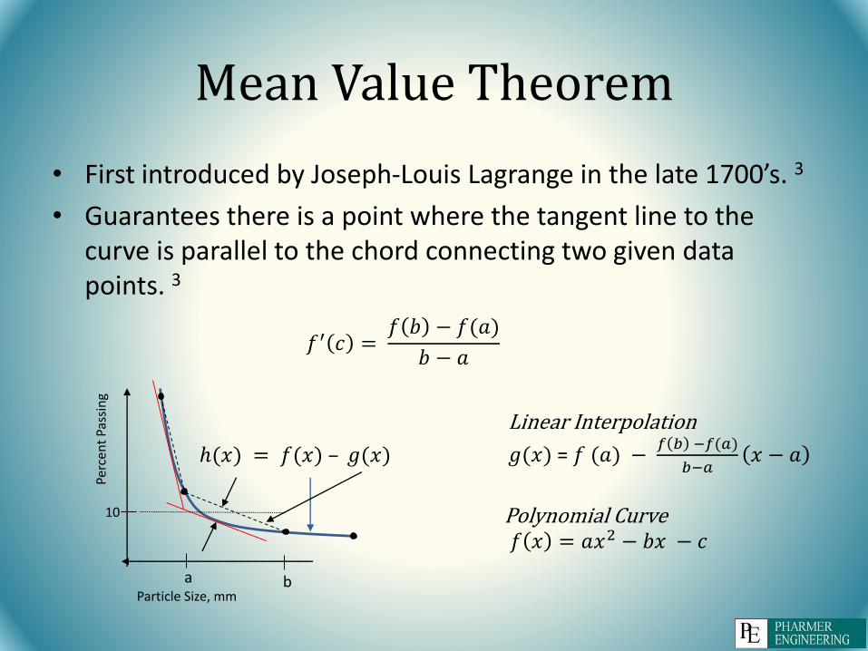
Mean Value Theorem
• First introduced by Joseph-Louis Lagrange in the late 1700’s. 3
• Guarantees there is a point where the tangent line to the curve is parallel to the chord connecting two given data points. 3
Perc
ent
Pass
ing
Particle Size, mm
ℎ(𝑥) = 𝑓(𝑥) – 𝑔(𝑥)
Linear Interpolation
𝑔(𝑥) = 𝑓 (𝑎) −𝑓 𝑏 −𝑓(𝑎)
𝑏−𝑎𝑥 − 𝑎
Polynomial Curve𝑓 𝑥 = 𝑎𝑥2 − 𝑏𝑥 − 𝑐
10
𝑓′ 𝑐 =𝑓 𝑏 − 𝑓(𝑎)
𝑏 − 𝑎
a b
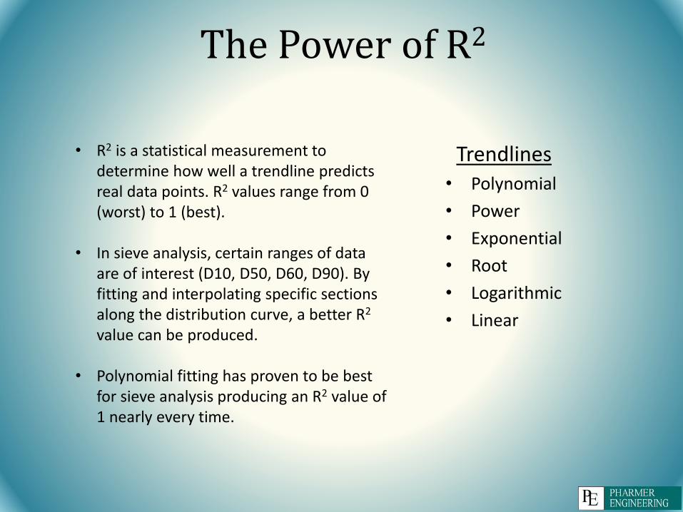
The Power of R2
Trendlines • Polynomial
• Power
• Exponential
• Root
• Logarithmic
• Linear
• R2 is a statistical measurement to determine how well a trendline predicts real data points. R2 values range from 0 (worst) to 1 (best).
• In sieve analysis, certain ranges of data are of interest (D10, D50, D60, D90). By fitting and interpolating specific sections along the distribution curve, a better R2
value can be produced.
• Polynomial fitting has proven to be best for sieve analysis producing an R2 value of 1 nearly every time.

Normal Distribution Curve
__Low UC__Medium UC__High UC
Particle Size
Perc
ent
Ret
ain
ed
+1σ-1σ-2σ +2σ
Mean
μ

High UC – Nominal vs Calibrated
__Nominal ES = 0.999__Calibrated ES = 1.009
__Nominal UC = 1.526__Calibrated UC = 1.510
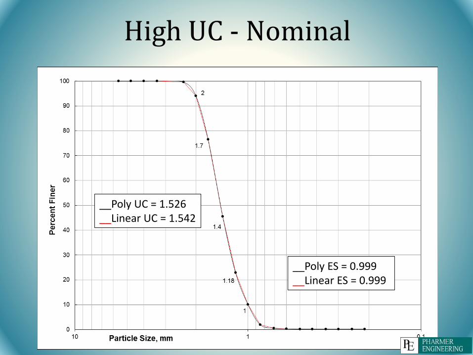
High UC - Nominal
__Poly ES = 0.999__Linear ES = 0.999
__Poly UC = 1.526__Linear UC = 1.542
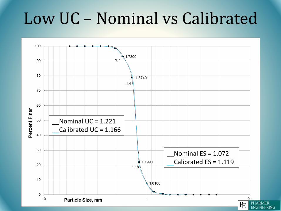
Low UC – Nominal vs Calibrated
__Nominal ES = 1.072__Calibrated ES = 1.119
__Nominal UC = 1.221__Calibrated UC = 1.166

__Poly ES = 1.072__Linear ES = 1.028
__Poly UC = 1.221__Linear UC = 1.291
Low UC - Nominal
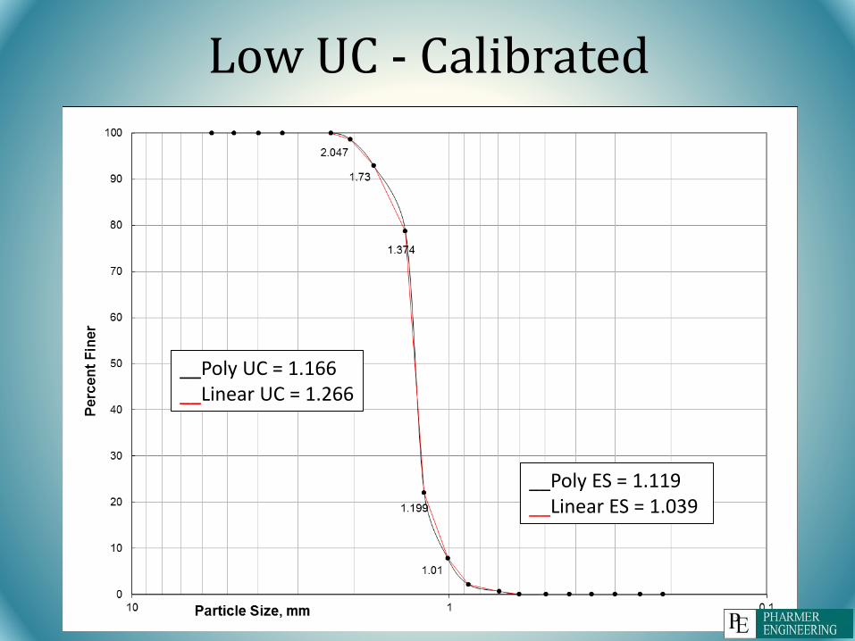
Low UC - Calibrated
__Poly ES = 1.119__Linear ES = 1.039
__Poly UC = 1.166__Linear UC = 1.266
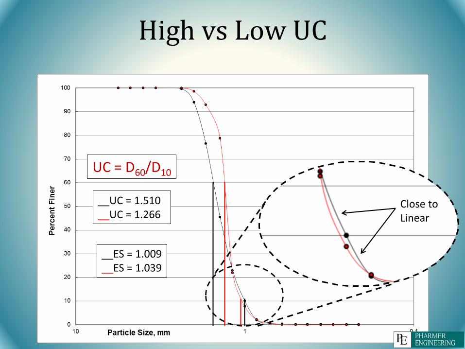
High vs Low UC
__ES = 1.009__ES = 1.039
__UC = 1.510__UC = 1.266
UC = D60/D10
Close to Linear
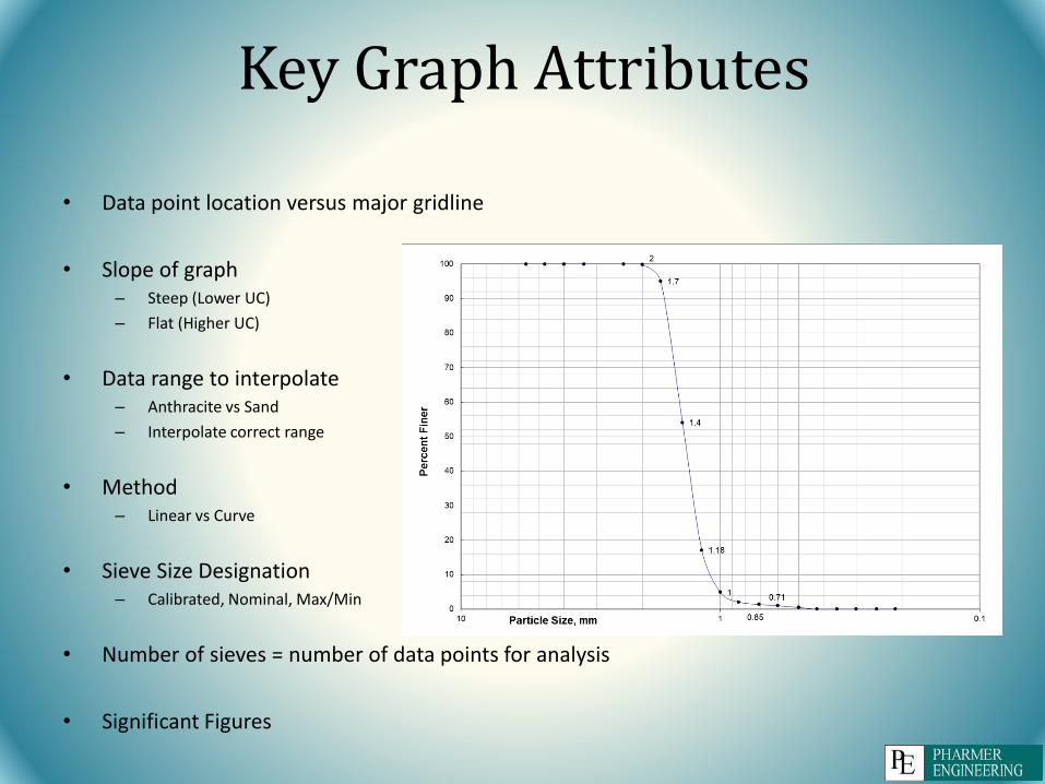
Key Graph Attributes
• Data point location versus major gridline
• Slope of graph – Steep (Lower UC)
– Flat (Higher UC)
• Data range to interpolate– Anthracite vs Sand
– Interpolate correct range
• Method– Linear vs Curve
• Sieve Size Designation– Calibrated, Nominal, Max/Min
• Number of sieves = number of data points for analysis
• Significant Figures

Key Parameters
Sample Method
Sample Size
Sieve Calibration
Analysis Method
Conclusions
• Lower UC material will have major fluctuations between interpolation and calibration methods.
• Methods less important for higher UC material.
• Variance between methods not as noticeable with higher UC samples.
• Sampling methods can vary results.
• Sample size is important to identify and can lead to varied results.
• Equipment calibration can lead to varied results.
• Different analyzing methods can produce varied results.

What does it all mean?
• Tighten quality assurance and enhance performance of filter.
• Increase communication and trust between customer, engineer, contractor, and supplier.
• Saving money and time for all involved with project.

Who Benefits?
• Customer– Receive verified product
– Future maintenance
– Less impact on schedule
• Engineer– Provide more concise
specifications that protect everyone
– Less impact on schedule
• Contractor– Upfront instructions on sampling
methods
– Less impact on schedule
– Avoid multiple interpretations of ambiguous testing criteria
• Supplier– Product is fairly and consistently
tested
– More comfortable to bid job
– Less impact on schedule

Recommendations
• Consistent method for all parties involved with sieve analysis on project– Sampling Techniques
– Sample Sizing
– Sieve Sizing or Calibration
– Analysis Interpolation Method
• Implement maintenance program that contains proper sampling and analysis techniques
• Ask for calibration certificates and analysis methods from lab
References
1AWWA Standard for Granular Filter Material, ANSI/AWWA B100-09, American Waterworks Association, 2009.
2“AWI Standard for Filter Media Sieve Analysis Procedures,” Anthratech U.S. (AWI), 2012.
3Hass, J., Weir, M.D., Thomas, Jr., G.B. (2007). University Calculus: Part One Single Variable. Boston, MA: Pearson Education, Inc.
4ASTM Standard E11, 2009, “Standard Specification for Woven Wire Test Sieve Cloth and Test Sieves,” ASTM International, West Conshohocken, PA, 2009, DOI: 10.1520/E0011-09E01, www.astm.org.

Questions?


![C [AWWA D103 Section 15.1.3] 1.0 [AWWAD103 Section 15.1.1] Il [AWWA 0103 Section 14.2] 1.25 [AWWAD103 Table 2] D [AWWA D103 Table 3] AWWA D103-09; 2013 CBC; ASCE 7 …](https://static.documents.pub/doc/80x56/61284093c2a0803ae83152c0/c-awwa-d103-section-1513-10-awwad103-section-1511-il-awwa-0103-section.jpg)


