80
Beyond the flow decomposition barrier Authors: A. V. Goldberg and Satish Rao (1997) Presented by Yana Branzburg Advanced Algorithms Seminar Instructed by Prof. Haim Kaplan
| Date post: | 21-Dec-2015 |
| Category: |
Documents |
| View: | 213 times |
| Download: | 0 times |

Beyond the flow decomposition barrier
Authors: A. V. Goldberg and Satish Rao (1997)
Presented by Yana BranzburgAdvanced Algorithms Seminar
Instructed by Prof. Haim KaplanTel Aviv University, June 2007

3
Introduction
Maximum flow problem Use the concept of distance Distance is defined by arc length Methods so far use unit length
function Goldberg&Rao use adaptive binary
length function: length threshold is set relative to an estimate of residual flow

4
Ω(mn) barrier Ω(mn) - a natural barrier for maximum
flow algorithms that output explicit flow decomposition (the
total path length is Θ(mn) in the worst case) that augment flow one path at the time, for
each augmenting path, one arc at the time Although the barrier does not apply to
algorithms that use preflows or data structures like dynamic trees, no one beats it

5
Ω(mn) barrier (cont.)

6
Beyond the Ω(mn) barrier Dinic’s algorithm for unit-capacity
networks
Goldberg-Rao algorithm for general networks
)},(min{ 3/22/1 mnmO
)log)log(},(min{2
3/22/1 Um
nmnmO

7
Background flow network:
G = (V, E) source s, sink t capacity function u: E {1, …, U}
flow function f: E {1, …, U} f(a) ≤ u(a) conservation constraint
flow value is
0),(),(},,{),( ),(
wv vuvufwvftsVj
),(
),(tv
tvff

8
Background (cont.) residual capacity uf (v,w) = u(v,w) –
f(v,w) + f(w,v) Arc (v,w) is a residual arc if uf (v,w) > 0 residual flow is the difference between
optimal flow f* and current flow f In blocking flow every directed path s-t
contains an arc with residual capacity 0 Without loss of generality assume:
G has no parallel arcs if arc (v,w) is in G, but (w,v) is not, add (w,v)
to G, define u(w,v)=0 either f(v,w) = 0 or f(w,v) = 0

Dinic’s algorithm for unit-capacity networks

10
Dinic’s algorithm for unit capacity networks A unit capacity network is one in which
all arc have unit capacities Algorithm of two phases:
Find augmenting paths, until distance between s and t is
Augment the found flow to an optimal flow
}2,min{ 3/22/1 nm

11
Dinic’s algorithm for unit capacity networks (cont.) Algorithm Dinic
while ds ≤ α (ds stands for length of the shortest path from s to t)
Find blocking flow in admissible network Compute residual network
while there is an s-t path in the residual network
Find an s-t path P Augment one unit of flow along P Compute residual network
12
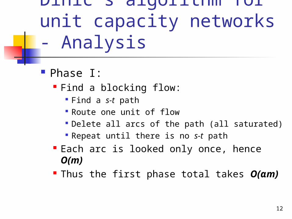
Dinic’s algorithm for unit capacity networks - Analysis
Phase I: Find a blocking flow:
Find a s-t path Route one unit of flow Delete all arcs of the path (all saturated) Repeat until there is no s-t path
Each arc is looked only once, hence O(m)
Thus the first phase total takes O(αm)

13
Dinic’s algorithm for unit capacity networks – Analysis (cont.)
Phase II: Blocking flow increases the distance
between s and t by at least one Let the vertices be partitioned into
levels
Thus, at the end of phase I, there are at least α levels
svk dkkdVvV ,...,0,|

14
Dinic’s algorithm for unit capacity networks – Analysis (cont.)
Lemma 1: At the end of phase I, the maximum flow in the residual network is at most α
Proof. Case 1: α = m½
At least m½ levels and m arcs there is a pair of adjacent levels Vk and Vk+1 which have at most m½ arcs between them
The cut has capacity at most m½ maximum residual flow is m½
),(0 1 k
i
d
ki iis VV

15
Dinic’s algorithm for unit capacity networks – Analysis (cont.)
Proof. Case 2: α = 2n ⅔
There exists a pair of adjacent levels Vk and Vk+1 , each of which has at most n ⅓ nodes
Assume the contrary: at least half levels must contain more than n ⅓ nodes
Then the total number of nodes more than α/2*n ⅓ ≥ n, which is a contradiction
Thus the cut has capacity at most n ⅔ ≤ α
),(0 1 k
i
d
ki iis VV

16
Dinic’s algorithm for unit capacity networks – Analysis (cont.)
Each iteration of phase II routes one unit of additional flow
Since after phase I the maximum flow in the residual network ≤ α, the maximum number of iterations in phase II is bounded by α
One iteration of phase II is O(m) Thus, the second phase takes total O(αm) Hence, Dinic’s algorithm for unit capacity
networks solves the maximum flow problem in time)},(min{ 3/22/1 mnmO

Goldberg-Rao algorithm

18
Length Functions length function ℓ : E R+
distance labeling d : V R+ with respect to a length function ℓ if:
d(t) = 0 for every (v,w) in E : d(v) ≤ d(w) + ℓ(v,w)
admissible arc (v,w) is a residual arc where d(v) > d(w) or d(v) = d(w) and ℓ(v,w) = 0
In case of binary length function, admissible arc satisfies d(v) = d(w) + ℓ(v,w)
distance function dℓ(v) : distance from v to t under ℓ
dℓ(v) is a distance labeling

19
Length Functions (cont.)
Claim 2: dℓ is the biggest distance labeling Proof (assume the contrary):
d(v) >dℓ(v) for some v w is the last node on a shortest v-t path Γ
that satisfies d(w) >dℓ(w) x follows w (w ≠t, hence x exists) dℓ(w) < d(w) ≤ ℓ(w,x) +d(x) ≤ ℓ(w,x) +dℓ(x) v-w concatenated with w-t is shorter than Γ Contradiction to selection of Γ

20
Volume of Network A residual arc a has
“width” uf(a) length ℓ(a) volume volf,ℓ(a) = uf(a) ℓ(a)
network volume Volf,ℓ = Σauf(a) ℓ(a) The residual flow value is upper bounded
by Volf,ℓ ∕dℓ(s) (since any path from s to t has length at least dℓ(s) > 0)
To get a tighter bound, keep Volf,ℓ small by choosing a binary length function that is zero for large residual capacity arcs

21
Binary Blocking Flow Algorithm - Idea Ensure the algorithms terminates after
not too many augmentations by showing that every iteration increases dℓ(s) - but we have zero arcs?! Contract strongly connected components
(nodes) formed by zero-length arcs Bound the augmenting flow in a node by Δ to
be able to reroute the flow in a restored node
Possible not to find a blocking flow can not guarantee increase of dℓ(s)
Choose Δ that insures small number of non-blocking augmentations

23
Stopping Condition of the Algorithm
Define F - an upper bound on the residual flow value
Update F every time our estimate improves
Stop when F < 1 (integral capacities)
Initial estimate is F = Σ(s,w)u(s,w) ≤ nU

24
The Skeleton of Goldberg-Rao algorithm while F ≥ 1 do
Compute Δ while the residual capacity > F /2
Compute length function ℓ, distance function dℓ
Find admissible graph A(f, ℓ, dℓ) Contract strongly connected components of A Find a flow of value Δ or a blocking flow Augment the current flow, extend it to original
graph and recompute the residual graph Update F
upd
ate
st
ep
phase

25
Estimate a residual capacity A residual capacity uf(S,T) of an s-t cut
can serve as an upper bound canonical cut (Sk ,Tk) :
(Sk ,Tk) is an s-t cut Initially (S,T) =({s },V \{s }) is the
current cut Find a canonical cut with the smallest
residual capacity When the capacity of the found cut ≤
F /2, update F to this capacity value
)(,...,1,\,)(| sdkSVTkvdVvS lkklk

26
Estimate a residual capacity (cont.) Claim 3: The minimum capacity
canonical cut can be found in O(m) time Proof:
Every arc may cross at most one canonical cut (its length at most 1)
For k =1,…,dℓ(s), initialize uf(Sk,Tk) =0 For every arc (v,w) : if dℓ(v) > dℓ(w), increase
uf(Sk,Tk) by uf(v,w), k = dℓ(v) Find minimum among all uf(Sk,Tk) Denote the minimum capacity canonical cut
),( TS

27
Binary length function
A first estimate of a length function:
* this length function will have to be modified for reasons that will come up during time analysis
Given ℓ, next we show how to handle the contraction of zero arcs
otherwise
auifal
f
,1
2)(,0)(

28
Extending the flow inside contracted components Claim 4: Given a flow of value at
most Δ, we can correct it to a flow of the same value in the original graph in O(m) time
Proof (for one component): Choose an arbitrary vertex as a root Form an in-tree and an out-tree
in-tree: a rooted tree with a path from each node to the root
out-tree: a rooted tree with a path from the root to each node

29
Extending the flow inside contracted components (cont.) Proof (cont.):
For each vertex compute its flow balance: sum of flow entering minus sum of flow leaving the vertex
Route the positive balances to the root using the in-tree
Route the resulting flow excess from the room to negative balances via out-tree
At most Δ flow is routed to and from the root using one arc, which residual capacity is at least 2Δ

30
Example:
0.5Δ
R
out treein tree
Extending the flow inside contracted components (cont.)
0.5Δ
0.75Δ
0.25Δ
+0.5Δ
+0.5Δ
-0.75 Δ
-0.25 Δ
0.5Δ Δ
Δ
Δ
Δ
+Δ +Δ
+0.25Δ

31
Time bounds Reminder: choice of Δ must insure small
number of non blocking augmentations Denote Let Thus, number of non blocking
augmentations of value Δ is at most α in each phase
How many blocking augmentations per phase there are? Need to show that O(α)
F},min{ 3/22/1 nm

32
Bound of number of blocking augmentations Lemma 5: For a 0-1 length function on the
residual graph:
where M is the maximum residual capacity of a length one arc
Proof: Every arc crosses at most one of the canonical cuts,
for such an arc, ℓ(a) =1 Total capacity of length one arcs ≤ mM, there are
dℓ(s) canonical cuts Thus, minimum capacity canonical cut ≤ mM / dℓ(s)
Msd
mTSu
lf )(
),(

33
Bound of number of blocking augmentations (cont.)
For dense graphs, the following Lemma gives better bounds
Lemma 6: For a 0-1 length function on the residual graph:
Proof: Let Since , there are at most dℓ(s)/2 values of k
where |Vk | > 2n /dℓ(s) Thus, at least values of k have |Vk | ≤ 2n /dℓ(s) By the pigeonhole principle, there is j such that
|Vj | ≤ 2n /dℓ(s) and |Vj+1 | ≤ 2n /dℓ(s) Since all arcs from Vj+1 to Vj have length 1, Lemma 6
holds
)(,...,0,)(| sdkkvdVvV llk
Msd
nTSu
lf
2
)(
2),(
nVsd
k kl
)(
0
12/)( sdl

34
Bound of number of blocking augmentations (cont.) Lemma 7: In every iteration of a
blocking flow, dℓ(s) increases by at least 1 (prove later)
Lemma 8: There are at most O(α) blocking flow augmentations in a phase
Proof: Case 1: α = m½
Using Lemma 7: after 4m½ blocking flow update steps dℓ(s) ≥ 4m½
M ≤ 2Δ. Thus, together with Lemma 5:24
22)()(
),(F
m
F
m
m
sd
mM
sd
mTSu
llf

35
Bound of number of blocking augmentations (cont.) Proof. Case 2: α = n ⅔
Using Lemma 7: after 4n ⅔ blocking flow update steps dℓ(s) ≥ 4n ⅔
M ≤ 2Δ. Thus, together with Lemma 6:
Conclusion: Each phase of the algorithm terminates in O(α) update steps
24
222
)(
2
)(
2),(
3/2
2
3/2
22F
n
F
n
n
sd
nM
sd
nTSu
llf

36
Finding a flow in one update step We use Goldberg&Tarjan algorithm
for computing a blocking flow X in each update step in O(m ּlog(n2/m)) time
If X > Δ, return extra flow to s in O(m) time: Place X – Δ units of excess at t Process vertices in reverse topological
order For current vertex reduce flow on the
incoming arcs to eliminate its excess

37
Time Bounds Summary Theorem 9: The maximum flow problem
can be solved in O(αּmּlog(n2/m)ּlogU) time
Proof: Δ>U : all arcs are length one Each update step finds a blocking flow
and increases dℓ(s) by at least one After α steps dℓ(s) ≥α F ≤αU After O(α) steps F =α Δ ≤αU Δ≤U Total time till Δ =U is O(αּmּlog(n2/m))
F =uf(S,T) ≤ mM /dℓ(s) ≤ mM /α =
αM ≤ αU

38
Time Bounds Summary (cont.)
Proof (cont.): 1≤Δ≤U : Number of phases is
O(logU), since each phase decreases twice
Total time for these phases is O(αּmּlog(n2/m)ּlogU)
When Δ=1, F ≤α, the algorithm ends in O(α) update steps
F

39
Proof of Lemma 7
In every iteration of a blocking flow, dℓ(s) increases by at least 1
Denote: ℓ and dℓ - initial length and distance
functions ℓ’ and dℓ’ - after finding a blocking flow
and recomputing the residual graph f and f’ - the flows before and after
augmentation respectively
Need to prove: dℓ(s) < dℓ’ (s)

40
Proof of Lemma 7 (cont.) Claim 10: dℓ is a distance labeling
with respect to ℓ’ Proof:
By definition: dℓ(v) ≤ dℓ(w) + ℓ(v,w) Need to show: dℓ(v) ≤ dℓ(w) + ℓ’(v,w) If dℓ(v) ≤ dℓ(w) – trivial dℓ(v) >dℓ(w) (w,v) is not admissible
(for admissible arc dℓ(w)=dℓ(v)+ℓ(w,v)) uf’ (v,w) ≤ uf(v,w) ℓ’(v,w) ≥ ℓ(v,w)

41
Proof of Lemma 7 (cont.)
Claim 11: dℓ(s) ≤ dℓ’ (s) Proof:
By Claim 2: for any distance labeling d, d(v) ≤ dℓ(v)
By Claim 10: dℓ is a distance labeling with respect to ℓ’
dℓ(s) ≤ dℓ’ (s)

42
Proof of Lemma 7 (cont.) We need to show dℓ(s) < dℓ’ (s) Let Γ be an s-t path in Gf’
By Claim 10:cost(v,w) =dℓ(w) -dℓ(v) +ℓ’(v,w) ≥0
ℓ’ (Γ) = dℓ(s) –dℓ(v1) +c(s,v1) +
dℓ(v1) –dℓ(v2) +c(v1,v2) +…+
dℓ(vk) –dℓ(t) +c(vk,t) =
dℓ(s) – dℓ(t) +c (Γ) = dℓ(s) +c (Γ)

43
Proof of Lemma 7 (cont.)
dℓ’ (s) = ℓ’ (Γ) = dℓ(s) + c (Γ) Enough to show that along every s-
t path Γ in Gf’ there is an arc (v,w) satisfying c(v,w) > 0

44
Proof of Lemma 7 (cont.)
We routed a blocking flow Γ contains arc (v,w) that is not in A(f, ℓ, dℓ)
dℓ(v) ≤ dℓ(w) either because: (v,w) in Gf (otherwise (v,w) would be in
A(f, ℓ, dℓ)) or (v,w) not in Gf but in Gf’ (means that (w,v)
is in A(f, ℓ, dℓ) dℓ(w) = dℓ(v) + ℓ(v,w) dℓ(w) ≥dℓ(v))
dℓ(v) >dℓ(w):
dℓ(v) ≤ dℓ(w) + ℓ(v,w)< dℓ(v) + ℓ(v,w)
ℓ(v,w) > 0 dℓ(v) = dℓ(w) + ℓ(v,w)

45
Proof of Lemma 7 (cont.) Assume the contrary that
c(v,w) =dℓ(w) -dℓ(v) +ℓ’(v,w) = 0 dℓ(v) ≤dℓ(w) dℓ(w) =dℓ(v) and ℓ’(v,w) =0 Case 1 - (v,w) in Gf :
1=ℓ(v,w) >ℓ’(v,w) =0(w,v) is in A(f, ℓ, dℓ)
Case 2 - (v,w) not in Gf but in Gf’ : (w,v) is in A(f, ℓ, dℓ)
But dℓ(w) =dℓ(v) ℓ (w,v) = 0

46
Bad Example
dℓ(w) =dℓ(v), ℓ(w,v) =0 and ℓ’(v,w) =0 Δ ≤ uf(v,w) < 2Δ uf(w,v) > 2Δ
uf’ (v,w) ≥ uf(v,w) + 2Δ – uf(v,w) ≥ 2Δ ℓ’(v,w) = 0
vw
≥ 2Δ- uf(v,w)

47
Solution to bad example Distort the length function, so that
such bad arcs get length zero ahead
Might become an inner arc in a strongly connected component
The capacity of such arcs must be at least 2Δ in order to be able to route a flow of Δ in flow extension (remember example…)
48
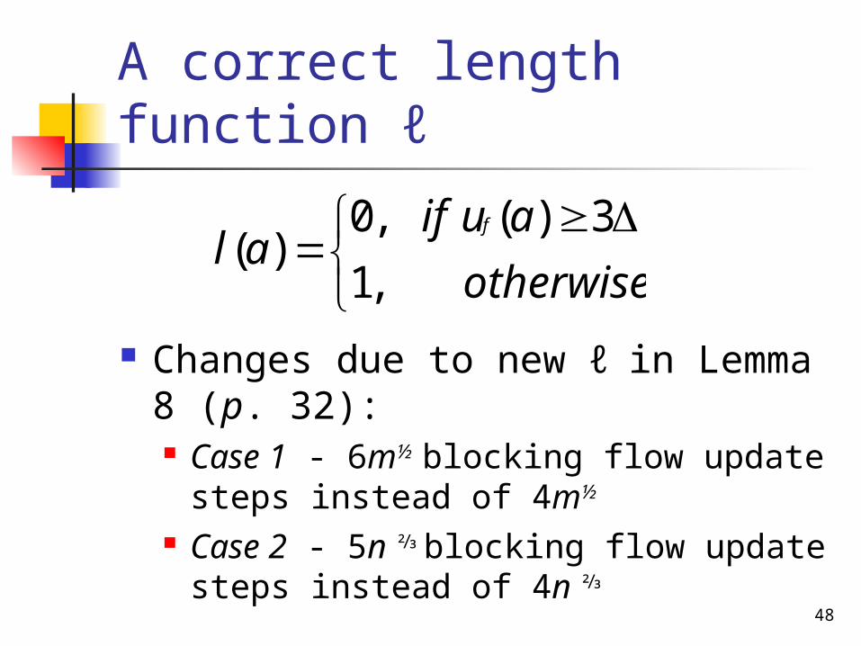
A correct length function ℓ
Changes due to new ℓ in Lemma 8 (p. 32): Case 1 - 6m½ blocking flow update
steps instead of 4m½
Case 2 - 5n ⅔ blocking flow update steps instead of 4n ⅔
otherwise
auifal
f
,1
3)(,0)(

49
Length function ℓ* (v,w) is a special arc if:
2Δ ≤ uf(v,w) < 3Δ d(v) =d(w) uf(w,v) ≥ 3Δ
Define new length function ℓ* that: = zero on special arcs = ℓ on all other arcs
dℓ* = dℓ
The algorithm determines admissible graph A(f, ℓ*, dℓ) instead of A(f, ℓ, dℓ)

50
Proof of Lemma 7 using ℓ* dℓ(w) =dℓ(v), ℓ(w,v) =0 and ℓ’(v,w) =0 ℓ(w,v) =0 uf(w,v) ≥ 3Δ ℓ’(v,w) =0 uf’ (v,w) ≥ 3Δ (w,v) is in A(f, ℓ*, dℓ) pushing a flow
(at most Δ) increased uf’ (v,w) uf(v,w) ≥ 2Δ Either (v,w) is a special arc before
augmentation or uf(v,w) ≥ 3Δ (v,w) is in A(f, ℓ*, dℓ) - contradiction

51
Example
T
12
S
16
13
910
4
14
20
74
while F ≥ 1 do
Compute Δ, ℓ, dℓ
while (S,T) > F /2
Compute ℓ*
Find A(f, ℓ*, dℓ)
Contract SCC of A
Find a flow f*
f’ = f + f*
Extend f* to G
Recompute ℓ,dℓ,Gf’
Update F
n = 6, m = 10 U = 20 F = 29 α = min{m½, n ⅔ } = 4 Δ = F /α = 8

52
Example (cont.)2 1
1
0
12
3
2
16
13
910
4
14
20
74
1Gf :
1
1
1
1
1
11
1
1
F = 29. Δ = 8 2 1
1
0
4/12
3
2
4/16
4/13 4/14
4/20
4/4
1Af :
1
1
1
1
1
while F ≥ 1 do
Compute Δ, ℓ, dℓ
while (S,T) > F /2
Compute ℓ*
Find A(f, ℓ*, dℓ)
Contract SCC of A
Find a flow f*
f’ = f + f*
Extend f* to G
Recompute ℓ,dℓ,Gf’
Update F

53
Example (cont.)1 2 1
2
0
8
3
3
12
9
910
4
10
16
74
1Gf ‘:
1
1
1
1
1
11
1
1
4
44
44
11
1
1
F = 29. Δ = 8(S,T) = 15
while F ≥ 1 do
Compute Δ, ℓ, dℓ
while (S,T) > F /2
Compute ℓ*
Find A(f, ℓ*, dℓ)
Contract SCC of A
Find a flow f*
f’ = f + f*
Extend f* to G
Recompute ℓ,dℓ,Gf’
Update F
54
Example (cont.)
3
2 1
2
0
8/8
3
8/12
0/10
8/161
Af’ :1
1
1
0/7
1
0/4
1
F = 29. Δ = 8
1 2 1
2
0
8
3
3
12
9
910
4
10
16
74
1Gf ‘:
1
1
1
1
1
11
1
1
4
44
44
11
1
1while F ≥ 1 do
Compute Δ, ℓ, dℓ
while (S,T) > F /2
Compute ℓ*
Find A(f, ℓ*, dℓ)
Contract SCC of A
Find a flow f*
f’ = f + f*
Extend f* to G
Recompute ℓ,dℓ,Gf’
Update F
55
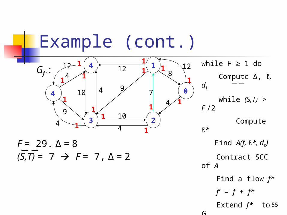
Example (cont.)1 4 1
2
0
12
4
3
4
9
910
4
10
8
74
1Gf ‘:
1
1
1
1
1
11
1
1
12
44
12
11
1
F = 29. Δ = 8(S,T) = 7 F = 7, Δ = 2
while F ≥ 1 do
Compute Δ, ℓ, dℓ
while (S,T) > F /2
Compute ℓ*
Find A(f, ℓ*, dℓ)
Contract SCC of A
Find a flow f*
f’ = f + f*
Extend f* to G
Recompute ℓ,dℓ,Gf’
Update F

56
Example (cont.)
F = 7. Δ = 2
0 0 0
0
0
12
0
0
4
9
910
4
10
8
74
0Gf ‘:
0
0
0
0
0
00
0
1
12
44
12
00
0
while F ≥ 1 do
Compute Δ, ℓ, dℓ
while (S,T) > F /2
Compute ℓ*
Find A(f, ℓ*, dℓ)
Contract SCC of A
Find a flow f*
f’ = f + f*
Extend f* to G
Recompute ℓ,dℓ,Gf’
Update F
0 0 0
0
0
12
0
0
4
2/9
910
4
2/10
2/8
2/7
0Af ‘:
0
0
0
0
0
00
012
44
12
00
0

57
Example (cont.)0 1 0
1
0
12
1
1
4
7
910
4
8
6
54
1Gf ‘:
0
0
0
1
0
01
0
1
12
66
14
00
0
2
1
F = 7. Δ = 2(S,T) = 5
while F ≥ 1 do
Compute Δ, ℓ, dℓ
while (S,T) > F /2
Compute ℓ*
Find A(f, ℓ*, dℓ)
Contract SCC of A
Find a flow f*
f’ = f + f*
Extend f* to G
Recompute ℓ,dℓ,Gf’
Update F

58
while F ≥ 1 do
Compute Δ, ℓ, dℓ
while (S,T) > F /2
Compute ℓ*
Find A(f, ℓ*, dℓ)
Contract SCC of A
Find a flow f*
f’ = f + f*
Extend f* to G
Recompute ℓ,dℓ,Gf’
Update F
Example (cont.)
F = 7. Δ = 260
0 1 0
1
0
12
1
1
4
7
910
4
8
6
54
0Gf ‘:
0
0
0
0
0
01
0
1
12
6
140
2
1
0
0 1 0
1
01
1
4
2/7
10
4
2/8
2/6
2/5
0Af ‘:
0
0
00
1
012
44
12
00
0

59
80
0 1 0
1
0
12
2
1
4
5
910
4
6
4
34
1Gf ‘:
1
0
0
1
0
01
0
1
12
8
160
4
1
Example (cont.)while F ≥ 1 do
Compute Δ, ℓ, dℓ
while (S,T) > F /2
Compute ℓ*
Find A(f, ℓ*, dℓ)
Contract SCC of A
Find a flow f*
f’ = f + f*
Extend f* to G
Recompute ℓ,dℓ,Gf’
Update F
F = 7. Δ = 2(S,T) = 3 F = 3, Δ = 1
0

60
while F ≥ 1 do
Compute Δ, ℓ, dℓ
while (S,T) > F /2
Compute ℓ*
Find A(f, ℓ*, dℓ)
Contract SCC of A
Find a flow f*
f’ = f + f*
Extend f* to G
Recompute ℓ,dℓ,Gf’
Update F
Example (cont.)
F = 3. Δ = 180
0 0 0
0
0
12
0
0
4
5
910
4
6
4
34
0Gf ‘:
0
0
0
0
0
00
0
0
12
8
160
4
0
80
0 0 0
0
0
12
0
0
4
1/5
910
4
1/6
1/4
1/3 4
0Af ‘:
0
0
0
0
0
00
0
0
12
8
160
4
0

61
Example (cont.)while F ≥ 1 do
Compute Δ, ℓ, dℓ
while (S,T) > F /2
Compute ℓ*
Find A(f, ℓ*, dℓ)
Contract SCC of A
Find a flow f*
f’ = f + f*
Extend f* to G
Recompute ℓ,dℓ,Gf’
Update F
F = 3. Δ = 1(S,T) = 2
90
0 1 0
1
0
12
1
1
4
4
910
4
5
3
24
0Gf ‘:
0
0
0
0
0
01
0
0
12
9
170
5
0
0

62
while F ≥ 1 do
Compute Δ, ℓ, dℓ
while (S,T) > F /2
Compute ℓ*
Find A(f, ℓ*, dℓ)
Contract SCC of A
Find a flow f*
f’ = f + f*
Extend f* to G
Recompute ℓ,dℓ,Gf’
Update F
Example (cont.)
F = 3. Δ = 190
0 1 0
1
0
12
1
1
4
4
910
4
5
3
24
0Gf ‘:
0
0
0
0
0
01
0
0
12
9
170
5
0
0
90
0 1 0
1
01
1
4
1/4
10
4
1/5
1/3
1/2
0Af ‘:
0
0
00
1
012
9
170
0

63
while F ≥ 1 do
Compute Δ, ℓ, dℓ
while (S,T) > F /2
Compute ℓ*
Find A(f, ℓ*, dℓ)
Contract SCC of A
Find a flow f*
f’ = f + f*
Extend f* to G
Recompute ℓ,dℓ,Gf’
Update F
Example (cont.)
F = 3. Δ = 1(S,T) = 1 F = 1, Δ = 1
10
0
0 2 1
2
0
12
2
2
4
3
910
4
4
2
14
0Gf ‘:
0
0
0
0
0
01
1
0
12
10
180
6
0
0

64
while F ≥ 1 do
Compute Δ, ℓ, dℓ
while (S,T) > F /2
Compute ℓ*
Find A(f, ℓ*, dℓ)
Contract SCC of A
Find a flow f*
f’ = f + f*
Extend f* to G
Recompute ℓ,dℓ,Gf’
Update F
Example (cont.)
F = 1. Δ = 110
0
0 2 1
2
0
12
2
2
4
3
910
4
4
2
14
0Gf ‘:
0
0
0
0
0
01
1
0
12
10
180
6
0
0
10
0
0 2 1
2
02
2
4
1/3
10
4
1/4
1/2
1/1
0Af ‘:
0
0
00
1
012
10
180
0

65
Example (cont.)
T
12/12
S
12/16
11/13
0/90/10 0/4
11/14
19/20
7/7
4/4
Final flow:

66
Concluding Remarks These results can be extended to a wide
class of length functions (not binary) to obtain same time bounds
Open issues: Can the flow decomposition bound be
improved upon by a strongly polynomial algorithm? For example, O(αm(logn)O(1))
Can these results be extended to obtain better bounds for the minimum-cost flow problem?

Appendix
Unless you had enough
68
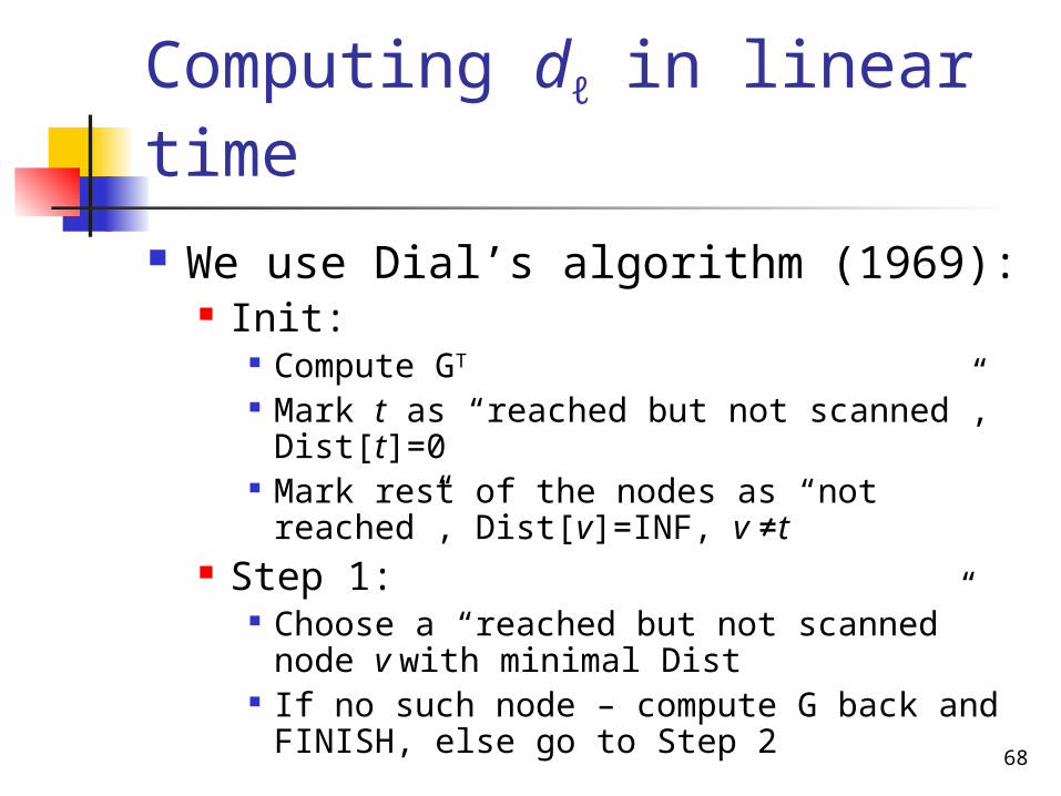
Computing dℓ in linear time We use Dial’s algorithm (1969):
Init: Compute GT
Mark t as “reached but not scanned”, Dist[t]=0
Mark rest of the nodes as “not reached”, Dist[v]=INF, v ≠t
Step 1: Choose a “reached but not scanned”
node v with minimal Dist If no such node – compute G back and
FINISH, else go to Step 2

69
Dial’s algorithm (cont.)
Step 2: For each (v,w) :
if Dist(w ) > Dist(v ) + ℓ(v,w), then Mark w as “reached but not scanned” Dist(w ) = Dist(v ) + ℓ(v,w) Add (v,w) to the output Remove all arcs (u,w) from the output, u ≠ w
Mark v as “reached and scanned” Go to Step 1

70
Dial’s algorithm Example
a b
d
ts
c
node
status
Dist
t RnS 0
s nR INF
a nR INF
b nR INF
c nR INF
d nR INF
G
GT
0
10
00
0
1
1
1
a b
d
ts
c0
10
00
0
1
1
1
1
1

71
Dial’s algorithm Example (cont.)
node
status
Dist
t RnS 0
s nR INF
a nR INF
b nR INF
c nR INF
d nR INF
Dist(b) > Dist(t) + ℓ(t,b)
a b
d
ts
c0
10
00
0
1
1
1
0RnS
1
distance
nodes
0
1
b

72
Dial’s algorithm Example (cont.)
node
status
Dist
t RnS 0
s nR INF
a nR INF
b RnS 0
c nR INF
d nR INF
Dist(d) > Dist(t) + ℓ(t,d)
a b
d
ts
c0
10
00
0
1
1
1
1RnS
RS1
distance
nodes
0 b
1d

73
Dial’s algorithm Example (cont.)
node
status
Dist
t RS 0
s nR INF
a nR INF
b RnS 0
c nR INF
d RnS 1
Dist(a) > Dist(b) + ℓ(b,a)1Rn
S
a b
d
ts
c0
10
00
0
1
1
11
distance
nodes
0 b
1 da
74
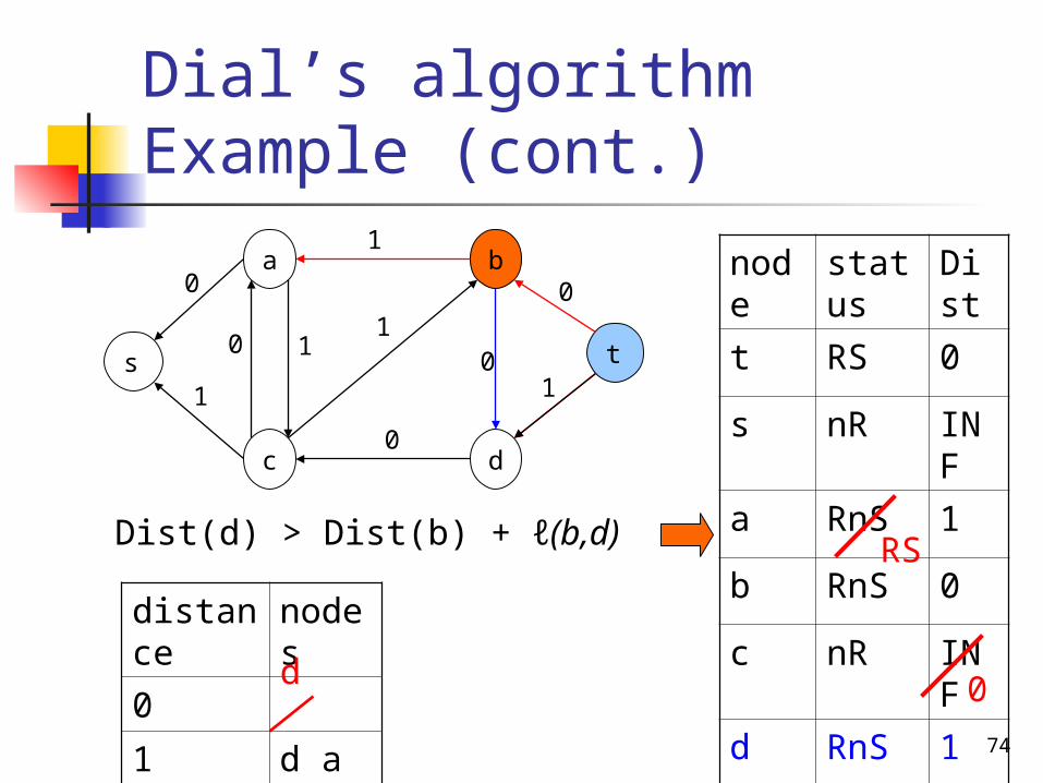
Dial’s algorithm Example (cont.)
node
status
Dist
t RS 0
s nR INF
a RnS 1
b RnS 0
c nR INF
d RnS 1
Dist(d) > Dist(b) + ℓ(b,d)
0
a b
d
ts
c0
10
00
0
1
1
11
distance
nodes
0
1 d a
d
RS

75
Dial’s algorithm Example (cont.)
node
status
Dist
t RS 0
s nR INF
a RnS 1
b RS 0
c nR INF
d RnS 0
Dist(c) > Dist(d) + ℓ(d,c)
0
a b
d
ts
c0
10
00
0
1
1
11
distance
nodes
0 d
1 a
cRnSRS

76
Dial’s algorithm Example (cont.)
node
status
Dist
t RS 0
s nR INF
a RnS 1
b RS 0
c RnS 0
d RS 0
Dist(s) > Dist(c) + ℓ(c,s)
1
a b
d
ts
c0
10
00
0
1
1
11
distance
nodes
0 c
1 as
RnS

77
Dial’s algorithm Example (cont.)
node
status
Dist
t RS 0
s RnS 1
a RnS 1
b RS 0
c RnS 0
d RS 0
Dist(a) > Dist(c) + ℓ(c,a)0
a b
d
ts
c0
10
00
0
1
1
11
distance
nodes
0
1 a s
aRS

78
Dial’s algorithm Example (cont.)
node
status
Dist
t RS 0
s RnS 1
a RnS 0
b RS 0
c RS 0
d RS 0
Dist(s) > Dist(a) + ℓ(a,s)
0
a b
d
ts
c0
10
00
0
1
1
11
distance
nodes
0 a
1 s
s
RS

79
Dial’s algorithm Example (cont.)
node
status
Dist
t RS 0
s RnS 0
a RS 0
b RS 0
c RS 0
d RS 0
Dist(s) > Dist(a) + ℓ(a,s)
a b
d
ts
c0
10
00
0
1
1
11
distance
nodes
0 s
1
RS

80
Dial’s algorithm Example (cont.)
node
status
Dist
t RS 0
s RS 0
a RS 0
b RS 0
c RS 0
d RS 0
a b
d
ts
c0
10
00
0
1
1
11
Final result:

81
Dial’s algorithm Running Time
Build GT – O(n+m) Each arc is examined once – O(m) By keeping bins for possible
distances, perform Step 1 in linear time – O(nU)
Total – O(m + nU)

82
References “Beyond the Flow Decomposition
Barrier”, A.V. Goldberg, Satish Rao “A Brief History Of Max-Flow”, R.
Khandekar, K.Talwar “The maximum flow problem”, I.
Hudson “Shortest-path forest with
topological ordering”, R.B. Dial


