Research ArticleBezier Curves Based Numerical Solutions ofDelay Systems with Inverse Time
F Ghomanjani1 M H Farahi1 A KJlJccedilman2 A V Kamyad1 and N Pariz3
1 Department of Mathematics Ferdowsi University of Mashhad Mashhad Iran2Department of Mathematics Universiti Putra Malaysia 43400 Serdang Selangor Malaysia3 Department of Control Faculty of Engineering Ferdowsi University of Mashhad Mashhad Iran
Correspondence should be addressed to A Kılıcman akilicupmedumy
Received 10 July 2013 Accepted 29 December 2013 Published 27 February 2014
Academic Editor Mufid Abudiab
Copyright copy 2014 F Ghomanjani et al This is an open access article distributed under the Creative Commons Attribution Licensewhich permits unrestricted use distribution and reproduction in any medium provided the original work is properly cited
This paper applied for the first time the Bernsteinrsquos approximation on delay differential equations and delay systems with inversedelay that models these problems The direct algorithm is given for solving this problem The delay function and inverse timefunction are expanded by the Bezier curves The Bezier curves are chosen as piecewise polynomials of degree 119899 and the Beziercurves are determined on any subinterval by 119899 + 1 control points The approximated solution of delay systems containing inversetime is derived To validate accuracy of the present algorithm some examples are solved
1 Introduction
Delay differential equations (DDEs) differ fromODEs in thatthe derivative at any time depends on the solution at priortimes (and in the case of neutral equations on the derivativeat prior times)
DDEs often arise when traditional pointwise model-ing assumptions are replaced by more realistic distributedassumptions for example when the birth rate of predatorsis affected by prior levels of predators or prey rather than byonly the current levels in a predator-prey model
Because the derivative (119905) depends on the solution atprevious time(s) it is necessary to provide an initial historyfunction to specify the value of the solution before time 119905 =
0 In many common models the history is a constant butnonconstant history functions are encountered routinely
For most problems there is a jump derivative discontinu-ity at the initial time In most models the DDE and the initialfunction are incompatible for some derivative order usuallythe first the left and right derivatives at 119905 = 0 are not equalDelay systems containing inverse time are an important classof systems
(119905) = 119909 (119905 minus 1) (0+
) = 1 (0minus
) = 0 (1)
A fascinating property is how such derivative discontinuitiesare propagated in time For the equation and history justdescribed for example the initial first discontinuity is propa-gated as a second degree discontinuity at time 119905 = 1 as a thirddegree discontinuity at time 119905 = 2 and more generally as adiscontinuity in the (119899 + 1)st derivative at time 119905 = 119899
Delay differential equations are type of differential equa-tions where the time derivatives at the current time dependon the solution and possibly its derivatives at previous times(see [1ndash4])
The basic theory concerning the stable factors for exam-ple existence and uniqueness of solutions was presented in[1 3] Since then DDEs have been extensively studied inrecent decades and a great number of monographs have beenpublished including significant works on dynamics of DDEsby Hale and Lunel [5] and on stability by Niculescu [6] Theinterest in study of DDEs is caused by the fact that manyprocesses have time delays and have been models for betterrepresentations by systems of DDEs in science engineeringeconomics and so forth Such systems however are still notfeasible to actively analyze and control precisely thus thestudy of systems of DDEs has actively been conducted overthe recent decades (see [7ndash10])
Hindawi Publishing CorporationMathematical Problems in EngineeringVolume 2014 Article ID 602641 16 pageshttpdxdoiorg1011552014602641
2 Mathematical Problems in Engineering
Wu et al [11] developed a computational method forsolving an optimal control problem which is governed bya switched dynamical system with time delay Kharatishivili[12] has approached this problem by extending Pontryaginrsquosmaximum principle to time delay systems The actual solu-tion involves a two-point boundary-value problem in whichadvances and delays are presented In addition this solutiondoes not yield a feedback controller Optimal-time controlof delay systems has been considered by Oguztoreli [13]who obtained several results concerning bang-bang controlswhich are parallel to those of LaSalle [14] for nondelay sys-tems For a time-invariant system with an infinite upper limitin the performance measure Krasovskii [15] has developedthe forms of the controller and the performance measureRoss [16] has obtained a set of differential equations for theunknowns in the forms of Krasovskii However Rossrsquos resultsare not applicable to time-varying systems with a finite limitin the performance measure
Basin and Perez [17] presented an optimal regulator fora linear system with multiple state and input delays and aquadratic criterion The optimal regulator equations wereobtained by reducing the original problem to the linear-quadratic regulator design for a system without delays (see[17 18])
This paper aims at solving delay systems containinginverse time of the following form
x (119905) = 119860 (119905) x (119905) + 119862 (119905) (1199091(119905 minus 1205911) sdot sdot sdot 119909
are matrix functions We need to imposethe continuity condition on x(119905) and its first derivative wherethese constraints appeared in Section 2
Piecewise polynomial functions are often used to repre-sent the approximate solution in the numerical solution ofdifferential equations (see [19ndash22]) B-splines due to numer-ical stability and arbitrary order of accuracy have becomepopular tools for solving differential equations (where Bezierform is a special case of B-splines)There aremany papers andbooks dealing with the Bezier curves or surface techniques
Harada and Nakamae [23] Nurnberger and Zeilfelder[24] used the Bezier control points in approximated dataand functions Zheng et al [22] proposed the use of controlpoints of the Bernstein-Bezier form for solving differentialequations numerically and also Evrenosoglu and Somali [25]used this approach for solving singular perturbed two-pointboundary-value problems The Bezier curves are used insolving partial differential equations as well Wave and Heat
equations are solved in Bezier form (see [26ndash29]) the Beziercurves are used for solving dynamical systems (see [30]) andalso the Bezier control pointsmethod is used for solving delaydifferential equation (see [31 32])
TheBezier curvesmethodwas presentedwhichwas statedfor solving the optimal control systems with pantographdelays (see [33]) The method was computationally attractiveand also reduced the CPU time and the computer memoryand at the same time keeps the accuracy of the solution Thealgorithm had been successfully applied to the pantographequations Comparing with other methods the results ofnumerical examples demonstrated that thismethodwasmoreaccurate than some existing methods (see [33])
Using Bezier curve Ghomanjani et al [34] had usedleast square method for numerical solutions of time-varyinglinear optimal control problems with time delays in state andcontrol
Some other applications of the Bezier functions andcontrol points are found in [35ndash37] that are used in computeraided geometric design and image compression
The use of the Bezier curves is a novel idea for solvingdelay systems containing inverse time The approach used inthis paper reduces the CPU time and the computer memorycomparing with existingmethods (see the numerical results)Although the method is very easy to use and straightforwardthe obtained results are satisfactory (see the numericalresults) We suggest a technique similar to the one used in[22 25] for solving delay systems containing inverse timeThecurrent paper is organized as follows
In Section 2 Function approximation will be introducedConvergence analysis will be stated in Section 3 In Section 4some numerical examples are solved which show the effi-ciency and reliability of the method Finally Section 5 willgive a conclusion briefly
2 Function Approximation
Divide the interval [1199050 119905119891] into a set of grid points such that
minus 119905) 1 le 119894 le 119901 is the 119894thcomponent of (1199091198962minus119895
1(119905119891minus 119905) sdot sdot sdot 119909
1198962minus119895
119901(119905119891minus 119905))119879 where (119905
119891minus 119905) isin
[1199051198962minus119895minus1
1199051198962minus119895] Also
119896119894
1=
120591119894
ℎ
120591119894
ℎ
isin N
([
120591119894
ℎ
] + 1)
120591119894
ℎ
notin N
1 le 119894 le 119901
1198962=
119905119891
ℎ
119905119891
ℎ
isin N
([
119905119891
ℎ
] + 1)
119905119891
ℎ
notin N
(5)
where [120591119894ℎ] and [119905
119891ℎ] denote the integer part of 120591
119894ℎ and
119905119891ℎ respectivelyOur strategy is to use Bezier curves to approximate the
solutions x119895(119905) and u
119895(119905) by k
119895(119905) and w
119895(119905) respectively
where k119895(119905) and w
119895(119905) are given below Individual Bezier
curves that are defined over the subintervals are joinedtogether to form the Bezier spline curves For 119895 = 1 2 119896define the Bezier polynomials of degree 119899 that approximaterespectively the actions of x
119895(119905) and u
119895(119905) over the interval
[119905119895minus1
119905119895] as follows
k119895(119905) =
119899
sum
119903=0
a119895119903119861119903119899
(
119905 minus 119905119895minus1
ℎ
)
w119895(119905) =
119899
sum
119903=0
b119895119903119861119903119899
(
119905 minus 119905119895minus1
ℎ
)
(6)
where
119861119903119899
(
119905 minus 119905119895minus1
ℎ
) = (
119899
119903)
1
ℎ119899(119905119895minus 119905)
119899minus119903
(119905 minus 119905119895minus1
)
119903
(7)
is the Bernstein polynomial of degree 119899 over the interval[119905119895minus1
119905119895] a119895119903and b119895
119903are respectively 119901 and 119898 ordered vectors
from the control points (see [22]) By substituting (6) in (4)1198771119895
(119905) for 119905 isin [119905119895minus1
119905119895] can be defined as follows
1198771119895
(119905) = k119895(119905) minus 119860 (119905) k
119895(119905)
minus 119862 (119905) (Vminus1198961
1+119895
1(119905 minus 1205911) sdot sdot sdot Vminus119896
where the so-called b119895119903(119903 = 0 1 119899 minus 1 119899) is an 119898 ordered
vectorNow the residual function can be defined in 119878
119895as follows
119877119895= int
119905119895
119905119895minus1
100381710038171003817100381710038171198771119895
(119905)
10038171003817100381710038171003817
2
119889119905 (13)
where sdot is the Euclidean norm (recall that 1198771119895
(119905) is a 119901
vector where 119905 isin 119878119895)
Our aim is to solve the following problem over 119878 =
⋃119896
119895=1119878119895
min119896
sum
119895=1
119877119895
st a119895119899= a119895+10
(a119895119899minus a119895119899minus1
) = (a119895+11
minus a119895+10
) 119895 = 1 2 119896 minus 1
(14)
The mathematical programming problem (14) can be solvedby many subroutine algorithms Here we used Maple 12 tosolve this optimization problem
4 Mathematical Problems in Engineering
Remark 2 Consider the following boundary value problem
y (119905) = 119877 (119905) y (119905) + 119876 (119905) y (119905 minus 120572) + 119878 (119905) z (119905) + a (119905)
z (119905) = 119881 (119905) y (119905) + 119870 (119905) z (119905 + 120572) + 119882 (119905) z (119905) + b (119905)
y (1199050) = y0
y (119905) = 120601 (119905) 119905 isin [minus120572 1199050)
z (119905119891) = z0
z (119905) = 120595 (119905) 119905 isin (119905119891 119905119891+ 120572]
(15)
where y(119905) z(119905) a(119905) b(119905) 120601(119905) and 120595(119905) are the vectorsof appropriate dimensions 119877(119905) 119876(119905) 119878(119905) 119881(119905) 119870(119905) and119882(119905) are the matrices of appropriate dimensions and 120572 isnonnegative constant time delay
Let
x (119905) = [y(119905)119879 z(119905119891minus 119905)
119879
]
119879
(16)
where 119879 is the transpose then
x (119905) = [y119879 (119905) minusz119879 (119905119891minus 119905)]
119879 (17)
satisfies that
x (119905) = 119860 (119905) x (119905) + 119862 (119905) x (119905 minus 120572)
+ 119863 (119905) x (119905119891minus 119905) + u (119905) 119905 isin [119905
0 119905119891]
x (1199050) = x0= [y1198790
z1198790]
119879
(18)
where
119860 (119905) = 119864(2)
11otimes 119877 (119905) minus 119864
(2)
22otimes 119882(119905
119891minus 119905)
119862 (119905) = 119864(2)
11otimes 119876 (119905) minus 119864
(2)
22otimes 119870 (119905
119891minus 119905)
119863 (119905) = 119864(2)
12otimes 119878 (119905) minus 119864
(2)
21otimes 119881 (119905
119891minus 119905)
u (119905) = [a119879 (119905) minusb119879 (119905119891minus 119905)]
119879
(19)
where119864(119891)119894119895
is the119891times119891matrix with 1 at its entry (119894 119895) and zeroselsewhere and otimes is Kronecker product (see eg [4 38 39])
Remark 3 Now the following delay differential equation canbe considered
(119905) = 119891 (119905 119909 (119905) 119909 (119905 minus 120591 (119905 119909 (119905)))) 119905 ge 0 (20)
where 120582 equiv inf119905 minus 120591(119905 119906) 119905 ge 0 119906 isin R In the case when 120582 isnot finite [minus120582 0] denotes the interval (minusinfin 0]
Furthermore we assume that
120591 (119905 119906) ge 0 forall119905 ge 0 119906 isin R (22)
that is (20) is a delay differential equationThe existence anduniqueness of the solution of initial value problem (20)-(21)was stated in [40]
Equation (20) is converted into a nonlinear programmingproblem (NLP) by applying Bezier control points methodwhereas the MATLAB optimization routine FMINCON isused for solving resulting NLP Numerical example showsthat the proposed method is efficient and very easy to use
Remark 4 Now we limit ourselves to consider the followingnonlinear delay differential equation in the type
119909 (119905) = 120601 (119905) 119905 le 1199050
(24)
where the differential operator 119871 is defined by 119871(sdot) =
119889119899(sdot)119889119905119899
3 Convergence Analysis
In this section without loss of generality we analyze theconvergence of the control-point-based method applied tothe problem (2) with time delay in state when 119901 = 119898 = 1and the time interval is [0 1] So the following problem isconsidered
119871(119909 (119905) 119906 (119905) 119909 (119905 minus 120591) 119909 (1 minus 119905)
119889119909 (119905)
119889119905
) =
119889119909 (119905)
119889119905
minus 119860 (119905) 119909 (119905) minus 119862 (119905) 119909 (119905 minus 120591) minus 119866 (119905) 119906 (119905)
minus 119863 (119905) 119909 (1 minus 119905) = 119865 (119905) 119905 isin [0 1]
where 119909(119905) isin 119877 119906(119905) isin 119877 and 119886 119887 1198861are given real numbers
and 119860(119905) 119862(119905) 119866(119905) 119863(119905) and 119865(119905) are known polynomialsfor 119905 isin [0 1] The constant time delay 120591 is nonnegative
Without loss of generality we consider the interval [0 1]instead of [119905
0 119905119891] since the variable 119905 can be changed with the
new variable 119911 by 119905 = (119905119891minus 1199050)119911 + 1199050where 119911 isin [0 1]
Lemma 5 For a polynomial in Bezier form
119909 (119905) =
1198991
sum
119894=0
1198861198941198991
1198611198941198991(119905) (26)
we have
sum1198991
119894=01198862
1198941198991
1198991+ 1
ge
sum1198991+1
119894=01198862
1198941198991+1
1198991+ 2
ge sdot sdot sdot
ge
sum1198991+1198981
119894=01198862
1198941198991+1198981
1198991+ 1198981+ 1
997888rarr int
1
0
1199092
(119905) 119889119905 1198981997888rarr +infin
(27)
Mathematical Problems in Engineering 5
where 1198861198941198991+1198981
is the Bezier coefficient of 119909(119905) after degree-elevating to degree 119899
1+ 1198981
Proof See [22 page 245]
The convergence of the approximate solution could bedone in two ways
(1) degree raising the Bezier polynomial approximation(2) subdivision of the time interval
In the following the convergence in each case canbe proven although in numerical examples we used onlysubdivision case (see [32])
31 Degree Raising
Theorem 6 If the problem (25) with inverse time in state hasa unique 119862
1 continuous trajectory solution 119909 1198620 continuouscontrol solution 119906 then the approximate solution obtained bythe control-point-based method converges to the exact solution(119909 119906) as the degree of the approximate solution tends to infinity
Proof Given an arbitrary small positive number 120598 gt
0 by the Weierstrass theorem (see [41]) one can easilyfind polynomials 119876
(119905) do not satisfy the boundaryconditions After a small perturbation with linear and con-stant polynomials 120572119905 + 120573 120574 respectively for 119876
11198731
(119905) and11987621198732
(119905) we can obtain polynomials 11987511198731
(119905) = 11987611198731
(119905) +
(120572119905 + 120573) and 11987521198732
(119905) = 11987621198732
(119905) + 120574 such that 11987511198731
(119905) satisfiesthe boundary conditions 119875
11198731
(0) = 119886 11987511198731
(1) = 119887 and11987521198732
(0) = 1198861Thus119876
11198731
(0)+120573 = 119886 and11987611198731
(1)+120572+120573 = 119887By using (28) one has
10038171003817100381710038171003817119887 minus 11987611198731(1)
10038171003817100381710038171003817infin
=1003817100381710038171003817120572 + 120573
1003817100381710038171003817infin
le
120598
16
10038171003817100381710038171003817119886 minus 119876
The last inequality in (41) is obtained by Lemma 5 where119862 isa constant positive number Now
(119909 (119905) 119906 (119905)) minus (119909 (119905) 119906 (119905)) le
119862
1198982+ 1
1198982
sum
119894=0
1198882
1198941198982
le
119862
1198982+ 1
1198982
sum
119894=0
1198892
1198941198982
le
119862
1198981+ 1
1198981
sum
119894=0
1198892
1198941198981
le 119862 (120598 + 1198622
11205982
)
= 1205981 1198981ge 119872
(42)
where the last inequality in (42) comes from (36) Thiscompletes the proof
32 Subdivision
Theorem 7 Let (119909 119906) be the approximate solution of theproblem (25) with inverse time obtained by the subdivisionscheme of the control-point-based method If (25) has a uniquesolution (119909 119906) and (119909 119906) is smooth enough so that the cubicspline 119879(119909 119906) interpolates to (119909 119906) and converges to (119909 119906) inthe order 119874(ℎ
119902) (119902 gt 2) where ℎ is the maximal width of all
subintervals then (119909 119906) converges to (119909 119906) as ℎ rarr 0
Proof We first impose a uniform partition prod119889= ⋃119894[119905119894 119905119894+1
]
on the interval [0 1] as 119905119894= 119894119889 where 119889 = 1(119899
1+ 1)
Mathematical Problems in Engineering 7
Let 119868119889(119909(119905) 119906(119905) 119909(119905 minus 120591) 119909(1 minus 119905) 119889119909(119905)119889119905) be the cubic
spline over prod119889which is interpolating to (119909 119906) Then for an
arbitrary small positive number 120598 gt 0 there exists a 1205751gt 0
119889(119909(119905) 119906(119905) 119909(119905 minus
120591) 119909(1 minus 119905) 119889119909(119905)119889119905)) = 119871(119868119889(119909(119905) 119906(119905) 119909(119905 minus 120591) 119909(1 minus
119905) 119889119909(119905)119889119905)) minus 119865(119905) be the residual For each subinterval[119905119894 119905119894+1
] 119877(119868119889(119909(119905) 119906(119905) 119909(119905 minus 120591) 119909(1 minus 119905) 119889119909(119905)119889119905))
is a polynomial On each interval [119905119894 119905119894+1
119909 (119905) 119906 (119905) 119909 (119905 minus 120591)
119909 (1 minus 119905)
119889119909 (119905)
119889119905
))119889119905 + 120598
lt (119897 + 1) 1205982
+ 120598
(47)
Now combining the partitionsprod119889and allprod
119894ℎgives a denser
partition with the length ℎ for each subinterval Suppose(119909(119905) 119906(119905)) is the approximate solution by the control-point-based method with respect to this partition and denote theresidual over [119905
119894119895minus1 119905119894119895] by
119877(119909 (119905) 119906 (119905) 119909 (119905 minus 120591) 119909 (1 minus 119905)
119889119909 (119905)
119889119905
)
= 119871(119909 (119905) 119906 (119905) 119909 (119905 minus 120591) 119909 (1 minus 119905)
119889119909 (119905)
119889119905
) minus 119865 (119905)
=
119897
sum
1199011=0
119888119894119895
1199011
1198611199011119897(119905)
(48)
Define the following norm for difference approximate solu-tion (119909(119905) 119906(119905)) and exact solution (119909(119905) 119906(119905))
(119909 (119905) 119906 (119905)) minus (119909 (119905) 119906 (119905))
119905 minus 2 + radic4 minus 2119905 0 le 119905 le 2
0 119905 gt 2
(66)
12 Mathematical Problems in Engineering
The solution of this problem is
119909 (119905) =
(119905 minus 2)2
4
0 le 119905 le 2
0 119905 gt 2
(67)
By choosing 119896 = 1 and 119899 = 7 (degree raising) we obtain thefollowing solution
119909 (119905) = 1 minus 1000000002119905 + 3207267830 times 10minus9
1199056
+ 02500000112 times 1199052
minus 3416339151 times 10minus10
1199057
minus 1204800000 times 10minus8
1199055
minus 2304000000 times 10minus8
1199053
+ 2296000000 times 10minus8
1199054
(68)
In Table 5 exact numerical results of this method method in[40] error of presented method and error of the method in[40] are shown respectively
Example 14 Consider the following LDDE described by
1198893119909 (119905)
1198891199053
= minus119909 (119905) minus 119909 (119905 minus 03) + 119890minus119905+03
0 le 119905 le 1 (69)
with the initial conditions
119909 (0) = 1
119889119909 (0)
119889119905
= minus1
1198892119909 (0)
1198891199052
= 1 119909 (119905) = 119890minus119905
119905 le 0
(70)
where the exact solution of this example is 119909(119905) = 119890minus119905 Here
this problem is solved by choosing 119896 = 10 and 119899 = 3The graph of error is shown in Figure 5 and the followingapproximate solution 119909(119905) is found
119909 (119905) =
1 minus 119905 + 051199052minus 0172928119905
3 119905 isin [0 01]
09999767558 minus 0999302674119905 + 0493026741199052minus 01496838119905
3 119905 isin [01 02]
09998081522 minus 0996773576119905 + 0480381041199052minus 01286073119905
3 119905 isin [02 03]
09992953871 minus 0991645877119905 + 0463288531199052minus 01096154119905
3 119905 isin [03 04]
09982244623 minus 0983613861119905 + 0443208291199052minus 00928817119905
3 119905 isin [04 05]
09964070488 minus 0972709334119905 + 0421399141199052minus 00783422119905
3 119905 isin [05 06]
09937493164 minus 09594206119905 + 0399251141199052minus 00660377119905
3 119905 isin [06 07]
09903114379 minus 0944686777119905 + 0378202731199052minus 00560146119905
3 119905 isin [07 08]
09863822587 minus 0929952279119905 + 0359784511199052minus 00483403119905
3 119905 isin [08 09]
09825547252 minus 0917193744119905 + 0345608261199052minus 00430898119905
3 119905 isin [09 1]
(71)
Example 15 Consider the second-order linear decay differ-ential equation
(119905) =
3
4
119909 (119905) + 119909 (
119905
2
) minus 1199052
+ 2 0 le 119905 le 1
119909 (0) = 0 (0) = 0
(72)
The exact solution of this problem is 119909(119905) = 1199052 Here this
problem is solved by choosing 119896 = 1 and 119899 = 7 The followingapproximate solution 119909(119905) is found
119909 (119905) = 18828480001199052
minus 50726239991199053
+ 15564000001199054
minus 28142400001199055
+ 30840000001199056
minus 1199059
+ 71199058
minus 006182400000119905
minus 20010000001199057
(73)
In Table 6 exact numerical results of this method error ofpresentedmethod and error of themethod in [43] are shownrespectively
5 Conclusions
Using the Bezier curves the general algorithm is providedfor the delay systems containing inverse time Numericalexamples show that the proposedmethod is efficient and veryeasy to use
Appendix
In this Appendix we specify the derivative of Bezier curveBy (6) we have
k119895(119905) =
119899
sum
119894=0
119886119895
119894119861119894119899
(119905) 119905 isin [0 1] (A1)
where 119861119894119899(119905) = (119899119894(119899 minus 119894))119905
119894(1 minus 119905)
119899minus119894Now we have (see [44])
119889119861119894119899
(119905)
119889119905
= 119899 (119861119894minus1119899minus1
(119905) minus 119861119894119899minus1
(119905)) 0 le 119894 le 119899 (A2)
Mathematical Problems in Engineering 13
minus02
minus04
minus06
minus08
minus1
minus06 minus04 minus02 0 02 04 06 08 1
Approximate x1(t)Exact x1(t)
t
Figure 3The graph of approximated trajectory 1199091(119905) for Example 2
5
4
3
2
minus06 minus04 minus02 0 02 04 06 08 1
t
Approximate x2(t)Exact x2(t)
Figure 4The graph of approximated trajectory 1199092(119905) for Example 2
where 119861minus1119899minus1
(119905) = 119861119899119899minus1
(119905) = 0 and
119861119894minus1119899minus1
(119905) =
(119899 minus 1)
(119894 minus 1) (119899 minus 119894)
119905119894minus1
(1 minus 119905)119899minus119894
119861119894119899minus1
(119905) =
(119899 minus 1)
119894 (119899 minus 119894 minus 1)
119905119894
(1 minus 119905)119899minus119894minus1
(A3)
00014
00012
00010
00008
00006
00004
00002
0
0 02 04 06 08 1
t
Error
Figure 5 The graph of error for Example 7
By using (A2) the first derivative k119895(119905) is shown as
119889k119895(119905)
119889119905
=
119899minus1
sum
119894=1
119899a119895119894119861119894minus1119899minus1
(119905) minus
119899minus1
sum
119894=0
119899a119895119894119861119894119899minus1
(119905)
=
119899minus1
sum
119894=0
119899a119895119894+1
119861119894119899minus1
(119905) minus
119899minus1
sum
119894=0
119899a119895119894119861119894119899minus1
(119905)
=
119899minus1
sum
119894=0
119861119894119899minus1
(119905) 119899 a119895119894+1
minus a119895119894
(A4)
Now we specify the procedure of derivation of (10) from (9)By (6) we have
k119895(119905) = (
119899
0) a1198950
1
ℎ119899(119905119895minus 119905)
119899
+ sdot sdot sdot + (
119899
119899) a119895119899
1
ℎ119899(119905 minus 119905119895minus1
)
119899
k119895+1
(119905) = (
119899
0) a119895+10
1
ℎ119899(119905119895+1
minus 119905)
119899
+ sdot sdot sdot + (
119899
119899) a119895+1119899
1
ℎ119899(119905 minus 119905119895)
119899
(A5)
by substituting 119905 = 119905119895into (A5) one has
k119895(119905119895) = a119895119899
1
ℎ119899(119905119895minus 119905119895minus1
)
119899
k119895+1
(119905119895) = a119895+10
1
ℎ119899(119905119895+1
minus 119905119895)
119899
(A6)
14 Mathematical Problems in Engineering
Table 1 Exact and estimated values of 1199091(119905) for Example 3
From (A4) the first derivatives of k119895(119905) and k
119895+1(119905) are
respectively
119889k119895(119905)
119889119905
=
119899minus1
sum
119894=0
119861119894119899minus1
(119905) 119899 (a119895119894+1
minus a119895119894)
=
119899minus1
sum
119894=0
(
119899 minus 1
119894) (119905119895minus 119905)
119899minus1minus119894
(119905 minus 119905119895minus1
)
119894
times
1
ℎ119899119899 (a119895119894+1
minus a119895119894)
= (
119899 minus 1
0) 119899 (a119895
1minus a1198950)
1
ℎ119899(119905119895minus 119905)
119899minus1
+ sdot sdot sdot + (
119899 minus 1
119899 minus 1) 119899 (a119895
119899minus a119895119899minus1
)
times
1
ℎ119899(119905 minus 119905119895minus1
)
119899minus1
119889k119895+1
(119905)
119889119905
=
119899minus1
sum
119894=0
(
119899 minus 1
119894) (119905119895+1
minus 119905)
119899minus1minus119894
(119905 minus 119905119895)
119894
times
1
ℎ119899119899 (a119895+1119894+1
minus a119895+1119894
)
= (
119899 minus 1
0) 119899 (a119895+1
1minus a119895+10
)
1
ℎ119899(119905119895+1
minus 119905)
119899minus1
+ sdot sdot sdot + (
119899 minus 1
119899 minus 1) 119899 (a119895+1
119899minus a119895+1119899minus1
)
times
1
ℎ119899(119905 minus 119905119895)
119899minus1
(A8)
By substituting 119905 = 119905119895into (A8) we have
119889k119895(119905119895)
119889119905
= 119899 (a119895119899minus a119895119899minus1
)
1
ℎ119899(119905119895minus 119905119895minus1
)
119899minus1
119889k119895+1
(119905119895)
119889119905
= 119899 (a119895+11
minus a119895+10
)
1
ℎ119899(119905119895+1
119905119895)
119899minus1
(A9)
and to preserve the continuity of the first derivative of Beziercurves at nodes by equalizing (A9) we have
(a119895119899minus a119895119899minus1
) (119905119895minus 119905119895minus1
)
119899minus1
= (a119895+11
minus a119895+10
) (119905119895+1
minus 119905119895)
119899minus1
(A10)
where it shows the equality (10)
Mathematical Problems in Engineering 15
Table 4 Exact and estimated values of 119909(119905) for Example 5
119905 Exact Presented method Method in [40] Error of presented method Error of the method in [40]05 110468992792789 110468992817860 11451 250709000000000 times 10
minus10
12232 times 10minus3
10 153790187962670 153790188062000 15361 993297 times 10minus10
17685 times 10minus3
14 193790187962670 193768171138582 19361 0220168240883 times 10minus3
17685 times 10minus3
15 203790187962670 203790188078453 20362 1157827 times 10minus9
16125 times 10minus3
20 253790187962670 253790188032000 25870 693297 times 10minus10
49096 times 10minus2
Table 5 Exact and estimated values of 119909(119905) for Example 6
119905 Exact Presented method Method in [40] Error of presented method Error of the method in [40]10 025 0250000000017634 0250013 17634 times 10
minus11
128346 times 10minus5
20 00 00 526486 times 10minus7 00 526486 times 10
minus7
Table 6 Exact and estimated values of 119909(119905) for Example 8
119905 Exact Presented method Error Of presented method Error of the method in [43]02 004 00400000000049152 49152 times 10
minus12
173 times 10minus6
04 016 01600000000193540 19354 times 10minus11
110 times 10minus5
06 036 03600000000221180 22118 times 10minus11
126 times 10minus4
08 064 06400000000073730 7373 times 10minus12
707 times 10minus4
Conflict of Interests
The authors declare that they have no conflict of interestsregarding publication of this paper
Acknowledgment
The authors would like to thank the anonymous reviewersfor their careful reading constructive comments and nicesuggestions which have improved the paper very much
References
[1] G Adomian and R Rach ldquoNonlinear stochastic differentialdelay equationsrdquo Journal of Mathematical Analysis and Appli-cations vol 91 no 1 pp 94ndash101 1983
[2] J Baranowski ldquoLegendre polynomial approximations of timedelay systemsrdquo in Proceedings of the 12th International PhDWorkshop p 2326 2010
[3] F Maghami Asl and A G Ulsoy ldquoAnalysis of a system oflinear delay differential equationsrdquo Journal of Dynamic SystemsMeasurement and Control Transactions of the ASME vol 125no 2 pp 215ndash223 2003
[4] X T Wang ldquoNumerical solution of delay systems containinginverse time by hybrid functionsrdquo Applied Mathematics andComputation vol 173 no 1 pp 535ndash546 2006
[5] J K Hale and S M V Lunel Introduction to FunctionalDifferential Equations Springer New York NY USA 1993
[6] S I Niculescu Delay Effects on Stability a Robust ControlApproach Springer New York NY USA 2001
[7] D H Eller and J I Aggarwal ldquoOptimal control of linear time-delay systemsrdquo IEEE Transactions on Automatic Control vol 14no 14 pp 678ndash687 1969
[8] L Gollmann D Kern and H Maurer ldquoOptimal controlproblems with delays in state and control variables subject to
mixed control-state constraintsrdquo Optimal Control Applicationsand Methods vol 30 no 4 pp 341ndash365 2009
[9] N N Krasovskii ldquoOptimal processes in systems with time lagsrdquoin Proceedings of the 2nd International Conference of Interna-tional Federation of Automatic Control Basel Switzerland 1963
[10] R Loxton K L Teo and V Rehbock ldquoAn optimizationapproach to state-delay identificationrdquo IEEE Transactions onAutomatic Control vol 55 no 9 pp 2113ndash2119 2010
[11] C Wu K L Teo R Li and Y Zhao ldquoOptimal control ofswitched systems with time delayrdquoApplied Mathematics Lettersvol 19 no 10 pp 1062ndash1067 2006
[12] G L Kharatishivili ldquoThe maximum principle in the theoryof optimal processes with time lagsrdquo Doklady Akademii NaukSSSR vol 136 no 1 1961
[13] M N Oguztoreli ldquoA time optimal control problem for systemsdescribed by differential difference equationsrdquo SIAM Journal ofControl vol 1 no 3 pp 290ndash310 1963
[14] J P LaSalle ldquoThe time optimal control problemrdquo in Contribu-tions to the Theory of Nonlinear Oscillations vol 5 pp 1ndash24Princeton University Press Princeton NJ USA 1960
[15] N N Krasovskii ldquoOn the analytic construction of an optimalcontrol in a system with time lagsrdquo Prikladnaya Matematika iMekhanika vol 26 no 1 pp 50ndash67 1962
[16] D W Ross Optimal control of systems described by differentialdifference equations [PhD thesis] Department of ElectricalEnergy Stanford University Stanford Calif USA 1968
[17] M Basin and J Perez ldquoAn optimal regulator for linear systemswith multiple state and input delaysrdquo Optimal Control Applica-tions and Methods vol 28 no 1 pp 45ndash57 2007
[18] M Basin and J Rodriguez-Gonzalez ldquoOptimal control forlinear systems with multiple time delays in control inputrdquo IEEETransactions onAutomatic Control vol 51 no 1 pp 91ndash97 2006
[19] M Heinkenschloss ldquoA time-domain decomposition iterativemethod for the solution of distributed linear quadratic optimalcontrol problemsrdquo Journal of Computational and Applied Math-ematics vol 173 no 1 pp 169ndash198 2005
16 Mathematical Problems in Engineering
[20] H Juddu ldquoSpectral method for constrained linear-quaraticoptimal controlrdquoMathematics Computers in Simulation vol 58pp 159ndash169 2002
[21] R Winkel ldquoGeneralized bernstein polynomials and Beziercurves an application of umbral calculus to computer aidedgeometric designrdquoAdvances in AppliedMathematics vol 27 no1 pp 51ndash81 2001
[22] J Zheng T W Sederberg and R W Johnson ldquoLeast squaresmethods for solving differential equations using Bezier controlpointsrdquo Applied Numerical Mathematics vol 48 no 2 pp 237ndash252 2004
[23] K Harada and E Nakamae ldquoApplication of the Bezier curve todata interpolationrdquo Computer-Aided Design vol 14 no 1 pp55ndash59 1982
[24] G Nurnberger and F Zeilfelder ldquoDevelopments in bivariatespline interpolationrdquo Journal of Computational and AppliedMathematics vol 121 no 1 pp 125ndash152 2000
[25] M Evrenosoglu and S Somali ldquoLeast squares methods for solv-ing singularly perturbed two-point boundary value problemsusing Bezier control pointsrdquo Applied Mathematics Letters vol21 no 10 pp 1029ndash1032 2008
[26] J V Beltran and J Monterde ldquoBezier solutions of the waveequationrdquo in Computational Science and Its ApplicationsmdashICCSA 2004 vol 3044 of Lecture Notes in Computer Science pp631ndash640 2004
[27] R Cholewa A J Nowak R A Bialecki and L C WrobelldquoCubic Bezier splines for BEM heat transfer analysis of the 2-D continuous casting problemsrdquoComputationalMechanics vol28 no 3-4 pp 282ndash290 2002
[28] B Lang ldquoThe synthesis of wave forms using Bezier curves withcontrol point modulationrdquo in Proceedings of the 2nd CEMSResearch Student Conference Morgan Kaufamann 2002
[29] A T Layton and M Van de Panne ldquoA numerically efficientand stable algorithm for animating water wavesrdquo The VisualComputer vol 18 no 1 pp 41ndash53 2002
[30] M Gachpazan ldquoSolving of time varying quadratic optimal con-trol problems by using Bezier control pointsrdquo Computationaland Applied Mathematics vol 30 no 2 pp 367ndash379 2011
[31] F Ghomanjani and M H Farahi ldquoThe Bezier control pointsmethod for solving delay differential equationrdquo Intelligent Con-trol and Automation vol 3 no 2 pp 188ndash196 2012
[32] F Ghomanjani M H Farahi and M Gachpazan ldquoBeziercontrol points method to solve constrained quadratic optimalcontrol of time varying linear systemsrdquo Computational andApplied Mathematics vol 31 no 3 p 124 2012
[33] F Ghomanjani M H Farahi and A V Kamyad ldquoNumericalsolution of some linear optimal control systems with pan-tograph delaysrdquo IMA Journal of Mathematical Control andInformation 2013
[34] F Ghomanjani M H Farahi and M Gachpazan ldquoOptimalcontrol of time-varying linear delay systems based on the Beziercurvesrdquo Computational and Applied Mathematics 2013
[35] C-H Chu C C L Wang and C-R Tsai ldquoComputer aidedgeometric design of strip using developable Bezier patchesrdquoComputers in Industry vol 59 no 6 pp 601ndash611 2008
[36] G E Farin Curve and Surfaces for Computer Aided GeometricDesign Academic Press New York NY USA 1st edition 1988
[37] Y Q Shi and H Sun Image and Video Compression forMultimedia Engineering CRC 2000
[38] A Kılıcman ldquoOn the matrix convolutional products and theirapplicationsrdquo AIP Conference Proceedings vol 1309 pp 607ndash622 2010
[39] A Kılıcman and Z Al Zhour ldquoKronecker operational matricesfor fractional calculus and some applicationsrdquo Applied Mathe-matics and Computation vol 187 no 1 pp 250ndash265 2007
[40] I Gyori F Hartung and J Turi ldquoOn numerical solutionsfor a class of nonlinear delay equations with time-and state-dependent delaysrdquo in Proceedings of the World Congress ofNonlinear Analysts pp 1391ndash1402 New York NY USA 1996
[41] W Rudin Principles of Mathematical Analysis McGraw-Hill1986
[42] C Hwang and M-Y Chen ldquoAnalysis of time-delay systemsusing the Galerkin methodrdquo International Journal of Controlvol 44 no 3 pp 847ndash866 1986
[43] O A Taiwo andO S Odetunde ldquoOn the numerical approxima-tion of delay differential equations by a decompositionmethodrdquoAsian Journal of Mathematics and Statitics vol 3 no 4 pp 237ndash243 2010
[44] H Prautzsch W Boehm and M Paluszny Bezier and B-SplineTechniques Springer 2001


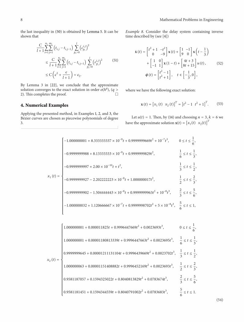


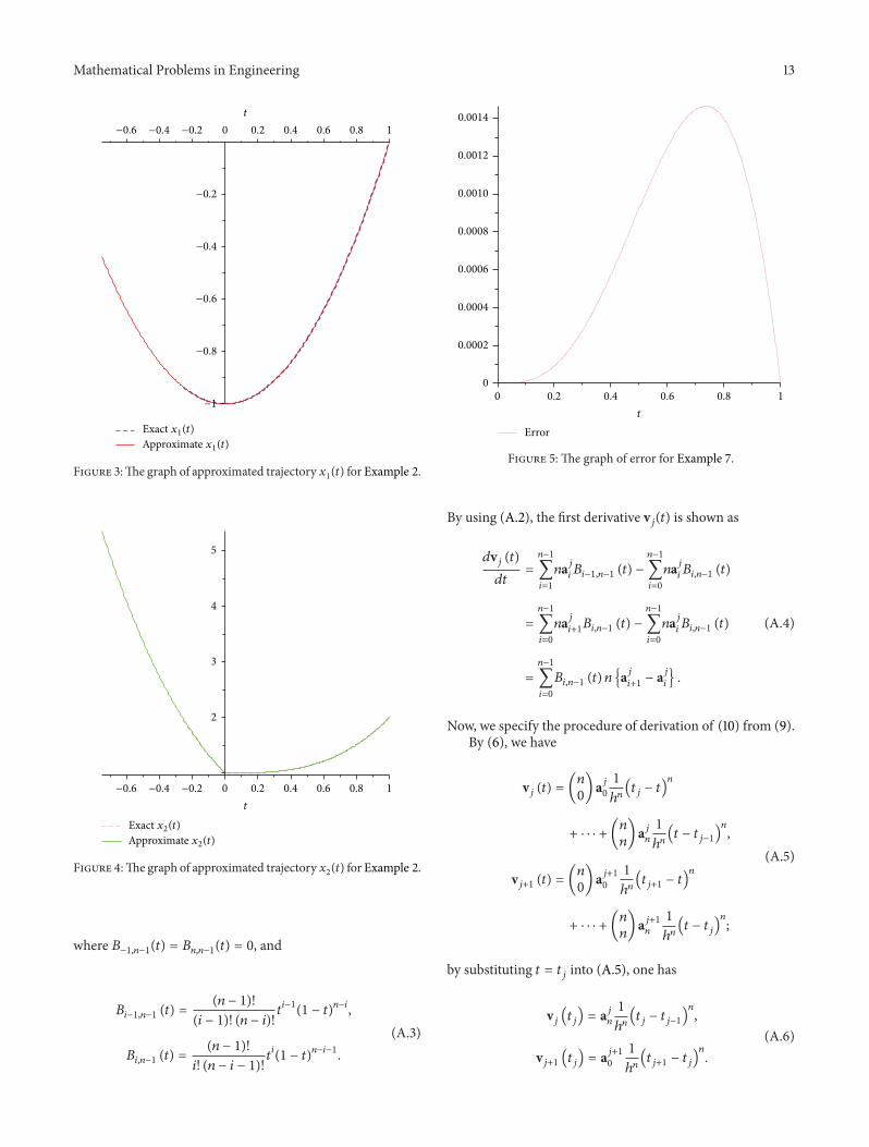
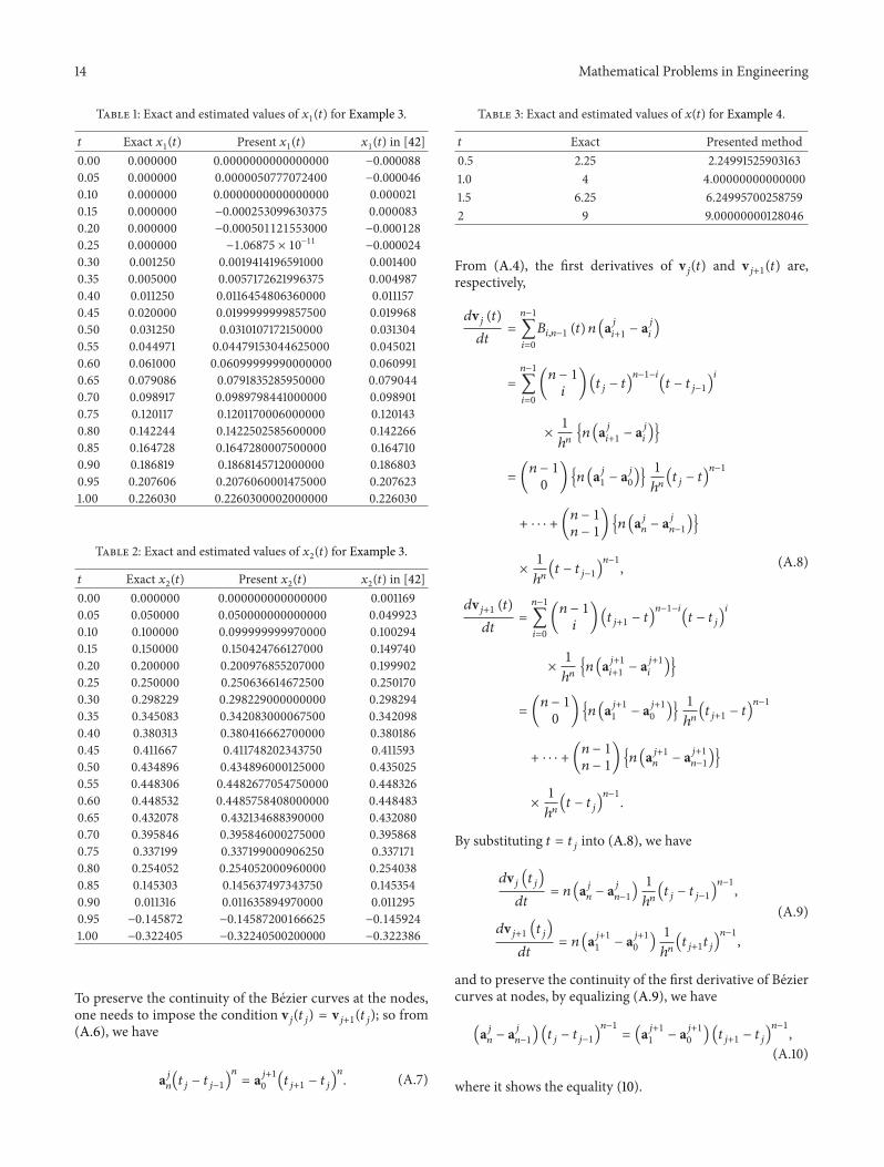


![Curves and Surfacesadair/CG/Notas Aula/Curvas/09-curves.pdf · Bezier Curves and Surfaces [Angel 10.1-10.6] Parametric Representations Cubic Polynomial Forms Hermite Curves Bezier](https://static.documents.pub/doc/80x56/5f72f8d58557ce2aea5f374f/curves-and-adaircgnotas-aulacurvas09-curvespdf-bezier-curves-and-surfaces.jpg)

