Computer Graphics and Imaging UC Berkeley CS184/284A, Spring 2017

Lecture 9:

Splines, Bezier Curves & Surfaces

Ren NgCS184/284A

Smooth Curves and Surfaces

So far we can make:

• Things with corners (lines, triangles, squares, …)

• Specialty shapes (circles, ellipses, …)

Many applications require designed, smooth shapes

• Camera paths, vector fonts, …

• Resampling filter functions

• CAD design, object modeling, …

Camera Paths

Flythrough of proposed Perth Citylink subway, https://youtu.be/rIJMuQPwr3E

Animation Curves

Maya Animation Tutorial: https://youtu.be/b-o5wtZlJPc

Vector Fonts

Baskerville font - represented as cubic Bézier splines

credit: Randall Branding

The Quick Brown Fox Jumps OverThe Lazy Dog ABCDEFGHIJKLMNOPQRSTUVWXYZ abcdefghijklmnopqrstuvwxyz 0123456789

CAD Design

3D Car Modeling with Rhinoceros

Splines

A Real Draftsman’s Spline

http://www.alatown.com/spline-history-architecture/

Ren NgCS184/284A

Spline Topics

Interpolation

• Cubic Hermite interpolation

• Catmull-Rom interpolation

Bezier curves

Bezier surfaces

Cubic Hermite Interpolation

Ren NgCS184/284A

Goal: Interpolate Values

Ren NgCS184/284A

Nearest Neighbor Interpolation

Problem: values not continuous

Ren NgCS184/284A

Linear Interpolation

Problem: derivatives not continuous

Ren NgCS184/284A

Smooth Interpolation?

Ren NgCS184/284A

Cubic Hermite Interpolation

Inputs: values and derivatives at endpoints

P (0)

P 0(0)

P (1)

P 0(1)P (0)

P 0(0)

P (1)

P 0(1)

P (0)

P 0(0)

P (1)

P 0(1)P (0)

P 0(0)

P (1)

P 0(1)P (0)

P 0(0)

P (1)

P 0(1)

P (0)

P 0(0)

P (1)

P 0(1)

Ren NgCS184/284A

Cubic Polynomial Interpolation

Cubic polynomial

P (t) = a t3 + b t2 + c t+ d

P 0(t) = 3a t2 + 2b t+ c

P (0) = h0 = d

P (1) = h1 = a+ b+ c+ d

P 0(0) = h2 = c

P 0(0) = h3 = 3a+ 2b+ c

Why cubic? 4 input constraints – need 4 degrees of freedom

P (t) = a t3 + b t2 + c t+ d

P 0(t) = 3a t2 + 2b t+ c

P (0) = h0 = d

P (1) = h1 = a+ b+ c+ d

P 0(0) = h2 = c

P 0(1) = h3 = 3a+ 2b+ c

Ren NgCS184/284A

Cubic Polynomial Interpolation

Cubic polynomial

P (t) = a t3 + b t2 + c t+ d

P 0(t) = 3a t2 + 2b t+ c

P (0) = h0 = d

P (1) = h1 = a+ b+ c+ d

P 0(0) = h2 = c

P 0(0) = h3 = 3a+ 2b+ c

Set up constraint equations

P (t) = a t3 + b t2 + c t+ d

P 0(t) = 3a t2 + 2b t+ c

P (0) = h0 = d

P (1) = h1 = a+ b+ c+ d

P 0(0) = h2 = c

P 0(0) = h3 = 3a+ 2b+ c

P (t) = a t3 + b t2 + c t+ d

P 0(t) = 3a t2 + 2b t+ c

P (0) = h0 = d

P (1) = h1 = a+ b+ c+ d

P 0(0) = h2 = c

P 0(0) = h3 = 3a+ 2b+ c

P (t) = a t3 + b t2 + c t+ d

P 0(t) = 3a t2 + 2b t+ c

P (0) = h0 = d

P (1) = h1 = a+ b+ c+ d

P 0(0) = h2 = c

P 0(0) = h3 = 3a+ 2b+ c

P (t) = a t3 + b t2 + c t+ d

P 0(t) = 3a t2 + 2b t+ c

P (0) = h0 = d

P (1) = h1 = a+ b+ c+ d

P 0(0) = h2 = c

P 0(0) = h3 = 3a+ 2b+ c

P (t) = a t3 + b t2 + c t+ d

P 0(t) = 3a t2 + 2b t+ c

P (0) = h0 = d

P (1) = h1 = a+ b+ c+ d

P 0(0) = h2 = c

P 0(0) = h3 = 3a+ 2b+ c

P (t) = a t3 + b t2 + c t+ d

P 0(t) = 3a t2 + 2b t+ c

P (0) = h0 = d

P (1) = h1 = a+ b+ c+ d

P 0(0) = h2 = c

P 0(1) = h3 = 3a+ 2b+ c

Ren NgCS184/284A

Solve for Polynomial CoefficientsP (t) = a t3 + b t2 + c t+ d

P 0(t) = 3a t2 + 2b t+ c

P (0) = h0 = d

P (1) = h1 = a+ b+ c+ d

P 0(0) = h2 = c

P 0(0) = h3 = 3a+ 2b+ c

2

664

h0

h1

h2

h3

3

775 =

2

664

0 0 0 11 1 1 10 0 1 03 2 1 0

3

775

2

664

abcd

3

775

Ren NgCS184/284A

Solve for Polynomial Coefficients

(Check that these matrices are inverses)

2

664

abcd

3

775 =

2

664

0 0 0 11 1 1 10 0 1 03 2 1 0

3

775

�1 2

664

h0

h1

h2

h3

3

775

=

2

664

2 �2 1 1�3 3 �2 �10 0 1 01 0 0 0

3

775

2

664

h0

h1

h2

h3

3

775

Ren NgCS184/284A

Matrix Form of Hermite Function

P (t) = a t3 + b t2 + c t+ d

=⇥t3 t2 t 1

⇤

2

664

abcd

3

775

=⇥t3 t2 t 1

⇤

2

664

2 �2 1 1�3 3 �2 �10 0 1 01 0 0 0

3

775

2

664

h0

h1

h2

h3

3

775

= H0(t) h0 +H1(t) h1 +H2(t) h2 +H3(t) h3

P (t) = a t3 + b t2 + c t+ d

=⇥t3 t2 t 1

⇤

2

664

abcd

3

775

=⇥t3 t2 t 1

⇤

2

664

2 �2 1 1�3 3 �2 �10 0 1 01 0 0 0

3

775

2

664

h0

h1

h2

h3

3

775

= H0(t) h0 +H1(t) h1 +H2(t) h2 +H3(t) h3

P (t) = a t3 + b t2 + c t+ d

=⇥t3 t2 t 1

⇤

2

664

abcd

3

775

=⇥t3 t2 t 1

⇤

2

664

2 �2 1 1�3 3 �2 �10 0 1 01 0 0 0

3

775

2

664

h0

h1

h2

h3

3

775

= H0(t) h0 +H1(t) h1 +H2(t) h2 +H3(t) h3

Ren NgCS184/284A

Matrix Form of Hermite Function

P (t) = a t3 + b t2 + c t+ d

=⇥t3 t2 t 1

⇤

2

664

abcd

3

775

=⇥t3 t2 t 1

⇤

2

664

2 �2 1 1�3 3 �2 �10 0 1 01 0 0 0

3

775

2

664

h0

h1

h2

h3

3

775

= H0(t) h0 +H1(t) h1 +H2(t) h2 +H3(t) h3

P (t) = a t3 + b t2 + c t+ d

=⇥t3 t2 t 1

⇤

2

664

abcd

3

775

=⇥t3 t2 t 1

⇤

2

664

2 �2 1 1�3 3 �2 �10 0 1 01 0 0 0

3

775

2

664

h0

h1

h2

h3

3

775

= H0(t) h0 +H1(t) h1 +H2(t) h2 +H3(t) h3

Matrix rows = coefficient formulas

Ren NgCS184/284A

Matrix Form of Hermite Function

P (t) = a t3 + b t2 + c t+ d

=⇥t3 t2 t 1

⇤

2

664

abcd

3

775

=⇥t3 t2 t 1

⇤

2

664

2 �2 1 1�3 3 �2 �10 0 1 01 0 0 0

3

775

2

664

h0

h1

h2

h3

3

775

= H0(t) h0 +H1(t) h1 +H2(t) h2 +H3(t) h3

P (t) = a t3 + b t2 + c t+ d

=⇥t3 t2 t 1

⇤

2

664

abcd

3

775

=⇥t3 t2 t 1

⇤

2

664

2 �2 1 1�3 3 �2 �10 0 1 01 0 0 0

3

775

2

664

h0

h1

h2

h3

3

775

= H0(t) h0 +H1(t) h1 +H2(t) h2 +H3(t) h3

P (t) = a t3 + b t2 + c t+ d

=⇥t3 t2 t 1

⇤

2

664

abcd

3

775

=⇥t3 t2 t 1

⇤

2

664

2 �2 1 1�3 3 �2 �10 0 1 01 0 0 0

3

775

2

664

h0

h1

h2

h3

3

775

= H0(t) h0 +H1(t) h1 +H2(t) h2 +H3(t) h3

Matrix columns = Hermite basis functionsCall this matrix the Hermite basis matrix

Ren NgCS184/284A

Hermite Basis Functions

H0(t) = 2t3 � 3t2 + 1

H1(t) = �2t3 + 3t2

H2(t) = t3 � 2t2 + t

H3(t) = t3 � t2

P (t) = a t3 + b t2 + c t+ d

=⇥t3 t2 t 1

⇤

2

664

abcd

3

775

=⇥t3 t2 t 1

⇤

2

664

2 �2 1 1�3 3 �2 �10 0 1 01 0 0 0

3

775

2

664

h0

h1

h2

h3

3

775

= H0(t) h0 +H1(t) h1 +H2(t) h2 +H3(t) h3

P (t) = a t3 + b t2 + c t+ d

=⇥t3 t2 t 1

⇤

2

664

abcd

3

775

=⇥t3 t2 t 1

⇤

2

664

2 �2 1 1�3 3 �2 �10 0 1 01 0 0 0

3

775

2

664

h0

h1

h2

h3

3

775

= H0(t) h0 +H1(t) h1 +H2(t) h2 +H3(t) h3

P (t) = a t3 + b t2 + c t+ d

=⇥t3 t2 t 1

⇤

2

664

abcd

3

775

=⇥t3 t2 t 1

⇤

2

664

2 �2 1 1�3 3 �2 �10 0 1 01 0 0 0

3

775

2

664

h0

h1

h2

h3

3

775

= H0(t) h0 +H1(t) h1 +H2(t) h2 +H3(t) h3

Ren NgCS184/284A

Hermite Basis Functions

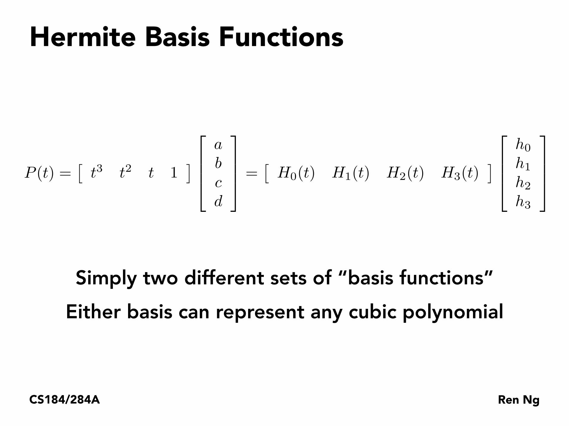
P (t) =[

t3 t2 t 1]

⎡

⎢

⎢

⎣

a

b

c

d

⎤

⎥

⎥

⎦

=[

H0(t) H1(t) H2(t) H3(t)]

⎡

⎢

⎢

⎣

h0

h1

h2

h3

⎤

⎥

⎥

⎦

Simply two different sets of “basis functions” Either basis can represent any cubic polynomial

Ren NgCS184/284A

Hermite Basis Functions

H0(t) = 2t3 � 3t2 + 1

H1(t) = �2t3 + 3t2

H2(t) = t3 � 2t2 + t

H3(t) = t3 � t2

H0(t) = 2t3 � 3t2 + 1

H1(t) = �2t3 + 3t2

H2(t) = t3 � 2t2 + t

H3(t) = t3 � t2

H0(t) = 2t3 � 3t2 + 1

H1(t) = �2t3 + 3t2

H2(t) = t3 � 2t2 + t

H3(t) = t3 � t2H0(t) = 2t3 � 3t2 + 1

H1(t) = �2t3 + 3t2

H2(t) = t3 � 2t2 + t

H3(t) = t3 � t2

H0(t) = 2t3 � 3t2 + 1

H1(t) = �2t3 + 3t2

H2(t) = t3 � 2t2 + t

H3(t) = t3 � t20

1

0

1

0

1

0

1

Ren NgCS184/284A

Ease Function

A very useful function In animation, start and stop gently (zero velocity)

H1(t) = �2t3 + 3t2 = t2(3� 2t)

H0(t) = 2t3 � 3t2 + 1

H1(t) = �2t3 + 3t2

H2(t) = t3 � 2t2 + t

H3(t) = t3 � t2

0

1

0

1

Ren NgCS184/284A

Hermite Spline Interpolation

Inputs: sequence of values and derivatives

Catmull-Rom Interpolation

Ren NgCS184/284A

Catmull-Rom Interpolation

Inputs: sequence of values

y0y1

y2

y3

0 1 2 3

Ren NgCS184/284A

Catmull-Rom Interpolation

Rule for derivatives: Match slope between previous and next values

1

2(y3 � y1)

0 1 2 3

1

2(y2 � y0)

Ren NgCS184/284A

Catmull-Rom Interpolation

Then use Hermite interpolation

0 1 2 31

2(y3 � y1)

1

2(y2 � y0)

y1

y2

Ren NgCS184/284A

Catmull-Rom Spline

Input: sequence of points

Output: spline that interpolates all points with C1 continuity

Interpolating Points & Vectors

Ren NgCS184/284A

Can Interpolate Points As Easily As Values

p3

p4 p0

p1

p2

Catmull-Rom 3D spline control points

E.g. point (0,1,3) in 3D space, or even a general vector in N dimensions

Ren NgCS184/284A

Can Interpolate Points As Easily As Values

p3

p4 p0

p1

p2

1

2(p2 � p0)1

2(p3 � p1)

1

2(p4 � p2)

Tangent Vectors

Catmull-Rom 3D tangent vectors

Ren NgCS184/284A

Can Interpolate Points As Easily As Values

p3

p4 p0

p1

p2

1

2(p2 � p0)1

2(p3 � p1)

1

2(p4 � p2)

Catmull-Rom 3D space curve

Use Basis Functions to Define Curves

General formula for aparticular interpolation scheme:

Coefficients pi can be points & vectors, not just values Fi(t) are basis functions for the interpolation scheme. Saw Hi(t) for Hermite interpolation earlier. Will see Ci(t) for Catmull-Rom shortly, and Bi(t) for Bézier scheme later. The basis functions are properties of the interpolation scheme.

p(t) =nX

i=0

piFi(t)

x(t) =nX

i=0

xiFi(t) y(t) =nX

i=0

yiFi(t) z(t) =nX

i=0

ziFi(t)

Ren NgCS184/284A

Matrix Form of Catmull-Rom Space Curve?

Use Hermite matrix form

• Points & tangents given by Catmull-Rom rules

P (t) =

2

664

t3

t2

t1

3

775

T 2

664

2 �2 1 1�3 3 �2 �10 0 1 01 0 0 0

3

775

2

664

0 1 0 00 0 1 0

� 12 0 1

2 00 � 1

2 0 12

3

775

2

664

p0

p1

p2

p3

3

775

Hermite points

Hermite tangents

h0 = p1

h1 = p2

h2 = 12 (p2 � p0)

h3 = 12 (p3 � p1)

Hermite matrix Convert Catmull-Rominputs to Hermite inputs

Ren NgCS184/284A

Matrix Form of Catmull-Rom Space Curve

Matrix columns = Catmull-Rom basis functions

P (t) =

2

664

t3

t2

t1

3

775

T 2

664

� 12

32

32

12

1 � 52 2 � 1

2� 1

2 0 12 0

0 1 0 0

3

775

2

664

p0

p1

p2

p3

3

775

= C0(t) p0 + C1(t) p1 + C2(t) p2 + C3(t) p3

Ren NgCS184/284A

Catmull-Rom Basis Functions

Bézier Curves

Ren NgCS184/284A

Examples of Geometry

Ren NgCS184/284A

Defining Cubic Bézier Curve With Tangents

p3

p0

p1

p2t0 = 3(p1 � p0)

t1 = 3(p3 � p2)

Ren NgCS184/284A

Matrix Form of Cubic Bézier Curve?

P (t) =

2

664

t3

t2

t1

3

775

T 2

664

⇥ ⇥ ⇥ ⇥⇥ ⇥ ⇥ ⇥⇥ ⇥ ⇥ ⇥⇥ ⇥ ⇥ ⇥

3

775

2

664

p0

p1

p2

p3

3

775

= B30(t) p0 +B3

1(t) p1 +B32(t) p2 +B3

3(t) p3

Good exercise to derive this matrix yourself.One way: use Hermite matrix equation again.

What are the points and tangents?

Demo – Piecewise Cubic Bézier Curve

David Eck, http://math.hws.edu/eck/cs424/notes2013/canvas/bezier.html

Evaluating Bézier Curves De Casteljau Algorithm

Ren NgCS184/284A

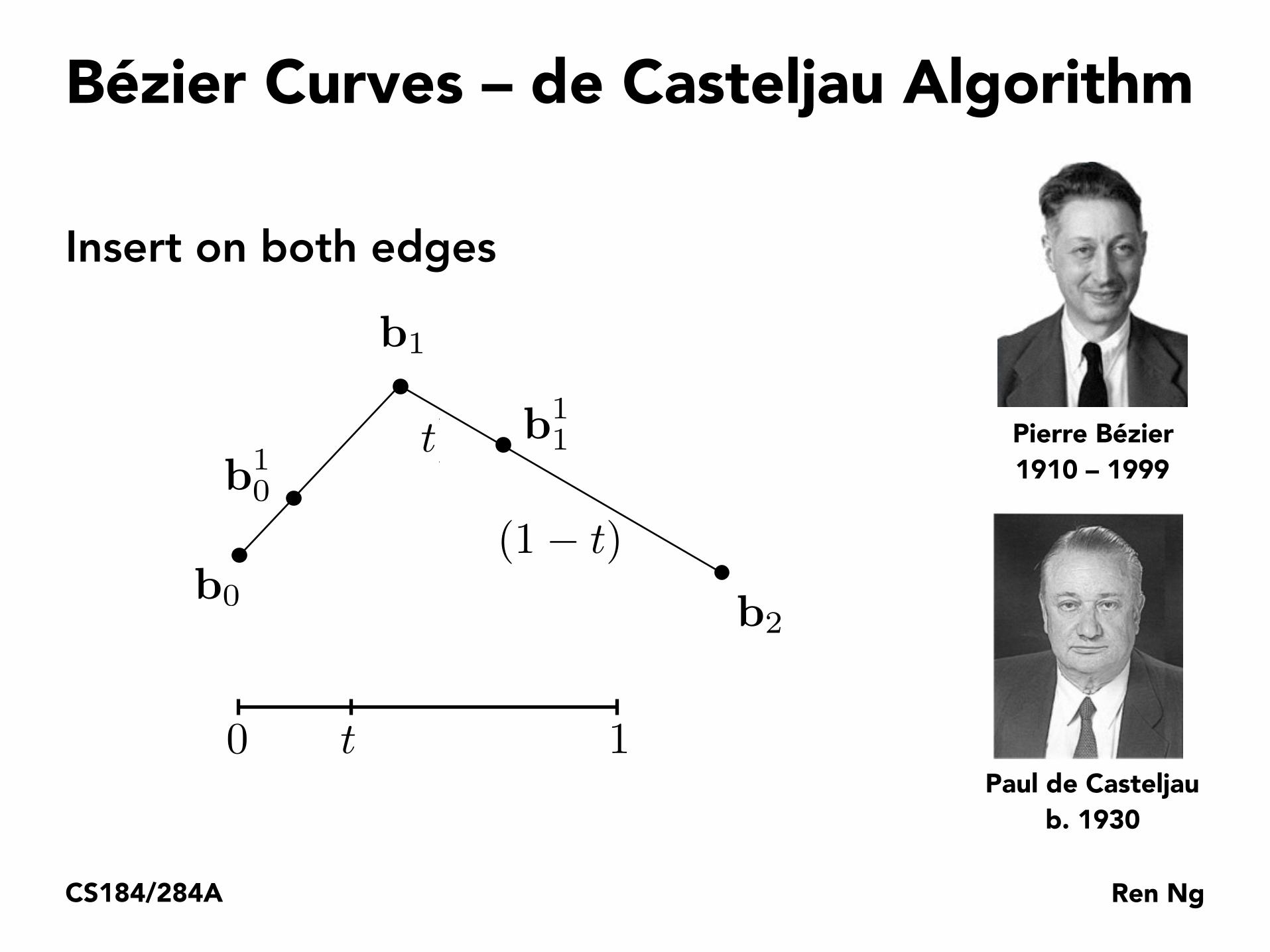
Bézier Curves – de Casteljau Algorithm

b0

b1

b2

Pierre Bézier 1910 – 1999

Paul de Casteljau b. 1930

Consider three points (quadratic Bezier)

Ren NgCS184/284A

Bézier Curves – de Casteljau Algorithm

b0

b1

b2

b1

0

0 1t

Pierre Bézier 1910 – 1999

Paul de Casteljau b. 1930

Insert a point using linear interpolation

(1� t)

(1� t)

Ren NgCS184/284A

Bézier Curves – de Casteljau Algorithm

b0

b1

b2

b1

0

b1

1

0 1t

Pierre Bézier 1910 – 1999

Paul de Casteljau b. 1930

Insert on both edges

(1� t)

(1� t)

Ren NgCS184/284A

Bézier Curves – de Casteljau Algorithm

b0

b1

b2

b1

0

b1

1b2

0

0 1t

Pierre Bézier 1910 – 1999

Paul de Casteljau b. 1930

Repeat recursively

(1� t)(1� t)

Ren NgCS184/284A

Bézier Curves – de Casteljau Algorithm

b0

b1

b2

b1

0

b1

1 Pierre Bézier 1910 – 1999

Paul de Casteljau b. 1930

Algorithm defines the curve

b2

0

“Corner cutting” recursive subdivision Successive linear interpolation

Visualizing de Casteljau Algorithm

Animation: Steven Wittens, Making Things with Maths, http://acko.net

Ren NgCS184/284A

Cubic Bézier Curve – de Casteljau

b00

b01

b02

b03

b10

b11

b12

b20

b21

x(t)

Consider four pointsSame recursive linear interpolations

b3

0

(1� t)

(1� t)

Ren NgCS184/284A

de Casteljau Algorithm Subdivides Curve

Control polygonfor full curve

Control polygonfor right curve

Control polygonfor left curve

b00

b01

b02

b03

b00

b10

b20

b3

0

b01

b02

b03

b11

b12

b21

b03

b12

b21b

3

0

b00

b01

b02

b10

b11

b20

Evaluating Bézier Curves Algebraic Formula

Ren NgCS184/284A

Bézier Curve – Algebraic Formula

de Casteljau algorithm gives a pyramid of coefficients

b00 b0

1 b02 b0

3

b10 b1

1 b12

b20 b2

1

b30 x(t)

(1� t) (1� t)

Ren NgCS184/284A

Bézier Curve – Algebraic Formula

b1

0(t) = (1 − t)b0 + tb1

b1

1(t) = (1 − t)b1 + tb2

b2

0(t) = (1 − t)b1

0 + tb1

1

b0

b1

b2

b1

0

b1

1

b2

0

0 1t

b20(t) = (1� t)2b0 + 2t(1� t)b1 + t2b2

Example: quadratic Bézier curve from three points

Ren NgCS184/284A

Bézier Curve – General Algebraic Formula

bn(t) = b

n0 (t) =

n∑

j=0

bjBnj (t)

Bn

i (t) =

(

n

i

)

ti(1 − t)n−i

Bernstein form of a Bézier curve of order n:

Bernstein polynomials:

Bézier control points

Ren NgCS184/284A

Cubic Bézier Basis Functions

Bn

i (t) =

(

n

i

)

ti(1 − t)n−i

Sergei N. Bernstein1880 – 1968

Bernstein polynomials:

B30(t)

B31(t) B3

2(t)

B33(t)

0

1

0

1

0

1

0

1

Piecewise Bézier Curves (Bézier Spline)

Ren NgCS184/284A

Higher-Order Bézier Curves?

High-degree Bernstein polynomials don’t interpolate well

Very hard to control! Uncommon

Piecewise Bézier Curves

Instead, chain many low-order Bézier curve Piecewise cubic Bézier the most common technique

Widely used (fonts, paths, Illustrator, Keynote, …)

Ren NgCS184/284A

Piecewise Bézier Curve – Continuity

Two Bézier curves a : [k, k + 1] ! IRN

b : [k + 1, k + 2] ! IRN

k k + 1 k + 2

Assuming integer partitions here, can generalize

Ren NgCS184/284A

Piecewise Bézier Curve – Continuity

C0 continuity: an = b0 =12

(an�1 + b1)

k k + 1 k + 2

Ren NgCS184/284A

Piecewise Bézier Curve – Continuity

1 : 1

C1 continuity: an = b0 =12

(an�1 + b1)

k k + 1 k + 2

Ren NgCS184/284A

Piecewise Bézier Curve – Continuity

1 : 11

: 1 1 : 1

C2 continuity: “A-frame” construction

di+1

k k + 1 k + 2

Ren NgCS184/284A

Properties of Bézier Curves

Interpolates endpoints

• For cubic Bézier: Tangent to end segments

• Cubic case: Affine transformation property

• Transform curve by transforming control points Convex hull property

• Curve is within convex hull of control points

b(0) = b0; b(1) = b3

b0(0) = 3(b1 � b0); b0(1) = 3(b3 � b2)

Bézier Surfaces

Ren NgCS184/284A

Bézier Surfaces

Extend Bézier curves to surfaces

Ed Catmull’s “Gumbo” model Utah Teapot

renderspirit.comP. Ri

deou

t

Ren NgCS184/284A

Bicubic Bézier Surface Patch

Bezier surface and 4 x 4 array of control points

Visualizing Bicubic Bézier Surface Patch

Animation: Steven Wittens, Making Things with Maths, http://acko.net

Ren NgCS184/284A

Visualizing Bicubic Bézier Surface Patch

4x4 control points

• Each 4x1 control points in u define a Bezier curve

• (4 Bezier curves in u)

• Corresponding points on these 4 Bezier curves define 4 control points for a “moving curve” in v

• This “moving” curve sweeps out the 2D surface

Evaluating Bézier Surfaces

Ren NgCS184/284A

Evaluating Surface Position For Parameters (u,v)

For bi-cubic Bezier surface patch, Input: 4x4 control points Output is 2D surface parameterized by (u,v) in [0,1]2

Ren NgCS184/284A

Method 1: Separable 1D de Casteljau Algorithm

Goal: Evaluate surface position corresponding to (u,v) (u,v)-separable application of de Casteljau algorithm

• Use de Casteljau to evaluate point u on each of the 4 Bezier curves in u. This gives 4 control points for the “moving” Bezier curve

• Use 1D de Casteljau to evaluate point v on the “moving” curve

Bezier curves in u

“Moving” Bezier curve

Surface point (u,v)

Ren NgCS184/284A

Method 1: Separable 1D de Casteljau Algorithm

Ren NgCS184/284A

Method 2: 2D de Casteljau Algorithm

Repeated application of bilinear interpolation

Ren NgCS184/284A

Method 2: 2D de Casteljau Algorithm

Example:

⎡

⎣

0

0

0

⎤

⎦

⎡

⎣

2

0

0

⎤

⎦

⎡

⎣

4

0

0

⎤

⎦

⎡

⎣

0

2

0

⎤

⎦

⎡

⎣

2

2

0

⎤

⎦

⎡

⎣

4

2

2

⎤

⎦

⎡

⎣

0

4

0

⎤

⎦

⎡

⎣

2

4

4

⎤

⎦

⎡

⎣

4

4

4

⎤

⎦

⎡

⎣

1

1

0

⎤

⎦

⎡

⎣

3

1

0.5

⎤

⎦

⎡

⎣

1

3

1

⎤

⎦

⎡

⎣

3

3

2.5

⎤

⎦

⎡

⎣

2

2

1

⎤

⎦

r = 1 r = 2 r = 3

(u, v) =

✓1

2,1

2

◆

Method 3: Algebraic Evaluation

Let the moving curve be a degree m Bézier curve

Let each control point bi be moving along a Bézier curve of degree n

Tensor product Bézier patch

bm(u) =

m∑

i=0

biBm

i (u)

bi = bi(v) =n∑

j=0

bi,jBnj (v)

bm,n(u, v) =

m∑

i=0

n∑

j=0

bi,jBmi (u)Bn

j (v)

(remember, Bernstein polynomials)B

n

i (t) =

(

n

i

)

ti(1 − t)n−i

Bézier Surface Continuity

Ren NgCS184/284A

Piecewise Bézier Surfaces

C0 continuity: Boundary curves

Ren NgCS184/284A

Piecewise Bézier Surfaces

C1 continuity: Collinearity

Ren NgCS184/284A

Piecewise Bézier Surfaces

C2 continuity: A-frames

Ren NgCS184/284A

Things to Remember

Splines

• Cubic Hermite and Catmull-Rom interpolation

• Matrix representation of cubic polynomials Bézier curves

• Easy-to-control spline

• Recursive linear interpolation – de Casteljau algorithm

• Properties of Bézier curves

• Piecewise Bézier curve – continuity types and how to achieve Bézier surfaces

• Bicubic Bézier patches – tensor product surface

• 2D de Casteljau algorithm

Ren NgCS184/284A

Acknowledgments

Thanks to Pat Hanrahan, Mark Pauly and Steve Marschner for presentation resources.