Bifurcation from codimension one relative homoclinic cycles Ale Jan Homburg KdV Institute for Mathematics, University of Amsterdam e-mail: [email protected]Alice C. Jukes Department of Mathematics, Imperial College London e-mail: [email protected]J¨ urgen Knobloch Department of Mathematics, TU Ilmenau e-mail: [email protected]Jeroen S.W. Lamb Department of Mathematics, Imperial College London e-mail: [email protected]July 23, 2007 Abstract We study bifurcations of relative homoclinic cycles in flows that are equivariant under the action of a finite group. The relative homoclinic cycles we consider are not robust, but have codimension one. We assume real principal eigenvalues and connecting orbits that approach the equilibria along principal directions. We show how suspensions of subshifts of finite type generically appear in the unfolding. Descriptions of the suspended subshifts in terms of the geometry and symmetry of the connecting orbits are provided. Contents 1 Introduction 2 2 Setting and main results 5 3 Lin’s method 12 3.1 Lin orbits .............................................. 13 3.2 Reference orbits ........................................... 16 3.3 Bifurcation equations ........................................ 18 4 Proof of the general bifurcation result 20 4.1 Solving the bifurcation equations ................................. 21 4.2 Topological conjugation ...................................... 22 5 Examples 25 5.1 Methodology ............................................ 25 5.2 Bifurcation with dihedral symmetry ............................... 26 5.2.1 One-dimensional E s p .................................... 27 5.2.2 Two-dimensional E s p . .................................... 30 Appendix 37 References 37 1
Transcript
Bifurcation from codimension one relative homoclinic cycles
Ale Jan HomburgKdV Institute for Mathematics, University of Amsterdam
We study bifurcations of relative homoclinic cycles in flows that are equivariantunder the action of a finite group. The relative homoclinic cycles we consider arenot robust, but have codimension one. We assume real principal eigenvalues andconnecting orbits that approach the equilibria along principal directions. We show howsuspensions of subshifts of finite type generically appear in the unfolding. Descriptionsof the suspended subshifts in terms of the geometry and symmetry of the connectingorbits are provided.
We study bifurcations from networks of heteroclinic connections between (heteroclinic net-works) in ordinary differential equations that are equivariant under the action of a finitegroup. Recall that heteroclinic connection between two equilibria is a solution that isbi-asymptotic (forwards and backwards in time) to these equilibria. When the asymptoticequilibrium at either end of the connection is the same, one usually calls the connectionhomoclinic. A heteroclinic cycle is a sequence of heteroclinic connections constituting adirected path from an equilibrium to itself. Heteroclinic cycles may give rise to nontrivialrecurrent dynamics. Heteroclinic cycles in equivariant flows can be of various codimensionand can in fact occur robustly. In this paper, we discuss the occurrence of heteroclinicnetworks of codimension one, i.e. networks which appear typically persistently in a oneparameter family of (equivariant) differential equations. We focus on generic codimensionone heteroclinic networks for which none of the constituting heteroclinic connections arerobust (i.e. of codimension zero), and show that such heteroclinic cycles are relative ho-moclinic cycles. A motivating example for our study is presented in [23] by Matthies ona Takens-Bogdanov bifurcation with D3-symmetry. This work contains a study of a rela-tive homoclinic cycle that fits into the theory developed in this paper. In the bifurcationscenario a D3-symmetric configuration of three Z2-invariant homoclinic orbits to the same(D3-invariant) equilibrium arises. In the unfolding Matthies found a suspended topolog-ical Markov chain. The bifurcations studied in [23] occur in systems for three coupledoscillators and for mode interactions in convection problems [11].
To motivate the setting of our bifurcation study, and to connect it to existing works onhomoclinic and heteroclinic cycles in equivariant flows, we start with some generalities.Given an ordinary differential equation, an orbit in the intersection of stable and unstablemanifolds of hyperbolic equilibria is called a heteroclinic orbit. For general differentialequations, stable and unstable manifolds of hyperbolic equilibria with the same index(dimension of the unstable manifold), will typically not intersect. Indeed, by the Kupka-Smale theorem [24] the set of Ck differential equations with such a heteroclinic connectionforms a set of Baire first category. Transversality arguments show that in one parameterfamilies of differential equations one can expect an intersection to occur persistently at aparameter value. An orbit in the intersection of the stable and unstable manifold of thesame equilibrium is called a homoclinic orbit. As this obviously is a connecting orbit be-tween equilibria of the same index, homoclinic orbits can be expected to occur persistentlyin one parameter families.
To make this more precise, consider a differential equation x = f(x) with x ∈ Rn. Given
two equilibria p− and p+ of it, a heteroclinic orbit {γ(t)}t∈R is a solution that convergesto p± as times goes to ±∞. Suppose p−, p+ are hyperbolic equilibria with indices ind(p−)and ind(p+). Heteroclinic orbits from p− to p+ can occur persistently only if p− haslarger index than p+. In fact, the set of heteroclinic connections forms a manifold ofdimension ind(p−)− ind(p+) if the unstable manifold of p− intersects the stable manifoldof p+ transversally. If the index of p− is smaller or equal to the index of p+, heteroclinicconnections from p− to p+ can only be found persistently (at isolated parameter values)in k-parameter families of differential equations for k = ind(p+)− ind(p−)+1. Needed is atransverse intersection of the stable and unstable manifolds of the equilibria in the productR
n × Rk of state space and parameter space. The number k is called the codimension of
the heteroclinic orbit.
The situation is markedly different for differential equations that possess a discrete sym-metry. The context we will assume in this paper is of a (parameter-dependent) differentialequation
x = f(x, λ), (1.1)
2
on Rn that is equivariant under the action of a finite group G (acting as diffeomorphisms
of Rn to itself): i.e.
x(t) is a solution of (1.1) ⇔ gx(t) is a solution of (1.1) ∀g ∈ G (1.2)
or in other words, if
Dg(u)f(u, λ) = f(u, λ)(g(u)), ∀g ∈ G. (1.3)
A solution x(t) is called symmetric with respect to a symmetry g ∈ G, if x(t) is setwiseinvariant under g. It follows that if a heteroclinic connection between two hyperbolicequilibria is symmetric with respect to a symmetry g ∈ G, then (since G is compact) itmust be pointwise invariant under g, and thus be entirely contained in its fixed pointsubspace Fix(g) := {u ∈ R
n | g(u) = u}. Within a fixed point subspace, equilibriacan have different indices even if they possess the same indices in R
n, thus altering thecodimension of the heteroclinic orbit. As a consequence, heteroclinic connections betweenequilibria of equal index may occur robustly in equivariant flows.
Heteroclinic networks are sets consisting of finitely many equilibria and finitely many het-eroclinic connections between them, such that each equilibrium can be reached from eachother equilibrium by a chain of connecting orbits. A heteroclinic network with hyperbolicequilibria has a codimension inherited from the codimensions of the heteroclinic orbits init. If the heteroclinic network is the image under the group action of a single heteroclinicorbit, it is also called a relative homoclinic cycle since on the quotient R
n/G such a hete-roclinic cycle is represented by a (single) homoclinic cycle. It follows that the codimensionof a relative homoclinic cycle is equal to that of its generating heteroclinic connection.
It was observed by dos Reis [6] and Field [7] that heteroclinic cycles can occur robustlyin equivariant flows. Guckenheimer and Holmes analyzed an explicit example [12]. Thegeometry that is often considered is where inside a fixed point space, there is a heteroclinicorbit from an equilibrium with one dimensional unstable manifold to an asymptoticallystable equilibrium. Such connections are clearly robust. Robust heteroclinic cycles canoccur more generally if, for each heteroclinic orbit in the heteroclinic cycle, the index ofthe α-limit point exceeds by one the index of the ω-limit point computed in the fixedpoint space of the isotropy group of the heteroclinic orbit. Indeed, if this is the case, theheteroclinic orbit can arise as a locally isolated transverse intersection of unstable andstable manifolds of equilibria. There has been a lot of interest in the existence, asymptoticstability and also bifurcations of robust heteroclinic cycles, see [3, 8, 20, 27] and referencestherein.
We study a class of bifurcations problems with codimension one relative homoclinic cycles.The most important restriction we will assume is the condition that the heteroclinic orbitsare tangent to the principal (leading) directions at the equilibria. Although this is thetypical case for general systems, it does not always hold for systems with symmetry.An important manifestation of symmetry is that it may enforce the linearisation at asymmetric equilibrium point to have multiple principal eigenvalues. Symmetry can alsoforce the simultaneous occurrence of several heteroclinic orbits, all related by symmetry.We show how Lin’s method, an analytic tool for the derivation of bifurcation equations forheteroclinic bifurcations [21, 25], can be applied to study the dynamics near codimensionone relative homoclinic cycles. While Lin’s method was developed for simple principaleigenvalues, we apply the techniques to heteroclinic bifurcations with multiple principaleigenvalues, using the fact that they arise in a semi-simple way.
The common picture in the bifurcations we encounter is the following. The relative homo-clinic cycle exists at an isolated parameter value. When breaking the relative homocliniccycle by varying the parameter, a recurrent set appears. The recurrent set, or at least
3
subsets of it, can be described through a conjugation with a topological Markov chain(or subshift of finite type, the reader can consult [16, 22] for generalities on topologi-cal Markov chains). The dynamics on both sides of the bifurcation value differ and aredescribed by different topological Markov chains. We explain the constructions of thetopological Markov chains which describe the changes in the recurrent set. There is anatural way to use symbolic dynamics in the description of the recurrent set, by using thelanguage of topological Markov chains mentioned above. Each heteroclinic connection isthereto assigned a symbol (e.g. a unique integer) and orbits near the homoclinic cycle areassigned a list of symbols describing near which connection the orbit traverses. In thiscontext, we recall the notion of the connectivity matrix C = [cij ] of a heteroclinic network,where cij = 1 if the endpoint (ω-limit) of heteroclinic connection j is equal to the startingpoint (α-limit) of heteroclinic connection i.
Below we state a general bifurcation theorem that makes this scenario more precise. Thecomplete constructions and conditions can be found in Section 2, where the main bifurca-tion theorem, Theorem 2.4 is formulated. A detailed account of possible homoclinic loopsand their bifurcations will be given for relative homoclinic cycles with dihedral symmetry,see Section 5, generalizing the D3-equivariant example considered by Matthies [23].
We introduce notation for topological Markov chains. Let
Bk = {1, . . . , k}Z (1.4)
denote the set of double infinite sequences κ : Z → {1, . . . , k}, i 7→ κi, equipped with theproduct topology. Let M = (mij)i,j∈{1,...,k} be a 0-1 matrix, that is mij ∈ {0, 1}. By Bk
M
we denote the topological Markov chain defined by M ,
BkM = {κ ∈ Bk : mκiκi+1
= 1}.
Let ζ be the left shift operating on Bk,
ζ : Bk → Bk, (ζκ)i = κi+1.
Observe that BkM
is ζ-invariant.
Theorem 1.1. Let x = f(x, λ) be a one parameter family of differential equations equiv-ariant with respect to a finite group G, with the following properties:
• At λ = 0, there is a relative homoclinic cycle H of codimension one.
• The connecting orbits in H approach the equilibria along the principal directions.
• The isotropy subgroup Gp := {g ∈ G | g(p) = p} of any equilibrium p ∈ H actsabsolutely irreducibly on the principal eigenspace at this equilibrium.1
Write γ1, . . . , γk for the connecting orbits that constitute H. There is an explicit construc-tion of k×k matrices M−, and M+ with coefficients in {0, 1} and the nonzero coefficientsin mutually disjoint positions, so that the following holds for any generic family unfoldinga homoclinic cycle as above.
Take cross sections Σi transverse to γi and write Πλ for the first return map on thecollection of cross sections ∪k
j=1Σj. For λ > 0 small enough, there is an invariant set
Dλ ⊂ ∪kj=1Σj for Πλ such that for each κ ∈ Bk
M+there exists a unique x ∈ Dλ with
1Note that by Bochner’s Theorem [1], the action of the isotropy subgroup can be taken to be linearwithout loss of generality. Recall that a (real) linear representation is called absolutely irreducible if theset of linear maps commuting with this representation is isomorphic to R [10].
4
Πiλ(x) ∈ Σκi. Moreover, (Dλ,Πλ) is topologically conjugated to (Bk
M+, ζ). An analogous
statement holds for λ < 0 with BkM+
replaced by BkM−
.
This above description of the dynamics provides a complete picture of the local nonwan-dering dynamics near H if and only if
M+ + M− = C, (1.5)
where C denotes the connectivity matrix of the relative homoclinic network.
It should be noted that (1.5) is often, but not always satisfied. In the latter case, thetopological Markov chain described above describes part of the recurrent set. It is how-ever possible to describe the situations where we need to confine ourselves to describinginvariant subsets of the recurrent set. Here we just comment that depending on the groupand its representations on leading eigenspaces, the obstructions are either always avoided,or generically avoided, or enforced. We finally note that we do not prove the hyperbolicityof the recurrent sets as the functional analytic methodology does not (yet) provide toolsfor proving this (but we are confident of hyperbolicity if the condition (1.5) is satisfied).
This paper is organized as follows. In the next section we start with the standing assump-tions for our study and formulate our main results. A more technical section, Section 3,follows in which the techniques developed by Lin [21] and Sandstede [25] to derive bi-furcation equations for orbits in the recurrent set are adapted to the present context.In Section 4 these techniques are applied to prove the main theorem, Theorem 2.4. Acatalogue of bifurcation scenarios for relative homoclinic cycles in systems with dihedralsymmetry is derived in Section 5. In order to illustrate a mechanism by which (1.5) can beviolated, in the appendix we describe some aspects of examples with tetrahedral symmetry.
2 Setting and main results
In this section we fix the class of systems under consideration, introduce conditions on theaction of the symmetry and the geometry of the flow, and present the general bifurcationtheorem Theorem 2.4.
Consider a one-parameter family of vector fields f : Rn × R → R
n, f smooth,
x = f(x, λ). (2.1)
Throughout the paper we assume that f is equivariant with respect to a smooth groupaction of a finite group G, i.e. there is a mapping ρ (the action of the group, see [2])
ρ : G → Diff(Rn).
Saying that ρ is an action means that it is a homomorphism. In the neighbourhoodof an equilibrium point p with istropy Gp, by Bochner’s Theorem we may choose localcoordinates such that ρ : Gp → O(n) where O(n) denotes the group of linear orthogonaltransformations from R
n to itself. The latter action is usually called a representation.A representation is faithful if the homomorphism is injective, it is trivial if each groupelement acts as the identity. Equivariance of f means that (1.2) and (equivalently) (1.3)hold.
We aim to study codimension one heteroclinic networks, which contain no robust hetero-clinic connections. Such a heteroclinic network should be generated by a single connectingorbit between hyperbolic equilibria, where the equilibria lie in a single group orbit. If thiscondition is not met, it is easy to see that the codimension of the network must be at
5
least two, as there would be at least two completely independent heteroclinic connectionswhich each have codimension at least one. Note that the equilibria can be equal, in whichcase a collection of homoclinic loops will be obtained.
In more detail the construction is as follows. At λ = 0 there are hyperbolic equilibria pand hp for some h ∈ G, and an orbit γ(·) connecting p to hp. Thus limt→−∞ γ(t) = p andlimt→∞ γ(t) = hp. In general, given a connecting orbit γ(·) between two equilibria, wewrite α(γ) and ω(γ) for the α and ω limits of points on γ:
α(γ) = limt→−∞
γ(t) ω(γ) = limt→∞
γ(t).
WriteΓ = {γ(t), t ∈ R}.
Due to the equivariance of the vector field any g-image g(O) of an orbit O is again anorbit. Let
H = G(Γ ∪ {p})
be the group orbit of the closure of Γ. The above implies that G acts transitively on theset of equilibria in H. As a consequence, the spectrum is the same at all equilibria.
Recall that the isotropy group Gq of a point q is defined by
Gq = {g ∈ G | gq = q}.
Note that each point of an orbit has the same isotropy subgroup, so it makes sense tospeak of the isotropy subgroup GΓ of Γ.
For efficiency of the description, it is natural to focus on the case that H is connected.Namely, if it were not connected, there would be several connected components, each ofwhich is invariant under the action of a subgroup of G, so that each of these componentscan be studied individually as being equivariant with respect to this subgroup, withoutloss. In this context, we note the following lemma.
Lemma 2.1. Let group G act transitively on a symmetric network that is generated bythe closure of one connection from p to hp. Then the network is connected if and only if
G = 〈h,Gp〉.
Proof. Label the equilibria according to which element of G takes p to each one. First weshow that
G = 〈S〉
whereS = {g ∈ G| there is a heteroclinic connection from p to gp}.
Define subset
C :=
{
g ∈ G p is connected to gp via a path in the network,respecting the direction of the flow
}
.
First we show that 〈S〉 ⊂ C. Clearly S ⊂ C because S is just the nearest neighbours of p.We show that C is a subgroup, hence contains all of 〈S〉.If g ∈ C with gk ∈ Gp then Γ and gΓ form a path from p to g2p, Γ∪gp∪gΓ∪g2p∪ ...gk−1Γform a path from p to gk−1p. If gk ∈ Gp then g−k ∈ Gp since Gp is a subgroup. Nowg−1p = gk−1g−kp = gk−1p since g−k ∈ Gp. Thus there is a path from p to g−1p andg−1 ∈ C.If g1, g2 ∈ C then there are paths from p to g1p and to g2p. Thus there is a path from g1p
6
to g1g2p which is the image under g1 of the path from p to g2p. Concatenating these givesa path from p to g1g2p. Hence g1g2 ∈ C. Thus C is subgroup of G.
Now we show that C ⊂ 〈S〉, that is, the connected network is only that generated by S.Suppose g ∈ C. Then because G is transitive there is a path in the network from p togp via g1p, ..., glp. Thus g1 ∈ S. We have a path g1p to g2p so there is a path from p tog−11 g2p so g−1
1 g2 ∈ S. Now since 〈S〉 is closed g2 = g1(g−11 g2) ∈ 〈S〉. By induction in this
way, g ∈ 〈S〉.
Now we show that 〈S〉 = 〈h,Gp〉.By definition h ∈ S. The images of the connection from p to hp under elements of Gp areconnections from p because they all fix p. Hence Gp ⊂ 〈S〉. Thus 〈h,Gp〉 ⊂ 〈S〉.Since the network is generated by a single connection all the connections that tend to pas t → −∞ are images of the connection from p to hp. Given g ∈ S the connection fromp to gp is gΓ for some g ∈ G. Since the connection is from p, g ∈ Gp. Thus gp = ghp. Butgh ∈ 〈h,Gp〉 so g ∈ 〈h,Gp〉. Hence S ⊂ 〈h,Gp〉.
To summarize the above, we assume the following to hold:
(H 1) H is a connected relative homoclinic cycle.
As formulated by the following hypothesis, inside
PΓ = FixGΓ = {x ∈ Rn | gx = x, g ∈ GΓ}
the connection is assumed to be of codimension one. Note that Γ ⊂ PΓ. Write indPΓ(p)
for the index dim(W u(p) ∩ PΓ) of p inside PΓ.
(H 2) indPΓ(p) = indPΓ
(hp).
Note that if indPΓ(p) > indPΓ
(hp), then W u(p) and W s(hp) can intersect transversallyinside PΓ. This brings the existence of heteroclinic solutions between p and hp in a robustway. The set of heteroclinic connections between p and hp is then a manifold of dimensionindPΓ
(p) − indPΓ(hp). If this number equals one, a locally isolated heteroclinic solution γ
from p to hp occurs in a robust way. This condition is in particular fullfilled if hp is anasymptotically stable equilibrium inside PΓ, an assumption appearing in the context ofasymptotically stable heteroclinic cycles.
The principal eigenvalues at a hyperbolic equilibrium are those nearest to the imaginaryaxis, either with positive or negative real parts. Principal stable eigenvalues are theprincipal eigenvalues with negative real part, principal unstable eigenvalues have positivereal part. Denote by µs(λ) and µu(λ) the principal stable and unstable eigenvalues ofD1f(hp, λ) and D1f(p, λ), respectively, assuming without loss that p and hp are equilibriafor all λ. By the smoothness of the vector field, µs(λ) and µu(λ) depend smoothly onλ. For conciseness write µs = µs(0) and µu = µu(0). By Es
hp and Eup we denote the
eigenspaces of the principal eigenvalues µs and µu.
Recall that the linear action of a group on a real vector space V is absolutely irreducible ifthe only linear maps with which the action of group elements commutes, are multiplicationsby constants. In the codimension one bifurcation problem at hand, it is readily verifiedthat the action of G on Es
hp and Eup is typically irreducible or the direct sum of two
As a nonresonance condition, we assume that (by changing the direction of time, if neces-sary)
7
(H 3) The isotropy subgroup Ghp acts absolutely irreducibly on Eshp (so that µs ∈ R)
and |µs| < Re(µu).
We note that equivariance never implies violation of this condition, but if the absolutelyirreducible representation has dimension m, then consequently µs has multiplicity m (andis semi-simple).
As we will see in Lemma 3.3, the limit
eshp = limt→∞
γ(t)/‖γ(t)‖
exists. This vector is assumed to lie in the principal direction:
(H 4) eshp ∈ Eshp
We note that the isotropy subgroup of Γ is a subgroup of the isotropy group of eshp:
GΓ ⊂ Geshp
. Consequently, we have eshp ∈ PΓ.
The demand that eshp lies inside the principal direction leaves out an interesting class
of codimension one relative homoclinic cycles where the symmetry (to be precise, therepresentations on leading eigenspaces) forces the connections to approach the equilibriaalong non-principal directions. In Section 5 an example is given (Case 4) where thissituation arises for a heteroclinic network with Dm-symmetry with m ≥ 3 odd.
In order to avoid a geometric configuration of manifolds similar to that arising at aninclination flip in systems without symmetry [13], we require that
(H 5) PΓ ∩Esp 6= {0}
Again, we need to emphasize that there exist certain equivariant codimension one bifur-cations where (H 5) is not satisfied, an example is given in the Appendix. An analysis ofthese bifurcations is beyond the scope of this paper.
We further assume that the heteroclinic orbit γ is nondegenerate:
(H 6) The tangent spaces of the unstable manifold W u(p) of p and of the stablemanifold W s(hp) of hp intersect in Γ only along the vector field direction.
We note that we use this hypothesis in our analysis, but we cannot exclude that thereexist situations where equivariance forces this hypothesis to fail.
The remaining condition we formulate implies that Γ is a codimension-one connectingorbit, unfolding generically with the parameter λ. The condition contains the familiarnondegeneracy condition for general flows to avoid inclination flip inside the flow invariantfixed point space PΓ.
A local center unstable manifold W cu(p) of p is a locally invariant manifold with as tangentspace at p the direct sum of the unstable and the principal stable directions. Likewise, alocal center stable manifold W cs(hp) of hp is a locally invariant manifold with as tangentspace at hp the direct sum of the stable and the principal unstable directions. Localcenter (un)stable manifolds are not unique, but possess unique tangent spaces along the(un)stable manifold.
See [13] for further generalities on invariant manifolds and foliations near equilibria.
The following hypothesis concerns the vector field x = f(x, λ) restricted to PΓ, which is aflow-invariant subspace. Denote by F ss
x the strong stable fibers inside the stable manifoldof hp and let F ss = ∪x∈ΓF
ssx . Let the subscript PΓ denote a restriction to PΓ.
8
(H 7) F ssPΓ
, and W cuPΓ
(p) intersect transversally along Γ (in PΓ):
F ssPΓ
tΓ WcuPΓ
(p). (2.2)
The bifurcation unfolds generically
W uPΓ
(p),W sPΓ
(hp) split with positive speed in λ. (2.3)
The transversality expressed by (2.2) implies that a tangent space F ssx plus a tangent
space TxWcu(p) spans a subspace of maximal dimension.
Condition (H 3) implies a nonresonance condition for the flow restricted to PΓ. See [4] forhomoclinic bifurcation problems in generic systems with resonant eigenvalues. Condition(H 4) excludes an orbit flip condition, see [25], while (2.2) is a generalization of the non-inclination flip condition, see [15, 17]. Note these conditions are automatically satisfied ifPΓ is two dimensional, independent of the dimension of the entire space.
Lemma 2.2. Suppose Hypotheses (H 1) – (H6) are met. Then by an arbitrary smallperturbation of the differential equation, Hypothesis (H 7) will be met, and inside PΓ,
TFss is a continuous vector bundle along Γ ∪ {p, hp}. (2.4)
Proof. Initially, we require only a small perturbation of the vector field restricted to PΓ
the existence of which follows from the general theory without symmetry [13]. Thoseperturbations can be extended to a small equivariant perturbation of f in the phase spacein the neighbourhood of PΓ. Note that by averaging over the group a small perturbationf can be made equivariant:
1
|G|
∑
g∈G
gfg−1
is equivariant. The first part of the lemma thus follows.
Statement (2.4) is a variant of the strong λ-lemma as found in [5].
As the statement is for λ = 0, we will write f(x) = f(x, 0). Denote by ϕt the flow of f .Then Dϕt(x) is the flow of the variational equation along {ϕt(x)}. Let Gss(R
n) be theGrassmannian manifold of linear subspaces in R
n with dimension dimEss. Lift f to aninduced vector field f on R
n × Gss(Rn), by defining its flow:
ϕt(x, α) = (ϕt(x), Dϕt(x)α).
Observe that this is a skew product flow. Clearly, (p,Ess) is an equilibrium of f . A directcomputation shows that (p,Ess) is a hyperbolic equilibrium and the unstable directionsinclude the tangent space of the fiber {p} × TEssGss(R
n), see e.g. [13].
Consider Fssq at a point q near p. As F ss
q is transversal to W cu(p), TqFssq is close to Ess by
standard cone field constructions, see e.g. [16]. The orbit of (q, TqFssq ) under the flow of
f lies therefore in the unstable manifold of (p,Ess). This implies continuity of the bundleTxF
ssx , x ∈ Γ. Continuity of TxF
uux , x ∈ Γ, is similar.
Our goal is to describe the recurrent set near H for parameter values of λ near 0. Considerthat H consists of finitely many, namely |G|/|GΓ|, connecting orbits. Here |H| denotes thecardinal number of the group H. The connecting orbits that make up H are denoted byγ1, . . . , γk. Likewise, write Γ1, . . . ,Γk. We can choose the time parameterization of theconnecting orbits so that for each i ∈ {1, . . . , k} there is a gi ∈ G with γi(·) = giγ(·).
9
Because G is compact we may assume that a G-invariant 〈·, ·〉 inner product is given. Wemay choose 〈·, ·〉 so that TpW
s(p) ⊥ TpWu(p) for an equilibrium p in H and therefore by
Hypothesis (H 1) for each equilibrium in H. Let, with respect to the G-invariant innerproduct 〈·, ·〉,
Yi = {f(γi(0), 0)}⊥, i ∈ 1, . . . , k.
ThenΣi = γi(0) + Yi, i ∈ 1, . . . , k (2.5)
is a hyperplane intersecting Γi transversally at γi(0). Due to the G-invariance of the innerproduct 〈·, ·〉, we have G(Σ1) = {Σi|i = 1, . . . , k}. Let
Zi =(
Tγi(0)Ws(ω(γi)) + Tγi(0)W
u(α(γi))⊥
(2.6)
be the subspace of Yi perpendicular to the tangent spaces at γ(0) of the stable and unstablemanifolds whose intersection defines γi. Note that the subspaces Zi, i = 1, . . . , k, are g-images of each other. Further, γi(0) + Zi ⊂ Σi. As a consequence of Hypothesis (H 6),dimZ1 = 1, and using that all equilibria are related by symmetry,
dimZi = 1
for all i. We can thus take a unit vector ψ1 ∈ Z1 spanning Z1. Take further vectorsψi ∈ Zi belonging to the G-orbit of ψ1 ∈ Z1. Due to the invariance of the inner productall ψi have norm 1.
Lemma 2.3. For each λ close to 0 there are unique pairs (γ+i (λ)(·), γ−i (λ)(·)) of orbits of
(2.1) such that
(i) γ±i (·)(0) smooth and γ±i (0)(0) = γi(0),
(ii) γ+i (λ)(0) ∈ Σi ∩W
s(ω(γi), λ), γ−i (λ)(0) ∈ Σi ∩Wu(α(γi), λ),
(iii) |γ+i (λ)(t) − γi(t)| small ∀t ∈ R
+ and |γ−i (λ)(t) − γi(t)| small ∀t ∈ R−,
(iv) γ+i (λ)(0) − γ−i (λ)(0) ∈ Zi.
Proof. The statements are a direct consequence of transversality of the intersection of∪x∈W s(ω(γi),λ) (x+ Zi) with W u(α(γi)) inside Σi near γi(0). That the intersection istransversal follows from Hypothesis (H 6). Observe that the intersection is a single point,which we denote γ−i (λ)(0). The point γ+
i (λ)(0) is given as(
γ−i (λ)(0) + Zi
)
∩W s(ω(γi), λ).
In [19, 25] integral expressions are derived for the difference γ+i (λ)(0) − γ−i (λ)(0).
Recall from the introduction that, for a given 0-1 matrix M , BkM
is the topological Markovchain defined by M . For κ ∈ Bk
M, we denote an orbit of (2.1) by x(λ, κ)(·) if there is a
monotonically increasing sequence (τi)i∈Z such that
x(λ, κ)(τi) ∈ Σκi , x(λ, κ)(t) 6∈k∪
j=1Σj, if t 6∈ {τi, i ∈ Z}.
We call κ the itinerary of x(λ, κ)(·). Let Πλ be the first return map defined on ∪kj=1Σj (in
fact the domain of Πλ is only a subset of ∪kj=1Σj):
Πλ : ∪kj=1Σj → ∪k
j=1Σj , Πλ(x(λ, κ)(τi)) = x(λ, κ)(τi+1). (2.7)
10
The main result below describes the way recurrent sets change through the bifurcation.The following definitions serve to define the topological Markov chains to which the firstreturn map on (subsets of) the recurrent set is conjugate. Define
esi = limt→∞
γi(t)/‖γi(t)‖.
To elucidate the symmetrical relation with definitions of further vectors e−j below, weprovide an equivalent definition via the variational equation. Let ζi(t) = γi(t) be thesolution to
v(t) = D1f(γi(t), 0)v(t), v(0) = −γi(0).
Thenesi = lim
t→∞ζi(t)/‖ζi(t)‖.
By Hypothesis (H 7) (more precisely, (2.3)), one can take w0 ∈ Zi so that
∂/∂λ〈γ+i (λ)(0) − γ−i (λ)(0), w0〉 > 0. (2.8)
That is, w0 is chosen such that the splitting of stable and unstable manifolds is in thedirection of w0. Let ζj(t) be the solution to the adjoint variational equation
w(t) = −D1f(γj(t), 0)∗w(t), w(0) = w0.
The initial condition guarantees that ζj(t) converges to 0 as t→ ±∞, see Section 3. Define
e−j = limt→−∞
ζj(t)/‖ζj(t)‖.
The existence of the limit is guaranteed by Lemma 3.4. The vector e−j is contained in
the principal unstable space E− of D1f(α(γj))∗, which equals Es by the choice of inner
product.
Given a matrix A , write |A | = (|aij |).
Theorem 2.4. Assume Hypotheses (H 1), (H 2), (H 4), (H 6), (H 7). Define the matrixA = (aij)i,j∈{1,...,k} by
aij =
{
0, if ω(γi) 6= α(γj),sgn 〈esi , e
−j 〉, if ω(γi) = α(γj).
WriteM+ = 1/2(A + |A |), M− = −1/2(A − |A |).
For λ > 0 small enough, there is an invariant set Dλ ⊂ ∪kj=1Σj for Πλ such that for each
κ ∈ BkM+
there exists a unique orbit x(·, λ, κ) with x(0, λ, κ) ∈ Dλ. Moreover, (Dλ,Πλ) is
topologically conjugated to (BkM+
, ζ).
An analogous statement holds for λ < 0 with BkM+
replaced by BkM−
.
If the inner products 〈esi , e
−j 〉 are different from 0 for all i, j with ω(γi) = α(γj), then the
recurrent set of f(·, 0) is the homoclinic cycle H. In this case the above described recurrentorbits for λ > 0 and λ < 0 provide the entire recurrent set.
Applied to a single symmetric homoclinic orbit, Theorem 2.4 gives the symmetric equiva-lent to the usual blue sky catastrophe [26].
Corollary 2.5. Assume in addition to Hypotheses (H 1), (H 2), (H 4), (H 6), (H 7), thatγ is a symmetric homoclinic orbit to a symmetric equilibrium p: GΓ = Gp = G. Then fhas a periodic solution for λ on one side of 0. The periodic orbit converges as a set to Γwhen λ→ 0 while developing infinite period and disappears in λ = 0.
11
Proof. We get A = (±1).
Remark 2.6. The structure of A depends on the isotropy group of Γ and the G-actionon Es (the eigenvalue condition in hypothesis (H 3) is the relevant factor for the absenceof the G-action on Eu). Every column and every row in A contains the same number ofequal coefficients 0,−1 or 1.
Remark 2.7. An occurrence of vanishing inner products in A forces us to describe onlysubsets of the recurrent set. A full treatment in his case would require the derivation ofhigher order terms in the bifurcation equations. Worked out examples in Section 5 willshow that depending on the group and its representation, vanishing inner products in thedefinition of A are either always avoided, or generically avoided, or enforced.
We say that a state X is accessible from a state Y , if the chain admits a finite directedpath from Y to X. Following [22], we consider an equivalence relation between states ofa Markov chain: X ∼ Y if X is accessible from Y and vice-versa. A Markov chain is saidto be reducible if the number of equivalence classes is greater than one. The transitionmatrices M± may define reducible topological Markov chains. For instance, (Bk
M±, ζ) may
allow only finitely many (periodic) orbits, e.g. if M± equals the identity matrix.
An equivalence class is called closed if every state is accessible only from within its ownequivalence class. Because of symmetry (since G is finite and acts transitively on theheteroclinic connections), it follows that the Markov chains defined by M± only admitclosed equivalence classes.
Examples studied in Section 5 provide several examples of the matrix A . Dynamics nearhomoclinic cycles in systems that are equivariant with respect to an action of a dihedralgroups G = Dm are classified in Section 5.
We finally note that our results, although formulated and proved in Rn, also apply to
dynamical systems on a smooth manifold M. Namely, by Whitney’s embedding theorem,if dimM = m, M can be embedded in R
2m. One may consider a (parameter dependent)dynamical system in R
2m with invariant submanifold M, in such a way that M is anormally hyperbolic invariant manifold (for all parameter values of interest). In this way,the analysis presented in this paper for vector fields in R
n also covers the analysis ofhomoclinic bifurcations on general smooth finite dimensional manifolds.
3 Lin’s method
The following concept for analyzing the dynamics near a heteroclinic chain is due to Lin[21]; the ideas for estimating the jumps have been introduced by Sandstede [25]. See also[19] for a presentation of Lin’s method.
In our presentation we restrict to chains which are related to the bifurcation problem statedin Section 2. Recall that heteroclinic orbits γ1, . . . , γk are given. Let κ ∈ Bk, where Bk isthe set if double infinite sequences on k symbols (see (1.4)), be fixed. A heteroclinic chainΓκ is a double infinite sequence of connecting orbits γκi , i ∈ Z, so that ω(γκi−1
) = α(γκi).Write
pκi = ω(γκi−1) = α(γκi).
Thus for each fixed index i ∈ Z, Γκi lies in the intersection of the unstable manifoldW u(pκi) of pκi and the stable manifold W s(pκi+1
) of pκi+1.
12
3.1 Lin orbits
Recall that Σi is a cross section transverse to Γi and the subspace Zi gives the directionperpendicular to the stable and unstable manifolds W s(ω(γi)), W
u(α(γi)) at γi(0), see(2.5), (2.6). Given a sequence ω = (ωi)i∈Z of sufficiently large transition times ωi > 0one can prove the existence of a unique piecewise continuous orbit x = (xi)i∈Z with thefollowing properties:
1. Each xi is an orbit of the vector field, starting at a point on Σκi−1, staying close to
Γκi−1until it reaches a neighborhood of pκi , and then continuing close to Γκi until it
reaches Σκi at time 2ωi,
2. The jump Ξi, defined as the difference between the initial point of xi+1 and the finalpoint of xi, belongs to the subspace Zκi .
Figure 1 visualizes the orbits with jumps in the cross sections. In what follows we willrefer to such orbits with jumps as Lin orbits.
γκi−1
ΣκiΣκi−1
xi+1
Ξκi
γκi
pκipκi+1
γκi(0)
γκi(0) + Zκi
x+i−1 x−
i
xi
Figure 1: Lin’s method involves the construction of piecewise continuous orbits followinga heteroclinic chain with jumps in a fixed direction at points in cross sections.
Allowing the vector field to depend on a parameter λ we have both the Lin orbit x andthe corresponding jump Ξ = (Ξi)i∈Z depending on ω, λ and κ ∈ Bk:
x = x(ω, λ, κ), Ξ = Ξ(ω, λ, κ).
In order to obtain an actual orbit which stays for all time close to the heteroclinic chainΓκ one has to set the jumps equal to zero, yielding the bifurcation equation
Ξ(ω, λ, κ) = 0.
The single jumps take the form
Ξi(ω, λ, κ) = ξ∞κi(λ) + ξi(ω, λ, κ),
where ξ∞κi(λ) measures the splitting of the stable and unstable manifolds of pκi+1
and pκi ,respectively. The expression ξi(ω, λ) is shown to be exponentially small as ω tends toinfinity; also explicit expressions are obtained for the leading terms of ξi(ω, λ).
In [19, 25] the estimates of the leading terms of ξi are derived for simple leading eigenvaluesµs and µu. In the present paper principal eigenvalues are in general semi-simple. Althoughthe estimates here can be attained in the same way as for simple principal eigenvalues, we
13
will present the main steps in their derivation. For that purpose we must in some detailtreat the construction of Lin orbits.
Actually xi+1(·) will be composed of orbits x+i (·) and x−i+1(·) which are defined on [0, ωi+1]
and [−ωi+1, 0], respectively. This demands coupling conditions
x+i (ωi+1) = x−i+1(−ωi+1), (3.1)
and jump conditionsΞi = x+
i (0) − x−i (0) ∈ Zκi , (3.2)
for i ∈ Z. We look for solutions of the form
x±i (t) = γ±κi(t) + v±i (t), (3.3)
where γ±κiare given by Lemma 2.3.
The following proposition ensures the existence of Lin orbits for each given sequence oftransition times.
Proposition 3.1. Let κ ∈ Bk be fixed. For each sequence ω = (ωi)i∈Z and each λ thereare unique functions v±i (ω, λ, κ)(·) such that x±i (defined in accordance with (3.3)) satisfyboth the coupling condition (3.1) and jump condition (3.2).
Proof. We give merely an outline of the arguments, providing some statements for lateruse. Detailed proofs can be found in [18, 25, 29].
First we define appropriate direct sum decompositions and projections. Assigned to γj(0),j ∈ {1, . . . , k}, consider the following orthogonal direct sum decompositions of R
n:
Rn = span {f(γj(0), 0)} ⊕W+
j ⊕W−j ⊕ Zj , (3.4)
where W+j = Tγj(0)W
s(ω(γj)) ∩ Yj and W−j = Tγj(0)W
u(α(γj)) ∩ Yj . Consider the varia-tional equations
v = D1f(γ±j (λ)(t), λ)v,
defined on R±, and corresponding transition matrices Φ±
j (λ, ·, ·). One can define projec-
tions P±j satisfying
kerP+j (λ, 0) = Tγ+
j (λ)(0)Ws(ω(γj)), imP+
j (λ, 0) = W−j ⊕ Z,
kerP−j (λ, 0) = Tγ−
j (λ)(0)Wu(α(γj)), imP−
j (λ, 0) = W+j ⊕ Z,
that are commuting with Φ±j (λ, ·, ·),
P±j (λ, t)Φ±
j (λ, t, s) = Φ±j (λ, t, s)P±
j (λ, s).
These projections are related to the exponential dichotomies of the variational equations.In the limit t→ ±∞, P±
j (λ, t) converge to projections onto stable and unstable subspacesat the equilibria,
limt→∞
kerP+j (λ, t) = Tω(γ+
j )Ws(ω(γj)), lim
t→∞imP+
j (λ, t) = Tω(γ+
j )Wu(ω(γj)),
limt→−∞
kerP−j (λ, t) = Tα(γ−
j )Wu(α(γj)), lim
t→−∞imP−
j (λ, t) = Tα(γ−
j )Ws(α(γj)).
(3.5)
For a given sequence of transition times ω we denote by Vω the space of all sequencesv = ((v+
i , v−i ))i∈Z with (v+
i , v−i ) ∈ C[0, ωi+1] ×C[−ωi, 0]. Endowed with the norm ‖v‖ :=
max{supi∈Z ‖v+i ‖, supi∈Z ‖v−i ‖}, Vω is a Banach space.
14
The v±i introduced in (3.3) solve the (nonlinear) variational equation along γ±κi:
v±i = D1f(γ±κi(λ)(t), λ)v±i + h±κi
(t, v±i (t), λ), (3.6)
where
h±κi(t, v, λ) = f(γ±κi
(λ)(t) + v, λ) − f(γ±κi(λ)(t), λ) −D1f(γ±κi
(λ)(t), λ)v.
Here v±i must satisfy certain boundary conditions stipulated by coupling and jump con-ditions on x±i :
v+i (ωi+1) − v−i+1(−ωi+1) = γ−κi+1
(λ)(−ωi+1) − γ+κi
(λ)(ωi+1) =: di+1(ω, λ, κ), (3.7)
v+i (0) − v−i (0) ∈ Zκi . (3.8)
Write d(ω, λ, κ) = (di(ω, λ, κ))i∈Z.
In order to solve the boundary value problem (3.6)–(3.8) we perform several steps. Firstwe “linearize” Equation (3.6) by replacing h+
κiand h−κi
by some g+i ∈ C[0, ωi+1] and
g−i ∈ C[−ωi, 0], respectively:
v±i = D1f(γ±κi(λ)(t), λ)v±i + g±i (t, λ). (3.9)
Simultaneously we replace the boundary condition (3.7) by prescribing projections a+i and
a−i of v+i−1(ωi) and v−i (−ωi):
a+i = (id− P+
κi−1(λ, ωi))v
+i−1(ωi), a−i = (id − P−
κi(λ,−ωi))v
−i (−ωi). (3.10)
The corresponding sequences we denote by g = (g+i , g
−i )i∈Z and a = (a+
i , a−i )i∈Z. The
variational equation (3.9) with boundary conditions (3.8), (3.10) has a unique solutionv(ω, λ,g,a, κ) = (v+
i , v−i )i∈Z. We remark that the quantities v±i do not depend on the
entire sequences a and κ, but only on a+i+1, a
−i and κi:
v±i = v±i (ω, λ,g, (a+i+1, a
−i ), κi). (3.11)
Next we consider (3.9) with the original boundary conditions (3.7), (3.8). We claim thatthere exists a(ω, λ,g,d, κ) so that
solves (3.9) with boundary conditions (3.7), (3.8). By (3.5), for ωi large enough, im (id−P+
κi−1(λ, ωi)) ⊕ im (id − P−
κi(λ,−ωi)) = R
n. Hence, combining the boundary conditions(3.7), (3.10), a is obtained from
a+i − a−i = di − P+
κi−1(λ, ωi)v
+i−1(ωi) + P−
κi(λ,−ωi)v
−i (−ωi). (3.13)
Note that a±i do not depend on the entire sequences d and κ but only on di and κi−1, κi:
a±i = a±i (ω, λ,g, di, (κi−1, κi)). (3.14)
The original boundary value problem (3.6) with boundary conditions (3.7), (3.8) is nowequivalent to the following fixed point equation in Vω:
v = v(ω, λ,H(v, λ, κ),d(ω, λ, κ), κ), (3.15)
with
H(v, λ, κ) = (H+i (v, λ, κ),H−
i (v, λ, κ))i∈Z, H±i (v, λ, κ)(t) = h±κi
(t, v±i (t), λ).
This equation has a unique solution v(ω, λ, κ); the mapping v(·, ·, κ) is differentiable.
Remark 3.2. It follows from the derivation that v(ω, λ, ·, ·, κ) is linear.
In the following section we discuss asymptotic expansions for v±i (ω, λ, κ)(·). These willlead to bifurcation equations.
15
3.2 Reference orbits
In the derivation of bifurcation equations certain reference orbits play a central role. Thereference orbits are semi orbits, defined either for positive or negative times. The orbitsγ±i (t) constructed in Lemma 2.3 are reference orbits. The others are solutions ψ±
i toadjoint variational equations along γ±i (t). They are given as solutions to the followingequations. Let ψ−
i (t) be the solution for t ≤ 0 to
w(t) = −D1f(γ−i (t), 0)∗w(t), w(0) = w0.
Likewise, let ψ+i (t) be the solution for t ≥ 0 to
w(t) = −D1f(γ+i (t), 0)∗w(t), w(0) = w0.
In this section we present asymptotic expansions for these reference orbits, see Lemmas 3.5and 3.6 below.
We first give two general lemmas providing asymptotic expansions for solutions of certainnonlinear and autonomous linear equations involving semi-simple principal eigenvalues.The estimates are related to [25, Lemma 1.7], which however is formulated for simpleprincipal eigenvalues.
Lemma 3.3. Let x = 0 be an asymptotically stable equilibrium of smooth family of vectorfields f : R
n × R → Rn. We assume that σ(D1f(0, λ)) = {µs(λ)} ∪ σss(λ), where <µ <
αss < µs(λ) < αs < 0 for all µ ∈ σss(λ). For all λ the (real) principal stable eigenvalueµs(λ) is assumed to be semi-simple. We choose αs such that 2αs < µs(λ) for sufficientlysmall λ. Let Es(λ) and Ess(λ) be the (generalized) eigenspaces assigned to µs(λ) andσss(λ), respectively, and let Ps(λ) be the projection on Es(λ) along Ess(λ). Then there isa δ > 0 such that for all orbits x(·) of x = f(x, λ) with ‖x(0)‖ < δ there exists the limitη(x(0), λ) = limt→∞ e−D1f(0,λ)tPs(λ)x(t) ∈ Es(λ). Furthermore there is a constant c suchthat
Proof. In order to prove this lemma we use that any orbit within the stable manifold tendsexponentially fast towards the equilibrium. More precisely (assuming that x = 0 is theequilibrium), for each αs < 0 which is larger than the (real) principal stable eigenvalue,there is a C such that ‖x(t)‖ < Ceαst, see [30].
The vector field allows a representation f(x, λ) = D1f(0, λ)x + g(x, λ), where g(0, λ) =D1g(0, λ) = 0. Then x(·) is an orbit of x = f(x, λ) if and only if it solves
x(t) = eD1f(0,λ)(t−s)x(s) +
∫ t
seD1f(0,λ)(t−τ)g(x(τ), λ)dτ. (3.17)
Therefore, because Ps(λ) and eD1f(0,λ) commute,
e−D1f(0,λ)tPs(λ)x(t) = e−D1f(0,λ)sPs(λ)x(s) +
∫ t
se−D1f(0,λ)τPs(λ)g(x(τ), λ)dτ.
Hence there is a K > 0 such that for sufficiently small ‖x(s)‖
‖e−D1f(0,λ)t1Ps(λ)x(t1) − e−D1f(0,λ)t2Ps(λ)x(t2)‖
≤∫ t1t2
‖e−D1f(0,λ)τPs(λ)‖ ‖g(x(τ), λ)‖dτ.
The right hand side of the last inequality can be estimated by∫ t1
t2
‖e−D1f(0,λ)τPs(λ)‖ ‖g(τ, λ)‖dτ ≤
∫ t1
t2
Ke−µs(λ)τ e2αsτ .
16
The latter two estimates show that limt→∞ e−D1f(0,λ)tPs(λ)x(t) indeed does exist.
Next we turn towards the estimate (3.16). For that we write (3.17) as system
Ps(λ)x(t) = eD1f(0,λ)(t−s)Ps(λ)x(s) +
∫ t
seD1f(0,λ)(t−τ)Ps(λ)g(x(τ), λ)dτ,
(id− Ps(λ))x(t) = eD1f(0,λ)(t−s)(id− Ps(λ))x(s)
+
∫ t
seD1f(0,λ)(t−τ)(id − Ps(λ))g(x(τ), λ)dτ.
In the first equation the limit s→ ∞ does exist, see the first part of the proof, and we get
The lemma (although it is only formulated for asymptotically stable equilibria) shows thatany orbit x in the stable manifold of an equilibrium has an asymptotic expansion
x(t) = eD1f(0,λ)tη(x(0), λ) + cemax{αss,2αs}t.
Moreover, η(x(0), λ) = 0 if and only if x(0) belongs to the strong stable manifold.
A corresponding assertion for linear autonomous differential equations is contained in thenext lemma. The proof runs along the same lines as the proof of the previous lemma.
Lemma 3.4. Consider a smooth family of linear (nonautonomous) differential equationsx = (A(λ) +B(t, λ))x, and assume that
(i) σ(A(λ)) = σss(λ) ∪ {µs(λ)}, where <µ < αss < µs(λ) < αs < 0 for all µ ∈ σss(λ).
(ii) The principal eigenvalue µs(λ) is for all λ semi-simple.
(iii) There is a β < 0 such that ‖B(t, λ)‖ < eβt and αs + β < µs.
Let Es(λ) and Ess(λ) be the eigenspaces of A(λ) assigned to µs(λ) and σss(λ), respec-tively, and let Ps(λ) be the projection on Es(λ) along Ess(λ). Then there exists the limitη(x(0), λ) = limt→∞ e−A(λ)tPs(λ)x(t) ∈ Es(λ). Furthermore there is a constant c suchthat
If x = (A(λ) + B(t, λ))x has an exponential dichotomy on R+, then one can speak of
stable and strong stable subspaces (which, of course, will depend on t) of this differentialequation. Then, similar to our above comment, the lemma tells that orbits starting in thestable subspace (at t = 0) can be written as
x(t) = eA(λ)tη(x(0), λ) + cemax{αss,(αs+β)}t,
and η(x(0), λ) = 0 if and only if η(x(0), λ) belongs to the strong stable subspace (at t = 0).
We conclude the section with two lemmas yielding asymptotic expansions for referenceorbits, resulting from the above material.
Lemma 3.5. There are constants σ > 0, c > 0, so that the following holds. There arevectors ηs
i ∈ Es, ηui ∈ Eu depending smoothly on λ with
‖γ+i (λ)(t) − eD1f(ω(γi),λ)tηs
i (λ)‖ ≤ ce(αs−σ)t,
for t ≥ 0 and‖γ−i (λ)(t) − eD1f(α(γi),λ)tηu
i (λ)‖ ≤ ce(αu+σ)t,
for t ≤ 0.
Lemma 3.6. There are constants σ > 0, c > 0, so that the following holds. There arevectors η−i (λ) ∈ Es, η+
i (λ) ∈ Eu depending smoothly on λ with
‖ψ−i (t) − eD1f(α(γi),λ)∗tη−i (λ)‖ ≤ ce(−αs+σ)t,
for t ≤ 0 and‖ψ+
i (t) − eD1f(ω(γi),λ)∗tη+i (λ)‖ ≤ ce(−αu−σ)t,
for t ≥ 0.
3.3 Bifurcation equations
In this section asymptotic expansions for the bifurcation equations are given. Althoughwe sketch steps in the construction, for the derivation of the estimates we refer to [19, 25].From the decomposition (3.3), the jumps Ξi have the form
Ξi(ω, λ, κ) = ξ∞κi(λ) + ξi(ω, λ, κ), (3.19)
whereξ∞κi
(λ) = γ+κi
(λ)(0) − γ−κi(λ)(0), (3.20)
andξi(ω, λ, κ) = v+
i (ω, λ, κ)(0) − v−i (ω, λ, κ)(0). (3.21)
Proposition 3.7. There is a smooth reparameterization of the parameter λ, so that forfixed κ ∈ Bk the bifurcation equation Ξi = 0 is given by
Ξi(ω, λ, κ) = λ− e2µs(λ)ωi〈ηsκi−1
(λ), η−κi(λ)〉 +Ri(ω, λ, κ) = 0, i ∈ Z, (3.22)
with Ri(ω, λ, κ) = O(e2µs(λ)ωi+1δ) +O(e2µs(λ)ωiδ).
Proof. We sketch steps in the construction of the bifurcation equations. A precise versionof the following reasoning, see [19, 25], yields the asymptotic expansions for the bifurcationequations.
18
Consider first ξ∞κi(λ). Our symmetry assumption implies that the vectors ξ∞j (·), j ∈
{1, . . . , k}, are g-images of each other. For each i the mapping ξ∞i can be understood asa mapping R × R → R, so that we may identify
ξ∞(·) = ξ∞j (·), j ∈ {1, . . . , k}.
Of course ξ∞(0) = 0, because for λ = 0 the unstable manifold W u(p−) intersects thestable manifold W s(p+) along Γ. By (2.3) in Hypothesis (H 7), Dξ∞(0) 6= 0. We maytherefore assume
ξ∞(λ) = λ. (3.23)
Next we turn to ξi(ω, λ) = 〈ψκi , ξi(ω, λ)〉ψκi . Write
ξi(ω, λ) =(
〈ψκi , P+κi
(λ, 0)v+i (ω, λ)(0)〉 − 〈ψκi , P
−κi
(λ, 0)v−i (ω, λ)(0)〉)
ψκi .
As in [25] or [19] one can show that the leading order terms (as ω → ∞) of ξi(ω, λ) arecontained in the expression
(
S1κi
(ωi+1, λ) − S2κi
(ωi, λ))
ψκi ,
whereS1
κi(t, λ) = 〈Ψ+
κi(λ, t, 0)P+
κi
∗(λ, 0)ψκi , Qκi+1
(λ, t)γ−κi+1(λ)(−t)〉
andS2
κi(t, λ) = 〈Ψ−
κi(λ,−t, 0)P−
κi
∗(λ, 0)ψκi , (id −Qκi(λ, t))γ
+κi−1
(λ)(t)〉.
Here Ψ±κi
(λ, ·, ·) is the transition matrix of v = −(D1f(γ±κi(λ)(t), λ))∗v, P ∗ stands for the
adjoint of the projection P , and Qκi(λ, t) is the projection with
imQκi(λ, t) = imP+κi−1
(λ, t), kerQκi(λ, t) = imP−κi
(λ,−t).
Recall from (3.5) that
limt→∞
imQκi(λ, t) = TpκiW u(pκi), lim
t→−∞kerQκi(λ, t) = Tpκi
W s(pκi). (3.24)
Let us consider S2κi
(t, λ) somewhat closer. By Lemma 3.5, γ+κi−1
(λ)(t) behaves asymp-
totically as t → ∞ like eD1f(pκi ,λ)tηsκi−1
(λ). From (3.24) we see that this is also true for
(id−Qκi(λ, t))γ+κi−1
(λ)(t). Similarly Ψ−κi
(λ,−t, 0)P−κi
∗(λ, 0)ψκi behaves asymptotically as
t→ ∞ like e(D1f(pκi ,λ))T tη−κi(λ), by Lemma 3.6 and
Estimates for the higher order terms Ri are derived in [19, 25]:
Ri = Ri(ω, λ, κ) = O(e−2µu(λ)ωi+1δ) +O(e2µs(λ)ωiδ),
for some δ > 1. Taking the eigenvalue condition in hypothesis (H 3) into account provesthe result.
Finally we mention that similar estimates also holds for the derivatives of ξi. For thatconsider ξi as a mapping ξi : l∞×R×Bk → R. The following assertion can be taken from[25] or [19].
Lemma 3.8. For fixed κ the mapping ξi(·, ·, κ) is smooth, and for j ∈ {1, 2} one has forsome δ > 1
Djξi(ω, λ, κ) = Dj
(
e2µs(λ)ωi〈ηsκi−1
(λ), η−κi(λ)〉
)
+O(e2µs(λ)ωi+1δ) +O(e2µs(λ)ωiδ).
4 Proof of the general bifurcation result
The proof of Theorem 2.4 will be given in this section, relying on expansions for thebifurcation equation from Proposition 3.7 and Lemma 3.8. The statement on the existenceof a topological conjugacy between a first return map restricted to an invariant set and atopological Markov chain, is proved in Section 4.2.
The matrix A = (aij)i,j∈{1,...,k} is given, as in the statement of Theorem 2.4, by
aij = sgn 〈ηsi (0), η
−j (0)〉. (4.1)
Due to (H 4), (H 5) and (2.2), both ηsi (0) and η−j (0) are different from zero. So aij depend
only on the relative position of the vectors ηsi (0) and η−j (0). Note that, for κ ∈ Bk
M+/−
and ω large, a necessary condition to fullfill (3.22) is
sgnλ = sgn 〈ηsκi−1
(λ), η−κi(λ)〉.
This gives rise to the following definition:
Definition 4.1. For λ > 0/λ < 0 a sequence κ ∈ Bk is admissible if κ ∈ BkM+/−
. A chain
Γκ is admissible if κ is admissible.
In Section 4.1 we will show that for λ 6= 0, the bifurcation equation (3.22) can beuniquely solved for ω = ω(λ, κ) for all admissible κ. Given the solution ω(λ, κ), letx(ω(λ, κ), λ, κ)(·) be the corresponding orbit of (2.1). Then
x(ω(λ, κ), λ, κ)(τn) ∈ Σκn , for τn =
∑ni=1 2ωi(λ, κ), n ∈ N,
0, n = 0,∑0
i=n+1 −2ωi(λ, κ), n ∈ −N.
(4.2)
Define the set Dλ in the union of cross sections ∪1≤i≤kΣi by
continuity of Φλ and Φ−1λ must also be established.
In the following two sections we first solve the bifurcations equations, thus showing thatΦλ is well defined, and we then prove that Φλ is a homeomorphism, to conclude that Φλ
defines the topological conjugacy of Πλ on Dλ with the subshift.
4.1 Solving the bifurcation equations
In order to prove Theorem 2.4 it remains to demonstrate the solvability of the bifurcationequation (3.22), and to prove topological conjugacy. Here we solve bifurcation equation(3.22). Without loss of generality we take λ > 0. The following hypothesis ensures that κis admissible:
(H 8) sgn 〈ηsκi−1
(0), η−κi(0)〉 = 1.
Rewrite (3.22) for fixed κ ∈ BkM+
by introducing the notation
ri = e2µs(0)ωi , r = (ri)i∈Z
intoλ− ri〈η
−κi
(λ), ηsκi−1
(λ)〉 + Ri(r, λ, κ) = 0, i ∈ Z. (4.4)
Our goal is to solve this equation near (λ, ri) = (0, 0) for ri = ri(λ, κ). Note that onlyri ≥ 0 makes sense. To avoid a discussion of possible extensions of Ri to rj < 0 weintroduce the rescaling
λri = ri. (4.5)
For convenience we write r = λ. Then, using r = (ri)i∈Z, the bifurcation equations read
r − rri〈η−κi
(r), ηsκi−1
(r)〉 + Ri(rr, r, κ) = 0. (4.6)
Note that Ri(rr, r, κ) = O(rδ), δ > 1. Factoring out r yields
1 − ri〈η−κi
(r), ηsκi−1
(r)〉 +O(rθ) = 0, (4.7)
with some positive θ. By (H 8) this equation can be solved for r = r(r, κ) near (r, ri) =(0, 〈η−κi
(0), ηsκi−1
(0)〉−1); see also Remark 4.2 below. Note that ri(r, κ) > 0 (because〈η−κi
(0), ηsκi−1
(0)〉 > 0) and hence for r > 0 also rri > 0. Finally we find the followingexpression for ωi in terms of λ and κ.
ωi = ωi(λ, κ) =1
2µs(0)
(
ln(λ) + ln ri(λ, κ))
. (4.8)
21
Remark 4.2. In order to solve (4.7) we use the implicit function theorem. For that weconsider the left-hand side of (4.7) as an operator
X : l∞ × R × BkM → l∞, (r, r, κ) 7→ X (r, r, κ).
By construction X (·, ·, κ) is smooth for r > 0 and ri > 0, i ∈ Z. Furthermore there existsa differentiable extension to r ≤ 0 (as long as the ri stay away from zero – recall thatwe solve (4.7) near (r, ri) = (0, 〈η−κi
(0), ηsκi−1
(0)〉−1) 6= (0, 0)). Note further that due toLemma 3.8 the partial derivative with respect to r of the O-term in (4.7) can be madearbitrarily small by letting r tend to zero.
Remark 4.3. For any λ > 0, κ ∈ BkM+
there is a unique r satisfying (4.4). Assume
namely that there are two sequences r1 and r2 satisfying this equation. Then
(r1i − r2
i )〈η−κi
(λ), ηsκi−1
(λ)〉 + Ri(r1, λ, κ) − Ri(r
2, λ, κ) = 0, i ∈ Z.
Because the derivative of Ri with respect to r becomes arbitrarily small this equation isonly fulfilled for r1
i = r2i .
Summarizing what we got: for each λ > 0 and each κ ∈ BkM+
there is an unique ω = ω(λ, κ)such that
Ξi(ω(λ, κ), λ, κ) = 0, i ∈ Z.
4.2 Topological conjugation
Next we prove the topological conjugacy claimed in Theorem 2.4. Let v = v(ω, λ, κ)be the unique solution of (3.15). Some of our estimates are based upon the asymptoticbehavior of variational equations along the orbits γ±j . For that we assume that inf i∈Z ωi
is sufficiently large.
We start with an arithmetical lemma.
Lemma 4.4. Let (a±i )i∈Z and (di)i∈Z be sequences of positive numbers such that for allj ∈ Z a−j + a+
Henceforth we will use the short hand notation ∆a = a(ω, λ,∆H,∆d, κ1).
Recall that v±0 (ω, λ,g,a, κ)(·) solves
v = D1f(γ±κ0(λ)(t), λ)v + g±0 (t) (4.11)
and boundary conditions (3.8) with i = 0 and
a+1 = (id− P+
κ0(λ, ω1))v
+0 (ω1), a−0 = (id− P−
κ0(λ, ω0))v
−0 (−ω0).
Exploiting the asymptotic behavior of (4.11) we find, similar to the estimates used in theproof of [18, Lemma 5.1]:
‖v0(ω, λ, κ1)(0) − v0(ω, λ, κ
2)(0)‖ ≤ ‖4a+1 ‖ + ‖4a−0 ‖.
Following the procedure of [18] we get for i ∈ [−N + 1, N − 1],
‖4a−i ‖ + ‖4a+i ‖ ≤ 1/4(‖4a−i−1‖ + ‖4a+
i+1‖).
Now the statement follows from Lemma 4.4 because ∆a is bounded.
The sequences ω are elements of l∞. On l∞ we introduce the metric % which induces theproduct topology by
%(ω1,ω2) =∑
i∈Z
1
2|i||ω1
i − ω2i |.
Denote by (l∞, %) the set l∞ equipped with the metric %.
Lemma 4.6. Let ω be the sequence of transition times which are defined by (4.8). Thenthe mapping Bk
M→ (l∞, %), κ 7→ ω(λ, κ) is continuous.
23
Proof. Actually we prove the continuous dependence of (ri)i∈Z, see (4.5) and (4.8), on κ.We confine ourselves to show continuous dependence of r0. More precisely we show thatfor two sequences κ1, κ2 ∈ Bk
Mwhich coincide on a block of length 2N+1 centered at i = 0
the difference |r0(λ, κ1) − r0(λ, κ
2)| tends to zero of order O(1/2N ). The same argumentsapply for ri, i 6= 0.
In order to prove the assertion for r0 we reconsider the solving process of the bifurcationequation as outlined in Section 4.1. Recall from Section 4.1 that r0 solves the fixed pointequation
r0 = 1〈η−
κ0(r),ηκ−1
(r)〉+ 1
r〈η−κ0
(r),ηκ−1(r)〉
R0(rr, r, κ) =: F0(r, r, κ).
Consider now
|r0(r, κ1) − r0(r, κ
2)|
= |F0(r(κ1), r, κ1) − F0(r(κ
2), r, κ2)|
≤ |F0(r(κ1), r, κ1) − F0(r(κ
2), r, κ1)| + |F0(r(κ2), r, κ1) − F0(r(κ
2), r, κ2)|.
For our further considerations we exploit that κ1 and κ2 coincide on a block of length2N + 1 centered at i = 0. With that we find for the first term on the right-hand side ofthe last inequality
|F0(r(κ1), r, κ1) − F0(r(κ
2), r, κ1)|
= θ(r, κ1)|R0(rr(κ1), r, κ1) − R0(rr(κ
2), r, κ1)|
≤ c|r0(r, κ1) − r0(r, κ
2)|,
for some c < 1. Here θ(r, κ1) = 1/r〈η−
κ10
(r),ηκ1−1
(r)〉. The latter estimate is a consequence of
Lemma 3.8. Hence
(1 − c) |r0(r, κ1) − r0(r, κ
2)| ≤ |F0(r(κ2), r, κ1) − F0(r(κ
2), r, κ2)|.
With the definitions of F0 and R0, making use again that κ1 and κ2 coincide on a blockof length 2N + 1 centered at i = 0, we find
(1 − c)|r0(r, κ1) − r0(r, κ
2)|
≤ θ(r, κ1)|ξ0(ω(κ2), r, κ1) − ξ0(ω(κ2), r, κ2)|
≤ 2θ(r, κ1)|v0(ω(κ2), r, κ1) − v0(ω(κ2), r, κ2)|.
The initially stated assertion concerning |r0(r, κ1) − r0(r, κ
2)| follows from the considera-tions in the proof of Lemma 4.5.
Lemma 4.7. The conjugation Φλ introduced in (4.3) is a homeomorphism.
Proof. Since x(ω(λ, κ), λ, κ) defined in (4.2) are orbits, we have x−0 (ω(λ, κ), λ, κ)(0) =x+
0 (ω(λ, κ), λ, κ)(0). Hence
Φλ(κ) = x+0 (ω(λ, κ), λ, κ)(0) = γ+
κ0(0) + v+
0 (ω(λ, κ), λ, κ)(0). (4.12)
Now, let κ1, κ2 ∈ BkM
be two sequences which coincide on a block of length 2N+1 centeredat i = 0:
Because of Lemma 4.6 the first term on the right-hand side can be estimated by meansof [21, Lemma 3.4]. On the second term we can apply Lemma 4.5. This shows that‖Φλ(κ1) − Φλ(κ2)‖ tends to zero as N tends to infinity.
Compactness of BkM
implies that Φ−1λ is also continuous.
5 Examples
In this section we consider examples of heteroclinic networks that satisfy the assumptionsof Theorem 2.4, and thus are relative homoclinics. We provide a detailed study of bi-furcations from networks with dihedral symmetry with real leading eigenvalues. We firstsummarise the theory from a practical point of view.
5.1 Methodology
Following the setup in Section 1, the relative homoclinic cycle is determined by an equi-librium p with isotropy Gp, and a connecting orbit Γ that is asymptotic to p as t → −∞and to h(p) as t → ∞, where h ∈ G and G = 〈h,Gp〉 is the group generated by h and Gp.The case that Γ is G-invariant is governed by Corollary 2.5. In the remainder we discussthe situations where GΓ is a proper subgroup of Gp.
The resulting relative homoclinic network H = G({p} ∪ Γ) is connected and consists of|G|/|Gp| equilibria and k = |G|/|GΓ| connecting orbits.
After deciding on a labelling of the connecting orbits in the network, in order to find thematrix A that describes the shift dynamics, as in Theorem, 2.4, we need to examine therelative position of the vectors ηs
i (0) and η−j (0) for all i and j whenever the network admitsthe corresponding connection (as can be found from the connectivity matrix). Becauseof the symmetry, we need in fact to determine one row or column, as the others followby symmetry. Recall that es
hp is the direction inside Eshp along which Γ approaches hp as
t → ∞. This limit is well defined by Lemma 3.3. Note that TpWs(p), TpW
u(p), Esp and
the strong stable subspace Essp are all Gp-invariant. Hence, we can choose a Gp-invariant
inner product 〈·, ·〉 so that
TpWs(p) ⊥ TpW
u(p) and Esp ⊥ Ess
p . (5.1)
From (3.16) we get the following expansion for γi(·):
γi(t) = eD1f(ω(γi),0)tηsi (0) +O
(
emax{αss,2αs}t)
, as t→ ∞. (5.2)
We note that esi and ηs
i (0) are parallel, and moreover that there is a positive constant ki
such thatesi = kiη
si (0), ki > 0. (5.3)
Let Γg = gΓ and let γg(·) be the corresponding solution with γg(0) in Σg = gΣ. As aconvention, we subscript all quantities related to Γg with g, while the quantities related to Γremain without subscript. For instance we use ηs
g(0) and esg and ηs(0) and es, respectively.
Since eD1f(0,0) commutes with g, the expansion (5.2) yields
γg = eD1f(0,0)tgηs(0) +O(
emax{αss,2αs}t)
, as t→ ∞.
Henceηs
g(0) = gηs(0). (5.4)
25
Considerations in Section 3.1 reveal that η−j (0) is determined by the leading term of
Ψj(t, 0)ψj , as t→ −∞,
where Ψ(·, ·) is the transition matrix of
v = −(D1f(γj(t), 0))∗v.
The type of equation considered in Lemma 3.4, is the reformulation
v = −(D1f(α(γi), 0))∗v − (D1f(γj(t), 0) −D1f(α(γi), 0))
∗v (5.5)
with A = −(D1f(α(γi), 0))∗, except that here we consider this equation for t → −∞. So
η−j (0) belongs to the eigenspace of the leading unstable eigenvalue µs of −(D1f(α(γi), 0))∗.
Hypotheses (H 5) and (H 7) imply that
η−j (0) ∈ Esα(γi)
. (5.6)
Exploiting the symmetry of (5.5) and (3.18) we obtain
η−g (0) = gη−(0). (5.7)
Finally, by the G-invariance of the inner product, it follows that
〈ηsg(0), η
−g (0)〉 = 〈ηs(0), η−(0)〉. (5.8)
Consequently, A is G-equivariant with respect to the permutation representation repre-senting the induced action on the connecting orbits.
5.2 Bifurcation with dihedral symmetry
The dihedral group Dm is the symmetry group of the regular m-gon in the plane. As anabstract group, Dm can be written in terms of generators (a, b) and relations, as
〈a, b|am = b2 = (ab)2 = 1〉.
In this section we consider relative homoclinic networks with Dm symmetry. We recall,for reference, that Matthies [23] discussed an example with D3-symmetry.
There are several different types of relative homoclinic cycles with dihedral symmetry,identifiable by the isotropy subgroup Gp of the equilibria p and its representation onleading eigenspaces, and the isotropy subgroup GΓ of the connecting orbits Γ.
Let us first consider the options for GΓ. If GΓ = Dk (with k|m) then, necessarily, allequilibria and connections are Zk-invariant. In this case the group does not act faithfullyon the network as Dm but as Dm/k. Similarly, if GΓ = Zk(a
m/k), with k|m, then all
equilibria and connections are Z2(am/2)-invariant and Dm acts as Dm/k. Without loss,
we assume that Dm acts faithfully on the relative homoclinic cycle. Consequently, we areled to consider the following isotropy subgroups of the connection Γ: Z1 (trivial) and Z2
(generated by akb, for some k ∈ {0, . . . ,m− 1}).
We further seek combinations of isotropy Gp and some h ∈ G so that GΓ ⊂ Gp ∩ Ghp andG = 〈h,Gp〉. If Gp = Dm then h = id. If Gp = Dk with k|m (and k 6= m), then h needs tosatisfy h2 = id and k = m/2 (and m even). If Gp = Zk(a
m/k) with k|m, then h needs tosatisfy h2 = id and k = m. Finally, if Gp = Z2(a
kb) then h must have order m.
We now consider the (real) irreducible representations of the dihedral group Dn. Theyare all absolutely irreducible, and act in one of the following three ways:
26
• One dimensional trivial representation: Dn acts as Z1.
• One dimensional non-trivial representation: Dn acts as Z2. There is one of these ifn is odd and three if n is even.
• Two-dimensional representations: Dn acts as Dk with k|n.
Finally, we consider the representations of Z2 and Zn. There are two one-dimensionalrepresentations of Z2: a trivial one and a non-trivial one. For Zn there is always the trivialone-dimensional representation, and if m is even there is also a non-trivial one-dimensionalrepresentation isomorphic to Z2. Furthermore, Zn has two-dimensional representationsisomorphic to Zk, for all k > 2 a divisor of n.
A list of all the cases can be found in Tables 1 and 2. We now proceed with the descriptionof the codimension one homoclinic bifurcations in these networks (the results of which aresummarized in the same tables).
5.2.1 One-dimensional Esp
If dimEsp = 1, Gp must act as the trivial representation or nontrivial representations
isomorphic to Z2. In this subsection we derive the transition matrices for all networks inTables 1 and 2 with dim(Es
p) = 1.
Proposition 5.1. Assume the hypotheses of Theorem 2.4 and suppose that dimEsp = 1
with the trivial representation. Then A = C (with an appropriate choice of sign).
Proof. There are|Gp||GΓ|
connections approaching p as t → ∞, in the manner sketched in
Fig. 2. Due to (5.3) and (5.4) all homoclinic orbits that approach p as t→ ∞ do so from the
p
Essp
Esp
Figure 2: Sketch of the homoclinic connections approaching p when dimEsp = 1 and the
representation of Gp on Esp is trivial, with G = Gp = D3 and GΓ = {id}.
same direction; more precisely ηsg(0) = ηs(0) for all g ∈ Gp. For g ∈ G\Gp, η
sg(0) is contained
within a different subspace, Esgp. Notice that by definition α(h−1Γ) = ω(Γ) = p hence
〈ηs(0), η−h−1(0)〉 6= 0. Given the sign of 〈ηs(0), η−
h−1(0)〉 we know the sign of 〈ηsg(0), η
−h−1(0)〉
for all g ∈ Gp: they are all identical. Using (4.1), this gives all the entries in the firstcolumn of A for which the entries of C are non-zero. The remaining entries of A followby symmetry, using (5.8), leading to a matrix with all non-zero entries being identical.
It is important to note that Proposition 5.1 applies in the case of any finite symmetrygroup, and not just dihedral ones. Any relative homoclinic cycle that satisfy the assump-tions of Proposition 5.1 features on one side of the bifurcation a suspended horseshoe(shift whose transition matrix is the connectvity matrix) and no recurrent dynamics onthe other side (apart from the equilibrium). We note that previousl, full shifts were well
27
known to occur in bifurcations from homoclinic bellows [14, 28]. Details of the correspond-ing Markov chains for relative homoclinic cycles with dihedral symmetry are provided inTables 1 and 2, Cases 1, 2, 7 and 10.
The transition matrices M± may also be represented by a Markov graph where each vertexrepresents a connecting orbit. For fixed parameter λ there is a directed edge from vertexA to vertex B if the ABth entry in A is of the same sign as λ. We adopt the conventionthat an edge carries an arrow if it is uni-directional and no arrow if it is bi-directional.Note that both graphs are mutually complementary with respect to the full shift, as arethe matrices.
For example in Case 10 of Table 2 it is more convenient to represent the Markov chain byits graph than by its matrix. To construct the Markov graphs given in Table 2 we use thefollowing labels; the equilibria are p, ap,..., am−1p, and label the connections such that
Γj = aj−1Γ, for j = 1, ...,m,Γj = baj−1Γ, for j = m+ 1, ..., 2m.
(5.9)
This gives the action of a and b on the set of heteroclinic orbits as, in cycle notation,
a = (1..m)(2m...m + 1),
b = (1m+ 1)(2m+ 2)...(m 2m).
The situation with G = D3, Gp = Z2 and GΓ = {id} is sketched in Fig. 3.
(a) p
ap
a2p
1
2
3
4
56(b)
1
2
3 4
5
6
Figure 3: (a) Schematic representation of the connections of a relative homoclinic cyclewith G = D3, Gp = Z2 and GΓ = {id}. (b) Markov graph representing the non-wanderingshift dynamics that exists on one side of the homoclinic bifurcation, in the case of trivialrepresentation of Gp on Es
p (Case 10 of Table 2) .
We now consider the situation when the representation of Gp on Esp nontrivial (isomorphic
to Z2).
Proposition 5.2. Assume the hypotheses of Theorem 2.4 and suppose dimEsp = 1 with
nontrivial representation isomorphic to Z2. Then A contains equal numbers of entries 1and −1.
Proof. The way the homoclinic orbits approach p as t → ∞ is illustrated in Fig. 4, thisfigure is for the case Gp = G = D3 and GΓ = {id}. The proof is similar to that ofProposition 5.1 but here the connecting orbits come in pairs: an orbit and its Z2-imagewhich approach p along Es
p in opposite directions, by the Dm-action. Let gr be an element
of G that acts nontrivially on Esp and define m :=
|Gp|2|GΓ|
. Then for each i, Γi and Γri := grΓi
form such a pair at an equilibrium. In this way the connecting orbits in H approachingeach equilibrium are divided into two groups characterized by the direction from whichthey approach the equilibrium in positive time. By definition
limt→∞
γi(t)
‖γi(t)‖= − lim
t→∞
γri (t)
‖γri (t)‖
.
28
p
Essp
Esp
Figure 4: Sketch of the homoclinic connections approaching p when dim(Esp) = 1 with
nontrivial representation of Gp and .
By Equations (5.3) and (5.4) we find
ηsi = −ηs
j
for exactly half of the connecting orbits at p.
Given the sign of 〈ηs(0), η−h−1(0)〉, then using the above we have the signs of 〈ηs
g(0), η−h−1(0)〉
for each g ∈ Gp giving, using (4.1), the first column of A . Using equation (5.8) then givesthe remaining entries.
Proposition 5.2 applies in the case of any finite group. In the dihedral case, there exists achoice labels of the connections, such that A admits a block structure where the non zeroblocks take the form:
(
1 −1−1 1
)
where blocks 1 and −1 represent|Gp|2|GΓ|
×|Gp|2|GΓ|
matrices with all entries equal to 1 and −1respectively. Details of the corresponding Markov chains for relative homoclinic cycleswith diheral symmetry are provided in Tables 1 and 2, Cases 3, 4, 8 and 11. We continueto discuss these in some more detail.
In Cases 3 and 4, we number the connections in such a way that Γ1, . . . ,Γm approach pfrom the same direction and their pairs are ordered such that Γi and Γi+m form a pair.If λ > 0, say, then each of the sets Γ1, . . . ,Γm and Γm+1, . . . ,Γ2m generate dynamicssimilar to that described in Case 1: each one exhibiting a full shift of finite type among itsconnections. If λ < 0 there is a single transitive recurrent set. If m = 1, this bifurcationis precisely the gluing bifurcation near a ”figure-8” configuration with Z2 symmetry, asdiscussed in [9], with periodic orbits replaced by more general transitive sets.
In Case 4 and Case 8, Gp = Z2 is generated by akb, for some k. We need to distinguishbetween the cases when m is odd and m is even. When m is even there are three nontrivialone-dimensional representations isomorphic to Z2, when m is odd there is only one suchrepresentation.
We first consider the situation when m is odd. Since dim(Esp) = 1, the fixed point space
of the Z2 action of the nontrivial representation is the origin. As the representation onEs
p thus does not have a nontrivial intersection with Fix(Z2), es as defined in hypothesis
(H 4) cannot lie in Esp. Consequently, with this configuration the homoclinic connections
cannot approach along the leading eigenspace, so that hypothesis (H 4) (the non-orbit-flipcondition, cf [25]) is not satisfied. Thus, for the purpose of this illustration, m needs tobe even.
When m is even, there are three irreducible representations of Dm which act as Z2, twoof which have GΓ acting trivially. If GΓ acts nontrivially we have the same problem as in
29
the case when m is odd, but in the other two cases Esp lies entirely inside the fixed point
space of GΓ so that hypothesis (H 4) can be satisfied. In case GΓ = Z2(ab) or GΓ = Z2(b)the homoclinic connections lie pairwise in fixed point subspaces of anb with n odd or neven, respectively.
In Case 11, when Gp = Z2 and GΓ = {id}, we define the labelling of connections as in inCase 10, see (5.9), and obtain the Markov graphs given in Table 2. As an illustration,we present in Fig. 5 the Markov graphs for Case 11 with G = D3 (with connections as inFig. 3(a)). Before and after the bifurcation, the shift dynamics here consists of a finiteset of periodic solutions. Notice also that the two Markov graphs add up to the Markovgraph Fig. 3(b) of Case 10, reflecting the equality (1.5) of Theorem 1.1.
(a)
1
2
3 4
5
6
(b)
1
2
3 4
5
6
Figure 5: Markov graphs representing the non-wandering shift dynamics on either side((a) and (b)) of the bifurcation point in Case 11 of Table 2, with G = D3.
5.2.2 Two-dimensional Esp.
The remaining cases in Tables 1 and 2 are described by the following propositions.
Proposition 5.3. Assume the hypotheses of Theorem 2.4 and suppose that Gp = Dm,dimEs
p = 2 with representation isomorphic to Dm and GΓ = Z2 (generated by akb, forsome k; Case 6 of Table 1) . Then, up to a relabeling of the homoclinic connections theelements aij of A are given by
aij =
1, |i− j| < m/40, |i− j| = m/4
−1, |i− j| > m/4 ;(5.10)
The difference i− j is calculated in Zm, and |i− j| := min{i− j, j − i}.
Proof. The way the homoclinic connections approach p as t → ∞ is depicted in Fig. 6.In accordance with previous notation write Γ1 = Γ. The fixed-point subspace FixGΓ
pEs
p
Essp
Figure 6: Sketch of the homoclinic connections approaching p in Case 6, with G = D3.
is invariant under the flow of the differential equation (2.1). For that reason we haveψ1 ∈ FixGΓ. Within this fixed-point subspace es is the only weak stable direction. Henceboth ηs
1 and η−1 are parallel to es. Without loss of generality we assume that their scalarproduct is positive.
30
Now, let g 6∈ GΓ, and let Γg := gΓ. Then GgΓ = gGΓg−1 and hence FixGgΓ = gFixGΓ.
Therefore ηsg and η−g are parallel to ges, and their scalar product is positive.
But the scalar product of ηs1 and η−g depends on g. In the case under consideration g acts
on Es as a rotation by an angle 2lπ/m around the origin for some l = 1, . . . ,m. Hencesgn 〈ηs
1(0), η−g (0)〉 depends on l. This scalar product is positive if l < m/4, it vanishes if
l = m/4, and it is negative if l > m/4. If we number the homoclinic orbits Γl := glΓ1,where gl is assigned to the rotational angle 2lπ/m then up to a multiple of −1, A is givenby (5.10).
To complete the description of Case 6 in Table 1 we need to consider when the represen-tation of Gp on Es
p is isomorphic to Dk for k a divisor of m. In that case there are mk
homoclinic orbits approaching p along each fixed point space in E sp rather than just one
when k = m. The corresponding matrix A takes the form of a k× k block matrix definedin the same way as in (5.10) but where each entry is a m
k × mk matrix with all entries 0, 1
or −1 as indicated. We observe that M+ + M− 6= C if m is a multiple of four. In thatcase the matrices M± may not necessarily describe the complete recurrent dynamics, seeRemark 2.7.
As an illustration, let us consider G = D3, then
A =
1 −1 −1−1 1 −1−1 −1 1
.
Correspondingly, if λ > 0 the non-wandering dynamics consists of three periodic orbits,sequences κ with κi = κi+1 for all i. For λ < 0 the set of non-wandering dynamics is non-trivial, consisting of orbits that pass each time a different equilibrium than they passedpreviously. This is characterised by sequences κ satisfying κi 6= κi+1 for all i. This isprecisely the bifurcation observed by Matthies [23].
Proposition 5.4. Assume the hypotheses of Theorem 2.4 and suppose that Gp = Dm,dimEs
p = 2 with representation isomorphic to Dm and GΓ = {id} (Case 5 of Table 1).
Then, typically A has no zeros but the entries depend on αs := ^(ε, ηs1) and α− := ^(ε, η−1 )
where ε is a basis of a one-dimensional fixed point space within Esp.
Proof. The way the homoclinic orbits approach p as t→ ∞ is depicted in Fig. 7. Generically
pEs
p
Essp
Figure 7: Sketch of the homoclinic connections approaching p in Case 5, with G = D3.The dashed lines represent the fixed point spaces of the elements akb for k = 1, ...m.
for i 6= j, i, j = 1, . . . , 2m, we have
limt→∞
γi(t)
‖γi(t)‖6= lim
t→∞
γj(t)
‖γj(t)‖.
That is, es will typically lie outside the fixed-point subspace of a reflection in the two-dimensional represenetation isomorphic to Dk. Let the representation of gr ∈ Dm on Es
p
be the reflection. Let {ε} be a basis of the fixed point subspace of gr restricted to Esp. The
31
gr-image of Γ1 we denote by Γm+1. The homoclinic cycle H originates from {Γ1,Γm+1, p}by rotation through angles 2lπ/m, l = 1, . . . ,m − 1. The labels of the homoclinic orbitsincreases by one with each rotation.By αs we denote the angle between ηs
1 and ε measured anti-clockwise:
αs := ^(ε, ηs1).
Similarly we defineα− := ^(ε, η−1 ).
The other η−j will be generated by rotations of η−1 or η−2 , respectively, by 2lπ/m. It turns
out that the matrix A depends on the parameters (αs, α−) on the torus.
The aij have been defined by (4.1). So aij = 0 if and only if the angle between ηsi and η−j
is some multiple of π/2. The above considerations give
^(ηsi , η
−j ) = α− − αs + 2lπ/m
for some l = 0, . . . ,m− 1. On the two-dimensional torus parameterized by (αs, α−), thereare finitely many simply connected open regions separated by lines so that aij are differentfrom zero within each of these regions. The union of the closures of these regions is theentire torus. At the transition from one region to an adjacent one some of the aij changesign.
To complete the description of Case 5 we need to consider when the representation of Gp isDk, with k|m. Then there are m
k homoclinic orbits approaching p along the same direction.In the notation of the proof of Proposition 5.4 this is m
k homoclinic orbits tangent to es
and mk tangent to gres. Then rotations of 2πl
k for l = 0, . . . , k − 1 of this pair give theremaining connections. The transition matrix A can be viewed as a 2k× 2k block matrixwhere each block is an m
k × mk matrix with identical entries.
Fig. 8 provides an illustration of the regions mentioned in the proof of Proposition 5.4, inthe case that G = Gp = D3. The labels of the connecting orbits are as in the above proof.We note that the shift dynamics in each of the strips is in equivalent to the shift dynamicsin any of the other strips, in the sense that there do not exist G-equivariant permutationsof the connecting orbits that conjugate the shift dynamics of one of the regions to the shiftdynamics of any of the other regions.
00
2π
2π
1 2 3 4 5 6
αs
α−
Figure 8: Regions on the torus T2(αs, α−) with different shift dynamics, in Case
6 with G = Gp = D3. In the regions 1 to 6 the first row of A is givenby (1,−1,−1, 1,−1,−1), (1,−1, 1, 1, 1,−1), (−1,−1, 1,−1, 1,−1), (−1, 1, 1,−1, 1, 1),(−1, 1,−1,−1,−1, 1), (1, 1,−1, 1,−1, 1) respectively.
32
Proposition 5.5. Assume the hypotheses of Theorem 2.4 and suppose that Gp = Zm,dimEs
p = 1 with representation isomorphic to Zm and GΓ = {id} (Case 9 of Table 2).Then A is a 2m × 2m matrix which depends on α := ^(η−, ηs). Generically A has nozero entries other than those implied by the connectivity matrix.
Proof. In this network there are |G||Gp|
= 2 equilibria and |G||GΓ|
= 2m heteroclinic orbits, m
approaching each equilibrium as t→ ∞. The connecting orbits that approach p as t→ ∞do approach the two-dimensional Es
p as sketched in Fig. 9. Now given the position of ηs
pEs
p
Essp
Figure 9: Sketch of the heteroclinic orbits approaching p in Case 9, with G = D3.
in Esp the position of gηs, g ∈ Gp, is a rotation of ηs over a multiple of 2π
m , according tothe representation of g, similarly for η−. The relative position of ηs and η− is free due tothe trivial isotropy of the connections. Define
α := ^(η−, ηs).
Then the signs of 〈ηs, gη−〉 depend on α. Typically in each row and column of A therewill be m non-zero entries, and up to a change of sign m
2 each of +1 and −1 for m even andm−1
2 +1’s and m+12 −1’s. The exact ordering depends on the labelling of the heteroclinic
orbits.
Similarly to Cases 5 and 6 the representation of Gp on Esp can be Zk for k a divisor of m.
Then there are mk heteroclinic orbits approaching p along each direction.
To illustrate this result we consider the case when m = 3 and the representation of Gp isisomorphic to Z3. We choose the labelling on the heteroclinic orbits as in (5.9). Using theZ3 symmetry on Es
ap, rotations of ηs1 over 2π
3 and 4π3 give ηs
2 and ηs3. Similarly rotations
of η−4 give η−6 and η−5 . To calculate the first row of A we need to consider the positionsof η−4 , η−5 and η−6 relative to ηs
1. Up to a sign change there are typically two −1 and one+1 in each row of the matrix. On the boundaries there is a zero in each row of A whereone entry changes sign between adjacent regions. There are six different regions of E s
ap inwhich ηs = ηs
1 can lie shown in Fig. 10. We illustrate one of these transitions from regionI to region II marked in Fig. 10. If ηs lies in region I then a14 > 0, a15 < 0 and a16 < 0.
Esbp
η−4 = bη−
η−6 = abη−η−5 = a2bη−
I
II
Figure 10: Illustration of the fact that the sign of the entries in A depends on the regionsof Es
p in which ηs lies, with G = D3.
If ηs lies in region II then a14 > 0, a15 > 0 and a16 < 0. Only one sign in each row of
33
A has changed. The remaining signs can be calculated from these using (5.8). This givesthe following two situations in regions I and II:
The graphs representing these dynamics are given in figures 11 and 12 respectively. Inthe first case there are periodic orbits only for λ > 0 and nontrivial shift dynamics forλ < 0. In the second case there are nontrivial shift dynamics for λ > 0 but only periodicorbits for λ < 0. Notice that even though the number of orbits is the same in the first
λ > 0
1
2
3 4
5
6
λ < 0
1
2
3 4
5
6
Figure 11: Symbolic dynamics in region I of Fig. 10.
λ > 0
1
2
3 4
5
6
λ < 0
1
2
3 4
5
6
Figure 12: Symbolic dynamics in region II of Fig. 10.
case as in the second case with a sign change of λ. Interestingly, in contrast with thedifferent inequivalent shift dynamics we obtained in the Case 6 example with G = D3,here the shift dynamics in any of the regions are equivalent, in the sense that there existsa G-equivariant permutation (6 × 6 permutation matrix) that conjugates A for region Iinto A for region II (with an additional change of sign).
34
Case Gp|G||Gp|
dim(Esp) Rep(Gp) on Es
p Orbits ap-proaching p
GΓ|G||GΓ|
Shift dynamics Notes
1 Dm 1 1 Trivial
Esp
Essp {id} 2m A is 2m× 2m with aij = 1 for all i, j.
2 Dm 1 1 Trivial
Esp
Essp Z2 m A is m×m with aij = 1 for all i, j.
3 Dm 1 1 Isomorphic toZ2
Esp
Essp
{id} 2m A is 2m× 2m,
(
1 −1−1 1
)
.
4 Dm 1 1 Isomorphic toZ2
Esp
Essp
Z2 m A is m×m,
(
1 −1−1 1
)
. For m even only
5 Dm 1 2 Isomorphic toDk for k|m
Essp
Esp {id} 2m A is 2m×2m, depends on angles of ηs and
η− to FixZ2 in Esp
Zeros in A when mis a multiple of 4
6 Dm 1 2 Isomorphic toDk for k|m
Essp
Esp Z2 m A is k×k with entries m
k ×mk block matrices
aij =
1, |i− j| < m/40, |i− j| = m/4
−1, |i− j| > m/4 ;
Zeros in A when mis a multiple of 4
Table 1: Relative homoclinic networks with Dm symmetry.
35
Case Gp|G||Gp|
dim(Esp) Rep(Gp) on Es
p Orbits ap-proaching p
GΓ|G||GΓ|
Shift dynamics Notes
7 Zm 2 1 Trivial
Esp
Essp {id} 2m A is 2m× 2m,
(
0 11 0
)
8 Zm 2 1 Isomorphic toZ2
Esp
Essp {id} 2m A is 2m× 2m,
0 0 1 −10 0 −1 11 −1 0 0
−1 1 0 0
. For m even only.
9 Zm 2 2 Isomorphic toZk for k|m
Esp
Essp {id} 2m A is 2m× 2m, depends on the angles be-
tween ηs and η−.Zeros in A when mis a multiple of 4.
10 Z2 m 1 Trivial
Esp
Essp {id} 2m A is 2m× 2m,
1 1
Labelling given by(5.9).
11 Z2 m 1 Isomorphic toZ2
Esp
Essp {id} 2m A is 2m× 2m,
1 1
Labelling given by(5.9).
Table 2: Continued: Relative homoclinic networks with Dm symmetry. The matrices are in block form, each block is of the same size, the vertices inthe graphs, one for each of λ > 0 and λ < 0, increase anticlockwise from 1 which is marked
36
Appendix: Example of a network where (H 5) is violated
For the group G = Z2n(Z2)2 we give an example of a network in R
5 for which esp∩Fix(GΓ) =
{0}, that is, hypothesis (H 5) is violated.
Let the elements of G act on R5 as
a(x1, x2, x3, x4, x5) = (−x1,−x2, x3, x4, x5),
b(x1, x2, x3, x4, x5) = (x1, x2,−x3,−x4, x5)
for (Z2)2, and
c(x1, x2, x3, x4, x5) = (x3, x4, x1, x2,−x5).
for the remaining Z2. Note that c doesn’t commute with a or b. The fixed point spacesFix(a) = {(x1, x2, x3, x4, x5) ∈ R
5|x3 = x4 = 0} are three dimensional and are interchanged by c.
Let equilibrium p be at (0, 0, 0, 0, v), then cp = (0, 0, 0, 0,−v). Suppose that connectionΓ from p to cp is contained in Fix(a) but not Fix(b) and that Df(p)’s leading unstableeigenvector and two stable directions lie within Fix(a). Thus cΓ ⊂ Fix(b), and by as-sumption (H 4) we have es
p ∈ Fix(b), the connection approaches the equilibrium along theleading stable eigendirection. However, es
p ∩ Fix(GΓ) = esp ∩ Fix(a) = {0}.
Acknowledgements
This research was supported by the UK Engineering and Physical Sciences Research Coun-cil (EPSRC), the UK Royal Society, and the Dutch Organization for Scientific Research(NWO).
References
[1] S. Bochner. Compact groups of differentiable transformations. Ann. of Math., 46:372–381,1945.
[2] G. E. Bredon. Introduction to compact transformation groups. Pure and Applied Mathematics,46. New York-London: Academic Press. XIII,459 p., 1972.
[3] P. Chossat and R. Lauterbach. Methods in equivariant bifurcations and dynamical systems,volume 15 of Advanced Series in Nonlinear Dynamics. World Scientific Publishing Co. Inc.,River Edge, NJ, 2000.
[4] S.-N. Chow, B. Deng, and B. Fiedler. Homoclinic bifurcation at resonant eigenvalues. J.Dynam. Differential Equations, 2(2):177–244, 1990.
[5] B. Deng. The Shil′nikov problem, exponential expansion, strong λ-lemma, C1-linearization,and homoclinic bifurcation. J. Differential Equations, 79(2):189–231, 1989.
[6] G. L. dos Reis. Structural stability of equivariant vector fields on two-manifolds. Trans. Amer.Math. Soc., 283(2):633–643, 1984.
[7] M. J. Field. Equivariant dynamical systems. Trans. Amer. Math. Soc., 259(1):185–205, 1980.
[8] M. J. Field. Lectures on bifurcations, dynamics and symmetry, volume 356 of Pitman ResearchNotes in Mathematics Series. Longman, Harlow, 1996.
[9] J.-M. Gambaudo, P. Glendinning, and C. Tresser. The gluing bifurcation. I. Symbolic dy-namics of the closed curves. Nonlinearity, 1:203 – 214, 1988.
37
[10] M. Golubitsky, I. Stewart, and D.G. Schaeffer. Singularities and groups in bifurcation theory.Vol. II, volume 69 of Applied Mathematical Sciences. Springer, New York, 1988.
[11] M. Golubitsky, J. W. Swift, and E. Knobloch. Symmetries and pattern selection in Rayleigh-Benard convection. Physica D, 10:249–276, 1984.
[12] J. Guckenheimer and P. J. Holmes. Structurally stable heteroclinic cycles. Math. Proc.Cambridge Philos. Soc., 103(1):189–192, 1988.
[13] A. J. Homburg. Global aspects of homoclinic bifurcations of vector fields. Mem. Amer. Math.Soc., 121(578):viii+128, 1996.
[14] A. J. Homburg and J. Knobloch. Multiple homoclinic orbits in conservative and reversiblesystems. Trans. Amer. Math. Soc., 358(4):1715–1740, 2006.
[15] A. J. Homburg, H. Kokubu, and M. Krupa. The cusp horseshoe and its bifurcations in theunfolding of an inclination-flip homoclinic orbit. Ergodic Theory Dynam. Systems, 14(4):667–693, 1994.
[16] A. Katok and B. Hasselblatt. Introduction to the modern theory of dynamical systems. Witha supplement by Anatole Katok and Leonardo Mendoza. Encyclopedia of Mathematics andIts Applications. 54. Cambridge: Cambridge University Press. xviii, 802 p., 1997.
[17] M. Kisaka, H. Kokubu, and H. Oka. Bifurcations to N -homoclinic orbits and N -periodicorbits in vector fields. J. Dynam. Differential Equations, 5(2):305–357, 1993.
[18] J. Knobloch. Lin’s method for discrete dynamical systems. J. of Difference Eqn. and Appl.,6:577 – 623, 2000.
[19] J. Knobloch. Lin’s method for discrete and continuous dynamical systems and applications.Habilitation thesis, Technische Universitat Ilmenau, 2004.
[20] M. Krupa and I. Melbourne. Asymptotic stability of heteroclinic cycles in systems withsymmetry. II. Proc. Roy. Soc. Edinburgh Sect. A, 134(6):1177–1197, 2004.
[21] X.-B. Lin. Using Melnikovs method to solve Shil′nikovs problems. Proc. Roy. Soc. Edinburgh,116A:295 – 325, 1990.
[22] D.G. Luenberger. Introduction to Dynamic Systems: Theory, Models, and Applications. JohnWiley and Sons Inc., New York, 1979.
[23] K. Matthies. A subshift of finite type in the Takens-Bogdanov bifurcation with D3 symmetry.Doc. Math., 4:463 – 485, 1999.
[24] J. Palis and W. de Melo. Geometric theory of dynamical systems. An introduction. Transl.from the Portuguese by A. K. Manning. New York - Heidelberg - Berlin: Springer-Verlag.,1982.
[26] L. P. Shil′nikov. On the generation of a periodic motion from trajectories doubly asymptoticto an equilibrium state of saddle type. Math. USSR Sbornik, 6:427 – 438, 1968.
[27] N. Sottocornola. Simple homoclinic cycles in low-dimensional spaces. J. Differential Equations,210(1):135–154, 2005.
[28] D. V. Turaev. Bifurcations of a homoclinic “figure eight” of a multidimensional saddle. RussianMath. Surveys, 43:264 – 265, 1988.
[29] A. Vanderbauwhede and B. Fiedler. Homoclinic period blow-up in reversible and conservativesystems. Z. angew. Math. Phys., 43:292 – 318, 1992.
[30] F. Verhulst. Nonlinear differential equations and dynamical systems. 2nd rev. a. exp. ed.Berlin: Springer. viii, 306 p., 1996.


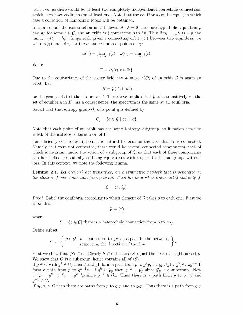
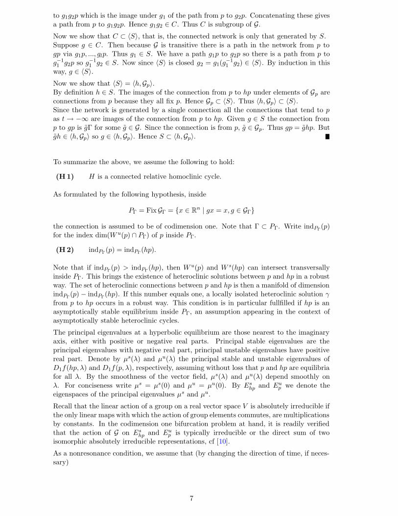
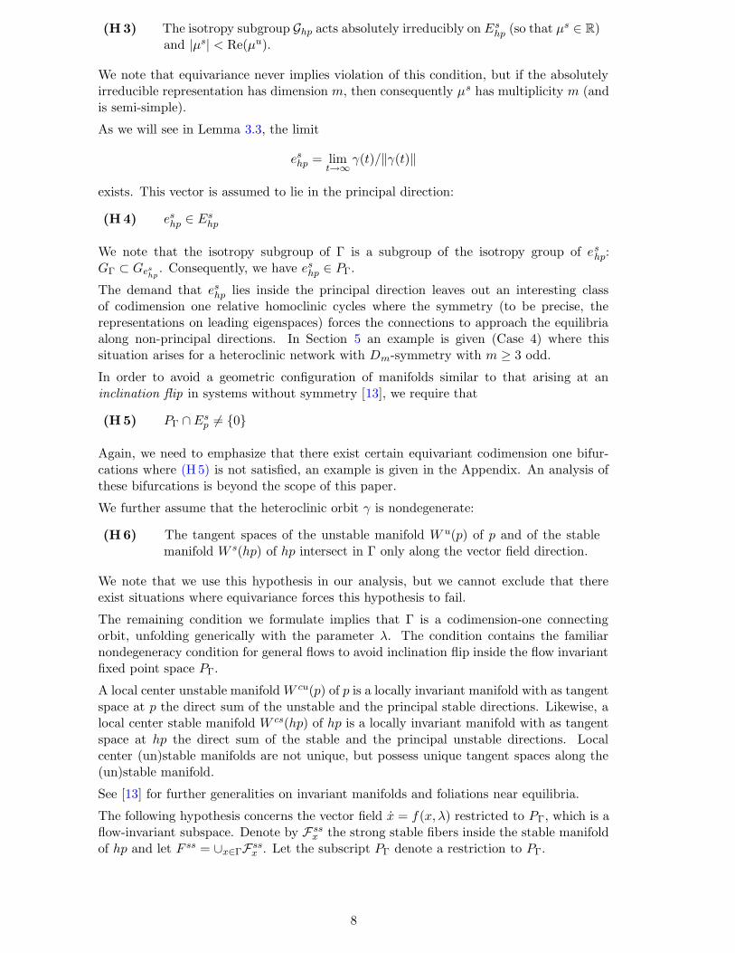
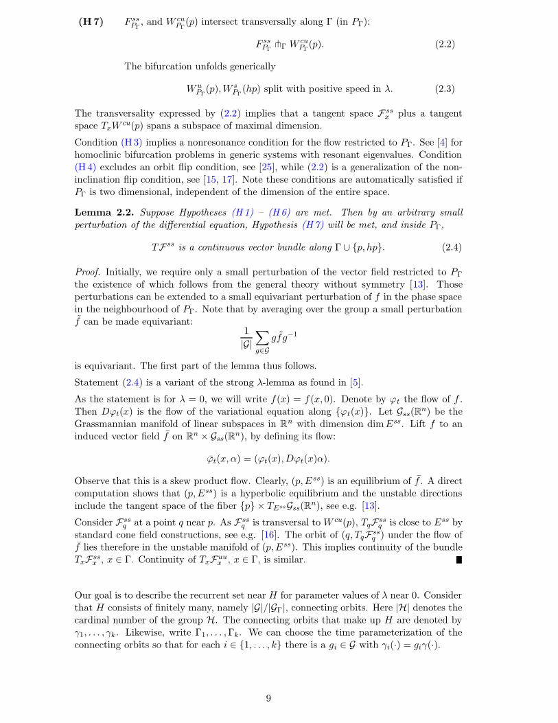


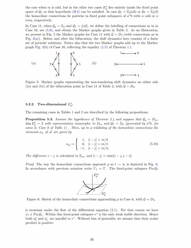
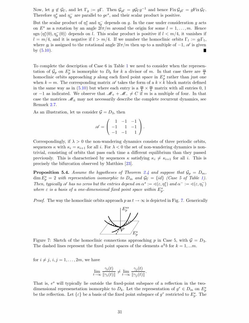


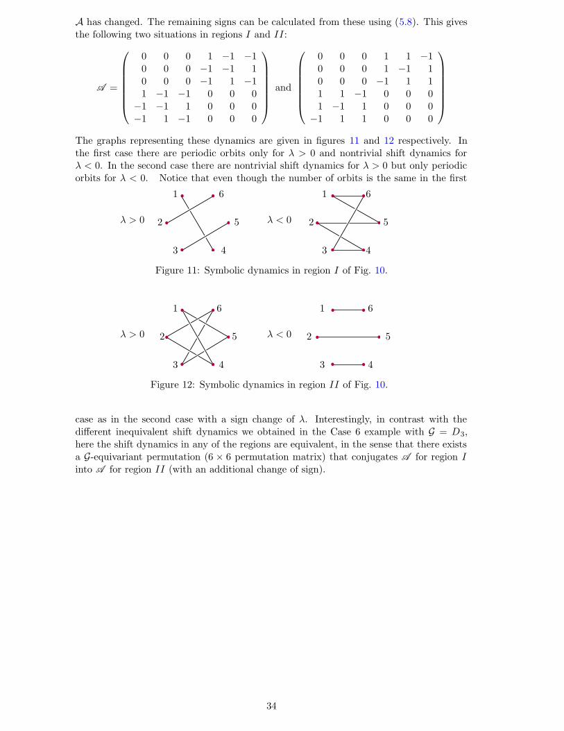


![0)1''2)$3(-4&56(42- 7)-+&3$)4* 0))1'&%,$)4*'$4'#2)5) · Using a discretization as in [9] and numerical bifurcation analysis, bifurcation curves are computed in section 3. A codimension](https://static.documents.pub/doc/80x56/5f43a7946b217b41644622d1/0123-45642-7-34-014425-using-a-discretization.jpg)


