154
BIS Quarterly Review December 2019 International banking and financial market developments BIS

BIS Quarterly Review
December 2019
International banking and financial market developments
BIS

BIS Quarterly Review Monetary and Economic Department Editorial Committee:
Claudio Borio Stijn Claessens Benoît Mojon Hyun Song Shin Philip Wooldridge
General queries concerning this commentary should be addressed to Philip Wooldridge (tel +41 61 280 8006, e-mail: [email protected]), queries concerning specific parts to the authors, whose details appear at the head of each section, and queries concerning the statistics to Patrick McGuire (tel +41 61 280 8921, e-mail: [email protected]).
This publication is available on the BIS website (www.bis.org/publ/qtrpdf/r_qt1912.htm).
© Bank for International Settlements 2019. All rights reserved. Brief excerpts may be
reproduced or translated provided the source is stated. ISSN 1683-0121 (print) ISSN 1683-013X (online)

BIS Quarterly Review, December 2019 iii
BIS Quarterly Review
December 2019
International banking and financial market developments
Easing trade tensions lift sentiment ........................................................................................... 1 Lingering worries initally keep markets range-bound .............................................. 2 Easing tensions drive up sentiment and asset prices ................................................ 4 Asset valuations reflect a low term premium ............................................................... 7 Box: September stress in dollar repo markets: passing or structural? .............. 12
Special features
FX and OTC derivatives markets through the lens of the Triennial Survey ............. 15 Philip Wooldridge
Offshore markets propel trading growth .................................................................... 15 Electronification is reshaping markets .......................................................................... 17 Compression and clearing mitigate exposures .......................................................... 18
Sizing up global foreign exchange markets ........................................................................ 21 Andreas Schrimpf and Vladyslav Sushko
FX trading volumes mostly reflect financial motives .............................................. 22 Zooming in on FX swaps .................................................................................................... 24 Trading with financial clients and FX prime brokerage .......................................... 28 Box A: FX prime brokerage and its contribution to trading volumes ............... 30 Electronification of trading across key market segments ..................................... 32 Concentration of FX trading in offshore hubs ........................................................... 33 Conclusion ............................................................................................................................... 34 Box B: Renminbi turnover tilts onshore ........................................................................ 35 Annex table .............................................................................................................................. 38
FX trade execution: complex and highly fragmented ...................................................... 39 Andreas Schrimpf and Vladyslav Sushko
An increasingly complex and fragmented market structure ............................... 40 Mapping out trade execution using the Triennial Survey ..................................... 41 How is the landscape of FX trade execution evolving? .......................................... 42
iv BIS Quarterly Review, December 2019
Conclusion ............................................................................................................................... 47 Box: FX settlement risk remains significant ................................................................. 48 Annex table .............................................................................................................................. 51
Offshore markets drive trading of emerging market currencies ................................. 53 Nikhil Patel and Dora Xia
Growth of FX trading in EME currencies ....................................................................... 54 Box A: FX instruments dominate derivatives markets in EMEs ........................... 56 Evolving market structure ................................................................................................... 57 Box B: NDF markets thrive on the back of electronification ................................ 61 Policy implications ................................................................................................................ 62 Box C: How onshore and offshore markets interact:
an empirical investigation .............................................................................. 63 Annex tables ............................................................................................................................ 66
The evolution of OTC interest rate derivatives markets ................................................. 69 Torsten Ehlers and Bryan Hardy
A broad-based rise in turnover ........................................................................................ 70 What drove the increase in turnover? ........................................................................... 71 Box: The shift to central clearing of OTC interest rate products ........................ 77 The increasing importance of OTC markets ............................................................... 80 Conclusion ............................................................................................................................... 81
OTC derivatives: euro exposures rise and central clearing advances ........................ 83 Sirio Aramonte and Wenqian Huang
Trends across countries and currencies ........................................................................ 84 Central clearing shaped patterns in derivatives outstanding ............................... 87 Conclusion ............................................................................................................................... 91 Box: Costs and benefits of switching to central clearing ....................................... 92
Euro repo market functioning: collateral is king ............................................................... 95 Angelo Ranaldo, Patrick Schaffner and Kostas Tsatsaronis
Trends in transaction volumes .......................................................................................... 96 Liquidity and pricing efficiency ......................................................................................... 98 Box: Measures of market liquidity and pricing efficiency .................................... 100 Arbitrage across segments ............................................................................................. 104 Specialisation of market participants ......................................................................... 106 Conclusion ............................................................................................................................ 107

BIS Quarterly Review, December 2019 v
BIS statistics: charts ................................................................................................................ A1
Notations used in this Review
billion thousand million e estimated lhs, rhs left-hand scale, right-hand scale $ US dollar unless specified otherwise … not available . not applicable – nil or negligible Differences in totals are due to rounding. The term “country” as used in this publication also covers territorial entities that are not states as understood by international law and practice but for which data are separately and independently maintained.

vi BIS Quarterly Review, December 2019
Abbreviations
Currencies ALL Albanian lek MXN Mexican peso ARS Argentine peso MXV Mexican unidad de inversión (UDI) AUD Australian dollar MYR Malaysian ringgit BGN Bulgarian lev NAD Namibian dollar BHD Bahraini dinar NGN Nigerian naira BRL Brazilian real NOK Norwegian krone CAD Canadian dollar NZD New Zealand dollar CHF Swiss franc OTH All other currencies CLP Chilean peso PEN Peruvian sol CNY (RMB) Chinese yuan (renminbi) PHP Philippine peso COP Colombian peso PLN Polish zloty CZK Czech koruna RON Romanian leu DKK Danish krone RUB Russian rouble EUR euro SAR Saudi riyal GBP pound sterling SEK Swedish krona HKD Hong Kong dollar SGD Singapore dollar HUF Hungarian forint THB Thai baht IDR Indonesian rupiah TRY Turkish lira ILS Israeli new shekel TWD New Taiwan dollar INR Indian rupee USD US dollar ISK Icelandic króna VES bolívar soberano JPY Japanese yen VND Vietnamese dong KRW Korean won XOF CFA franc (BCEAO) MAD Moroccan dirham ZAR South African rand

BIS Quarterly Review, December 2019 vii
Countries AE United Arab Emirates CY Cyprus AF Afghanistan CZ Czech Republic AL Albania DE Germany AM Armenia DJ Djibouti AO Angola DK Denmark AR Argentina DM Dominica AT Austria DO Dominican Republic AU Australia DZ Algeria AZ Azerbaijan EA euro area BA Bosnia and Herzegovina EC Ecuador BD Bangladesh EE Estonia BE Belgium EG Egypt BF Burkina Faso ER Eritrea BG Bulgaria ES Spain BH Bahrain ET Ethiopia BI Burundi FI Finland BJ Benin FJ Fiji BM Bermuda FO Faeroe Islands BN Brunei FR France BO Bolivia GA Gabon BR Brazil GB United Kingdom BS The Bahamas GD Grenada BT Bhutan GE Georgia BY Belarus GH Ghana BZ Belize GN Guinea CA Canada GQ Equatorial Guinea CD Democratic Republic of the Congo GR Greece CF Central African Republic GT Guatemala CG Republic of Congo GW Guinea-Bissau CH Switzerland GY Guyana CI Côte d’Ivoire HN Honduras CL Chile HK Hong Kong SAR CM Cameroon HR Croatia CN China HT Haiti CO Colombia HU Hungary CR Costa Rica ID Indonesia CV Cabo Verde IE Ireland

viii BIS Quarterly Review, December 2019
Countries (cont) IL Israel MX Mexico IN India MY Malaysia IQ Iraq MZ Mozambique IR Iran NA Namibia IS Iceland NC New Caledonia IT Italy NG Nigeria JE Jersey NL Netherlands JM Jamaica NO Norway JO Jordan NR Nauru JP Japan NZ New Zealand KE Kenya OM Oman KG Kyrgyz Republic PA Panama KH Cambodia PE Peru KR Korea PG Papua New Guinea KW Kuwait PH Philippines KY Cayman Islands PK Pakistan KZ Kazakhstan PL Poland LA Laos PT Portugal LB Lebanon PY Paraguay LC St Lucia QA Qatar LK Sri Lanka RO Romania LR Liberia RS Serbia LS Lesotho RU Russia LT Lithuania RW Rwanda LU Luxembourg SA Saudi Arabia LV Latvia SC Seychelles LY Libya SD Sudan MA Morocco SE Sweden MD Moldova SG Singapore ME Montenegro SK Slovakia MH Marshall Islands SI Slovenia MK North Macedonia SR Suriname ML Mali SS South Sudan MM Myanmar ST São Tomé and Príncipe MN Mongolia SV El Salvador MO Macao SAR SZ Eswatini MR Mauritania TD Chad MT Malta TG Togo MU Mauritius TH Thailand MV Maldives TJ Tajikistan MW Malawi TL East Timor

BIS Quarterly Review, December 2019 ix
Countries (cont) TM Turkmenistan VC St Vincent and the Grenadines TO Tonga VE Venezuela TR Turkey VG British Virgin Islands TT Trinidad and Tobago VN Vietnam TW Chinese Taipei XM euro area UA Ukraine ZA South Africa US United States ZM Zambia UY Uruguay 1C International organisations UZ Uzbekistan 1Z British West Indies
BIS Quarterly Review, December 2019 1
Easing trade tensions lift sentiment
An easing of US-China trade tensions in October triggered a risk-on phase in global financial markets.1 In September, risky asset prices across the globe stayed range-bound, supported by additional monetary accommodation in a context of subdued prospects for global activity. As sentiment shifted, stocks posted large gains in most markets but China, and credit spreads tightened. Term spreads in advanced economies (AEs) initially widened in line with the change in market sentiment. But their upward momentum petered out after a few weeks.
Faced with persistently low inflation and a still tepid outlook for growth, central banks eased further in several major economies. Policy rates were lowered in the United States, the euro area and a number of emerging market economies (EMEs), including Brazil, China, Indonesia and Mexico. The ECB restarted its programme of government bond purchases.
As sentiment shifted with more constructive developments in the US-China relationship (and better prospects for an orderly Brexit), equities rose across the globe, with the notable exception of Chinese stocks, which lost ground in October and November. In the United States, stock prices reached historically high levels, with risk appetite spurred by a still resilient consumer sector, early signs of stabilisation in manufacturing and earnings reports that came in line with – or slightly ahead of – expectations. Sentiment was also helped by still patchy evidence in October’s activity gauges that several economies, advanced and emerging, were bottoming out.
Corporate spreads fell globally and long-term sovereign yields rose in AEs. Spreads on euro area and US corporate bonds declined, especially for investment grade issuers. In the high-yield segment, and also EME corporates, spreads widened in late September but compressed again in mid-October as the news turned more positive. Government bond yields rose, steepening yield curves, but long bond yields traced back some of their gains in November.
As the demand for safe assets retreated, the US dollar weakened broadly, in particular against EME currencies. EME sovereign yields, little affected by sentiment swings, continued on the downward trend that prevailed for most of the year.
Loose financial conditions intensified the focus on the sustainability of asset valuations. Corporate bonds appeared relatively expensive, particularly in the light of the still comparatively subdued economic outlook. Equity valuations seemed high in the United States compared with historical averages, but were moderate in most other countries and relative to sovereign yields. However, investors’ compensation for bearing equity risk seems to hinge on the term premium; to the extent that the premium is unusually low, it may flatter valuations.
1 The period under review extends from 12 September to 27 November 2019.
2 BIS Quarterly Review, December 2019
Lingering worries initially keep markets range-bound
Financial markets mainly reflected the ebb and flow of trade tensions during the period under review. Early on, sentiment stayed subdued and risky assets traded sideways, as investors continued to struggle with the uncertain outlook stemming from enduring US-China tensions and lingering signs of weakness in manufacturing. Faced with a deteriorating macroeconomic outlook, central banks in several jurisdictions chose to provide further monetary accommodation.
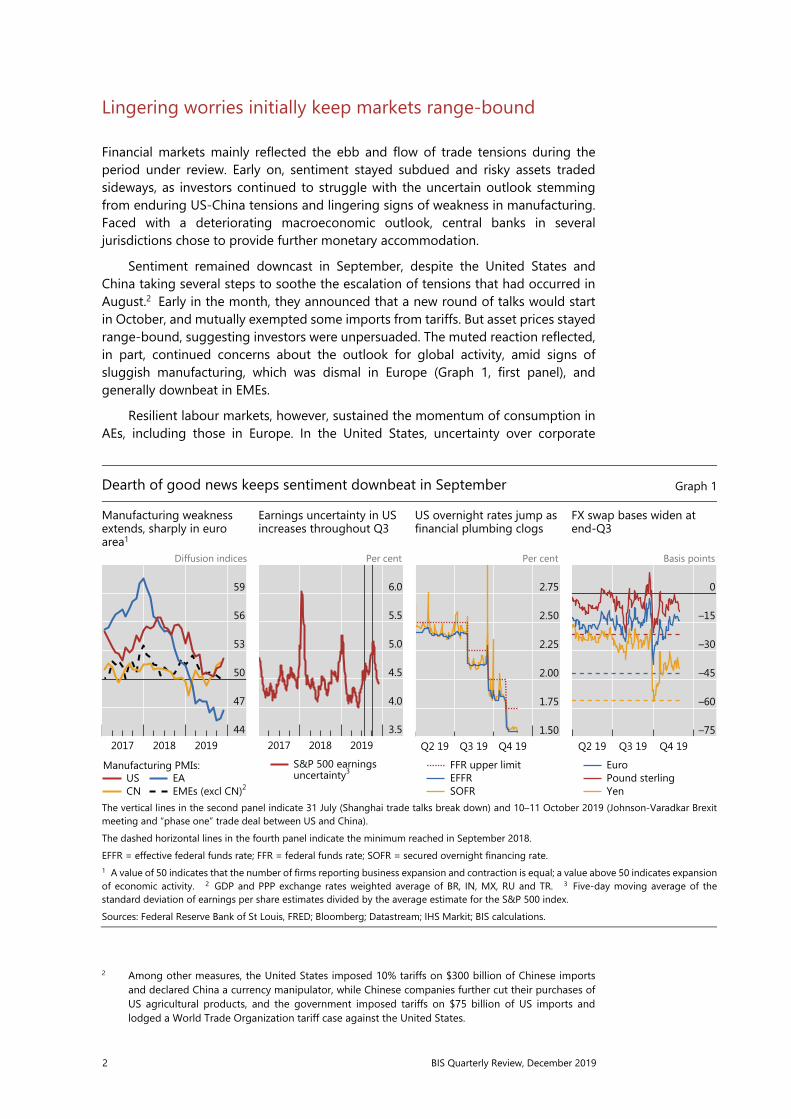
Sentiment remained downcast in September, despite the United States and China taking several steps to soothe the escalation of tensions that had occurred in August.2 Early in the month, they announced that a new round of talks would start in October, and mutually exempted some imports from tariffs. But asset prices stayed range-bound, suggesting investors were unpersuaded. The muted reaction reflected, in part, continued concerns about the outlook for global activity, amid signs of sluggish manufacturing, which was dismal in Europe (Graph 1, first panel), and generally downbeat in EMEs.
Resilient labour markets, however, sustained the momentum of consumption in AEs, including those in Europe. In the United States, uncertainty over corporate
2 Among other measures, the United States imposed 10% tariffs on $300 billion of Chinese imports
and declared China a currency manipulator, while Chinese companies further cut their purchases of US agricultural products, and the government imposed tariffs on $75 billion of US imports and lodged a World Trade Organization tariff case against the United States.
Dearth of good news keeps sentiment downbeat in September Graph 1
Manufacturing weakness extends, sharply in euro area1
Earnings uncertainty in US increases throughout Q3
US overnight rates jump as financial plumbing clogs
FX swap bases widen at end-Q3
Diffusion indices Per cent Per cent Basis points
The vertical lines in the second panel indicate 31 July (Shanghai trade talks break down) and 10–11 October 2019 (Johnson-Varadkar Brexit meeting and “phase one” trade deal between US and China). The dashed horizontal lines in the fourth panel indicate the minimum reached in September 2018. EFFR = effective federal funds rate; FFR = federal funds rate; SOFR = secured overnight financing rate. 1 A value of 50 indicates that the number of firms reporting business expansion and contraction is equal; a value above 50 indicates expansion of economic activity. 2 GDP and PPP exchange rates weighted average of BR, IN, MX, RU and TR. 3 Five-day moving average of the standard deviation of earnings per share estimates divided by the average estimate for the S&P 500 index. Sources: Federal Reserve Bank of St Louis, FRED; Bloomberg; Datastream; IHS Markit; BIS calculations.
59
56
53
50
47
44201920182017
USCN
Manufacturing PMIs:EAEMEs (excl CN)2
6.0
5.5
5.0
4.5
4.0
3.5201920182017
S&P 500 earningsuncertainty3
2.75
2.50
2.25
2.00
1.75
1.50Q4 19Q3 19Q2 19
FFR upper limitEFFRSOFR
0
–15
–30
–45
–60
–75Q4 19Q3 19Q2 19
EuroPound sterlingYen

BIS Quarterly Review, December 2019 3
earnings prospects, growing pari passu with trade tensions (Graph 1, second panel), also contributed to keeping equities flat throughout the third quarter.
Other developments in September were not reassuring. Throughout the month, a fluid political situation in the United Kingdom appeared, at first, to strengthen the likelihood of a “no-deal” Brexit. In mid-September, oil prices jumped by almost 15% after an attack on oil facilities in Saudi Arabia. This was the largest daily spike in oil prices in almost 20 years, but prices fell back again within days.
Also in September, sudden stress in the US repo market raised concerns about the fragility of US dollar funding markets (see box). The benchmark repo rate (secured overnight financing rate, SOFR) more than doubled for a day, and the effective federal funds rate overshot the upper limit of the Federal Reserve’s policy range (Graph 1, third panel). Actions by the Federal Reserve returned calm to this market, and the dislocation did not spread. However, the bases of major currency FX swaps, another key funding market, plummeted at the quarter-end, in a repeat of the stress observed the previous September (fourth panel). Observers worried about the prospects of renewed dislocations in these markets as the year-end approached.
Confronted with the combination of tepid activity and persistent low inflation, central banks in major economies eased monetary policy further. On 12 September, the ECB announced the resumption of the government bond purchase programme, a 10 basis point reduction in the deposit rate, lower rates for the longer-term refinancing operations and a new system of tiered remuneration of bank reserves to contain the effect of more negative interest rates on bank profitability. The Federal Reserve cut its policy rate twice, in September and October, in line with market expectations, but signalled that more reductions this year were unlikely. Nevertheless, forward rates indicated expectations of further declines in policy rates in 2020 (Graph 2, first panel).
Major central banks ease further before sentiment turns Graph 2
Policy rates and expectations drop1
Term spreads rebound as tensions ease
Real rates, term premium drive US long yields
EME sovereign yields and spreads drop further
Per cent Basis points Per cent Per cent Basis points
The vertical lines indicate 31 July (Shanghai trade talks break down) and 10–11 October 2019 (Johnson-Varadkar Brexit meeting and “phase one” trade deal between US and China). ACM = Adrian, Crump and Moench. 1 The dashed lines indicate expected rates based on overnight index swap (OIS) forward rates; as of28 November 2019. 2 Deposit facility rate. 3 Interest rate applied to policy rate balances in current accounts that financial institutionshold at the Bank of Japan. 4 Federal funds rate. 5 JPMorgan Chase EMBI Global index. 6 JPMorgan Chase GBI-EM index. Sources: T Adrian, R Crump and E Moench, “Pricing the term structure with linear regressions”, Journal of Financial Economics, vol 110, no 1, 2013; Federal Reserve Bank of New York; Bloomberg; Datastream; JPMorgan Chase; national data; BIS calculations.
2
1
0
–120202019
EA2 JP3 US4
60
30
0
–30Q4 19Q2 19
DE10 yr–2 yr govt bond spread:
JP
US
0.75
0.00
–0.75
–1.50Q4 19Q2 19
10 yr TIPS10 yr ACM term premium
6.5
5.5
4.5
3.5
450
400
350
300Q4 19Q2 19
USD5
Local currency6
Yields (lhs):
Spread (rhs):

4 BIS Quarterly Review, December 2019
Several other central banks in AEs and EMEs echoed moves by the Fed and the ECB. In late September and throughout October, Australia, Brazil, India, Korea, Mexico, Russia and Turkey lowered their policy rates. After keeping interbank rates broadly stable for most of the year, the People’s Bank of China (PBC) cut its one-year rate in early November, and then its seven-day interbank rate mid-month. Observers disagreed on the future path of monetary policy, as the PBC faced several challenges, including a perceived commitment to the deleveraging of the economy, weak economic activity, some degree of stress in local banks and rising inflation as food pushed consumer prices up. The Bank of Japan stayed on the sidelines, on the back of its assessment about the Japanese economy’s prospects.
Easing tensions drive up sentiment and asset prices
An easing of geopolitical tensions during the first half of October set the stage for a turn in market sentiment. Moreover, tentative signs of stabilisation in global activity started to emerge. With prospects improving for both a Brexit deal and a sustained truce in trade tensions between the United States and China, a wave of risk appetite took hold of markets.
The mood started to improve in mid-October. After a meeting of the UK and Irish prime ministers on 10 October defused concerns of a “no-deal” Brexit, sterling regained some ground. The following day, the announcement of a limited “phase one” deal between China and the United States marked an inflexion point for asset prices. The rally was further spurred by tentative clues that economic activity in several countries had bottomed out: manufacturing PMIs appeared to bounce back modestly in the United States, and new manufacturing orders in Germany improved, though PMIs in Europe and other AEs remained less upbeat. In EMEs the picture was mixed, pointing to regional cleavages: conditions appeared to improve in an Asian bellwether like Chinese Taipei, but survey data from Korea and Malaysia still lagged. In Latin America, Brazil continued posting moderate yet solid activity numbers, but Mexico remained less dynamic. Emerging Europe was still fairly weak. In the United States, the concerns about earnings were dispelled by reports that generally came out in line with – or slightly above – expectations.
Government bond markets in AEs reacted, initially, in risk-on fashion. After flattening most of the year, yield curves steepened, mainly as a result of increases at the long end (Graph 2, second panel). In the United States, the upswing was driven in part by higher real long-term rates, as indicated by higher yields of Treasury Inflation-protected Securities (TIPS), a market gauge of real rates (third panel, blue line). Yields on 10-year TIPS had been steady since early October, possibly signalling investor confidence in a rebound in activity. The term premium embedded in the yield of the 10-year Treasury nominal benchmark also increased from historical lows – though it stayed negative – suggesting that an upward shift in risk appetite was part of the explanation (third panel, red line). Yet long yields did not sustain the upward momentum, and traced back some of their gains as November moved on.
Sovereign yields in EMEs, for debt denominated both in US dollars and local currency, continued on the downward path that dominated this year (Graph 2, fourth panel, green and red solid lines, respectively). EME yields have been gradually decreasing since the Federal Reserve’s policy pivot began last November. The trend steepened especially after the Fed Chairman indicated in June that the central bank would act as appropriate to sustain the expansion in the face of economic challenges,

BIS Quarterly Review, December 2019 5
including those emerging from trade disputes.3 Irrespective of still patchy evidence of economic rebound, EME yields were at their lowest levels since 2014.
EME sovereign spreads against US Treasury benchmarks for US dollar-denominated debt also narrowed further, again approaching post-Great Financial Crisis (GFC) lows (Graph 2, fourth panel, dotted green line). Spreads had recently been more volatile than yields, but most of that volatility stemmed from wide fluctuations in US Treasury benchmarks, not in EME yields. These patterns suggested that, in an unusual reversal, swings in market sentiment had a more pronounced effect in the pricing of AE fixed income. Rising EME government debt, which has surpassed 50% of GDP on the global average and was on its way to surpassing 70% of GDP in some regions by year-end,4 did not deter investors: not only emerging market but also frontier, or pre-emerging market, economies were able to place large amounts of debt this year (see next section).
In October, stock markets broke out of the range in which they had been trading since mid-year. Benchmarks in advanced and emerging market economies other than China touched year highs in November (Graph 3, first panel). In the United States, the major stock indices reached new all-time peaks. With investors seemingly convinced that the economic and trade outlook had improved, forward-looking gauges of stock market volatility approached their minima for the year (second panel) and net short
3 See BIS, “Markets swing on trade and monetary policy”, BIS Quarterly Review, September 2019,
pp 1–14. 4 See the Methodological and Statistical Appendix in International Monetary Fund, Fiscal monitor: How
to mitigate climate change, October 2019.
Risk appetite returns to most equity markets as tensions subside Graph 3
US equities reach all-time highs1
Volatilities approach year lows
Investors’ short volatility positions reach all-time peak
Investors’ anticipate less downside in EME stocks
1 May 2019 = 100 % pts ‘000 contracts Millions of contracts
The vertical lines indicate 31 July (Shanghai trade talks break down) and 10–11 October 2019 (Johnson-Varadkar Brexit meeting and “phase one” trade deal between US and China). The dashed horizontal lines in the second panel indicate averages over the period 2002–06. 1 GDP weighted averages across regional economies. 2 Shanghai composite equity index. 3 Implied volatility of the EURO STOXX 50 andNikkei 225 indices; weighted average based on market capitalisation. 4 Non-commercial. 5 iShares MSCI Emerging Markets ETF. Sources: IMF, World Economic Outlook; Bloomberg; BIS calculations.
108
104
100
96
92
88Q4 19Q3 19Q2 19
United StatesAEs excl US1
EMEs excl CN1
China2
25
22
19
16
13
102019
CBOE VIX IndexOther AE stock markets3
0
–50
–100
–150
–200
–2502019
Net long positionsin VIX futures4
0
–1
–2
–3
–4
–52019
EME5Open interest, call-put:

6 BIS Quarterly Review, December 2019
speculative positions on VIX futures also reached an all-time high, pointing to investors’ renewed appetite for risk (third panel). Improved sentiment about EMEs carried over to option markets, where investors moved away from positions that would protect them from downside risk (fourth panel). Yet the contrast with the restrained response of Chinese stock markets and the still limited evidence of a rebound in global activity begged the question of whether stock prices might be running ahead of themselves in some markets.
Corporate spreads tightened across credit rating categories. Investment grade in the United States and Europe (Graph 4, left-hand panel) and EME corporate debt (centre panel, yellow line) rallied in October and their spreads also approached minima for the year. While it had been broadly stable over the past three years, corporate debt in EMEs remained relatively high, with credit to non-financial corporates around 100% of GDP. Corporate bond spreads continued to be sensitive to developments in trade tensions. In particular, US and European high-yield spreads tightened in October, after widening in September on still disappointing economic data and simmering trade tensions. That said, spreads stayed slightly above the troughs reached earlier in the year and clearly below long-term averages (centre panel, blue and red lines).
On balance, financial conditions eased further in both the United States and Europe (Graph 4, right-hand panel). In fact, with the exception of a temporary trade tension-induced deterioration in May, financial conditions had been improving since the beginning of 2019. In the United States, they were back to levels similar to those before market volatility spiked in the fourth quarter of 2018. In the euro area, financial conditions were more supportive than they had been since early 2018.
Corporate credit spreads remain tight, and overall financial conditions loose Graph 4
Investment grade High-yield and EMEs Financial conditions remain accommodative3
Basis points Basis points Index
The vertical lines indicate 31 July (Shanghai trade talks break down) and 10–11 October 2019 (Johnson-Varadkar Brexit meeting and “phase one” trade deal between US and China). The dashed horizontal lines in the left-hand and centre panels indicate long-term averages (2005–current). 1 Option-adjusted spreads. 2 JPMorgan CEMBI index; stripped spread. 3 100 indicates country-specific long-term averages; each unit above (below) 100 denotes financial conditions that are one standard deviation tighter (looser) than the average. Sources: Bloomberg; Goldman Sachs; ICE BoAML indices; JPMorgan Chase; BIS calculations.
160
140
120
100
802019
United StatesInvestment grade corporate spreads:1
Europe
525
450
375
300
2252019
High-yield US1
High-yield Europe1
Corporate spreads:EMEs2
100.0
99.4
98.8
98.2
97.620192018
United States Euro area

BIS Quarterly Review, December 2019 7
As the risk-on phase in markets gained momentum and safe asset demand retreated, the US dollar weakened. The greenback had lost some ground against EME currencies even before the announcement of the phase one trade deal between China and the United States. But the depreciation became broad-based – including against other AE currencies – after this announcement (Graph 5, left-hand panel). Other traditional safe haven currencies like the yen and the Swiss franc stayed flat or even depreciated vis-à-vis the US currency. In a further sign that risk appetite had turned, riskier EME currencies, which normally rise together with returns on carry trade strategies, gained in October more than the trade weighted benchmark (centre panel). Forward-looking gauges of FX volatility dropped to lows for the year, possibly reflecting the expectation of a sustained truce in US-China tensions (right-hand panel).
Asset valuations reflect a low term premium
As the risk-on phase set in and bond yields edged up, the term premium remained negative – something unique to the post-crisis period. The premium has been declining for about 30 years alongside bond yields. The current debate about the underlying drivers of this trend and likely persistence of the low level has heightened uncertainty about asset valuations.5 A commonly used gauge of the compensation
5 For a recent discussion of developments in the term premium, see R Clarida, “Monetary policy, price
stability, and equilibrium bond yields: success and consequences”, remarks at the High-Level Conference on Global Risk, Uncertainty, and Volatility, Zurich, November 2019. He stresses that, given
EME currencies strengthen vis-à-vis the dollar as risk appetite increases Graph 5
EME currencies strengthen Stronger gains for carry trade currencies in October
FX implied volatilities drop to lowest level in three years5
2 Jan 2019 = 100 Per cent Percentage points
The vertical line in the left-hand panel indicates 10–11 October 2019 (Johnson-Varadkar Brexit meeting and “phase one” trade deal betweenUS and China). The dashed horizontal lines in the right-hand panel indicate long-term averages (2000–current). 1 Goods and services. 2 A positive value indicates that the local currency has appreciated against the US dollar. 3 Beta of a univariate regression of the exchange rate vis-à-vis the US dollar and the Bloomberg Cumulative FX Carry Trade Index for eight EME currencies for theperiod 9 October 2016–9 October 2019. High = larger than the median. 4 Multiplied by –1. OITP = other important trading partners. 5 JPMorgan Chase implied volatility indices. 6 Based on JPMorgan Chase G7 currencies implied volatility index. Sources: Federal Reserve Bank of St Louis, FRED; Bloomberg; BIS calculations.
103.0
101.5
100.0
98.5
97.02019
Advanced foreign economiesEMEs
Trade-weighted USD index:1
INMYTHTWCNPEPHIDTRSGBR
OITPRUCOKRCZPL
MXHUZA
3210
High-beta currencies3
Low-beta currencies3
USD trade-weighted4
FX change, 9–25 Oct 2019:2
12
10
8
6
4201920182017
AE currencies6 EME currencies

8 BIS Quarterly Review, December 2019
that investors earn for bearing risk compares the yield on risky assets with that on government bonds. A compressed term premium depresses government bond yields and thus, to the extent that the premium is unusually low, it may flatter valuations. If the term premium is removed, certain assets appear to offer limited risk compensation.
In equity markets, there were noticeable differences in valuations across countries. Valuations were elevated in France and the United States, where in late 2019 the cyclically adjusted price/earnings (CAPE) ratio was higher than in 89% and 86% of the months since 2010, respectively. In other countries, including Germany but particularly China and Japan, CAPE ratios were closer to the bottom of their respective post-GFC ranges (Graph 6, left-hand panel).
Equity valuations appear more subdued when accounting for low interest rates, in the sense that returns on equities appear to offer a sizeable compensation for risk. The earnings yield, or the inverse of the CAPE ratio, had declined steadily in the United States from the GFC until late 2017, indicating that investors paid increasingly higher prices for US equities given profitability levels (Graph 6, centre panel, red line). Since 2018, the earnings yield has slowly inched up, pointing to slightly decreasing valuations. However, the spread between the earnings yield and the 10-year Treasury yield – a valuation gauge that measures the compensation earned by investors for holding equity risk – stood at about the historical norm in late 2019 (centre panel, blue line). The level of this spread suggests that equities were not particularly expensive given the level of interest rates, and that investors were earning similar compensation for equity risk as in the past.
that the returns on bonds and stocks have become negatively correlated over the last two decades, the explanation for low and even negative term premia could be that bonds have become a hedge for stocks.
US equity valuations hinge on the compressed term premium Graph 6
US equity valuations are elevated1 The US earnings yield spread is due to the low term premium
Similar patterns emerge in France
Percentiles Per cent Percentage points Per cent Percentage points
1 For the US, Robert Shiller data until November 2019; for other countries, Barclays Shiller CAPE ratios until September 2019. 2 Relative to the distribution of country-specific monthly Shiller CAPE ratios between 2010 and present. 3 Inverted Shiller CAPE ratio. 4 Using expected nominal 10-year rate component of Hördahl and Tristani term premium. Sources: P Hördahl and O Tristani, “Inflation risk premia in the euro area and the United States”, International Journal of Central Banking, vol 10, no 3, 2014; R Shiller, www.econ.yale.edu/~shiller/data.htm; Barclays; Bloomberg; BIS calculations.
100
75
50
25
0
CNJPDEFRUS
High valuations
Low valuations
Last available dataShiller CAPE ratio (percentiles):2
6
4
2
0
–2
6
4
2
0
–2
1917151311
Earnings yield3Lhs:
10-yr yield spreadEarnings–US Treasury
Earnings–expected nominal10-yr yield spread4
Rhs:
8
6
4
2
0
8
6
4
2
0
1917151311
Earnings yield3Lhs:Earnings–10-yr yield spreadEarnings–expected nominal10-yr yield spread4
Rhs:

BIS Quarterly Review, December 2019 9
However, such compensation would be less benign if adjusted for the low level of the term premium. Not only was the improvement in valuations almost fully due to interest rates, it was largely driven by the decline of the term premium, which is a fairly volatile component of interest rates. The earnings yield spread relative to the expected nominal US Treasury rate – that is, after removing the term premium from interest rates – was quite low by historical standards (Graph 6, centre panel, yellow line). In fact, it suggested that investors were receiving little compensation for equity risk. Similar patterns could be observed for French equities (right-hand panel).
Valuations in US commercial real estate (CRE) markets also seem to hinge on the low level of the term premium. The capitalisation rate (cap rate), calculated as property income over purchase price, is a common measure of CRE valuations. In October, cap rates were compressed, indicating stretched valuations, with the exception of retail properties, whose prices reflected adverse shifts in shopping patterns in favour of online retail (Graph 7, all panels, left-most bars). Like the earnings yield spread for equities, the cap rate spread over the 10-year US Treasury yields suggested much lower valuations, somewhat below the historical norm (all panels, centre bars). As for equities, however, much of the difference in valuations was due to the low term premium, and cap rate spreads over expected nominal rates were compressed and close to the bottom of the post-GFC range, indicating that the recent decline of the term premium was driving valuations (all panels, right-most bars).
In corporate bond markets, various indicators pointed to higher than average valuations. One simple measure is the corporate yield spread relative to government bonds of similar maturity. In late 2019, AE spreads were lower than they had been 80% of the time since 2010 in the investment grade segment (Graph 8, first panel). Valuations were closer to the average for EME and for AE high-yield corporate bonds, with spreads lower than they had been 70% of the time since 2010.
Commercial real estate valuations also largely depend on the term premium Capitalisation rates, as percentiles, October 20191 Graph 7
Apartment buildings Office buildings Retail buildings
1 Relative to a distribution of monthly values between 2010 and October 2019. 2 Spread of US market capitalisation rate to zero couponUS Treasury 10-year yield. 3 Spread of US market capitalisation rate to expected US Treasury 10-year yield. Sources: P Hördahl and O Tristani, “Inflation risk premia in the euro area and the United States”, International Journal of Central Banking, vol 10, no 3, 2014; Bloomberg; Real Capital Analytics; BIS calculations.
100
75
50
25
0
Cap
rate
Cap
rate
ove
r
Cap
rate
ove
r
10-y
r yie
ld2
10-y
r exp
ecte
d
rate
3
High valuations
Low valuations 100
75
50
25
0
Cap
rate
Cap
rate
ove
r
Cap
rate
ove
r
10-y
r yie
ld2
10-y
r exp
ecte
d
rate
3
Low valuations
High valuations
100
75
50
25
0
Cap
rate
Cap
rate
ove
r
Cap
rate
ove
r
10-y
r yie
ld2
10-y
r exp
ecte
d
rate
3
High valuations
Low valuations

10 BIS Quarterly Review, December 2019
Furthermore, in recent quarters corporate bond valuations showed signs of diverging from their traditional economic drivers. For example, euro area and US valuations appeared rich in relation to the outlook for manufacturing activity. Corporate bonds are often used to finance working capital and investment, and their valuations had tracked manufacturing PMIs closely since the GFC. In particular, periods of relatively strong prospects for manufacturing (ie high PMIs) corresponded to elevated corporate bond valuations in the form of compressed spreads, with a stronger link for US corporate bond spreads between 2016 and 2018 (Graph 8, second panel).
In early 2019, a gap had started opening between high corporate bond valuations and muted prospects for manufacturing activity. In November, this gap was the largest since 2013, indicating that corporate bond valuations were unusually buoyant relative to weak manufacturing. The divide was evident for investment grade and high-yield bonds in both the euro area and the United States (Graph 8, second and third panels).
The disconnect between corporate bond valuations and manufacturing activity was less pronounced in EMEs. While bond valuations were above their post-GFC midpoint, manufacturing PMIs were roughly at the middle of their range since 2010, instead of near the bottom as in the United States and euro area (Graph 8, fourth panel). As a result, corporate bond valuations in EMEs appeared more in line with the macroeconomic backdrop.
Corporate bond valuations were not driven by unusually low default risk. Global default rates for speculative grade bonds had been relatively steady for the past several years, picking up in 2016 but settling back in 2018 to levels similar to the
Corporate bond valuations are high globally All variables expressed as percentiles Graph 8
Corporate bonds are relatively expensive
Rich bond valuations contrast with weak manufacturing activity in the euro area…1
…and in the United States1 In EMEs, bond valuations are more in line with manufacturing activity1
1 Relative to a distribution of monthly values between 2010 and present. 2 For the United States and Europe, Bank of America Merrill Lynchcorporate bond index, option-adjusted spread; for EMEs, JPMorgan Chase CEMBI index, stripped spread. 3 JPMorgan Chase CEMBI, stripped spread. 4 GDP and PPP exchange rates weighted average of BR, CN, IN, MX, RU and TR, three-month moving average. Sources: IMF, World Economic Outlook; ICE BoAML indices; IHS Markit; JPMorgan Chase; BIS calculations.
100
75
50
25
0
US IG
US H
YEu
rope
IGEu
rope
HY
EMEs
High valuations
Low valuations
Sep–Oct 2019Corporate spreads (reversed):1, 2
100
75
50
25
0 100
75
50
25
0
19171513
Investment grade2
High-yield2
(lhs, reversed):Corporate spreads
100
75
50
25
0 100
75
50
25
0
19171513
Manufacturing PMIsRhs:
100
75
50
25
0 100
75
50
25
0
19171513
Corporate spreads(lhs, reversed)3
Manufacturing PMIs (rhs)4

BIS Quarterly Review, December 2019 11
2010–17 average (2.09% compared with 2.35%).6 In September and October, expected default risk and downgrades for US high-yield issuers rose to levels last seen in 2016.7
In a further sign of strong risk appetite, investor demand for higher-risk bonds remained high. The US market for high-yield bonds saw issuance of $34 billion in September, exceeding all monthly totals since January 2018 and well above the $23 billion monthly average between 2010 and 2017. Similarly, in October bond investment funds that focus on countries classified as frontier markets saw the second highest inflow over the previous 12 months. The total assets managed by these funds rose from $3.7 billion in November 2018 to $5.4 billion in October.
6 S&P Global Ratings, 2018 annual global corporate default and rating transition study, 2019. 7 Moody’s Analytics, “Worsened fundamentals lift downgrades well above upgrades”, 10 October 2019;
Moody’s Analytics, “Leading credit-risk indicator signals a rising default rate”, 5 September 2019.
12 BIS Quarterly Review, December 2019
September stress in dollar repo markets: passing or structural? Fernando Avalos, Torsten Ehlers and Egemen Eren
The mid-September tensions in the US dollar market for repurchase agreements (repos) were highly unusual. Repo rates typically fluctuate in an intraday range of 10 basis points, or at most 20 basis points. On 17 September, the secured overnight funding rate (SOFR) – the new, repo market-based, US dollar overnight reference rate – more than doubled, and the intraday range jumped to about 700 basis points. Intraday volatility in the federal funds rate was also unusually high. The reasons for this dislocation have been extensively debated; explanations include a due date for US corporate taxes and a large settlement of US Treasury securities. Yet none of these temporary factors can fully explain the exceptional jump in repo rates.
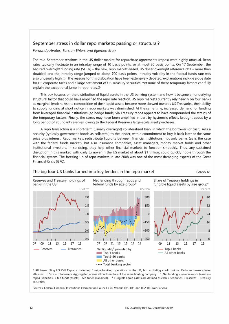
This box focuses on the distribution of liquid assets in the US banking system and how it became an underlying structural factor that could have amplified the repo rate reaction. US repo markets currently rely heavily on four banks as marginal lenders. As the composition of their liquid assets became more skewed towards US Treasuries, their ability to supply funding at short notice in repo markets was diminished. At the same time, increased demand for funding from leveraged financial institutions (eg hedge funds) via Treasury repos appears to have compounded the strains of the temporary factors. Finally, the stress may have been amplified in part by hysteresis effects brought about by a long period of abundant reserves, owing to the Federal Reserve’s large-scale asset purchases.
A repo transaction is a short-term (usually overnight) collateralised loan, in which the borrower (of cash) sells a security (typically government bonds as collateral) to the lender, with a commitment to buy it back later at the same price plus interest. Repo markets redistribute liquidity between financial institutions: not only banks (as is the case with the federal funds market), but also insurance companies, asset managers, money market funds and other institutional investors. In so doing, they help other financial markets to function smoothly. Thus, any sustained disruption in this market, with daily turnover in the US market of about $1 trillion, could quickly ripple through the financial system. The freezing-up of repo markets in late 2008 was one of the most damaging aspects of the Great Financial Crisis (GFC).
The big four US banks turned into key lenders in the repo market Graph A1
Reserves and Treasury holdings of banks in the US1
Net lending through repos and federal funds by size group2
Share of Treasury holdings in fungible liquid assets by size group4
USD trn USD bn Per cent
1 All banks filing US Call Reports, including foreign banking operations in the US, but excluding credit unions. Excludes broker-dealeraffiliates 2 Size = total assets. Aggregated across all bank entities of the same holding company. 3 Net lending = reverse repos (assets) –repos (liabilities) + fed funds (assets) – fed funds (liabilities). 4 Fungible liquid assets are defined as cash + fed funds + reserves + Treasurysecurities. Sources: Federal Financial Institutions Examination Council, Call Reports 031, 041 and 002; BIS calculations.
2.0
1.5
1.0
0.5
0.0
–0.519171513110907
Reserves Treasuries
300
150
0
–150
–300
–45019171513110907
Top 4 banksTop 5–30 banksAll other banksTotal banking sector
Net liquidity3 provided by:
40
32
24
16
8
0191715131109
Top 4 banksAll other banks
BIS Quarterly Review, December 2019 13
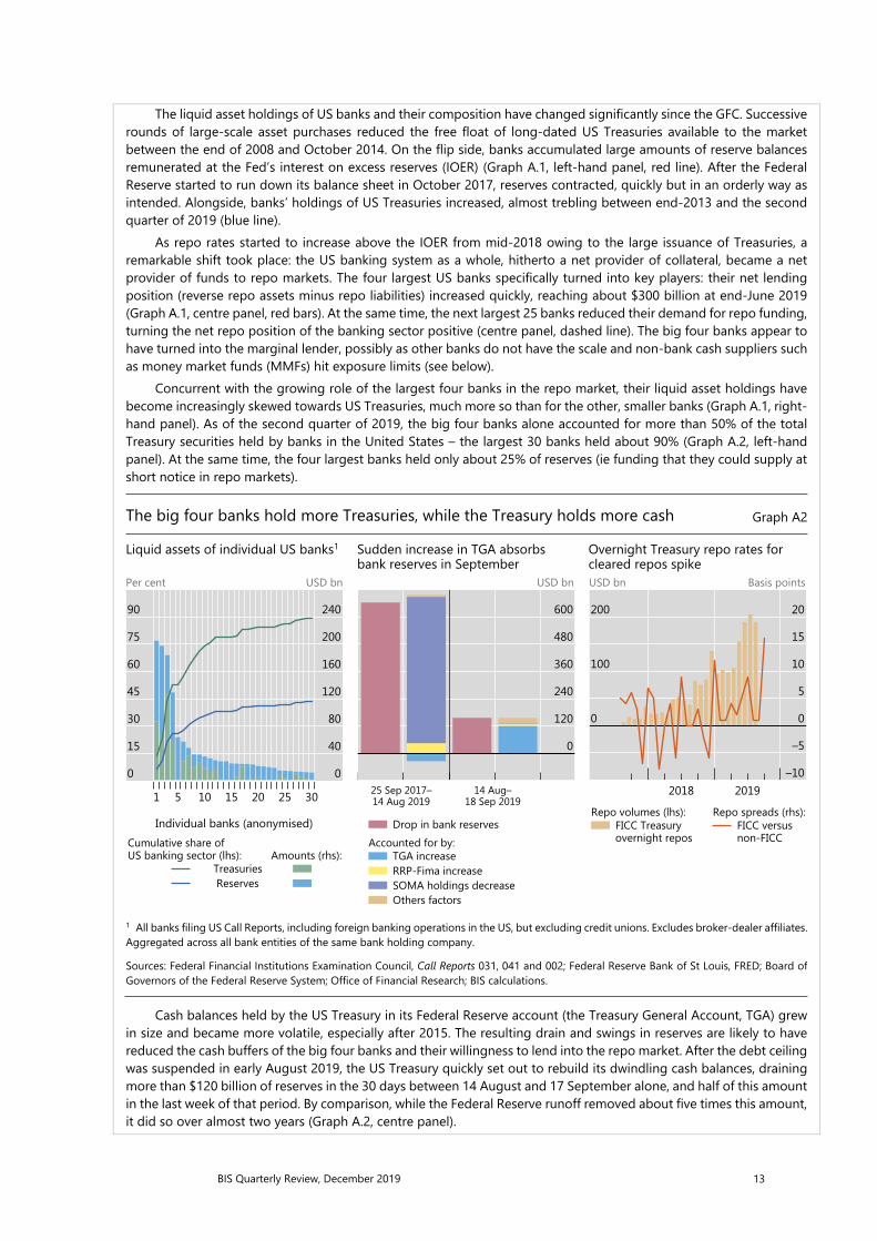
The liquid asset holdings of US banks and their composition have changed significantly since the GFC. Successive rounds of large-scale asset purchases reduced the free float of long-dated US Treasuries available to the market between the end of 2008 and October 2014. On the flip side, banks accumulated large amounts of reserve balances remunerated at the Fed’s interest on excess reserves (IOER) (Graph A.1, left-hand panel, red line). After the Federal Reserve started to run down its balance sheet in October 2017, reserves contracted, quickly but in an orderly way as intended. Alongside, banks’ holdings of US Treasuries increased, almost trebling between end-2013 and the second quarter of 2019 (blue line).
As repo rates started to increase above the IOER from mid-2018 owing to the large issuance of Treasuries, a remarkable shift took place: the US banking system as a whole, hitherto a net provider of collateral, became a net provider of funds to repo markets. The four largest US banks specifically turned into key players: their net lending position (reverse repo assets minus repo liabilities) increased quickly, reaching about $300 billion at end-June 2019 (Graph A.1, centre panel, red bars). At the same time, the next largest 25 banks reduced their demand for repo funding, turning the net repo position of the banking sector positive (centre panel, dashed line). The big four banks appear to have turned into the marginal lender, possibly as other banks do not have the scale and non-bank cash suppliers such as money market funds (MMFs) hit exposure limits (see below).
Concurrent with the growing role of the largest four banks in the repo market, their liquid asset holdings have become increasingly skewed towards US Treasuries, much more so than for the other, smaller banks (Graph A.1, right-hand panel). As of the second quarter of 2019, the big four banks alone accounted for more than 50% of the total Treasury securities held by banks in the United States – the largest 30 banks held about 90% (Graph A.2, left-hand panel). At the same time, the four largest banks held only about 25% of reserves (ie funding that they could supply at short notice in repo markets).
The big four banks hold more Treasuries, while the Treasury holds more cash Graph A2
Liquid assets of individual US banks1 Sudden increase in TGA absorbs bank reserves in September
Overnight Treasury repo rates for cleared repos spike
Per cent USD bn USD bn USD bn Basis points
1 All banks filing US Call Reports, including foreign banking operations in the US, but excluding credit unions. Excludes broker-dealer affiliates. Aggregated across all bank entities of the same bank holding company. Sources: Federal Financial Institutions Examination Council, Call Reports 031, 041 and 002; Federal Reserve Bank of St Louis, FRED; Board of Governors of the Federal Reserve System; Office of Financial Research; BIS calculations.
Cash balances held by the US Treasury in its Federal Reserve account (the Treasury General Account, TGA) grew in size and became more volatile, especially after 2015. The resulting drain and swings in reserves are likely to have reduced the cash buffers of the big four banks and their willingness to lend into the repo market. After the debt ceiling was suspended in early August 2019, the US Treasury quickly set out to rebuild its dwindling cash balances, draining more than $120 billion of reserves in the 30 days between 14 August and 17 September alone, and half of this amount in the last week of that period. By comparison, while the Federal Reserve runoff removed about five times this amount, it did so over almost two years (Graph A.2, centre panel).
90
75
60
45
30
15
0
240
200
160
120
80
40
0
302520151051
Treasuries Reserves
US banking sector (lhs):Cumulative share of
Amounts (rhs):
Individual banks (anonymised)
600
480
360
240
120
0
18 Sep 201914 Aug 201914 Aug–25 Sep 2017–
Drop in bank reserves
TGA increaseRRP-Fima increaseSOMA holdings decreaseOthers factors
Accounted for by:
200
100
0
20
15
10
5
0
–5
–1020192018
overnight reposFICC Treasury
Repo volumes (lhs):
non-FICCFICC versus
Repo spreads (rhs):

14 BIS Quarterly Review, December 2019
Besides these shifts in market structure and balance sheet composition, other factors may help to explain why banks did not lend into the repo market, despite attractive profit opportunities. A reduction in money market activity is a natural by-product of central bank balance sheet expansion. If it persists for a prolonged period, it may result in hysteresis effects that hamper market functioning. For instance, the internal processes and knowledge that banks need to ensure prompt and smooth market operations may start to decay. This could take the form of staff inexperience and fewer market-makers, slowing internal processes. Moreover, for regulatory requirements – the liquidity coverage ratio – reserves and Treasuries are high-quality liquid assets (HQLA) of equivalent standing. But in practice, especially when managing internal intraday liquidity needs, banks prefer to keep reserves for their superior availability.
Shifts in repo borrowing and lending by non-bank participants may have also played a role in the repo rate spike. Market commentary suggests that, in preceding quarters, leveraged players (eg hedge funds) were increasing their demand for Treasury repos to fund arbitrage trades between cash bonds and derivatives. Since 2017, MMFs have been lending to a broader range of repo counterparties, including hedge funds, potentially obtaining higher returns. These transactions are cleared by the Fixed Income Clearing Corporation (FICC), with a dealer sponsor (usually a bank or broker-dealer) taking on the credit risk. The resulting remarkable rise in FICC-cleared repos indirectly connected these players. During September, however, quantities dropped and rates rose, suggesting a reluctance, also on the part of MMFs, to lend into these markets (Graph A.2, right-hand panel). Market intelligence suggests MMFs were concerned by potential large redemptions given strong prior inflows. Counterparty exposure limits may have contributed to the drop in quantities, as these repos now account for almost 20% of the total provided by MMFs.
Since 17 September, the Federal Reserve has taken various measures to supply more reserves and alleviate repo market pressures. These operations were expanded in scope to term repos (of two to six weeks) and increased in size and time horizon (at least through January 2020). The Federal Reserve further announced on 11 October the purchase of Treasury bills at an initial pace of $60 billion per month to offset the increase in non-reserve liabilities (eg the TGA). These ongoing operations have calmed markets. On the same day, the effective federal funds rate increased only 5 basis points to 2.30% (above the upper limit of the federal funds target), but the intraday range spiked to almost 200 basis points, from a typical range of less than 10 basis points. J Williams, “Money markets and the federal funds rate: the path forward”, speech 332, Federal Reserve Bank of New York, 17 October 2019. Concerns about market functioning due to depressed interbank trading activity in an abundant reserves regime were an important consideration behind the Central Bank of Norway’s switch to a quota-based system in 2011. Markets Committee, Large central bank balance sheets and market functioning, October 2019. See I Aldasoro, T Ehlers and E Eren, ”Can CCPs reduce repo market inefficiencies?”, BIS Quarterly Review, December 2017, pp 13–14. On 18–20 September, it offered overnight repos to primary dealers of up to an aggregate amount of $75 billion against Treasury, agency debt and agency mortgage-backed securities collateral. From 15 November, at least $120 billion in daily overnight repos, in addition to at least $35 billion in two-week term repos, was offered twice a week and at least $15 billion for four- or six-week repos was offered weekly.
BIS Quarterly Review, December 2019 15
FX and OTC derivatives markets through the lens of the Triennial Survey1
The 2019 BIS Triennial Central Bank Survey provided new insights about the boost that electronification gave to trading in FX and OTC derivatives markets, and the role of compression and clearing in containing the growth of outstanding derivatives exposures. JEL classification: F31, G15, G23
This special issue of the BIS Quarterly Review analyses the results of the latest BIS Triennial Central Bank Survey of Foreign Exchange and Over-the-counter (OTC) Derivatives Markets (Triennial Survey). The collection of five articles explores what factors drove the recent growth of these markets and what those factors tell us about the evolution of the markets’ structure. The message that emerges is that OTC markets are larger and more diversified than ever, owing in part to the rise of electronic and automated trading. Even as trading picked up, compression and clearing helped to contain the growth of outstanding derivatives exposures.
The Triennial Survey is the most comprehensive source of information on the size and structure of foreign exchange (FX) and OTC derivatives markets. The BIS coordinates it in cooperation with central banks worldwide under the guidance of the Markets Committee and the Committee on the Global Financial System. The survey has been conducted every three years since 1986. In 2019, almost 1,300 dealers (mainly banks) located in 53 countries participated. Data were collected in two stages: OTC trading of FX spot, FX derivatives and interest rate derivatives was surveyed in April 2019, and the outstanding notional amounts and gross market values of all OTC derivatives were surveyed at the end of June.2
Offshore markets propel trading growth
FX and OTC derivatives markets saw a marked pickup in trading between the 2016 and 2019 surveys. Following a dip in 2016, FX trading returned to its long-term
1 The views expressed in this article are those of the author and do not necessarily reflect those of the
Bank for International Settlements. 2 For more information about the Triennial Survey and to explore the data, see
www.bis.org/statistics/rpfx19.htm.
Philip [email protected]

16 BIS Quarterly Review, December 2019
upward trend, rising to $6.6 trillion per day in April 2019. Interest rate derivatives trading departed sharply from its previous trend, soaring to $6.5 trillion.
The trading of short-term instruments grew faster than that of long-term instruments. This mechanically increased reported turnover because such contracts need to be replaced more often. Schrimpf and Sushko (2019a) emphasise that the trading of FX swaps, which is concentrated in maturities of less than a week, rose from $2.4 trillion in April 2016 to $3.2 trillion in April 2019 and accounted for most of the overall increase in FX trading. In interest rate derivatives markets historically, OTC contracts had mainly referenced long-term rates; contracts referencing short-term rates were traded on exchanges. Using overnight index swaps and forward rate agreements as a proxy for OTC derivatives referencing short-term interest rates, Ehlers and Hardy (2019) find that OTC trading of such derivatives probably surpassed that of derivatives on long-term rates in April 2019.
While globally trading continued to be dominated by the major currencies, in particular the US dollar and the euro, in FX markets the trading of emerging market currencies grew faster than that of major currencies. As discussed by Patel and Xia (2019), the share of emerging market currencies in global FX turnover rose to 23% in April 2019 from 19% in 2016 and 15% in 2013. In contrast, interest rate derivatives denominated in emerging market currencies saw their share of global activity decline. Aramonte and Huang (2019) highlight that the OTC derivatives exposures of dealers headquartered in emerging market economies were concentrated in FX instruments, whereas those of dealers from advanced economies were concentrated in interest rate instruments.
The pickup in turnover between 2016 and 2019 was especially marked in offshore markets. Trading tended to grow most for those currencies with greater increases in activity offshore than onshore. The Chinese renminbi illustrates this: subdued growth coincided with a decline in the share of offshore trading. The renminbi’s rank as the eighth most traded currency was unchanged between 2016 and 2019 and, according to Packer et al (2019), turnover remained lower than expected, based on trade and GDP per capita.
Greater offshore trading went hand in hand with greater geographical concentration. In FX markets, London, New York, Singapore and Hong Kong SAR increased their collective share of global trading to 75% in April 2019, up from 71% in 2016 and 65% in 2010. Trading in OTC interest rate derivatives markets was also increasingly concentrated in a few financial centres, especially London. Schrimpf and Sushko (2019a) attribute this geographical concentration to network externalities. For example, it is more cost-effective to centralise counterparty and credit relationships, or technical and legal infrastructures, in a handful of hubs than to spread them across many countries. The faster pace of trading also increased the advantages of locating traders’ IT systems physically close to those of the platforms on which they trade.
Even as trading became more concentrated geographically, it fragmented across platforms. Schrimpf and Sushko (2019b) explain how the distinction in FX markets
Key takeaways
• The 2019 BIS Triennial Central Bank Survey showed that FX and OTC derivatives markets were larger and more diversified than ever.
• Electronification propelled the growth of offshore trading and increased the diversity of market participants. • In FX markets, the rise in trading was led by swaps, while settlement risk remains a major concern.

BIS Quarterly Review, December 2019 17
between the inter-dealer and dealer-customer segments is increasingly blurred. Principal trading firms (PTFs),3 in particular, made inroads into market-making activities, and the ways in which customers could conduct trades proliferated.
Electronification is reshaping markets
Turning to what factors drove the recent growth of FX and OTC derivatives markets, one stood out: the rise in electronic and automated trading, also referred to as electronification. By reducing transaction costs, electronification has boosted trading and changed price formation and liquidity provision. FX spot was one of the first OTC markets to go electronic, and the FX forwards market is quickly catching up, especially the market for non-deliverable FX forwards (NDFs). In contrast, as Schrimpf and Sushko (2019b) point out, the electronification of FX swaps lags because of their large size, complex pricing and the credit risk involved. OTC interest rate derivatives markets, too, are shifting from voice brokers to electronic platforms. Ehlers and Hardy (2019) cite electronification as a key reason for the faster growth of OTC trading relative to exchange trading of interest rate derivatives.
Another notable driver of growth was the increased diversity of market participants. Greater heterogeneity in participants’ transaction needs and investment horizons has enhanced market liquidity and facilitated risk transfers. To some extent, greater diversity was linked to electronification. Electronification has enabled automated trading, in particular high-frequency trading. This, in turn, has made OTC markets more attractive to those engaged in such strategies, mainly hedge funds and PTFs.
The market for NDFs shows how electronification has stimulated trading and increased the diversity of market participants. Currencies that are not freely convertible were among those recording the fastest growth in FX turnover between the 2016 and 2019 surveys, including the Indian rupee, Indonesian rupiah and Philippine peso. Patel and Xia (2019) highlight that this growth was led by forwards, particularly NDFs traded in offshore markets.
Changes in the size, investment objectives and strategies of asset managers have also served to increase the diversity of OTC market participants. Since the Great Financial Crisis (GFC) of 2007–09, assets managed by investment funds, exchange-traded funds and other non-bank investors have expanded substantially. At the same time, low interest rates have encouraged riskier investments. According to Patel and Xia (2019), this has raised non-bank financial institutions’ demand for emerging market assets. Similarly, Ehlers and Hardy (2019) emphasise that non-bank financial institutions have made more active use of OTC interest rate derivatives.
In addition to such market-wide structural changes, other factors have contributed to the growth of specific market segments. As Schrimpf and Sushko (2019a) explain, trading in FX swaps was boosted by banks’ liquidity management as well as their arbitraging of interest rate differentials for funding in different currencies. Another driver of FX trading was the recovery in prime brokerage activities4 from the 3 PTFs are firms that invest, hedge or speculate for their own account. PTFs include high-frequency
trading firms as well as electronic non-bank market-makers. 4 Prime brokerage refers to intermediation services that dealers provide to hedge funds, PTFs and
other selected customers. Prime brokers are usually large highly rated banks. They enable selected

18 BIS Quarterly Review, December 2019
subdued levels of 2016, when losses on clients’ trades following idiosyncratic events in FX markets had caused some banks to retrench. For OTC interest rate derivatives, Ehlers and Hardy (2019) highlight how changes in the level and volatility of US dollar interest rates boosted turnover in April 2019.
Compression and clearing mitigate exposures
The marked pickup in the trading of FX and OTC derivatives between the 2016 and 2019 surveys did not lead to an increase in outstanding exposures. To be sure, since 2015 the notional principal of outstanding OTC derivatives has trended upwards, and at end-June 2019 it reached its highest level since 2014. However, their gross market value – a more meaningful measure of amounts at risk than notional principal – has trended downward since 2012. As Aramonte and Huang (2019) highlight, the gross market value was $12 trillion at end-June 2019, close to its level immediately before the GFC.
Compression and clearing helped to slow the growth of outstanding exposures. Compression eliminates economically redundant derivatives positions and thereby reduces outstanding contracts. Compression first took hold in the market for credit default swaps (CDS), where even before the GFC it contributed to a sharp reduction in notional principal. While it took longer to penetrate OTC interest rate derivatives markets, Ehlers and Hardy (2019) document that the frequency and amount of compression has increased in recent years, making it now commonplace. Compression, coupled with electronification and other changes, is reshaping OTC markets along the lines of exchanges.
Compression has been greatly facilitated by the expansion of central clearing. Clearing rates for CDS and OTC interest rate derivatives rose steadily between 2010 and 2017, though they have since levelled off. By 2019, derivatives subject to mandatory clearing, mainly forward rate agreements, interest rate swaps and CDS indices, were almost all centrally cleared. Aramonte and Huang (2019) find that, among derivatives not subject to mandatory clearing, some have migrated to central clearing voluntarily. The decision whether to migrate contracts depends on the benefits of lower margin requirements, potential gains from netting positions within the same asset class and relative liquidity conditions.
In contrast to trends in other segments of OTC markets, in FX markets initiatives to mitigate risk exposures appear to have stalled. Most FX instruments are deliverable contracts, which involve an exchange of principal. Thus, settlement risk – the risk that one counterparty fails to deliver after the other has delivered – is a major concern. In the 2000s, a number of initiatives, most notably the establishment of Continuous Linked Settlement, a specialist institution that settles FX transactions on a payment-versus-payment basis, led to a big reduction in FX settlement risk. However, Bech and Holden (2019) conclude that FX settlement risk has risen since 2013. In particular, the proportion of trades using payment-versus-payment systems has declined. Encouraging use of these systems and opening them to fast-growing emerging market currencies would help to reverse this trend.
customers to conduct trades, subject to credit limits, with a group of predetermined counterparties in the prime broker’s name.

BIS Quarterly Review, December 2019 19
References
Aramonte, S and W Huang (2019): “OTC derivatives: euro exposures rise and central clearing advances”, BIS Quarterly Review, December, pp 83–93. Bech, M and H Holden (2019): “FX settlement risk remains significant”, BIS Quarterly Review, December, pp 48–49. Ehlers, T and B Hardy (2019): “The evolution of OTC interest rate derivatives markets”, BIS Quarterly Review, December, pp 69–82. Packer, F, A Schrimpf and V Sushko (2019): “Renminbi turnover tilts onshore”, BIS Quarterly Review, December, pp 35–6. Patel, N and D Xia (2019): “Offshore markets drive trading in emerging market currencies”, BIS Quarterly Review, pp 53–67. Schrimpf, A and V Sushko (2019a): “Sizing up global foreign exchange markets”, BIS Quarterly Review, December pp 21–38. ——— (2019b): “FX trade execution: highly complex and fragmented”, BIS Quarterly Review, December, pp 39–51.

BIS Quarterly Review, December 2019 21
Sizing up global foreign exchange markets1
The latest BIS Triennial Survey shows that global foreign exchange trading increased to more than $6 trillion per day. Trading bounced back strongly following a dip in 2016, buoyed by increased trading with financial clients such as lower-tier banks, hedge funds and principal trading firms. Prime brokerage volumes recovered in tandem. These developments were driven in large part by the greater use of FX swaps for managing funding and greater electronification of customer trading. They led to further concentration of trading in a few financial hubs. JEL classification: C42, C82, F31, G12, G15.
Turnover in global foreign exchange (FX) markets reached $6.6 trillion per day in April 2019. This is up from $5.1 trillion per day in April 2016 and marked a return to the long-term upward trend in turnover recorded in each BIS Triennial Central Bank Survey since 2001. In this article, we explore the recent evolution in the size and structure of global FX markets by drawing on the latest survey.
The global FX market is more opaque than many other financial markets because it is organised as an over-the-counter (OTC) market built upon credit relationships. In recent years, changes in market structure, such as the internalisation of trades in dealers’ proprietary liquidity pools, further reduced the share of trading activity that is “visible” to other market participants (Schrimpf and Sushko (2019) in this issue). The Triennial Survey provides a comprehensive, albeit infrequent, snapshot of activity in this highly fragmented market.2
1 We thank Sirio Aramonte, Claudio Borio, Alain Chaboud, Ying-Wong Cheung, Stijn Claessens, Torsten
Ehlers, Ingo Fender, Brian Hardy, Wenqian Huang, Robert McCauley, Dagfinn Rime, Maik Schmeling, Olav Syrstad and Philip Wooldridge for helpful comments and suggestions. We also appreciate the feedback and insightful discussions with a number of market participants at major FX dealing banks, buy-side institutions, electronic market-makers and trading platform providers. We are also grateful to Yifan Ma and Denis Pêtre for compiling the data and Adam Cap for excellent research assistance. The views expressed are those of the authors and do not necessarily reflect those of the Bank for International Settlements.
2 Central banks and other authorities in 53 jurisdictions participated in the 2019 survey, which collected data from close to 1,300 banks and other dealers. For information about the Triennial Survey, see www.bis.org/statistics/rpfx19.htm.
Andreas [email protected]
Vladyslav [email protected]

22 BIS Quarterly Review, December 2019
FX trading volumes in April 2019 were buoyed by a pickup in trading with financial clients, such as smaller banks, hedge funds and principal trading firms (PTFs). FX prime brokerage – intermediation services provided by top-tier FX dealers to financial clients – recovered in tandem. Prime brokerage expanded across all instruments, but was particularly visible in spot trading. This was largely due to a more active presence of PTFs, some of which have gained a firm footing as non-bank electronic market-makers. It also offset the continued decline in spot trading in inter-dealer markets.
A pickup in trading of FX swaps, especially by smaller banks, was the largest single contributor to the overall FX turnover growth (Annex Table A1). It was mainly driven by the use of swaps in banks’ funding management. Another noteworthy development was robust trading in forwards, particularly in the non-deliverable forward (NDF) segment attractive to hedge funds and PTFs. While the increase in the trading of FX swaps and forwards accounted for about 75% of the rise in global FX volumes since 2016, growth in spot was more muted due to a prolonged period of subdued volatility and a decline in inter-dealer spot trading.
Electronification in FX first took off in inter-dealer trading, but its trajectory has since changed. In recent years, the dealer-to-customer segment has seen the strongest rise in electronification. To the extent that electronic trading tends to be booked in a few major financial hubs, it also leads to a greater share of offshore trading.
This article is organised as follows. The first section provides empirical evidence of financial drivers behind FX volumes. The second digs deeper into developments in FX swaps, with a particular focus on trading by banks. The third discusses broader trends in trading with financial clients and across instruments, as well as FX prime brokerage. The fourth takes stock of the degree of electronification in FX trading across key market segments. The fifth section focuses on the trend towards more concentration of trading in major FX hubs, and, by extension, increased offshore trading. The final section concludes.
FX trading volumes mostly reflect financial motives
The recovery in volumes recorded in the 2019 Triennial Survey follows some unusually subdued trading activity three years ago, when the survey had shown a decline for the first time since 2001 (Graph 1, left-hand panel). In 2016, the prime brokerage
Key takeaways
• Trading in global FX markets reached $6.6 trillion per day in April 2019, up from $5.1 trillion in April 2016. • Increased use of FX swaps for bank funding liquidity management and hedging of foreign currency
portfolios, as well as growth in prime brokerage, boosted trading. • Electronification of FX markets spurred an even greater concentration of trading in a few financial hubs.

BIS Quarterly Review, December 2019 23
business had still not fully recovered from the 2015 Swiss franc shock,3 the banking industry was adjusting to the new regulatory environment, and the composition of participants had changed in favour of more risk-averse players (Moore et al (2016)). Semiannual surveys by FX committees and other sources in the major centres confirm that 2019 represented a return to the long-term upward trend in FX trading (centre panel).4
The 2019 survey shows that the evolution of FX trading volumes continues to be dominated mostly by financial institutions’ motives as opposed to needs arising directly from real economic activity. The customer segment most closely linked to global trade is non-financial corporations, and in 2019 its share of trading remained almost unchanged at less than 8% (Graph 1, right-hand panel). The long-term shift towards financial customers outside the dealer community resumed, with the share of trading with other financial institutions rising from 51% in 2016 to 55% in 2019. By contrast, trading among reporting dealers grew little, so that the inter-dealer share in overall FX volumes continued its downward trend.
Regression analysis confirms the dominance of financial motives. As shown in Table 1, trade in goods and services shows a positive link with FX turnover (column 1),
3 The abandonment of the Swiss franc’s floor regime with the euro on 15 January 2015 led to extreme
currency moves. It shook the entire FX industry, especially prime brokerage, and exerted lasting effects on trading volumes (see Box A and Moore et al (2016)).
4 Global FX turnover probably briefly surpassed $6 trillion already in September 2014, as discussed in Box A in Moore at al (2016).
FX turnover rises with more trading in FX swaps and by financials Graph 1
FX turnover resumed upward trend1 FX committee and CFETS volumes2 Financial customers dominated1, 4 USD trn USD trn Per cent
1 Adjusted for local and cross-border inter-dealer double-counting, ie “net-net” basis; daily averages in April. 2 Semiannual data, referring to April and October. Additional increase in stacked bars due to the inclusion of China Foreign Exchange Trade System (CFETS) turnover in April 2015 and the Hong Kong Treasury Markets Association survey in April 2017. 3 The benchmarking using the proportional Denton technique allows us to assess the evolution of FX trading volumes between Triennial surveys. For a description, see Bech (2012). 4 Expressed as a share of total turnover. Sources: M Bech, “FX volume during the financial crisis and now”. BIS Quarterly Review. March 2012. pp 33–43; foreign exchange committee surveys; Bloomberg; BIS Triennial Central Bank Survey; authors’ calculations.
6
4
2
0
19161310070401
TotalSpotFX swaps
Outright forwardsOptionsCurrency swaps
6.0
4.8
3.6
2.4
1.2
0.0
20192017201520132011
Benchmarked series3
Triennial survey1
LondonNew YorkSingaporeHong Kong SAR
TokyoAustraliaCanadaCFETS
45
30
15
0
19161310070401
Reporting dealersNon-financial customersOther financial institutions

24 BIS Quarterly Review, December 2019
yet currencies featuring greater participation by corporates show sub-par growth (column 2). By contrast, FX turnover growth is better captured when financial flows (column 3) and the share of trading with financial clients (column 4) are accounted for. Furthermore, currencies featuring a higher share of trading offshore in financial centres have also seen higher FX turnover (column 5).5
Zooming in on FX swaps
Since 2013, FX swaps and forwards have been the main instruments behind the growth in overall FX trading (Graph 1, left-hand panel).6 Their combined share of turnover rose from 54% in 2013 to 61% in 2016, and 64% in 2019. By contrast, the share of spot trading fell from 38% to 30% over this period.
The share of the US dollar in swaps is even higher than in spot, with USD on one side in more than 90% of FX swap turnover. The three most traded FX swap crosses
5 These results extend the findings of McCauley and Scatigna (2011) and Chitu et al (2014). At the same
time, these results may understate the importance of corporate clients in affecting FX flow. While large multinational corporations may trade directly with top-tier FX banks (captured as such in the Triennial), other corporates are more likely to be intermediated by smaller and more locally oriented (non-reporting) banks. Trading by the latter could hence effectively act as a conduit for real economy driven flows to reach the FX market.
6 An FX swap is an OTC derivatives contract consisting of a spot and a forward leg. Effectively it is a term loan of one currency collateralised with another currency. While FX swaps constitute an off-balance sheet derivatives position from an accounting perspective, in many respects they fulfil a similar economic function to secured foreign currency debt (Borio et al (2017)). The pricing of the FX swap, ie the forward premium/discount, is linked to money market rates in the two currencies via a law of one price relation known as covered interest parity (CIP).
Drivers of FX trading growth Table 1
(1) (2) (3) (4) (5) Trade flows 0.16***
(0.03) 0.15*** (0.03)
0.09** (0.04)
0.08** (0.03)
0.07** (0.03)
Corporate clients –0.08** (0.03)
Financial flows 0.15*** (0.04)
0.16*** (0.03)
0.15*** (0.03)
Financial clients 0.13*** (0.04)
0.08** (0.04)
Offshore share
0.11*** (0.03)
Number of observations 194 188 154 151 151 R-squared 0.12 0.14 0.21 0.27 0.32 The following variables are specified as log differences: FX turnover (USD millions); trade flows = exports plus imports of goods and services (USD millions); corporate clients = share of non-financial counterparties in total turnover; financial flows = net acquisition of financial assets plus net incurrence of liabilities (USD millions). The following variables are specified as changes in integer percentage shares between surveys: financial clients = share of (non-dealer) financial counterparties; offshore share = share of offshore turnover (intra-euro area transactions are classified as offshore in the calculation of the EUR offshore share). Panel data for 26 individual currencies in five survey periods (2007, 2010, 2013, 2016 and 2019). Coefficients and standard errors scaled by the standard deviation of each variable in order to infer economic magnitudes; standard errors in brackets. ***/**/* indicates p-values less than 0.01/0.05/0.1, respectively. Constant not shown. Sources: IMF, Balance of Payments Statistics and World Economic Outlook; BIS Triennial Central Bank Survey; authors’ calculations.

BIS Quarterly Review, December 2019 25
are USD/EUR, USD/JPY and USD/GBP (Graph 2, left-hand panel). Two factors explain the dollar’s dominance. First, it is the international funding currency of choice, and second, it serves as the primary vehicle currency for trading FX instruments.
FX swap trading picked up significantly between 2016 and 2019 (Graph 2, centre panel). The market has been in the spotlight since about 2014 on the back of the resurgence in price “anomalies” (right-hand panel; Borio et al (2016), Du et al (2018)). The rise in FX swap volumes went hand in hand with the divergence of FX swap-implied funding costs from money market rates in the respective currencies, continuing a trend already observed in 2016 (Moore et al (2016)).
Banks dominate FX swap trading
Inter-dealer trading accounted for 47% of all FX swap turnover. FX dealers can trade swaps for their own banks’ treasury unit for funding, or on behalf of clients for funding and hedging purposes. They can also use FX swaps to construct offsetting hedges for their positions in related instruments, such as forwards and (longer-dated) currency swaps. Smaller banks (“non-reporting banks” in the survey terminology) accounted for another 30% of FX swap turnover. They enter FX swap transactions with reporting dealers to manage their own funding or FX hedging needs, or in order to provide intermediation services to their own local customer base, such as smaller and medium-sized corporates.7
7 Market sources indicate that second-tier banks have also increased their own presence as FX swap
intermediaries. Krohn and Sushko (2019) find evidence that smaller banks displaced larger dealers as market-makers in FX swaps at times when large banks managed down their balance sheets around regulatory reporting periods.
Trading in FX swaps boosted by trading with bank customers Graph 2
Benchmarked FX swap turnover1 FX swap trading by counterparty2 FX swap-implied currency basis3 USD trn USD trn Basis points
1 The vertical lines indicate April 2013, April 2016 and April 2019 (the dates of the BIS Triennial Survey). Benchmarked series are calculated using the proportional Denton technique. Based on breakdowns by currency pairs from the foreign exchange committees in London, New York, Singapore, Tokyo and Australia. The breakdown for USD/CHF and USD/CAD is not available from the Tokyo foreign exchangecommittee. 2 Adjusted for local and cross-border inter-dealer double-counting, ie “net-net” basis; daily averages in April. 3 Difference between FX swap-implied US dollar three-month interest rate and US dollar three-month Libor. Negative values indicate that FX swap-implied US dollar rate exceeds US dollar Libor and vice versa. Sources: Foreign exchange committee surveys; Bloomberg; BIS Triennial Central Bank Survey; authors’ calculations.
3
2
1
019181716151413
TotalEURJPYGBPAUD
USD vis-à-vis:CHFCADOther
49% 51%47%
27% 24%
30% 7% 12%
7%
13%11%
13% 3
2
1
0201920162013
Reporting dealersNon-reporting banksInstitutional investorsHedge funds and PTFsOther
0
–30
–60
–9019181716151413
EURJPYAUD
Three-month basis, USD vis-à-vis:

26 BIS Quarterly Review, December 2019
Funding liquidity management and hedging of FX assets
The renewed expansion in FX swaps in the 2016–19 period largely owed to the increasing participation of lower-tier banks. The trading of these smaller and regional banks outside the group of global FX dealers accounted for $404 billion (about half) of the total increase in swap turnover. These banks relied more heavily on FX swaps for funding because they have more limited direct access to US dollar funding.
Major central banks’ divergent balance sheet policies also affected banks’ incentives to trade in FX swap markets. For instance, the abundant liquidity in the euro area strengthened European banks’ incentives to swap excess euro liquidity into US dollars. Market sources indicate that this was driven by the demand to place abundant euro cash into a dollar-denominated safe and liquid asset, even if that meant paying up in the FX swap market to convert the currency. The actual need to fund longer-term dollar-denominated assets, by contrast, was reportedly a lesser consideration.
Banks’ use of FX swaps for managing funding liquidity naturally favours shorter-term tenors. Indeed, $2.1 trillion, or 64%, of FX swap turnover was in maturities of seven days or less (Graph 3, left-hand panel). Over the 2016–19 period, the use of FX swaps relative to on-balance sheet funding by foreign bank affiliates in the US increased significantly (centre panel). This points to the importance of FX swaps in banks’ funding liquidity management.
At the same time, asset managers and other investors also rely on FX swaps as rolling hedges for currency risk in international bond portfolios and passive investment fund vehicles. These have grown in both amounts and duration in recent
Maturity profile of FX swaps and importance for funding and hedging Graph 3
FX swap turnover by maturity1 FX swaps and forwards reported by US branches of non-US banks3
Institutional investor FX swap trading and FX-hedged US dollar yields
USD bn USD bn Ratio USD bn Per cent
1 Adjusted for local and cross-border inter-dealer double-counting, ie “net-net” basis; daily averages in April. 2 Predicted distribution based on the assumption of an inverse relationship between turnover and maturity; using discrete maturities of one week, one month, three months, six months and one year for each maturity bucket; for example, daily turnover of one-week FX swaps is assumed to be four times that of one-month ones, daily turnover of one-month FX swaps is assumed to be three times that of three-month ones, etc. 3 Based on Federal Financial Institutions Examination Council, Report of Assets and Liabilities of US Branches and Agencies of Foreign Banks using Q1 data. 4 Calculated as the gross notional divided by total on-balance sheet liabilities. 5 Ten-year US Treasury yields adjusted for FX hedging cost by subtracting the forward premium of the respective currency pair. Sources: US Federal Financial Institutions Examination Council; Bloomberg; BIS Triennial Central Bank Survey; authors’ calculations.
2,000
1,500
1,000
500
0
Up to
a w
eek
8 da
ys–1
mon
th1–
3 m
onth
s3–
6 m
onth
sOv
er 6
mon
ths
Actual Predicted2
400
300
200
100
0
0.20
0.15
0.10
0.05
0.002019201620192016
FX swaps Forwards
(lhs): Notionals
Balance sheet ratio (rhs):4
120
80
40
0
6
4
2
0
–2201920162013
USD/EURUSD/JPY
Turnover (lhs):1
EURJPY
10-yr US yields hedged into (rhs):5

BIS Quarterly Review, December 2019 27
years. FX swaps of one- to three-month tenors, which were popular maturities for such hedges, thus saw higher turnover compared with what one would expect solely on the basis of the inverse relationship between instrument maturity and trading frequency.
Opportunistic behaviour: arbitrage trades
Banks can also use FX swaps in order to exploit the pricing differentials implicit in them (the “cross-currency basis”), by varying their short-term borrowing and/or placement of funds across currencies. Specifically, financial institutions endowed with large amounts of US dollar reserve balances, or those with cheaper access to direct sources of dollar funding as well as access to central bank deposit facilities in different currencies, have been in a position to arbitrage dislocations in short-dated FX swaps (Rime et al (2017)). Opportunistic behaviour tends to intensify around regulatory reporting dates, and it goes both ways. Dealers of some of the largest banks reduce their FX swap intermediation around these dates (Krohn and Sushko (2019)), while some non-US banks face incentives to actively manage down their on-balance sheet funding by switching to off-balance sheet instruments, such as FX swaps. By contrast, others can take advantage of pricing dislocations by taking the other side and supplying the sought-after currency via FX swaps. Some central banks are also active in FX swaps, mostly as lenders of their US dollar reserves.
Other forms of arbitrage can also make use of FX swaps. For example, the linked exchange rate system of HKD/USD operates by capital flows arbitraging fluctuations in the Libor-Hibor interest rate differential (HKMA (2018)). Higher interest rate volatilities and divergence from US rates over the past three years have induced more arbitrage flows, with investors using FX swaps to synthetically create long/short positions in money markets in the two currencies. Such activity explains a good part of the doubling of HKD/USD turnover since the last Triennial Survey.
FX swap trading by institutional investors falls
In contrast to the increased FX swap trading by banks, trading by institutional investors has contracted since the last Triennial. This development was most visible in EUR/USD and JPY/USD – the two major crosses (Graph 3, right-hand panel). Institutional investors, such as insurance companies, typically use longer-dated FX swaps or forwards to hedge the currency risk of their foreign bond holdings.
The decline in swap trading by institutional investors in EUR/USD and JPY/USD since 2016 is explained by the evaporation of the pickup in yield from investing in long-term US Treasury bonds on an FX-hedged basis. In the past, with long-term yields compressed in conjunction with monetary easing by the ECB and the Bank of Japan, euro area and Japanese institutional investors sought higher yields by investing in US Treasury bonds. At the same time, they hedged the currency risk with FX swaps. A flattening of the yield curve since late 2016 made US Treasuries less attractive, once hedging costs (which are predicated on short-term rates in the two currencies) were factored in.8
8 The relative steepness of the US yield curve (vis-à-vis investors’ home country one) matters because
FX hedging costs depend on the level of short-term rates while the investment returns are predicated on the level of long-term yields. More precisely, euro area or Japanese institutions effectively pay the short-end yield differential (via the FX swap transaction) and earn the long-end yield differential.

28 BIS Quarterly Review, December 2019
Trading with financial clients and FX prime brokerage
Dealers’ trading with “other financial institutions” – a category that includes non-reporting banks, hedge funds and PTFs, institutional investors and official sector financial institutions – grew notably since 2016 by $1 trillion, to $3.6 trillion. As such, the share of this heterogeneous group of financial clients has reached 55% of global volumes. Non-reporting banks – typically smaller, regional banks that serve as clients of the large FX dealer banks – remained the largest counterparty category within “other financial institutions”, accounting for $1.6 trillion in daily turnover (Graph 4, left-hand panel). As described above, most of the FX trading activity by these smaller banks is in FX swaps.
Trading with hedge funds and PTFs also increased significantly, to almost $600 billion. Hedge funds trade a variety of instruments, including FX swaps, forwards and options, which support their multi-asset trading strategies. By contrast, PTFs’ algorithmic trading strategies employ instruments featuring a high degree of electronification, especially spot and, most recently, forwards.
Prime-brokered turnover recovers
Close to a third of trading by other financial institutions in 2019 was done via prime brokers, according to our estimates (see Box A). In a prime-brokered transaction, top FX dealers allow clients to trade directly in the bank’s name with their established counterparties, subject to credit limits.9
9 This way, the client gains access to the deep liquidity of electronic trading venues.
FX trading by smaller banks, hedge funds and principal trading firms Graph 4
Turnover with other financial institutions decomposed1
Prime-brokered turnover1,2 PTF spot electronic liquidity provision to clients
USD trn USD trn Per cent Count
1 Adjusted for local and cross-border inter-dealer double-counting, ie “net-net” basis; daily averages in April. 2 Reporting dealers who act as prime brokers report both trades to which they are a counterparty as a result of their client trading on a prime-brokered basis: the “give-up” trade with the executing dealer and the value of the trade with the client. 3 Number of PTFs in the Euromoney list of top 10 spotelectronic liquidity providers by market share. Sources: Euromoney Foreign Exchange Survey; BIS Triennial Central Bank Survey; authors’ calculations.
2.0
1.5
1.0
0.5
0.02019201620192016
banksNon-reporting
and PTFsHedge funds
SpotFX swapsOutright forwards
1.2
0.9
0.6
0.3
0.020192016
OptionsCurrency swaps
40
30
20
10
0
4
3
2
1
02019201820172016
PTF spot e-trading market share (lhs)Number of PTFs in the top 10 (rhs)3

BIS Quarterly Review, December 2019 29
Fuelled by greater demand from non-bank financial clients, the prime brokerage industry has largely recovered since 2015–16. Prime-brokered turnover rose to $1.5 trillion in April 2019, a 68% increase compared with the 2016 survey. While the growth mostly took place in spot (Graph 4, centre panel), it also exhibited a fairly large increase in FX swaps, outright forwards and options. At the same time, more conservative prime broker business models, tighter risk management practices and know-your-customer rules have favoured retaining only larger clients.
Non-bank electronic market-makers spur spot volumes
The 2019 Triennial points to an increased footprint of the so-called “non-bank electronic market-maker” community, which forms part of the broader group of PTFs. PTFs in general thrive on fast, algorithmic strategies and rely on speed instead of balance sheet to trade large volumes.10 To gain access to the FX market, PTFs rely exclusively on prime brokers. The OTC FX trading activity by these firms is almost exclusively in spot and has contributed to the rise in spot turnover.
The broader set of PTFs has long engaged in both “aggressive” (initiating trades) and “passive” (serving as a willing counterparty to trades initiated by others) trading on anonymous electronic brokerage platforms. Passive trading effectively represents liquidity provision: it involves posting price quotes (limit orders) that can be hit by aggressive orders by a counterparty seeking to execute a trade at the prevailing market price. Yet the anonymity of such trading means that the counterparty does not know that it is trading with a PTF, nor can it count on being matched with the same liquidity provider in the future.
What sets non-bank electronic market-makers apart from their other PTF peers is the greater use of passive (ie liquidity-providing) strategies and disclosed liquidity provision via a network of client relationships. Not only does the counterparty on the other side, such as a smaller bank or an asset manager, know they are trading with a non-bank market-maker, but they also count on the same firm for their FX liquidity needs in the future as repeat customers.
Non-bank electronic market-makers have now penetrated deeply into the realm that, until about five years ago, was exclusive to bank dealers. The 2019 Euromoney survey indicates that the share of PTFs in spot e-trading with buy-side clients rose sharply to 32%, up from 10% three years earlier (Graph 4, right-hand panel).11 What differentiates these new players from traditional bank dealers is that they substitute speed for balance sheet. As they have morphed into market-makers, alongside main FX dealing banks, they have become an integral part of FX intermediation and a key determinant of liquidity conditions, particularly in the spot market.
10 In addition to market-making, PTF trading strategies can also include statistical arbitrage, latency
arbitrage and momentum or trend-following. Many PTFs have their roots as high-frequency trading firms in equity and futures markets, but then ventured into OTC trading in deep and liquid FX spot markets. Electronic prime brokerage offers them access and anonymity for executing high-speed algorithmic strategies on electronic venues.
11 The 2019 Euromoney rankings of top electronic spot liquidity providers include non-bank names such as XTX Markets, HC Tech, Jump Trading and Citadel Securities, alongside known bank dealers such as Deutsche Bank, JPMorgan, UBS, Citi, Goldman Sachs and Bank of America Merrill Lynch. Other PTFs with sizeable FX market footprints, many of which operate across other asset classes, include Flow Traders, GTS, Hudson Trading, Tower Research Capital and Virtu Financial.

30 BIS Quarterly Review, December 2019
Box A
FX prime brokerage and its contribution to trading volumes The biggest FX dealers in terms of volumes are also the biggest suppliers of prime brokerage (PB) services. PB enables clients to conduct trades with a group of predetermined third-party wholesale counterparties in the prime broker’s name and using the prime broker’s credit. This may also entail granting the client access to electronic platforms that once had been available only to major banks. By opening up the market and allowing greater participation by non-banks, PB has been an important catalyst of the move away from a clearly delineated two-tier market structure where dealers used to enjoy an exclusive role at the core.
FX prime brokerage Graph A1
Dealers who act as prime brokers (D3) allow some of their customers (C) to trade with a set of third-party banks (eg executing dealer D4) inthe prime broker’s name and using the prime broker’s credit lines. Source: BIS elaboration.
In an FX PB relationship, the prime broker (D3/PB) guarantees the payment to the counterparty to the client’s trade. As illustrated in Graph A1, the client (C) is granted credit to execute directly with another FX dealer (D4) in the prime broker’s name (D3/PB). Upon execution, the client trade is normally “given up” to the prime broker. When the prime broker is informed and accepts the transaction between its client and another wholesale market participant (ie the so-called executing dealer, D4), it is the prime broker (rather than the client) which becomes the party to the transaction. The transaction between the prime broker and the executing dealer is defined by what is called a “give-up agreement”.
A key benefit that prime brokers provide to their customers is anonymity: the counterparty to the customer’s trade (executing dealer D4) typically does not know that they are in fact dealing with a client (C) of a prime broker (dashed red arrow), as they only see the prime broker’s identity (D3/PB). Prime brokers receive a fee for these services, which also include consolidated settlement, clearing and reporting.
In 2019, close to a third of turnover with financial customers was prime-brokered, as estimated from the corresponding breakdown in the Triennial Survey (Graph A2, left-hand and centre panels). The rising prevalence of PB has implications for the turnover figures recorded by the Triennial. Even though effectively C trades with D4, there are actually two trades taking place which need to be recorded in the survey. In a scenario where two prime-brokered clients face each other directly, and their respective prime brokers each record another trade with their prime-brokered customer, a give-up trade executed by the two prime-brokered customers could create three times the turnover of a direct transaction. Hence, FX PB volumes to financial customers, which capture the amount of credit backing prime-
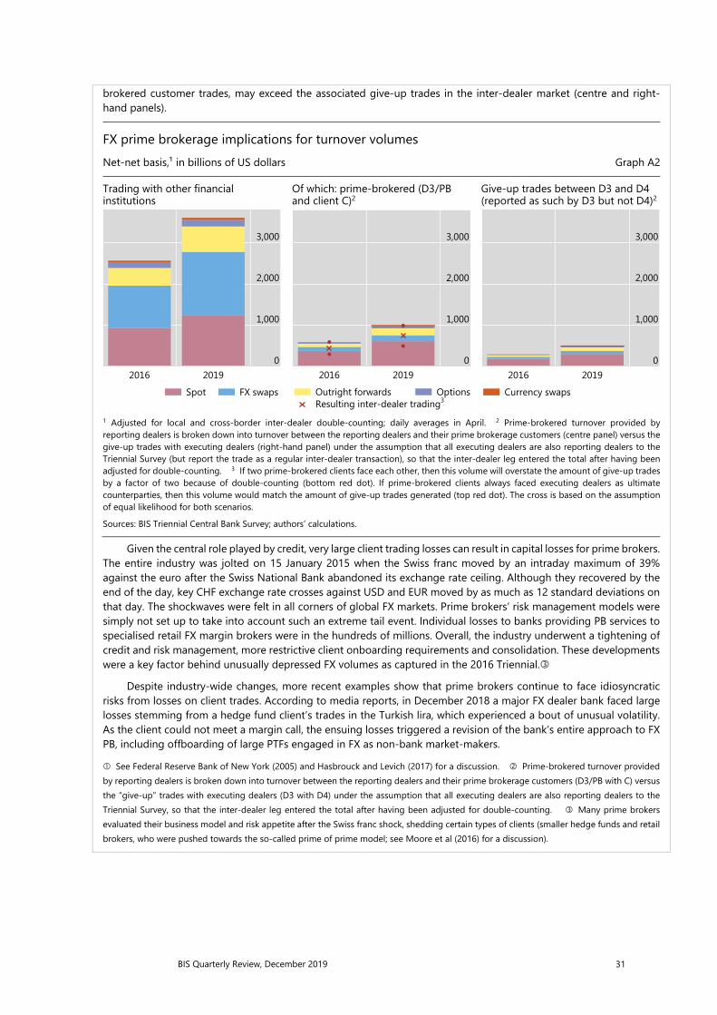
BIS Quarterly Review, December 2019 31
brokered customer trades, may exceed the associated give-up trades in the inter-dealer market (centre and right-hand panels).
FX prime brokerage implications for turnover volumes Net-net basis,¹ in billions of US dollars Graph A2
Trading with other financial institutions
Of which: prime-brokered (D3/PB and client C)2
Give-up trades between D3 and D4 (reported as such by D3 but not D4)2
1 Adjusted for local and cross-border inter-dealer double-counting; daily averages in April. 2 Prime-brokered turnover provided by reporting dealers is broken down into turnover between the reporting dealers and their prime brokerage customers (centre panel) versus the give-up trades with executing dealers (right-hand panel) under the assumption that all executing dealers are also reporting dealers to the Triennial Survey (but report the trade as a regular inter-dealer transaction), so that the inter-dealer leg entered the total after having beenadjusted for double-counting. 3 If two prime-brokered clients face each other, then this volume will overstate the amount of give-up trades by a factor of two because of double-counting (bottom red dot). If prime-brokered clients always faced executing dealers as ultimatecounterparties, then this volume would match the amount of give-up trades generated (top red dot). The cross is based on the assumptionof equal likelihood for both scenarios. Sources: BIS Triennial Central Bank Survey; authors’ calculations.
Given the central role played by credit, very large client trading losses can result in capital losses for prime brokers. The entire industry was jolted on 15 January 2015 when the Swiss franc moved by an intraday maximum of 39% against the euro after the Swiss National Bank abandoned its exchange rate ceiling. Although they recovered by the end of the day, key CHF exchange rate crosses against USD and EUR moved by as much as 12 standard deviations on that day. The shockwaves were felt in all corners of global FX markets. Prime brokers’ risk management models were simply not set up to take into account such an extreme tail event. Individual losses to banks providing PB services to specialised retail FX margin brokers were in the hundreds of millions. Overall, the industry underwent a tightening of credit and risk management, more restrictive client onboarding requirements and consolidation. These developments were a key factor behind unusually depressed FX volumes as captured in the 2016 Triennial.
Despite industry-wide changes, more recent examples show that prime brokers continue to face idiosyncratic risks from losses on client trades. According to media reports, in December 2018 a major FX dealer bank faced large losses stemming from a hedge fund client’s trades in the Turkish lira, which experienced a bout of unusual volatility. As the client could not meet a margin call, the ensuing losses triggered a revision of the bank’s entire approach to FX PB, including offboarding of large PTFs engaged in FX as non-bank market-makers. See Federal Reserve Bank of New York (2005) and Hasbrouck and Levich (2017) for a discussion. Prime-brokered turnover provided by reporting dealers is broken down into turnover between the reporting dealers and their prime brokerage customers (D3/PB with C) versus the “give-up” trades with executing dealers (D3 with D4) under the assumption that all executing dealers are also reporting dealers to the Triennial Survey, so that the inter-dealer leg entered the total after having been adjusted for double-counting. Many prime brokers evaluated their business model and risk appetite after the Swiss franc shock, shedding certain types of clients (smaller hedge funds and retail brokers, who were pushed towards the so-called prime of prime model; see Moore et al (2016) for a discussion).
3,000
2,000
1,000
020192016
Spot FX swaps
3,000
2,000
1,000
020192016
Outright forwardsResulting inter-dealer trading3
Options
3,000
2,000
1,000
020192016
Currency swaps

32 BIS Quarterly Review, December 2019
Electronification of trading across key market segments Electronic execution (e-trading) allows for fast trading and therefore contributes to overall FX turnover growth. In aggregate, the share of FX trading done electronically edged up only slightly to 56% in 2019. However, there are notable differences in the progress of electronification across instruments, and in inter-dealer versus dealer-to-customer market segments.
FX market electronification originally took off in the inter-dealer spot segment with the advent of centralised limit order books on electronic brokerage platforms such as EBS and Reuters (Refinitiv). However, this market segment no longer leads in electronification of FX trading. In fact, the share of e-trading in inter-dealer spot markets actually witnessed a decline (see Schrimpf and Sushko (2019) in this issue). It grew at a much faster pace in dealer-to-customer transactions with other financial institutions (Graph 5, left-hand panel). As discussed above, much of this increase owes to more active participation by PTFs as non-bank market-makers.
The divergence in the pace of electronification between the dealer-to-customer and dealer-to-dealer segments is also visible in other instruments, such as FX swaps and, especially, forwards (Graph 5, centre and right-hand panels). Trading in forwards between dealers and their financial customers exhibited the most rapid pace of electronification. Trading in NDFs constitutes a significant part of this activity (see Patel and Xia (2019) in this issue). In particular, making NDFs tradable on electronic platforms has attracted greater volumes from hedge funds and PTFs.12
12 Discussions with market participants suggest that, while more than 90% of PTFs’ turnover in OTC FX
instruments is in spot, their trading in forwards has been growing rapidly and tends to be concentrated disproportionately in NDF currencies.
Shares of electronic trading by market participant type and instrument Percentage of total turnover¹ Graph 5
Spot FX swaps Outright forwards
1 Calculated as the share of both direct and indirect electronic execution method in the total turnover (electronic and voice) of eachinstrument, excluding turnover not distributed to any execution method. Turnover adjusted for local and cross-border inter-dealer double-counting, ie “net-net” basis; daily averages in April. Sources: BIS Triennial Central Bank Survey; authors’ calculations.
70
60
50
40201920162013
70
60
50
40201920162013
Reporting dealersOther financial institutions
70
60
50
40201920162013
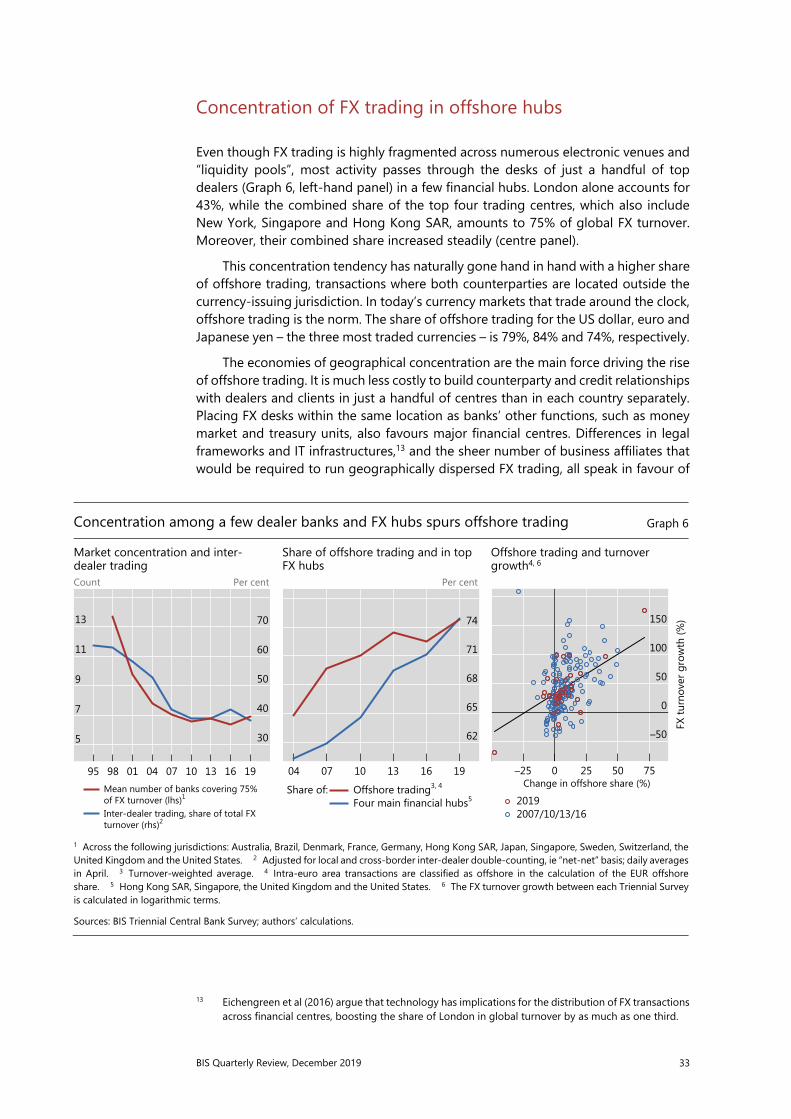
BIS Quarterly Review, December 2019 33
Concentration of FX trading in offshore hubs
Even though FX trading is highly fragmented across numerous electronic venues and “liquidity pools”, most activity passes through the desks of just a handful of top dealers (Graph 6, left-hand panel) in a few financial hubs. London alone accounts for 43%, while the combined share of the top four trading centres, which also include New York, Singapore and Hong Kong SAR, amounts to 75% of global FX turnover. Moreover, their combined share increased steadily (centre panel).
This concentration tendency has naturally gone hand in hand with a higher share of offshore trading, transactions where both counterparties are located outside the currency-issuing jurisdiction. In today’s currency markets that trade around the clock, offshore trading is the norm. The share of offshore trading for the US dollar, euro and Japanese yen – the three most traded currencies – is 79%, 84% and 74%, respectively.
The economies of geographical concentration are the main force driving the rise of offshore trading. It is much less costly to build counterparty and credit relationships with dealers and clients in just a handful of centres than in each country separately. Placing FX desks within the same location as banks’ other functions, such as money market and treasury units, also favours major financial centres. Differences in legal frameworks and IT infrastructures,13 and the sheer number of business affiliates that would be required to run geographically dispersed FX trading, all speak in favour of
13 Eichengreen et al (2016) argue that technology has implications for the distribution of FX transactions
across financial centres, boosting the share of London in global turnover by as much as one third.
Concentration among a few dealer banks and FX hubs spurs offshore trading Graph 6
Market concentration and inter-dealer trading
Share of offshore trading and in top FX hubs
Offshore trading and turnover growth4, 6
Count Per cent Per cent
1 Across the following jurisdictions: Australia, Brazil, Denmark, France, Germany, Hong Kong SAR, Japan, Singapore, Sweden, Switzerland, the United Kingdom and the United States. 2 Adjusted for local and cross-border inter-dealer double-counting, ie “net-net” basis; daily averages in April. 3 Turnover-weighted average. 4 Intra-euro area transactions are classified as offshore in the calculation of the EUR offshoreshare. 5 Hong Kong SAR, Singapore, the United Kingdom and the United States. 6 The FX turnover growth between each Triennial Surveyis calculated in logarithmic terms. Sources: BIS Triennial Central Bank Survey; authors’ calculations.
13
11
9
7
5
70
60
50
40
30
191613100704019895Mean number of banks covering 75%of FX turnover (lhs)1 Inter-dealer trading, share of total FX turnover (rhs)2
74
71
68
65
62
191613100704
Offshore trading3, 4
Four main financial hubs5Share of:
150
100
50
0
–50
7550250–25Change in offshore share (%)
20192007/10/13/16
FX tu
rnov
er g
row
th (%
)

34 BIS Quarterly Review, December 2019
geographical concentration.14 In particular, major dealers tend to consolidate their electronic trading business in one of the major FX hubs. This concentration thus partly compensates for the decentralised OTC structure of FX markets.
Hence, a rise in the share of offshore trading is associated with a rise in that currency’s trading volume, and vice versa (Graph 6, right-hand panel, and in line with regression results reported in Table 1). For example, the decline in the turnover in the Malaysian ringgit between 2016 and 2019 is consistent with authorities effectively prohibiting offshore MYR trading. The relatively slow growth of renminbi trading is also in line with the fall in the share of offshore renminbi (CNH) trading (see Box B).
Conclusion
Global FX volumes recovered from the lows recorded in the previous BIS Triennial Survey. FX trading volumes were buoyed by a pickup in trading with financial clients, such as smaller banks, hedge funds and principal trading firms. Prime brokerage volumes thus saw a rebound across all instruments, which was particularly visible in spot. A strong pickup in trading of FX swaps, especially by smaller banks, was the largest single contributor to overall FX turnover growth, and largely owed to the crucial role of these instruments in banks’ funding liquidity management.
The 2019 Triennial results also point to the increased footprint of non-bank electronic market-makers, a subset of the broader class of principal trading firms. These new players provide FX intermediation services by substituting speed for balance sheet. Their larger FX market presence, now also in direct relationship trading akin to that of bank dealers, has become vital to understanding liquidity conditions and market functioning.
The dominance of financial trading motives and further electronification of FX trading, particularly in the dealer-customer segment, has been conducive to further concentration of trading in a few financial hubs where e-trading is booked. Hence, more geographically concentrated trading, aided by technology, compensates to some extent for the otherwise highly fragmented nature of FX markets.
14 For example, there are three main Equinix data centres and internet exchange sites: London (LD4),
New York (NY4) and Tokyo (TY4). Major electronic brokers and FX dealers co-locate their servers in these locations, and so do the more sophisticated FX clients.
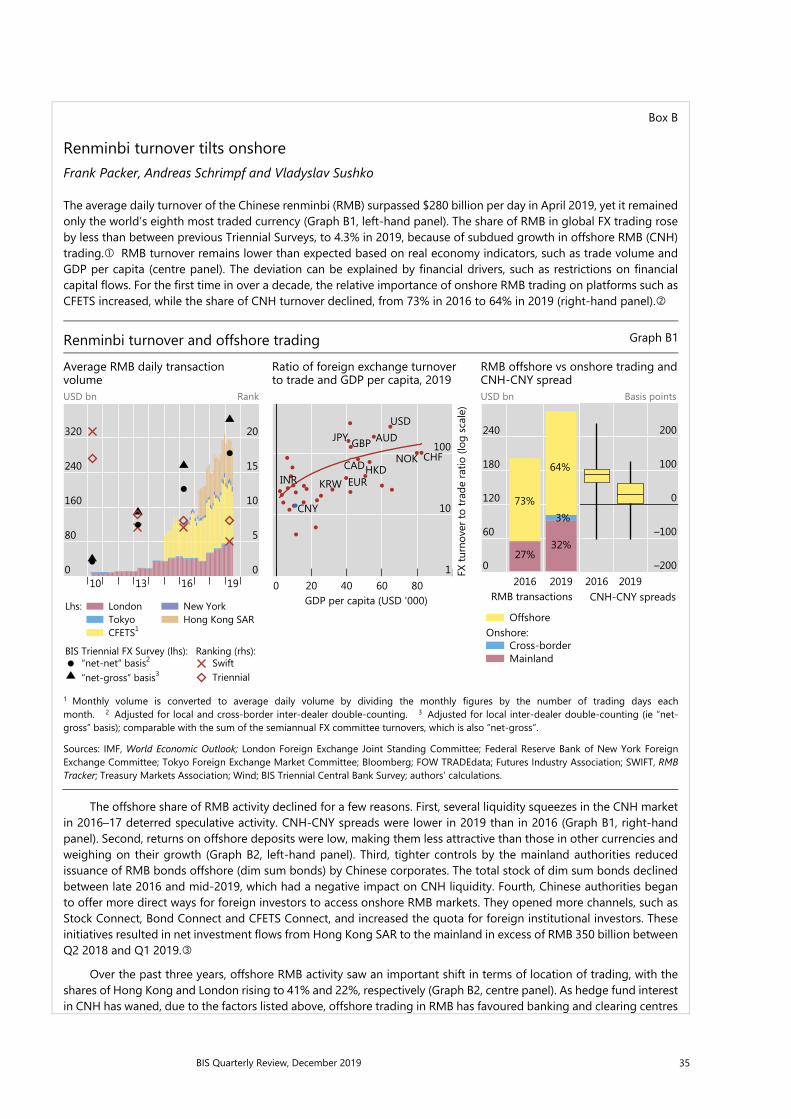
BIS Quarterly Review, December 2019 35
Box B
Renminbi turnover tilts onshore Frank Packer, Andreas Schrimpf and Vladyslav Sushko
The average daily turnover of the Chinese renminbi (RMB) surpassed $280 billion per day in April 2019, yet it remained only the world’s eighth most traded currency (Graph B1, left-hand panel). The share of RMB in global FX trading rose by less than between previous Triennial Surveys, to 4.3% in 2019, because of subdued growth in offshore RMB (CNH) trading. RMB turnover remains lower than expected based on real economy indicators, such as trade volume and GDP per capita (centre panel). The deviation can be explained by financial drivers, such as restrictions on financial capital flows. For the first time in over a decade, the relative importance of onshore RMB trading on platforms such as CFETS increased, while the share of CNH turnover declined, from 73% in 2016 to 64% in 2019 (right-hand panel).
Renminbi turnover and offshore trading Graph B1
Average RMB daily transaction volume
Ratio of foreign exchange turnover to trade and GDP per capita, 2019
RMB offshore vs onshore trading and CNH-CNY spread
USD bn Rank USD bn Basis points
1 Monthly volume is converted to average daily volume by dividing the monthly figures by the number of trading days eachmonth. 2 Adjusted for local and cross-border inter-dealer double-counting. 3 Adjusted for local inter-dealer double-counting (ie “net-gross” basis); comparable with the sum of the semiannual FX committee turnovers, which is also “net-gross”. Sources: IMF, World Economic Outlook; London Foreign Exchange Joint Standing Committee; Federal Reserve Bank of New York ForeignExchange Committee; Tokyo Foreign Exchange Market Committee; Bloomberg; FOW TRADEdata; Futures Industry Association; SWIFT, RMB Tracker; Treasury Markets Association; Wind; BIS Triennial Central Bank Survey; authors’ calculations.
The offshore share of RMB activity declined for a few reasons. First, several liquidity squeezes in the CNH market in 2016–17 deterred speculative activity. CNH-CNY spreads were lower in 2019 than in 2016 (Graph B1, right-hand panel). Second, returns on offshore deposits were low, making them less attractive than those in other currencies and weighing on their growth (Graph B2, left-hand panel). Third, tighter controls by the mainland authorities reduced issuance of RMB bonds offshore (dim sum bonds) by Chinese corporates. The total stock of dim sum bonds declined between late 2016 and mid-2019, which had a negative impact on CNH liquidity. Fourth, Chinese authorities began to offer more direct ways for foreign investors to access onshore RMB markets. They opened more channels, such as Stock Connect, Bond Connect and CFETS Connect, and increased the quota for foreign institutional investors. These initiatives resulted in net investment flows from Hong Kong SAR to the mainland in excess of RMB 350 billion between Q2 2018 and Q1 2019.
Over the past three years, offshore RMB activity saw an important shift in terms of location of trading, with the shares of Hong Kong and London rising to 41% and 22%, respectively (Graph B2, centre panel). As hedge fund interest in CNH has waned, due to the factors listed above, offshore trading in RMB has favoured banking and clearing centres
320
240
160
80
0
20
15
10
5
019161310
LondonTokyoCFETS1
Lhs:
“net-net“ basis2
“net-gross“ basis3
BIS Triennial FX Survey (lhs):
New YorkHong Kong SAR
SwiftTriennial
Ranking (rhs):
USD
EUR
JPY GBP AUD
CHFCADHKD
KRW
NOK
INR
CNY
100
10
1806040200
GDP per capita (USD '000)
FX tu
rnov
er to
trad
e ra
tio (l
og s
cale
)
.27%
32%
240
180
120
60
020192016
3%
64%
73%
RMB transactions
Offshore
Cross-borderMainland
Onshore:
200
100
0
–100
–20020192016
CNH-CNY spreads

36 BIS Quarterly Review, December 2019
with direct onshore links, most notably in Hong Kong. Hence, in April RMB ranked fifth in SWIFT (Graph B1, left-hand panel), which captures bank-to-bank payment flows. London has also continued to increase its status as a leading offshore hub for RMB, having displaced Singapore as the largest trading centre for RMB outside greater China.
In contrast with the decelerating growth in overall RMB turnover, central bank reserves held in RMB rose significantly in recent years, with official institutions accounting for 51% of total turnover by foreign institutional investors by Q3 2018. RMB turnover involving official sector counterparties grew from a daily average of $1.1 billion to $2.0 billion over the last three years. At the same time, the RMB’s share in total FX reserves almost doubled from 1% in 2016 to nearly 2% in 2019, equivalent to about $200 billion (Graph B2, right-hand panel), further evidence of the increased attention of the public sector to investment opportunities in RMB. RMB reserve allocations have benefited from the authorities’ stepwise process of opening up onshore markets, as well as relatively high returns compared with other fixed income instruments and good diversification properties relative to other reserve currencies.
Offshore RMB deposits, trading by location and share in official reserves Graph B2
Offshore deposits Location of trading outside mainland China, 20193
Share of global foreign exchange reserves in renminbi
CNY bn Per cent Per cent
1 Data are available from Q2 2012 (as a part of CGFS enhancements) and the coverage is partial. 2 Australia, Canada, Denmark, Japan, Norway, Sweden, Switzerland, the United Kingdom and the United States. 3 As a total of CNY trading excluding mainland China. Sources: People’s Bank of China; CEIC; BIS locational banking statistics by residence and Triennial Central Bank Survey.
CNH is used to refer to offshore RMB activity, CNY onshore activity. In addition to intervention in the market, the People’s Bank of China also imposed a reserve requirement on the offshore renminbi in 2016. See eg Ehlers et al (2016). Citi Research (2019). This is consistent with the prediction of Cheung et al (2019). Rigaudy (2019).
2,000
1,500
1,000
500
01917151311
HKTWKR
SGEuro area1
MO
Otherdevelopedcountries1, 2
16% (–5)
22% (+2)
41% (+3)
9% (+1)
11% (–1)
Hong Kong SARSingaporeUnited Kingdom
United StatesRest
1.6
1.2
0.8
0.4
0.0
19181716151413

BIS Quarterly Review, December 2019 37
References
Bech, M (2012): “FX volume during the financial crisis and now”, BIS Quarterly Review, March, pp 33–43. Borio, C, R McCauley and P McGuire (2017): “FX swaps and forwards: missing global debt?”, BIS Quarterly Review, September, pp 37–54. Borio, C, R McCauley, P McGuire and V Sushko (2016): “Covered interest parity lost: understanding the cross-currency basis”, BIS Quarterly Review, September, pp 45–64. Cheung, Y W, R McCauley and C Shu (2019): “Geographic spread currency trading: the renminbi and other EM currencies”, BIS Working Papers, no 806. Chitu, L, B Eichengreen and A Mehl (2014): “When did the dollar overtake sterling as the leading international currency? Evidence from the bond markets”, Journal of Development Economics, vol 111, pp 225–45. Du, W, A Tepper and A Verdelhan (2018): “Deviations from covered interest rate parity”, Journal of Finance, vol 73, no 3, pp 915–57. Ehlers, T, F Packer and F Zhu (2016): “The changing landscape of renminbi offshore and onshore markets”, BIS Quarterly Review, December, pp 72–3. Eichengreen, B, R Lafarguette and A Mehl (2016): “Cables, sharks and servers: technology and the geography of the foreign exchange market”, NBER Working Paper, no 21884, January. Federal Reserve Bank of New York (2005): “Foreign exchange prime brokerage, product overview and best practice recommendations”, Annual Report, pp 33–46. Hasbrouck, J and R Levich (2017): “FX market metrics: New findings based on CLS bank settlement data”, NBER Working Paper, no 23206. Hong Kong Monetary Authority (2018): “Linked exchange rate system operations – mechanism and theory”, Research Memorandum, 11/2018, December. Krohn, I and V Sushko (2019): “FX spot and swap market liquidity spillovers”, BIS Working Papers, forthcoming. McCauley, R and M Scatigna (2011): “Foreign exchange trading in emerging currencies: more financial, more offshore”, BIS Quarterly Review, March, pp 67–75. Moore, M, A Schrimpf and V Sushko (2016): “Downsized FX markets: causes and implications”, BIS Quarterly Review, December, pp 35–51. Patel, N and D Xia (2019): “Offshore markets drive FX trading of emerging market currencies”, BIS Quarterly Review, December, pp 53–67. Rigaudy, J-F (2019): “Renminbi reserves are still relatively small”, Central Banking, February. Rime, D, A Schrimpf and O Syrstad (2017): “Segmented money markets and covered interest parity arbitrage”, BIS Working Papers, no 651, July. Schrimpf, A and V Sushko (2019): “FX trade execution: complex and highly fragmented”, BIS Quarterly Review, December, pp 39–51.

38 BIS Quarterly Review, December 2019
Annex table
Global FX market turnover in April 2019, by counterparty and instrument Net-net basis,¹ daily averages in April 2019 Table A Turnover in
2019 2016–19 change
2016–19 change
Contribution to 2016–19
change USD bn In per cent
Global FX market 6,595 1,529 30% 100% By counterparty Reporting dealers 2,523 403 19% 26%
Other financial institutions 3,599 1,034 40% 68% Of which:
Non-reporting banks 1,616 502 45% 33% Institutional investors 777 –21 –3% –1% Hedge funds and principal trading firms 593 204 52% 13%
Official sector financial institutions 89 15 21% 1% Other2 499 317 174% 21%
Non-financial customers 474 92 24% 6% By instrument Spot 1,987 335 20% 22% Outright forwards 999 300 43% 20% FX swaps 3,203 825 35% 54% Currency swaps 108 26 32% 2% Options 298 43 17% 3% 1 Adjusted for local and cross-border double-counting. Turnover and absolute change rounded. Undistributed volumes omitted from thetable. 2 This category can include various other financial counterparties, such as securities firms, financial arms of corporates, retailaggregators or institutions performing the role of so-called prime of prime (see Moore et al (2016)). Sources: BIS Triennial Central Bank Survey; authors’ calculations.
39
FX trade execution: complex and highly fragmented1
The 2019 Triennial Survey shows that trade execution has undergone rapid change, with more diverse participants, new technologies and increasing complexity. Electronification advanced the fastest in dealer-to-customer trading. Dealers and customers navigated a highly fragmented market by leveraging technology to trade across electronic venues. Aspects of FX intermediation tilted more towards non-banks as new market-makers, albeit brokered by top dealers. Bank dealers continued to attract large flows to their own proprietary liquidity pools. Consequently, even though the market grew bigger as a whole, the share of trading activity `visible´ to the broader market declined. JEL classification: C42, C82, F31, G12, G15.
For many years, the BIS Triennial Central Bank Survey2 has chronicled changes in the structure of foreign exchange (FX) markets and the way trades are executed, meaning where and how orders are filled. The latest survey shows that trade execution has undergone rapid change. FX trading is turning more electronic, participants are becoming more diverse, and trading venues are multiplying. These innovations have enhanced the speed of trading, offered participants more choices and facilitated a greater variety of trading strategies.
This special feature first describes how FX markets have become increasingly complex and fragmented. It then analyses recent developments in trade execution in different market segments in general, and the growth of electronic trading in particular. The concluding section discusses the possible implications of these changes for the resilience of FX markets. A box takes a close look at a crucial element of the post-trade ecosystem – how market participants mitigate FX settlement risk.
1 The authors would like to thank Benjamin Anderegg, Sirio Aramonte, Morten Bech, Claudio Borio,
Alain Chaboud, Yin-Wong Cheung, Stijn Claessens, Jenny Hancock, Brian Hardy, Henry Holden, Wenqian Huang, Thomas Maag, Robert McCauley, Dagfinn Rime, Takeshi Shirakami, Hyun Song Shin, and Philip Wooldridge for input. We also greatly appreciate the feedback and insightful discussions with numerous market participants at major FX dealer banks, buy-side institutions, electronic market-makers and trading platforms. We are also grateful to Yifan Ma and Denis Pêtre for compiling the underlying data and Adam Cap for excellent research assistance. The views expressed are those of the authors and do not necessarily reflect those of the Bank for International Settlements.
2 For information about the Triennial Survey, see www.bis.org/statistics/rpfx19.htm.
Andreas [email protected]
Vladyslav [email protected]

40 BIS Quarterly Review, December 2019
The feature complements the analysis of the main drivers of recent growth in global FX turnover in Schrimpf and Sushko (2019) in this issue.
An increasingly complex and fragmented market structure
FX trading has become more complex and fragmented over the years.3 FX markets were long characterised by a two-tier structure, with clearly delineated inter-dealer and dealer-customer segments. This structure has blurred somewhat over the years (Graph 1). Financial institutions outside the bank dealer community have taken on important intermediation functions, and a plethora of electronic trading venues have emerged. These developments have led to ever greater choice in how to execute trades but also to a highly fragmented market structure.
An important catalyst of these developments was prime brokerage, whereby top FX dealers allow clients to trade directly in the bank’s name with its established counterparties. Principal trading firms (PTFs) are some of the heaviest users of prime brokerage services. PTFs employ algorithmic trading strategies and have been active in FX for quite some time. What is new in recent years is that some have built a business model around making markets and thus have deeply penetrated the realm that previously was exclusive to dealers (see Schrimpf and Sushko (2019) in this issue). Prime brokered trading now accounts for a large fraction of volumes on platforms that historically catered to interbank trading, such as electronic brokers.4
The proliferation of alternative ways to conduct trades has been spurred by customers “shopping around” for best execution and by technology providers facing lower costs to set up such platforms. Another trend has been the use of liquidity aggregators that bundle access to different trading venues or liquidity providers (Oomen (2017)). Countering this tendency, FX dealer banks, in turn, have sought to build stronger relationships with their customers. They have invested heavily in improving the technology and functionality of their proprietary trading platform offerings, known as single-bank platforms.
3 King et al (2012) illustrate the gradual build-up of complexity of the market from the 1980s through
the first decade of the 2000s. We add a layer to capture further developments over the past decade. 4 Another set of players, not discussed further in this article, are retail clients (eg individuals, family
offices or smaller hedge funds). Their trading needs are served by retail brokerage platforms or retail aggregators (denoted by RA in Graph 1). Their market access has become one-step removed from wholesale FX markets because of their reliance on so-called “prime-of-prime”, as discussed by Moore et al (2016).
Key takeaways
• Electronification advanced most rapidly in dealer-to-customer trading, while the electronic share of inter-dealer trading decreased.
• A rise in intermediation within dealers’ proprietary liquidity pools contributed to a decline in the share of “visible” FX trading in spot markets.
• Customers and dealers responded to market fragmentation by executing trades across a large number of electronic venues.

41
The resulting fragmentation of the FX market has made it harder to assess market conditions at any given point in time. Market participants wishing to trade FX have more than 75 different FX venues at their disposal (Sinclair (2018)).5 At the same time, greater internalisation of customer flow by banks (explained below) reduced the amount of inter-dealer trading via the main electronic brokers. Thus, while the market as a whole grew bigger, the share of trading activity that is “visible” to the broader market declined. Against this background, the execution methods data collected in the Triennial Survey provide a unique and rare perspective on how the structure of this crucial, yet inherently opaque, market has evolved.
Mapping out trade execution using the Triennial Survey
The taxonomy used in the Triennial Survey to capture data on execution methods is aligned with the main features of the market structure sketched above. At the broadest level, it distinguishes between “voice” and “electronic” execution. Within each, it further differentiates between “direct” (bilateral) and “indirect” (brokered) trading. “Direct” includes relationship-based trading by phone, trades through a chatting system, via a proprietary single-bank platform, or a direct electronic price
5 These venues differ in terms of the pool of participants (eg composition of fast (algorithmic) vs slow
(human) traders, or banks vs non-bank players), microstructural aspects affecting latency, the order queuing or cancellation process of the platform’s matching engine, ”last-look” (ability of liquidity providers to reject the trade even after their price quotes are hit) policies, as well as the suite of different trading protocols.
Stylised structure of the FX market Graph 1
EB = electronic broker; LA = liquidity aggregator; MBP = multi-bank platform; PB = prime broker; PTF = principal trading firm; RA = retailaggregator; SBP = single-bank platform; VB = voice broker. Dashed lines indicate voice execution; solid lines indicate electronic execution. Source: King et al (2012), augmented by adding LA to depict liquidity aggregators and PTFs in their roles as both clients and intermediaries.

42 BIS Quarterly Review, December 2019
stream. “Indirect” refers to the involvement of a third party in the matching process. This can, for instance, be a traditional voice broker, an electronic broking platform or a multi-bank platform.
The 2019 Triennial Survey data on execution methods corroborate the picture of great diversity in trade execution choices. Electronic trading dominates, although voice remains significant in some market segments (Graph 2, left-hand panel and Annex Table A). Electronic trading was roughly equally split between “direct” and “indirect” trading in 2019, whereas “direct” electronic trading had a significantly higher market share three years earlier. Drilling down further into various forms of electronic trading, direct forms of electronic execution were about equally split between single-bank platforms and other direct forms of electronic trading, such as price streams (Graph 2, right-hand panel). When it comes to indirect electronic trading, “anonymous” venues, where counterparty identities are only revealed post-trade, attracted a slightly higher market share than “disclosed” venues, where counterparties know each other’s identity before they decide to trade.
How is the landscape of FX trade execution evolving?
The main trend in FX trade execution has been increased “electronification”– deeper penetration of the market by electronic and automated trading. Electronification comes in a variety of forms, catering to the needs of a diverse set of players (fast and slow traders, banks and non-banks etc). It enables automated and continuous trading, bringing together participants with diverse trading interests so that they can more seamlessly adjust and redistribute financial exposures.
The 2019 Triennial Survey shows that the share of FX trading executed electronically edged up only slightly since the previous survey (Graph 3, left-hand
How were FX trades executed in April 2019? Percentage shares in total turnover Graph 2
Broad voice and electronic execution methods1 Breakdown of electronic execution methods
1 Change in percentage points since the 2016 Triennial Survey indicated in brackets. 2 “Direct” refers to trades not intermediated by a thirdparty. 3 “Indirect” refers to trades intermediated by a third party – either a voice broker or a third-party electronic platform. 4 Single-bank trading systems (eg Barclays BARX, Citi Velocity, Deutsche Bank Autobahn, UBS Neo). 5 Other direct electronic trading systems (eg directelectronic price streams). 6 Multi-bank dealing systems that facilitate trading on a disclosed basis or that allow for liquidity partitioningusing customised tags (eg 360T, EBS Direct, Currenex FXTrades, Fastmatch, FXall OrderBook, Hotspot Link). 7 Electronic trading platforms geared to the non-disclosed inter-dealer market (eg EBS Market, Hotspot FX ECN, Reuters (Refinitiv) Matching). Sources: BIS Triennial Central Bank Survey; authors’ calculations.
13 (–2)
27 (0)29 (+6)
28 (–5)
3 (+1)
Voice direct2
Voice indirect3Electronic direct2
Electronic indirect3Undistributed
16
13
13
1550
40
30
20
10
0
Single-bank platforms4
Other5
Electronic direct:Disclosed venues6
Anonymous venues7
Electronic indirect:
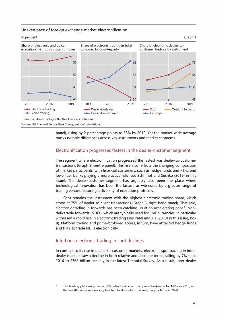
43
panel), rising by 2 percentage points to 58% by 2019. Yet the market-wide average masks notable differences across key instruments and market segments.
Electronification progresses fastest in the dealer-customer segment
The segment where electronification progressed the fastest was dealer-to-customer transactions (Graph 3, centre panel). This rise also reflects the changing composition of market participants, with financial customers, such as hedge funds and PTFs, and lower-tier banks playing a more active role (see Schrimpf and Sushko (2019) in this issue). The dealer-customer segment has arguably also been the place where technological innovation has been the fastest, as witnessed by a greater range of trading venues featuring a diversity of execution protocols.
Spot remains the instrument with the highest electronic trading share, which stood at 75% of dealer-to-client transactions (Graph 3, right-hand panel). That said, electronic trading in forwards has been catching up at an accelerating pace.6 Non-deliverable forwards (NDFs), which are typically used for EME currencies, in particular witnessed a rapid rise in electronic trading (see Patel and Xia (2019) in this issue, Box B). Platform trading and prime-brokered access, in turn, have attracted hedge funds and PTFs to trade NDFs electronically.
Interbank electronic trading in spot declines
In contrast to its rise in dealer-to-customer markets, electronic spot trading in inter-dealer markets saw a decline in both relative and absolute terms, falling by 7% since 2016 to $368 billion per day in the latest Triennial Survey. As a result, inter-dealer
6 The leading platform provider, EBS, introduced electronic prime brokerage for NDFs in 2016, and
Reuters (Refinitiv) announced plans to introduce electronic matching for NDFs in 2020.
Uneven pace of foreign exchange market electronification In per cent Graph 3
Share of electronic and voice execution methods in total turnover
Share of electronic trading in total turnover, by counterparty
Share of electronic dealer-to-customer trading, by instrument1
1 Based on dealer trading with other financial institutions. Sources: BIS Triennial Central Bank Survey; authors’ calculations.
55
50
45
40201920162013
Electronic tradingVoice trading
62
58
54
50201920162013
Dealer-to-dealer Dealer-to-customer1
75
65
55
45201920162013
SpotFX swaps
Outright forwards

44 BIS Quarterly Review, December 2019
trading accounted for less than a third of the total electronic spot market in 2019, 10 percentage points lower than in 2016 (Graph 4, left-hand panel).
This decline in electronic inter-dealer trading was driven principally by internalisation, whereby dealers temporarily warehouse risk arising from client transactions until it is offset against opposing client flow. This practice, in turn, reduces the need to offload any imbalances in inter-dealer markets. Data showed dealers reporting in the United Kingdom and the United States had some of the largest declines in electronic trading on anonymous inter-dealer venues (Graph 4, left-hand panel) and also posted some of the highest internalisation ratios for spot trades (Graph 4, centre panel).
As a consequence, electronic inter-dealer brokerage systems, which have long constituted the main locus of electronic inter-dealer trading, now only account for a small fraction of the entire market. As Evans and Rime (2019) highlight, order book depth on these platforms also declined in tandem. A likely factor has been greater algorithmic trading (Graph 4, right-hand panel), especially by PTFs (on a prime brokered basis), which tends to involve greater activity at the top of the order book. Despite this, these so-called primary venues (eg EBS Market and Reuters (Refinitiv) Matching) are still vital for FX market functioning. Primary venues still serve as an important point of price discovery (Markets Committee (2018)), and when volatility rises, internalisation becomes more challenging and dealers need these venues to manage inventory imbalances (Moore et al (2016)).
More internalisation also means that fewer trades are visible in the broader marketplace, resulting in less information leakage (Butz and Oomen (2019)). It likely
Inter-dealer spot e-trading stagnates due to internalisation Graph 4
Inter-dealer e-trading in spot and turnover on Reuters Matching/EBS1
Internalisation ratios for top trading centres3
Algorithmic vs manual on EBS
Per cent USD bn Per cent Per cent
1 The 2019 data also include turnover on other anonymous venues and hence are not directly comparable with the 2016 figures for this data breakdown. 2 Adjusted for local and cross-border inter-dealer double-counting, ie “net-net” basis; daily averages in April. 3 Volume-weighted averages using total customer spot turnover. 4 For the United States, same share of customer spot turnover in total spot turnoveras in the United Kingdom is assumed to calculate the volume-weighted average. 5 Hong Kong SAR, Japan and Singapore. 6 France, Germany and Switzerland. Sources: EBS; BIS Triennial Central Bank Survey; authors’ calculations.
43%42%
32%
19%
13%12%
38%
45%56%
37
34
31
28
25
120
90
60
30
0201920162013
in e-traded spotInter-dealer share
Lhs:USUKAll other
Turnover (rhs):2
80
60
40
20
0UK & US4 Asian Next three
centres5 centres6
All currenciesG4 currencies currencies
Other G10
100
75
50
25
0
191613100704
AlgorithmicManual
Trading type:

45
led to an increase in “on-us” settlement across the books of the dealers.7 Internalisation may also partly explain why the FX industry remains highly concentrated among a few very large dealers. It may contribute to a market structure in which concentration begets more concentration: given that dealers with large flows from a diverse set of clients find it easier to internalise and can price more competitively, letting them attract ever greater customer flows. Indeed, the falling share of inter-dealer trading has gone hand-in-hand with a handful of banks coming to dominate FX volumes.8 By contrast, banks finding it hard to compete turn to other niches to retain an edge (eg providing execution algorithms to clients).
The ability of dealers to internalise benefits greatly from electronification and the ability to attract customers to trading via single-bank platforms or direct price streams. Subdued FX volatility in recent years was also conducive to internalisation. This is because there have been fewer instances of large imbalances in order flow that are difficult to match internally, thus requiring hedging on inter-dealer venues.
FX swaps still rely heavily on voice intermediation
The 2019 Triennial Survey confirms that, despite the overall trend, electronic trading is not progressing uniformly across all instruments and market segments. Most prominently, inter-dealer trading of FX swaps has remained heavily voice-reliant, while dealer-to-customer trading has moved towards greater use of electronic execution methods.
There are several interrelated reasons for voice retaining a higher share in FX swaps. First, swap trades vary greatly in size, with inter-dealer transactions at times involving particularly large notional amounts. Second, FX swaps are more difficult to price, with internal and balance sheet considerations playing a relatively larger role. The largest dealers use internal models to set their prices (eg relying on their money market desk and taking funding rates in different currencies as inputs) as opposed to sourcing price signals from wholesale venues. This means that inter-dealer FX swap trading still often relies on intermediation via voice brokers. Third, FX swap trading entails management of credit risk because it involves exchanging principal in two different currencies, at the spot rate at contract inception and at the forward rate at contract maturity. This risk needs to be managed and allocated across counterparties which, at least so far, still requires some manual processes.
By contrast, electronic trading continues to make inroads into dealer-to-customer FX swap trading. When quoting bid or ask prices to customers, dealers can rely on inter-dealer mid-prices as input. Such trading with customers is more amenable to electronification, eg by streaming prices on a single-bank platform or responding to a request-for-quote on a multi-dealer-platform.
7 On-us settlement is where both legs of a FX transaction are settled across the books of a single
institution. It is not a payment-versus-payment settlement method (see box). 8 On average, desks belonging to seven reporting banks account for 75% of FX turnover in each
jurisdiction. Schrimpf and Sushko (2019) in this issue also show the inverse relationship between concentration and inter-dealer trading.

46 BIS Quarterly Review, December 2019
Further fragmentation as execution spreads across secondary venues
The 2019 Triennial Survey shows that trading on multi-bank platforms (sometimes referred to as “secondary venues” to contrast them with electronic brokers, which are referred to as “primary venues”) constitutes the fastest growing execution method over the past three years. Some of these secondary venues operate anonymous limit order books, akin to those on primary venues. Others cater to disclosed forms of electronic trading, where identities are known to the counterparties before they decide to engage in a trade. This allows some aspects of relationship trading to be retained, while also matching with a broader pool of potential counterparties.
The trend towards greater reliance on methods where end users can choose from a range of liquidity providers and various ways to implement the trade is reinforced by increased attention to best execution. Sophisticated clients increasingly rely on execution algorithms to spread large orders over time and across multiple electronic venues.9 Hedge funds have been the early adopters of execution algorithms, although fund managers have followed suit (Graph 5, left-hand panel).10 As an indication of clients becoming more cost-conscious, trading on multi-bank platforms, or via liquidity aggregators bundling various venues and providers, has surpassed single-bank platform volumes and other direct forms of electronic trading (Graph 5,
9 The cost-efficient execution of large volumes is the primary driver of execution algorithm use. With
automated execution, it is the customers who bear market risk instead of dealer banks. 10 Financial clients, such as money managers, are also under considerable pressure to demonstrate best
execution, with an additional push from regulatory reforms such as MiFID II. Although MiFID II is a European regulation, its global impact is highlighted in the JP Morgan Electronic Trading Trends for
Sophisticated customers spread their electronic trading across venues In per cent Graph 5
Algorithm adoption by global financials1
Electronic trading, dealer-customer segment2
Multi-dealer platform market shares
1 Based on responses from 710 top-tier financial FX users. 2 Based on dealer trading with other financial institutions. 3 Trading executed via single-dealer platforms or other direct electronic execution methods, such as API. 4 Electronic trading intermediated by a third partysuch as via an electronic broking system or electronic communication network. Sources: Euromoney Foreign Exchange Survey 2019; Greenwich Associates 2018 Global Foreign Exchange Study; BIS Triennial Central BankSurvey; authors’ calculations.
25
20
15
10
5
0
fundsmanagersHedgeFundBanks
2013 2016 2018
60
55
50
45
40
35201920162013
Electronic direct share3
Electronic indirect share4
2.7
1.2
1.9
2.9
2.3
9.5
28.3
32.7
7.36.2
5
RefinitivFX ConnectBloombergCurrenex360TEBS
Integral - FX Inside
TechnologiessmartTrade
FXSpotStreamFastMatchOthers
47
centre panel).11 For example, according to the 2019 Euromoney survey, buy-side customers trade using over a dozen different platform providers (Graph 5, right-hand panel).12 It is also common for top-tier liquidity providers (including non-bank market-makers) to cater to this demand by quoting simultaneously on a wide range of venues (Markets Committee (2018)).
Conclusion
FX trading has evolved rapidly over recent years. It has seen further electronification and increasing variety in trading venues and protocols. In spot, FX intermediation has tilted towards non-bank electronic market-makers, who substitute speed for balance sheet. Activity has also gravitated more to dealers’ proprietary liquidity pools and away from primary inter-dealer venues. Clients can use algorithms to enhance execution and navigate a fragmented market, albeit in exchange for taking on more market risk themselves. All these developments have led to more choice for tech-savvy clients, but also to some important risk-shifting and greater market fragmentation.
Yet there are signs that fragmentation may be reaching its peak. Some customers are reportedly questioning the cost of connecting to so many venues. Dealers, too, have been re-assessing whether it is beneficial to quote prices on a large number of third-party systems. For example, a top-tier bank recently announced plans to slash the number of systems it uses, from 45 to 15. Similarly, some PTFs focused on market-making have reportedly also cut down on the number of electronic communication networks where they post prices.
Furthermore, the current market configuration has emerged largely during a prolonged period of low volatility, and its resilience might be tested if the volatility regime were to change. For example, during periods of stress, FX dealers might ration liquidity and favour clients with whom they have a strong relationship, such as those using their single-bank platform. Thus, customers who spread execution across venues could face a sharp evaporation of liquidity. The question of whose risk-bearing capacity to rely on under such circumstances could become a pertinent one. In the event of stress, the resilience of FX markets could be further challenged by the declining use of payment-versus-payment systems to reduce FX settlement risk (see box).
2018 survey: while 73% of respondents in EMEA believe it will have an impact, 47% of respondents in the Americas and 45% in Asia-Pacific also hold the same view.
11 Academic research indicates that clients face less price discrimination when trading FX derivatives through multilateral trading platforms (Hau et al (2019)).
12 Some of the technology providers shown offer more than one platform for customer trading.

48 BIS Quarterly Review, December 2019
FX settlement risk remains significant Morten Bech and Henry Holden
The settlement of FX trades can lead to significant risk exposures when one counterparty to a trade sends a currency payment to the other and needs to wait before receiving the currency it is buying. Over the past two decades, market participants have made significant progress in reducing FX settlement risk. Nevertheless, due in part to higher trading activity, the 2019 Triennial Survey indicates that close to $9 trillion of payments remain at risk on any given day.
The bankruptcy of Bankhaus Herstatt in 1974 demonstrated how FX settlement risk can undermine financial stability. Herstatt was a medium-sized German bank active in FX markets. At 15:30 CET on 26 June 1974, the German authorities closed the bank down. While Herstatt had already received Deutsche marks from its counterparties, it had not yet made the corresponding US dollar payments in New York. Herstatt’s failure to pay led banks more generally to stop outgoing payments until they were sure their countervalues had been received. The international payment system then froze, and the erosion of trust caused lending rates to spike and credit to be curtailed.
FX settlement risk: increasing and global Graph A.1
FX settlement methods1 Proportion of settlements with PvP protection2
CLS-ineligible currency pairs
Per cent Per cent USD bn Per cent
1 “PvP settlement” includes settlement through systems such as CLS and Hong Kong CHATS. 2 The median value is represented by ahorizontal line, with 50% of the values falling in the range shown in the box. The highest and lowest values are represented by the upper andlower end points of the vertical lines. Sources: Committee on Payment and Settlement Systems, “Progress in reducing foreign exchange settlement risk“, CPMI Papers, no 83, May 2008; D Kos and R Levich, “Settlement risk in the global FX market: how much remains?“, SSRN, October 2016; BIS Triennial Central Bank Survey; authors’ calculations.
In 1996, G10 central banks endorsed a strategy to reduce FX settlement risk. The strategy involved actions to be taken by banks to control their exposures, actions to be taken by industry groups to provide services and actions to be taken by central banks to induce progress. In response, in 2002 market participants set up Continuous Linked Settlement (CLS), a specialist institution that settles FX transactions on a payment-versus-payment (PvP) basis. PvP eliminates FX settlement risk by ensuring that a payment in a currency occurs if and only if the payment in the other currency takes place. The establishment of CLS and other actions led to a big reduction in FX settlement risk. Even at the height of the Great Financial Crisis, FX markets remained resilient. However, FX settlement risk appears to have increased since 2013 in both relative and absolute terms (Graph A.1, left-hand panel).
To help assess progress in reducing FX settlement risk, the Triennial Survey was expanded in 2019 to collect data on FX settlement. Different FX instruments give rise to different numbers of payments. For example, spot and outright forwards result in two payment obligations, whereas swaps result in four payments of principal (two at inception and
75
50
25
02019201320061997
settlementNon-PvP
PvP settlementnettingPre-settlement
75
50
25
0
currenciescurrencies without CLSwith CLS
CountriesCountriesEMEsAEs
Interquartile range Median
1,200
800
400
0
20
15
10
52019201620132010
Lhs:
Rhs:(average total daily turnover)CLS-ineligible currency pairs
(share of total turnover)CLS-ineligible currency pairs

49
two at repayment). Some FX transactions, such as non-deliverable forwards, are settled with a single payment and are therefore not subject to FX settlement risk. FX trades can also be bilaterally netted, which eliminates a need for settlement.
After taking account of the number of payments for each instrument, in April 2019 daily global FX trading of $6.6 trillion translated into gross payment obligations worth $18.7 trillion (Table A.1). Bilateral netting reduced the payment obligations to $15.2 trillion. About $6.3 trillion was settled on a PvP basis using CLS or a similar settlement system. This left an estimated $8.9 trillion worth of FX payments at risk on any given day. The proportion of trades with PvP protection appears to have fallen from 50% in 2013 to 40% in 2019, although available data are not fully comparable across time (Graph A.1, left-hand panel).
One reason for the relative decline in PvP protection is the growth of trading in currencies not eligible for CLS settlement. In absolute terms, 90% of FX settlement risk is in the top 10 jurisdictions. However, these advanced economies settle a higher proportion of their FX with PvP protection than emerging market economies (EMEs) do, many of which have currencies that are not included in CLS (Graph A.1, centre panel). Nonetheless, CLS-eligible currency pairs still make up about 80% of total global trading activity (Graph A.1, right-hand panel). To reduce global risk, it may therefore be necessary to both encourage FX market participants to use PvP where available and widen that availability to include EME currencies. The task of reducing global risk is now firmly on the agenda of bank supervisors.
G Galati, “Settlement risk in foreign exchange markets and CLS Bank”, BIS Quarterly Review, December 2002, pp 55–65. Committee on Payment and Settlement Systems, “Settlement risk in foreign exchange transactions“, CPMI Papers, no 17, March 1996. Basel Committee on Banking Supervision, “Basel Committee discusses policy and supervisory initiatives and approves implementation reports”, press release, October 2019.
Trading activity and payments Table A.1
Description Trades/payments Trading activity USD billions A. Spot 1,987 B. Deliverable forwards 741 C. FX and currency swaps 3,311 D. NDFs and options1 556 E. Total (= A + B + C + D) 6,595 Settlement F. Gross payment obligations (= 2 × (A + B) + 4 × C) 18,701 G. Bilateral netting2 (3,516) H. Net payment obligations (F – G) 15,185 I. Of which: settled with PvP3 6,311 J. Of which: settled without PvP protection4 8,874 1 NDFs and some options are settled with a single payment and are therefore not subject to FX settlement risk. 2 Bilateral netting reduces the amount of payment obligations to be settled; it is calculated by applying the proportion of netting shown in the Triennial Survey. 3 Calculated using the CLS settlement data for April 2019 and the “Other PvP” proportion in the Triennial Survey. 4 “Without PVP protection” is the residual. Sources: CLS; BIS Triennial Central Bank Survey; authors’ calculations.
50 BIS Quarterly Review, December 2019
References
Butz, M and R Oomen (2019): “Internalisation by electronic FX spot dealers”, Quantitative Finance, vol 19, no 1, pp 35–56. Euromoney (2019): Foreign Exchange Survey 2019: Electronic trading. Evans, M and D Rime (2019): “Microstructure of foreign exchange markets”, SSRN, February. Greenwich Associates (2019): FX execution: competing in a world of algos. Hau, H, P Hoffmann, S Langfield and Y Timmer (2019): “Discriminatory pricing of over-the-counter derivatives”, IMF Working Papers, no 19/100. King M, C Osler and D Rime (2012): “Foreign exchange market structure, players and evolution”, in Handbook of Exchange Rates, edited by I Marsh, J James, and L Sarno, Hong Wiley & Sons. Moore, M, A Schrimpf and V Sushko (2016): “Downsized FX markets: causes and implications”, BIS Quarterly Review, December, pp 35–51. Markets Committee (2018): “Monitoring of fast-paced electronic markets”, Markets Committee Papers, no 10, September. Oomen, R (2017): “Execution in an aggregator”, Quantitative Finance, vol 17, no 3, pp 383–404. Patel, N and D Xia (2019): “Offshore markets drive trading of emerging market currencies”, BIS Quarterly Review, December, pp 53–67. Schrimpf, A and V Sushko (2019): “Sizing up global foreign exchange markets”, BIS Quarterly Review, December, pp 21–38. Sinclair, J (2018): “Why does fragmentation continue to increase? Increasing entropy in currency markets”, MarketFactory Whitepaper, February.

Execution method by instrument and counterparty in 2019, percentage shares Net-net basis,¹ daily averages in April 2019, in per cent Annex Table A Voice Electronic Electronic direct Electronic indirect Counterparty sector
Instrument Voice total Direct2 Indirect3 Electronic
total Electronic direct total
Single-bank platforms4 Other direct5 Electronic
indirect total Anonymous
venues6 Disclosed venues7
All counterparties
Spot 28 25 3 69 32 17 15 37 26 11 FX swaps 46 24 21 52 26 14 12 26 12 14 Outright forwards 38 31 7 57 29 13 16 28 13 15 Currency swaps 77 63 14 19 13 3 9 7 1 6 Options 65 50 15 31 21 19 2 10 3 7
Reporting dealers
Spot 33 28 5 62 34 20 14 28 15 14 FX swaps 50 26 25 48 23 12 10 25 12 13 Outright forwards 48 37 11 46 28 15 13 18 9 9 Currency swaps 80 66 15 18 9 2 8 8 1 7 Options 60 44 16 33 21 19 2 12 5 7
Other financial institutions
Spot 24 23 1 73 29 14 15 44 34 11 FX swaps 42 23 19 55 28 14 14 27 12 15 Outright forwards 31 26 6 64 29 12 17 35 17 18 Currency swaps 76 62 14 22 16 4 12 6 1 5 Options 69 54 16 29 19 18 1 10 3 7
Non-financial customers
Spot 35 31 3 64 45 21 24 19 9 10 FX swaps 39 27 11 60 36 21 15 24 4 20 Outright forwards 52 45 7 45 30 13 17 15 3 12 Currency swaps 51 47 4 18 15 8 7 3 0 3 Options 63 54 9 33 28 24 5 5 1 4
Percentage shares of total FX volumes for each counterparty segment and instrument; totals do not total 100 due to incomplete reporting. 1 Adjusted for local and cross-border inter-dealer double-counting. 2 “Direct” refers to trades not intermediated by a third party. 3 “Indirect” refers to deals intermediated by a third party, ie either a voice or an electronic broker. 4 Single-bank trading systems (eg Barclays BARX, Citi Velocity, Deutsche Bank Autobahn, UBS Neo). 5 Other direct electronic trading systems as well as direct electronic price streams. 6 Electronic trading platforms geared towards the non-disclosed inter-dealer market (eg, EBS Market, Hotspot FX ECN, Refinitiv Matching). 7 Multi-bank dealing systems that facilitate trading on a disclosed basis or that allow for liquidity partitioning using customised tags (eg 360T, EBS Direct, Currenex FXTrades, Fastmatch, Refinitiv FXall Order Book, Hotspot Link). Sources: BIS Triennial Central Bank Survey; authors' calculations.


BIS Quarterly Review, December 2019 53
Offshore markets drive trading of emerging market currencies1
FX markets for the currencies of emerging market economies grew more rapidly than those for major currencies between 2016 and 2019, rising from 19% to almost 25% of global turnover. At the same time, these currencies attracted a wider range of participants and saw a rapid increase in offshore trading activity. Offshore markets tended to drive onshore markets during times of global market stress.
JEL classification: F31, G12, G23.
In foreign exchange (FX) markets, the trading of emerging market economy (EME) currencies outgrew that of major currencies between 2016 and 2019. While global turnover rose by 33%, the turnover of EME currencies rose by almost 60% over this period, to $1.6 trillion. This article highlights recent trends in the trading of EME currencies and discusses the main drivers of their recent growth.
One notable trend in EME currency trading was an increase in the share of trading generated by hedge funds, proprietary trading firms (PTFs) and other financial customers. A second trend was a surge in offshore trading. An important driver here was the growing appetite of global investors for EME assets. In addition, the electronification of FX trading enabled smaller players to participate in a market traditionally dominated by inter-dealer trading among large banks. Finally, activity continued to be influenced by restrictions on currency convertibility.
The remainder of this article is organised as follows. The next section describes the growth in FX markets for EME currencies between 2016 and 2019, drawing on data from the BIS Triennial Central Bank Survey.2 We then detail changes in the composition of market participants, instruments and trading venues and analyse their drivers. The last section summarises the key policy implications.
1 The authors would like to thank Claudio Borio, Michael Chui, Stijn Claessens, Mathias Drehmann,
Bryan Hardy, Robert McCauley, Benoît Mojon, Denis Pêtre, Andreas Schrimpf, Hyun Song Shin, Vladyslav Sushko, Christian Upper and Philip Wooldridge for helpful comments and Samuel Carrasco for excellent research assistance and comments. The views expressed here are those of the authors and do not necessarily reflect those of the Bank for International Settlements.
2 For information about the Triennial Survey, see www.bis.org/statistics/rpfx19.htm.
Nikhil [email protected]
Dora [email protected]

54 BIS Quarterly Review, December 2019
Growth of FX trading in EME currencies
For many years, FX trading in EME currencies has outgrown that of advanced economy (AE) currencies. The average daily turnover of EME currencies rose by almost 60% between April 2016 and April 2019, to almost $1.6 trillion (Graph 1, left-hand panel). This boosted the share of EME currencies in global turnover to 23%, up from 19% in 2016 and 15% in 2013.
The increase in FX turnover was particularly pronounced in many Asian currencies (Graph 2). The Chinese renminbi was the most traded EME currency, at $289 billion per day in April 2019, but its 48% growth between 2016 and 2019 was moderate when compared with that of many other currencies (see Packer et al (2019) in this issue).
Trading in the Indian rupee, Indonesian rupiah and Philippine peso more than doubled, despite continued restrictions on their convertibility. In contrast, many of the more freely convertible EME currencies, such as the Mexican peso, Singapore dollar and South African rand, experienced below average growth. The Hong Kong
Key takeaways
• Markets for EME currencies grew faster than those for major currencies between 2016 and 2019. • Global demand for emerging market assets and the electronification of trading drove recent growth. • During times of FX market stress, offshore markets for EME currencies tend to drive onshore prices.
Turnover in EMEs FX markets continued to rise Graph 1
Total FX turnover in EME currencies1, 2
FX derivatives vs spot in EME currencies in 20191, 3
Change in FX turnover vs international trade and external assets between 2016 and 20194
Per cent USD bn
1 OTC data are adjusted for local and cross-border inter-dealer double-counting. EME currencies = ARS, BRL, CLP, CNY, COP, CZK, HKD, HUF,IDR, INR, KRW, MXN, MYR, PEN, PHP, PLN, RUB, SAR, SGD, THB, TRY and ZAR. Turnover at constant exchange rate in April 2019. 2 FX data include OTC (spot, outright forwards, FX swaps, currency swaps and options) and exchange-traded transactions (futures and options). 3 FX derivatives = Total OTC turnover minus spot transactions for each currency plus exchange-traded transactions. Slope is statistically significantat 1% level. 4 ARS excluded from the sample. 5 Sum of merchandise exports and imports over 12 months to April of each year. 6 External assets (from the international investment position) as of Q1; for Malaysia, Q4 2018. Slope is statistically significant at the 5% level. Sources: IMF, Balance of Payments and Direction of Trade Statistics; national data; BIS Triennial Central Bank Survey; authors’ calculations.
25
20
15
10
5
1,400
1,050
700
350
0
19161310070401
global turnoverShare in
Lhs:Over-the-counter
derivativesExchange-traded
Rhs:
CNY
KRW
MXN
HKD
INRSGDBRL
RUB
TRY
160
120
80
40
0
150100500
y = 2.21xwhere R2 = 0.80
45°
FX spot (USD bn)
FX d
eriv
ativ
es (U
SD b
n)
y = 29.1 +1.76x where R2 = 0.215
HK
MY
PH180
120
60
0
–60
6040200
Total trade5 IIP assets6Percentage change in:
Chan
ge in
FX
tota
l tur
nove
r (%
)1, 2

BIS Quarterly Review, December 2019 55
dollar stood out with one of the largest increases in turnover, due probably to temporary factors in April 2019 related to local funding conditions.
A notable exception to the rapid increase in EME currencies’ turnover was the Malaysian ringgit, which experienced a 48% decline in turnover between 2016 and 2019. New administrative restrictions contributed to the sharp decline in ringgit turnover. The Malaysian authorities banned offshore trading of non-deliverable forwards (NDFs) by domestic entities.3 As a result, offshore trading in the ringgit collapsed between 2016 to 2019. While measures were also introduced to promote onshore trading, the rise in onshore trading could not outweigh the decline in offshore trading.
For EME currencies, as for AE currencies, the turnover of FX derivatives greatly exceeded spot transactions. Derivatives trading in EME currencies approached $1.1 trillion per day in April 2019, whereas spot trading was less than $0.5 trillion. The volume of derivatives trading was, on average, double that of spot trading for both EME and AE currencies (Graph 1, centre panel).4 Notable exceptions included the Mexican peso and Russian rouble, where derivatives trading in April 2019 was low relative to spot trading, and the Hong Kong dollar, where derivatives trading was relatively high. For most EME currencies, the FX derivatives markets were larger and more developed than those for interest rate derivatives (see Box A).
In line with global patterns, trading on over-the-counter (OTC) markets greatly exceeded that on exchanges. For EME currencies, OTC FX derivatives accounted for 95% of the total turnover, slightly below their 98% global share.5 In April 2019, exchange-traded derivatives accounted for a substantial share of activity in only two currencies: the Brazilian real (36%) and the Indian rupee (13%).
3 NDFs are forward contracts that do not involve an actual exchange of currencies. Instead, they entail
a settlement of the difference between the actual and a pre-agreed exchange rate in a single US dollar payment at maturity.
4 The ratio understates spot trading because, in the Triennial Survey, the spot leg of FX swaps is not reported. This bias is more sizeable for AE currencies, given their larger share of FX swaps trading.
5 The dominant share of OTC markets is partly explained by the greater flexibility that OTC deals offer to meet special demands, such as for specific maturities and trading currency pairs not involving the US dollar (Wooldridge and Xia (2019)). While the US dollar remained dominant, as the currency on one side of 99% of all trades on exchanges in April 2019, its share in OTC markets was lower, at 90%.
Turnover in most EME currencies grew, particularly in emerging Asia Total FX turnover by currency, daily average turnover in April1 Graph 2
USD bn
1 OTC transactions are adjusted for local and cross-border inter-dealer double-counting. Data include OTC (spot, outright forwards, FX swaps,currency swaps and options) and exchange-traded transactions (futures and options). Sources: BIS derivatives statistics and Triennial Central Bank Survey; authors’ calculations.
225
150
75
0
30
20
10
0ARSPENMYRSARCOPPHPCLPCZKHUFIDRTHBPLNTRYZARRUBBRLMXNSGDINRKRWHKDCNY
Lhs Rhs
2019 2016, at constant exchange rate

56 BIS Quarterly Review, December 2019
Box A
FX instruments dominate derivatives markets in EMEs The relative size of FX and interest rate derivatives markets differs markedly between EMEs and AEs. The turnover of interest rate derivatives in EMEs rose significantly between April 2016 and April 2019, increasing from $173 billion to $273 billion (Graph A1, left-hand panel). Nevertheless, in April 2019, the turnover of FX derivatives denominated in EME currencies was still more than four times greater than that of interest rate derivatives. This was in stark contrast to AE currencies, where trading in the two asset classes was on a more equal footing. In the right-hand panel of Graph A1, the red line suggests that the ratio of interest rate to FX derivatives turnover is much smaller than one for EME currencies on average, indicating that FX instruments predominate in EME derivatives markets. In comparison, the blue line, for AEs, revealed more activity in interest rate derivatives than in FX derivatives.
FX outweighs interest rate instruments in EME derivatives trading Graph A1
Interest rate derivatives turnover in EME currencies1 FX and IR derivatives turnover in EME currencies in 20192
Per cent USD bn
1 EME currencies = ARS, BRL, CLP, CNY, COP, CZK, HKD, HUF, IDR, INR, KRW, MXN, MYR, PEN, PHP, PLN, RUB, SAR, SGD, THB, TRY and ZAR; AE currencies = AUD, CAD, CHF, EUR, GBP, JPY, NOK, NZD, SEK and USD. Interest rate derivatives include OTC (forward rate agreements,options, overnight indexed swaps, other interest rate swaps and other instruments). OTC derivatives are adjusted for local and cross-border inter-dealer double-counting. Turnover at constant exchange rate in April 2019. 2 FX derivatives = OTC and XTD excluding spot transactions.IR derivatives = OTC and XTD transactions. Blue line corresponds to AEs; red line corresponds to EMEs. Sources: BIS derivatives statistics and Triennial Central Bank Survey; authors’ calculations.
The notional amounts outstanding painted a similar picture. For EME currencies, FX and interest rate derivatives markets were similar in size, whereas for AE currencies interest rate derivatives volumes exceeded those of FX derivatives by a large margin (see Aramonte and Huang (2019) in this issue).
The smaller scale of interest rate derivatives activity in EMEs, as compared with AEs, reflected several factors. Less-developed bond markets and benchmark rates in EMEs meant more limited demand for interest rate derivatives. In addition, tighter control of capital markets in EMEs further curbed demand, by restricting the investor base. The EMEs that stood out in terms of interest rate derivatives activity were Mexico and South Africa, which have better developed bond markets than most other EMEs, as well as freely convertible currencies.
Changes in the turnover of interest rate derivatives varied considerably across currencies (Annex Table A1, second and third columns). Most Asian currencies witnessed significant increases. In particular, renminbi interest rate derivatives increased more than threefold, overtaking the Mexican peso as the most actively traded EME instrument in this category. On the other side of the spectrum, interest rate derivatives trading declined in several Latin American currencies (Argentine peso, Chilean peso, Colombian peso and Peruvian sol). See Ehlers and Hardy (2019) in this issue for an overview of recent trends in global interest rate derivatives markets.
4
3
2
1
0
240
180
120
60
0
19161310070401
turnoverShare in global
Lhs:Over-the-counterExchange-traded derivatives
Rhs:
BRL
CLP
CNY
CZK
HKDINR
KRW
MXN
PLNRUB
SGD
TRY
ZAR
48
36
24
12
0
200150100500
y = 2.003xwhere R2 = 0.965
y = 0.224xwhere R2 = 0.506
FX derivatives (USD bn)
IR d
eriv
ativ
es (U
SD b
n)

BIS Quarterly Review, December 2019 57
Evolving market structure
Two notable trends have characterised the FX market for EME currencies in recent years; first, the increased presence of non-bank financial institutions; second, the rapid growth in forwards, in particular NDFs, and the related increased role of offshore transactions.
Rising prominence of non-bank financial institutions
In general, the growth of FX trading is linked more strongly to financial motivations than to trade in goods and services. In the right-hand panel of Graph 1, the orange line shows a positive relationship across EMEs between the growth in gross external financial assets and FX turnover. By contrast, the black line shows that the relationship between trade in goods and services and FX turnover was much weaker.6 These results accord with the dominant role of financial factors in driving activity in FX markets, as documented elsewhere (eg Schrimpf and Sushko (2019a) in this issue).
Consistent with the dominant role of financial factors, the recent growth in FX turnover for EME currencies was led by trading with non-bank financial institutions (NBFIs). This contrasts with AE currencies, where smaller (non-dealer) banks played
6 Interestingly, growth in gross external financial liabilities plays a less significant role, probably
reflecting that EME liabilities consist mainly of equity and foreign direct investments, which generate less turnover owing to both their longer term and lower hedging requirements.
Growth of EME currencies trading was driven by non-bank financial institutions1
In per cent Graph 3
OFIs are increasingly important counterparties for EME currencies2
Market ecosystem for EME currencies becomes more like that in AEs3
EME currencies = ARS, BRL, CLP, CNY, COP, CZK, HKD, HUF, IDR, INR, KRW, MXN, MYR, PEN, PHP, PLN, RUB, SAR, SGD, THB, TRY and ZAR; AE currencies = AUD, CAD, CHF, EUR, GBP, JPY, NOK, NZD, SEK and USD. Counterparty: RD = reporting dealers; Banks = non-reporting banks; NBFI = non-bank financial institutions; NFC = non-financial customers; HF & PTFs = hedge funds and proprietary trading firms; Others = others and undistributed. 1 FX OTC daily average turnover in April adjusted for local and cross-border inter-dealer double-counting. 2 Growth rate in FX turnover in April 2019 with respect to April 2016 at constant exchange rate for EME and AE currencies. Spot transactions included. 3 FX OTC turnover in 2019 by counterparty as percentage of turnover by all counterparties. Spot transactions included. Sources: BIS Triennial Central Bank Survey; authors’ calculations.
160
120
80
40
0
AEEMEAEEME
388
RDNBFINFCBanks
Counterparty:
100
75
50
25
0
AEEMEAEEME
InstitutionalsHF and PTFSOfficial sectorOthers
NBFIs:

58 BIS Quarterly Review, December 2019
the leading role (Graph 3, left-hand panel). Among NBFIs, the rise of “other” financial institutions (those not categorised as institutional investors, hedge funds, property trading firms or the official sector) was especially pronounced. This category includes retail aggregators.
These developments brought the composition of market participants more into line with that of AE currencies (Graph 3, right-hand panel). However some differences remained. For example, despite growing at a faster rate over the past three years, the share of institutional investors continued to be smaller in EME currencies than in AE currencies.
The rising share of NBFIs reflects increased non-bank and foreign demand for EME assets as financial intermediation shifts from banks to capital markets in EMEs. For example, the participation of foreign investors in local currency bond markets in EMEs has increased (BIS (2019)). Assets under management by dedicated EME equity and bond funds have doubled over the past decade (Graph 4, left-hand panel). In contrast, bank demand for EME assets has moderated. The share of banks in the Malaysian government bond market, for example, has fallen markedly over the last three years (Graph 4, centre panel).
Hedge funds and PTFs, which are active in algorithmic trading, also saw swifter increases, as compared with their activity in AE currencies. This rise is attributable in large part to the continuing electronification of global FX markets (see Holden et al (2019) in this issue). As shown by the blue bars in the right-hand panel of Graph 4, electronic trading of EME currencies grew at a faster pace in derivatives than in the spot market.
Rising demand for non-bank EME assets and growing electronification Graph 4
Total net assets in EMEs Non-resident holdings of Malaysian government bonds
Electronic trading has become more important for EME currencies1, 2
USD bn Per cent Ratio Per cent
1 Trading of USD/Latin American currency pairs (ARS, BRL, CLP and MXN) in North America. Data for April and October. 2 Total FX OTC turnover that involves all electronic execution methods in derivative instruments (FX swaps and outright forwards) over the total FX turnover that involves spot transactions. Sources: Federal Reserve Bank of New York; EPFR; national data; BIS Triennial Central Bank Survey; authors’ calculations.
2,000
1,500
1,000
500
0
1916131007
Bond Equity
100
75
50
25
0
181716
Asset managersPensions and insurersCentral banks
BanksOthers
2.0
1.5
1.0
0.5
0.0
48
36
24
12
0
1916131007
over spot (lhs)in derivativesElectronification
(rhs)execution in totalShare of electronic
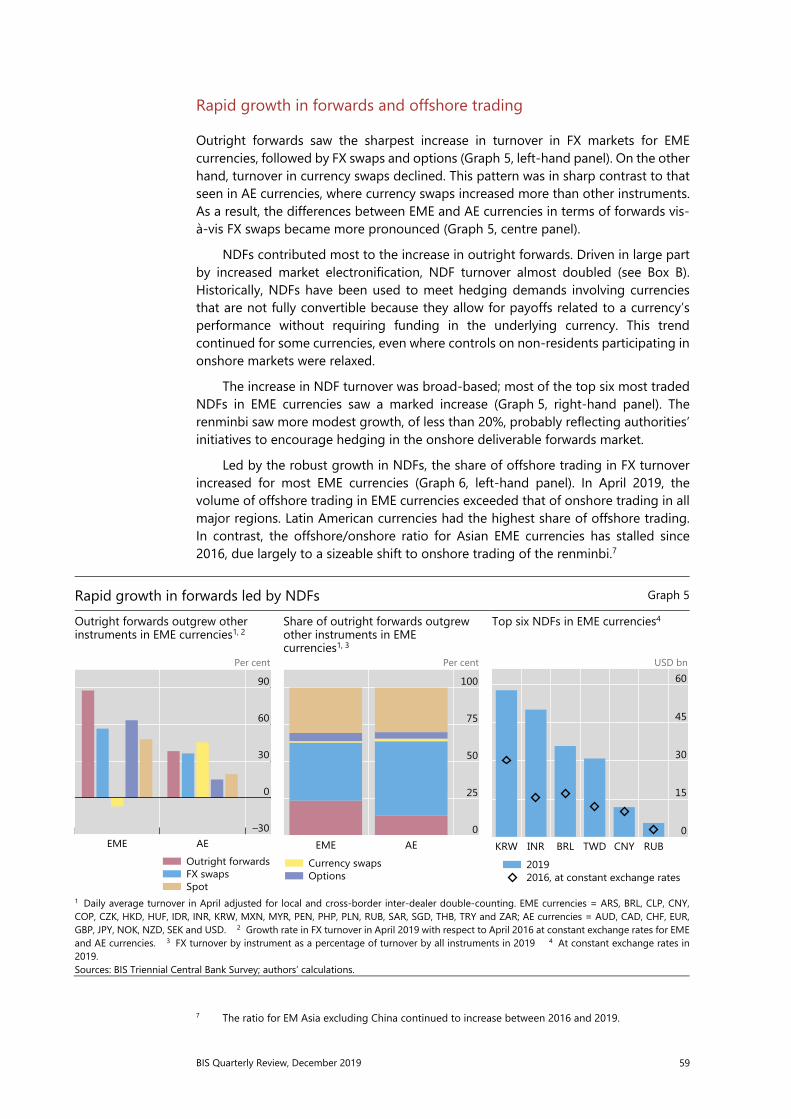
BIS Quarterly Review, December 2019 59
Rapid growth in forwards and offshore trading
Outright forwards saw the sharpest increase in turnover in FX markets for EME currencies, followed by FX swaps and options (Graph 5, left-hand panel). On the other hand, turnover in currency swaps declined. This pattern was in sharp contrast to that seen in AE currencies, where currency swaps increased more than other instruments. As a result, the differences between EME and AE currencies in terms of forwards vis-à-vis FX swaps became more pronounced (Graph 5, centre panel).
NDFs contributed most to the increase in outright forwards. Driven in large part by increased market electronification, NDF turnover almost doubled (see Box B). Historically, NDFs have been used to meet hedging demands involving currencies that are not fully convertible because they allow for payoffs related to a currency’s performance without requiring funding in the underlying currency. This trend continued for some currencies, even where controls on non-residents participating in onshore markets were relaxed.
The increase in NDF turnover was broad-based; most of the top six most traded NDFs in EME currencies saw a marked increase (Graph 5, right-hand panel). The renminbi saw more modest growth, of less than 20%, probably reflecting authorities’ initiatives to encourage hedging in the onshore deliverable forwards market.
Led by the robust growth in NDFs, the share of offshore trading in FX turnover increased for most EME currencies (Graph 6, left-hand panel). In April 2019, the volume of offshore trading in EME currencies exceeded that of onshore trading in all major regions. Latin American currencies had the highest share of offshore trading. In contrast, the offshore/onshore ratio for Asian EME currencies has stalled since 2016, due largely to a sizeable shift to onshore trading of the renminbi.7
7 The ratio for EM Asia excluding China continued to increase between 2016 and 2019.
Rapid growth in forwards led by NDFs Graph 5
Outright forwards outgrew other instruments in EME currencies1, 2
Share of outright forwards outgrew other instruments in EME currencies1, 3
Top six NDFs in EME currencies4
Per cent Per cent USD bn
1 Daily average turnover in April adjusted for local and cross-border inter-dealer double-counting. EME currencies = ARS, BRL, CLP, CNY,COP, CZK, HKD, HUF, IDR, INR, KRW, MXN, MYR, PEN, PHP, PLN, RUB, SAR, SGD, THB, TRY and ZAR; AE currencies = AUD, CAD, CHF, EUR, GBP, JPY, NOK, NZD, SEK and USD. 2 Growth rate in FX turnover in April 2019 with respect to April 2016 at constant exchange rates for EME and AE currencies. 3 FX turnover by instrument as a percentage of turnover by all instruments in 2019 4 At constant exchange rates in 2019. Sources: BIS Triennial Central Bank Survey; authors’ calculations.
90
60
30
0
–30AEEME
Outright forwardsFX swapsSpot
100
75
50
25
0AEEME
Currency swapsOptions
60
45
30
15
0RUBCNYTWDBRLINRKRW
20192016, at constant exchange rates

60 BIS Quarterly Review, December 2019
Strictly offshore trades (where both counterparties are located offshore) dominate the market for FX turnover in EME currencies (Graph 6, centre panel). By the location of a trade, defined as the location of the sales desk of the reporting dealer, a trade can be classified as either “strictly domestic” (between two parties located onshore), “onshore-offshore” (between one party located onshore and the other offshore) or “strictly offshore” (both parties located offshore).
The rapid expansion of strictly offshore trading was broad-based (Annex Table A2).8 Except for the Hong Kong dollar and the Malaysian ringgit, all other EME currencies were traded mainly between two parties located outside the domestic jurisdiction as of April 2019.
The vast majority of offshore FX transactions in EME currencies took place in a handful of locations. London played the most notable role, followed by New York, Singapore and Hong Kong SAR.
The prominence of offshore trading is not specific to EME currencies. It reflects the network effects that have led to a highly concentrated market structure within a handful of global financial centres. For EME currencies, capital account and currency convertibility restrictions represent an additional factor behind the higher share of offshore trading. In particular, jurisdictions with heavier capital account restrictions tend to have a higher share of offshore trading of derivatives (Graph 6, right-hand panel). In other words, capital controls appeared to boost the offshore trading of derivatives – NDFs in particular – at the expense of onshore trading.
8 The Triennial Survey might overstate “strictly offshore” trading. Dealers report whether a trade is
local, with a resident counterparty, or cross-border, with a non-resident. Therefore, trades between dealers located offshore and customers located onshore are included with offshore trades.
Share of offshore transactions increased in most regions Graph 6
OTC offshore-to-onshore turnover1, 2 FX turnover in EME currencies by counterparty location2, 3
Chinn-Ito index and offshore-to-onshore ratio in EME currencies4
Ratio USD bn
1 Emerging Asia = CNY, HKD, IDR, INR, KRW, MYR, PHP, SGD and THB; Latin America = ARS, BRL, CLP, COP, MXN and PEN; Other EMEs =CZK, HUF, PLN, RUB, SAR, TRY and ZAR. 2 Onshore transactions are defined as the turnover in the corresponding currency in the issuingjurisdiction (on a net-gross basis). Offshore transactions are defined as the difference between the total turnover of a currency on a net-net basis and the onshore transactions in the issuing jurisdiction. Includes total OTC derivatives and spot transactions. Excludes exchange-traded transactions. 3 EME currencies = ARS, BRL, CLP, CNY, COP, CZK, HKD, HUF, IDR, INR, KRW, MXN, MYR, PEN, PHP, PLN, RUB, SAR, SGD, THB,TRY and ZAR. 4 Offshore-to-onshore turnover in OTC FX derivatives in 2019. ARS, CZK, HUF, MYR, and PLN excluded from the sample. Thep-value of the slope coefficient equals 0.11 in a one-sided t-student distribution with 15 degrees of freedom. Sources: BIS Triennial Central Bank Survey; authors’ calculations.
3
2
1
0191613100704
AsiaEmerging Latin America
Other EMEs
1,200
800
400
0191613100704
On/offshore On/onshoreOff/offshore
9
6
3
01.00.80.60.40.2
y = 4.88 –2.39xwhere R2 = 0.0984
Chinn-Ito index (2017)
Off/
onsh
ore
ratio
FX
deriv
ativ
es (2
019)

BIS Quarterly Review, December 2019 61
Box B
NDF markets thrive on the back of electronification Andreas Schrimpf and Vladyslav Sushko
Trading of NDFs has almost doubled over the past three years, contributing significantly to the substantial increase in the trading of forwards recorded in the 2019 Triennial Survey. NDFs are contracts that, unlike their deliverable counterparts, settle in the same currency (typically the US dollar) at maturity, based on the movement of the underlying exchange rate. NDFs are particularly popular for trading non-convertible currencies. The key currencies behind the NDF surge include the Korean won, Brazilian real, Indian rupee and New Taiwan dollar (Graph B1, left-hand panel).
Evolution of NDF trading by currency and location, and central clearing Graph B1
NDF trading by currency1 Share of cleared instruments NDF trading by location2 Per cent USD bn Per cent Per cent
1 Adjusted for local and cross-border inter-dealer double-counting, ie “net-net” basis; daily averages in April. 2 Change since the 2016 Triennial Survey in brackets, in percentage points. 3 For the United Kingdom, the share of electronic trading (electronic broking and trading systems) is calculated based on FXJSC April 2019 survey data. Sources: London Foreign Exchange Joint Standing Committee Survey (FXJSC); US Commodity Futures Trading Commission Swap Reports; BIS Triennial Central Bank Survey; authors’ calculations.
Hedge funds and PTFs can trade NDFs to arbitrage or take directional bets. In the process, they serve as natural counterparties to market participants who need to hedge currency exposures. NDFs exemplify two main trends in the structure of global FX markets, as highlighted in the main text: (i) electronification of trading with other financial institutions, and (ii) concentration of trading activity in the largest FX centres.
The trend towards electronification in NDF markets rides on the inclusion of these instruments among those traded on the main electronic broking platforms: EBS emerged as the electronic venue for NDF trading, while Reuters (Refinitiv) Matching plans to launch NDF trading in 2020. Electronification has also benefited from central clearing, which enables multilateral netting and reduces the need to post margins. As highlighted in McCauley and Shu (2016), the NDF market microstructure has started evolving rapidly on the back of global legal and regulatory reforms for derivatives markets. Since 2015, NDFs have started the transition from a decentralised, bilateral microstructure to one characterised by centralised trading, disclosure and clearing. The gradual phase-in of uncleared margin rules, requiring firms to post initial margins for certain uncleared derivatives, has incentivised greater central clearing of NDFs. To date, NDFs represent the only type of FX derivative with any meaningful share of centrally cleared transactions (Graph B1, centre panel).
These forces have naturally led to a further concentration of trading in the main FX hubs, with the share of NDF trading in the United Kingdom more than doubling from 20% in 2016 to 46% in 2019 (Graph B1, right-hand panel). Given the popularity of NDF trading in Asian currencies, London’s overlap with the trading hours of Hong Kong SAR and Singapore puts the city in an advantageous position.
13% 14% 14%14% 12%
19%15% 23%
22%
7% 9%
12%
51%43%
32%
25
20
15
10
5
0
250
200
150
100
50
0
201920162013
Rhs:Share in total forward turnover BRLINRKRW
Lhs:TWDOther
5
4
3
2
1
0
25
20
15
10
5
0
Q3 2019Q2 2019Q1 2019Q4 2018
Cross-currencySwaps & forwardsExoticsOptions
Lhs: NDFsRhs:
16 (–7)
10 (–5)
16 (–10)
12 (–4)
46 (+26)
e/tradedof which:
United Kingdom3
United States Singapore Hong Kong SAR Other locations

62 BIS Quarterly Review, December 2019
Policy implications
The rapid expansion of offshore trading in EME currencies presents both opportunities and challenges. On the one hand, offshore trading can increase liquidity and cut transaction costs. Electronification can encourage trading by a wider range of market participants, while overlapping time zones allow round-the-clock trading. Increased FX liquidity can in turn boost foreign investment and trade in goods and services.
On the other hand, offshore trading can influence the price discovery process for exchange rates, in markets that are more difficult than onshore centres for central banks to monitor. Estimates for the four largest NDF currencies suggest that, while a bidirectional relationship exists between the onshore and offshore markets during normal times, offshore venues tend to drive movements in the onshore markets during times of global market stress (Box C). This raises challenges for central banks, which have historically limited their market monitoring and intervention policies to the onshore market.
Many central banks have responded to the challenges posed by offshore markets by expanding their monitoring activities. They can expand their coverage of fast-paced electronic markets by tapping larger volumes of data from more diverse sources. They can also enhance the scope and coverage of their market intelligence-gathering efforts (Markets Committee (2016, 2018)). The Korean authorities, for instance, have encouraged domestic entities to play a greater role in offshore markets, with the aim of increasing their monitoring capabilities for offshore markets via these entities. The move has also served to integrate the on- and offshore markets, reducing price discrepancies between the two.
Other central banks, such as those in Indonesia, Malaysia and Turkey, have taken steps to deepen their nascent onshore derivatives markets, often acting as the primary providers of liquidity. Initiatives such as extending onshore trading hours and providing more flexibility for foreign investors to hedge their positions in the domestic markets have also been considered (Reserve Bank of India (2019)).
Furthermore, while spot interventions still remain the dominant intervention tool, some central banks have reacted to the increasing weight of offshore derivatives in the FX market by increasing the use of derivatives in their FX intervention frameworks, including in offshore markets (BIS (2019)).

BIS Quarterly Review, December 2019 63
Box C
How onshore and offshore markets interact: an empirical investigation Understanding the information flow between onshore and offshore markets is of prime importance, particularly for policymakers. It sheds light on the price formation process and reveals the venue of price discovery, which is critical for informing a central bank’s FX intervention strategy and market monitoring efforts.
Policymakers often see spillovers from hard-to-monitor offshore markets as an area of concern (Central Bank of Malaysia (2018)). Indeed, the empirical analysis below shows that, while a bidirectional relationship exists between the onshore and offshore markets during normal times, it turns unidirectional during times of market stress, when offshore markets tend to drive onshore price developments.
In the absence of permanent frictions between the onshore and offshore markets, prices across venues are cointegrated, as confirmed by our empirical estimates. Short-run fluctuations and lead-lag relationships can then be studied using a vector error correction model for onshore spot and forward rates and offshore non-deliverable forward (NDF) rates. This represents the information flow between the onshore and offshore markets, and shows how it varies over time. The model consists of two sets of equations, the first of which captures the long-run relationship between spot and NDF rates. The second set examines how deviations from the long-term relationship affect the short-term dynamics of these rates, an “error correction” mechanism in the spirit of Engel and Granger (1987). This provides information about the direction of the linkage between onshore and offshore markets. The analysis focuses on five currencies with large NDF markets, namely the Brazilian real, Chinese renminbi, Indian rupee, Korean won and New Taiwan dollar.
The long-run equations are as follows: log 𝑠𝑝𝑜𝑡 = 𝛽 + 𝛽 log 𝑁𝐷𝐹 + 𝑒 log 𝑁𝐷𝐹 = 𝛽 + 𝛽 log 𝑠𝑝𝑜𝑡 + 𝑒 β1spot and β1NDF quantify the strength of the long-run relationship between the two exchange rate measures, with a value close to 1 indicating a complete pass-through and the absence of permanent frictions between the two markets.
The short-run equations are as follows: Δ log 𝑠𝑝𝑜𝑡 = 𝛼 + 𝛼 𝑒 + 𝛼 , (Δ log(𝑠𝑝𝑜𝑡 ),… + 𝛼 , (Δ log(𝑁𝐷𝐹) ),… + 𝜖 Δ log(𝑁𝐷𝐹) = 𝛼 + 𝛼 (𝑒 ) + 𝛼 , (Δ log(𝑠𝑝𝑜𝑡) ),… + 𝛼 , (Δ log(𝑁𝐷𝐹) ),… + 𝜖
αspot and αndf are the coefficients of interest. They reveal the rate of adjustment when the system departs from equilibrium. We use them as a measure of the direction of influence. For example, when αspot is negative and statistically significant, it indicates that NDF rates will affect the dynamics of spot rates in the next period.
The analysis reveals, first, that most currencies show a bidirectional relationship: spot prices affect subsequent NDF rates and vice versa. For the Chinese renminbi, Indian rupee and Korean won, this bidirectional relationship holds when the model is estimated over the full sample from January 2005 to October 2019 (Table C1, first row). The New Taiwan dollar stands out as the only currency with unidirectional spillovers from the NDF rates to spot rates. This could reflect the fact that offshore branches of local banks are allowed to participate in the NDF market, which brings additional information to the NDF rates. Unlike the other currencies in the sample, the Brazilian real shows no significant evidence of spillovers from one market to the other. This may reflect the important role that exchange trading plays for the Brazilian real, with price discovery taking place largely in the futures market rather than in the offshore NDF or spot market.
Second, during times of global market stress, it is more likely that the offshore NDF markets will drive onshore prices (Table C1, second to fourth rows). For example, during the Great Financial Crisis (GFC) and the “taper tantrum”, the Indian rupee saw spillovers from the NDF rates to the spot rates but not vice versa. Similar dynamics were also observed for the renminbi and New Taiwan dollar during the GFC, and for the Korean won during the taper tantrum and recent trade tensions. The pattern also manifests itself between the offshore NDF rates and the onshore forward rates (fifth to seventh rows).
The unidirectional influence from offshore to onshore markets during global market stress for Asian currencies likely reflects a number of factors. For one, the onshore and offshore markets span different time zones. As a result, news related to Europe and the United States that arrives during prime trading hours in London and New York is too

64 BIS Quarterly Review, December 2019
late for Asian trading hours. Thus, this news affects NDF rates first, before subsequently affecting the onshore prices the following morning. However, this is probably not the only reason, as the case of the Indian rupee shows. Here Reserve Bank of India (2019) finds the unidirectional flow to hold during market stress episodes, even though the NDF and spot prices are recorded at exactly the same time (the closing time of the onshore market). Other factors, such as different degrees of risk aversion and changes in the wealth of offshore investors during global market stress episodes, could contribute to the unidirectional influence.
Spillovers between onshore rates (spot/forward) and offshore rates (NDF) Table C1
BRL CNY1 INR KRW TWD Spot and NDF Full sample (January 2005–October 2019) × ⇔ ⇔ ⇔ ⇐
GFC (September 2008–July 2009) ⇔ ⇐ ⇐ ⟹ ⇐
Taper tantrum (May 2013–August 2013) ⇔ ⟹ ⇐ ⇐ ×
Trade tensions (May 2018–December 2018) × × × ⇐ ×
Forward and NDF GFC (September 2008–July 2009) ⟹ ⇐ ⇐ ⇐ ⇐
Taper tantrum (May 2013–August 2013) × ⟹ ⇐ ⇐ ×
Trade tensions (May 2018–December 2018) ⇐ × × ⇐ ×
⇔ indicates two-way causality between spot or forward and NDF; ⇐ indicates NDF causes spot or forward; × indicates no relationship. 1 One-month forward data start in 2007. Sources: Bloomberg; authors’ calculations.
In a few cases, spot rates have led the NDF rates during global stress episodes. One example is the Korean won during the GFC. This likely reflects the central bank’s interventions in the onshore markets, which then become the primary venue of price discovery.
The finding that offshore centres tend to lead price discovery during times of stress presents central banks with both opportunities and challenges. The challenge lies in the fact that interventions are primarily restricted to the onshore spot markets, whereas the venues for price discovery during times of stress tend to be the offshore derivatives markets (Cavalino and Patel (2019)). However, the results also indicate that proactive interventions at such times could nevertheless help to counter trends originating in the offshore markets. The approach is similar to the one used in Reserve Bank of India (2019). See also Behera (2011). These results are consistent with prior studies, including McCauley et al (2014). See Annex A in Tsuyuguchi and Wooldridge (2008). For details of price discovery in Brazilian FX markets, see Garcia and Santos (2014). See Garcia and Santos (2014) for how central bank interventions relate to the price discovery process. See Ryoo et al (2013) for the role of the Bank of Korea’s interventions during the GFC.
BIS Quarterly Review, December 2019 65
References
Aramonte, S and W Huang (2019): “OTC derivatives: euro exposures rise and central clearing advances”, BIS Quarterly Review, December, pp 83–93. Bank for International Settlements (2019): Annual Economic Report, Chapter II, “Monetary policy frameworks in EMEs: inflation targeting, the exchange rate and financial stability”. Behera, H (2011): “Onshore and offshore market for Indian rupee: recent evidence on volatility and shock spillover”, in Macroeconomics and Finance in Emerging Market Economies, vol 4, no 1. Cavalino, P and N Patel (2019): “FX intervention: goals, strategies and tactics”, in BIS Papers, no 104, October, pp 25–44. Central Bank of Malaysia (2018): Annual Report, “Monetary and financial conditions in 2018”. Ehlers, T and B Hardy (2019): “The evolution of OTC interest rate derivatives markets”, BIS Quarterly Review, December, pp 69–82. Engle, R and C Granger (1987): “Co-integration and error correction: representation, estimation, and testing”, Econometrica, March, pp 251–76. Garcia, M and F Santos (2014): “Price discovery in Brazilian FX markets”, Textos para discussão, no 622, Department of Economics PUC-Rio (Brazil), May. Markets Committee (2016): “Market intelligence gathering at central banks”, Markets Committee Papers, no 8, December. ——— (2018): “Monitoring of fast-paced electronic markets”, Markets Committee Papers, no 10, September. McCauley, R and C Shu (2016): “Non-deliverable forwards: impact of currency internationalisation and derivatives reform”, BIS Quarterly Review, December, pp 81–93. McCauley, R, C Shu and G Ma (2014): ”Non-deliverable forwards: 2013 and beyond”, BIS Quarterly Review, March, pp 75–88. Packer, F, A Schrimpf and V Sushko (2019): “Renminbi turnover tilts onshore”, BIS Quarterly Review, December, pp 35–6. Reserve Bank of India (2019): Report of the task force on offshore rupee markets, July. Ryoo, S, T Kwon and H Lee (2013): “Foreign exchange market developments and intervention in Korea”, BIS Papers, no 73, October, pp 205–13. Schrimpf, A and V Sushko (2019a): “Sizing up global foreign exchange markets”, BIS Quarterly Review, December, pp 21–38. ——— (2019b): “FX trade execution: complex and highly fragmented”, BIS Quarterly Review, December, pp 39–51. Tsuyuguchi, Y and P Wooldridge (2008): “The evolution of trading activity in Asian foreign exchange markets”, BIS Working Papers, no 252, May. Wooldridge, P and D Xia (2019): “Derivatives trading in OTC markets soars”, BIS Quarterly Review, September, pp 32–3.

66 BIS Quarterly Review, December 2019
Annex tables
Growth in FX was broader-based than for interest rate derivatives1 Table A1
Turnover FX spot and derivatives Interest rate derivatives
2019 level (USD bn)
2019 level (USD bn)
% change from 2016
CNY 289 40 167.4 HKD 233 18 241.5 KRW 135 40 56.5 INR 126 17 179.3 SGD 119 15 23.9 MXN 115 23 –8.6 BRL 102 52 11.4 RUB 74 1 838.7 ZAR 72 26 55.2 TRY 72 1 1,135.3 PLN 41 8 50.6 THB 32 6 183.5 IDR 27 0 –23.2 HUF 27 8 –0.6 CZK 26 12 815.2 CLP 19 1 –64.4 PHP 19 0 61.2 COP 12 1 –25.1 SAR 12 1 41.6 MYR 9 2 –35.1 PEN 5 0 –84.0 ARS 4 0 –80.6 1 Considers FX and IR OTC including spot and exchange traded transactions. Changes are computed at current exchange rates. Sources: BIS Triennial Central Bank Survey; authors’ calculations.

BIS Quarterly Review, December 2019 67
FX turnover in most EME currencies is dominated by offshore trading1 Table A2
Strictly onshore (on-/onshore)2 Strictly offshore (off-/offshore)3 On-/offshore4 2019 level (USD bn)
% change from 2016
2019 level (USD bn)
% change from 2016
2019 level (USD bn)
% change from 2016
BRL 7 –40.7 57 55.4 7 195.9 CNY 92 68.4 184 25.3 9 1279.6 HKD 43 161.4 87 176.3 102 158.9 INR 31 14.9 79 178.8 4 35.2 KRW 34 5.5 84 96.9 14 54.0 MXN 7 37.5 94 20.8 12 –10.5 RUB 20 –26.7 40 84.4 12 38.0 SGD 22 9.3 62 21.2 35 74.8 TRY 5 87.5 59 –3.4 8 –19.4 1 Total OTC turnover, including spot and excluding exchange-traded derivatives. Onshore transactions = turnover in the correspondingcurrency in the issuing jurisdiction (on a net-gross basis). Offshore transactions = the difference between the total turnover of a currency ona net-net basis and the onshore transactions in the issuing jurisdiction. 2 Onshore-onshore = transactions between two counterpartieslocated onshore. 3 Offshore-offshore = transactions between two counterparties located offshore; data about the specific location of customers is not reported in the Triennial Survey, and therefore offshore-offshore may include transactions between offshore dealers andonshore customers. 4 Onshore-offshore = transactions between dealers located onshore and customers offshore. Sources: BIS Triennial Central Bank Survey; authors’ calculations.

BIS Quarterly Review, December 2019 69
The evolution of OTC interest rate derivatives markets1
The trading of interest rate derivatives in over-the-counter (OTC) markets more than doubled between 2016 and 2019, significantly outpacing the growth of trading on exchanges. This rapid expansion was driven by three factors. First, non-market facing trades, such as back-to-back deals and compression trades, increased and were more comprehensively reported in the BIS Triennial Survey. Second, technological developments reduced transaction costs in OTC markets and spurred trading, including more trading by investment funds. And third, changing expectations about US short-term interest rates fuelled hedging and speculative activity. In general, structural developments like clearing, compression and automation remade OTC markets so that they more closely resembled exchanges and led to a relative shift in trading from exchanges to OTC markets. Further market changes due to benchmark rate reforms may be on the horizon. JEL classification: E43, G15, G18, G21, G23.
In recent years, the trading of interest rate derivatives (IRDs) in over-the-counter (OTC) markets has surged. Between April 2010 and April 2016, average daily OTC turnover trended steadily upwards from $2.1 trillion to $2.7 trillion, and then in April 2019 it jumped sharply to $6.5 trillion – an increase of 143% compared with 2016. Trading on exchanges also rose, but not as much (53% between 2016 and 2019). Consequently, whereas OTC trading accounted for only 21% of IRD trading in 2010, it accounted for 46% in 2019.
The increase in OTC trading was driven by a combination of factors. First, the amount and coverage of non-market facing trades expanded, specifically back-to-back and compression trades. Second, the proliferation of electronic trading platforms reduced transaction costs, which in turn incentivised greater trading, especially by investment funds and other asset managers. Third, greater uncertainty around US short-term interest rates fuelled hedging and speculative activity.
These developments were enabled by important structural changes in OTC markets. Regulatory changes incentivised an increase in the use of central clearing,
1 The views expressed in this article are those of the authors and do not necessarily reflect those of the
Bank for International Settlements. We thank Yifan Ma for excellent research assistance, Giulio Cornelli for help with the Lipper data, and LCH Ltd and ClarusFT for providing data. We thank Sirio Aramonte, Claudio Borio, Christian Cabanilla, Stijn Claessens, Wenqian Huang, Patrick McGuire, Denis Pêtre, Vladyslav Sushko, Christian Upper and Philip Wooldridge for helpful comments. We benefited from discussion with numerous market participants and individuals at central banks.
Torsten [email protected]
Bryan [email protected]

70 BIS Quarterly Review, December 2019
electronic trading platforms and portfolio compression services. OTC markets thus acquired many of the same benefits as exchanges, leading to a relative shift in trading from exchanges to OTC markets.
In this feature, we use data from the 2019 BIS Triennial Central Bank Survey of Foreign Exchange and OTC Derivatives Markets to explore the evolution of OTC IRD markets.2 The first section describes the key findings of the 2019 survey. The second discusses the main factors contributing to the increase in IRD turnover. The third section explores how structural developments have affected the relative importance of OTC and exchange trading of IRDs. The final section looks forward to potential future structural changes. A box discusses the shift to central clearing in IRD markets.
A broad-based rise in turnover
Average daily turnover in OTC interest rate derivatives markets more than doubled between the BIS Triennial Surveys in April 2016 and April 2019 (Graph 1, left-hand panel). The 143% increase to $6.5 trillion per day was the highest growth rate since the inception of the surveys in 1995.3 In contrast, between 2007 and 2016, growth between surveys averaged just 17%. Turnover for exchange-traded interest rate derivatives also exhibited high growth between 2016 and 2019, but at 53% was outpaced by OTC turnover. This continued the trend shift in turnover from exchanges to OTC markets that started around 2010.
The surge in OTC turnover was broad-based across instruments and currencies (Graph 1, centre and right-hand panels).4 Interest rate swaps as a whole, which include overnight index swaps (OIS) and basis swaps, remained the most traded instruments, accounting for 64% of the total global turnover (compared with 69% in 2016). Turnover of dollar- and euro-denominated contracts grew by 141% and 148%, respectively, maintaining their global share of OTC turnover (50% and 24%, respectively).
2 The Triennial Survey provides comprehensive information on the size and structure of OTC derivatives
markets. The survey captures, among other things, the aggregate turnover of OTC interest rate derivatives from nearly 1,300 dealers in 53 different jurisdictions. In complement with BIS exchange-traded derivatives (ETD) statistics, they capture activity for interest rate derivatives globally.
3 Compared with monthly data from other sources, April 2019 does not appear to be an exceptional month in terms of OTC turnover. Also, exchange rate movements played a minor role in determining this growth rate. After adjusting for them, the increase was actually a little larger at 147%. Turnover with central counterparties also rose at a very high rate over the same period (115%; see Box A).
4 See also Patel and Xia (2019) in this issue.
Key takeaways
• The daily turnover of OTC interest rate derivatives more than doubled between 2016 and 2019 to $6.5 trillion, taking OTC markets’ share to almost half of total trading.
• Asset managers increased their trading of interest rate derivatives. • Structural changes including clearing, compression and automation made OTC markets more closely
resemble exchanges.

BIS Quarterly Review, December 2019 71
The large increase in dollar and euro IRD turnover was driven by trading in the United States and especially the United Kingdom (Graph 2). In April 2019, sales desks in the UK accounted for over half of all OTC IRD turnover and 86% of euro turnover, up from 39% and 73%, respectively, in 2016 (centre panel). The UK also strengthened its role as the key offshore trading location for emerging market currency contracts (right-hand panel). The United States remained the dominant location for US dollar turnover, expanding from $1.1 trillion to $2 trillion in turnover, though its share of the global amount fell from 80% to 61% between surveys. Dealers in the UK took a substantially larger share in 2019 (left-hand panel).
What drove the increase in turnover?
The increase in turnover was driven by a combination of factors. One factor was more turnover and more comprehensive reporting of non-market facing trades (sometimes referred to as administrative trades), such as back-to-back trades and portfolio compression trades. Yet market-facing trades also increased substantially, boosted by cyclical developments as well as structural shifts in OTC derivatives markets.
More comprehensive reporting and the rise in related party trades
Dealers in several trading jurisdictions noted an increase in related party trades in the 2019 Triennial Survey, in particular back-to-back trades. Related party trades are those between a reporting dealer’s own offices and subsidiaries, or between the dealer and its parent or other affiliated entities. Back-to-back deals are linked deals where the liabilities, obligations and rights of the second deal are exactly the same as those of the original one. They are normally conducted between affiliates of the same consolidated group to facilitate either internal risk management or internal bookkeeping. Back-to-back trades should only be reported to the Triennial Survey if
Turnover and composition in interest rate derivatives markets Notional amounts, daily averages in April1 Graph 1
OTC and exchange-traded markets OTC markets, by instrument OTC markets, by currency Per cent USD trn USD trn USD trn USD bn
1 Adjusted for local and cross-border inter-dealer double-counting, ie “net-net” basis. 2 OIS are included in total swap turnover. Dataavailable only from 2019. 3 Forward rate agreements. 4 CAD, CHF, DKK, NOK, NZD and SEK. 5 AED, ARS, BGN, BHD, BRL, CLP, CNY, COP, CZK, HKD, HUF, IDR, ILS, INR, KRW, MXN, MYR, PEN, PHP, PLN, RON, RUB, SAR, SGD, THB, TRY, TWD and ZAR. Sources: BIS derivatives statistics and Triennial Central Bank Survey.
45
35
25
15
5
12
9
6
3
019161310070401
Share of over-the-counterLhs:Exchange-tradedOver-the-counter
Rhs:
6.0
4.5
3.0
1.5
0.019161310070401
Swaps (total)OIS2
FRAs3
and otherOptions
3.2
2.4
1.6
0.8
0.0
600
450
300
150
0
USD EU
R
GBP
AUD
JPY
Oth
er
EMEs
5 A
Es4
Lhs Rhs
2016Increase from 2016 to 2019

72 BIS Quarterly Review, December 2019
they transfer risk away from the reporting dealer. Feedback from central banks participating in the survey suggests that many reporting dealers that did not fully include these trades in the 2016 survey were able to report them in 2019 (in line with the survey guidelines).5
Related party trades, reported as an “of which” item (without a breakdown by counterparty sector, instrument or currency), jumped significantly, from 15% of total turnover in the 2016 survey to 24% in the 2019 one (Graph 3, left-hand panel). These trades grew by nearly 300% between surveys (centre panel). This boosted positions between reporting dealers (which grew by 124% since the last survey), but also positions between dealers and “other financial institutions” (which grew by 156%).
The pickup in related party trades accounted for about 30% of the OTC increase, or 43 percentage points out of the 143% of total turnover growth. Excluding related party trades, average daily turnover was up 117% since the 2016 survey. This still substantial growth rate is broadly in line with trends evident in other data sources, such as turnover growth at central counterparties (CCPs) (Graph 3, right-hand panel).
In addition to the increased reporting of back-to-back trades, the volume of such trades appears to have gone up. Conversations with dealers and reporting central banks suggest that banks engaged in relatively fewer trades in the inter-dealer market and kept more of their trades within their consolidated group.6 This internalisation would lead to a generic increase in back-to-back trades and contribute to the large amount of related party trades in the 2019 survey.
5 Many dealers began reporting these trades for the first time in 2019. The increased reporting may be
due in part to greater use of electronic trading platforms. The move from voice to electronic booking improved the recording of the details of each trade and made it easier to flag and report back-to-back trades in line with the survey guidelines. Greater emphasis in the reporting guidelines themselves on how such trades should be reported may also have spurred better reporting.
6 This is not to say that inter-dealer trades declined, just that the propensity to internalise a given trade increased. Turnover with other reporting dealers also exhibited high growth (Graph 3, centre panel).
OTC interest rate derivatives turnover – by currency and trading location Daily averages in April,1 in billions of US dollars Graph 2
USD EUR EME currencies3
1 Adjusted for local and cross-border inter-dealer double-counting, ie “net-net”. 2 Currency of legal tender used in the jurisdiction. For theeuro, trading in the euro area is considered as domestic. 3 AED, ARS, BGN, BHD, BRL, CLP, CNY, COP, CZK, HKD, HUF, IDR, ILS, INR, KRW,MXN, MYR, PEN, PHP, PLN, RON, RUB, SAR, SGD, THB, TRY, TWD and ZAR. Sources: BIS Triennial Central Bank Survey; authors’ calculations.
2013
2016
2019
1007550250
3,274
1,357
639
UK USOther
2013
2016
2019
1007550250
1,587
641
1,133
UKDomestic2
USOther
2013
2016
2019
1007550250
215
123
101
UKDomestic2
USOther

BIS Quarterly Review, December 2019 73
Portfolio compression usage expands
Portfolio compression trades were another important contributor to the large OTC turnover increase. A compression trade replaces two or more offsetting positions with a single new trade representing the net position that leaves the economic exposure materially unchanged. While the survey data exclude post-trade transactions (such as the novation of contracts to CCPs), compression trades can involve pre-existing trades and may take place well after the initial trades were booked.7
Compression has been steadily increasing in recent years (Graph 4, left-hand panel). Discussions with reporting dealers suggest that including compression trades can boost reported turnover by 40–60% for some dealers. Compression trades may thus account for a good portion of the increased turnover, though there are no hard data to provide a precise figure.8
Compression trades themselves can be large for two reasons. First, compression cycles are not always fully efficient in offsetting all possible positions. Second, compression trades can be applied to the entire stock of outstanding derivatives
7 The reporting guidelines do not specifically mention compression trades. Thus some dealers added
those trades to the turnover they reported, while others did not. Not all reporting dealers had compression trades to report.
8 Based on compression data from LCH, we estimate that compression explains no more than one quarter of the overall increase in turnover between 2016 and 2019 and probably less. In other words, a generous estimate of compression trades would lower the growth of IRD turnover between 2016 and 2019 from 143% to around 110%.
Increased turnover with all counterparties OTC interest rate turnover, by counterparty, instrument or currency Graph 3
Turnover volume by counterparty1 Turnover growth by counterparty2 Turnover growth from 2016 to 2019, BIS data and CCP data2
USD trn Per cent Per cent
1 Net-net basis, daily averages in April 2019. 2 Turnover in April in respective years is compared. Sources: Clarus Financial Technology; BIS Triennial Central Bank Survey.
6
4
2
0
19161310 070401
Reporting dealersOther financial institutionsNon-financial customersUnallocatedMemo: Related party trades
240
160
80
0
Repo
rting
Oth
er fi
nanc
ial
Non-
finan
cial
Rela
ted
party
deal
ers
inst
itutio
ns
cust
omer
s
trade
sFrom 2013 to 2016From 2016 to 2019
Increase:
150
100
50
0
GBPEURUSDFRAsSwapsTotal
BIS dataCCP dataExcluding related party trades

74 BIS Quarterly Review, December 2019
positions, not just the most recent trades. Thus, the resulting compression trade may have a large notional value.
Regulation and other drivers led to an increase in portfolio compression for IRD contracts.9 Some regulations explicitly require institutions to compress trades periodically. Others, such as Basel III, base some regulatory requirements on gross notional positions rather than net positions, so firms are incentivised to reduce their gross derivatives position via portfolio compression. The drive to central clearing also facilitated an acceleration in compression. Central clearing channels liquidity in standardised OTC contracts, bringing many of the large players together (see box). These changes drove more firms to engage in portfolio compression, thus potentially contributing to greater turnover in the data.
An increase in the frequency of compression cycles also boosted turnover between surveys. Compression services for IRDs have been around since 2008, but compression cycles for OTC IRDs were somewhat infrequent.10 Cycle frequency has risen strongly in recent years, going from 13 to 35 per month just between the last
9 The Dodd-Frank Act in the United States (Title VII implemented in July 2011) requires dealers and
other major swap participants to engage in periodic bilateral and multilateral compression. The European Market Infrastructure Regulation (EMIR, implemented in September 2013) requires European institutions which trade more than 500 contracts with each other to compress their trades at least twice per year. The Basel III leverage ratio requirements (which became mandatory in 2018) account for derivatives on a gross rather than a net basis, further incentivising banks to reduce the size of their balance sheets via compression.
10 For cleared swaps, there were nine cycles in 2010 and 10 in 2011. See https://newsroom.nex.com/contents/pressrelease/press_release_973591527086833.pdf.
Increase in portfolio compression trades OTC interest rate derivatives Graph 4
Increasing amounts compressed1 More frequent compression cycles2 OTC turnover outpacing amounts outstanding3
USD trn Number of cycles Per thousand Per thousand
1 Monthly amount compressed with LCH, including third-party vendors. 2 Number of compression runs per month with LCH.Blended = blended rate compression; vendor = compression runs done using a third-party vendor; standard = LCH’s solo compressionservice. 3 Ratio of the daily average turnover to the gross notional amounts outstanding. 4 Exchange-traded turnover-to-outstanding ratio; six-month moving averages used. Sources: Clarus Financial Technology; LCH Ltd; BIS derivatives statistics and Triennial Central Bank Survey.
80
60
40
20
0
201920182017
40
30
20
10
0
2019201820172016
BlendedStandard
Vendor
110
100
90
80
70
15
12
9
6
3191613100704
XTD total4Lhs:
OTC totalOTC USDOTC EUR
Rhs:

BIS Quarterly Review, December 2019 75
two Triennial Surveys (Graph 4, centre panel).11 Runs by third-party vendors, including for multilateral compression,12 went from five to 14 per month, while those for blended rate compression increased from eight to 21. Blended rate compression replaces multiple contracts “with different fixed rates into a single contract with one blended rate”.13 This is particularly notable because this type of flexibility is a relative advantage of OTC markets over the automatic reduction of gross positions (via contract cancellation) possible on exchanges. As more compression cycles are run during the month, turnover of these trades rises.
More compression boosts the turnover-to-outstanding ratio by adding more trades and reducing the notional amounts outstanding. In recent years, turnover in OTC IRD markets has dramatically outpaced the change in notional amounts outstanding (Graph 4, right-hand panel). In contrast, the trend turnover-to-open interest for exchange-traded derivatives (ETDs) has remained essentially flat, with some fluctuations, over the same period. ETDs cancel offsetting positions, which (like compression) keeps the outstanding positions down, though without any additional compression trades.
The changing interest rate environment
The evolution of policy rates and the uncertainty around possible future changes naturally affects activity in interest rate derivatives markets – in particular for short-term instruments (Upper (2006)). Turnover tends to rise if policy rates change, due to both demand for hedging against potential changes in short-term rates and speculation. In particular, if there is uncertainty around expected changes, it is more likely that speculators are willing to take positions on both sides of (typically a short-term) interest rate derivative trade. Analogously, stable and predictable rates imply low turnover (Gyntelberg and Upper (2013)).
Turnover of short-term instruments rose particularly strongly between the 2016 and 2019 Triennial Surveys. OIS and forward rate agreements (FRAs), instruments of typically short maturity, accounted for 61% of the total turnover in all instruments in 2019. Turnover of OIS was reported separately for the first time in this survey, but data from CCPs show that the turnover increase was particularly marked for shorter-term instruments (Graph 5, left-hand panel). This was to a large extent driven by OIS and FRAs denominated in US dollars (right-hand panel).
The change and increasing volatility in short-term rates in the US during April 2019 was conducive to the increase in turnover of short-term US dollar derivatives (Graph 6, left-hand panel). US monetary policy tightened gradually starting from December 2015. Over the next few years, while the timing of further expected rises probably caused some uncertainty around short rates, the expected path of future rates was clear: gradual increases. But the outlook for monetary policy changed in early 2019. April 2019 marked a turning point, as short-term rates started
11 This excludes unilateral netting done for clearing members by LCH. These standard compression
cycles have held roughly constant over the past three years at around 42 per month (about twice per day). See also the centre panel of Graph 4. Bilateral compression is probably also important, though data on frequency and size are not available.
12 Offsetting trades become more likely and more effective with a larger pool of traders with similar products. Multilateral compression is more complicated, but can be more efficient at reducing the gross notional exposures of the parties involved.
13 https://www.lch.com/services/swapclear/enhancements/compression.

76 BIS Quarterly Review, December 2019
to decline from then on and the volatility of short rates started to rise markedly. This is indicative of both a changing and an increasingly uncertain interest rate environment.
In the euro area, on the other hand, the continued accommodative monetary policy in the currency zone kept shorter-term rates low and more stable, with subdued short-term rate volatility during both April 2016 and April 2019 (Graph 6, right-hand panel). This is consistent with the much smaller level and increase in activity in short-term euro contracts (Graph 5, right-hand panel).
Turnover share of shorter-term OTC IRD contracts has been rising Aggregate monthly turnover in cleared OTC derivatives Graph 5
Share of short-term instruments has been increasing Turnover for US dollar and euro contracts3 Per cent USD trn USD trn USD trn
The vertical lines indicate April 2016 and April 2019 (the dates of the last BIS Triennial Central Bank Surveys). 1 Three-month moving averages. 2 Interest rate swaps. 3 OIS and FRAs included. Sources: Clarus Financial Technology; authors’ calculations.
Short-term rates and volatility since 2016 in the major currency areas Graph 6
US dollar short-term rates and volatility Euro short-term rates and volatility Std dev, bp Per cent Std dev, bp Per cent
The vertical lines indicate April 2016 and April 2019 (the dates of the last BIS Triennial Central Bank Surveys). 1 End-of-month rates; three-month T-bill rate for the US dollar and six-month BuBill (German government bills) rate for theeuro. 2 Historical standard deviation of daily prices during the past month. Sources: Board of Governors of the Federal Reserve System; Deutsche Bundesbank; authors’ calculations.
65
60
55
50
45
60
45
30
15
02019201820172016
OIS + FRAs
Share of short-terminstruments (lhs):1
OISFRAsIRS2
Rhs: BasisOther
24
18
12
6
02019201820172016
US dollar short-term instrumentsEuro short-term instruments
7.5
6.0
4.5
3.0
1.5
0.0
2.5
2.0
1.5
1.0
0.5
0.020192018201720162015
Standard deviationof US T-Bill rate (lhs)1
US T-Bill rate (rhs)2
10
8
6
4
2
0
0.0
–0.2
–0.4
–0.6
–0.8
–1.020192018201720162015
Standard deviationof BuBill rate (lhs)1
BuBill rate (rhs)2
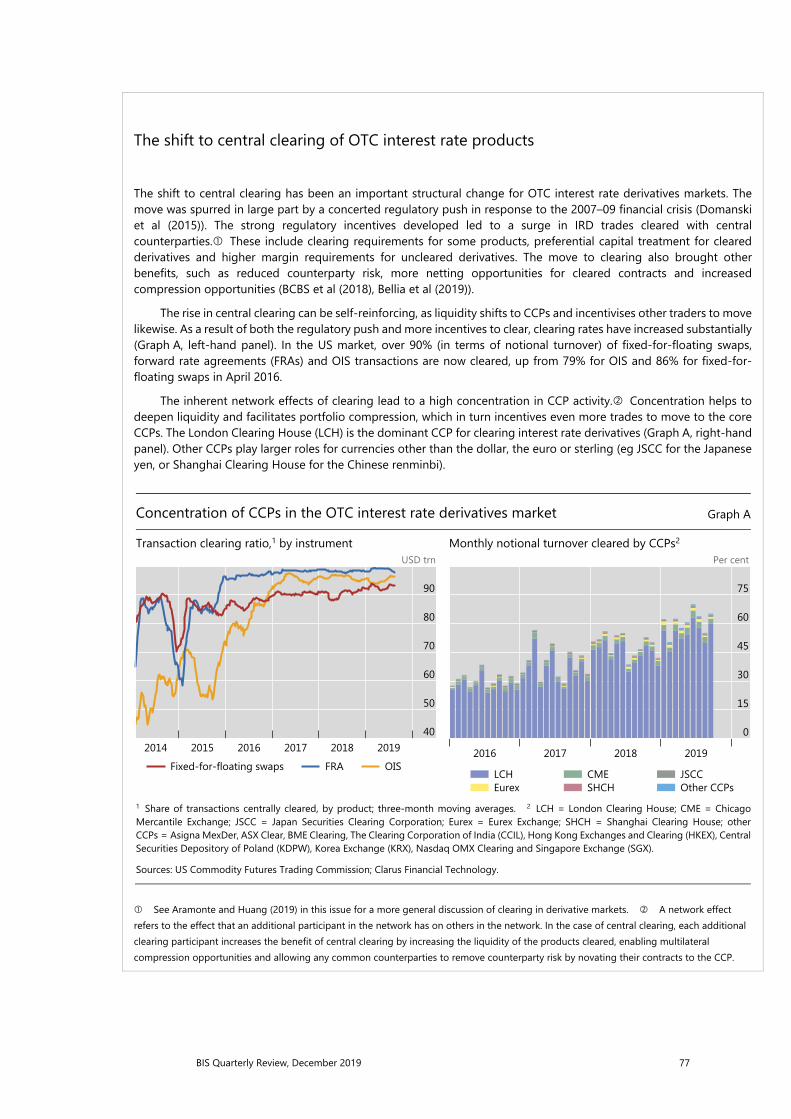
BIS Quarterly Review, December 2019 77
The shift to central clearing of OTC interest rate products
The shift to central clearing has been an important structural change for OTC interest rate derivatives markets. The move was spurred in large part by a concerted regulatory push in response to the 2007–09 financial crisis (Domanski et al (2015)). The strong regulatory incentives developed led to a surge in IRD trades cleared with central counterparties. These include clearing requirements for some products, preferential capital treatment for cleared derivatives and higher margin requirements for uncleared derivatives. The move to clearing also brought other benefits, such as reduced counterparty risk, more netting opportunities for cleared contracts and increased compression opportunities (BCBS et al (2018), Bellia et al (2019)).
The rise in central clearing can be self-reinforcing, as liquidity shifts to CCPs and incentivises other traders to move likewise. As a result of both the regulatory push and more incentives to clear, clearing rates have increased substantially (Graph A, left-hand panel). In the US market, over 90% (in terms of notional turnover) of fixed-for-floating swaps, forward rate agreements (FRAs) and OIS transactions are now cleared, up from 79% for OIS and 86% for fixed-for-floating swaps in April 2016.
The inherent network effects of clearing lead to a high concentration in CCP activity. Concentration helps to deepen liquidity and facilitates portfolio compression, which in turn incentives even more trades to move to the core CCPs. The London Clearing House (LCH) is the dominant CCP for clearing interest rate derivatives (Graph A, right-hand panel). Other CCPs play larger roles for currencies other than the dollar, the euro or sterling (eg JSCC for the Japanese yen, or Shanghai Clearing House for the Chinese renminbi).
Concentration of CCPs in the OTC interest rate derivatives market Graph A
Transaction clearing ratio,1 by instrument Monthly notional turnover cleared by CCPs2 USD trn Per cent
1 Share of transactions centrally cleared, by product; three-month moving averages. 2 LCH = London Clearing House; CME = ChicagoMercantile Exchange; JSCC = Japan Securities Clearing Corporation; Eurex = Eurex Exchange; SHCH = Shanghai Clearing House; other CCPs = Asigna MexDer, ASX Clear, BME Clearing, The Clearing Corporation of India (CCIL), Hong Kong Exchanges and Clearing (HKEX), CentralSecurities Depository of Poland (KDPW), Korea Exchange (KRX), Nasdaq OMX Clearing and Singapore Exchange (SGX). Sources: US Commodity Futures Trading Commission; Clarus Financial Technology.
See Aramonte and Huang (2019) in this issue for a more general discussion of clearing in derivative markets. A network effect refers to the effect that an additional participant in the network has on others in the network. In the case of central clearing, each additional clearing participant increases the benefit of central clearing by increasing the liquidity of the products cleared, enabling multilateral compression opportunities and allowing any common counterparties to remove counterparty risk by novating their contracts to the CCP.
90
80
70
60
50
40201920182017201620152014
Fixed-for-floating swaps FRA OIS
75
60
45
30
15
0
2019201820172016
LCHEurex
CMESHCH
JSCCOther CCPs
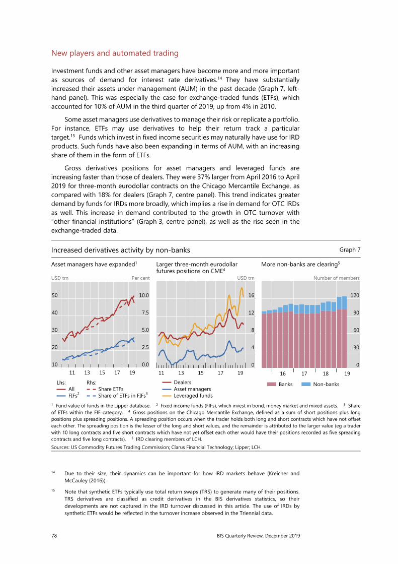
78 BIS Quarterly Review, December 2019
New players and automated trading
Investment funds and other asset managers have become more and more important as sources of demand for interest rate derivatives.14 They have substantially increased their assets under management (AUM) in the past decade (Graph 7, left-hand panel). This was especially the case for exchange-traded funds (ETFs), which accounted for 10% of AUM in the third quarter of 2019, up from 4% in 2010.
Some asset managers use derivatives to manage their risk or replicate a portfolio. For instance, ETFs may use derivatives to help their return track a particular target.15 Funds which invest in fixed income securities may naturally have use for IRD products. Such funds have also been expanding in terms of AUM, with an increasing share of them in the form of ETFs.
Gross derivatives positions for asset managers and leveraged funds are increasing faster than those of dealers. They were 37% larger from April 2016 to April 2019 for three-month eurodollar contracts on the Chicago Mercantile Exchange, as compared with 18% for dealers (Graph 7, centre panel). This trend indicates greater demand by funds for IRDs more broadly, which implies a rise in demand for OTC IRDs as well. This increase in demand contributed to the growth in OTC turnover with “other financial institutions” (Graph 3, centre panel), as well as the rise seen in the exchange-traded data.
14 Due to their size, their dynamics can be important for how IRD markets behave (Kreicher and
McCauley (2016)). 15 Note that synthetic ETFs typically use total return swaps (TRS) to generate many of their positions.
TRS derivatives are classified as credit derivatives in the BIS derivatives statistics, so their developments are not captured in the IRD turnover discussed in this article. The use of IRDs by synthetic ETFs would be reflected in the turnover increase observed in the Triennial data.
Increased derivatives activity by non-banks Graph 7
Asset managers have expanded1 Larger three-month eurodollar futures positions on CME4
More non-banks are clearing5
USD trn Per cent USD trn Number of members
1 Fund value of funds in the Lipper database. 2 Fixed income funds (FIFs), which invest in bond, money market and mixed assets. 3 Share of ETFs within the FIF category. 4 Gross positions on the Chicago Mercantile Exchange, defined as a sum of short positions plus longpositions plus spreading positions. A spreading position occurs when the trader holds both long and short contracts which have not offseteach other. The spreading position is the lesser of the long and short values, and the remainder is attributed to the larger value (eg a trader with 10 long contracts and five short contracts which have not yet offset each other would have their positions recorded as five spreading contracts and five long contracts). 5 IRD clearing members of LCH. Sources: US Commodity Futures Trading Commission; Clarus Financial Technology; Lipper; LCH.
50
40
30
20
10
10.0
7.5
5.0
2.5
0.01917151311
AllFIFs2
Lhs:Share ETFsShare of ETFs in FIFs3
Rhs:
16
12
8
4
01917151311
DealersAsset managersLeveraged funds
120
90
60
30
0
19181716
Banks Non-banks

BIS Quarterly Review, December 2019 79
Participation in central clearing highlights the importance of OTC IRD products for the overall strategies and business models of asset managers and other non-dealers. Many asset managers access CCP clearing services through affiliated banks or as clients to CCP members. Some non-banks have also started to directly clear their own positions by becoming clearing members with CCPs (Graph 7, right-hand panel). At end-March 2016, 96 bank members and five non-bank members cleared IRDs with LCH. By end-June 2019, the number of non-bank members jumped to 22 (with 102 bank members).
Another factor that bolstered the presence of asset managers and other new players in derivatives markets was a fall in transaction costs. Technological advances, including electronification, automation and algorithmic trading, have reduced these costs for trading in both OTC and exchange derivatives markets. They have also facilitated new investment strategies, in particular those using algorithmic trading.16
Automated trading has been on the rise across all derivatives markets in recent years. A trade is considered automated if it is “generated and/or routed without human intervention” (Haynes and Roberts (2015)).17 Its adoption has been steadily increasing on exchanges (Graph 8, left-hand panel). The implementation of swap execution facilities (SEFs) in the US (spurred in part by mandatory execution requirements for swap trades in the Dodd-Frank Act) indicates that automated trading is generally spreading through the OTC market as well (right-hand
16 Hedge funds and proprietary trading firms (PTFs) have led the increase in turnover in foreign
exchange OTC markets. PTFs often utilise centralised electronic trading platforms and algorithmic trading strategies. See Schrimpf and Sushko (2019b) in this issue for a discussion.
17 This is a broader set of trades than just those generated by algorithms, also including “those which are generated manually but make use of automated spreading functionality, or even those where manual traders use the order submission management of third-party trading systems” (Haynes and Roberts (2015)).
Automated trading has increased Graph 8
More automated trading for IRD futures1 Turnover with swap execution facilities rising2 Per cent USD bn
1 Futures contracts traded on the Chicago Mercantile Exchange. 14 = contracts executed between 12 November 2012 and 31 October 2014;16 = contracts executed between 1 November 2014 and 31 October 2016; 18 = contracts executed between 1 November 2016 and 31 October 2018. 2 Turnover with swap execution facilities in the United States. TW = Trade Web; other = BGC SEF, DW SEF, GFI Group, ICAP GlobalDerivatives Limited SEF (IGDL SEF), Javelin SEF, LatAm SEF, Tradition SEF and trueEX. Sources: Haynes and Roberts (2015, updated); Financial Industry Association.
100
75
50
25
0
US TreasurySTIRSIR deliverable swaps181614181614181614
Automated Manual Non-electronic
800
600
400
200
0
201920182017201620152014
Tullett PrebonTW
BloombergICAP
NEXOther
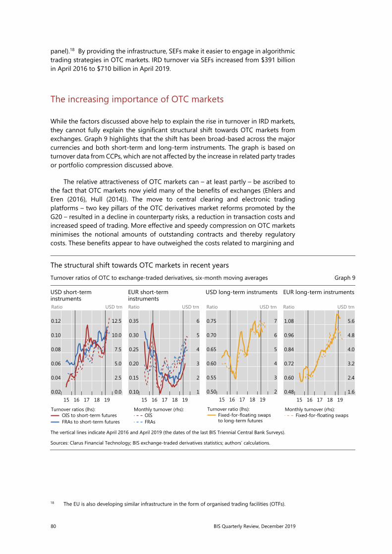
80 BIS Quarterly Review, December 2019
panel).18 By providing the infrastructure, SEFs make it easier to engage in algorithmic trading strategies in OTC markets. IRD turnover via SEFs increased from $391 billion in April 2016 to $710 billion in April 2019.
The increasing importance of OTC markets
While the factors discussed above help to explain the rise in turnover in IRD markets, they cannot fully explain the significant structural shift towards OTC markets from exchanges. Graph 9 highlights that the shift has been broad-based across the major currencies and both short-term and long-term instruments. The graph is based on turnover data from CCPs, which are not affected by the increase in related party trades or portfolio compression discussed above.
The relative attractiveness of OTC markets can – at least partly – be ascribed to the fact that OTC markets now yield many of the benefits of exchanges (Ehlers and Eren (2016), Hull (2014)). The move to central clearing and electronic trading platforms – two key pillars of the OTC derivatives market reforms promoted by the G20 – resulted in a decline in counterparty risks, a reduction in transaction costs and increased speed of trading. More effective and speedy compression on OTC markets minimises the notional amounts of outstanding contracts and thereby regulatory costs. These benefits appear to have outweighed the costs related to margining and
18 The EU is also developing similar infrastructure in the form of organised trading facilities (OTFs).
The structural shift towards OTC markets in recent years Turnover ratios of OTC to exchange-traded derivatives, six-month moving averages Graph 9
USD short-term instruments
EUR short-term instruments
USD long-term instruments EUR long-term instruments
Ratio USD trn Ratio USD trn Ratio USD trn Ratio USD trn
The vertical lines indicate April 2016 and April 2019 (the dates of the last BIS Triennial Central Bank Surveys). Sources: Clarus Financial Technology; BIS exchange-traded derivatives statistics; authors’ calculations.
0.12
0.10
0.08
0.06
0.04
0.02
12.5
10.0
7.5
5.0
2.5
0.01918171615
OIS to short-term futuresFRAs to short-term futures
Turnover ratios (lhs):
0.35
0.30
0.25
0.20
0.15
0.10
6
5
4
3
2
11918171615
OISFRAs
Monthly turnover (rhs):
0.75
0.70
0.65
0.60
0.55
0.50
7
6
5
4
3
21918171615
to long-term futuresFixed-for-floating swaps
Turnover ratio (lhs):
1.08
0.96
0.84
0.72
0.60
0.48
5.6
4.8
4.0
3.2
2.4
1.61918171615
Fixed-for-floating swapsMonthly turnover (rhs):
BIS Quarterly Review, December 2019 81
collateral requirements for cleared and uncleared derivatives, implemented in most jurisdictions including the United States and the European Union (FSB (2019)).
Exchanges have attempted to lure activity back from OTC markets by offering new instruments, such as swap futures. Zazzara (2019) dubs this the “futurisation of OTC markets”. While swap futures have been launched at various points in time, in part to capture increasing demand for longer-term IRDs referencing private benchmark rates (Kreicher et al (2017)), their success thus far has been limited. The dedicated futures exchange Eris, for instance, introduced a deliverable swap future in February 2013. Even though turnover in these contracts picked up in recent months as trading moved to CME in December 2018, it is still less than 0.5% of turnover in US dollar OTC swaps.
Conclusion
Turnover in interest rate derivatives markets has increased substantially over the last three years, particularly in OTC markets. A rise in non-market facing trades, such as compression and back-to-back trades, helped boost turnover in OTC markets. The change in the US monetary policy outlook and the move to shorter-maturity instruments also played a role. Further, continuing structural changes have been important in driving up IRD turnover, especially in OTC markets. Automated trading has expanded access and reduced transaction costs, as new players have moved into the market.
The regulatory push towards central clearing and electronic trading, as well as the evolution of compression services, has led to a relative shift from exchanges to OTC markets. OTC markets now offer many of the attractive features that exchanges held, while also maintaining a wider range of products and contracts and the ability to meet customised demands. These factors have led turnover growth in OTC markets to significantly outpace that in exchanges.
Looking forward, more structural changes may be on the horizon. The prospect of the United Kingdom leaving the European Union may influence the structure of OTC markets, especially with so much activity based in London. Moreover, the transition of benchmark rates to new overnight risk-free rates (RFRs) foreshadows significant changes in both the type of traded instruments and the relative importance of OTC versus exchange-traded markets. The range of derivative instruments will expand as debt contracts start to reference the new RFRs. Term benchmarks beyond overnight rates are needed to, for instance, determine interest obligations in cash instruments (eg bonds). Therefore, new instruments, such as OIS with RFRs as the floating rate or longer-term RFR futures, are likely to be developed. Depending on which instruments prevail, this could again shift trading between OTC markets and exchanges. Whether these new contracts will gain a significant market share or even replace existing ones is unclear, as multiple benchmarks may emerge to serve different purposes and fulfil different market needs (Schrimpf and Sushko (2019a)).

82 BIS Quarterly Review, December 2019
References
Aramonte, S and W Huang (2019): “OTC derivatives: euro exposures rise and central clearing advances”, BIS Quarterly Review, December, pp 83–93. Basel Committee on Banking Supervision, Financial Stability Board, Committee on Payments and Market Infrastructures and International Organization of Securities Commissions (2018): Incentives to centrally clear over-the-counter (OTC) derivatives: a post-implementation evaluation of the effects of the G20 financial regulatory reforms – final report, November. Bellia, M, G Girardi, R Panzica, L Pelizzon and T Peltonen (2019): “The demand for central clearing: to clear or not to clear, that is the question”, SAFE Working Paper, no 193, June. Domanski, D, L Gambacorta and C Picillo (2015): “Central clearing: trends and current issues”, BIS Quarterly Review, December, pp 59–76. Ehlers, T and E Eren (2016): “The changing shape of interest rate derivatives markets”, BIS Quarterly Review, December, pp 53–65. Financial Stability Board (2019): OTC derivatives market reforms: 2019 progress report on implementation, October. Gyntelberg, J and C Upper (2013): “The OTC interest rate derivatives market in 2013”, BIS Quarterly Review, December, pp 69–82. Haynes, R and J Roberts (2015): “Automated trading in futures markets”, white paper, Office of the Chief Economist, Commodity Futures Trading Commission. See also Update #1 and Update #2. Hull, J (2014): “The changing landscape for derivatives”, Journal of Financial Engineering, vol 1, no 3. Kreicher, L and R McCauley (2016): “Asset managers, eurodollars and unconventional monetary policy”, BIS Working Papers, no 578, August. Kreicher, L, R McCauley and P Wooldridge (2017): “The bond benchmark continues to tip to swaps”, BIS Quarterly Review, March, 69–79. Patel, N and D Xia (2019): “Offshore markets drive trading of emerging market currencies”, BIS Quarterly Review, December, pp 53–67. Schrimpf, A and V Sushko (2019a): “Beyond LIBOR: a primer on the new benchmark rates”, BIS Quarterly Review, March, pp 29–52. ——— (2019b): “Sizing up global foreign exchange markets”, BIS Quarterly Review, December, pp 21–37. Upper, C (2006): “Derivatives activity and monetary policy”, BIS Quarterly Review, September, pp 65–76. Zazzara, C (2019): “The new OTC derivatives landscape: (more) transparency, liquidity, and electronic trading”, Journal of Banking Regulation, pp 1–18, May.

BIS Quarterly Review, December 2019 83
OTC derivatives: euro exposures rise and central clearing advances1
The composition of amounts outstanding in over-the-counter derivatives shifted towards the euro and cleared instruments. Since the Great Financial Crisis, increases in central clearing rates have helped shape growth in amounts outstanding. Derivatives subject to regulatory clearing mandates were approaching full clearing, while clearing rates were low for certain products, including some with short maturities or liquid bilateral markets. JEL classification: G10; G18; G23.
Over-the-counter (OTC) markets are increasingly important for many types of derivative. This article examines how the composition of outstanding OTC derivatives has changed as they have become increasingly prevalent in financial markets. To explore the currency composition of outstanding OTC derivatives and trends in clearing, we draw on data from the combined BIS semiannual derivatives statistics and Triennial Central Bank Survey of OTC derivatives markets.2
The combined surveys show that interest rate derivatives still accounted for the largest share of the OTC derivatives recorded by dealers in advanced economies (AEs), while FX derivatives predominated in the outstanding positions of dealers from emerging market economies (EMEs). The euro’s share rose globally, accounting for 44% of AE dealers’ outstanding contracts by market value at end-June 2019, compared with 24% in US dollars. The euro became more relevant for dealers from emerging Europe in particular. Nevertheless, the US dollar remained the pre-eminent currency for EME dealers.
Since the Great Financial Crisis (GFC) of 2007–09, the dynamics of amounts outstanding in OTC derivatives markets have been shaped, in part, by regulatory reforms agreed at the 2009 G20 summit. Central clearing is a key element in authorities’ efforts to reform OTC derivatives markets and reduce systemic risk. The
1 The views expressed in this article are those of the authors and do not necessarily reflect those of the
Bank for International Settlements. We thank Kristina Micic for valuable assistance with the data. 2 Since 1998, the BIS has collected two sets of statistics on outstanding positions in OTC derivatives
markets: semiannual data from large derivatives dealers in 12 jurisdictions, and triennial data from smaller dealers in more than 30 jurisdictions. Both sets of data cover the worldwide consolidated positions of reporting dealers. According to the latest Triennial Survey, which captured positions at end-June 2019, smaller dealers accounted for about 8% of notional amounts outstanding (BIS (2019)). Between Triennial Surveys, the BIS uses the triennial data to scale up the semiannual data, thereby providing a more accurate estimate of the global size of OTC derivatives markets.
Sirio [email protected]
Wenqian Huang [email protected]

84 BIS Quarterly Review, December 2019
data on outstanding positions show that clearing rates increased substantially from 2010 to 2017. By 2019, contracts subject to mandatory clearing were cleared almost entirely by central counterparties (CCPs). 3 For OTC derivatives not subject to mandatory clearing, clearing rates varied across products, even though margin requirements incentivised central clearing.
The next section of this article discusses recent trends in outstanding positions. The second section focuses on clearing, and the final section concludes.
Trends across countries and currencies
The notional amount of OTC derivatives, which determines contractual payments, rose to $640 trillion at end-June 2019 (Graph 1, left-hand panel). This was its highest level since 2014, continuing an upward trend that started in 2015. Over the same period, the global sovereign and non-financial corporate bond markets expanded at a similar pace. The turnover of OTC derivatives rose even more rapidly than notional amounts, probably because (i) trade compression limited notional growth and (ii) turnover rose mainly for shorter-maturity instruments that are rolled over frequently (Ehlers and Hardy (2019) in this issue).
In contrast to the notional amount, gross market value, which is a better gauge of amounts at risk, has trended downward since 2012 (left-hand panel). It totalled about $12 trillion in mid-2019, compared with $15 trillion in mid-2015 and $26 trillion in mid-2012. Netting agreements reduced dealers’ credit exposure to $2.7 trillion at end-June 2019, equivalent to 22% of gross market value. In OTC derivatives markets, these credit exposures are typically covered by collateral.4
OTC derivatives referenced mainly interest rates. At end-June 2019, interest rate derivatives represented 73% of outstanding contracts by gross market value (Graph 1, right-hand panel). FX derivatives came a distant second, with 18%. Other derivatives, mostly in the form of equity and credit derivatives, accounted for 9% of gross market
3 The report of the Derivatives Assessment Team of the Financial Stability Board (FSB) recently found
that regulations provided impetus for central clearing (BCBS-CPMI-FSB-IOSCO (2018)). 4 In the BIS OTC derivatives statistics, gross credit exposure takes into account legally enforceable
bilateral netting agreements but not collateral. Gross credit exposure is reported only by dealers who participate in the semiannual survey.
Key takeaways
• The management of interest rate risk continued to dominate global OTC derivatives activity, although FX derivatives were more important among dealers from emerging market economies.
• Among dealers from emerging market economies, the share of interest rate derivatives cleared rose to the high levels reported by dealers from advanced economies.
• After increasing substantially following the GFC, clearing rates have levelled off recently, with mandated products approaching full clearing.

BIS Quarterly Review, December 2019 85
Global trends in OTC derivatives outstanding At half-year end Graph 1
Notional amounts outstanding (USD trillions) Gross market values (%)1
CD = credit derivatives; CO = commodity derivatives; EQ = equity-linked derivatives; FX = foreign exchange derivatives; IR = single-currency interest rate derivatives; OD = other derivatives. 1 As a percentage of the gross market value of all outstanding OTC derivatives. Source: BIS derivatives statistics.
30
24
18
12
6
0
700
560
420
280
140
0
1816141210080604020098
Gross market value (lhs) IRFX
100
80
60
40
20
0
1816141210080604020098
EQCD
ODCO
Composition of AE and EME dealers’ OTC derivatives exposure Share of gross market value of all outstanding OTC derivatives at end-June, in per cent Graph 2
By underlying risk Share of IRDs depending on debt securities market size1
Share of FX depending on FDI3
AED = advanced economy dealers (AT, AU, BE, CA, CH, DE, DK, ES, FI, FR, GB, GR, IE, IT, JP, LV, NL, NO, PT, SE and US); CD = credit derivatives; CO = commodity derivatives; EMD = emerging market dealers (ie dealers from countries that participate in the Triennial Survey, excluding those listed under AE); EQ = equity-linked derivatives; FDI = foreign direct investment; FX = foreign exchange derivatives; IR(Ds) = single-currency interest rate derivatives; OD = other derivatives. 1 Small (large) debt markets are countries whose share of debt securities markets in the total (ie global debt market estimate) is below (above) the median share. 2 Share in the total amount based on gross market values at end-June 2019. 3 The low (high) FDI categories includecountries whose foreign direct investment as a share of GDP is below (above) the median. As at December 2018. 4 Share in the total amount based on gross market values at end-June 2019. Sources: Dealogic; Euroclear; Thomson Reuters; Xtrakter Ltd; World Bank; national data; BIS derivatives statistics; BIS calculations; authors’ calculations.
100
80
60
40
20
0EMDAEDEMDAED
2016 2019
IRFX
EQCO
CDOD
70
56
42
28
14
0Large debt marketsSmall debt markets
Median share of IRDs2
40
32
24
16
8
0High FDILow FDI
Median share of FX4

86 BIS Quarterly Review, December 2019
value. For AE dealers, exposures were concentrated in interest rate derivatives (74%); for EME dealers, they were mainly in FX derivatives (57%) (Graph 2, left-hand panel).5
Differences in exposures reported by AE and EME dealers reflected structural economic differences across countries. In particular, exposure to interest rate derivatives was higher for dealers from countries with larger debt securities markets, while FX derivatives were more significant for dealers from countries receiving relatively more foreign direct investment (Graph 2, centre and right-hand panels). The balance sheet composition of AE and EME dealers also differed in terms of currencies. AE dealers reported that their exposures consisted mainly of derivatives referencing the euro and the US dollar: 44% and 24%, respectively, at end-June 2019. For EME dealers, the US dollar was the key reference currency, representing 41% of their exposures (Graph 3, left-hand panel).
The euro’s share of outstanding market value has increased appreciably over the past three years. Among dealers from AEs, the share of euro-denominated derivatives increased by 6 percentage points from 38% at end-June 2016. Over the same period, the share of euro-denominated derivatives in market value terms rose by 6 percentage points in EMEs, from 2% in 2016 to 8% in 2019. Dealers in emerging Europe drove the increase in euro exposure for EME dealers. While the share of euro-denominated OTC derivatives rose for euro area dealers and those in other AEs, it was considerably more pronounced for dealers in emerging Europe (Graph 3, centre panel).
5 In the following discussion, exposures are defined in terms of gross market value. For comparisons
of AE and EME derivatives markets in terms of size, instrument type and currencies, see eg Patel and Xia (2019), Upper and Valli (2016) and Wooldridge and Xia (2019).
Euro share expands, especially in FX derivatives Gross market values Graph 3
By currency and dealers1 Euro-denominated OTC derivatives2 By currency and market risk category3
Per cent USD trn
AED = advanced economy dealers (AT, AU, BE, CA, CH, DE, DK, ES, FI, FR, GB, GR, IE, IT, JP, LV, NL, NO, PT, SE and US); AE (other) = advancedeconomies excluding euro area economies; EM Asia = developing Asia and Pacific (see EMEs); EMD = emerging market dealers (ie those fromcountries that participate in the Triennial Survey excluding AEs); EM Europe = developing Europe (see EMD); FX = foreign exchange derivatives; IRDs = single-currency interest rate derivatives. 1 Interest rate and foreign exchange derivatives only. As at end-June. 2 The share of euro-denominated interest rate and foreign exchangederivatives in the total of all currencies. As at end-June. 3 Dealers headquartered in AEs only. As at half-year end. Source: BIS derivatives statistics.
100
80
60
40
20
0EMDAEDEMDAED
2016 2019
USDEUR
GBPJPY
other
Euro area
AE (other)
EM Europe
Euro area
AE (other)
EM Europe
EM Asia
71
56
41
26
11
7564534231209
FX IRDs2016 (%)
2019
(%)
10
8
6
4
2
0
19171513110907050301
USDEUR
IRD: USDEUR
FX:

BIS Quarterly Review, December 2019 87
A further breakdown of dealers’ currency exposures by asset class shows that the US dollar dominated FX derivatives, while the euro surpassed other currencies in interest rate derivatives. In the latter case, euro and US dollar exposures were roughly similar until end-2011, when a gap opened rapidly, only stabilising after end-2014 (Graph 3, right-hand panel). The opening of this gap coincided with the ECB’s introduction of longer-term refinancing operations to support bank lending and liquidity in the euro area money market.
In addition to hedging portfolio currency risk, FX swaps are used to cover US dollar financing needs, for both financial institutions (Baba and Packer (2009)) and non-financial corporates (Borio et al (2017)). In recent years, banks’ use of FX swaps to manage funding liquidity has also increased (Schrimpf and Sushko (2019)).
Central clearing shaped patterns in derivatives outstanding
Rising central clearing rates, spurred by the post-crisis regulatory framework agreed at the 2009 G20 summit, have shaped the evolution of outstanding derivatives amounts since the GFC. This section reviews broad central clearing trends, highlights key channels through which central clearing can affect outstanding derivatives amounts and discusses central clearing rates in key market segments in the light of regulatory initiatives.
Clearing rates levelled off overall, rose for EME dealers
There were marked differences in central clearing rates across derivative types.6 For interest rate and credit derivatives, substantial increases in the early years after the GFC levelled off recently. In particular, clearing rates rose from 55% in 2010 to 75% in 2017 for interest rate derivatives. Over the same period, the increase for credit default swaps (CDS) was also remarkable, from 10% to 55%. However, clearing rates barely inched up between 2018 and 2019 (Graph 4, left-hand panel).
For FX derivatives, the share of notional amounts for which CCPs are dealer counterparties was just 4% at end-June 2019 (right-hand panel). Low clearing rates for FX derivatives probably reflected the fact that most of these derivatives are deliverable contracts, which are not particularly suited for central clearing because they involve the exchange of notional principal, thus requiring CCPs with large balance sheets and access to funding in multiple currencies.
The clearing rates of EME dealers caught up with those of AE dealers over the past three years. AE dealers generally reported higher rates than those from EMEs and were approaching full clearing, while rates increased substantially for EME dealers (Graph 5, left-hand panel). AE currencies had higher clearing rates, while EME ones exhibited more substantial growth in central clearing (right-hand panel).
6 The proportion of outstanding positions against CCPs is typically larger than the proportion of trades
cleared through CCPs because the former counts trades between dealers twice. In the BIS OTC derivatives statistics, whereas inter-dealer positions are adjusted to eliminate double-counting, inter-dealer trades that are subsequently novated to a CCP are not adjusted. For further discussion, see Wooldridge (2016).

88 BIS Quarterly Review, December 2019
Central clearing advances after the Great Financial Crisis Notional amounts outstanding Graph 4
Clearing rates1 Notional amounts outstanding,2 by counterparty and underlying risk
Per cent Per cent
CD = credit derivatives; CDS = credit default swaps; IRDs = interest rate derivatives; other = foreign exchange and equity derivatives. 1 Calculated as a share of notional amounts outstanding reported vis-à-vis CCPs in the total notional amounts outstanding. For IRDs, datafor CCPs prior to end-June 2016 are estimated by indexing the amounts reported at end-June 2016 to the growth since 2008 of notional amounts outstanding cleared through LCH’s SwapClear service. At half-year end. 2 As a percentage of the notional amount of alloutstanding OTC derivatives. As of end-June. 3 Contracts between reporting dealers that are subsequently novated to CCPs are recordedtwice. 4 Excluding central counterparties and reporting dealers. Sources: LCH.Clearnet Group Ltd; BIS derivatives statistics.
Rising clearing rates can reduce outstanding notional and gross market value in three main ways. First, offsetting positions can be netted across multiple parties. Second, CCPs have a complete view of the positions of their clearing members, facilitating trade compression.7 Since the clearing mandate took effect in 2012, the notional amount of compression trades increased substantially (Ehlers and Hardy (2019) in this issue). Third, central clearing allows settled-to-market (STM), in which traders take ownership of variation margins and the market value of the derivatives is reset to zero frequently. Some dealer banks indicated that gross derivatives market value in their public reporting dropped because of STM.8
Clearing rates for mandated versus non-mandated contracts
In the aftermath of the GFC, regulatory initiatives promoting central clearing were two-pronged. First, central clearing was mandated for a set of standardised contracts – including forward rate agreements (FRAs), interest rate swaps (IRS) and CDS indices. Second, uncleared contracts were to face higher capital and margin requirements, primarily to better reflect their risk profiles but also to promote central clearing.
7 Compression is a process whereby two or more counterparties tear up existing derivatives contracts
and replace them with a smaller number of new ones that leave the economic exposures materially unchanged. The elimination of economically redundant derivatives positions reduces the number of contracts and gross notional amounts.
8 See eg the annual reports of Goldman Sachs (2016) and Wells Fargo (2017).
80
64
48
32
16
0191715131109
IRDs CDS
100
80
60
40
20
0OtherCDIRDsOtherCDIRDs
2016 2019Central counterparties3
Other financial institutions4
Non-financial customersReporting dealers
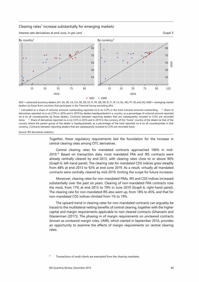
BIS Quarterly Review, December 2019 89
Together, these regulatory requirements laid the foundation for the increase in central clearing rates among OTC derivatives.
Central clearing rates for mandated contracts approached 100% in mid-2019. 9 Based on transaction data, most mandated FRA and IRS contracts were already centrally cleared by end-2013, with clearing rates close to or above 90% (Graph 6, left-hand panel). The clearing rate for mandated CDS indices grew steadily from 48% at end-2013 to 92% at end-June 2019. As a result, virtually all mandated contracts were centrally cleared by mid-2019, limiting the scope for future increases.
Moreover, clearing rates for non-mandated FRAs, IRS and CDS indices increased substantially over the past six years. Clearing of non-mandated FRA contracts rose the most, from 17% at end-2013 to 79% in June 2019 (Graph 6, right-hand panel). The clearing rate for non-mandated IRS also went up, from 18% to 45%, and that for non-mandated CDS indices climbed from 1% to 19%.
The upward trend in clearing rates for non-mandated contracts can arguably be traced to the multilateral netting benefits of central clearing, together with the higher capital and margin requirements applicable to non-cleared contracts (Ghamami and Glasserman (2017)). The phasing-in of margin requirements on uncleared contracts (known as uncleared margin rules, UMR), which started in September 2016, provides an opportunity to examine the effects of margin requirements on central clearing rates.
9 Transactions of small clients are exempted from the clearing mandates.
Clearing rates1 increase substantially for emerging markets Interest rate derivatives at end-June, in per cent Graph 5
By country2 By currency3
AED = advanced economy dealers (AT, AU, BE, CA, CH, DE, DK, ES, FI, FR, GB, GR, IE, IT, JP, LV, NL, NO, PT, SE and US); EMD = emerging market dealers (ie those from countries that participate in the Triennial Survey excluding AEs). 1 Calculated as a share of notional amounts outstanding reported vis-à-vis CCPs in the total notional amounts outstanding. 2 Share of derivatives reported vis-à-vis CCPs in 2016 and in 2019 by dealers headquartered in a country, as a percentage of notional amount reportedvis-à-vis all counterparties by those dealers. Contracts between reporting dealers that are subsequently novated to CCPs are recorded twice. 3 Share of derivatives reported vis-à-vis CCPs in 2016 and in 2019 in the currency of the “home” country of the dealer (ie that of thecountry where the parent group of the dealer is headquartered), as a percentage of the total reported vis-à-vis all counterparties in that currency. Contracts between reporting dealers that are subsequently novated to CCPs are recorded twice. Source: BIS derivatives statistics.
95
75
55
35
15
9575553515
AED2016
95
75
55
35
15
1159575553515
EMD2016
2019

90 BIS Quarterly Review, December 2019
Margin requirements rose markedly after UMR were implemented. They were first applied to financial firms with month-end notional derivatives exposure greater than €3 trillion (“phase 1 firms”), followed by firms with smaller notional exposure.10 UMR led to significantly higher margin requirements, with phase 1 firms collecting $84 billion and posting $83 billion in initial margin at end-2018 for non-centrally cleared derivatives subject to UMR (Graph 7, left-hand panel). These figures were roughly 80% higher than in March 2017 and represented about 40% of total initial margins with CCPs for interest rate and credit derivatives.
We can gauge the impact of UMR on central clearing by linking the staggered implementation of UMR to the evolution of clearing rate differences between products subject to early or late UMR implementation. In particular, phase 1 firms in Japan and the United States were required to post margin from 1 September 2016, while those in the European Union had to do so only after 1 February 2017.
Our analysis suggests that UMR incentivised central clearing for non-deliverable forwards (NDFs) and non-mandated CDS.11 For both products, traders in the US dollar- and Japanese yen-denominated segments moved to central clearing in the run-up to 1 September 2016, while those in the euro-denominated segment migrated gradually between late 2016 and early 2017. As a result, the clearing rates of the dollar-/yen-denominated and euro-denominated segments diverged just before the first implementation deadline and converged again as the second deadline approached (Graph 7, centre and right-hand panels).
Although post-crisis regulatory reforms promoted central clearing, clearing rates for non-mandated contracts remained low for some products. The box discusses why central clearing became common for some products but not for others. Since moving from bilateral to central clearing can be costly, migration takes place only if there are
10 Physically delivered FX derivatives and small entities are exempted. 11 We focus on NDFs and non-mandated CDS because they are representative of relatively simple
products that can potentially be centrally cleared.
Clearing rates1 for mandated and non-mandated contracts Transactions, monthly data, in per cent Graph 6
Mandated contracts Non-mandated contracts
1 Calculated as a share of notional amounts traded vis-à-vis CCPs in total notional amounts traded. 2 Includes basis swaps, OIS and fixed/floating swaps. 3 CDS index. Sources: Depository Trust and Clearing Corporation Swap Data Repository; authors’ calculations.
90
70
50
30
10
201920182017201620152014
Forward rate agreementsInterest rate swaps2
Multi-name credit default swaps3
90
70
50
30
10
201920182017201620152014
SwaptionForeign exchange optionsNon-deliverable forwards

BIS Quarterly Review, December 2019 91
substantial net benefits from central clearing. All else equal, migration is less likely for products with more modest netting benefits, such as those with shorter maturity. Likewise, higher liquidity in the bilateral segment can increase the costs of switching to central clearing.
Conclusion
In recent years, the composition of outstanding OTC derivatives has shifted. First, the Triennial Survey shows that balance sheet composition differed considerably across AE and EME dealers. In terms of market value outstanding, exposure was mostly to interest rate derivatives for AE dealers and to FX derivatives for EME dealers. As for currencies, exposure was mostly to the US dollar for EME dealers and more evenly split between the euro and the US dollar for AE dealers. With significant US dollar credit to EMEs (McCauley et al (2015)), FX derivatives referencing the US dollar could be used to hedge currency risk, but could also be a source of US dollar financing (Borio et al (2017)).
Second, the euro made inroads globally. In particular, its share of outstanding market value rose in interest rate derivatives for AE dealers and in FX for EME dealers. As has been the case since end-2011, the euro overshadowed other currencies in terms of market value for interest rate derivatives reported by AE dealers.
Last but not least, central clearing rates increased in EMEs but grew less quickly overall, as mandated contracts approached full clearing. As a natural result of the regulatory reforms spurred by the 2009 G20 summit, the prominent role of CCPs makes their resilience and appropriate recovery and resolution planning essential for financial stability (BCBS-CPMI-FSB-IOSCO (2017)).
Margin requirements for uncleared trades incentivised central clearing Graph 7
Initial margin NDFs2 ` Non-mandated CDS2 USD bn Per cent Per cent
1 The regulatory initial margin (IM) is the margin pledged by 20 phase 1 financial firms that are surveyed by the ISDA. 2 The difference in the clearing rates between the USD/JPY and the EUR segments, where the clearing rate is defined as the share of notional amounts outstanding reported vis-à-vis CCPs in the total notional amounts outstanding subject to margin requirements (ie the fully collateralisedsegment). Sources: Clarus Financial Technology; Depository Trust and Clearing Corporation Swap Data Repository; International Swaps and DerivativesAssociation (ISDA); authors’ calculations.
200
150
100
50
0
2019201820172016
CCP IM ReceivedPosted
Regulatory IM:1
20
16
12
8
4
0
Q2 17Q4 16Q2 16
firmsphase 1 US & JP Sep 16
firmsphase 1EUFeb 17
Difference
80
70
60
50
40
30
Q2 17Q4 16Q2 16
firmsphase 1 US & JP Sep 16
firmsphase 1EUFeb 17
Average

92 BIS Quarterly Review, December 2019
Costs and benefits of switching to central clearing Why did trading in some derivatives migrate to central clearing, while staying with bilateral clearing for others? Among derivatives not subject to mandatory clearing, the rate of voluntary clearing differed substantially. In particular, the clearing rate for non-deliverable forwards (NDFs) was much lower than that for non-mandated credit default swaps (CDS). Such divergence can be explained, in part, by structural differences across the two products.
A substantial share of CDS trading has moved to central clearing over time, even in the absence of an official requirement. In June 2019, the monthly volume of centrally cleared CDS was, at $15 billion, comparable with the $23 billion of CDS that was cleared bilaterally each month (Graph A, left-hand panel). In comparison, the monthly volume of bilaterally cleared NDFs stood at $975 billion in June 2019, dwarfing that of centrally cleared NDFs (centre panel).
The decision to switch from bilateral to central clearing depends on a cost-benefit analysis that takes account of several elements. Among the potential benefits, lower capital or margin requirements certainly play a role, but so does the comparative ease of trade, or trading liquidity, in the bilaterally cleared and centrally cleared venues. These benefits vary across products, meaning that migration to central clearing might be cost-effective for some but not for others.
Structure and liquidity of two major non-mandated contracts1 Graph A
Non-mandated CDS NDFs Illiquidity measure2 for NDFs USD bn USD bn
1 Only DTCC trades that are subject to the margin requirement for uncleared trades, ie trades that are fully collateralised including centrallycleared trades and bilaterally cleared but fully collateralised ones. 2 Log Amihud illiquidity measure. Sources: Amihud (2002); Depository Trust and Clearing Corporation (DTCC) Swap Data Repository; authors’ calculations.
First, gains from margin netting in central clearing are higher if similar products are subject to clearing mandates. The reason is that CCPs generally allow for netting within the same asset class and initial margin is calculated at the portfolio level. Unlike NDFs, standardised CDS contracts are subject to the central clearing mandate, and non-mandated CDS can benefit from margin netting under central clearing.
Second, CDS generally have longer maturities than NDFs. Maturity is a key determinant of margin requirements for uncleared products. It is often less than one year for NDFs and typically five years for CDS. All else equal, the longer the maturity, the higher the margin requirement. Given the multilateral netting benefits of central clearing, the potential for margin reduction is greater for CDS than for NDFs.
Third, significantly lower liquidity in centrally cleared markets can reduce the incentive to switch away from bilaterally cleared venues. Coordination among traders plays an important role in this instance, because liquidity in centrally cleared markets could improve rapidly if enough traders opted out of bilateral clearing at the same time. Such coordination can be difficult to achieve when other advantages from switching, such as gains from netting, are small. For NDFs, the relatively small margin netting benefits provided little incentive for enough traders to migrate, and liquidity remained concentrated in bilaterally cleared markets, further discouraging migration to centrally cleared venues (Graph A, right-hand panel). For a discussion of the effect of counterparty credit risk on traders’ decisions to clear through CCPs rather than bilaterally, see P Fiedor, “Clearinghouse-Five: determinants of voluntary clearing in European derivatives markets”, European Systemic Risk Board, ESRB Working Paper Series, no 72, March 2018; M Bellia, R Panzica, L Pelizzon and T Peltonen, “The demand for central clearing: to clear or not to clear, that is the question”, European Systemic Risk Board, ESRB Working Paper Series, no 62, December 2017.
60
48
36
24
12
0
2019201820172016
CentrallyCleared:
1,000
800
600
400
200
0
2019201820172016
Bilaterally
–10
–15
–20
–25
–30
–35–5–10–15–20–25
Centrally cleared
Bila
tera
lly c
lear
ed

BIS Quarterly Review, December 2019 93
References
Amihud, Y (2002): “Illiquidity and stock returns: cross-section and time-series effects”, Journal of Financial Markets, vol 5, no 1, pp 31–56. Baba, N and F Packer (2009): “Interpreting deviations from covered interest parity during the financial market turmoil of 2007–08”, Journal of Banking & Finance, vol 33, no 11, pp 1953–62. Bank for International Settlements (2019): “OTC derivatives statistics at end-June 2019”, Statistical release, pp 1–8. Basel Committee on Banking Supervision, Committee on Payments and Market Infrastructures, Financial Stability Board and International Organization of Securities Commissions (2017): Chairs’ report on the implementation of the joint workplan for strengthening the resilience, recovery and resolvability of central counterparties, July. ——— (2018): Incentives to centrally clear over-the-counter (OTC) derivatives: a post-implementation evaluation of the effects of the G20 financial regulatory reforms – final report, November. Borio, C, R McCauley and P McGuire (2017): “FX swaps and forwards: missing global debt?”, BIS Quarterly Review, September, pp 37–54. Ehlers, T and B Hardy (2019): “The evolution of OTC interest rate derivatives markets”, BIS Quarterly Review, December, pp 69–82. Financial Stability Board (2018): OTC derivatives markets reforms: thirteenth progress report on implementation, August. Ghamami, S and P Glasserman (2017): “Does OTC derivatives reform incentivize central clearing?”, Journal of Financial Intermediation, vol 32, pp 76–87. Goldman Sachs (2016): Annual Report, pp 131–2. McCauley, R, P McGuire and V Sushko (2015): “Dollar credit to emerging market economies”, BIS Quarterly Review, December, pp 27–41. Patel, N and D Xia (2019): “Offshore markets drive trading of emerging market currencies”, BIS Quarterly Review, December, pp 53–67. Schrimpf, A and V Sushko (2019): “Sizing up global foreign exchange markets”, BIS Quarterly Review, December, pp 21–38. Upper, C and M Valli (2016): “Emerging derivatives markets?”, BIS Quarterly Review, December, pp 67–80. Wells Fargo (2017): Annual Report, p 154. Wooldridge, P (2016): “Central clearing predominates in OTC interest rate derivatives markets”, BIS Quarterly Review, December, pp 22–4. Wooldridge, P and D Xia (2019): “Derivatives trading in OTC markets soars”, BIS Quarterly Review, September, pp 32–3.


BIS Quarterly Review, December 2019 95
Euro repo market functioning: collateral is king1
Repo markets play a major role in redistributing liquidity and collateral between financial institutions. A unique transaction-level database reveals how the euro-denominated repo market has performed since the mid-2000s. We find that the market recovered strongly from periods of intense stress, even though it remains segmented according to the home country of the collateral used. In recent years, signs of segmentation have increased as the main motivation of repo market participants has shifted from funding to the trading of collateral. JEL classification: E40, E58, G15, G23.
As a key component of the money market, the repo market is a major channel for circulating cash and collateral through the financial system. Since the mid-2000s, repos have grown to become the predominant source of short-term funding in euro-denominated markets. In this period, the market has weathered stress during the Great Financial Crisis (GFC) of 2007–09 and the European sovereign debt crisis of 2011–12, and has coped with changes such as the ECB’s introduction of unconventional monetary policy and the advent of new financial sector regulation. This article tracks the repo market’s functioning in the face of these developments.
We use a unique transaction-level data set for centrally cleared euro-denominated repos to examine the market’s liquidity and pricing efficiency. We find signs that the market is persistently segmented according to the home country of the collateral used. This may impede the redistribution of liquidity. Yet, despite this segmentation, we find that the repo market remained functional during periods of stress: transaction costs stayed low and prices themselves adjusted smoothly to changing fundamentals.
We also find increasing signs that, in recent years, the market has been driven by investors in search of specific collateral rather than investors seeking funding. This feature has strengthened segmentation along collateral lines. Consistent with segmentation, individual participants have “preferred habitats”, in the sense of systematically borrowing and lending against collateral of a given country.
The following section outlines trading activity in the euro repo market over the 2006–18 period. We then discuss how different segments performed in terms of
1 The authors thank Claudio Borio, Stijn Claessens, Jörg Diener, Andreas Schrimpf, Egon Zakrajšek and,
especially, Philip Wooldridge for helpful comments and suggestions. The views expressed in this article are those of the authors and do not necessarily reflect those of the Bank for International Settlements.
Patrick [email protected]
Angelo [email protected]
Kostas [email protected]

96 BIS Quarterly Review, December 2019
liquidity and pricing efficiency. The third and fourth sections examine the intensity of arbitrage trades across segments and the tendency of market participants to specialise in individual collateral segments. The final section concludes.
Trends in transaction volumes
A repurchase agreement (repo) is a two-legged transaction that resembles a collateralised loan. A borrower of cash sells securities (the collateral) to the lender and agrees to buy them back later at a pre-specified price.2 Typical borrowers of cash are asset managers, pension funds and insurance companies. Typical lenders of cash are money market funds and corporate treasurers. Repos are intermediated by large broker-dealers, who are also significant repo users in their own right, to finance market-making inventory, source short-term funding or invest cash. Repo transactions can be either bilateral trades or cleared through a central counterparty.3
Repo markets fulfil two key functions. The first is to facilitate the borrowing and lending of cash. Repos are an attractive option for lenders seeking to place cash, because the collateral they receive (including haircuts and margin calls) mitigates credit risk. The second function is to facilitate the circulation of collateral or the exchange (swap) of collateral. Lenders of cash can obtain specific securities (for speculation, to cover short positions etc) for the repo’s duration, while lenders of the securities improve their portfolio liquidity without an outright sale.
These two functions represent the main motivations for investor participation in the repo market: the search for funding and the search for collateral. They are also roughly echoed in the two main market segments: general collateral (GC) repos and specific collateral (SC) repos. In the GC segment, the borrowing and lending of cash is the primary motivation for the transaction, the only requirement for the underlying collateral being that it offers sufficient credit quality. The SC segment is better suited to trades driven by collateral needs, because transactions specify the particular security that is exchanged in the two legs (Mancini et al (2016)).
The outstanding volume of euro-denominated repos exceeded €500 billion at end-2018. In the absence of comprehensive data on the euro repo market, our analysis focuses on cleared trades. Our database pools transaction data from three electronic platforms: BrokerTec, Eurex Repo and MTS Repo. These platforms cover
2 A repo transaction from the point of view of the seller of the securities is a reverse repo when seen
from the point of view of the lender (the buyer of the securities). 3 We classify tri-party repos as bilateral since credit risk remains between buyer and seller.
Key takeaways
• The euro repo market is a key channel for redistributing liquidity between financial institutions. • The market shows signs of persistent segmentation according to the home country of the collateral. • In recent years, demand for collateral has replaced funding considerations as the main driver of activity,
further emphasising segmentation.

BIS Quarterly Review, December 2019 97
the near-universe of centrally cleared repos denominated in euros, which in turn account for more than two thirds of overall activity (ECB (2015)). To analyse potential differences across segments, we consider only transactions using German, French, Italian or Spanish government bonds as collateral (SC and GC), as well as those using the GC Pooling basket, which encompasses securities eligible as collateral in the ECB’s framework. This results in nine collateral segments, which account for more than 75% of the centrally cleared market and about 50% of the total market.4 Thus, our sample is broadly representative of the overall market.
The euro repo market has grown significantly since the mid-2000s. Graph 1 shows the daily trading volumes for each collateral segment between 2006 and 2018.5 The total volume of transactions in our data increased from about €200 billion in late 2011 to about €300 billion in late 2018. This growth has been most evident in the Italian and Spanish collateral segments, especially in SC, even when activity in the German segment slowed, as in late 2011.6 Below we discuss other patterns of differential dynamics across collateral segments.
One feature of the market that comes through clearly in Graph 1 is the preference of traders for specific over general collateral. Turnover has been significantly higher in SC segments than in GC segments, and trends in the two
4 We cover repos with a one-day maturity (overnight, tomorrow-next, spot-next). These make up 95%
of centrally cleared transactions. Over 75% of repos with one-day maturity are centrally cleared. We use figures in ECB (2015) to compute market shares.
5 The trading volume of a given segment equals the nominal amount of the cash leg of transactions settled on that day against the collateral and contract type that define the segment. Repo dynamics depend on when cash and collateral are exchanged, rather than when the repo was negotiated.
6 As data from MTS Repo are available from 2010, our sample includes repos against Italian collateral only from 2010 onwards.
Trading activity Turnover,1 in billions of euros Graph 1
Specific collateral General collateral
The vertical lines indicate 15 October 2008 (switch to fixed rate full allotment), 21 December 2011 (LTRO), 9 March 2015 (PSPP) and 19 January2017 (relaxation of eligibility requirements). Data from MTS Repo – which handles most of the Italian repos – are only available from 2010 onwards. 1 Nominal amount of the cash leg of transactions settled on that day against the collateral and contract type that define the segment. Sources: BrokerTec; Eurex Repo; MTS Repo; authors’ calculations.
250
200
150
100
50
0
18161412100806
Germany France Italy
250
200
150
100
50
0
18161412100806
Spain GC pool

98 BIS Quarterly Review, December 2019
segments have diverged after 2015. Indeed, in 2015–18, turnover in the SC segment almost doubled, to €250 billion, whereas that in GC halved, to €50 billion. This divergence is consistent with a shift in the euro repo market towards transactions that are more securities-driven and less funding-driven (Brand et al (2019)).
The trends in market activity since the GFC are linked to the conduct of monetary policy. In late 2011, trading volumes dropped temporarily after the ECB introduced its longer-term refinancing operations (LTRO), which gave banks an alternative source of liquidity. In March 2015, turnover dropped after the ECB started to buy government bonds under its public sector purchase programme (PSPP). Collateral scarcity from the central bank’s purchases boosted activity in SC segments and reduced it in GC segments (especially the GC pool).7 SC segments received a further boost around the end of 2016, when the ECB enhanced its Securities Lending Programme (SLP) and relaxed the rules for eligible securities.
Liquidity and pricing efficiency
In a well functioning market, prices adjust promptly to shifts in underlying economic drivers, and do so smoothly. In this section, we analyse metrics of liquidity and pricing efficiency for the various collateral segments of the euro repo market. The metrics confirm the differences in the behaviour of these segments and point to the enhanced importance of collateral demand as a driver of the euro repo market.
Market liquidity
Liquidity generally refers to the market’s capacity to smoothly absorb traders’ orders (CGFS (1999)). We consider two measures of market liquidity: the effective spread and the price impact (see box). The effective spread uses the covariance between price changes in successive transactions to gauge the (unobserved) effective bid-ask spread. Transaction costs, such as the effective spread, are low in liquid markets. The price impact is calculated as the ratio of price changes to trading volume, with a low value indicating a liquid market. We use the repo rate as the relevant price.
Liquidity in the euro repo market was high on average over the period, but deteriorated at times in response to specific factors. Effective spreads were generally low, between 1 and 3 basis points (Graph 2, top panels), and so too was the price impact of trades, usually remaining below 10 basis points per billion euros in transaction volume (bottom panels). However, indicators across all segments deteriorated markedly but to varying extents in 2010–11 during the European sovereign debt crisis. They improved after the LTRO made its debut in December 2011. The introduction of the PSPP in 2015 had a moderately negative impact on repo liquidity, although its influence is confounded by the phasing-in of regulatory reforms that increased the capital requirement for banks’ repo market activities, lifting banks’
7 The effect of ECB purchases on bond scarcity came on top of higher demand from banks for high-
quality liquid assets, which was related to changes in liquidity regulations.
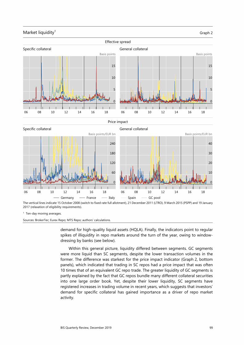
BIS Quarterly Review, December 2019 99
demand for high-quality liquid assets (HQLA). Finally, the indicators point to regular spikes of illiquidity in repo markets around the turn of the year, owing to window-dressing by banks (see below).
Within this general picture, liquidity differed between segments. GC segments were more liquid than SC segments, despite the lower transaction volumes in the former. The difference was starkest for the price impact indicator (Graph 2, bottom panels), which indicated that trading in SC repos had a price impact that was often 10 times that of an equivalent GC repo trade. The greater liquidity of GC segments is partly explained by the fact that GC repos bundle many different collateral securities into one large order book. Yet, despite their lower liquidity, SC segments have registered increases in trading volume in recent years, which suggests that investors’ demand for specific collateral has gained importance as a driver of repo market activity.
Market liquidity1 Graph 2
Effective spread Specific collateral General collateral
Basis points Basis points
Price impact
Specific collateral General collateral Basis points/EUR bn Basis points/EUR bn
The vertical lines indicate 15 October 2008 (switch to fixed rate full allotment), 21 December 2011 (LTRO), 9 March 2015 (PSPP) and 19 January2017 (relaxation of eligibility requirements). 1 Ten-day moving averages.
Sources: BrokerTec; Eurex Repo; MTS Repo; authors’ calculations.
15
10
5
0
18161412100806
15
10
5
0
18161412100806
240
180
120
60
0
18161412100806
Germany France Italy
40
30
20
10
0
18161412100806
Spain GC pool

100 BIS Quarterly Review, December 2019
Within the SC and GC segments, liquidity varied according to the home country of the collateral. The relative liquidity of national collateral in GC segments was similar to their ranking by trading volume. However, in SC segments this was not the case from 2015 onwards. The most traded SC repo was German, yet it was among the less liquid ones (red line in Graph 2). French collateral had a very low effective spread in the SC segment. However, in the GC segment it exhibited pronounced spikes and after 2015 incurred the widest effective spread. The Spanish and Italian collateral segments demonstrated lower and more volatile liquidity on average.
Pricing efficiency
A market with an efficient pricing mechanism is one that adjusts smoothly and rapidly to underlying fundamentals. In a short-term funding market, this shows up as a low dispersion of rates across time and across collateral segments (spreads). We compute three measures of pricing efficiency. The first is the realised volatility of the repo rate (see box) in line with Krishnamurthy and Duffie (2016), which captures the variability of rates in the time dimension. The other two capture the idea that, in an efficient repo market, funding rates against different collateral should move closely with each other. However, when a specific security is in high demand, lenders of cash may accept a lower rate for the corresponding SC repo than they would for a GC repo (where they do not know what security they will receive). We calculate a repo specialness premium as the spread between the SC and GC repo rates of the same collateral segment (Duffie (1996)). This premium should normally be negative, and its size should reflect the importance of collateral scarcity. Short-maturity repo rates should move in parallel with the policy rate. We compute the scarcity premium, defined as the average rate in a given GC segment minus the policy rate, as another measure that gauges the intensity of collateral scarcity spilling over to GC rates.
Rate volatility measures show a pattern similar to the effective spread. Realised volatility was low on average but elevated in particular periods (Graph 3, top panels).
Measures of market liquidity and pricing efficiency We measure market liquidity using two estimates of transaction costs: the effective spread (Roll (1984)) and the price impact measure proposed by Amihud (2002), which is related to order book depth (Kyle (1985)). Pricing efficiency is measured by realised volatility. All measures are calculated at a daily frequency by averaging across transactions that took place on a given collateral segment and tenor, and then weighting by transaction volume.
The effective spread is calculated on the basis of executed transactions (as opposed to market order book) using the following formula: 𝑅𝑜𝑙𝑙 , = 2 𝑚𝑎𝑥 0,−𝐶𝑜𝑣 ∆𝑟 ,∆𝑟 , where ∆ri+1 denotes the difference in the repo rate between two consecutive transactions using collateral c on day t. The Roll measure assumes that subsequent transactions originate from the same order book. Hence, in adapting it to the repo market, we use transactions involving the same specific security as the collateral, and then compute the weighted average within the segment: 𝐸𝑆 , = , ∑ 𝑇𝑉 ,∈ , ∙𝑅𝑜𝑙𝑙 , , where Ct,s denotes the set of securities traded within segment s on day t. ESt,s can be interpreted as the average transaction cost paid in segment s on day t.
The price impact is given by 𝐴𝑚𝑖ℎ𝑢𝑑 , = ∆𝑟 , /𝑇𝑉 , , where |∆rt,c| denotes the absolute value of the interest rate change on repos with collateral c during day t (ie the difference in closing rates from day t-1 to t). In a similar way to the effective spread, the Amihud measure is computed for each individual security used as collateral and is averaged across all securities in the segment: 𝑃𝐼 , = , ∑ 𝑇𝑉 ,∈ , ∙ 𝐴𝑚𝑖ℎ𝑢𝑑 ,
The realised volatility is computed as 𝑅𝑉 , = ∑ ∆𝑟 , where ∆ri denotes the change in the rate from one repo transaction to the next. Again, rate changes must be computed between repos using the same collateral. So the subscript c denotes a specific security and the sum is over all transactions using this security that are settled on day t. We then average across all securities in the segment: 𝑉𝑜𝑙𝑎𝑡𝑖𝑙𝑖𝑡𝑦 , = , ∑ 𝑇𝑉 ,∈ , ∙ 𝑅𝑉 ,

BIS Quarterly Review, December 2019 101
Volatility was lower in the GC segment than in the SC segment, despite the lower transaction volumes in the former.
Over the 2006–18 period, repo rate volatility spiked higher on three occasions. The first was during the GFC. After the crisis, volatility never returned to the lows seen previously. Then, during the period of strain in euro area government bond markets in 2011–12, rates in the Italian and Spanish SC segments became several times more volatile than in their German and French counterparts. This divergence arguably reflected elevated sovereign credit risk embedded in the collateral (Mancini et al (2016)) and possibly the counterparty risk of the clearing houses (Boissel et al (2017)). The dispersion of volatility across segments rapidly declined after the ECB injected liquidity and, in December 2011, introduced the LTRO.
A third period of high volatility followed the introduction of the PSPP in March 2015. Volatility began to rise gradually, with the safest collateral showing the highest volatility. This probably reflected a scarcity of collateral due to the combined effect of the ECB purchases and higher demand for HQLA. The pressure on rates from collateral demand eased partially when the securities lending facility was introduced
Pricing efficiency In basis points Graph 3
Volatility Specific collateral (SC) General collateral (GC)
Specialness premium (SC rate less GC rate) Scarcity premium (GC rate less policy rate1)
The vertical lines indicate 15 October 2008 (switch to fixed rate full allotment), 21 December 2011 (LTRO), 9 March 2015 (PSPP) and 19 January 2017 (relaxation of eligibility requirements). 1 In the light of changes to the ECB’s operating framework, we use the interest rate on the main refinancing operations as the policy rate prior to September 2008 and the deposit facility rate thereafter. Sources: ECB; BrokerTec; Eurex Repo; MTS Repo; authors’ calculations.
200
150
100
50
0
18161412100806
80
60
40
20
0
18161412100806
50
0
–50
–10018161412100806
Germany France Italy
100
50
0
–5018161412100806
Spain GC pool

102 BIS Quarterly Review, December 2019
in December 2016 and the eligibility requirements for bonds purchased under the PSPP were relaxed in January 2017. These patterns also show how collateral-driven forces have intensified in the repo market.
Turning to the cross-sectional dispersion of rates, the specialness premium was mostly negative, indicating that SC rates were usually below GC rates, as expected (Graph 3, bottom left-hand panel). The premium and its dispersion across segments were higher on average after the GFC, rising to particularly elevated levels when volatility was also high. The deeply negative premia in the Italian and Spanish collateral segments during the period of sovereign bond market stress may reflect short-selling by speculators. After 2015, as the ECB purchased bonds, the German SC segment exhibited the highest and most volatile premium, consistent with the scarcity of collateral.
The pattern of the scarcity premium was driven by changes in the ECB’s monetary policy framework, as well as by funding stress in sovereign debt markets around 2012. The ECB deposit rate represents a natural floor to repo rates, as banks looking for funding can always borrow from the central bank against collateral. Funding problems pushed the premium higher in all segments, while concerns about sovereign credit risk boosted demand for German bonds in 2011, lowering the corresponding spread (red line). It remained positive for other collateral segments, indicating that any scarcity pressures were confined to the SC segments. The introduction of the PSPP, however, pushed the scarcity premium into negative territory for all GC collateral segments. A negative scarcity premium indicates that banks are willing to lend against GC repos at rates below those of the ECB deposit facility, although GC repos do not specify which security the cash lender will receive. This collateral scarcity effect was present even in the large GC Pooling basket encompassing all European securities eligible in the ECB’s collateral framework. The impact of the PSPP has been strongest in the German collateral segment, with the decline in pricing efficiency reflected in the rising dispersion of rates across all segments.
As for market liquidity, pricing efficiency measures spiked at year-ends. After 2015, these spikes became larger and premia were predominantly negative (see below).
Window-dressing
The market liquidity and pricing efficiency measures point to a seasonal deterioration in market functioning at the end of each quarter, especially at year-ends. This is when banks prepare their annual financial statements and calculate regulatory ratios and other charges, giving them an incentive to window-dress their balance sheet (Munyan (2015), CGFS (2017), Aldasoro et al (2018)).8 Scaling back the repo book makes sense
8 The balance sheet size is a key element in the calculation of the leverage ratio. It is also an input to
the score that determines the capital surcharge for systemically important banks, as well as the basis for the calculation of contributions to deposit protection schemes and other levies, depending on the jurisdiction. In many European jurisdictions, banks can report their balance sheet size as of the last day of the quarter rather than on a period-average basis.

BIS Quarterly Review, December 2019 103
for banks, because repos are a volume-driven, low-margin business that swells their balance sheets (and associated charges).9
Year-end disruptions in repo market functioning are evident throughout the period we investigate. They manifest themselves as rate spikes and declines in trading activity (Graph 4). Interestingly, while turnover starts to decline at least 10 days before the end of the year, rate spikes are confined to the last day of the year. This indicates that rate disruptions are probably associated with unexpected liquidity needs of individual participants that happened to coincide with a shallow market (Graph 3).
The market strains due to year-end window-dressing are not uniform across collateral segments. For instance, the median turnover in the German SC segment at year-end was about 60% of the average volume during a window of 40 business days around the turn of the year (Graph 4, left-hand panel). By contrast, the Italian GC segment shows a more moderate decline. The French SC segment and the GC pool segment show the largest declines in activity, while other GC segments register smaller drops.10
Year-end rate spikes show heterogeneity across collateral segments and over time (Graph 4, right-hand panels). Prior to 2015, GC market rate spikes were, on average, larger than those in SC segments and were also mostly positive, indicating that funding from repos was becoming more expensive. In the period since the PSPP was introduced, rate spikes switched direction and became more pronounced in the SC segment, in particular for transactions using higher-quality (German and French) collateral. Spikes for investors offering Spanish or Italian collateral went negative (funding became cheaper) only at year-end 2016.
9 Financial reporting standards specify that the borrower of cash through a repo cannot derecognise
the securities it offers as collateral because of its obligation to buy them back in the second leg of the contract, while it has also to recognise the cash it receives.
10 Statistics for different collateral segments are available from the authors upon request.
Year-end window-dressing: activity and rates Graph 4
Activity drops (% of average volume)1 Rate moves (difference from average rate, bp)2 Germany, specific collateral Italy, general collateral Germany, specific collateral GC pool
1 Forty-day window average turnover = 100. 2 Ten-day window average rate = 0. Sources: BrokerTec; Eurex Repo; MTS Repo; authors’ calculations.
175
150
125
100
75
5020100–10–20
Median 2015–18
175
150
125
100
75
5020100–10–20
Days from
2006–14
60
0
–60
–120
–180
–240420–2–4
end of year
2018 2017 2016
60
0
–60
–120
–180
–240420–2–4
2015 2006–14

104 BIS Quarterly Review, December 2019
These observations provide further evidence of the greater role of collateral-driven motives in shaping market dynamics. Window-dressing removes intermediation capacity from the repo market. Prior to the PSPP, when funding motives were more important, this reduction in capacity translated into higher borrowing rates. When the ECB engaged in large-scale bond purchases, it supplied reserves but created a scarcity of collateral. When intermediation capacity becomes constrained at year-ends, collateral does not circulate as freely, translating into lower borrowing rates against scarce collateral.
Arbitrage across segments
In the previous section, we highlighted how market segmentation manifests itself in a persistent dispersion of rates across collateral segments. In an efficient market, differences in rates should incentivise arbitrageurs to engage in collateral swaps. The transactions can exploit rate spreads by lending cash against any collateral that attracts the higher rate and borrowing cash by offering the collateral that attracts the lower rate. This puts pressure on the rate gap, but may stop short of eliminating it, given transaction costs and convenience yields (ie when investors’ preference for a particular collateral manifests itself as a lower rate).11 Below we examine the extent to which rate dispersion leads to collateral swaps. We find that it does, but not in volumes sufficient to eliminate rate differences.
We construct a measure of traders’ arbitrage positioning by following Agueci et al (2014) in calculating the swap ratio that measures the extent to which a trader takes offsetting positions across collateral segments.12 The metric takes values between unity and zero. If a trader is a net borrower in one segment and simultaneously a net lender in another (but balanced overall), then the metric will be close to unity. By contrast, if a trader is either a net borrower or a net lender in each segment they participate in, the metric will be zero. We then construct two market-wide statistics based on the swap ratio (which is calculated for each trader). The first is the average swap ratio for all active traders on a given day. The second is the proportion of traders who have a non-zero swap ratio (ie those with portfolios that are consistent with collateral swap trade activity).
Regression analysis confirms a relationship between the two market-wide statistics of traders’ positioning and the rate dispersion (Table 1, first two columns).13 The coefficients are positive and statistically meaningful, indicating that
11 In principle, the credit risk associated with the collateral can also contribute to the gap but, for the
data we analyse, this is unlikely to be an important factor. All repo trades in our data are centrally cleared, mature after one day and are collateralised with securities classified by regulators within the top category of high-quality liquid assets. Given that coupon payments during the transaction’s lifetime are passed back to the borrower (even though legal ownership rests with the lender), any convenience yield must consist of non-pecuniary benefits (eg the security’s eligibility for the collateral framework of the central bank, CCP or exchange).
12 More concretely, for every trader we compute the net borrowing volume in each market segment and divide the absolute total net borrowing volume by the sum of each market segment’s absolute borrowing volume. To facilitate interpretation, we use the difference between unity and this fraction.
13 We define rate dispersion as the absolute spread between average rates in one segment and average rates in the whole repo market.

BIS Quarterly Review, December 2019 105
equilibrating arbitrage forces are at work in the repo market. As expected, arbitrage activity is deterred by transaction costs (negative estimated coefficients for the effective spread). The economic relationship between spreads and arbitrage trades is not strong enough to eliminate the rate dispersion. The average swap ratio increases by only one tenth of a percentage point per basis point of rate dispersion. Similarly, the share of traders with non-zero swap ratios increases by only three tenths of a percentage point. Given the price impact of trades estimated earlier, these positions are too small to significantly reduce the gap in rates.14
The swap ratio indicates the extent to which collateral swaps take place, but it does not take into account whether swaps are in the same direction as rate differentials. To sharpen our analysis, we look at the trading volume that satisfies this condition and compute a daily adjusted swap volume measure for each collateral pair and every trader, which measures the amount of j-collateral exchanged for i-collateral. 𝑠𝑤𝑎𝑝 , = min (|𝑛𝑏 |, 𝑛𝑏 ) 𝑠𝑔𝑛 𝑛𝑏 − 𝑠𝑔𝑛(𝑛𝑏 )2
In the above expression, 𝑛𝑏 denotes the net borrowing volume in segment i. The first part computes the maximal volume that could correspond to a swap, given the trader’s positions, whereas the second part ensures that we measure only positions in opposite directions.15 We aggregate all traders’ adjusted swap volumes in a given segment and run a regression pooling the data across collateral pairs over the entire period. Transaction costs are measured as the sum of the two effective spreads corresponding to the given pair.
The panel regression using the adjusted volume gives results that are consistent with those for the aggregate swap ratio metrics (Table 1, third column). Traders do trade against the gaps in repo rates, as indicated by the positive and significant coefficient on the bilateral spread, but the volume is about 35 million for each basis
14 We estimate the average price impact in the German collateral segment to be 18 basis points per
billion volume of transactions and that in the Italian segment to be 37 basis points per billion. This means that a swap of €15–20 million would be required to reduce the rate differential by 1 basis point.
15 A negative value for the adjusted flow metric implies that i-collateral is swapped for j-collateral. The metric is set to zero when the sign of net borrowing does not match that of the rate spread (ie when the swap direction is not consistent with arbitrage trades).
Arbitrage positions and repo rate dispersion Table 1
Average swap ratio of active traders
(%)
Active traders with collateral swap positions
(%)
Adjusted swap volume
(EUR bn) Constant 9.68*** 24.67*** 0.992*** Effective spread –0.24** –0.65*** –0.126** Rate dispersion 0.11*** 0.27*** Spread 0.035*** Fixed effects for each collateral pair Yes Number of observations 3,126 3,126 14,461 Adjusted R-squared 2.4% 4.1% 30% ***/**/* indicates statistical significance at the 1/5/10% level. Sources: BrokerTec; Eurex Repo; MTS Repo; authors’ calculations.

106 BIS Quarterly Review, December 2019
point in rate differentials. Spreads rarely exceed 30 basis points. This means that less than one billion of collateral swaps per country pair are driven by repo spreads. This is a small amount compared with the overall market turnover of €200–300 billion. Importantly, given our estimates of the price impact of trades, these positions are too small to eliminate rate differentials. This suggests either that spreads reflect important drivers of collateral heterogeneity (ie convenience yield) or that there is insufficient activity by traders that crosses national collateral segments.
Specialisation of market participants
In this section, we look into two potential drivers of repo market segmentation. One is the segmentation of market activity into different trading platforms, which may hinder arbitrage activity across collateral segments. The other is specialisation by traders, who might exhibit a strong preference for trading only in specific segments.
Trading platforms for euro-denominated repos show a clear pattern of specialisation. Different collateral segments trade on different platforms, and only a very small share of transactions crosses over to other platforms (Graph 5, left-hand panel). For instance, almost all German collateral transactions are traded on BrokerTec, while MTS Repo clears practically all repos using Italian collateral. Platform segmentation can complicate the transfer of collateral across clearing houses.
Individual repo market participants do not spread their trading activity evenly across collateral segments, but they tend to specialise. We measure the extent of specialisation by the share of each segment’s activity that is accounted for by traders that conduct most of their repo activity in that segment. More concretely, we first aggregate the trading positions of each participant by exploiting the anonymised counterparty identities in the data and calculating the share of their total turnover
Trade platform and trader specialisation Share of total volume, in per cent Graph 5
Platform specialisation Trader specialisation
Sources: BrokerTec; Eurex Repo; MTS Repo; authors’ calculations.
100
80
60
40
20
0GC poolItalySpainFranceGermany
BrokerTec Eurex Repo MTS Repo
100
80
60
40
20
0GC poolSpainFranceGermany
0–60% 60–90% 90–100%

BIS Quarterly Review, December 2019 107
accounted for by transactions in a given segment.16 We classify each trader as having a low (0–60%), medium (60–90%) or high (90–100%) specialisation score in the particular segment. The right-hand panel of Graph 5 shows the proportion of total turnover in a collateral segment that is accounted for by traders with different specialisation scores. More than 55% of repo transactions using German collateral involve traders who themselves conduct at least 60% of their repo business in this segment. The same statistic for the GC pooled segment is almost 85%. By contrast, transactions in the French and Italian segments are conducted by participants who are much less specialised.
The specialisation of repo traders is consistent with evidence that euro area bond investors, including banks, have a pronounced home bias in favour of bonds issued by their domestic sovereign (Boermans and Vermeulen (2018)). Domestic government bonds account for 55% of the average European bank’s sovereign portfolio and 84% of the sovereign portfolio of banks from riskier countries (Koijen et al (2016)).17 This home bias in bond holdings translates into a preference for conducting repos in the corresponding collateral segment. The evidence we present in this article is also consistent with the more general observation that money markets in the euro area are fragmented (Cœuré (2019)).
Conclusion
The euro repo market proved resilient to both the GFC and the ensuing stress in the euro area sovereign market. That said, it shows signs of segmentation along the lines of the collateral used, with individual traders (banks) tending to specialise in one or just a few collateral segments. This segmentation manifests itself in the way that repos behave differently against the various types of national collateral. It is further reflected by differences in the metrics that gauge market quality: liquidity and pricing efficiency. These market quality characteristics tend to be more fragile in some segments than in others, depending on circumstances. The differing response of the various market segments to year-end window-dressing also reflects this segmentation.
A consistent message across the different parts of our analysis is that, in recent years, the euro repo market has been driven more by the needs of investors seeking particular securities as collateral rather than by investors seeking to trade liquidity. This trend has gained force from the ECB’s purchases of government bonds as it seeks to provide additional monetary stimulus. While this shift has had no significant impact on the market’s overall functioning, it has affected that of individual segments. It remains unclear whether the importance of collateral demand in reshaping the repo market’s dynamics is a permanent shift or only a consequence of the central bank’s balance sheet expansion, as it simultaneously increased funding liquidity and removed collateral through securities purchases. In either case, these efforts have amplified the trend towards market segmentation.
16 We are unable to perform this exercise for the MTS Repo data, which cover most of the repo activity
using Italian collateral. 17 Euro area banks also tend to assign lower risk weights to their holdings of bonds issued by their
home government than do other banks that hold the same bonds.

108 BIS Quarterly Review, December 2019
References
Agueci, P, L Alkan, A Copeland, I Davis, A Martin, K Pingitore, C Prugar and T Rivas (2014): “A primer on the GCF repo service”, Federal Reserve Bank of New York Staff Reports, no 671. Aldasoro, I, T Ehlers and E Eren (2018): “Global banks, dollar funding, and regulation“, BIS Working Papers, no 708, March. Amihud, Y (2002): “Illiquidity and stock returns: cross-section and time-series effects“, Journal of Financial Markets, vol 5, no 1, pp 31–56. Boermans, M and R Vermeulen (2018): “Quantitative easing and preferred habitat investors in the euro area bond market“, Netherlands Bank, DNB Working Papers, no 586. Boissel, C, F Derrien, E Ors and D Thesmar (2017): “Systemic risk in clearing houses: Evidence from the European repo market“, Journal of Financial Economics, vol 125, no 3, pp 511–36. Brand, C, L Ferrante and A Hubert (2019): “From cash- to securities-driven euro area repo markets: the role of financial stress and safe asset scarcity“, European Central Bank, ECB Working Paper Series, no 2232. Cœuré, B (2019): “A tale of two money markets: fragmentation or concentration”, speech at the ECB workshop on money markets, monetary policy implementation and central bank balance sheets, 12 November. Committee on the Global Financial System (1999): “Market liquidity: research findings and selected policy implications”, CGFS Papers, no 11, May. ——— (2017): “Repo market functioning”, CGFS Papers, no 59, April. Duffie, D (1996): “Special repo rates“, The Journal of Finance, vol 51, no 2, pp 493–526. European Central Bank (2015): Euro money market survey. Koijen, R, F Koulischer, B Nguyen and M Yogo (2016): “Inspecting the mechanism of quantitative easing in the euro area”, Bank of France, Working Papers, no 601. Krishnamurthy, A and D Duffie (2016): “Passthrough efficiency in the Fed’s new monetary policy setting“, in Designing resilient monetary policy frameworks for the future, proceedings of the Federal Reserve Bank of Kansas City Jackson Hole symposium, August. Kyle, A (1985): “Continuous auctions and insider trading“, Econometrica, vol 53, no 6, pp 1315–35. Mancini, L, A Ranaldo and J Wrampelmeyer (2016): “The euro interbank repo market“, Review of Financial Studies, vol 29, no 7, pp 1747–79. Munyan, B (2015): “Regulatory arbitrage in the repo market“, Office of Financial Research, US Department of the Treasury, Working Papers, no 15–22, October. Roll, R (1984): “A simple implicit measure of the effective bid-ask spread in an efficient market“, The Journal of Finance, vol 39, no 4, pp 1127–39.
BIS Quarterly Review, December 2019 A1
Annexes
BIS Statistics: Charts
The statistics published by the BIS are a unique source of information about the structure of and activity in the global financial system. BIS statistics are presented in graphical form in this annex and in tabular form in the BIS Statistical Bulletin, which is published concurrently with the BIS Quarterly Review. For introductions to the BIS statistics and a glossary of terms used in this annex, see the BIS Statistical Bulletin.
The data shown in the charts in this annex can be downloaded from the BIS Quarterly Review page on the BIS website (www.bis.org/publ/quarterly.htm). Data may have been revised or updated subsequent to the publication of this annex. For the latest data and to download additional data, see the statistics pages on the BIS website (www.bis.org/statistics/index.htm). A release calendar provides advance notice of publication dates (www.bis.org/statistics/relcal.htm).
A Locational banking statistics A.1 Cross-border claims, by sector, currency and instrument ........................................ A4
A.2 Cross-border claims, by borrowing region ..................................................................... A5
A.3 Cross-border claims, by borrowing country .................................................................. A6
A.4 Cross-border claims, by nationality of reporting bank and currency of denomination ............................................................................................................................. A7
A.5 Cross-border liabilities of reporting banks ..................................................................... A8
B Consolidated banking statistics B.1 Consolidated claims of reporting banks on advanced economies ....................... A9
B.2 Consolidated claims of reporting banks on emerging market economies ..... A10
C Debt securities statistics C.1 Global debt securities markets .......................................................................................... A11
C.2 Total debt securities, by sector of issuer ....................................................................... A11
C.3 Net issuance of international debt securities .............................................................. A12
C.4 International debt securities issued by financial and non-financial corporations .............................................................................................................................. A12
D Derivatives statistics D.1 Exchange-traded derivatives .............................................................................................. A13

A2 BIS Quarterly Review, December 2019
D.2 Global OTC derivatives markets ....................................................................................... A14
D.3 OTC foreign exchange derivatives ................................................................................... A14
D.4 OTC interest rate derivatives .............................................................................................. A15
D.5 OTC equity-linked derivatives ........................................................................................... A15
D.6 OTC commodity derivatives ............................................................................................... A16
D.7 Credit default swaps .............................................................................................................. A16
D.8 Concentration in global OTC derivatives markets ..................................................... A17
D.9 Growth of central clearing .................................................................................................. A17
E Global liquidity indicators E.1 Growth of international bank credit ................................................................................ A18
E.2 Global bank credit to the private non-financial sector, by residence of borrower .................................................................................................................................... A19
E.3 Global credit to the non-financial sector, by currency ............................................ A20
E.4 US dollar-denominated credit to non-banks outside the United States ......... A21
E.5 Foreign currency credit to non-banks in EMDEs ...................................................... A21
F Statistics on total credit to the non-financial sector F.1 Total credit to the non-financial sector (core debt) ................................................. A22
F.2 Total credit to the private non-financial sector (core debt) ................................. A23
F.3 Bank credit to the private non-financial sector (core debt) .................................. A24
F.4 Total credit to households (core debt) .......................................................................... A25
F.5 Total credit to non-financial corporations (core debt) ............................................ A26
F.6 Total credit to the government sector at market value (core debt)................... A27
F.7 Total credit to the government sector at nominal value (core debt) ................ A28
G Debt service ratios for the private non-financial sector G.1 Debt service ratios of the private non-financial sector ........................................... A29
G.2 Debt service ratios of households ................................................................................... A30
G.3 Debt service ratios of non-financial corporations ..................................................... A31

BIS Quarterly Review, December 2019 A3
H Property price statistics H.1 Real residential property prices ........................................................................................ A32
I Effective and US dollar exchange rate statistics I.1 Real effective exchange rates ............................................................................................ A33
I.2 US dollar exchange rates ..................................................................................................... A34
J Credit-to-GDP gaps J.1 Credit-to-GDP gaps ............................................................................................................... A35
K Consumer price indices K.1 Consumer prices ..................................................................................................................... A36
L Central bank policy rates L.1 Central bank policy or representative rates ................................................................. A37

A4 BIS Quarterly Review, December 2019
A Locational banking statistics
Cross-border claims, by sector, currency and instrument Graph A.1
Amounts outstanding, in USD trn1 Adjusted changes, in USD bn2 Annual change, in per cent3 By sector of counterparty
By currency
By instrument
Further information on the BIS locational banking statistics is available at www.bis.org/statistics/bankstats.htm. 1 At quarter-end. Amounts denominated in currencies other than the US dollar are converted to US dollars at the exchange rate prevailing on the reference date. 2 Quarterly changes in amounts outstanding, adjusted for the impact of exchange rate movements between quarter-ends and methodological breaks in the data. 3 Geometric mean of quarterly percentage adjusted changes. 4 Includes central banks and banks unallocated by subsector between intragroup and unrelated banks. 5 Other reported currencies, calculated as all currencies minus US dollar, euro, yen and unallocated currencies. The currency is known butreporting is incomplete. Source: BIS locational banking statistics.
30
20
10
0191817161514
Non-bank Related offices
1,000
500
0
–500
–1,000191817161514
Unrelated banks4 Unallocated
10
0
–10
–20191817161514
30
20
10
0191817161514
US dollar Euro Yen
1,000
500
0
–500
–1,000191817161514
Other currencies5 Unallocated
10
0
–10
–20191817161514
30
20
10
0191817161514
Loans and deposits Debt securities
1,000
500
0
–500
–1,000191817161514
Other instruments Unallocated
15
0
–15
–30191817161514

BIS Quarterly Review, December 2019 A5
Cross-border claims, by borrowing region Graph A.2
Amounts outstanding, in USD trn1 Adjusted changes, in USD bn2 Annual change, in per cent3 On all countries
On developed countries
On emerging market economies
Further information on the BIS locational banking statistics is available at www.bis.org/statistics/bankstats.htm. 1 At quarter-end. Amounts denominated in currencies other than the US dollar are converted to US dollars at the exchange rate prevailing on the referencedate. 2 Quarterly changes in amounts outstanding, adjusted for the impact of exchange rate movements between quarter-ends and methodological breaks in the data. 3 Geometric mean of quarterly percentage adjusted changes. Source: BIS locational banking statistics.
30
20
10
0191817161514
Advanced economies
750
0
–750
–1,500191817161514
Offshore centres EMEs
8
0
–8
–16191817161514
20
15
10
5
01918171615
Euro areaadvancedOther European
1,000
500
0
–500
–1,000191817161514
Other advanced
5
0
–5
–101918171615
3.6
2.4
1.2
0.0191817161514
Emerging Asia and PacificEmerging Europe
150
0
–150
–300191817161514
Emerging Latin America and CaribbeanEmerging Africa and Middle East
20
0
–20
–40191817161514
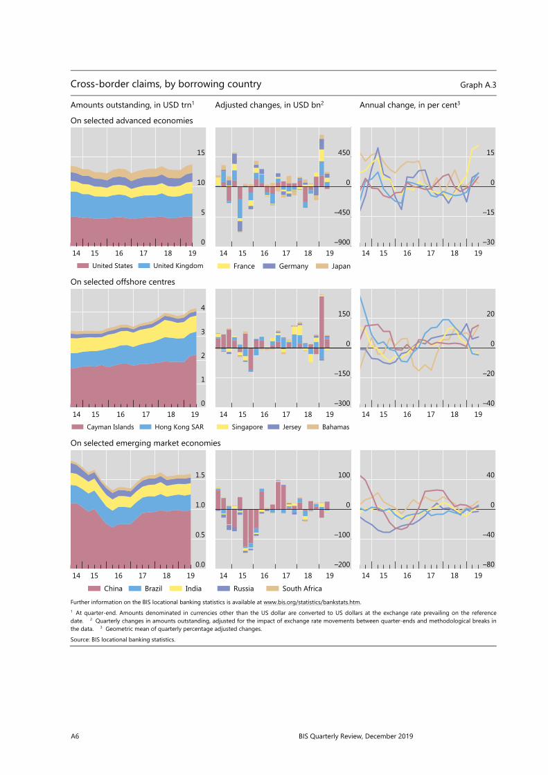
A6 BIS Quarterly Review, December 2019
Cross-border claims, by borrowing country Graph A.3
Amounts outstanding, in USD trn1 Adjusted changes, in USD bn2 Annual change, in per cent3 On selected advanced economies
On selected offshore centres
On selected emerging market economies
Further information on the BIS locational banking statistics is available at www.bis.org/statistics/bankstats.htm. 1 At quarter-end. Amounts denominated in currencies other than the US dollar are converted to US dollars at the exchange rate prevailing on the reference date. 2 Quarterly changes in amounts outstanding, adjusted for the impact of exchange rate movements between quarter-ends and methodological breaks in the data. 3 Geometric mean of quarterly percentage adjusted changes. Source: BIS locational banking statistics.
15
10
5
0191817161514
United States United Kingdom
450
0
–450
–900191817161514
France Germany Japan
15
0
–15
–30191817161514
4
3
2
1
0191817161514
Cayman Islands Hong Kong SAR
150
0
–150
–300191817161514
Singapore Jersey Bahamas
20
0
–20
–40191817161514
1.5
1.0
0.5
0.0191817161514
China Brazil India
100
0
–100
–200191817161514
Russia South Africa
40
0
–40
–80191817161514

BIS Quarterly Review, December 2019 A7
Cross-border claims, by nationality of reporting bank and currency of denomination Graph A.4
Amounts outstanding, in USD trn1 Adjusted changes, in USD bn2 Annual change, in per cent3 All currencies
US dollar
Euro
Further information on the BIS locational banking statistics is available at www.bis.org/statistics/bankstats.htm. 1 At quarter-end. Amounts denominated in currencies other than the US dollar are converted to US dollars at the exchange rate prevailing on the reference date. 2 Quarterly changes in amounts outstanding, adjusted for the impact of exchange rate movements between quarter-ends and methodological breaks in the data. 3 Geometric mean of quarterly percentage adjusted changes. Source: BIS locational banking statistics.
30
20
10
0191817161514
JapanUnited States
750
0
–750
–1,500191817161514
FranceGermany
Other
10
0
–10
–20191817161514
15
10
5
0191817161514
JapanUnited States
500
0
–500
–1,000191817161514
United KingdomSwitzerland
Other
15
0
–15
–30191817161514
9
6
3
0191817161514
GermanyFrance
400
0
–400
–800191817161514
NetherlandsUnited Kingdom
Other
20
0
–20
–40191817161514

A8 BIS Quarterly Review, December 2019
Cross-border liabilities of reporting banks Graph A.5
Amounts outstanding, in USD trn1 Adjusted changes, in USD bn2 Annual change, in per cent3 To emerging market economies
To central banks
By currency type and location
Further information on the BIS locational banking statistics is available at www.bis.org/statistics/bankstats.htm. 1 At quarter-end. Amounts denominated in currencies other than the US dollar are converted to US dollars at the exchange rate prevailing on the referencedate. 2 Quarterly changes in amounts outstanding, adjusted for the impact of exchange rate movements between quarter-ends and methodological breaks in the data. 3 Geometric mean of quarterly percentage adjusted changes. Source: BIS locational banking statistics.
3
2
1
0191817161514
Emerging Asia and PacificEmerging Europe
100
0
–100
–200191817161514
Emerging Latin America and CaribbeanEmerging Africa and Middle East
15
0
–15
–30191817161514
1.2
0.8
0.4
0.0191817161514
US dollar Euro Yen
50
0
–50
–100191817161514
Other currencies Unallocated
50
0
–50
–100191817161514
30
20
10
0191817161514
Cross-border in all currenciesResident in foreign currencies
600
0
–600
–1,200191817161514
Unallocated
5
0
–5
–10191817161514

BIS Quarterly Review, December 2019 A9
B Consolidated banking statistics
Consolidated claims of reporting banks on advanced economies Graph B.1
Foreign claims and local positions, in USD bn1, 2
Foreign claims of selected creditors, in USD bn1, 3
International claims, by sector and maturity, in per cent4
On the euro area
On the United States
On Japan
Further information on the BIS consolidated banking statistics is available at www.bis.org/statistics/bankstats.htm. 1 Amounts outstanding at quarter-end. Amounts denominated in currencies other than the US dollar are converted to US dollars at the exchange rate prevailingon the reference date. 2 Excludes domestic claims, ie claims on residents of a bank’s home country. 3 Foreign claims on a guarantor basis, by nationality of reporting bank. The banking systems shown are not necessarily the largest foreign bank creditors on each reference date. 4 As a percentage of international claims outstanding. 5 On an immediate counterparty basis. Includes the unconsolidated claims of banks headquartered outside but located inside CBS-reporting countries. 6 On a guarantor basis. Source: BIS consolidated banking statistics (CBS).
7,500
5,000
2,500
0191817161514
Foreign claims (immediate)5
Foreign claims (guarantor)6
Local claims in local currencyLocal liabilities in local currency
1,200
800
400
0191817161514
FRUS
GBJP
ES
45
30
15
0191817161514
BanksOfficial sectorNon-bank private sectorUp to and including 1 year
6,000
4,000
2,000
0191817161514
1,500
1,000
500
0191817161514
JPGB
CHFR
DE
60
40
20
0191817161514
900
600
300
0
1918171615
450
300
150
0
191817161514
USFR
GBTW
AU
50
25
0
191817161514

A10 BIS Quarterly Review, December 2019
Consolidated claims of reporting banks on emerging market economies Graph B.2
Foreign claims and local positions, in USD bn1, 2
Foreign claims of selected creditors, in USD bn1, 3
International claims, by sector and maturity, in per cent4
On China
On Turkey
On Brazil
Further information on the BIS consolidated banking statistics is available at www.bis.org/statistics/bankstats.htm. 1 Amounts outstanding at quarter-end. Amounts denominated in currencies other than the US dollar are converted to US dollars at the exchange rate prevailingon the reference date. 2 Excludes domestic claims, ie claims on residents of a bank’s home country. 3 Foreign claims on a guarantor basis, by nationality of reporting bank. The banking systems shown are not necessarily the largest foreign bank creditors on each reference date. 4 As a percentage of international claims. 5 On an immediate counterparty basis. Includes the unconsolidated claims of banks headquartered outside but located inside CBS-reporting countries. 6 On a guarantor basis . Source: BIS consolidated banking statistics (CBS).
1,200
800
400
0
191817161514
Foreign claims (immediate)5
Foreign claims (guarantor)6
Local claims in local currencyLocal liabilities in local currency
180
120
60
0
191817161514
GBUS
JPTW
FR
75
50
25
0
191817161514
BanksOfficial sectorNon-bank private sectorUp to and including 1 year
300
200
100
0
191817161514
75
50
25
0
191817161514
ESFR
GBUS
DE
60
40
20
0
191817161514
450
300
150
0
191817161514
180
120
60
0
191817161514
ESUS
GBJP
FR
60
40
20
0
191817161514

BIS Quarterly Review, December 2019 A11
C Debt securities statistics
Global debt securities markets1 Amounts outstanding, in trillions of US dollars2 Graph C.1
By market of issue By sector of issuer By currency of denomination3
DDS = domestic debt securities; IDS = international debt securities; TDS = total debt securities. FC = financial corporations; GG = general government; HH = households and non-profit institutions serving households; IO = international organisations; NFC = non-financial corporations. Further information on the BIS debt securities statistics is available at www.bis.org/statistics/secstats.htm. 1 Sample of countries varies across breakdowns shown. For countries that do not report TDS, data are estimated by the BIS as DDS plus IDS. For countries that donot report either TDS or DDS, data are estimated by the BIS as IDS. 2 At quarter-end. Amounts denominated in currencies other than the US dollar are converted to US dollars at the exchange rate prevailing on the reference date. 3 Where a currency breakdown is not available, DDS are assumed to be denominated in thelocal currency. Sources: Dealogic; Euroclear; Refinitiv; Xtrakter Ltd; national data; BIS debt securities statistics; BIS calculations.
Total debt securities, by residence and sector of issuer1 Amounts outstanding for the latest available data, in trillions of US dollars2 Graph C.2
Further information on the BIS debt securities statistics is available at www.bis.org/statistics/secstats.htm. 1 For countries that do not report TDS, data are estimated by the BIS as DDS plus IDS. 2 Amounts denominated in currencies other than the US dollar are converted to US dollars at the exchange rate prevailing on the reference date. Sources: National data; BIS debt securities statistics.
90
60
30
0
191817161514
TDSIDS
DDS
45
30
15
0
191817161514
GGFC
NFCIO
45
30
15
0
1918171615
USDEUR
JPYOTH
40
30
20
10
0
4
3
2
1
0IEKYKRAUESNLITCADEFRGBJPCNUS
Lhs Rhs
General governmentFinancial corporations
Non-financial corporationsHouseholds and non-profit institutions serving households

A12 BIS Quarterly Review, December 2019
Net issuance of international debt securities By issuer sector and currency of denomination, in billions of US dollars Graph C.3
US dollars Euro Pound Sterling
Further information is available at www.bis.org/statistics/secstats.htm.
Sources: Dealogic; Euroclear; Refinitiv; Xtrakter Ltd; BIS debt securities statistics.
International debt securities issued by financial and non-financial corporations1 Net issuance by region, in billions of US dollars2 Graph C.4
Developed countries Developing countries Offshore centres
Further information is available at www.bis.org/statistics/secstats.htm. 1 Excluding general government. 2 For a list of countries in each region, see Table C1 (http://stats.bis.org/statx/srs/table/c1). Sources: Dealogic; Euroclear; Refinitiv; Xtrakter Ltd; BIS debt securities statistics.
225
150
75
0
–75201920182017201620152014
BanksOther financial institutions
75
0
–75
–150201920182017201620152014
Non-financial corporations
40
20
0
–20
–40201920182017201620152014
General governmentInternational organizations
200
150
100
50
0
–50
–100201920182017201620152014
60
30
0
–30
–60201920182017201620152014
Nationals Residents
120
90
60
30
0
–30201920182017201620152014
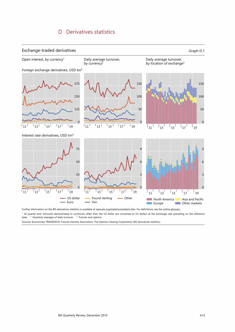
BIS Quarterly Review, December 2019 A13
D Derivatives statistics
Exchange-traded derivatives Graph D.1
Open interest, by currency1 Daily average turnover, by currency2
Daily average turnover, by location of exchange2
Foreign exchange derivatives, USD bn3
Interest rate derivatives, USD trn3
Further information on the BIS derivatives statistics is available at www.bis.org/statistics/extderiv.htm. For definitions, see the online glossary. 1 At quarter-end. Amounts denominated in currencies other than the US dollar are converted to US dollars at the exchange rate prevailing on the referencedate. 2 Quarterly averages of daily turnover. 3 Futures and options. Sources: Euromoney TRADEDATA; Futures Industry Association; The Options Clearing Corporation; BIS derivatives statistics.
375
250
125
01917151311
150
100
50
01917151311
150
100
50
0
1917151311
75
50
25
01917151311
US dollarEuro
9
6
3
01917151311
Pound sterlingYen
Other
9
6
3
0
1917151311
North AmericaEurope
Asia and PacificOther markets

A14 BIS Quarterly Review, December 2019
Global OTC derivatives markets1 Graph D.2
Notional principal Gross market value Gross credit exposure USD trn USD trn Per cent USD trn
Further information on the BIS derivatives statistics is available at www.bis.org/statistics/derstats.htm. For definitions, see the online glossary. 1 At half-year end (end-June and end-December). Amounts denominated in currencies other than the US dollar are converted to US dollars at the exchange rateprevailing on the reference date. Source: BIS derivatives statistics.
OTC foreign exchange derivatives Notional principal1 Graph D.3
By currency By maturity By sector of counterparty USD trn Per cent Per cent USD trn
Further information on the BIS derivatives statistics is available at www.bis.org/statistics/derstats.htm. For definitions, see the online glossary. 1 At half-year end (end-June and end-December). Amounts denominated in currencies other than the US dollar are converted to US dollars at the exchange rateprevailing on the reference date. Source: BIS derivatives statistics.
600
400
200
01917151311
Interest rateFXEquity
30
20
10
01917151311
CommoditiesCDS
30
20
10
0
4.5
3.0
1.5
0.01917151311
Share of gross market value (lhs)Amounts (rhs)
80
60
40
20
019171513
US dollarEuro
Pound sterlingYen
100
75
50
25
01917151311
≤ 1 year> 1 year & ≤ 5 years> 5 years
8
6
4
2
0
80
60
40
20
01917151311
Rhs:Share of CCPs (lhs)
Reporting dealersOther financial institutionsNon-financial institutions

BIS Quarterly Review, December 2019 A15
OTC interest rate derivatives Notional principal1 Graph D.4
By currency By maturity By sector of counterparty USD trn Per cent Per cent USD trn
Further information on the BIS derivatives statistics is available at www.bis.org/statistics/derstats.htm. For definitions, see the online glossary. 1 At half-year end (end-June and end-December). Amounts denominated in currencies other than the US dollar are converted to US dollars at the exchange rateprevailing on the reference date. Source: BIS derivatives statistics.
OTC equity-linked derivatives Notional principal1 Graph D.5
By equity market By maturity By sector of counterparty USD trn Per cent Per cent USD trn
Further information on the BIS derivatives statistics is available at www.bis.org/statistics/derstats.htm. For definitions, see the online glossary. 1 At half-year end (end-June and end-December). Amounts denominated in currencies other than the US dollar are converted to US dollars at the exchange rate prevailing on the reference date. Source: BIS derivatives statistics.
240
180
120
60
019171513
US dollarEuro
Pound sterlingYen
100
75
50
25
01917151311
≤ 1 year> 1 year & ≤ 5 years> 5 years
82
80
78
76
74
600
450
300
150
01917151311
Rhs:Share of CCPs (lhs)
Reporting dealersOther financial institutionsNon-financial institutions
4
3
2
1
019171513
United StatesEuropean countries
JapanOther
100
75
50
25
01917151311
≤ 1 year> 1 year & ≤ 5 years> 5 years
8
6
4
2
0
8
6
4
2
01917151311
Rhs:Share of CCPs (lhs)
Reporting dealersOther financial institutionsNon-financial institutions

A16 BIS Quarterly Review, December 2019
OTC commodity derivatives1 Graph D.6
Notional principal, by instrument Notional principal, by commodity Gross market value, by commodity Per cent USD trn USD trn
Further information on the BIS derivatives statistics is available at www.bis.org/statistics/derstats.htm. For definitions, see the online glossary. 1 At half-year end (end-June and end-December). Amounts denominated in currencies other than the US dollar are converted to US dollars at the exchange rateprevailing on the reference date. Source: BIS derivatives statistics.
Credit default swaps1 Graph D.7
Notional principal Notional principal with central counterparties (CCPs)
Impact of netting
Per cent USD trn Per cent USD trn Per cent USD trn
Further information on the BIS derivatives statistics is available at www.bis.org/statistics/derstats.htm. For definitions, see the online glossary. 1 At half-year end (end-June and end-December). Amounts denominated in currencies other than the US dollar are converted to US dollars at the exchange rateprevailing on the reference date. Source: BIS derivatives statistics.
100
75
50
25
01917151311
Forwards and swaps Options
4
3
2
1
01917151311
Other commodities Gold
0.8
0.6
0.4
0.2
0.01917151311
Other precious metals
20
15
10
5
0
40
30
20
10
0191715
Rhs:Gross market value/notional (lhs)
Single-name notionalMulti-name notional
60
45
30
15
0
6.0
4.5
3.0
1.5
0.0191817161514
Rhs:CCPs/total (lhs)
Single-name notionalMulti-name notional
30
25
20
15
10
1.2
0.9
0.6
0.3
0.0191817161514
Rhs:Net/gross market values (lhs)
Gross market valuesNet market values

BIS Quarterly Review, December 2019 A17
Growth of central clearing Notional amounts outstanding by counterparty, in per cent Graph D.9
Interest rate derivatives Credit default swaps
Further information on the BIS derivatives statistics is available at www.bis.org/statistics/derstats.htm. For definitions, see the online glossary. 1 As a percentage of notional amounts outstanding against all counterparties. 2 Including central counterparties but excluding reporting dealers. 3 For interest rate derivatives, data for CCPs prior to end-June 2016 are estimated by indexing the amounts reported at end-June 2016 to the growth since 2008 of notionalamounts outstanding cleared through LCH’s SwapClear service. 4 Proportion of trades that are cleared, estimated as (CCP / 2) / (1 – (CCP / 2)), where CCP represents the share of notional amounts outstanding that dealers report against CCPs. CCPs’ share is halved to adjust for the potential double-counting of inter-dealer trades novated to CCPs. Sources: LCH.Clearnet Group Ltd; BIS OTC derivatives statistics (Table D7 and Table D10.1); BIS calculations.
80
60
40
20
019171513110907
Reporting dealers1
Other financial institutions1, 2
80
60
40
20
019171513110907
Central counterparties1, 3
Estimated minimum clearing rate4
Concentration in global OTC derivatives markets Herfindahl index1 Graph D.8
Foreign exchange derivatives2 Interest rate swaps Equity-linked options
Further information on the BIS derivatives statistics is available at www.bis.org/statistics/derstats.htm. For definitions, see the online glossary. 1 The index ranges from 0 to 10,000, where a lower number indicates that there are many dealers with similar market shares (as measured by notional principal) and a higher number indicates that the market is dominated by a few reporting dealers. 2 Foreign exchange forwards, foreign exchange swaps and currencyswaps. Source: BIS derivatives statistics.
1,000
800
600
40019171513
USDEUR
GBPJPY
1,400
1,000
600
20019171513
CHFCAD
SEK
6,400
4,400
2,400
40019171513
United StatesJapanEurope
Latin AmericaOther Asia

A18 BIS Quarterly Review, December 2019
E Global liquidity indicators
US dollar credit outside the United States1
Annual change, in per cent Graph E.1
Further information on the BIS global liquidity indicators is available at www.bis.org/statistics/gli.htm. 1 Annual growth of US dollar-denominated credit to non-banks outside the United States. 2 Annual growth of the US dollar nominal effective exchange rate. Sources: Datastream; Dealogic; Euroclear; Refinitiv; Xtrakter Ltd; national data; BIS locational banking statistics; BIS effective exchange rate statistics; BIS calculations.
20
10
0
–10
–202019201720152013201120092007200520032001
Total credit Loans Debt securities NEER2

BIS Quarterly Review, December 2019 A19
Global bank credit to the private non-financial sector, by residence of borrower Banks’ cross-border credit plus local credit in all currencies1 Graph E.2
All countries2 United States Euro area3
% of GDP Annual change, % % of GDP Annual change, % % of GDP Annual change, %
Emerging Asia4 Latin America5 Central Europe6
% of GDP Annual change, % % of GDP Annual change, % % of GDP Annual change, %
Further information on the BIS global liquidity indicators is available at www.bis.org/statistics/gli.htm. 1 Cross-border claims of LBS reporting banks to the non-bank sector plus local claims of all banks to the private non-financial sector. Weighted averages of the economies listed, based on four-quarter moving sums of GDP. 2 Australia, Canada, Denmark, Japan, New Zealand, Norway, Russia, Saudi Arabia, South Africa,Sweden, Switzerland, Turkey and the United Kingdom, plus the countries in the other panels. 3 Austria, Belgium, Finland, France, Germany, Greece, Ireland, Italy, the Netherlands, Portugal and Spain. 4 China, Hong Kong SAR, India, Indonesia, Korea, Malaysia, Singapore and Thailand. 5 Argentina, Brazil, Chile and Mexico. 6 The Czech Republic, Hungary and Poland. Sources: BIS credit to the non-financial sector; BIS locational banking statistics; BIS calculations.
120
90
60
30
0
24
12
0
–12
–2419161310070401
120
90
60
30
0
24
12
0
–12
–2419161310070401
120
90
60
30
0
24
12
0
–12
–2419161310070401
120
90
60
30
0
50
25
0
–25
–5019161310070401
120
90
60
30
0
50
25
0
–25
–5019161310070401
(rhs):Annual changes
(lhs):Amounts outstanding
Cross-border creditLocal credit
120
90
60
30
0
50
25
0
–25
–5019161310070401
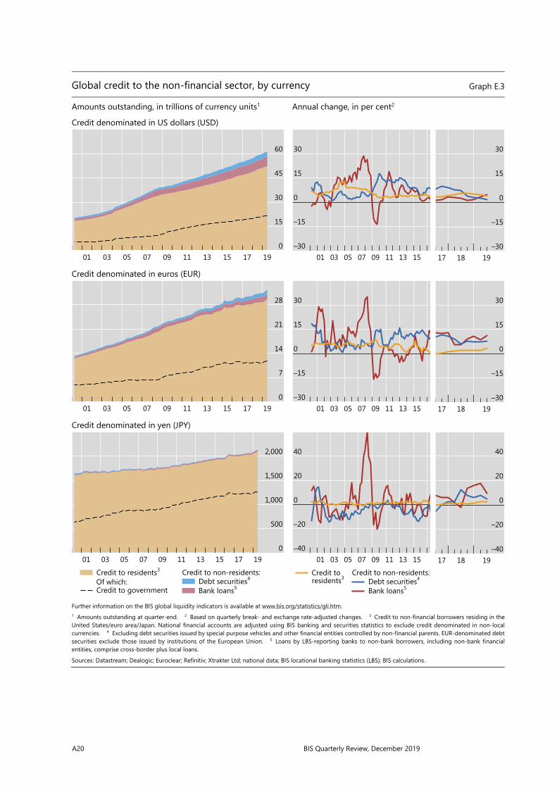
A20 BIS Quarterly Review, December 2019
Global credit to the non-financial sector, by currency Graph E.3
Amounts outstanding, in trillions of currency units1 Annual change, in per cent2
Credit denominated in US dollars (USD)
Credit denominated in euros (EUR)
Credit denominated in yen (JPY)
Further information on the BIS global liquidity indicators is available at www.bis.org/statistics/gli.htm. 1 Amounts outstanding at quarter-end. 2 Based on quarterly break- and exchange rate-adjusted changes. 3 Credit to non-financial borrowers residing in the United States/euro area/Japan. National financial accounts are adjusted using BIS banking and securities statistics to exclude credit denominated in non-local currencies. 4 Excluding debt securities issued by special purpose vehicles and other financial entities controlled by non-financial parents. EUR-denominated debt securities exclude those issued by institutions of the European Union. 5 Loans by LBS-reporting banks to non-bank borrowers, including non-bank financial entities, comprise cross-border plus local loans. Sources: Datastream; Dealogic; Euroclear; Refinitiv; Xtrakter Ltd; national data; BIS locational banking statistics (LBS); BIS calculations.
60
45
30
15
019171513110907050301
30
15
0
–15
–301513110907050301
30
15
0
–15
–30191817
28
21
14
7
019171513110907050301
30
15
0
–15
–301513110907050301
30
15
0
–15
–30191817
2,000
1,500
1,000
500
019171513110907050301
Of which:Credit to residents3
Debt securities4
Bank loans5
Credit to non-residents:
Credit to government
40
20
0
–20
–401513110907050301
Credit toresidents3 Debt securities4
Bank loans5
Credit to non-residents:
40
20
0
–20
–40191817

BIS Quarterly Review, December 2019 A21
Foreign currency credit to non-banks in EMDEs Graph E.5
US dollar-denominated credit by region Foreign currency credit to selected EMDEs1
USD trn USD bn
Further information on the BIS global liquidity indicators is available at www.bis.org/statistics/gli.htm. 1 Amounts outstanding for the latest available data. Sources: Datastream; Dealogic; Euroclear; Refinitiv; Xtrakter Ltd; national data; BIS locational banking statistics (LBS); BIS calculations.
3
2
1
019171513110907050301
Emerging EuropeLatin America and Caribbean
Africa and Middle EastEmerging Asia-Pacific
450
300
150
0MYZATWCLINKRARSABRRUIDTRMXCN
USDDenominated in: EUR JPY
US dollar-denominated credit to non-banks outside the United States1 Graph E.4
World EMDEs Per cent USD tn Per cent USD tn
Further information on the BIS global liquidity indicators is available at www.bis.org/statistics/gli.htm. 1 Non-banks comprise non-bank financial entities, non-financial corporations, governments, households and international organisations. 2 Loans by LBS-reporting banks to non-bank borrowers, including non-bank financial entities, comprise cross-border plus local loans. Sources: Datastream; Dealogic; Euroclear; Refinitiv; Xtrakter Ltd; national data; BIS locational banking statistics (LBS); BIS calculations.
58
54
50
46
12
8
4
019171513110907050301
Share of bank loansLhs:
65
60
55
50
3
2
1
019171513110907050301
Bonds issued by non-banksBank loans to non-banks2
Amounts outstanding (rhs):
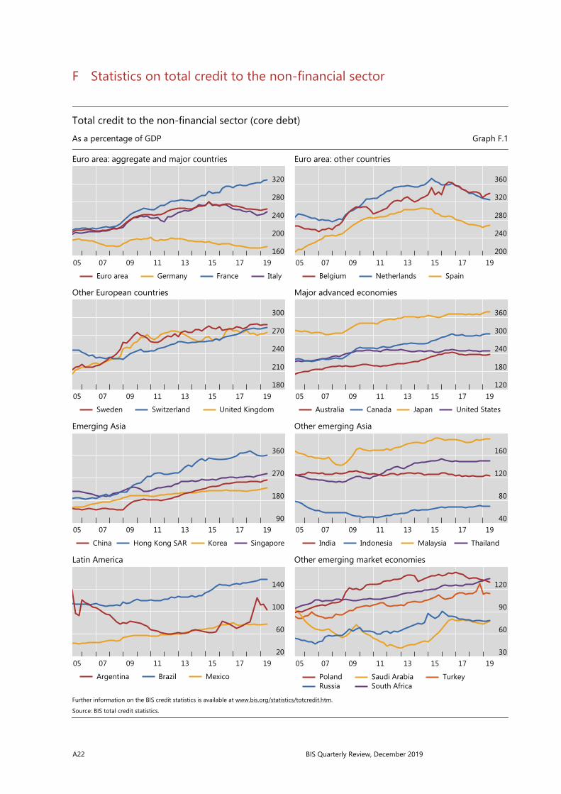
A22 BIS Quarterly Review, December 2019
F Statistics on total credit to the non-financial sector
Total credit to the non-financial sector (core debt) As a percentage of GDP Graph F.1
Euro area: aggregate and major countries Euro area: other countries
Other European countries Major advanced economies
Emerging Asia Other emerging Asia
Latin America Other emerging market economies
Further information on the BIS credit statistics is available at www.bis.org/statistics/totcredit.htm. Source: BIS total credit statistics.
320
280
240
200
1601917151311090705
Euro area Germany France Italy
360
320
280
240
2001917151311090705
Belgium Netherlands Spain
300
270
240
210
1801917151311090705
Sweden Switzerland United Kingdom
360
300
240
180
1201917151311090705
Australia Canada Japan United States
360
270
180
901917151311090705
China Hong Kong SAR Korea Singapore
160
120
80
401917151311090705
India Indonesia Malaysia Thailand
140
100
60
201917151311090705
Argentina Brazil Mexico
120
90
60
301917151311090705
PolandRussia
Saudi ArabiaSouth Africa
Turkey

BIS Quarterly Review, December 2019 A23
Total credit to the private non-financial sector (core debt) As a percentage of GDP Graph F.2
Euro area: aggregate and major countries Euro area: other countries
Other European countries Major advanced economies
Emerging Asia Other emerging Asia
Latin America Other emerging market economies
Further information on the BIS credit statistics is available at www.bis.org/statistics/totcredit.htm. Source: BIS total credit statistics.
200
160
120
801917151311090705
Euro area Germany France Italy
275
225
175
1251917151311090705
Belgium Netherlands Spain
240
210
180
1501917151311090705
Sweden Switzerland United Kingdom
210
180
150
1201917151311090705
Australia Canada Japan United States
280
210
140
701917151311090705
China Hong Kong SAR Korea Singapore
120
80
40
01917151311090705
India Indonesia Malaysia Thailand
60
40
20
01917151311090705
Argentina Brazil Mexico
80
60
40
201917151311090705
PolandRussia
Saudi ArabiaSouth Africa
Turkey

A24 BIS Quarterly Review, December 2019
Bank credit to the private non-financial sector (core debt) As a percentage of GDP Graph F.3
Euro area: aggregate and major countries Euro area: other countries
Other European countries Major advanced economies
Emerging Asia Other emerging Asia
Latin America Other emerging market economies
Further information on the BIS credit statistics is available at www.bis.org/statistics/totcredit.htm. Source: BIS total credit statistics.
100
90
80
70
601917151311090705
Euro area Germany France Italy
150
120
90
60
301917151311090705
Belgium Netherlands Spain
160
140
120
100
801917151311090705
Sweden Switzerland United Kingdom
120
90
60
30
01917151311090705
Australia Canada Japan United States
240
180
120
601917151311090705
China Hong Kong SAR Korea Singapore
120
80
40
01917151311090705
India Indonesia Malaysia Thailand
60
45
30
15
01917151311090705
Argentina Brazil Mexico
75
60
45
30
151917151311090705
PolandRussia
Saudi ArabiaSouth Africa
Turkey

BIS Quarterly Review, December 2019 A25
Total credit to households (core debt) As a percentage of GDP Graph F.4
Euro area: aggregate and major countries Euro area: other countries
Other European countries Major advanced economies
Emerging Asia Other emerging Asia
Latin America Other emerging market economies
Further information on the BIS credit statistics is available at www.bis.org/statistics/totcredit.htm. Source: BIS total credit statistics.
70
60
50
40
301917151311090705
Euro area Germany France Italy
120
100
80
60
401917151311090705
Belgium Netherlands Spain
120
100
80
60
401917151311090705
Sweden Switzerland United Kingdom
120
100
80
60
401917151311090705
Australia Canada Japan United States
80
60
40
20
01917151311090705
China Hong Kong SAR Korea Singapore
80
60
40
20
01917151311090705
India Indonesia Malaysia Thailand
28
21
14
7
01917151311090705
Argentina Brazil Mexico
40
30
20
10
01917151311090705
PolandRussia
Saudi ArabiaSouth Africa
Turkey
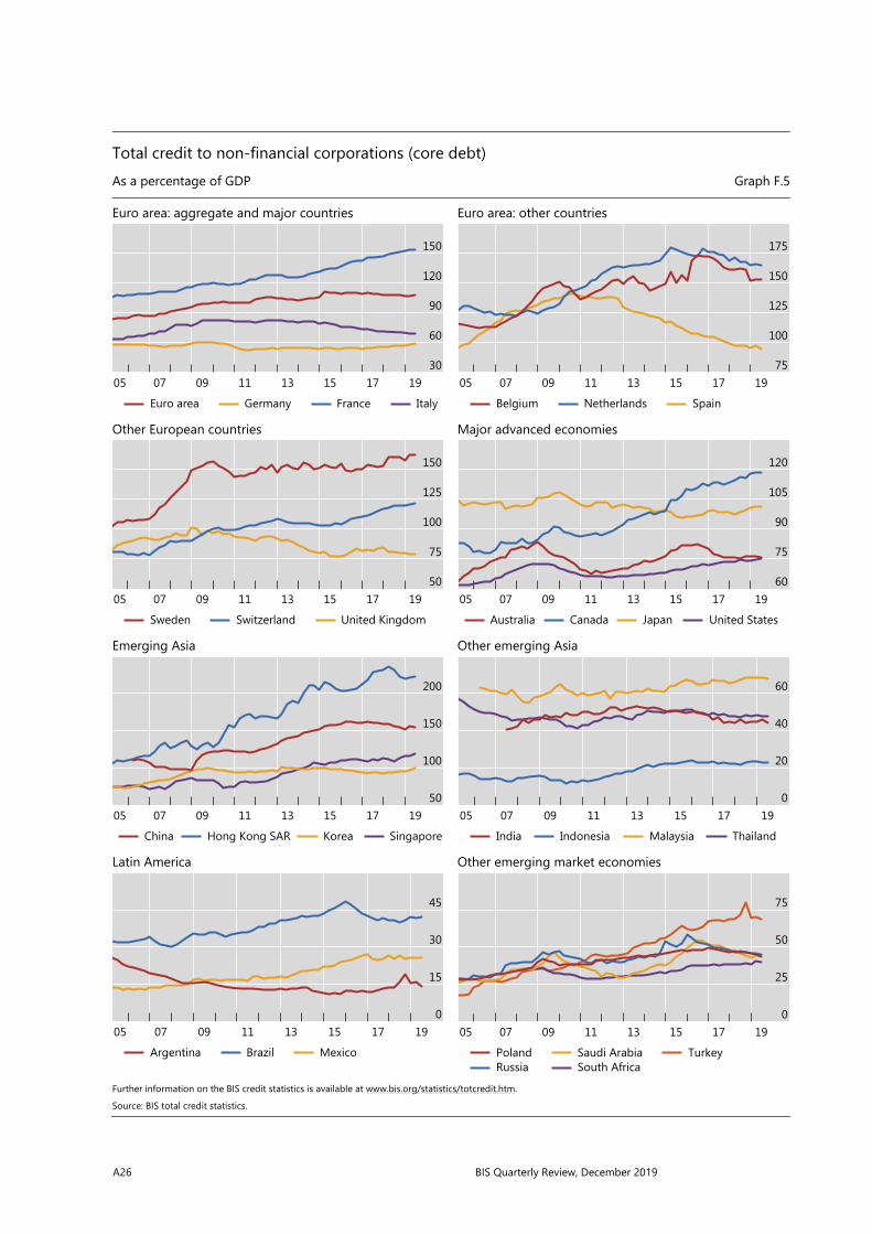
A26 BIS Quarterly Review, December 2019
Total credit to non-financial corporations (core debt) As a percentage of GDP Graph F.5
Euro area: aggregate and major countries Euro area: other countries
Other European countries Major advanced economies
Emerging Asia Other emerging Asia
Latin America Other emerging market economies
Further information on the BIS credit statistics is available at www.bis.org/statistics/totcredit.htm. Source: BIS total credit statistics.
150
120
90
60
301917151311090705
Euro area Germany France Italy
175
150
125
100
751917151311090705
Belgium Netherlands Spain
150
125
100
75
501917151311090705
Sweden Switzerland United Kingdom
120
105
90
75
601917151311090705
Australia Canada Japan United States
200
150
100
501917151311090705
China Hong Kong SAR Korea Singapore
60
40
20
01917151311090705
India Indonesia Malaysia Thailand
45
30
15
01917151311090705
Argentina Brazil Mexico
75
50
25
01917151311090705
PolandRussia
Saudi ArabiaSouth Africa
Turkey

BIS Quarterly Review, December 2019 A27
Total credit to the government sector at market value (core debt)1 As a percentage of GDP Graph F.6
Euro area: aggregate and major countries Euro area: other countries
Other European countries Major advanced economies
Emerging Asia Other emerging market economies
Further information on the BIS credit statistics is available at www.bis.org/statistics/totcredit.htm. 1 Consolidated data for the general government sector. Source: BIS total credit statistics.
150
125
100
75
501917151311090705
Euro area Germany France Italy
125
100
75
50
251917151311090705
Belgium Netherlands Spain
100
80
60
40
20
1917151311090705
Sweden Switzerland United Kingdom
200
150
100
50
0
1917151311090705
Australia Canada Japan United States
55
45
35
25
151917151311090705
Korea
55
45
35
25
151917151311090705
Poland Turkey

A28 BIS Quarterly Review, December 2019
Total credit to the government sector at nominal value (core debt)1 As a percentage of GDP Graph F.7
Euro area: aggregate and major countries Euro area: other countries
Other European countries Major advanced economies
Emerging Asia Other emerging Asia
Latin America Other emerging market economies
Further information on the BIS credit statistics is available at www.bis.org/statistics/totcredit.htm. 1 Consolidated data for the general government sector; central government for Argentina, Indonesia, Malaysia, Mexico, Saudi Arabia and Thailand. Source: BIS total credit statistics.
125
100
75
501917151311090705
Euro area Germany France Italy
100
75
50
251917151311090705
Belgium Netherlands Spain
90
75
60
45
30
1917151311090705
Sweden Switzerland United Kingdom
200
150
100
50
0
1917151311090705
Australia Canada Japan United States
100
75
50
25
0
1917151311090705
China Hong Kong SAR Singapore
75
60
45
30
15
1917151311090705
India Indonesia Malaysia Thailand
100
75
50
25
0
1917151311090705
Argentina Brazil Mexico
80
60
40
20
0
1917151311090705
PolandRussia
Saudi ArabiaSouth Africa
Turkey
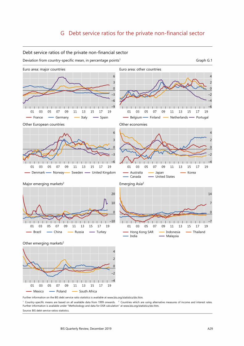
BIS Quarterly Review, December 2019 A29
G Debt service ratios for the private non-financial sector
Debt service ratios of the private non-financial sector Deviation from country-specific mean, in percentage points1 Graph G.1
Euro area: major countries Euro area: other countries
Other European countries Other economies
Major emerging markets2 Emerging Asia2
Other emerging markets2
Further information on the BIS debt service ratio statistics is available at www.bis.org/statistics/dsr.htm. 1 Country-specific means are based on all available data from 1999 onwards. 2 Countries which are using alternative measures of income and interest rates.Further information is available under “Metholodogy and data for DSR calculation” at www.bis.org/statistics/dsr.htm. Source: BIS debt service ratios statistics.
6
3
0
–3
–6
–919171513110907050301
France Germany Italy Spain
4
2
0
–2
–4
–619171513110907050301
Belgium Finland Netherlands Portugal
6
3
0
–3
–619171513110907050301
Denmark Norway Sweden United Kingdom
4
2
0
–2
–419171513110907050301
AustraliaCanada
JapanUnited States
Korea
20
10
0
–1019171513110907050301
Brazil China Russia Turkey
14
7
0
–719171513110907050301
Hong Kong SARIndia
IndonesiaMalaysia
Thailand
4
2
0
–2
–419171513110907050301
Mexico Poland South Africa

A30 BIS Quarterly Review, December 2019
Debt service ratios of households Deviation from country-specific mean, in percentage points1 Graph G.2
Euro area: major countries Euro area: other countries
Other European countries Other economies
Further information on the BIS debt service ratio statistics is available at www.bis.org/statistics/dsr.htm. 1 Country-specific means are based on all available data from 1999 onwards. Source: BIS debt service ratios statistics.
4
2
0
–2
–419171513110907050301
France Germany Italy Spain
4
2
0
–2
–419171513110907050301
Belgium Finland Netherlands Portugal
4
2
0
–2
–419171513110907050301
Denmark Norway Sweden United Kingdom
2
0
–2
–4
–619171513110907050301
AustraliaCanada
JapanUnited States
Korea

BIS Quarterly Review, December 2019 A31
Debt service ratios of non-financial corporations Deviation from country-specific mean, in percentage points1 Graph G.3
Euro area: major countries Euro area: other countries
Other European countries Other economies
Further information on the BIS debt service ratio statistics is available at www.bis.org/statistics/dsr.htm. 1 Country-specific means are based on all available data from 1999 onwards. Source: BIS debt service ratios statistics.
20
10
0
–10
–2019171513110907050301
France Germany Italy Spain
20
10
0
–10
–2019171513110907050301
Belgium Finland Netherlands Portugal
20
10
0
–10
–2019171513110907050301
Denmark Norway Sweden United Kingdom
20
10
0
–10
–2019171513110907050301
AustraliaCanada
JapanUnited States
Korea

A32 BIS Quarterly Review, December 2019
H Property price statistics
Real residential property prices CPI-deflated, 2010 = 100 Graph H.1
Euro area: aggregate and major countries Euro area: other countries
Other European countries Major advanced economies
Emerging Asia Other emerging Asia
Latin America Other emerging market economies
Further information on the BIS property price statistics is available at www.bis.org/statistics/pp.htm. Source: BIS property prices statistics.
120
100
80
601917151311090705
Euro area Germany France Italy
120
100
80
601917151311090705
Belgium Netherlands Spain
140
120
100
80
601917151311090705
Sweden Switzerland United Kingdom
140
120
100
80
601917151311090705
Australia Canada Japan United States
180
140
100
60
201917151311090705
China Hong Kong SAR Korea Singapore
160
140
120
100
801917151311090705
India Indonesia Malaysia Thailand
125
100
75
50
251917151311090705
Brazil Mexico
125
100
75
50
251917151311090705
Poland Russia South Africa Turkey

BIS Quarterly Review, December 2019 A33
I Effective and US dollar exchange rate statistics
Real effective exchange rates CPI-based, 1995–2005 = 1001 Graph I.1
Euro area: aggregate and major countries Euro area: other countries
Other European countries Major advanced economies
Emerging Asia Other emerging Asia
Latin America Other emerging market economies
Further information on the BIS effective exchange rate statistics is available at www.bis.org/statistics/eer.htm. 1 An increase indicates a real-term appreciation of the local currency against a broad basket of currencies. Source: BIS effective exchange rates statistics.
120
110
100
90
801917151311090705
Euro area Germany France Italy
120
110
100
90
801917151311090705
Belgium Netherlands Spain
120
100
80
601917151311090705
Sweden United Kingdom Switzerland
125
100
75
501917151311090705
Australia Canada Japan United States
125
100
75
501917151311090705
China Hong Kong SAR Korea Singapore
120
100
80
601917151311090705
India Indonesia Malaysia Thailand
130
100
70
40
101917151311090705
Argentina Brazil Mexico
150
125
100
75
501917151311090705
PolandRussia
Saudi ArabiaSouth Africa
Turkey

A34 BIS Quarterly Review, December 2019
US dollar exchange rates Indices, 1995–2005 = 1001 Graph I.2
Major advanced economies Other advanced economies
Emerging Asia Other emerging Asia
Latin America Other emerging market economies
Further information on the exchange rate statistics is available at www.bis.org/statistics/xrusd.htm. 1 An increase indicates an appreciation of the local currency against the US dollar. Source: BIS US dollar exchange rates statistics.
140
120
100
80
601917151311090705
Euro area Japan United Kingdom
160
140
120
100
801917151311090705
Australia Canada Sweden Switzerland
140
120
100
80
601917151311090705
China Hong Kong SAR Korea Singapore
125
100
75
50
251917151311090705
India Indonesia Malaysia Thailand
100
75
50
25
01917151311090705
Argentina Brazil Mexico
140
100
60
20
1917151311090705
PolandRussia
Saudi ArabiaSouth Africa
Turkey

BIS Quarterly Review, December 2019 A35
J Credit-to-GDP gaps
Credit-to-GDP gaps In percentage points of GDP Graph J.1
Euro area: aggregate and major countries Euro area: other countries
Other European countries Major advanced economies
Emerging Asia Other emerging Asia
Latin America Other emerging market economies
1 Estimates based on series on total credit to the private non-financial sector. The credit-to-GDP gap is defined as the difference between the credit-to-GDP ratio and its long-term trend; the long-term trend is calculated using a one-sided Hodrick-Prescott filter with a smoothing parameter of 400,000. Further information on the BIS credit-to-GDP gaps is available at www.bis.org/statistics/c_gaps.htm. Source: BIS credit-to-GDP gaps statistics.
10
0
–10
–20
–301917151311090705
Euro area Germany France Italy
25
0
–25
–50
–751917151311090705
Belgium Netherlands Spain
20
0
–20
–401917151311090705
Sweden Switzerland United Kingdom
10
0
–10
–20
–301917151311090705
Australia Canada Japan United States
40
20
0
–20
–401917151311090705
China Hong Kong SAR Korea Singapore
20
0
–20
–40
–601917151311090705
India Indonesia Malaysia Thailand
10
0
–10
–201917151311090705
Argentina Brazil Mexico
10
0
–10
–201917151311090705
PolandRussia
Saudi ArabiaSouth Africa
Turkey

A36 BIS Quarterly Review, December 2019
K Consumer prices
Consumer prices Year-on-year percentage changes Graph K.1
Euro area: aggregate and major countries Euro area: other countries
Other European countries Major advanced economies
Emerging Asia Other emerging Asia
Latin America Other emerging market economies
Further information on the BIS consumer prices is available at www.bis.org/statistics/cp.htm. Source: BIS consumer price statistics.
4
2
0
–21917151311090705
Euro area Germany France Italy
4
2
0
–21917151311090705
Belgium Netherlands Spain
4
2
0
–2
–41917151311090705
Sweden Switzerland United Kingdom
4
2
0
–2
–41917151311090705
Australia Canada Japan United States
9
6
3
0
–31917151311090705
China Hong Kong SAR Korea Singapore
15
10
5
0
–51917151311090705
India Indonesia Malaysia Thailand
40
20
0
1917151311090705
Argentina Brazil Mexico
20
10
0
1917151311090705
PolandRussia
Saudi ArabiaSouth Africa
Turkey

BIS Quarterly Review, December 2019 A37
L Central bank policy rates
Central bank policy or representative rates Month-end; in per cent Graph L.1
Major advanced economies Other advanced economies
Emerging Asia Other emerging Asia
Latin America Other emerging market economies
Further information on the policy rates is available at www.bis.org/statistics/cbpol.htm. Source: BIS policy rates statistics.
6
4
2
0
–21917151311090705
Euro areaJapan
United KingdomUnited States
6
4
2
0
–21917151311090705
Australia Canada Sweden Switzerland
6
4
2
0
–21917151311090705
China Hong Kong SAR Korea
12
9
6
3
01917151311090705
India Indonesia Malaysia Thailand
80
60
40
20
01917151311090705
Argentina Brazil Mexico
20
15
10
5
01917151311090705
PolandRussia
Saudi ArabiaSouth Africa
Turkey


