58
Bivariate Statistics (continued) & Multivariate Statistics) Chapter 11
| Date post: | 31-Dec-2015 |
| Category: |
Documents |
| Upload: | caldwell-porter |
| View: | 60 times |
| Download: | 6 times |

Bivariate Statistics (continued) & Multivariate Statistics)
Chapter 11

Today’s Topics
• Bivariate Statistics (Measures of Association)• Trivariate Statistics (control variables, partials)• Constructing tables & interpreting descriptive
statistics• Different Styles of Presentation• Preparation for Lab activities and work on
Final Assignment

Recall (Lecture 2) *Types of variables*
• independent variable (cause)• dependent variable (effect)• intervening variable – (occurs between the independent and the
dependent variable temporally)
• control variable – (temporal occurance varies, illustrations later
today)

Causal Relationships
• proposed for testing (NOT like assumptions)• 5 characteristics of causal hypothesis (p.128)
– at least 2 variables– cause-effect relationship (cause must come before
effect)– can be expressed as prediction– logically linked to research question+ a theory– falsifiable

Types of Correlations & Causal Relationships between Two Variables
X=independent variable Y=dependent variable
• Positive Correlation (Direct relationship)– when X increases Y increases or vice versa
• Negative Correlation (Indirect or inverse relationship)– when X increases Y decreases or vice versa
• Independence – no relationship (null hypothesis)
• Co-variation – vary together ( a type of association but not necessarily causal)
YX-
YX+

Interpreting a Relationship between two variables
• Do the patterns in the tables mean that there is a relationship between the two variables?
• If there is a relationship, how strong is it? Are the results statistically significant? Are the results meaningful ?
• Methods for studying relationships– Create Cross-tabulations & percentaged tables– Create Graphs, charts (like scattergrams or plots)– Use a set of statistics called measures of association

Using Graphs to show relations (royal wedding and electricity use)

Five Common Measures of Association between Two Variables

General Idea of Statistical Significance
• In general English ‘significance’ means important or meaningful but this is NOT how the term is used in statistics
• Tests of statistical significance show you how likely a result is due to chance.

Interpreting Statistical Significance Levels
• “The most common level, used to mean something is good enough to be believed, is .95. This means that the finding has a 95% chance of being true. However, this value is also used in a misleading way.
• No statistical package will show you "95%" or ".95" to indicate this level.
• Instead it will show you ".05," meaning that the finding has a five percent (.05) chance of not being true, which is the converse of a 95% chance of being true.
• To find the significance level, subtract the number shown from one. For example, a value of ".01" means that there is a 99% (1-.01=.99) chance of it being true.”
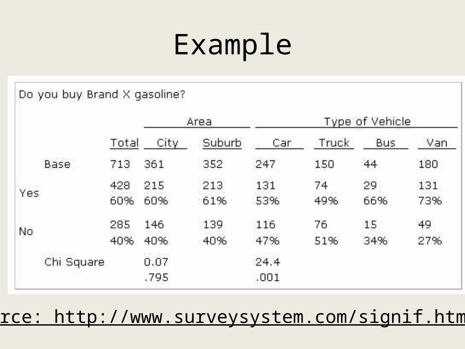
Example
Source: http://www.surveysystem.com/signif.htm
Discussion of Example• “Refer to the preceeding table. The chi
(pronounced kie like pie) squares at the bottom of the table show two rows of numbers.
• The top row numbers of 0.07 and 24.4 are the chi square statistics themselves. The meaning of these statistics may be ignored for the purposes of this article. The second row contains values .795 and .001. These are the significance levels.”
Discussion• “In this table, there is probably no difference in
purchases of gasoline X by people in the city center and the suburbs, because the probability is .795 (i.e., there is only a 20.5% chance that the difference is true).
• In contrast the high significance level for type of vehicle (.001 or 99.9%) indicates there is almost certainly a true difference in purchases of Brand X by owners of different vehicles in the population from which the sample was drawn. “

Correlation Coefficient
• statistics which can help to describe data sets which contain variables measured at the interval and ratio levels.
• measures of association between two (or more) variables. • tests whether a relationship exists between two variables. • indicates both the strength of the association and its
direction (direct or inverse). • Pearson product-moment correlation coefficient, written as r,
can describe a linear relationship between two variables.

Correlation Coefficient • Is there a relationship between:
• the budget of the police department and the crime rate? • the hours of batting practice and a player's batting average?
• The value of r can range from 0.0, indicating no relationship between the two variables, to positive or negative 1.0, indicating a strong linear relationship between the two variables.
Reading and Constructing TablesSome Important Factors in Interpretation of Tables
– percentages vs. “raw” frequencies, • need to know absolute number of cases (N=)
– Importance of direction of calculation of percentages • (for bivariate and multivariate statistics)
– collapsing categories (recall treatment of missing cases)– Standardization (using rates or ratios) to summarize data– Introducing a third variable (“intervening” or “control
variable”) to see what effect this has on apparent relationship between two variables
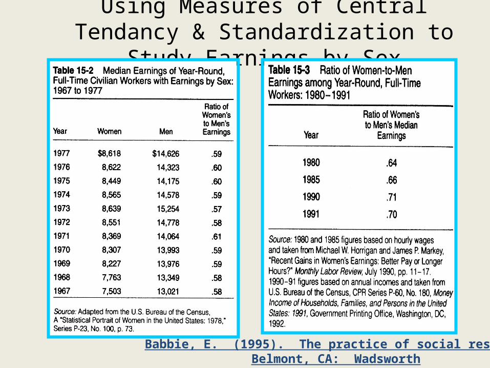
Using Measures of Central Tendancy & Standardization to Study Earnings by Sex
Babbie, E. (1995). The practice of social researchBelmont, CA: Wadsworth

In his book on reading statistical tables, Say it with Figures, Hans Zeisel presents the following data:
Automobile Accidents by Sex
------------------------------------------ Per Cent
Accident Free
Women 68%
(6,950)
Men 56%
(7,080)
------------------------------------------
Automobile Accidents by Sex and Distance Driven
----------------------------------------------------------------------------Distance
Under 10,000 km 10,000 km & Over Per Cent Per CentAccident Free Accident Free
Women 75% 55% (5,035) (1,915)
Men 75% 51% (2,070) (5,010)
----------------------------------------------------------------------------
Women in this study have fewer accidents than men because women tend to drive shorter distances than men, and people
who drive shorter distances tend to have fewer accidents

Discussion of other ways to present same data & talk about observationsDiscussion of other ways to present same data & talk about observations
• styles of presentation of cross-tabulations– Conventions & ease of interpretation of different
ways of calculating percentages and presenting bivariate relations
• Examination of frequency distributions of univariate statistics
• Introduction of third variable• Examples of ways of describing the relationships
in words

Table 1a: Experience of Accidents in the Past Year by Gender of Driver (with column frequencies &
percentages for independent variable)
In this study 68% of the women had been accident free as compared to 56% of the men.
Are women better drivers than men?
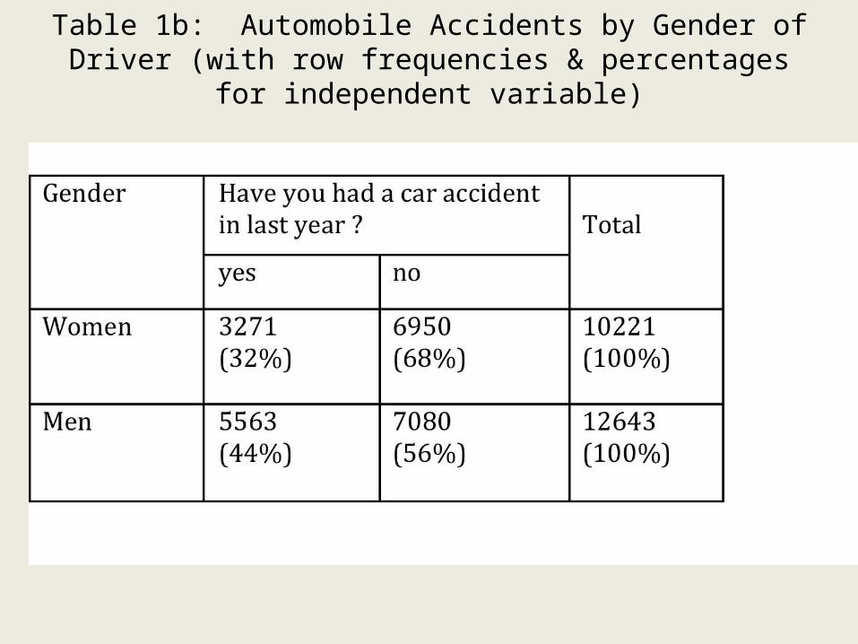
Table 1b: Automobile Accidents by Gender of Driver (with row frequencies & percentages for independent variable)
Commentary
• Based on findings from this survey female drivers are more likely than men to have been accident-free in the past year. The majority of women in the sample (68%) had not had accidents in the past year. A smaller percentage of male drivers (56%) declared they had been accident free in the past year.

Table 2a: Experience of Car Accidents by Gender of Driver (with row frequencies & percentages for dependent variable)
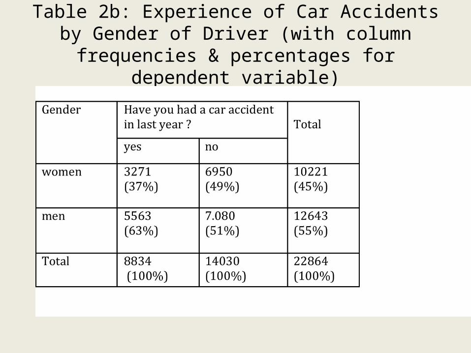
Table 2b: Experience of Car Accidents by Gender of Driver (with column frequencies & percentages for
dependent variable)

Comments on Tables 2a & 2b
• Table 2a and 2b present finding from this survey which indicate that 63% of drivers who experienced at least one car accident in the past year were male and only 37% were female.
• Does this mean men are more likely to experience car accidents than women?

Table 3a: Experience of Car Accidents by Gender of Driver and Distance Driven Annually

Comments on Table 3a• If we control for “distance driven annually” the differences
between the percentage of accident free drivers by gender disappears entirely for people who drive shorter distances annually. In the case of people who drive longer distances annually (10,000 km or more) there is only a small difference between men and women.
• Overall, people who drive shorter distances are more likely to be accident-free than people who drive longer distances, regardless of gender.
•

continued
• People who drove less than 10,000 km annually had the same likelihood of being accident free regardless of gender. Three quarters (75%) of female drivers who drive less than 10,000 km annually remained accident-free and three quarters of male drivers (75%),
continued
• Female drivers who drove longer distances were only slightly more likely than male drivers to have remained accident-free: 55% of the females who drove 10,000k m annually or more had remained accident-free as compared to 51% of male drivers who drove 10,000km or more.
•
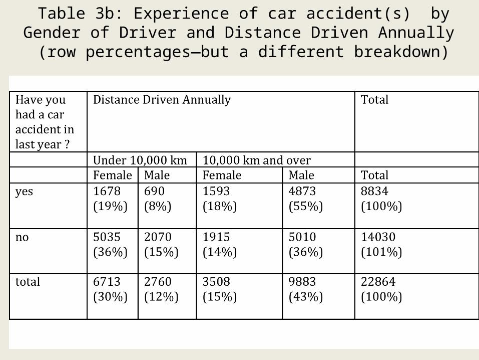
Table 3b: Experience of car accident(s) by Gender of Driver and Distance Driven Annually (row percentages—but a different
breakdown)
Comments on Table 3B
• In this study male drivers who drove longer distances comprise 55% of drivers who had experienced at least one accident in the past year. What would you say about other patterns in this table concerning the trends related to the three variables? (Having at least one accident last year, gender and distance driven?)
•
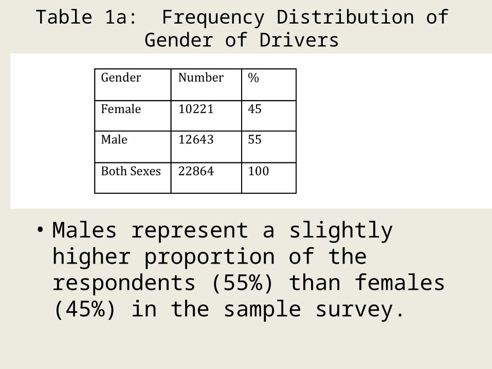
Table 1a: Frequency Distribution of Gender of Drivers
• Males represent a slightly higher proportion of the respondents (55%) than females (45%) in the sample survey.

Table 1b: Frequency Distribution of Drivers with and without accidents in the past year
• The majority of drivers (61%) had not had any accidents in the past year.

Table1c: Frequency Distribution of Distance Driven Annually
• Over half of the drivers in the sample (59%) drive 10,000 km or over annually.
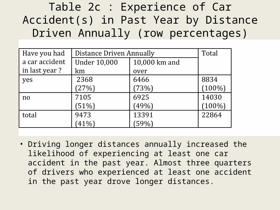
Table 2c : Experience of Car Accident(s) in Past Year by Distance Driven Annually (row percentages)
• Driving longer distances annually increased the likelihood of experiencing at least one car accident in the past year. Almost three quarters of drivers who experienced at least one accident in the past year drove longer distances.
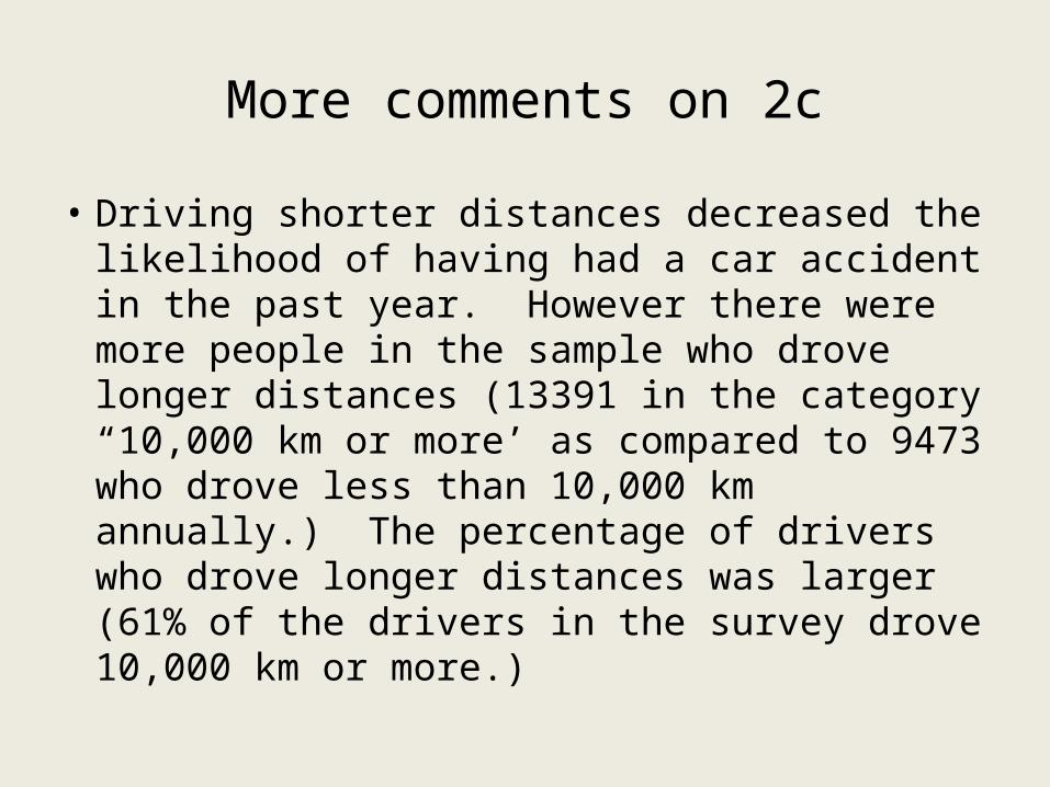
More comments on 2c
• Driving shorter distances decreased the likelihood of having had a car accident in the past year. However there were more people in the sample who drove longer distances (13391 in the category “10,000 km or more’ as compared to 9473 who drove less than 10,000 km annually.) The percentage of drivers who drove longer distances was larger (61% of the drivers in the survey drove 10,000 km or more.)
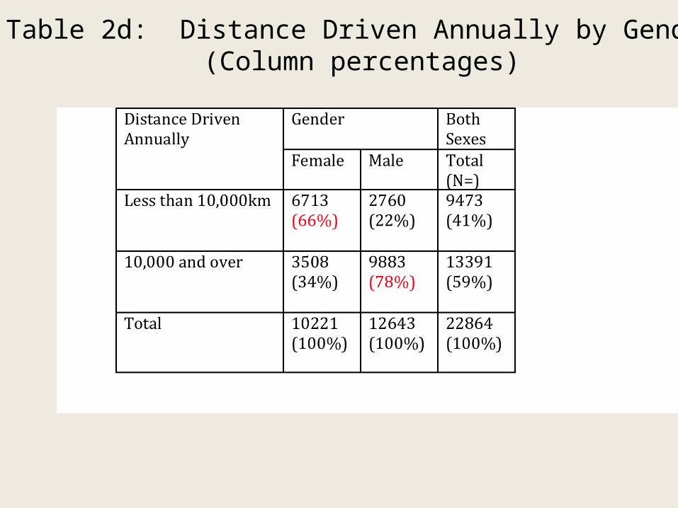
Table 2d: Distance Driven Annually by Gender (Column percentages)

Comments on Table 2d
• Women drivers in the sample drove shorter distances annually than men. Two-thirds of women in the sample (66%) drove less than 10,000 km annually, while 78% of men in the sample drove 10,000 km or more.
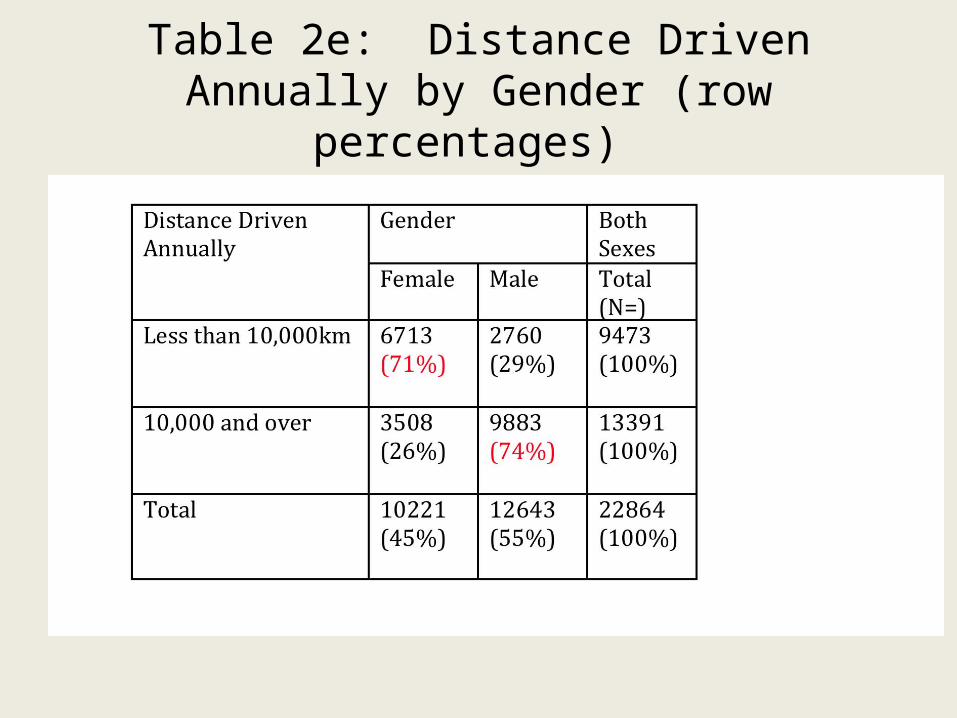
Table 2e: Distance Driven Annually by Gender (row percentages)
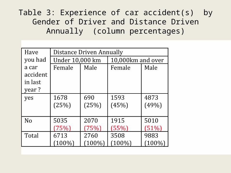
Table 3: Experience of car accident(s) by Gender of Driver and
Distance Driven Annually (column percentages)
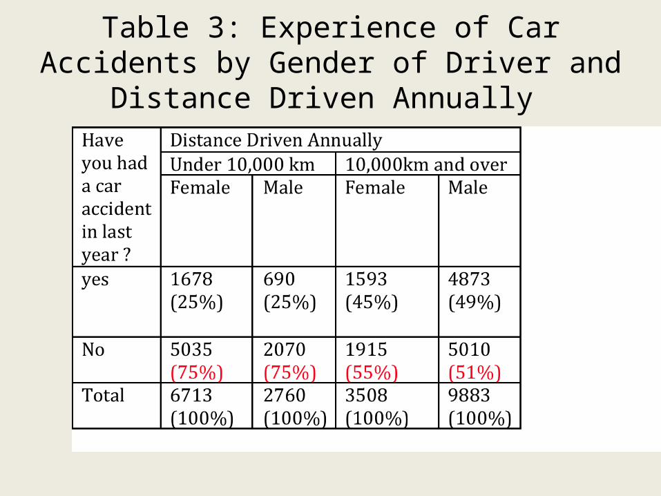
Table 3: Experience of Car Accidents by Gender of Driver and Distance Driven Annually

Comments on 2e
• The majority of drivers who drove less than 10,000 annually were women (71%). Almost three quarters (74%) of drivers who drove 10,000 were male.

Comparison with Ziezel’s TablesAutomobile Accidents by Sex
------------------------------------------ Per Cent
Accident Free
Women 68%
(6,950)
Men 56%
(7,080)
------------------------------------------
Automobile Accidents by Sex and Distance Driven
----------------------------------------------------------------------------Distance
Under 10,000 km 10,000 km & Over Per Cent Per CentAccident Free Accident Free
Women 75% 55% (5,035) (1,915)
Men 75% 51% (2,070) (5,010)
----------------------------------------------------------------------------
Women in this study have fewer accidents than men because women tend to drive shorter distances than men, and people
who drive less frequently tend to have shorter distances.

Ways of Presenting of Percentaged Tables
Table 1. Percentage in support of strike by type of schoolPercent supporting
Type of School Strike
Secondary 60% (800)
Elementary 30% (1000)
__________________________________________________________N = 1800
Serial NumberDescriptive CaptionDependent Variable
IndependentVariable
Variable
Categoriess
One category of dichotomousdependent variable
Marginals for independentvariable
Total Sample
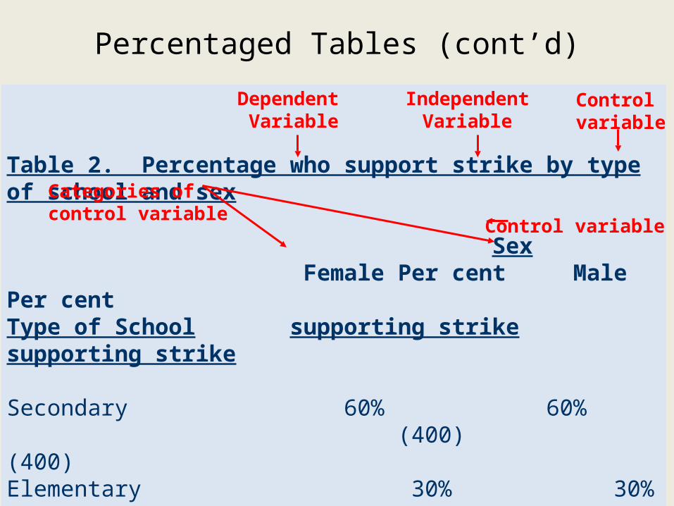
Percentaged Tables (cont’d)
Table 2. Percentage who support strike by type of school and sex
Sex Female Per cent Male Per cent
Type of School supporting strike supporting strike
Secondary 60% 60% (400) (400)
Elementary 30% 30% (900) (100)
__________________________________________________________Female = .30 : Male = .30 N = 1800
Dependent Variable
IndependentVariable
Controlvariable
Control variable
Categories of control variable

Using SPSS to ConstructTables
• General portal to SPSS tutorials online: • http://www.spsstools.net/spss.htm
• crosstabs (two variables) and ‘layering’ (introducing variables)
• http://calcnet.mth.cmich.edu/org/spss/V16_materials/Video_Clips_v16/14crosstabs/14crosstabs.swf

Example of Raw Data Partials & Reading Marginals
Regan, T. (1985). In search of sobriety: Identifying factors contributing to the recovery from alcoholism. Kentville, NS.
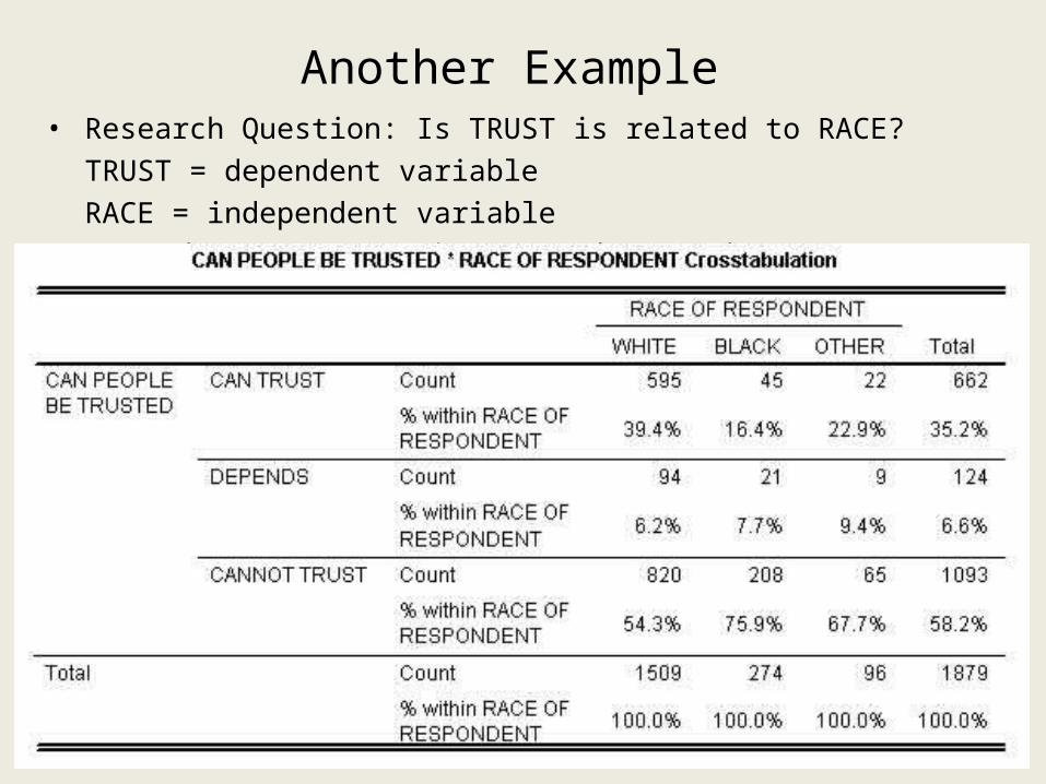
Another Example • Research Question: Is TRUST is related to RACE?
TRUST = dependent variable RACE = independent variable
Source: http://www.ssric.org/trd/text/chapter8
Comments• At first glance, RACE differences appear to be very
important (overall, 58% of those surveyed said people cannot be trusted, but the epsilon statistic -- the difference between the highest and lowest percentage -- is 22). Also note that few Respondents said “Depends” – most had a definite opinion here.

Recoding
• “Let’s do some recoding: RACE should be recoded into a different variable called RACER (Race Recoded). Whites and Blacks will stay the same, but Other is eliminated by recoding it as missing.
• Let’s also recode TRUST into a different variable called TRUSTR to eliminate the “Depends” category. Don’t forget to create new value labels after you recode. Now run the crosstabs for TRUSTR and RACER. Your output should look like Figure 8-4. “
• (See http://www.ssric.org/trd/text/chapter8 for details)
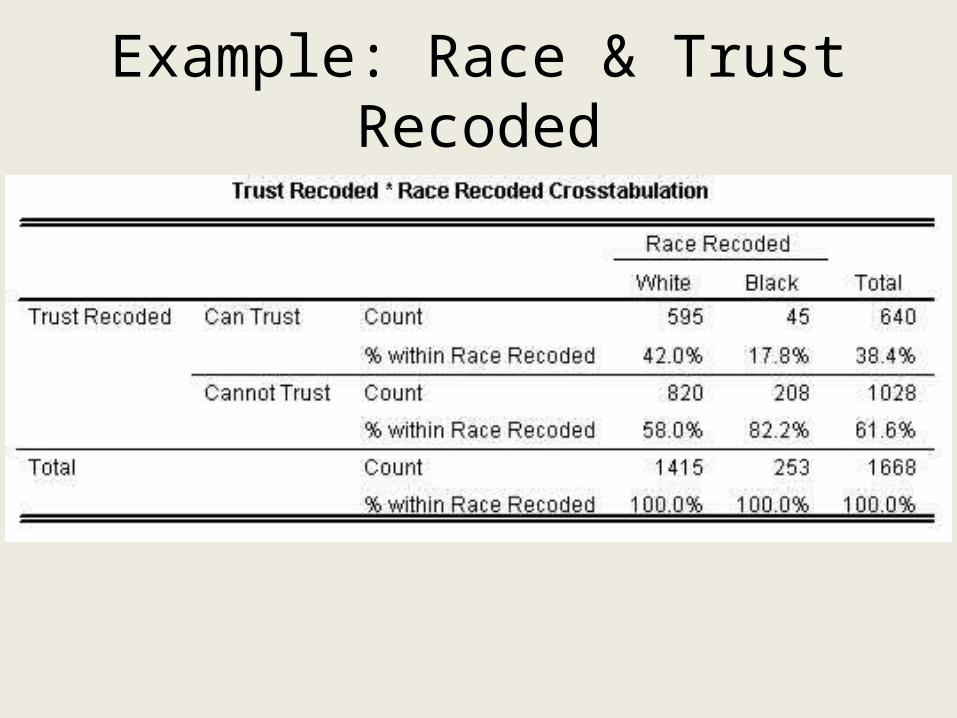
Example: Race & Trust Recoded

Comments• “When "pp", a percentage point difference (epsilon) is this
high, it’s “interesting” (actually, anything higher than 10-12 is interesting) even if you don't yet know whether it is statistically significant. Here you have a pp difference of 24.
• And here’s how you might describe what you’ve found so far: “Although most Respondents (62%) say that other people cannot be trusted, over 80% of the Black respondents said this compared to 58% of the Whites in this sample.”
• Or, “Fewer than one-fifth of Blacks said that people can be trusted, compared to more than two-fifths of Whites.”

Question
• Can you have confidence that race is the causal factor here? While it may indeed be true that race is explanatory, you won't really have confidence in this conclusion until you have failed to account for this variation in any other way.

Introducing a Control Variable
– In the next example EDUC was recoded as EDUC2 into two categories, those with high school or less (0 12 years), and those with more then high school (13+ years). After these recodes, let's see what happens when we do crosstabs
– You still have the two columns of your independent variable (RACER), but you can compare TRUSTR for people who have no college education (0-12 Years) with those who do (13+).

Trust by Race Controlling for Education
Comments
• "Whites are more likely than blacks to think people can be trusted holding education constant (50.1% vs. vs. 31.3% and 32.3% vs. 9.3%). Those with more education are more likely than those with less education to say people can be trusted holding race constant (50.1% vs. 32.3% and 31.3% vs. 9.3%). Both education and race are related to trust of people".

Comments
• “So what is more important, race or years of education? Just as you can’t stop with a crosstab of only two variables when you want to test out your hypotheses, you also can’t stop with just one control variable. Some of the other “major demographic variables” that might explain social differences include sex, social class, income, occupation, marital status, age, political ideology, and religion.”

Discussion of Lab Activities & Demonstration of Accessing Data from
Class Survey


