Block Flow Diagrams (BFD’s) Process Flow Diagrams (PFD’s) Piping and Instrumentation Diagrams (P&ID’s) In general, my work on this type of diagrams has been for private sector entities, and I can’t publish the diagrams on my website. Contact me and I’ll be happy to talk to you about my capabilities in this area. I’ve used the same process for academic projects: two examples are attached. Example 1: PFD for Solar plant using molten salt. Interesting for the use of PFD to characterize light energy: we treated it as a process stream. Example 2: P&ID for Aquifer Storage & Recovery Well.
Transcript
Block Flow Diagrams (BFD’s) Process Flow Diagrams (PFD’s) Piping and Instrumentation Diagrams (P&ID’s) In general, my work on this type of diagrams has been for private sector entities, and I can’t publish the diagrams on my website. Contact me and I’ll be happy to talk to you about my capabilities in this area. I’ve used the same process for academic projects: two examples are attached. Example 1: PFD for Solar plant using molten salt. Interesting for the use of PFD to characterize light energy: we treated it as a process stream. Example 2: P&ID for Aquifer Storage & Recovery Well.
ME4460–SolarEnergy
Final Report
Lisa Denke, Ethan Smith, Jim Rieger, Dustin Collins
May 4, 2014
1 | P a g e
AbstractThis study concerns using solar “power towers” for electrical generation. A block flow diagram and energy balance were made for the entire process, followed by a process flow diagram and preliminary equipment sizing for the thermal storage equipment and receiver heat exchanger. Economics for capital expenditure were estimated.
IntroductionConcentrated solar thermal electrical generation can be accomplished in several ways, including Parabolic Dish Collectors (PDC), Heliostat Field Collectors with a Central Tower, Parabolic Trough Collectors (PTC), and Compound Parabolic Collectors (CPC). Although PTC’s comprise most of the commercial installed base, power tower installations have become commercial and are seeing increasing use, and it is these plants that are referred to as Concentrated Solar Power (CSP) plants. CSP plants are challenging to design, permit, construct, build, and operate. A first step is to develop an understanding of the systems and costs involved. This study is an effort to accomplish that goal.
ApproachtoProjectA standard process engineering approach was taken, in the following steps:
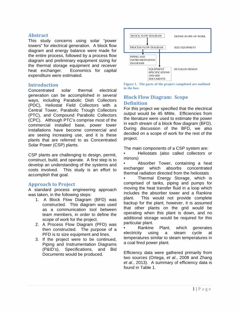
1. A Block Flow Diagram (BFD) was constructed. This diagram was used as a communication tool between team members, in order to define the scope of work for the project.
2. A Process Flow Diagram (PFD) was then constructed. The purpose of a PFD is to size equipment and lines.
3. If the project were to be continued, Piping and Instrumentation Diagrams (P&ID’s), Specifications, and Bid Documents would be produced.
Figure 1. The parts of the project completed are outlined in the box.
BlockFlowDiagram:ScopeDefinitionFor this project we specified that the electrical output would be 45 MWe. Efficiencies from the literature were used to estimate the power in each stream of a block flow diagram (BFD). During discussion of the BFD, we also decided on a scope of work for the rest of the project. The main components of a CSP system are: • Heliostats (also called collectors or mirrors) • Absorber Tower, containing a heat exchanger which absorbs concentrated thermal radiation directed from the heliostats • Thermal Energy Storage, which is comprised of tanks, piping and pumps for moving the heat transfer fluid in a loop which includes the absorber tower and a Rankine plant. This would not provide complete backup for the plant, however, it is assumed that other plants on the grid would be operating when this plant is down, and no additional storage would be required for this particular plant. • Rankine Plant, which generates electricity using a steam cycle at temperatures similar to steam temperatures in a coal fired power plant. Efficiency data were gathered primarily from two sources (Ortega, et al., 2008 and Zhang et al., 2013). A summary of efficiency data is found in Table 1.
2 | P a g e
Table 1. Efficiency for CSP plant systems.
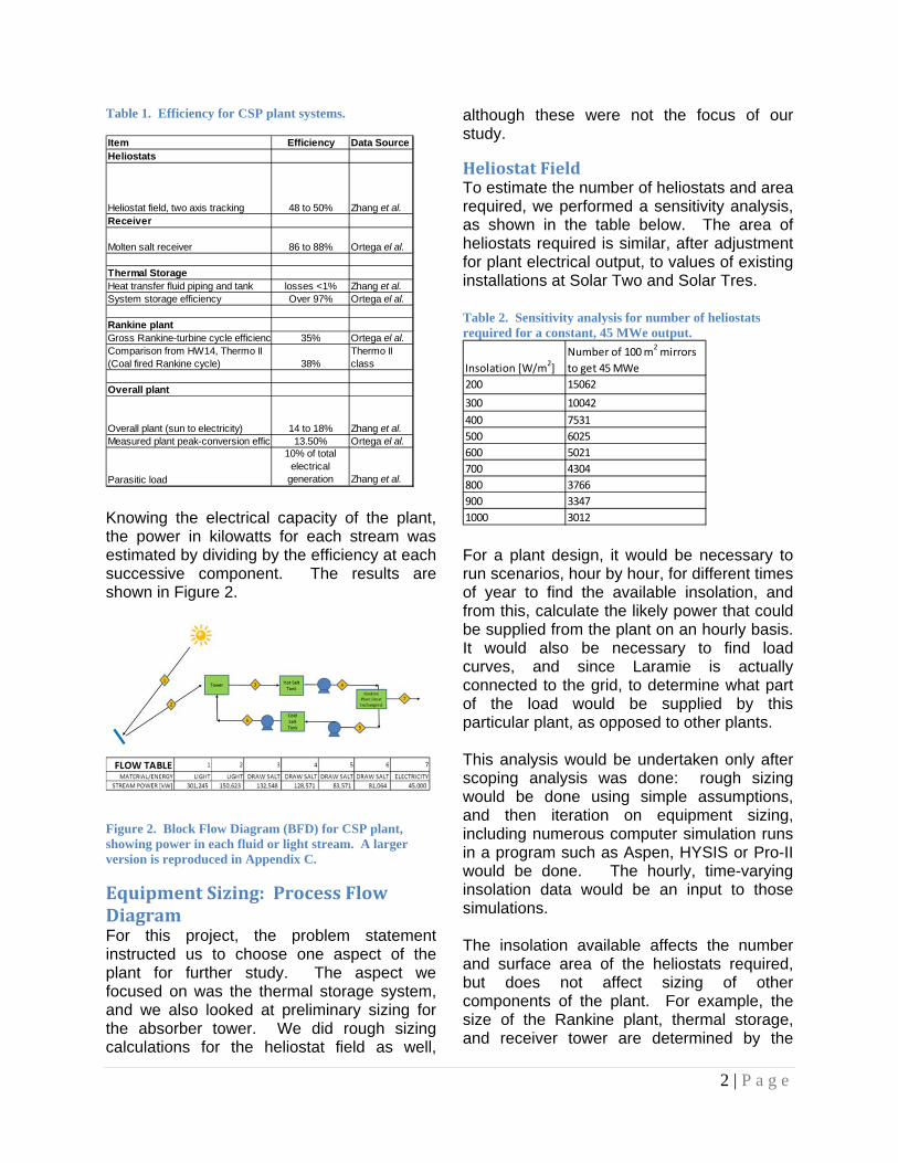
Knowing the electrical capacity of the plant, the power in kilowatts for each stream was estimated by dividing by the efficiency at each successive component. The results are shown in Figure 2.
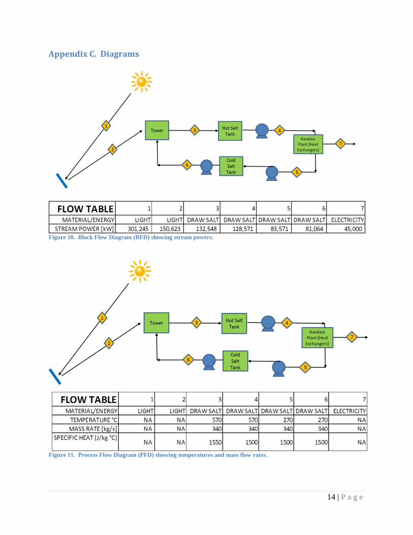
Figure 2. Block Flow Diagram (BFD) for CSP plant, showing power in each fluid or light stream. A larger version is reproduced in Appendix C.
EquipmentSizing:ProcessFlowDiagramFor this project, the problem statement instructed us to choose one aspect of the plant for further study. The aspect we focused on was the thermal storage system, and we also looked at preliminary sizing for the absorber tower. We did rough sizing calculations for the heliostat field as well,
although these were not the focus of our study.
HeliostatFieldTo estimate the number of heliostats and area required, we performed a sensitivity analysis, as shown in the table below. The area of heliostats required is similar, after adjustment for plant electrical output, to values of existing installations at Solar Two and Solar Tres. Table 2. Sensitivity analysis for number of heliostats required for a constant, 45 MWe output.
For a plant design, it would be necessary to run scenarios, hour by hour, for different times of year to find the available insolation, and from this, calculate the likely power that could be supplied from the plant on an hourly basis. It would also be necessary to find load curves, and since Laramie is actually connected to the grid, to determine what part of the load would be supplied by this particular plant, as opposed to other plants. This analysis would be undertaken only after scoping analysis was done: rough sizing would be done using simple assumptions, and then iteration on equipment sizing, including numerous computer simulation runs in a program such as Aspen, HYSIS or Pro-II would be done. The hourly, time-varying insolation data would be an input to those simulations. The insolation available affects the number and surface area of the heliostats required, but does not affect sizing of other components of the plant. For example, the size of the Rankine plant, thermal storage, and receiver tower are determined by the
Item Efficiency Data SourceHeliostats
Heliostat field, two axis tracking 48 to 50% Zhang et al.Receiver
Molten salt receiver 86 to 88% Ortega el al.
Thermal StorageHeat transfer fluid piping and tank losses <1% Zhang et al.System storage efficiency Over 97% Ortega el al.
Rankine plantGross Rankine-turbine cycle efficienc 35% Ortega el al.Comparison from HW14, Thermo II (Coal fired Rankine cycle) 38%
Thermo II class
Overall plant
Overall plant (sun to electricity) 14 to 18% Zhang et al.Measured plant peak-conversion effici 13.50% Ortega el al.
Parasitic load
10% of total electrical
generation Zhang et al.
Insolation [W/m2]
Number of 100 m2 mirrors
to get 45 MWe
200 15062
300 10042
400 7531
500 6025
600 5021
700 4304
800 3766
900 3347
1000 3012
3 | P a g e
required electrical output, not by the available insolation. The insolation is important, because it determines the cost of the heliostat field, and would likely limit the economics.
ThermalStorageSystemSince the sun does not provide energy to the plant all the time, it is necessary to store energy to run the plant during times that the sun is not shining. It is common to use the fluid, such as molten salt, to store heat. As shown in the block flow diagram, relatively cold liquid salt is heated by pumping it through the absorber tower, and then the hot salt is held in a tank until needed to generate electricity.
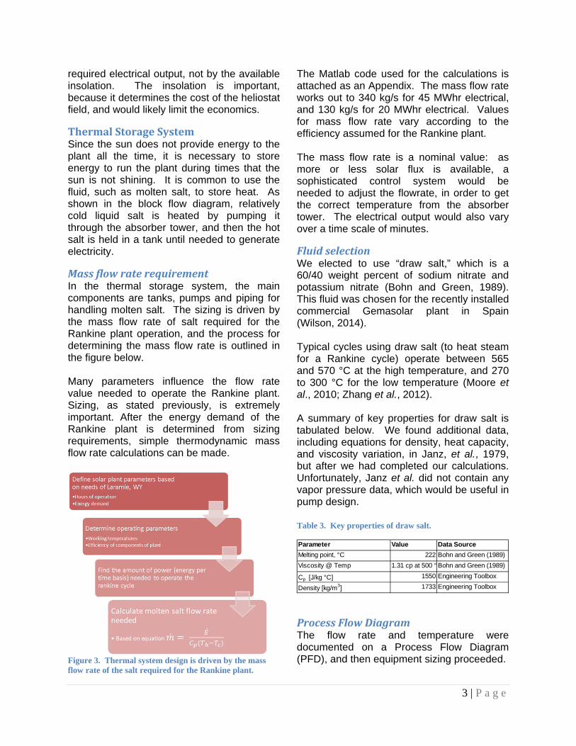
MassflowraterequirementIn the thermal storage system, the main components are tanks, pumps and piping for handling molten salt. The sizing is driven by the mass flow rate of salt required for the Rankine plant operation, and the process for determining the mass flow rate is outlined in the figure below. Many parameters influence the flow rate value needed to operate the Rankine plant. Sizing, as stated previously, is extremely important. After the energy demand of the Rankine plant is determined from sizing requirements, simple thermodynamic mass flow rate calculations can be made.
Figure 3. Thermal system design is driven by the mass flow rate of the salt required for the Rankine plant.
The Matlab code used for the calculations is attached as an Appendix. The mass flow rate works out to 340 kg/s for 45 MWhr electrical, and 130 kg/s for 20 MWhr electrical. Values for mass flow rate vary according to the efficiency assumed for the Rankine plant. The mass flow rate is a nominal value: as more or less solar flux is available, a sophisticated control system would be needed to adjust the flowrate, in order to get the correct temperature from the absorber tower. The electrical output would also vary over a time scale of minutes.
FluidselectionWe elected to use “draw salt,” which is a 60/40 weight percent of sodium nitrate and potassium nitrate (Bohn and Green, 1989). This fluid was chosen for the recently installed commercial Gemasolar plant in Spain (Wilson, 2014). Typical cycles using draw salt (to heat steam for a Rankine cycle) operate between 565 and 570 °C at the high temperature, and 270 to 300 °C for the low temperature (Moore et al., 2010; Zhang et al., 2012). A summary of key properties for draw salt is tabulated below. We found additional data, including equations for density, heat capacity, and viscosity variation, in Janz, et al., 1979, but after we had completed our calculations. Unfortunately, Janz et al. did not contain any vapor pressure data, which would be useful in pump design. Table 3. Key properties of draw salt.
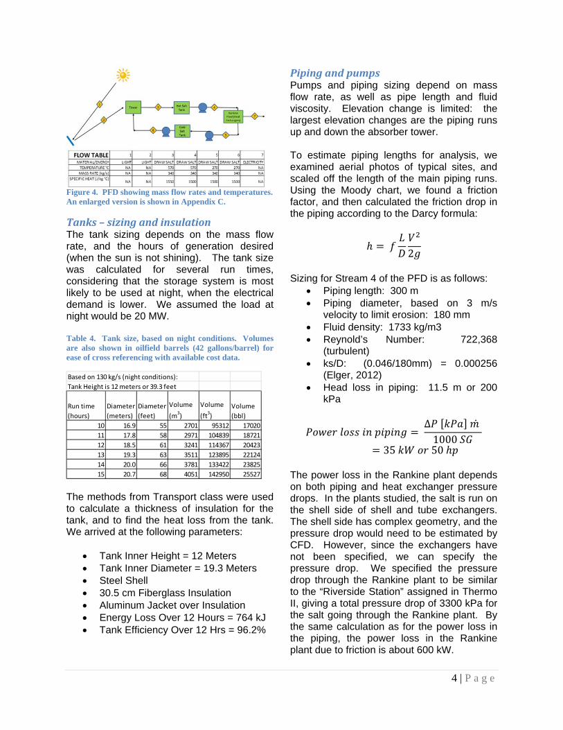
ProcessFlowDiagramThe flow rate and temperature were documented on a Process Flow Diagram (PFD), and then equipment sizing proceeded.
Parameter Value Data Source
Melting point, °C 222 Bohn and Green (1989)
Viscosity @ Temp 1.31 cp at 500 ° Bohn and Green (1989)
Cp [J/kg °C] 1550 Engineering Toolbox
Density [kg/m3] 1733 Engineering Toolbox
4 | P a g e
Figure 4. PFD showing mass flow rates and temperatures. An enlarged version is shown in Appendix C.
Tanks–sizingandinsulationThe tank sizing depends on the mass flow rate, and the hours of generation desired (when the sun is not shining). The tank size was calculated for several run times, considering that the storage system is most likely to be used at night, when the electrical demand is lower. We assumed the load at night would be 20 MW. Table 4. Tank size, based on night conditions. Volumes are also shown in oilfield barrels (42 gallons/barrel) for ease of cross referencing with available cost data.
The methods from Transport class were used to calculate a thickness of insulation for the tank, and to find the heat loss from the tank. We arrived at the following parameters:
Tank Inner Height = 12 Meters Tank Inner Diameter = 19.3 Meters Steel Shell 30.5 cm Fiberglass Insulation Aluminum Jacket over Insulation Energy Loss Over 12 Hours = 764 kJ Tank Efficiency Over 12 Hrs = 96.2%
PipingandpumpsPumps and piping sizing depend on mass flow rate, as well as pipe length and fluid viscosity. Elevation change is limited: the largest elevation changes are the piping runs up and down the absorber tower. To estimate piping lengths for analysis, we examined aerial photos of typical sites, and scaled off the length of the main piping runs. Using the Moody chart, we found a friction factor, and then calculated the friction drop in the piping according to the Darcy formula:
2
Sizing for Stream 4 of the PFD is as follows:
Piping length: 300 m Piping diameter, based on 3 m/s
velocity to limit erosion: 180 mm Fluid density: 1733 kg/m3 Reynold’s Number: 722,368
(turbulent) ks/D: (0.046/180mm) = 0.000256
(Elger, 2012) Head loss in piping: 11.5 m or 200
kPa
∆ 1000
35 50 The power loss in the Rankine plant depends on both piping and heat exchanger pressure drops. In the plants studied, the salt is run on the shell side of shell and tube exchangers. The shell side has complex geometry, and the pressure drop would need to be estimated by CFD. However, since the exchangers have not been specified, we can specify the pressure drop. We specified the pressure drop through the Rankine plant to be similar to the “Riverside Station” assigned in Thermo II, giving a total pressure drop of 3300 kPa for the salt going through the Rankine plant. By the same calculation as for the power loss in the piping, the power loss in the Rankine plant due to friction is about 600 kW.
Based on 130 kg/s (night conditions):
Tank Height is 12 meters or 39.3 feet
Run time
(hours)
Diameter
(meters)
Diameter
(feet)
Volume
(m3)
Volume
(ft3)
Volume
(bbl)
10 16.9 55 2701 95312 17020
11 17.8 58 2971 104839 18721
12 18.5 61 3241 114367 20423
13 19.3 63 3511 123895 22124
14 20.0 66 3781 133422 23825
15 20.7 68 4051 142950 25527
5 | P a g e
It would be possible to install a separate pump in Stream 5 downstream of the Rankine Plant. The power added by that pump would be around 120 kW. The power added by pumps in streams 4 and 5 is added together in the table below.
Figure 5. Pumping hydraulic power required hot salt pump(s).
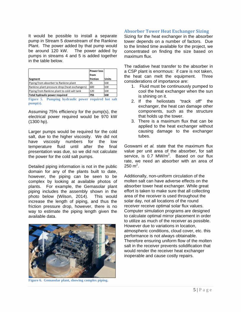
Assuming 75% efficiency for the pump(s), the electrical power required would be 970 kW (1300 hp). Larger pumps would be required for the cold salt, due to the higher viscosity. We did not have viscosity numbers for the low temperature fluid until after the final presentation was due, so we did not calculate the power for the cold salt pumps. Detailed piping information is not in the public domain for any of the plants built to date, however, the piping can be seen to be complex by looking at available photos of plants. For example, the Gemasolar plant piping includes the assembly shown in the photo below (Wilson, 2014). This would increase the length of piping, and thus the friction pressure drop, however, there is no way to estimate the piping length given the available data.
AbsorberTowerHeatExchangerSizingSizing for the heat exchanger in the absorber tower depends on a number of factors. Due to the limited time available for the project, we concentrated on finding the size based on maximum flux. The radiative heat transfer to the absorber in a CSP plant is enormous: if care is not taken, the heat can melt the equipment. Three considerations of importance are:
1. Fluid must be continuously pumped to cool the heat exchanger when the sun is shining on it.
2. If the heliostats “track off” the exchanger, the heat can damage other components, such as the structure that holds up the tower.
3. There is a maximum flux that can be applied to the heat exchanger without causing damage to the exchanger tubes.
Goswami et al. state that the maximum flux value per unit area of the absorber, for salt service, is 0.7 MW/m2. Based on our flux rate, we need an absorber with an area of 250 m2. Additionally, non-uniform circulation of the molten salt can have adverse effects on the absorber tower heat exchanger. While great effort is taken to make sure that all collecting area of the receiver is used throughout the solar day, not all locations of the round receiver receive optimal solar flux values. Computer simulation programs are designed to calculate optimal mirror placement in order to utilize as much of the receiver as possible. However due to variations in location, atmospheric conditions, cloud cover, etc. this performance is not always obtainable. Therefore ensuring uniform flow of the molten salt in the receiver prevents solidification that would render the receiver heat exchanger inoperable and cause costly repairs.
Segment
Power loss
from
friction Units
Piping from absorber to Rankine plant 35 kW
Rankine plant pressure drop (heat exchangers) 600 kW
Piping from Rankine plant to cold salt tank 120 kW
Total hydraulic power required 755 kW
6 | P a g e
EconomicsIdeally, one would like to have three types of economics data:
1. Capital cost 2. Operating cost 3. Revenue
Economics “numbers” are easy to obtain for CSP installations. However, the data are often missing crucial information, such as the scope associated with a given cost. We concentrated on getting accurate data, at the expense of getting “complete” data. We did find capital cost data that seem consistent enough to include. We used capital cost data of several types:
1. Ballpark data in terms of $/kW 2. Costs for major subsystems in the
plant a. Heliostat field b. Steam generator c. Thermal storage d. Absorber
3. Costs for tanks, which are an item within the thermal storage subsystem
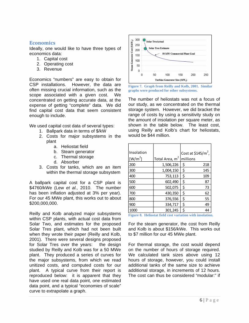
A ballpark capital cost for a CSP plant is $4760/kWe (Lew et al., 2010. The number has been inflation adjusted at 3% per year). For our 45 MWe plant, this works out to about $200,000,000. Reilly and Kolb analyzed major subsystems within CSP plants, with actual cost data from Solar Two, and estimates for the proposed Solar Tres plant, which had not been built when they wrote their paper (Reilly and Kolb, 2001). There were several designs proposed for Solar Tres over the years: the design studied by Reilly and Kolb was for a 50 MWe plant. They produced a series of curves for the major subsystems, from which we read unitized costs, and computed costs for our plant. A typical curve from their report is reproduced below: it is apparent that they have used one real data point, one estimated data point, and a typical “economies of scale” curve to extrapolate a graph.
Figure 7. Graph from Reilly and Kolb, 2001. Similar graphs were produced for other subsystems.
The number of heliostats was not a focus of our study, as we concentrated on the thermal storage system. However, we did bracket the range of costs by using a sensitivity study on the amount of insolation per square meter, as shown in the table below. The least cost, using Reilly and Kolb’s chart for heliostats, would be $44 million.
Figure 8. Heliostat field cost variation with insolation.
For the steam generator, the cost from Reilly and Kolb is about $156/kWe. This works out to $7 million for our 45 MWe plant. For thermal storage, the cost would depend on the number of hours of storage required. We calculated tank sizes above using 12 hours of storage, however, you could install additional tanks of the same size to achieve additional storage, in increments of 12 hours. The cost can thus be considered “modular:” if
Insolation
[W/m2] Total Area, m
2Cost at $145/m
2,
millions
200 1,506,226 218$
300 1,004,150 145$
400 753,113 109$
500 602,490 87$
600 502,075 73$
700 430,350 62$
800 376,556 55$
900 334,717 49$
1000 301,245 44$
7 | P a g e
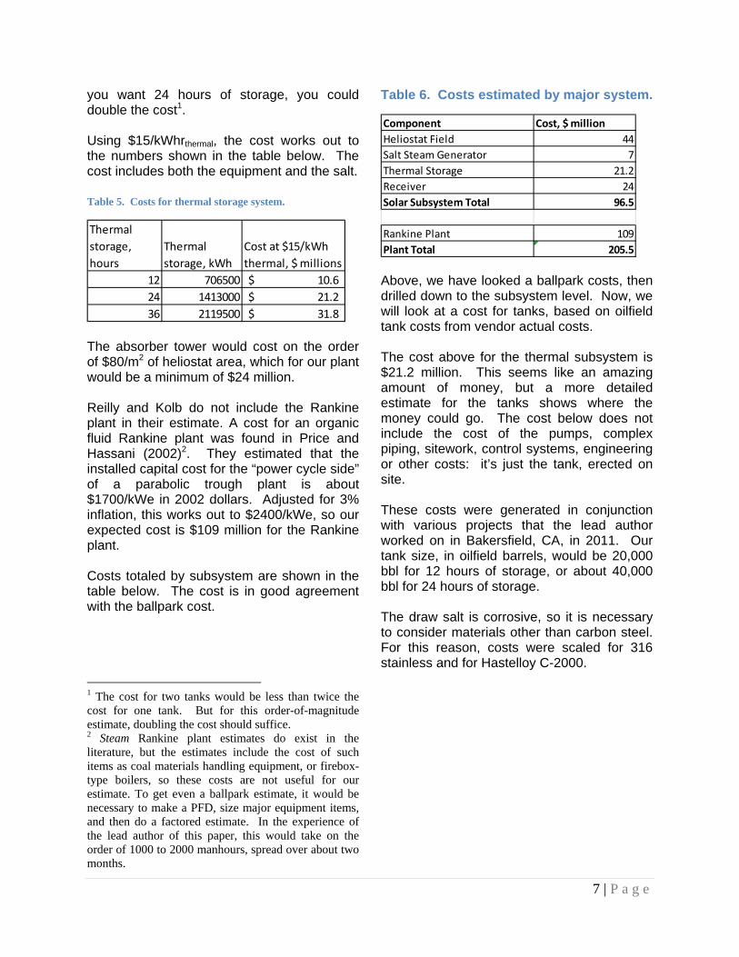
you want 24 hours of storage, you could double the cost1. Using $15/kWhrthermal, the cost works out to the numbers shown in the table below. The cost includes both the equipment and the salt. Table 5. Costs for thermal storage system.
The absorber tower would cost on the order of $80/m2 of heliostat area, which for our plant would be a minimum of $24 million. Reilly and Kolb do not include the Rankine plant in their estimate. A cost for an organic fluid Rankine plant was found in Price and Hassani (2002)2. They estimated that the installed capital cost for the “power cycle side” of a parabolic trough plant is about $1700/kWe in 2002 dollars. Adjusted for 3% inflation, this works out to $2400/kWe, so our expected cost is $109 million for the Rankine plant. Costs totaled by subsystem are shown in the table below. The cost is in good agreement with the ballpark cost.
1 The cost for two tanks would be less than twice the cost for one tank. But for this order-of-magnitude estimate, doubling the cost should suffice. 2 Steam Rankine plant estimates do exist in the literature, but the estimates include the cost of such items as coal materials handling equipment, or firebox-type boilers, so these costs are not useful for our estimate. To get even a ballpark estimate, it would be necessary to make a PFD, size major equipment items, and then do a factored estimate. In the experience of the lead author of this paper, this would take on the order of 1000 to 2000 manhours, spread over about two months.
Table 6. Costs estimated by major system.
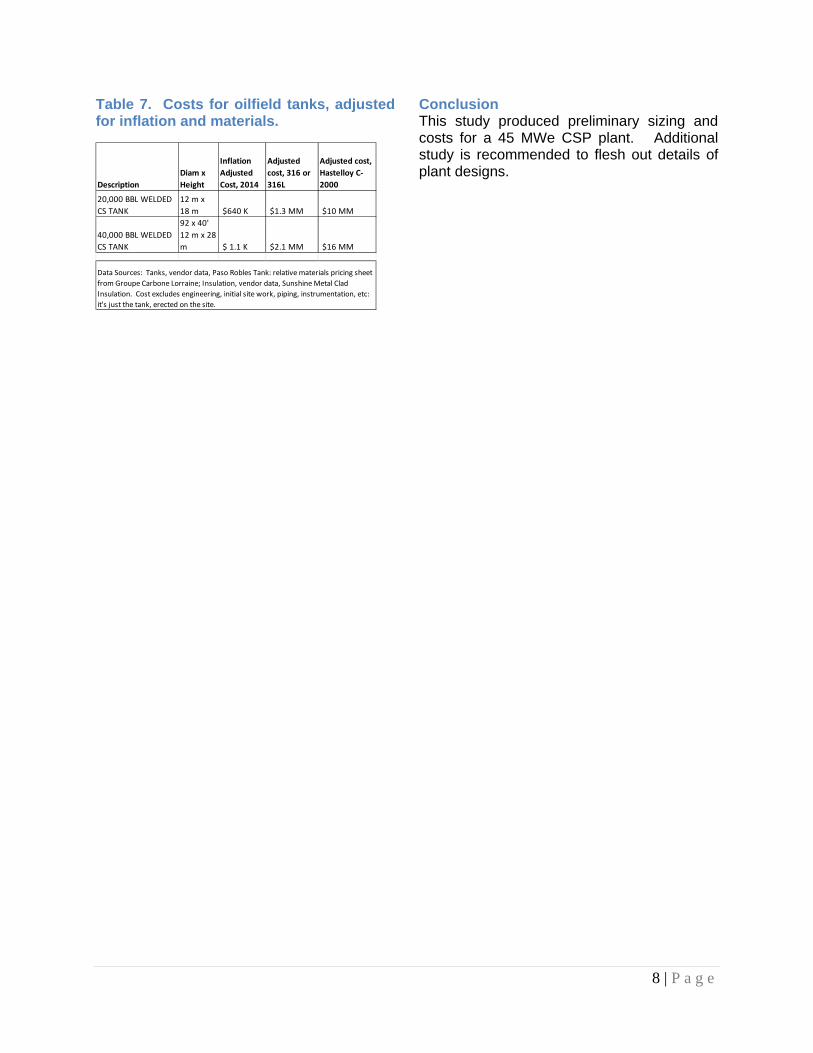
Above, we have looked a ballpark costs, then drilled down to the subsystem level. Now, we will look at a cost for tanks, based on oilfield tank costs from vendor actual costs. The cost above for the thermal subsystem is $21.2 million. This seems like an amazing amount of money, but a more detailed estimate for the tanks shows where the money could go. The cost below does not include the cost of the pumps, complex piping, sitework, control systems, engineering or other costs: it’s just the tank, erected on site. These costs were generated in conjunction with various projects that the lead author worked on in Bakersfield, CA, in 2011. Our tank size, in oilfield barrels, would be 20,000 bbl for 12 hours of storage, or about 40,000 bbl for 24 hours of storage. The draw salt is corrosive, so it is necessary to consider materials other than carbon steel. For this reason, costs were scaled for 316 stainless and for Hastelloy C-2000.
Thermal
storage,
hours
Thermal
storage, kWh
Cost at $15/kWh
thermal, $ millions
12 706500 10.6$
24 1413000 21.2$
36 2119500 31.8$
Component Cost, $ million
Heliostat Field 44
Salt Steam Generator 7
Thermal Storage 21.2
Receiver 24
Solar Subsystem Total 96.5
Rankine Plant 109
Plant Total 205.5
8 | P a g e
Table 7. Costs for oilfield tanks, adjusted for inflation and materials.
Conclusion This study produced preliminary sizing and costs for a 45 MWe CSP plant. Additional study is recommended to flesh out details of plant designs. Description
from Groupe Carbone Lorraine; Insulation, vendor data, Sunshine Metal Clad
Insulation. Cost excludes engineering, initial site work, piping, instrumentation, etc:
it's just the tank, erected on the site.
9 | P a g e
References Bohn, M.S., and Green, H.J. Heat Transfer in Molten Salt Direct Absorption Receivers. Solar Energy Vol. 42, No. 1, pp. 57 – 66, 1989. Boubault, A., Claudet, B., Faugeroux, O., and Olalde, G. Study of the Accelerated Aging of a Two-Layer Material Used in High-Concentration Solar Receivers. Powerpoint presentation presented at WREF 2012. Accessed March 13, 2012 at https://ases.conference-services.net/resources/252/2859/pres/SOLAR2012_0103_presentation.pdf Elger, D.F., Williams, B.C., Crowe, C.T., and Roberson, J.A. Engineering Fluid Mechanics. John Wiley and Sons, Hoboken, NJ. 2012. Goswami, D.Y., Kreith, F., and Kreider, J.F. Principles of Solar Engineering. Taylor and Francis, Philadelphia, PA, 2000. Groupe Carbone Lorraine. Relative Materials Pricing Sheet. Oxnard, CA. 2004. See Appendix E for this document. Heat Storage in Materials. http://www.engineeringtoolbox.com/sensible-heat-storage-d_1217.html, accessed April 16, 2014. Bergman, T.L., Lavine, A.S., Incropera, F.P., and Dewitt, D.P. Fundamentals of Heat and Mass Transfer. John Wiley and Sons, Hoboken, NJ. 2011. Janz, G.J., Allen, C.B., Bansal, N.P., Murphy, R.M., and Tomkins, R.P.T.. Physical Properties Data Compilations Relevant to Energy Storage. National Bureau of Standards, Washington, D.C. 1979. Lew, D., Brinkman, G., Ibanez, E., Florita, A., Heaney, M., Hodge, B.M., Hummon, M., Stark, G., King, J., Lefton, S.A., Kumar, N., Agan, D., Jordan, G., and Venkataraman, S. Western Wind and Solar Integration Study: Executive Summary. The National Renewable Energy Laboratory, 2010. Mills, D., Lievre, P., Schramek, P., and Stein, W. Design of the Heliostat Field of the CSIRO Solar Tower. Journal of Solar Energy Engineering. Volume 131, Issue 2. Assessed March 15, 2014. http://solarenergyengineering.asmedigitalcollection.asme.org/article.aspx?articleid=1458177 Moore, R., Vernon, M., Ho, C.K., Siegel, N.P., and Kolb, G.J. Design Considerations for Concentrating Solar Power Tower Systems Employing Molten Salt. Sandia National Laboratories, 2010. Ortega, J.I., Burgaleta, J.I, and Téllez, F.M. Central Receiver System Solar Power Plant Using Molten Salt as Heat Transfer Fluid. J. Sol Energy Eng. 130(2), 024501 (Feb 12, 2008). Pacheco, J. Molten Nitrate Salt for Thermal Storage with Parabolic Troughs. Powerpoint presentation presented at 1999 Parabolic Trough Technology Workshop. National Renewable Energy Laboratory. Accessed March 8, 2014 at http://www.nrel.gov/csp/troughnet/wkshp_1999.html
10 | P a g e
Public Service Company of Oklahoma. Heat Balance, Maximum Guaranteed Flow. Riverside Station - Unit 1. Unknown Date. This document is reproduced in Appendix E. Reilly, H.E., and Kolb, G.J. An Evaluation of Molten-Salt Power Towers Including Results of the Solar Two Project. Sandia National Laboratories, 2001. Sargent and Lundy LLC Consulting Group. Assessment of Parabolic Trough and Power Tower Solar Technology Cost and Performance Forecasts. National Renewable Energy Laboratory, 2003. Sener corporation. Undated. CPV & CSP Two Axes Solar Tracker. Datasheet from Sener corporation. Accessed March 13, 2014 at http://www.sener-power-process.com/EPORTAL_DOCS/GENERAL/SENERV2/DOC-cw499d8e0908599/CPVCSPtwoaxessolartracker.pdf. Tyner, C., Sutherland, P., and Gould, W. Solar Two: A Molten Salt Power Tower Demonstration. Stanford, 1995. Accessed March 9, 2014 at http://large.stanford.edu/publications/coal/references/docs/1605696.pdf Wilson, N. 20MW Gemasolar Plant: Elegant, But Pricey. The Energy Collective. Accessed March 10, 2014 at http://theenergycollective.com/nathan-wilson/58791/20mw-gemasolar-plant-elegant-pricey Zhang, H.L, Baeyens, J., Degréve, J. and Cacéres, G. Concentrated solar power plants: Review and design methodology. Renewable and Sustainable Energy Reviews 22 (2013) 466-481.
11 | P a g e
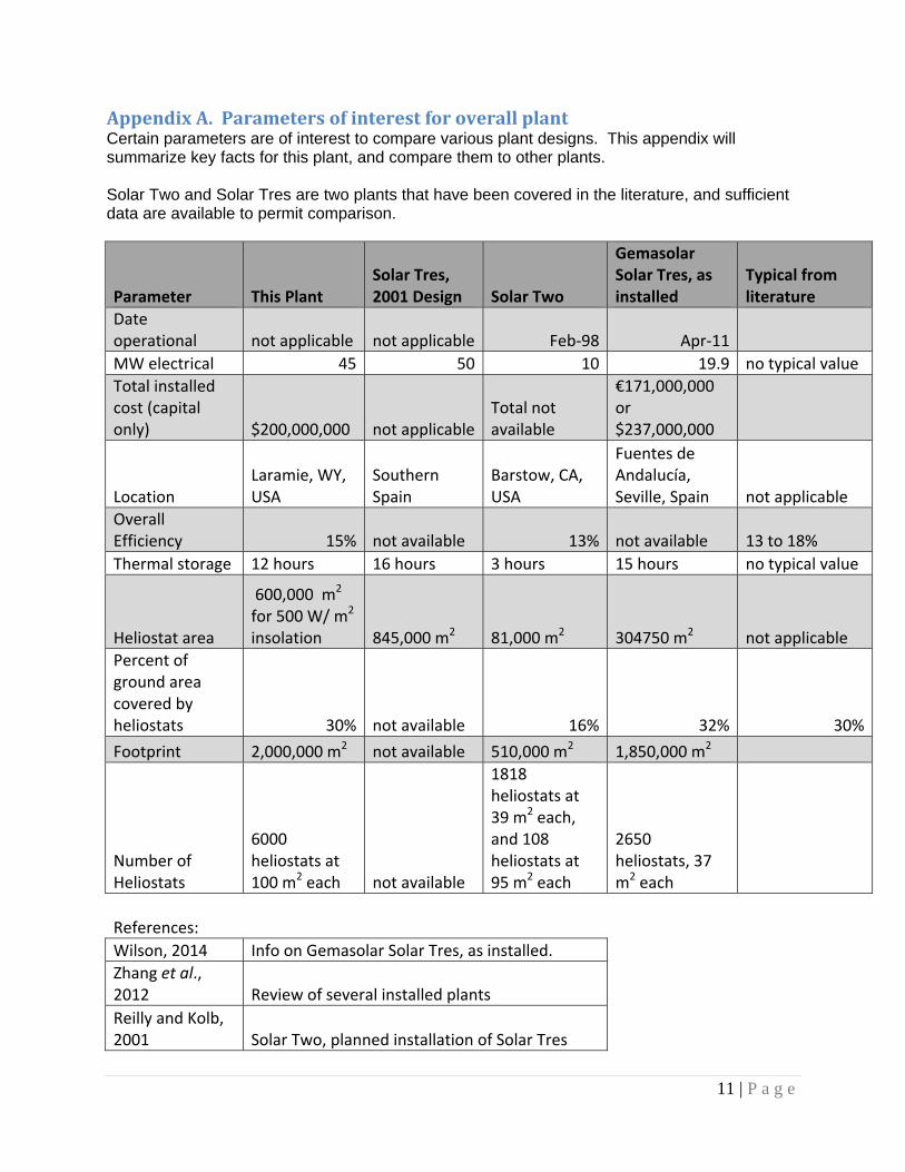
AppendixA.ParametersofinterestforoverallplantCertain parameters are of interest to compare various plant designs. This appendix will summarize key facts for this plant, and compare them to other plants. Solar Two and Solar Tres are two plants that have been covered in the literature, and sufficient data are available to permit comparison.
Parameter This Plant Solar Tres, 2001 Design Solar Two
Gemasolar Solar Tres, as installed
Typical from literature
Date operational not applicable not applicable Feb‐98 Apr‐11
MW electrical 45 50 10 19.9 no typical value
Total installed cost (capital only) $200,000,000 not applicable
Total not available
€171,000,000 or $237,000,000
Location Laramie, WY, USA
Southern Spain
Barstow, CA, USA
Fuentes de Andalucía, Seville, Spain not applicable
Overall Efficiency 15% not available 13% not available 13 to 18%
Thermal storage 12 hours 16 hours 3 hours 15 hours no typical value
Heliostat area
600,000 m2 for 500 W/ m2
insolation 845,000 m2 81,000 m2 304750 m2 not applicable
Percent of ground area covered by heliostats 30% not available 16% 32% 30%
Footprint 2,000,000 m2 not available 510,000 m2 1,850,000 m2
Number of Heliostats
6000 heliostats at 100 m2 each not available
1818 heliostats at 39 m2 each, and 108 heliostats at 95 m2 each
2650 heliostats, 37 m2 each
References:
Wilson, 2014 Info on Gemasolar Solar Tres, as installed.
Zhang et al., 2012 Review of several installed plants
Reilly and Kolb, 2001 Solar Two, planned installation of Solar Tres
12 | P a g e
Notes:
Total installed cost of Solar Two is not readily available. However, since the plant was installed, the technologies have advanced to the point that the cost may not be useful anyway.
Solar Tres plant underwent several design revisions which are covered in the literature. It is difficult to sort out which design revision is referred to in various papers. The column for "Solar Tres, 2001 Design" contains data from Reilly and Kolb, 2001. These data are proposed, as opposed to actual.
PlantsizeAs the plants have a large footprint, the size is a topic of interest. We found the size of our plant could stretch roughly from UW’s Classroom Building to the football stadium. If you look on Google Maps, there will be a scale bar. It will automatically adjust as you zoom in and out. We zoomed in on the Gemasolar Plant until the scale bar showed 200 meters, and then zoomed in on the UW campus to the same scale. Putting the two aerial photos side by side shows that our sizing is of the right order of magnitude.
Figure 9. Gemasolar plant (left) and University of Wyoming campus (right). Our proposed plant is roughly the size of the main campus.
13 | P a g e
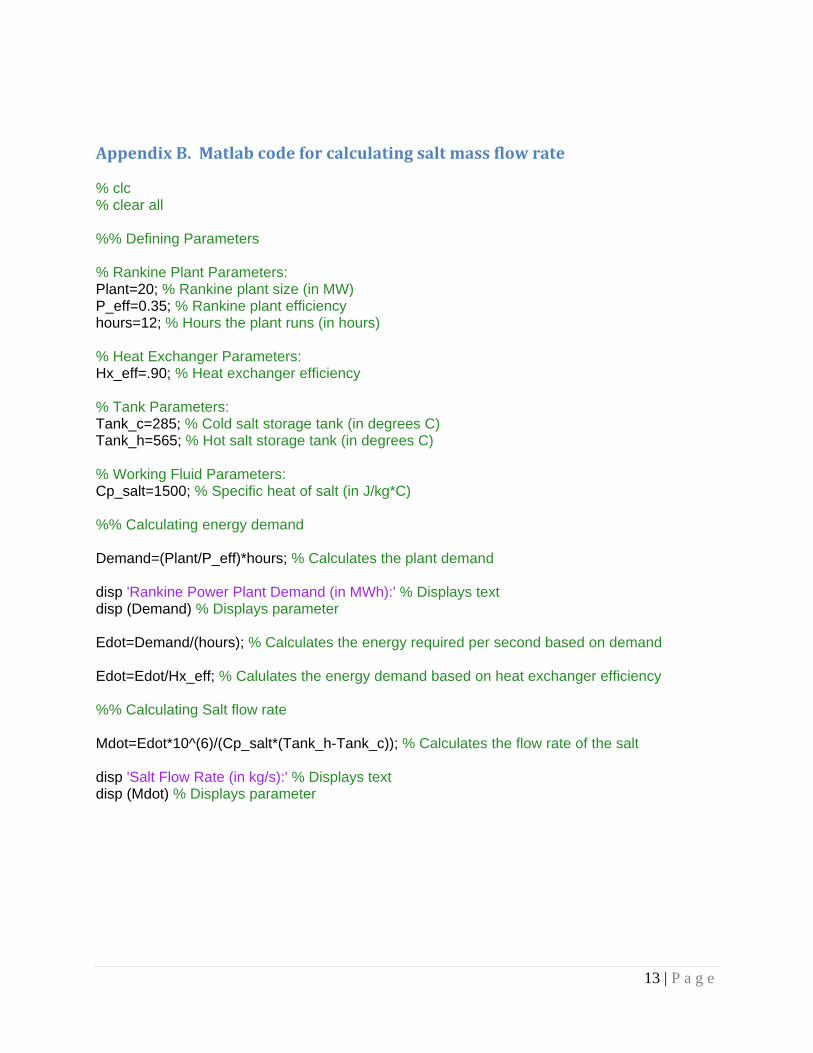
AppendixB.Matlabcodeforcalculatingsaltmassflowrate % clc % clear all %% Defining Parameters % Rankine Plant Parameters: Plant=20; % Rankine plant size (in MW) P_eff=0.35; % Rankine plant efficiency hours=12; % Hours the plant runs (in hours) % Heat Exchanger Parameters: Hx_eff=.90; % Heat exchanger efficiency % Tank Parameters: Tank_c=285; % Cold salt storage tank (in degrees C) Tank_h=565; % Hot salt storage tank (in degrees C) % Working Fluid Parameters: Cp_salt=1500; % Specific heat of salt (in J/kg*C) %% Calculating energy demand Demand=(Plant/P_eff)*hours; % Calculates the plant demand disp 'Rankine Power Plant Demand (in MWh):' % Displays text disp (Demand) % Displays parameter Edot=Demand/(hours); % Calculates the energy required per second based on demand Edot=Edot/Hx_eff; % Calulates the energy demand based on heat exchanger efficiency %% Calculating Salt flow rate Mdot=Edot*10^(6)/(Cp_salt*(Tank_h-Tank_c)); % Calculates the flow rate of the salt disp 'Salt Flow Rate (in kg/s):' % Displays text disp (Mdot) % Displays parameter
Figure 11. Process Flow Diagram (PFD) showing temperatures and mass flow rates.
15 | P a g e
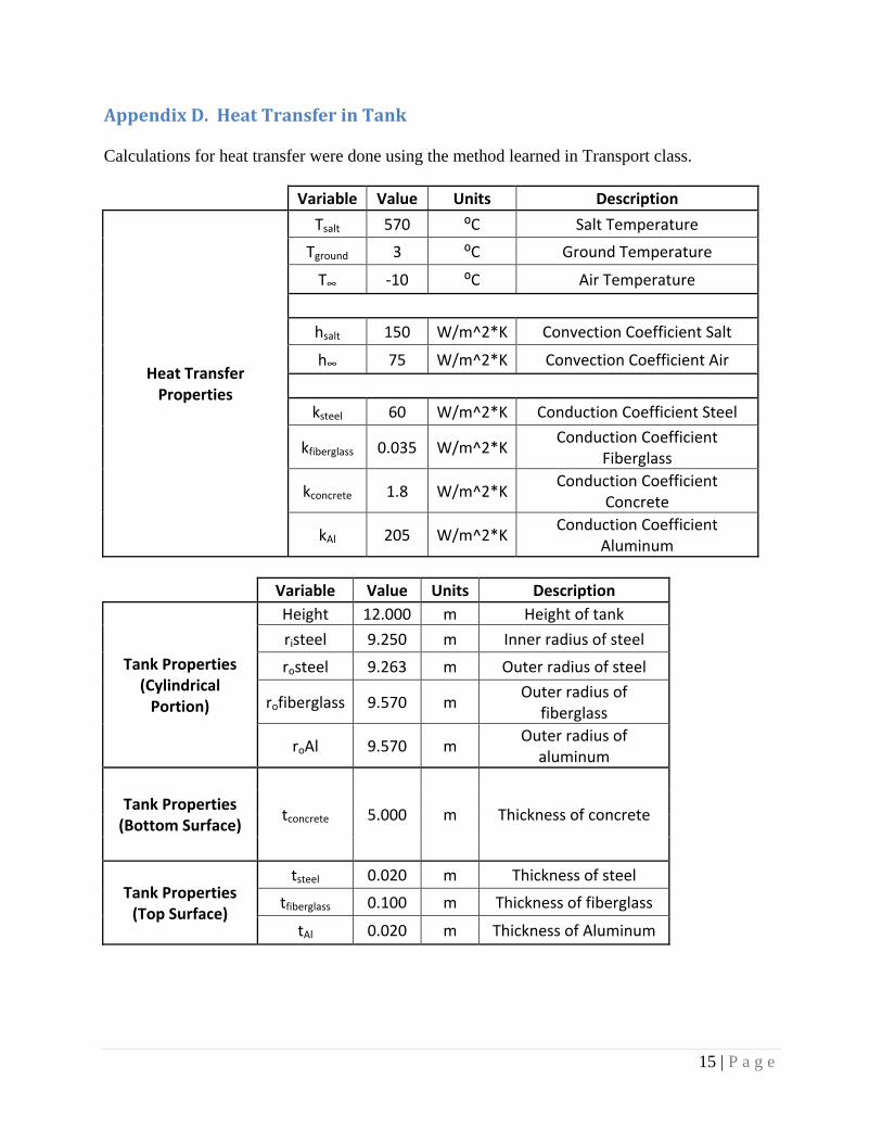
AppendixD.HeatTransferinTank Calculations for heat transfer were done using the method learned in Transport class.
Variable Value Units Description
Heat Transfer Properties
Tsalt 570 ⁰C Salt Temperature
Tground 3 ⁰C Ground Temperature
T∞ ‐10 ⁰C Air Temperature
hsalt 150 W/m^2*K Convection Coefficient Salt
h∞ 75 W/m^2*K Convection Coefficient Air
ksteel 60 W/m^2*K Conduction Coefficient Steel
kfiberglass 0.035 W/m^2*KConduction Coefficient
Fiberglass
kconcrete 1.8 W/m^2*KConduction Coefficient
Concrete
kAl 205 W/m^2*KConduction Coefficient
Aluminum
Variable Value Units Description
Tank Properties (Cylindrical Portion)
Height 12.000 m Height of tank
risteel 9.250 m Inner radius of steel
rosteel 9.263 m Outer radius of steel
rofiberglass 9.570 m Outer radius of
fiberglass
roAl 9.570 m Outer radius of
aluminum
Tank Properties (Bottom Surface)
tconcrete 5.000 m Thickness of concrete
Tank Properties (Top Surface)
tsteel 0.020 m Thickness of steel
tfiberglass 0.100 m Thickness of fiberglass
tAl 0.020 m Thickness of Aluminum
16 | P a g e
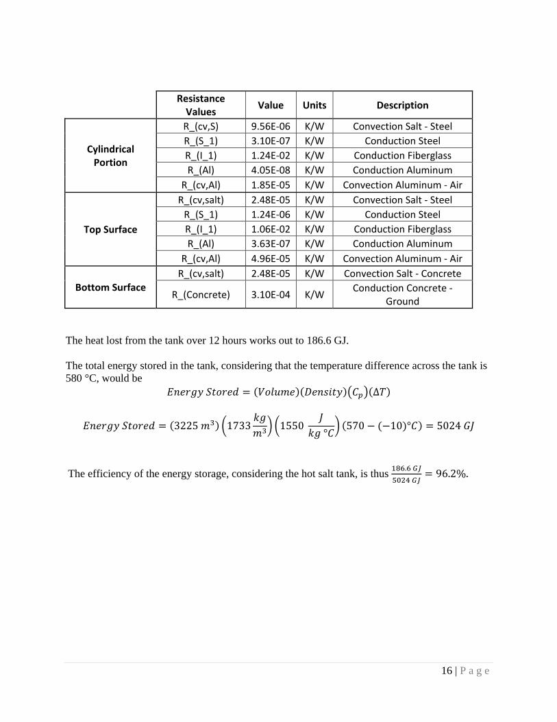
Resistance Values
Value Units Description
Cylindrical Portion
R_(cv,S) 9.56E‐06 K/W Convection Salt ‐ Steel
R_(S_1) 3.10E‐07 K/W Conduction Steel
R_(I_1) 1.24E‐02 K/W Conduction Fiberglass
R_(Al) 4.05E‐08 K/W Conduction Aluminum
R_(cv,Al) 1.85E‐05 K/W Convection Aluminum ‐ Air
Top Surface
R_(cv,salt) 2.48E‐05 K/W Convection Salt ‐ Steel
R_(S_1) 1.24E‐06 K/W Conduction Steel
R_(I_1) 1.06E‐02 K/W Conduction Fiberglass
R_(Al) 3.63E‐07 K/W Conduction Aluminum
R_(cv,Al) 4.96E‐05 K/W Convection Aluminum ‐ Air
Bottom Surface
R_(cv,salt) 2.48E‐05 K/W Convection Salt ‐ Concrete
R_(Concrete) 3.10E‐04 K/W Conduction Concrete ‐
Ground
The heat lost from the tank over 12 hours works out to 186.6 GJ. The total energy stored in the tank, considering that the temperature difference across the tank is 580 °C, would be
∆
3225 1733 1550°
570 10 ° 5024
The efficiency of the energy storage, considering the hot salt tank, is thus .
96.2%.
17 | P a g e
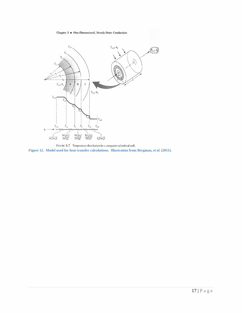
Figure 12. Model used for heat transfer calculations. Illustration from Bergman, et al. (2011).
18 | P a g e
AppendixD.RelativeMaterialsPricingSheet
19 | P a g e
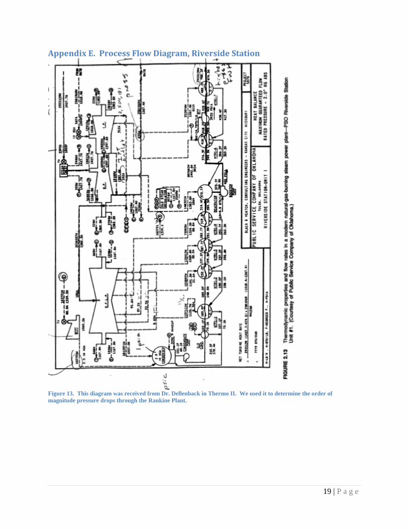
AppendixE.ProcessFlowDiagram,RiversideStation
Figure 13. This diagram was received from Dr. Dellenback in Thermo II. We used it to determine the order of magnitude pressure drops through the Rankine Plant.