68
Bond Graph Modelling of Engineering Systems

Bond Graph Modelling of Engineering Systems

Wolfgang BorutzkyEditor
Bond Graph Modellingof Engineering Systems
Theory, Applications and Software Support
Foreword by Donald Margolis
123

EditorWolfgang BorutzkyBonn-Rhein-Sieg University
of Applied SciencesSankt [email protected]
ISBN 978-1-4419-9367-0 e-ISBN 978-1-4419-9368-7DOI 10.1007/978-1-4419-9368-7Springer New York Dordrecht Heidelberg London
Library of Congress Control Number: 2011927919
c© Springer Science+Business Media, LLC 2011All rights reserved. This work may not be translated or copied in whole or in part without the writtenpermission of the publisher (Springer Science+Business Media, LLC, 233 Spring Street, New York,NY 10013, USA), except for brief excerpts in connection with reviews or scholarly analysis. Use inconnection with any form of information storage and retrieval, electronic adaptation, computersoftware, or by similar or dissimilar methodology now known or hereafter developed is forbidden.The use in this publication of trade names, trademarks, service marks, and similar terms, even ifthey are not identified as such, is not to be taken as an expression of opinion as to whether or notthey are subject to proprietary rights.
Printed on acid-free paper
Springer is part of Springer Science+Business Media (www.springer.com)

Foreword
I am extremely pleased to have been asked to write this Foreword to this compilationtext on bond graph modeling. The contributors to this book are all experts in theirfields and I consider all of them to be friends. I have ample evidence from my 40+years of working in the mechatronics area that physical system understanding isimperative for the design of modern engineering systems. It remains essential to beable to represent physical systems in a uniform way such that analytical or computerresponse predictions can be straightforwardly carried out.
Bond graphs are a concise pictorial representation of all types of interactingenergetic systems. In my experience working with engineers on the developmentof complex systems it is obvious that these systems suffer from thermal problems,structural problems, vibration and noise problems, and control and stability issuesthat do not fit into a single discipline. Bond graphs provide the link by which allthese different disciplines can be represented in an overall system model. I am cer-tain that bond graphs are the best way to study and solve these multi-energy domainsystem problems.
Bond graphs were invented by Professor Henry Paynter at M.I.T. We jokinglyassign the bond graph birthday as April 24, 1954. I was fortunate to have Hankas an adviser and I learned a lot from him while trying to keep up with his ideas.Hank was probably a genius but definitely not a detail-oriented person. While Hankwas able to construct bond graph models in his own mind, he did not take the timeto develop the rules by which the rest of us could construct a bond graph model.This was left to his students, Professors Dean Karnopp and Ronald Rosenberg. Theydeveloped the concepts of power convention and the causal stroke and developed thefirst computer program that could interpret a bond graph description and generatea set of state space equations. Now there are many computer programs that can gofrom a bond graph picture to a simulation of a nonlinear system in a straightforward,systematic approach.
Bond graph modeling has come a long way since these early days. There areliterally tens of thousands of publications that use bond graphs. There are courses atuniversities all over the world that teach bond graph modeling in incredibly diverseareas such as chemical physics, biophysics, nanotechnology, and cell dynamics.There was a time when I knew practically every bond grapher in the world. Thattime has long passed as more and more disciplines recognize the value of a unified
v

vi Foreword
approach to modeling all types of physical systems, producing both linear and non-linear mathematical models.
This book is a compilation of contributions from outstanding researchers all overthe world in the field of bond graph modeling and theory. There are introductorytopics for the uninitiated, topics on bond graph theory, and a wealth of informationon applications of bond graphs to realistic mechatronic systems. I hope that thereaders will enjoy this book and find it most useful for their engineering careers.
Davis, California Donald MargolisDecember 2010

Preface
This multi-author book reflects the present state of the art in bond graph modellingof engineering systems with respect to theory, applications and software support.Bond graph modelling is a physical modelling methodology based on first princi-ples that is particularly suited for modelling multidisciplinary or mechatronic sys-tems. Bond graphs were devised by Professor H. Paynter some 50 years ago atthe Massachusetts Institute of Technology (MIT) in Cambridge, MA, USA. As tothe pioneers of this methodology, the authors of this book are indebted to, amongothers, Professor D. Karnopp and Professor D. Margolis (University of Californiaat Davis), Professor R. Rosenberg (Michigan State University, East Lansing, MI),Professor J. Thoma (Professor Emeritus at the University of Waterloo, ON, Canada)and Professor J.J. van Dixhoorn (University of Twente, Enschede, the Netherlands.
Since the early days, bond graph modelling has evolved into a powerful richmethodology. Considerable progress has been achieved since then. Bond graphmodelling has spread all over the world. It is used in engineering education as well asin industrial projects. Numerous bond graph-related papers have been presented ininternational conferences and published in refereed scientific journals. Furthermore,bond graph modelling has been used in many Ph.D. theses and has been the subjectof a number of monographs and textbooks in various languages.
Beyond some special journal issues devoted to bond graph modelling, to theknowledge of the editor, very few multi-author books on bond graph modellinghave been published during the past decades. One book to be mentioned is the1991 compilation text Bond Graphs for Engineers edited by P. Breedveld andG. Dauphin-Tanguy. Another contributed book titled Les bond graphs was editedby G. Dauphin-Tanguy and published in 2000. A survey of bond graph-related pub-lications suggests that it was time for a new collection that covers achievementsand recent developments in bond graph modelling by integrating various works andpresenting them in a uniform manner. On invitation by Springer, the editor of thisbook asked colleagues active in the realm of bond graph modelling for contributions.This book is the outcome of a truly international worldwide successful cooperationof excellent young researchers and those who have been using bond graphs and havebeen teaching the methodology for a long time. The book covers some theoreticalissues and methodology topics that have been the subject of ongoing research duringpast years, presents new promising applications such as the bond graph modelling of
vii

viii Preface
fuel cells and illustrates how bond graph modelling and simulation of mechatronicsystems can be supported by software. This up-to-date comprehensive presentationof various topics has been made possible by the cooperation of a group of authorswho are experts in various fields and share the “bond graph way of thinking”.
The aim of this contributed book is to reflect the current state of the art in bondgraph modelling by presenting and discussing advanced recent topics. However, allchapters have been written in such a way that newcomers to the methodology withsome knowledge of the basics may easily get into the vast fascinating and open fieldof advanced bond graph modelling. Readers who may want to have a closer look atbond graph fundamentals will find references to latest monographs and textbooks.Furthermore, each chapter provides many references to conference papers, journalarticles and Ph.D. theses on advanced topics.
Bond Graph Modelling of Engineering Systems: Theory, Applications and Soft-ware Support addresses readers in academia as well as engineers in industry andinvites experts in related fields to consider the potential and the state of the art ofbond graph modelling. This multi-author book well complements latest monographsand textbooks on bond graph modelling and may serve as a guide for further self-study and as a reference.
Sankt Augustin, Germany Wolfgang BorutzkyDecember 2010

Acknowledgements
This book would not have been possible without the commitment of my colleagues.I would like to take this opportunity to thank all my co-authors for their con-tributed chapters. Likewise, I wish to thank all colleagues who took the time tocarefully review the chapters. Their valuable comments and suggestions are grate-fully acknowledged.
Also, I appreciate the support this multi-author book project receivedfrom Professors Yuri Merkuryev, Riga Technical University, Latvia; DavidMurray-Smith, University of Glasgow, Scotland, UK; Ronald Rosenberg, MichiganState University, East Lansing, MI, USA; and Jean Thoma, University of Waterloo,ON, Canada.
Last but not least, I wish to thank my editor with Springer at New York, NY, USA,Brett Kurzman, for his invitation to this book project, for allowing us to exceed theinitially envisaged page limit and for his constant support during this book project.
Sankt Augustin, Germany Wolfgang BorutzkyDecember 2010
ix


Contents
Part I Bond Graph Theory and Methodology
1 Concept-Oriented Modeling of Dynamic Behavior . . . . . . . . . . . . . . . . 3P.C. Breedveld
2 Energy-Based Bond Graph Model Reduction . . . . . . . . . . . . . . . . . . . . . 53L.S. Louca, D.G. Rideout, T. Ersal, and J.L. Stein
3 LFT Bond Graph Model-Based Robust Fault Detectionand Isolation . . . . . . . . . . . . . . . . . . . . . . . . . . . . . . . . . . . . . . . . . . . . . . . . . . 105M.A. Djeziri, B. Ould Bouamama, G. Dauphin-Tanguy,and R. Merzouki
4 Incremental Bond Graphs . . . . . . . . . . . . . . . . . . . . . . . . . . . . . . . . . . . . . 135Wolfgang Borutzky
Part II Bond Graph Modelling for Design, Control, and Diagnosis
5 Coaxially Coupled Inverted Pendula: Bond Graph-BasedModelling, Design and Control . . . . . . . . . . . . . . . . . . . . . . . . . . . . . . . . . 179P.J. Gawthrop and F. Rizwi
6 Bond Graphs and Inverse Modeling for Mechatronic System Design 195Wilfrid Marquis-Favre and Audrey Jardin
7 Bond Graph Model-Based Fault Diagnosis . . . . . . . . . . . . . . . . . . . . . . . 227S.K. Ghoshal and A.K. Samantaray
Part III Applications
8 Bond Graph Modeling and Simulation of Electrical Machines . . . . . . 269Sergio Junco and Alejandro Donaire
9 Simulation of Multi-body Systems Using Multi-bond Graphs . . . . . . . 323Jesus Felez, Gregorio Romero, Joaquín Maroto, and María L. Martinez
xi

xii Contents
10 Bond Graph Modelling of a Solid Oxide Fuel Cell . . . . . . . . . . . . . . . . . 355P. Vijay, A.K. Samantaray, and A. Mukherjee
Part IV Software for Bond Graph Modelling and Simulation
11 Automating the Process for Modeling and Simulationof Mechatronics Systems . . . . . . . . . . . . . . . . . . . . . . . . . . . . . . . . . . . . . . . 385Jose J. Granda
Index . . . . . . . . . . . . . . . . . . . . . . . . . . . . . . . . . . . . . . . . . . . . . . . . . . . . . . . . . . . . 431

Contributors
Wolfgang Borutzky Bonn-Rhein-Sieg University of Applied Sciences, SanktAugustin, Germany, [email protected]
P.C. Breedveld University of Twente, EWI/EL/CE, AE Enschede,The Netherlands, [email protected]
G. Dauphin-Tanguy LAGIS FRE CNRS, Villeneuve d’Ascq Cedex, France,[email protected]
M.A. Djeziri LAGIS FRE CNRS, Villeneuve d’Ascq Cedex, France,[email protected]
Alejandro Donaire Centre for Complex Dynamic Systems and Control (CDSC),The University of Newcastle, Callaghan, NSW, Australia; Laboratorio deAutomatización y Control, Departamento de Control, Facultad de Ciencias Exactas,Ingeniería y Agrimensura, FCEIA, Universidad Nacional de Rosario, Ríobamba245 bis, S2000EKE, Rosario, Argentina, [email protected]
T. Ersal Department of Mechanical Engineering, University of Michigan, AnnArbor, MI, USA, [email protected]
Jesus Felez CITEF, Universidad Politécnica de Madrid (UMP), Madrid, Spain;ETSI Industriales, Universidad Politécnica de Madrid (UMP), Madrid, Spain,[email protected]
P.J. Gawthrop School of Engineering, University of Glasgow, Scotland, UK,[email protected]
S.K. Ghoshal Department of Mechanical Engineering and Mining MachineryEngineering, Indian School of Mines, Dhanbad, India,[email protected]
Jose J. Granda Department of Mechanical Engineering, California StateUniversity, Sacramento, CA, USA; Institute for Dynamic Systems andControl ETH, Swiss Federal Institute of Technology, Zurich, Switzerland,[email protected]
xiii

xiv Contributors
Audrey Jardin Laboratory Ampère, Institut National des Sciences Appliquées deLyon (INSA), University of Lyon, Villeurbanne Cedex, France,[email protected]
Sergio Junco Laboratorio de Automatización y Control, Departamento de Control,Facultad de Ciencias Exactas, Ingeniería y Agrimensura, FCEIA, UniversidadNacional de Rosario, Ríobamba 245 bis, S2000EKE, Rosario, Argentina,[email protected]
L.S. Louca Department of Mechanical and Manufacturing Engineering, Universityof Cyprus, Nicosia, Cyprus, [email protected]
Joaquín Maroto CITEF, Universidad Politécnica de Madrid (UMP), Madrid,Spain; ETSI Industriales, Universidad Politécnica de Madrid (UMP), Madrid,Spain, [email protected]
Wilfrid Marquis-Favre Laboratory Ampère, Institut National des SciencesAppliquées de Lyon (INSA), University of Lyon, Villeurbanne Cedex, France,[email protected]
María L. Martinez CITEF, Universidad Politécnica de Madrid (UMP), Madrid,Spain; ETSI Industriales, Universidad Politécnica de Madrid (UMP), Madrid,Spain, [email protected]
R. Merzouki LAGIS FRE CNRS, Villeneuve d’Ascq Cedex, France,[email protected]
A. Mukherjee Department of Mechanical Engineering, Indian Instituteof Technology, Kharagpur, India, [email protected]
B. Ould Bouamama LAGIS FRE CNRS, Villeneuve d’Ascq Cedex, France,[email protected]
D.G. Rideout Faculty of Engineering and Applied Science, Memorial University,St. John’s, NL, Canada, [email protected]
F. Rizwi Commonwealth Scientific and Industrial Research Organisation (CSIRO),Hobart, Tasmania, Australia, [email protected]
Gregorio Romero CITEF, Universidad Politécnica de Madrid (UMP), Madrid,Spain; ETSI Industriales, Universidad Politécnica de Madrid (UMP), Madrid,Spain, [email protected]
A.K. Samantaray Department of Mechanical Engineering, Indian Instituteof Technology, Kharagpur, India, [email protected]
J.L. Stein Department of Mechanical Engineering, University of Michigan,Ann Arbor, MI, USA, [email protected]
P. Vijay Department of Chemical Engineering, Curtin University of Technology,Perth, WA, Australia, [email protected]

Abbreviations
2D two-dimensional3D three-dimensionalAC alternating currentAR axis rotatorARR analytical redundancy relationBDF backward differentiation formulaBG bond graphBLDCM brushless direct current motorCAI cumulative activity indexCCIP coaxially coupled inverted pendulacemf counter-electromotive forceDAE differential-algebraic equationDBG diagnostic bond graphDC direct currentDCM direct current motor/machineDFIM doubly fed induction machineDHBG diagnostic hybrid bond graphDI detectability indexDOF degree of freedomECI energetic contribution indexEJS Eulerian junction structureemf electromotive forceFDI fault detection and isolationFSM fault signature matrixFU fuel utilizationGARR generalized ARRGYS gyristorHBG hybrid bond graphHMMWV high-mobility multipurpose wheeled vehicleIM induction motor/machineIncBG incremental bond graphKLE Karhunen–Loève expansionLFT linear fractional transformation form
xv

xvi Abbreviations
LPV linear parameter-varyingLTI linear time-invariant systemMBG multibond graphMBS multibody systemMEA membrane electrode assemblyMGY modulated gyratorMIMO multiple input–multiple output systemmmf magnetomotive forceMODA model order deduction algorithmMORA model order reduction algorithmMTF modulated transformerODE ordinary differential equationOU oxygen utilizationPI proportional plus integral (controller)PM permanent magnetPMDCM permanent magnet direct current motor/machinePMSM permanent magnet synchronous motorPWM pulse width modulationRA relative activityRHP right half planeRMS root mean squareSCAP sequential causality assignment procedureSISO single input–single output systemSOFC solid oxide fuel cellSPJ switched power junctionSRM switched reluctance motorTCG temporal causal graphTPB triple phase boundaryUIO unknown input observerVSI voltage source inverterZC zero complianceZCP zero-order causal path

Part IBond Graph Theory and Methodology
Part I of this book addresses theoretic foundations and concepts of bond graphmodelling. Moreover, it presents methodologies for a bond graph-based solutionof various types of problems.
Chapter 1 closely reviews the model development process. After a formal foun-dation of bond graphs, principles and fundamental concepts of port-based physicalsystems modelling in terms of bond graphs are pointed out and are discussed in aclarifying way that may help avoid model developers to fall into traps, to overlookassumptions and the context dependency of models, or to mix concepts which maygive rise to confusions, e.g. with regard to ideal concepts and physical components.A key issue of Chapter 1 is that it emphasises the distinction between configurationstructure, physical structure, and conceptual structure.
Clearly, a model to be developed should meet the accuracy requirements ofan application and at the same time should be as simple as possible. However,as today’s engineering systems tend to become larger, more complex, and moreintegrated, it is not always obvious at the beginning of a modelling process whichphenomena are relevant with regard to the application and to decide what to includeinto a model and what to neglect. As a result, one approach often applied is tostart with a complex model and to reduce its complexity subsequently as far as theapplication permits.
Chapter 2 presents three model reduction techniques based on the considerationof energy flows in a bond graph model. One approach ranks energy stores and dis-sipators on the basis of a power norm called activity in order to reduce the modelcomplexity by eliminating the least ‘active’ elements.
Chapter 3 introduces a special decomposition of bond graph elements in a partwith nominal parameters and one with uncertain parameters. The resulting bondgraph model of a bond graph element is called linear fractional transformation (LFT)model. In case of linear models, bond graphs with elements replaced by their LFTmodel enable the derivation of state space and output equations in LFT form as usedfor stability analysis and control law synthesis based on μ-analysis.
Moreover, LFT bond graphs can also support robust fault detection and isolation(FDI) of systems with uncertain parameters. The decomposition of bond graph ele-ments leads to a derivation of analytical redundancy relations (ARRs) composed ofa nominal part representing their residuals and an uncertain part due to parameter

2 Part I Bond Graph Theory and Methodology
uncertainties. The latter one can be used for the calculation of adaptive thresholdsand for a parameter sensitivity analysis of the residuals.
Incremental bond graphs present another approach. Similar to the LFT bondgraph approach, they are obtained by replacing elements by their incremental model.The latter one is also a decomposition of a bond graph element into a nominal partand one that accounts for parameter variations. Opposed to LFT bond graphs, bondsof incremental bond graphs carry variations of the conjugated power variables dueto parameter variations.
Chapter 4 shows how incremental bond graphs enable a matrix-based determina-tion of parameter sensitivities of transfer functions for direct as well as for inverselinear models. The necessary matrices can be generated from a bond graph and itsincremental bond graph by means of existing software. Furthermore, incrementalbond graphs also support a parameter sensitivity analysis of ARR residuals.

Chapter 1Concept-Oriented Modelingof Dynamic Behavior
P.C. Breedveld
Abstract This chapter introduces the reader to the concept-oriented approach tomodeling that clearly separates ideal concepts from the physical components of asystem when modeling its dynamic behavior for a specific problem context. Thisis done from a port-based point of view for which the domain-independent bondgraph notation is used, which has been misinterpreted over and over, due to theparadigm shift that concept-oriented modeling in terms of ports requires. For thatreason, the grammar and semantics of the graphical language of bond graphs arefirst defined without making any connection to the physical modeling conceptsit is used for. In order to get a first impression of how bond graphs can repre-sent models, an existing model is transformed into bond graphs as the transfor-mation steps also give a good impression of how this notation provides immediatefeedback on modeling decisions during actual modeling. Next, physical systemsmodeling in terms of bond graphs is discussed as well as the importance of therole of energy and power that is built into the semantics and grammar of bondgraphs. It is emphasized that, just like circuit diagrams, bond graphs are a topo-logical representation of the conceptual structure and should not be confused withspatial structure. By means of a discussion of some examples of such confusionsit is explained why bond graphs have a slow acceptance rate in some scientificcommunities.
Keywords Labeled di-graph · Node categorization · Energy and co-energy ·Legendre transform · Thermodynamic framework of variables · Generalizedmechanic framework of variables · Equilibrium-determining variable · Equilibrium-establishing variable
P.C. Breedveld (B)University of Twente, EWI/EL/CE, 7500 AE Enschede, The Netherlandse-mail: [email protected]
W. Borutzky (ed.), Bond Graph Modelling of Engineering Systems,DOI 10.1007/978-1-4419-9368-7_1, C© Springer Science+Business Media, LLC 2011
3

4 P.C. Breedveld
1.1 Introduction
Many models are constructed to obtain better insight into the dynamic behaviorof all sorts of real-world systems and processes, however, often without carefulconsideration of what the meaning of such a model is. This is due to the fact that itis easy to fall into the trap of (unconsciously) extrapolating the meaning of a modelto interpretations that violate the original assumptions that led to the abstraction athand. Apart from the aim to introduce the port-based approach in terms of bondgraphs in this book, this contribution is written with the aim to make clear thata model is such an abstraction that focuses on particular aspects of a part of thereal world, given a problem with the real world or question about it, even if it is aquestion about some future realization (design). In all cases, this makes the modelhighly dependent on the context of that problem, even when the question is quitegeneral: the person(s) making the abstraction will always do so from a particularviewpoint and background. As a result, models are often highly dependent on (sci-entific) culture and its jargon, even when this culture is mathematics or rather math-ematical physics, which has the longest tradition in carefully using unambiguousconcepts.
Herein, we will try to carefully step through the process of creating a dynamicmodel of a system or process that is assumed to obey the principles of classicalphysics (to be enumerated later). During this journey we will point out why andhow things can go wrong the way they often do. In the introduction of the catalogueof an exposition created by Wim Beeren called ‘Traces of Science in Art’ nuclearphysicist Walter H. G. Lewin searches for the reason why art and science have somany parallels. “Both try,” he writes, “to expose new ideas; they seek essence andclarity. The goal is a new opinion, a new way of looking at things which we are notused to. Never, therefore, the familiar – and so confirmational – comfort of a ‘warmbed’, but always the uncomfortable but potentially very revealing ‘cold floor’” [1].
During the following journey through the conceptual world of dynamic behavior,some readers, including Walter Lewin when he would read this, may also feel thiscold floor, in particular when we discuss one of Lewin’s lectures that are avail-able on YouTube (Part 1: http://www.youtube.com/watch?v=eqjl-qRy71w, Part 2:http://www.youtube.com/watch?v=1bUWcy8HwpM) as an example of how ignor-ing implicit assumptions of a modeling technique may lead to misleading paradoxes.The reader is advised to watch the lectures beforehand and is challenged to answerthe question of who was cheating, Lewin or his colleagues in the audience . . .
In order to be able to represent the models and modeling issues that will bediscussed in an insightful way, the abstractions will not only be expressed in terms ofmathematical equations, but primarily in a graphical notation for port-based modelscalled bond graphs [2]. As many negative prejudices exist about this notation andits use, most of them unjustified [3], we will start by simply defining the notationitself that has a graph-theoretic foundation, while keeping it free from any (physical)interpretation for the time being, even when the terminology seems to induce suchan interpretation. At a later stage this notation will be used to explain a specificphysical interpretation of models known as the port-based approach to modeling.

1 Concept-Oriented Modeling of Dynamic Behavior 5
1.2 Graph-Theoretic Foundation of Bond Graphs
1.2.1 Introduction
An often heard argument to reject the ideas represented by bond graphs is that theyare not well defined, at least mathematically speaking. Therefore, a unique definitionof this graphical language will be given first, while being aware of the fact that eachlanguage has its dialects, just like any other mathematical paper that needs a properlist of symbols and a set of definitions too. The existence of a dialect does not meanthat the meaning becomes ambiguous: for each case unambiguous definitions shouldalways be possible and preferably made explicit along the same lines as the ones tofollow.
1.2.2 Bond Graphs
A bond graph is a labeled di-graph – directed graph, i.e., ‘a graph in which each linkhas an assigned orientation’ [4] – of which the two types of edges are called bondsand signals and the labeled nodes are called multiport nodes or, if no confusion ispossible, just multiports, where the number of bonds connected to a node corre-sponds to the number of ports of a multiport, including the concept of a one-port.Each signal connected to a node with inward orientation is said to modulate themultiport, which in turn is called a modulated multiport, unless no bonds but onlysignals are connected to the node, in which case the signal is just an input of a so-called block diagram-type node. A block diagram is a computational diagram thatonly contains signal edges and (functional) block nodes that represent an operatoron the input(s). A signal is connected to a signal port. It may depend on the contextif the concept of the number of ports in a description of a multiport refers to the totalnumber of ports, including or excluding the signal ports, but the description shouldmake this clear. In case of doubt a clear distinction should be made between portsfor signals and ports for bonds. Bonds are represented by augmenting the edge withits direction in the graph by means of a small line that turns the representation ofthe edge into a half arrow and signals are represented by augmenting the edge withits direction by means of an arrow head, usually two small lines that turn it into afull arrow (Fig. 1.1). The labels can consist of contoured descriptions (word bond
Fig. 1.1 Labeled di-graphwith bonds and signals
Type1
Type1
Type2
Block1
Type3
:Node1
Node2:
:Node3
:Signal node
:Node4

6 P.C. Breedveld
graph), mnemonic codes consisting of a limited number of alphanumeric symbols,or graphical symbols (in case block diagram symbols represent operations on sig-nals). The node label indicates the type of the node. If a particular instantiation of anode type needs to be specified, this is done by means of a colon and a specific name.For linear one-ports this name commonly consists of its constitutive parameter.
Multiple edges of the same type between two nodes may be represented in acombined manner by using condensed edge symbols consisting of two (or more,in case of underlying hierarchy) parallel edges (lines), if necessary with a number(or array of numbers) indicating its dimension(s), i.e., the number(s) of bonds orsignals that form this so-called multibond (array) or multisignal (array), respectively.Collections of nodes may be condensed into (a hierarchy of) arrays by underlining.This multibond notation has been defined before [5, 6] and will not be discussed indetail herein as it would distract from the main message and is only meant to allowzooming in order to keep large graphs manageable and insightful.
1.2.3 Ports and Bonds
Each port of a multiport, i.e., the interface between a bond and a multiport node,is characterized by two real variables of time that are called effort (e) and flow ( f )and that are considered ‘dynamically conjugated.’ They are scalars in case of singlebond edges and vectors in the sense of one-column matrices in case of multibondedges. If their (inner) product is called a power (P) these variables are called powerconjugated, the bond is called a power bond, and the port to which it is connectedis a power port, without linking it to some physical interpretation yet. Bond graphsthat only contain power bonds and signals are sometimes called true bond graphsas opposed to the larger class of pseudo-bond graphs in which the efforts and flowsare considered to be only dynamically conjugated (terminology to be explained inmore detail in Section 1.5.6). The nodes in a true bond graph have true power portsand are connected by true bonds. When it is obvious that no confusion can arise truebond graphs are just called bond graphs and power bonds just bonds. Even thoughthis terminology already suggests some relation with modeling of physical systembehavior, this interpretation is deliberately postponed until the discussion of port-based modeling itself. This means that the property of variables being ‘conjugated’just expresses at this time that they belong to the same port.
The attachment of a signal to a node is called a signal port. There are two typesof signal ports: inputs and outputs. A signal interconnects an output to an input.The full arrow of the signal is attached to an input and its open end to an output.This interconnection has a unique meaning: connecting two signal ports by a signalequates the variables on each signal port to those on the signal and thus to each other(Fig. 1.2). This means that the dimensions and units of the variables that are equatedby a signal should correspond to each other.
The multiport itself relates all efforts and flows at its ports fundamentally in sucha way that each power port has a dependent and an independent (effort or flow)

1 Concept-Oriented Modeling of Dynamic Behavior 7
s1 s2
s = s1 = s2Node1: Type 1 Type 2 :Node2
Fig. 1.2 Signal connecting two signal ports in a graph fragment
variable. These relations are called constitutive relations and may also depend onthe input signals of the multiport (independent variables of the multiport). Outputsignals may depend on any of the independent variables of a multiport. In somecases where the desired dynamic behavior of both conjugate variables is taken asa starting point, the constitutive relation itself (constitutive parameter in the linearcase) is chosen to be the unknown, such that the fundamental shape of the aboverelation is violated. However, this does not correspond to a dynamic model anymore,but to the use of a dynamic model structure for changing its dynamic properties ina design context. We will address this anomaly later, as there is a branch of theliterature that uses bond graphs for this purpose.
A (multi)bond equates the efforts of the connected ports to each other. Similarlyit equates the flows of the ports it connects to each other. As a result, the effortand flow variables can also be considered to live on the (multi)bond (Fig. 1.3). Thismeans that the property of variables being ‘conjugated’ also expresses that theybelong to the same bond and that the dimensions of the variables that are equatedby a (multi)bond should correspond to each other.
e2
f2
e = e1 = e2
f = f1 = f2
e1f1
Node1: Type 1 Type 2 :Node2
Fig. 1.3 Signal connecting two signal ports in a graph fragment
1.2.4 Causal Stroke
From the fact that one of the variables on a port is an independent variable of theconstitutive relation and the other one a dependent variable, it follows that the com-putational direction of the two conjugate variables at a bond is always bi-directionaland can in principle be expanded into two opposite signals, in other words, a bondcan be considered a bilateral signal flow. The effort is the input of the multiport nodeat the one side and the output of the node at the other side. Only after a particularchoice is made about the two possibilities of these directions, this can be representedby ‘causally augmenting’ the (multi)bond with a so-called causal stroke, a little linedrawn orthogonal to the bond at the end of the bond where the effort serves asan output of the bond from a computational point of view. This implicates that itserves as an input for the port that is connected to that side of the bond. Similarlythe conjugate flow at that side of the bond is an output of this port and an input to

8 P.C. Breedveld
e e
ff f
Type 1
Type 1
Type 1
Type 1
Type 2
Type 2
Type 2
Type 2
Fig. 1.4 Meaning of the causal stroke: direction of the bilateral signals
the bond. Obviously, the open end of the bond at the other side reverses this storyfor the port connected to the other side of the bond: effort is output of port andinput of bond and flow is input of port and output of bond (Fig. 1.4). The featureof a bond that it can also be drawn without a causal stroke, i.e., without fixing thecomputational directions of the bilateral signal flow, is one of the main advantages ofa port-based approach during modeling and in particular for the re-use of submodels,as it expresses that the causal form of the constitutive relations should not be fixeda priori and left open where possible in order to facilitate interconnection.
A signal represents one arbitrary variable of time that may also be an effort ora flow, but not necessarily. Its computational direction is fixed by definition andrepresented by a full arrow which clearly distinguishes it from the bilateral signalflow represented by a (power) bond. In the particular case that a signal represents aneffort or flow, it can be considered a so-called activated bond, i.e., a bond of whichthe conjugate variable is negligible and thus considered zero-valued, consequentlynot playing a role at the side of the edge where there is no arrow and resulting in theinner product of the conjugate variables being zero. As discussed in more detail inSection 1.3 this can be considered as the representation of the concept of an idealsensor.
Only ports with the same types of efforts and flows can be connected to eachother by a bond. A particular type of effort and flow belongs to a domain. Table 1.1shows a list of domains and the corresponding names of the effort and flow typesthat belong to that domain. Again we emphasize that, even though the terminologyin this table suggests a strong connection with physical system modeling, this con-nection is postponed until the discussion of physical system modeling itself. In otherwords, Table 1.1 just defines the terminology and the interconnection constraints, asonly ports that belong to the same domain can be connected by a bond. However,as this table is based on a thermodynamic framework of variables (to be discussedin Section 1.5.6) it may be unfamiliar to many readers who have a background inanalog system modeling that is commonly using the mechanical framework of vari-ables (Table 1.2) in which some domains are combined to one domain by addinga different kind of state (generalized momentum) [7]. This will be discussed inSection 1.5.

1 Concept-Oriented Modeling of Dynamic Behavior 9
Table 1.1 Thermodynamic framework of domains and variables
fflowEquilibriumestablishing
eeffortEquilibrium determining,intensive state
q = ∫f dt
Generalized state,extensive state
Electric iCurrent
uVoltage
q = ∫i dt
Charge
Magnetic uVoltage
iCurrent
λ = ∫u dt
Magnetic flux linkage
Elastic/potentialtranslation
v
VelocityFForce
x = ∫v dt
Displacement
Kinetictranslation
FForce
v
Velocityp = ∫
F dtMomentum
Elastic/potentialrotation
ω
Angular velocityTTorque
θ = ∫ω dt
Angular displacement
Kinetic rotation TTorque
ω
Angular velocityb = ∫
T dtAngular momentum
Elastic hydraulic ϕ
Volume flowpPressure
V = ∫ϕ dt
Volume
Kinetic hydraulic pPressure
ϕ
Volume flowΓ = ∫
p dtMomentum of a flow tube
Thermal TTemperature
f SEntropy flow
S = ∫fS dt
Entropy
Chemical μ
Chemicalpotential
f NMolar flow
N = ∫fN dt
Number of moles
An arbitrary node of a bond graph is a multiport, i.e., a node with multiple(power) ports and it may also have signal ports. This multiport can be categorizedbased on the nature of the relations between the involved (power) port variables andsignals. An arbitrary node may be represented in a bond graph by a short descrip-tion (label) enclosed by an ellipse, resulting in a so-called word bond graph [8].The only generic properties of this multiport are that it represents the constitutiverelations between a number of efforts and a number of flows that are both equalto the number of (power) ports and thus equal itself and that each port has oneindependent and one dependent variable (either the effort or the flow) in the relationand between a number of arbitrary variables that is equal to the number of inputsignal ports. Output signal ports result in additional constitutive relations that relatethe output to one or more independent variables. For a multiport with n ports, k inde-pendent flows f , n − k independent efforts e, r outputs u, and s inputs i this can bewritten as

10 P.C. Breedveld
Table 1.2 Conventional domains with corresponding flow, effort, generalized displacement, andgeneralized momentum
fflow
eeffort
q = ∫f dt
Generalizeddisplacement
p = ∫e dt
Generalizedmomentum
Electromagnetic iCurrent
uVoltage
q = ∫i dt
Chargeλ = ∫
u dtMagnetic flux
linkage
Mechanicaltranslation
v
VelocityFForce
x = ∫v dt
Displacementp = ∫
F dtMomentum
Mechanicalrotation
ω
Angular velocityTTorque
θ = ∫ω dt
Angulardisplacement
b = ∫T dt
Angularmomentum
Hydraulic/pneumatic
ϕ
Volume flowpPressure
V = ∫ϕ dt
VolumeΓ = ∫
p dtMomentum of a
flow tube
Thermal TTemperature
f SEntropy flow
S = ∫fS dt
Entropy
Chemical μ
Chemicalpotential
f NMolar flow
N = ∫fN dt
Number ofmoles
⎡
⎢⎢⎢⎢⎢⎢⎢⎢⎢⎢⎢⎢⎢⎢⎢⎣
e1...
ek
fk+1...
fn
u1...
ur
⎤
⎥⎥⎥⎥⎥⎥⎥⎥⎥⎥⎥⎥⎥⎥⎥⎦
=
⎡
⎢⎢⎢⎢⎢⎢⎢⎢⎢⎢⎢⎢⎢⎢⎢⎣
e1 (x)...
ek (x)fk+1 (x)...
fn (x)u1 (x)...
ur (x)
⎤
⎥⎥⎥⎥⎥⎥⎥⎥⎥⎥⎥⎥⎥⎥⎥⎦
with x =
⎡
⎢⎢⎢⎢⎢⎢⎢⎢⎢⎢⎢⎢⎢⎢⎢⎣
f1...
fk
ek+1...
en
i1...
is
⎤
⎥⎥⎥⎥⎥⎥⎥⎥⎥⎥⎥⎥⎥⎥⎥⎦
(1.1)
A categorization of these constitutive relations allows further categorization ofthe nodes and simpler and more generic labeling. While still making no relation toport-based modeling, these categories will be quite general and when the connectionto port-based modeling is made further restrictions can be made, highly depend-ing on the modeling level though, as will be explained when discussing modelingitself. All categories allow the presence of an arbitrary number of outputs (meaningnothing else than making a variable available as independent variable at an inputof another multiport). An arbitrary number of inputs is also allowed: this has beenintroduced already as ‘modulation’ (modulated multiport) and each signal is a mod-ulation signal or modulating signal. Note that one can also consider a multiport asbeing a node with an arbitrary number of inputs and an arbitrary number of outputs
1 Concept-Oriented Modeling of Dynamic Behavior 11
of which a number (n) of inputs are conjugated (paired) to n outputs while leavingthe question open which of the variables in a pair gets the role of input or output aslong as the relation is bilateral, i.e., one input and one output. These bilateral pairsare represented by the (power) ports and the other inputs and outputs by the signalports.
Earlier we noted that in a design context the constitutive relation can bechosen as the unknown, requiring both effort and flow as inputs, which vio-lates the above use of the causal stroke. This refers to the situation that whena given model structure is found, the equations can be rewritten in such a waythat the constitutive relation, mostly the constitutive parameter, can be foundfor a certain desired behavior. The mathematical solution of this kind of ques-tion is sometimes mapped on the bond graph by using half causal strokes atboth sides of a bond. This graphical approach is addressed by the terminology‘bi-causality’ and is discussed in more detail in Chapters 5 and 6. However, sinceit is not clear what the graphical representation adds to the insight of the modeler –on the contrary, it highly confuses many bond graph novices – we will not discussbi-causality herein any further.
The above defines the principles of a bond graph even though it does not becomevery useful without a classification of the node types. However, this classification isin part a matter of taste: The more limited a set of nodes is classified, the more pow-erful conclusions may be drawn from a bond graph, but this also limits the possiblemodels that can be represented at the same time. The most common generic clas-sification is given in the next section. This classification results in particular causalport properties which allow an algorithmic causality assignment. Consequently thisassignment can be automated and even be shown during the construction of a graphusing a dedicated computer tool like 20-sim (www.20sim.com). In particular causalchanges and causal problems during modeling give the modeler immediate feed-back on his modeling decisions, which is another powerful aspect of a port-basedapproach represented by a bond graph. Section 1.4 lists these causal properties anddiscusses a causality assignment algorithm. Again it is emphasized that in this sec-tion no links were made to physical system modeling concepts: only the graphicalnotation and its interpretation in terms of variables and constitutive relations of var-ious types was discussed. In Section 1.5 physical system modeling is discussed.
1.3 Categorization of Nodes
1.3.1 Introduction
The following categories of multiport node types can be distinguished in a bondgraph:
• Block diagram nodes: All nodes that only have signal ports and represent math-ematical relations between these signals. These nodes are equal to any typeof block diagram definition that exists based on (elementary) mathematical

12 P.C. Breedveld
operations. Their labels commonly consist of rectangles with a (mathematical)symbol that is inspired by the underlying mathematical operation(s). As blockdiagrams are a well-accepted notation with many dialects, these nodes will notbe further categorized explicitly herein. Consequently all other nodes will haveat least one (power) port.
• Power port nodes: We will discuss the most general form of the constitutive rela-tions of these ports, but in case these relations can be assumed linear, a one-port ischaracterized by a constitutive parameter and an n-port by an n × n-dimensionalmatrix. The power will be considered to be the rate of change of a global quantitycalled ‘energy,’ for which we will assume a conservation principle, anticipatingthe physical meaning that is commonly given to these concepts. Herein, it is onlyused as a concept for categorization.
Note that the rest of this categorization assumes that input signals (inputs) arenot equal to (a function of) one or more of the outputs (‘port modulation’), eventhough the bond graph notation allows it in principle. It is easy to see that eachof the categories (albeit with an already fixed causality) can be constructed fromport modulated sources if port modulation is allowed without further explanation,which would make this categorization more or less useless. However, if a sequenceof modeling steps leads to a situation like this, it may create much insight if thiskind of identities can be recognized. At the end of Section 1.5.9 an example is givenof this situation. We will start with the group of power discontinuous nodes. Due tothe assumption of the energy conservation principle these nodes can only reversiblystore the energy related to the net power into the node not being equal to zero. Thiscan take place inside the system boundary, resulting in true storage nodes, or in theenvironment, resulting in sources and sinks, i.e., sources that inject, respectively,absorb power from the perspective of the chosen dichotomy between system andenvironment. Here it becomes clear that the modeling choice for a particular systemboundary is synonymous with the assumption that the storage processes in the cho-sen environment do not affect the dynamics of the system. In other words, sourcescan be considered infinitely large storage nodes. The second category we discussconsists of the power continuous nodes.
1.3.2 Power Discontinuous Nodes
• Storage nodes: All ports of a storage node are storage ports, which means that oneof the port variables has to be integrated with respect to time before it plays a rolein the constitutive relation of the node or obtained by differentiation with respectto time from a result of the constitutive relation. If the flow variable is integratedwith respect to time into a so-called q-type state variable or if the flow variable isobtained by differentiation with respect to time of the constitutive relation, thatis, a function of the effort, the port is called a C-type port (or q-type port). Ifthe effort variable is integrated with respect to time into a so-called p-type statevariable or the effort is obtained by differentiation with respect to time of the con-

1 Concept-Oriented Modeling of Dynamic Behavior 13
stitutive relation that is a function of the flow, the port is called an I-type port (orp-type port). In case all ports are power ports, there exists a real, scalar functionof the independent variables that generates the constitutive relations between thedependent and the independent variables and is equal to the time integral of thenet power in the storage node. When the relations are written in a form that onlycontains integrations with respect to time for each port, the mixed second deriva-tives of this scalar function (called ‘energy function’) have to be equal in ordernot to violate the concept of storage. The efforts of q-type ports and the flows ofp-type ports can be found from the energy function by partial differentiation withrespect to their conjugate states. Storage nodes have at least one port. In case astorage node has at least one input (signal) port, it is called a modulated storagenode, which implies that the concept of storage is violated in principle as thestored energy is changeable while the net power at the port(s) is zero. However,the concept of modulated storage may be useful when the ignored power of thesignal port is small with respect to the power at the other ports. In case a storagenode only contains C-type ports, it is called a (multiport) C-element (node label:C). In case a storage node only contains I-type ports, it is called a (multiport)I-element (node label: I). When a storage node contains both C-type and I-typeports, it is called a (multiport) IC-element (node label: IC). A modulated stor-age node has node label MC or MI or MIC. Note that port-based modelingmay put more restrictions on the modulation of storage nodes, depending onthe modeling level, but that the notation allows modulation of storage nodes inprinciple, as they may be useful when the power related to the modulation isnegligible.
Nodes with both storage ports and other ports are not accepted in this categoriza-tion in order to keep the labeling (i.e., storage) meaningful later when discussing theconcepts used in port-based modeling. Consequently, all other nodes do not containstorage ports.
• Source nodes: All dependent port variables of a source node are independent ofits independent port variables. This means that the dependent variables are eitherconstant (linear case with one parameter) or the function of an input (modulatedsource). This means that a multiport source node can always be split into a setof (modulated) one-port sources. When the dependent port variable is an effortthe source is called an effort source (node label: Se). When the dependent portvariable is a flow the source is called a flow source (node label: Sf). A modulatedsource has node label MSe or MSf.
• Sensor nodes: A sensor node allows external observation or availability of oneor more independent port variables while the conjugate dependent variables arekept zero. In other words, sensor nodes are zero-valued sources and, as such,need no separate node label, although some dialects use separate labels as thismay increase insight given their particular focus.
14 P.C. Breedveld
1.3.3 Power Continuous Nodes
• Resistive nodes: In this first category of power continuous nodes the power conti-nuity is hidden, as the power entering the resistive ports is converted into thermalpower and not explicitly represented by a thermal port, such that energy seemsto be ‘dissipated,’ but careful use of concepts shows that only ‘free energy’ canbe dissipated and that the use of power as a flow of free energy corresponds toan implicit assumption, viz., that the temperature at the thermal port is constantor its fluctuations are slow with respect to the fluctuations of interest, such thatthe temperature can be considered constant. For a resistive node a semi-positivedefinite scalar potential function (‘entropy production function’ or ‘dissipationfunction’) of the independent variables exists that generates its constitutive rela-tions. A resistive node has at least one port. Its node label is R. A modulatedresistive node has node label MR. A resistive node or resistor is sometimes calleda dissipative node or dissipator.
It can be proven by means of a linear transformation of the conjugate variablesinto so-called scattering variables [9, 10] that all power continuous nodes have con-stitutive relations with a multiplicative form. This means that the vector of depen-dent port variables can be written as a product of some operator on the vector ofindependent port variables. When this operator only relates efforts to efforts andflows to flows, a property called ‘non-mixing’ [11], the multiport is called a trans-former (node label: TF). If the operator is a function of one or more additional nodeinputs, it is called a modulated transformer (node label: MTF). When this operatoronly relates efforts to flows and flows to efforts, a property called ‘mixing’ [11], themultiport is called a gyrator (node label: GY). If the operator is a function of nodeinputs it is called a modulated gyrator (node label: MGY).
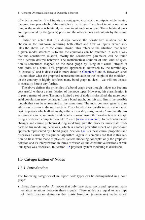
• Reversible transducers: In case the relations of a TF or GY are linear, the opera-tor is a constant matrix that is anti- or skew-symmetric due to power continuity.In case the inputs are independent functions of time (externally modulated MTFor MGY) the anti-symmetric matrix is time variant. In both cases the transduc-tion is reversible in the sense that the sign of the power of each of the ports isalways unconstrained, in other words: power can flow in both directions. In caseof two-ports the matrix is a 2 × 2-dimensional anti-symmetric matrix that hasonly one independent parameternfor the TF or r for the GY:
[e1
f ′2
]
=[
0 n (·)−n (·) 0
][f1
e2
]
(1.2)
or
[e1
e′2
]
=[
0 r (·)−r (·) 0
][f1
f2
]
(1.3)

1 Concept-Oriented Modeling of Dynamic Behavior 15
By changing the positive orientation of one of the ports, the two constitutiverelations of the two ports can be simplified into
e1 = n (·) e2 (1.4)
and
f2 = n (·) f1 = − f ′2 (1.5)
for the transformer and
e1 = r (·) f2 (1.6)
and
e2 = r (·) f1 = −e′2 (1.7)
for the gyrator (Fig. 1.5).
Fig. 1.5 Transformer andgyrator representation ..
n
..r
e1
e1
f1 f2
e2
e2 = –e2’
f1 f2 = –f2’TF
GY
• Junction nodes: A junction is a node with power ports that is power continuousand of which the ports are mutually exchangeable without changing its nature:this property is called ‘port symmetry.’ Scattering variables can also be used toprove that there exist only two types of power continuous, port symmetric nodes,both with linear constitutive relations (i.e., linearity is not assumed a priori) [9]:
(1) A 0-junction or zero-junction (node label: 0) of which the efforts of all portsare equal
ei = e j ∀i �= j (1.8)
and the sum of the flows of all ports with a sign in the summation dependenton the direction of the half arrow of the bond connected to the port beingzero
n∑
i=1
εi fi ∀εi ∈ {−1,+1} (1.9)

16 P.C. Breedveld
where the minus sign holds for bonds oriented away from the junction andthe plus sign for bonds oriented toward the junction.
(2) A 1-junction or one-junction (node label: 1) of which the flows of all portsare equal
fi = f j ∀i �= j (1.10)
and the sum of the efforts of all ports with a sign in the summation depen-dent on the direction of the half arrow of the bond connected to the portbeing zero
n∑
i=1
εi ei ∀εi ∈ {−1,+1} (1.11)
where the minus sign holds for bonds oriented away from the junction andthe plus sign for bonds oriented toward the junction.
As a consequence, all other power continuous nodes are port asymmet-ric. Another result is that modulation of junctions can only take place inthe form of a boolean variable that activates or deactivates the node: thejunction is then called a switched junction (node labels X0 and X1). Thisallows a variable interconnection structure.
Note that junctions fall into the category of non-mixing, reversible trans-ducers. They may be seen as a TF or MTF with a constitutive matrix thatcontains only 1, −1, and 0 as matrix elements and modulation consists ofchanging the absolute values of this matrix. Furthermore, the same holdsfor multiport substructures that only contain junctions. The transpose ofthis matrix relates the independent voltages to the dependent ones and thuscorresponds to those columns of the reduced incidence matrix of an electri-cal circuit that relate the link voltages to the branch voltages.
• Irreversible transduction nodes: An irreversible transduction node is a resistivenode with true power ports with one additional power port of which the flow isequal to the entropy production function of the resistive node. Consequently theconjugate effort equals the power of this port divided by the entropy productionfunction and is called temperature. This illustrates the nonlinear nature of itsconstitutive relations, such that the earlier conclusion that linear, time-(in)varianttransducers are reversible is not violated. Node label: RS. In case of modulation(time variance of the entropy production function): MRS. Note that an (M)RSis an extension of an (M)R and when discussing port-based modeling, it willturn out that the (M)R rather is a special case of an (M)RS which is the resultof a modeling assumption (constant temperature or irrelevance of temperaturechanges) that remains often implicit.
As explained earlier, nonlinearity may be created by port modulation. There-fore, it is possible to use port modulation on an MTF or MGY to create irre-versible behavior, similar to that of the RS. While modeling physical systems

1 Concept-Oriented Modeling of Dynamic Behavior 17
this may have the disadvantage that the irreversibility is hidden in the modula-tion, while designing physical systems with desired behavior it may lead to novelapproaches, e.g., damping with reduced generation of heat. Also, this equivalenceshows that the constitutive relation of an irreversible transducer has a multiplica-tive form and does not violate our earlier conclusion as a consequence.
In case the resistive port of the RS has a linear relation (the entropy producingport always has a nonlinear relation that relates either the rate of change of theentropy or the temperature to the two independent variables of the RS), the two-port RS can be characterized by just one parameter R:
⎧⎪⎨
⎪⎩
e = R f
fSirr =R f 2
T
or
⎧⎪⎨
⎪⎩
f = e
R
fSirr =e2
RT
or
⎧⎪⎨
⎪⎩
e = R f
T = R f 2
fSirr
or
⎧⎪⎪⎨
⎪⎪⎩
f = e
R
T = R f 2
fSirr
(1.12)
1.3.4 Basic Elements
We now have nine basic bond labels: (M)C, (M)I, (M)Se, (M)Sf, (M)R(S), (M)TF,(M)GY, (X)0, and (X)1, which, for reasons of clarity can also be introduced bottom-up, in the sense that each is defined in the simplest form possible and where portsare power ports (as mentioned before, in case ports are not power ports, bond graphsare commonly addressed as pseudo-bond graphs with pseudo-bonds). This simplestform is the minimum number of ports and a minimum number of constitutive param-eters, which results in the linear form. This results in one-port C, I, Se, Sf, and R, aswell as the two-port TF, GY, and RS that are all characterized by one parameter andthe 0- and 1-junctions, which are always linear, have no parameter at all. Junctionsshould have at least two ports to be power continuous, but that would limit thepossible structures to chains only. This means that the simplest form of a junctionrequired to be able to build arbitrary structures should have a minimum of threeports. In case the constitutive parameter of an element is replaced by a functionof time, the modulated and switched versions of the basic elements, i.e., MC, MI,MSe, MSf, MR(S), MTF, MGY, X0, and X1, are obtained (cf. Table 1.3).
Note that Paynter [2] originally used only one-letter labels for the node types:E instead of Se, F instead of Sf, T instead of TF, and G instead of GY. His stu-dents Karnopp and Rosenberg [8] noted that interpretation became easier when insome cases two- and three-letter labels were used and they introduced the label-ing used herein. In some dialects, e.g., [12], the 0- and 1-junctions are replacedby e- and f -junctions (common effort and common flow junction, respectively) oreven using the domain-dependent symbols of effort and flow, like u for commonvoltage junction, v for common velocity junction, and T for common temperaturejunction. Thoma [13] uses a dialect that violates our earlier attempt to only focus atthe topological structure of relations between concepts: he uses the so-called s- andp-junctions, where he relates an s-junction to a series connection and a p-junction

18 P.C. Breedveld
Table 1.3 Basic node types
Node label Linear (time-variant) constitutive relation
M)C e − C−1 (·) q = 0; q = ∫f dt
(M)I f − I−1 (·) p = 0; p = ∫edt
(M)Se e = e (·) ; ded f = 0
(M)Sf f = f (·) ; d fde = 0
(M)R(S) e − R (·) f = 0;(
fSirr − R (·) f 2
T = 0
)
(M)TF e1 − n (·) e2 = 0; f2 − n (·) f1 = 0
(M)GY e1 − r (·) f2 = 0; e2 − r (·) f1 = 0
0 ei = e j ∀i �= j;n∑
i=1εi fi = 0 ∀εi ∈ {−1,+1}, +1: inward; −1: outward
1 fi = f j ∀i �= j;n∑
i=1εi ei = 0 ∀εi ∈ {−1,+1}, +1: inward; −1: outward
X0 ei = if condition then e j else 0 endif ∀ j �= i ;
f j = if condition thenn−1∑
i=1εi fi ∀i �= j, εi ∈ {−1,+1} else 0 endif
X1 fi = if condition then f j else 0 endif ∀ j �= i ;
e j = if condition thenn−1∑
i=1εi ei ∀i �= j, εi ∈ {−1,+1} else 0 endif
to a parallel connection. Given that this only has a meaning for physical structuresand confuses a topological representation of concepts with a spatial representation,we strongly advise against the use of the terminology in this dialect, as it causes aform of confusion during physical systems modeling that can be quite misleading.
Again it is emphasized that although the terminology (power, energy, entropy,and temperature) seems to imply a link with the physics, the link with the corre-sponding physical concepts like energy and power will be made during the dis-cussion of port-based modeling. This section lists unambiguous definitions of themost elementary node types. However, any user can add specific nodes to thesedefinitions. The answer whether it makes sense in the context of port-based mod-eling does not belong in the framework of the description of the notation itself: itis possible to express both sense and nonsense in terms of correct language, andbond graphs are nothing more or less than a graphical language of which we arediscussing the semantics and grammar rules. In Section 1.4 we add causal port prop-erties and causality assignment to set the stage for using this graphical language inphysical system modeling, but first we shortly discuss how an existing model can betranslated or transformed into a bond graph. In Section 1.5 it will become clear thataspects of the causality assignment procedure can also be used during the processof modeling itself as they provide immediate feedback on the modeling decisionsbeing taken.

1 Concept-Oriented Modeling of Dynamic Behavior 19
1.3.5 Model Transformation into a Bond Graph
When a model is already available in the form of a domain-dependent iconicrepresentation like an electrical circuit diagram or a mechanical schematic,it can be converted into a domain-independent bond graph by first identify-ing the domains that are present (step 1) and choosing a reference effort (orvelocity) (step 2), next identifying all the port types that are present (step 3)and listing to which effort or effort difference (velocity or velocity difference)they are connected (step 4). All efforts can be represented by a 0-junction(step 5) and all effort differences can be represented by a 0-junction that isconnected to the two 0-junctions of which it is a difference by means of a1-junction and bond orientations that result in this difference (step 6). Similarly,all velocities can be represented by a 1-junction (step 5) and all relative velocities(‘velocity differences’) can be represented by a 1-junction that is connected tot thetwo 1-junctions of which it is a difference by means of a 0-junction and proper bondorientations (step 6). Finally all ports can be connected to this junction structureusing the list made during step 4 (step 7). Finally superfluous junctions can beomitted (junction structure simplification; step 8) [14, pp. 297–311]. These eightsteps can be used to perform model transformation.
Take, for instance, the model represented in Fig. 1.6 by an iconic diagramwhich shows an ideal planar pendulum driven by an electric dynamic transducer(motor/generator) connected to a voltage source. The model has four domains inthe mechanical framework of variables that we will use, viz., the electromagneticdomain, two orthogonal mechanical translation domains, and the rotational domain.In the thermodynamic framework it would have eight domains, viz., electric, mag-netic, three potential, and three kinetic domains for each of the two independentcoordinates of the plane as well as the rotation in that plane, but as the iconicdiagram model is already based on the mechanical framework of variables, wechoose to work herein and show the transition to the thermodynamic frameworklater. Hence four references (in the mechanical case: reference directions) need tobe identified: the electric ground as indicated in the iconic diagram as well as thereference frame with the orthogonal velocities in the x- and y-directions that spanthe plane and the angular velocity in that plane. The already identified elementarybehaviors in the electromagnetic domain are (cf. Fig. 1.6) an ideal voltage source,the series resistance of the current loop, i.e., mainly of the motor windings, the series
ys
yb
xs
xbm
g
us
Re
Km
L
b ϕ
ω
J
Fig. 1.6 Iconic diagram of example model
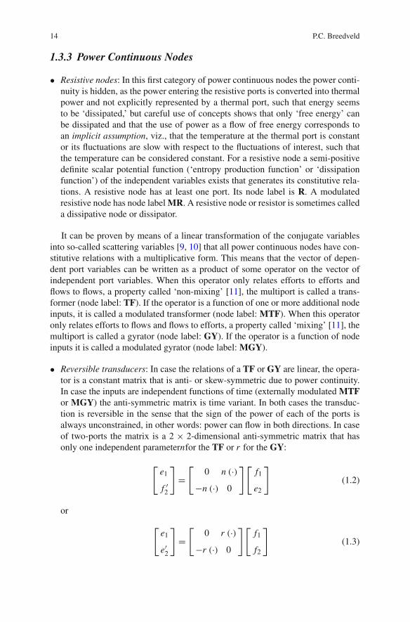
20 P.C. Breedveld
inductance of the motor windings, and the electric port of the ideal motor/generator(magnetic field assumed to be constant!). The other port of the motor is in therotational domain, in which also the motor inertia and the bearing friction can beidentified in the iconic diagram. The symbol for the pendulum mass indicates thatit is assumed to be a point mass with I-type storages in both coordinate directions.If one of these directions is in parallel with the gravitational acceleration, the iconicdiagram expresses that there is a constant force of effort (force) on the correspondingI-type port, which corresponds to an Se-type port.
What remains to be done is to translate the configuration information of the pen-dulum, i.e., the rigid constraint between the pivot point and the point mass
x = l cosϕ (1.13)
y = l sinϕ (1.14)
u12 u23
u12
us u1
u23
u1 u2 u3
u2 u3
0 0 0 1
1
1
0 0
1 1ω
vx
vy
0 0 0 1
1
1
0 0
1 1Se
R I L
GYKm
MTF
I
I
Se–mg
ϕ
ω
vx
vy
mx
my
cosϕ
Re
0u1 u2 u3
0 0 1ω
1vx
vy
1a:
b:
c:
I J R b − sinϕ
us
–mg
Re
d: 1ω
1
1i
Se
R I L
GYKm
I J R b I mx
vy
myI
Se
ϕ
MTF
MTF
− sin(ϕ)
cos(ϕ)
Fig. 1.7 Intermediate steps (a–c) and final bond graph (d) of the example

1 Concept-Oriented Modeling of Dynamic Behavior 21
into velocity relations that generate the remaining part of the junction structure thatfor the time being can be modeled as a three-port position-modulated transformer(with ϕ being the modulating state) with flow relations:
x = (−l sinϕ) ϕ (1.15)
y = (l cosϕ) ϕ (1.16)
and due to the necessity of power continuity of the constraint:
Tϕϕ = Fx x + Fy y = (−l sinϕ) Fx ϕ + (l cosϕ) Fy ϕ (1.17)
The torque force relation should be
Tϕ = (−l sinϕ) Fx + (l cosϕ) Fy (1.18)
resulting in the 2× 1 transformation matrix
[−l sinϕl cosϕ
]
(1.19)
that characterizes this 2× 1-port MTF.Via the intermediate steps mentioned above (cf. Fig. 1.7a–c) and a straightfor-
ward decomposition [15, 16] of the 2× 1-port MTF into two elementary MTFs thefinal bond graph in Fig. 1.7d is obtained.
1.4 Computational Causality and Causality Assignment
1.4.1 Introduction
Although there are physical arguments for some of the causal port properties, thissection will only address the possible causal port properties and a causality assign-ment algorithm that is based on these properties. The implications on physicalsystem modeling will be discussed later. The aim of this particular algorithm is togenerate a computational structure that is optimally suited for computer simulation,but other algorithms can be defined that have other purposes.
Each port in a true bond graph is characterized by four relevant objects: effort,flow, power, and the constitutive relation between effort and flow that may containan integration or differentiation with respect to time. In case of pseudo-bonds thereare only three relevant objects, effort, flow, and constitutive relation, as the conju-gation of effort and flow is not related to power. In case of linearity, the constitutiverelation is characterized by just one parameter per port. It depends on the purposeof the model that is being represented by the bond graph which of these objectsare independent and which are dependent with respect to a particular port. If theconstitutive relation is a known and therefore independent object, either the effort

22 P.C. Breedveld
or the flow has to be an independent variable due to the definition of a constitutiverelation, while the (power) conjugate variable is by definition dependent. As a result,the power is a dependent variable too, because it is equal to the product of the powerconjugate variables effort and flow. When the constitutive relation is the dependentobject – as is the case in the context of design or parameter estimation – both theeffort and the flow can be considered independent objects of a port.
Hence, we can distinguish two situations:
1. Known constitutive relation: Either the effort or the flow is an independent vari-able, power can always be computed as the product of effort and flow
2. Unknown constitutive relation: Both effort and flow are independent variables
In the first case the effort and flow can be considered bilateral signals at the port(cf. Fig. 1.4). Consequently, the bond connected to that port represents a bilateralsignal flow and at the port at the other side of the bond, the roles of effort and flowin the constitutive relation of that port are reversed.
While a bond graph is being constructed a choice has to be made for each portbetween independent (input) and dependent (output) port variable. If the effort ofa bond serves as the input for one of the two ports it connects, it has to be theoutput of the other port. Due to the bilateral nature of the connection the flow ofthe first port has to be an output and serves as an input for the second port. Whena choice is made, this is indicated in the bond graph by a causal stroke at the endof the bond that is connected to the port where the effort is an independent variableand the conjugate flow a dependent variable. As a result, the open end of the bond(i.e., the end without a causal stroke) is connected to the port where the flow is anindependent variable and the conjugate effort a dependent variable (Fig. 1.4). Whena bond graph is ready and fully augmented with causal strokes, it can be automat-ically converted into a set of computable assignment statements. The assignmentof this computational causality or, if no confusion is possible, just causality is analgorithmic process based on the causal properties of each port and/or node type[8, 17]. The graphical representation of this computational structure also gives amodeler immediate feedback on his modeling decisions [18].
In the second case it is possible that at some port both effort and flow are inde-pendently given and the constitutive relation (the constitutive parameter of the linearcase) is the dependent object. As mentioned before, this situation has been addressedin the literature as ‘bi-causality’ (cf. Chapters 5 and 6). The concept of bi-causalitymay play a role in design and identification of unknown constitutive relations. Insome dialects it is represented by drawing only the upper half of the causal strokeat the port where both effort and flow are given and by putting the lower half of thestroke at the other side of the bond, assuming that the bond is drawn horizontallyto be able to explain the position in terms of ‘upper’ and ‘lower.’ Naturally theorientation of a bond in the drawing plane of the graph has no meaning as it istopological, so the concept of ‘lower’ will be defined with respect to a bond inthe side of the bond where the little stroke of the half arrow is located. Obviouslythe concept of ‘upper’ is the other side of the bond. It is clear that in a context ofmodeling existing dynamic behavior with the purpose of numerical simulation thesituation that a constitutive relation is unknown is not relevant and is merely used for

1 Concept-Oriented Modeling of Dynamic Behavior 23
computational purposes related to design and parameter estimation/identification inwhich one may have doubts about the added value of graphical representation in abond graph. For this reason, only the first case will be considered in the remainderof this section.
1.4.2 Causal Port Properties
Ports may have different causal properties:
(1) The causality of the port is fixed. This occurs in two situations:
(a) Either the effort or the flow is a given input of the port, independent of theconjugate variable. This corresponds to the definitions of the (M)Se andthe (M)Sf nodes.
(b) The constitutive relation has a form that can only be made explicit in onecausal form (non-invertible) any other node except the junctions.
(2) There is a preference for a particular causality. For example, in case there isa preference for integration over differentiation with respect to time, the portsof the storage nodes, (M)C and (M)I, may be given a preferred causality, viz.,effort-out (C) and flow-out (I), respectively. This will turn out to be the mostcommon preferred causality later, when a causality assignment algorithm is dis-cussed aimed at generating a set of differential equations that is in an optimalform for numerical simulation.
(3) There is a constraint between the causality of two or more ports of a node. Thisis the case for the elementary two port nodes (M)TF and (M)GY: the (M)TFalways has only one stroke at the node, while the (M)GY has either both strokesat the node or both open ends. The junctions also have such a causal constraint:an n-port 0-junction has one stroke at the node and n − 1 open ends, while ann-port 1-junction has one open end at the node and n − 1 causal strokes. Thesame holds for the X0 and the X1 in principle, but in many cases they will begiven a fixed causality, given the discontinuous and consequently non-invertiblenature of their constitutive relations.
(4) In all other cases there is arbitrary causality or free causality, which means thatthe causality can be chosen freely or is determined by the causal properties ofthe port at the other side of the bond.
1.4.3 Causality Assignment
Causality assignment or causal augmentation is an algorithmic procedure that canbe applied to a bond graph based on the causal port properties of its nodes. Animportant process during this assignment is the propagation of causality via causalconstraints. This means that when the port of a node with constrained causal portproperties gets its causality assigned in such a way that it determines the causalityof one or more of its other ports on the basis of the constraint, the causality is

24 P.C. Breedveld
propagated via these other ports, which in turn can cause propagation at the othernodes to which these ports are attached until the process stops. The causal bondsresulting from such a propagation process form a so-called causal path. Whencausality propagation results in a closed causal path or causal cycle, in most cases aglobal constraint can be applied on that cycle that depends on the particular domainrepresented by the graph.
In short, the following steps are taken:
(1) Choose an unassigned port with a fixed causality of type 1a, assign it, and checkthat the causality of the port at the other side of the bond, which is assigned asa result
(a) either is not in conflict with a fixed causality of that port: If there is aconflict with a fixed causality of type 1a, the bond graph is ill-posed; ifthere is a conflict with a fixed causality of type 1b, the constitutive rela-tion should be changed into an invertible one or approximated by iterationduring numerical solution, or
(b) corresponds to the preferred causality of that port: If not, the consequencesshould be checked based on the origin of the preference, or
(c) is propagated via the causal constraint of the port of the other side of thebond to one or more ports for which all these checks should be repeateduntil propagation ends, or
(d) is an arbitrary or free causality.Continue with (1) until all ports with fixed causality of type 1a are
assigned.
(2) Choose an unassigned port with a fixed causality of type 1b, assign it, and checkthat the causality of the port at the other side of the bond, which is assigned asa result
(a) either is not in conflict with a fixed causality of that port: A conflict witha fixed causality of type 1a cannot occur here, as it should have becomeapparent during step 1; if there is a conflict with another fixed causalityof type 1b, one of the two constitutive relations should be changed into aninvertible one, approximated by iteration or the resulting combination ofinvolved constitutive relations should be rewritten analytically, or
(b) corresponds to the preferred causality of that port; if not, the consequencesshould be checked based on the origin of the preference: preferably the con-stitutive relation should be changed as assigning a non-preferred causalityin this manner unnecessarily decreases the order of the set of state equationsrepresented by the bond graph, or
(c) is propagated via the causal constraint of the port of the other side of thebond to one or more ports for which all these checks should be repeateduntil propagation ends, or
(d) is an arbitrary or free causality.Continue with (2) until all ports with fixed causality of type 1b are
assigned.

1 Concept-Oriented Modeling of Dynamic Behavior 25
(3) Choose an unassigned port with a preferred causality, assign it, and check thatthe causality of the port at the other side of the bond, which is assigned as aresult
(a) either corresponds to the preferred causality of that port; if not, this meansthat the corresponding states are not independent of each other (in case ofintegral preferred causality) or that the states or not independently control-lable (in case of differential preferred causality), or
(b) is propagated via the causal constraint of the port of the other side of thebond to one or more ports for which all these checks should be repeateduntil propagation ends, or
(c) is an arbitrary or free causality.Continue with (3) until all ports with preferred causality are assigned.
If all bonds have obtained their causality after this step a set of ordinarydifferential equations (ODE) is obtained, if not, the result will be a set ofmixed differential and algebraic equations (DAE).
(4) Choose an unassigned port with an arbitrary causality, choose a causality, andcheck that the causality of the port at the other side of the bond, which isassigned as a result
(a) either is propagated via the causal constraint of the port of the other sideof the bond to one or more ports for which all these checks should berepeated until propagation ends, or
(b) is an arbitrary or free causality too; make an inventory of all the algebraicloops that occur as a result of the first choice and compare it with theproperties of the algebraic loop(s) that would occur when the first choicewould have been different. If solution of the algebraic loops by iterationis no option, the set of constitutive relations that is part of the causal pathcan be written in an explicit form analytically. Note that the choice of thearbitrary causality may influence the loop gain of the algebraic loop andmay be adapted to obtain a set of algebraic relations that is optimal fornumerical solution.
Continue with (4) until all ports with arbitrary causality are assigned.
1.4.4 Causality Assignment Example
Straightforward application of the causality assignment to the bond graph in Fig. 1.7results in Fig. 1.8, where the numbers refer to the sequential order in which thecausal strokes were assigned. Note that the two I-type storage elements representingthe pendulum point mass do not get their preferred causality. Section 1.5 will explainand solve this issue.
A causal bond graph is commonly synonymous with a set of ordinary first-orderdifferential equations (ODE) that can be automatically generated from the graphwhen the constitutive relations of each port are well defined (linear relations are

26 P.C. Breedveld
Fig. 1.8 Causalityassignment to bond graph ofexample model
1ω
1vy
1i
Seus
R Re I L
GYKm
I J R b I mx
I my
Se–mg
ϕ
MTF
lcos(ϕ)MTF
–lsin(ϕ)
1
2
3
4
5 6
7
89
10
11
12
13
used by default). In case dependent storage ports or algebraic loops are detectedduring causality assignment, like in Fig. 1.8, the user knows that the generatedset of equations is a mixed set of differential and algebraic equations (DAE) inprinciple – automated symbolic processes may still generate a set of ODE’s –such that an appropriate choice of a numerical integration method has to be made[19]. Modeling and simulation tools like 20sim can make efficient use of theseaspects (www.20sim.com), such that a first simulation result of a modeling idea or adynamic effect on a model change can be easily obtained, thus providing fast feed-back on modeling decisions, which improves the modeling and model debuggingprocesses.
1.5 Port-Based Physical System Modeling
1.5.1 Introduction
Modeling can be defined as the creation of an abstraction of a (part of a) problemand its context in such a way that the abstraction helps the modeler deal with thatproblem, where a problem should be considered in the most general sense of theword: the need for more insight can be seen as a problem as well. Obviously, there isno such thing as THE model, as each modeler will make his own modeling decisionsand it is highly unlikely that these are always the same. Furthermore, even though aman-made device may have been constructed from the perspective of one particularfunctional model, the context of its physical realization will rarely be identical, suchthat different models are needed that depend on a particular context. This means thatit makes no sense trying to find out if one particular model is ‘true’ or ‘false’: thekey issue is whether or not the model is competent to help the modeler answer hisquestion in the most general sense of the word. In many cases this competence canbe quantified by the error between the numerical results of a model and measure-ments of relevant aspects in the real world that the model tries to capture. However,in some cases a qualitative correspondence in the sense of the nature of the behavior(e.g., oscillation, relaxation, and (in)stability) may already lead to the solution of aproblem without considering numerical errors.

1 Concept-Oriented Modeling of Dynamic Behavior 27
1.5.1.1 Intended Behavior Versus Parasitic Behavior
In case a model needs to be created for trouble-shooting purposes of a man-madedevice with an intended functional behavior, the designer of that device is oftennot the most successful modeler as the problems often result from the differencebetween the behavior of the actual physical realization and the conceptual picture ofreality that the designer used to create a particular functionality and that is a modelas well. The trouble-shooter should model the physical effects that are ‘parasitic,’i.e., not contributing to the intended functionality. Parasitic effects are effects thatare neglected initially, yet influence the behavior in such a way that they should beincluded in a model to be able to capture the behavior that is of interest. They shouldbe made part of the model in order to be able to solve the problem at hand.
1.5.2 Basic Physical Principles
In case of the general context of physical systems, i.e., systems of which the behav-ior is supposed to obey the basic principles of (classical) physics, a model of thedynamic behavior of a physical system is also supposed to correspond to these basicprinciples like energy conservation, and positive entropy production and the conser-vation principles of the generic physical quantities like momentum, electric charge,magnetic flux (linkage), and entropy (while allowing that entropy is produced aswell!). These principles can be considered generic modeling assumptions.
1.5.3 Modeling Versus Model Transformation
Many textbooks that claim to discuss modeling ‘pollute’ the picture of modelingsketched above, as they do not describe the process of modeling itself, but theprocess of transforming one model description (usually in the form of natural lan-guage supported by sketches or diagrams) into another one, usually in the form ofa set of (differential) equations or a block diagram representing a computationalstructure or even the input code of a specific simulation package. The modelingdecisions themselves, i.e., the decisions about the physical phenomena that shouldbe represented by the model in order to obtain a competent description of realityin a particular problem context, commonly do not play a large role. For instance,when Feynman et al. [20] in his Lectures on Physics part 1 Fig. 4.7 shows a pendu-lum, his text makes clear that his ‘pendulum’ is already a model consisting of idealconcepts: a point mass, an infinitely stiff, massless constraint, and an ideal pivotpoint. The transformation into equations then becomes a process with a uniqueresult. Zill [21, p. 209] makes a difference between a ‘physical pendulum’ – anyobject that swings back and forth – and a ‘simple pendulum’ for which he explicitlystates most assumptions. However, his concept ‘mass’ is implicitly assumed to bea point mass and his concept ‘rod’ is implicitly assumed to be infinitely stiff. Hethen generates the corresponding differential equation (= model transformation)

28 P.C. Breedveld
by writing the constraint of the rod in terms of accelerations and relates this viaNewton’s second law to the tangential force. By referring to his sketch he equatesthis force to the tangential component of the gravitational force and thus obtainsa nonlinear second-order differential equation in the angular displacement of thependulum from its equilibrium position. No attention is paid to the background ofthe modeling decisions when they cease to lead to a competent model and this istypical for many descriptions of a modeling process.
The transformation of the iconic diagram of the simple pendulum model intoa second-order differential equation is unique, given a choice of relevant variables(angular, tangential, horizontal, or vertical displacement) and parameters (pendulumlength and mass, gravitational acceleration). It is a suitable exercise in model trans-formation for engineering students, but has nothing in common with the modelingprocess itself, i.e., the decision under which circumstances this model is a compe-tent abstraction from reality that helps answer a question. As it is easier to createan appearance of objectivity in exams by testing model transformation abilities onthe basis of one possible result, while model decisions are much less strict and bydefinition subjective to some extent, most educational systems that have deviatedfrom the master–pupil model for efficiency reasons have also deviated from teachingthe actual process of modeling as a consequence.
Before the time of computer simulation, many could counter this criticismby demonstrating that bringing in more complex aspects into a model leads todifferential equations that cannot be solved analytically, giving not much room forcompetence to help to solve a problem. In other words, the availability of solv-able model structures was relatively small and the decision process restricted tothe selection of a model structure that would best capture the data. However, usingcomputer simulation, the behavior of much more complex models can be studied,which means that carefully taken modeling decisions and explicit assumptions are akey to competent models for real-world situations.
1.5.4 Model Representations
Apart from mathematical model representations in terms of differential equations,many graphical model representations exist: block diagrams and signal flow graphsare used to represent the mathematical structure of a model, Venn diagrams and Petrinets represent the logi(sti)c structure of systems in which the events are consideredto be discrete in time, electrical circuit diagrams represent both the relations betweenthe electrical properties of physical components and the relations between concep-tual elements. Iconic diagrams similar to circuit diagrams exist for the mechanic,hydraulic, pneumatic, and thermal domains, even though the symbols are often notas well defined as in the electrical case, the picture of a simple pendulum modelbeing an already used example. In all cases, however, the (arbitrarily) chosen metricof the topological graph has no meaning: The location of the nodes with respect toeach other is commonly chosen such that the picture gives an organized impression.

1 Concept-Oriented Modeling of Dynamic Behavior 29
Fig. 1.9 Simple electricalcircuit diagram
For instance, in an electrical circuit diagram the unwritten, heuristic rule is thatthe reference node is at the bottom, nodes related to sources at the left, and nodesrelated to loads at the right, while the nodes are kept as much as possible at a gridand the symbols of the labeled edges are connected to the nodes by straight lines(Fig. 1.9).
By contrast, in a linear graph [22], which can be seen as an abstraction of a circuitdiagram, the edge symbols are replaced by edge mnemonic codes that are not part ofthe edge anymore, while the edges are commonly drawn as curved lines. In his ear-lier mentioned lecture with the challenging title ‘complete breakdown of intuition,’Lewin incorrectly implies that the arbitrary area enclosed by the edges of a circuitdiagram can be related to an actual area enclosed by a current-carrying wire, a cur-rent that can be (among other things) the result of a magnetic field surrounded by thiswire. Note that the arbitrary area is only present in the graph in order to represent thenodes separate from each other and that the layout can be changed without changingits meaning. The influence of a magnetic field on an actual (‘spatial’) area enclosedby actual wires thus has to be separately represented in a graph (circuit diagram)by the concept of an ideal inductor (‘conceptual concentration’), which would haveprevented the paradoxal conclusions Lewin makes and which even makes him statethat ‘Kirchhoff is for the birds.’ Even though this may have been an educational trickto draw the attention of the audience, downplaying famous scientists like Kirchhoffand even downplaying his own colleagues of whom he says in a suggestive way thattheir correct claim that he is cheating ‘is telling you something about them’ doesnot seem to fit in this explanation. The point where he is actually cheating is whenhe claims that the voltmeters are connected to the same points: he has connectedthe voltmeters to different points in space, viz., immediately across the spatiallyseparate resistors, interpreting the wires as ideal connectors which can then be con-sidered to be ‘the same points’ from the perspective of electric potentials. However,the wires between these points constitute the majority of the winding that picksup the induced current, thus generating an induced voltage between his points ofmeasurement. Like one of the comments on YouTube puts it: ‘There is no problemin interpreting the flux term in Faraday’s equation as an EMF, it is done historicallyand everyone knows that is not a gradient of a scalar potential.’ (EMF stands herefor electromotive force, the induced voltage, and is often called back-EMF whenthis voltage is generated by a spinning motor and thus a measure for its speed.)
The reason for spending so many words on this issue is that these kinds of con-fusions are deeply rooted in our scientific culture. A good way to prevent oneselffrom falling into the traps of confusing modeling with model transformation, of

30 P.C. Breedveld
confusing spatial information with a topology representing conceptual structure andunjustified extrapolation of existing models is to use the following checklist:
Checklist for modeling physical systems:
• Make problem context explicit as much as possible and iterate at any time whenneeded
• Make implicit assumptions explicit• Keep record of all assumptions being made• Keep the spatial configuration information separate from the topology that repre-
sents conceptual structure, even if the variables happen to coincide
Note that the example of the model with the ideal pendulum in Fig. 1.6 is anexample of a situation where the position variable (the angular position ϕ) merelydescribes a configuration state.
Next we study the conceptual foundations of each dynamic model.
1.5.5 The Concepts of System Boundary and Environment
The system boundary separates the system or subsystem from its environment. Theenvironment of a system is that part of the rest of the universe that has some form ofrelation with the system. The environment can influence the behavior of the system,but not its dynamic characteristics. The system boundary is the boundary between asystem and its environment that can be defined on the basis of a boundary criterion.Common boundary criteria are based on the concept of state that will be discussedfirst.
1.5.6 The Concepts of State, Equilibrium, and Change of State
All dynamic models are based on the concept of state. States can be divided intoextensive states, i.e., states that are proportional to the extent (either spatial, mate-rial, or both) of the physical object of which the behavior is described, and inten-sive states, i.e., states that are independent of the extent of this physical object.An extensive state can be related to a conservation principle (momentum, charge,matter, magnetic flux, displacement, etc.), i.e., if q is a state it satisfies the property∮
dq = 0, and its dialectic complement, the ‘rate of change of state’, dq/dt = fis generally considered a flow of the corresponding quantity in a general sense, asconservation is also interpreted in the sense that an exchange of a stored quantity hasto take place via the intermediate space. In other words it is assumed that conser-vation is not achieved by simultaneous annihilation and generation at the same rate.The state and its rate of change are considered dialectic complements as a state hasno meaning when it cannot change and a flow has no meaning if it does not resultin change of state, even when this state is not included in the model. The latter

1 Concept-Oriented Modeling of Dynamic Behavior 31
remark refers to the situation that storage of ‘what is flowing’ is not always rele-vant to understand behavior. This is the case when constant (= ‘stationary’) flowsplay a role in a model. In other words, flows can exist that describe an exchangewith a non-storing concept, i.e., they are not identical to a rate of change of state,although they may contribute to it. This process of shaping concepts can be seen as‘conceptual concentration’: even though the flow is in principle always related to achange of state, it may be decoupled from it by concentrating the change of statein a particular concept (‘storage’) and concentrating the description the contribu-tion to the change of state in a separate summation of contributions, i.e., flows thatare not a time derivative of a state individually, but contribute to it via a so-calledbalance equation. This approach allows that the storage related to flows is not partof the model, but of the environment, such that there is no need to describe it asstorage.
A system is said to be in its equilibrium state when the system is not exposedto changing environmental influences (there may be a constant influence though)and all the rates of change of state are zero and consequently all states constant.This means that flows can be considered ‘equilibrium-establishing variables’: thenet result of contributing flows to a rate of change of state is unequal to zero untilthe equilibrium state is reached. This leaves room for some flows not being zero,but having a constant value in equilibrium. In other words, the concept of a flowcan be generalized by realizing that each contribution to a rate of change of state ina balance equation can be considered a flow, such that a flow itself does not haveto be equal to a rate of change itself. This means that an equilibrium situation canoccur if the sum of the non-zero, constant flows in a balance equation results in azero rate of change of state. Such a special case of equilibrium is called a stationarystate.
When a state of an object is identified, it is considered the same for the wholeextent of the object or concept being considered. The extent itself is also a state, eventhough it is often constant. When we increase the extent by bringing two objectstogether that are in mutual equilibrium, i.e., do not result in flows when left tointeract freely with each other, the intensive state remains the same by definition.In other words, the equilibrium between two objects is determined by the intensivestates being equal. On the other hand, a difference in intensive state(s) will generate(a) change(s) of state or flow(s) until an equilibrium is reached. This brings us to theheart of the description of dynamic physical processes: flows that establish equilib-rium and intensive states or efforts that determine equilibrium and thus can be con-sidered ‘equilibrium-determining variables.’ As a consequence, efforts and flowsare said to be dynamically conjugated. Note that this distinction for the concepts ofeffort and flow is available for a thermodynamic type of variable classification (cf.Table 1.1). We will see later that this distinction is lost in the mechanical frameworkof variables (cf. Table 1.2) where the potential and kinetic domains are combinedinto one domain, which is unfortunate for the process of identifying concepts duringmodeling. Combined with checks of units and dimensions, the check on the natureof physical variables forms a powerful instrument for taking modeling decisions andchecking the consistency of models.

32 P.C. Breedveld
1.5.7 Boundary Criteria
The states that are commonly used as boundary criteria are ‘amount of matter,’ e.g.,not only the fixed amount of matter in a rigid body, but also a fixed amount of fluid inLagrangian coordinates or the gas in a closed balloon, and ‘available volume’, e.g.,not only a container with a fixed volume, but also a ‘control volume’ for the studyof fluid flow in Eulerian coordinates. In case of the ‘matter criterion’ the systemconsists of a fixed amount of matter or rather the boundary is defined as a borderthat does not allow exchange of matter. In case of the ‘volume criterion’ the systemconsists of a fixed volume or rather the boundary is defined by a border that doesnot allow volume changes. Note that the two latter formulations are more generalas they allow mixed boundaries like fluid flowing through a piece of flexible tube:the openings are spatially fixed with respect to the wall boundaries and allow nochange of volume, while they do allow exchange of matter (fluid), while the tubewall does not allow an exchange of matter, but it does allow a change of availablevolume due to the flexibility of the tube. In principle, other conserved quantities likeelectric charge could serve as a boundary criterion too, but this is seldom used.
In case of a spatial structure of components that are modeled as a network struc-ture, the network structure is only constant if the subsystem boundaries maintaintheir relative locations with respect to each other, in other words, each subsystemshould keep the same neighbors. This means that material subsystem boundariescan only be used when they do not violate the network structure. For instance, rigidbodies in a chain structure should not pass each other. In case the volume criterionis used to define a subsystem boundary a similar constraint holds that is automati-cally satisfied if all volume boundaries are defined with respect to the same spatialreference.
1.5.8 The Port Concept
Due to the dynamic conjugation of intensive state (equilibrium-determining variableor effort) and rate of change of extensive state (equilibrium-establishing variableor flow), the concept of a ‘port’ can be introduced as the medium of exchange ofthe concepts effort and flow with other conceptual entities that represent dynamicproperties of physical objects. This way of looking at relationships between physicalconcepts can be seen as a paradigm change with respect to the input–output wayof thinking that is induced by modeling in terms of block diagrams (with fixed,explicit causality) as well as with respect to the completely a-causal description of,for instance, balance equations. The possibility to represent the chosen causality fora port in a bond graph as an algorithmic consequence of a particular interconnection,not only generating a format of the model equations well suited for simulation butalso providing feedback to the modeler about his modeling decisions, is a featurethat makes a bond graph extremely well suited to construct and to represent port-based models.

1 Concept-Oriented Modeling of Dynamic Behavior 33
1.5.9 Bond Graph Construction
A bond graph can be written during modeling in a manner similar to the modeltransformation into a bond graph representation:
Identify domains, choose a reference per domain, and identify commonequilibrium-determining variables. These are commonly efforts, but if the classicalmechanical framework of variables is used the kinetic effort, i.e., the velocity, isdualized into a flow. Represent common efforts by 0-junctions and common veloc-ities by 1-junctions. Identify the basic concepts that are needed to represent therelevant phenomena per domain in terms of ports. For instance, an ideal transformerthat connects two domains has two ports and each of them has to be identified.Next it has to be determined to which effort (velocity) or effort difference (velocitydifference) a port is to be connected. An effort difference can be constructed bymeans of a 1-junction and a velocity difference can be constructed by means of a0-junction, but all effort differences should be explicitly represented by 0-junctions,while all velocity differences should be explicitly represented by 1-junctions. Nextall ports can be connected to 0-junctions (or 1-junctions in case of mechanical ports)and the bond graph can be simplified when possible. Note that the reference effortor velocity is not represented by a junction (as it would result in an unnecessarilycomplex graph that leads to the same result after simplification), unless one is inter-ested in the value of the conjugate variable acting on the reference (e.g., the reactionforce or the ground current).
Returning to the causal bond graph of the example in Fig. 1.8 we can nowconclude that the differential causality of both I-elements results from the rigidconstraint between the rotor inertia and the point mass of the pendulum in thetwo degrees of freedom of the plane. Even without writing equations the mod-eler gets this feedback from causality assignment and since this can be automatedthis provides a means for immediate feedback on modeling decisions while draw-ing the bond graph. It immediately shows that infinitely rigid, massless mechani-cal constraints are in principle not physically realizable, but that it still may be agood decision to neglect the elastic behavior of a stiff mechanical connection asit introduces high frequent behavior in the model that may not be relevant for theproblem context and is at the same time costly for numerical integration. In casethe transformers would have a constant transformation ratio (no modulation), thebond graph allows for a straightforward model transformation of both dependentI-elements to the same junction as the rotor inertia, with which they can be com-bined into one I-element with integral causality, an operation analogous to appli-cation of the Huygens–Steiner theorem (e.g., [23]). However, in case of modu-lated transformers an additional gyristor [24] is generated (cf. Fig. 1.10) for bothx-direction
Tx = (−l sinϕ)d
dt(−ml sinϕ) ϕ = d
dt
(ml2 sin2 ϕ
)ϕ −
(ml2 sinϕ cosϕ
)ϕ2
(1.20)

34 P.C. Breedveld
1
1
1i
R:Re I :L
GY
Km
..
..
....
J :I
b :R
ml2 sin2 ϕ : I*
SeMTFGR
GR
ml2 cos2ϕ : I*l cosϕ
us: Se
..–mg
dϕdt
–(ml2 sin ϕ cos)
dϕdt
–(ml2 sin2ϕ cos)
Fig. 1.10 Virtual inertia’s and gyristors resulting from a transformation of the I-elements to thebody-fixed frame in the example of Fig. 1.7
and y-direction
Ty = (l cosϕ)d
dt(ml cosϕ) ϕ = d
dt
(ml2 cos2 ϕ
)ϕ+
(ml2 sinϕ cosϕ
)ϕ2 (1.21)
However, in this particular case of rotation, the sum of the two time-dependentvirtual inertias becomes a true (constant) inertia
d(ml2 sin2 ϕ
)ϕ
dt+ d
(ml2 cos2 ϕ
)ϕ
dt= dml2ϕ
dt(1.22)
such that the total inertia becomes
J + ml2 (1.23)
and the gyristor contributions compensate each other as a consequence:
−(
ml2 sinϕ cosϕ)ϕ2 +
(ml2 sinϕ cosϕ
)ϕ2 = 0 (1.24)
Note that if the constraint would be elastic, the gyristors (GR) would stay in themodel and represent the fictitious forces like the centrifugal force (in case of a rigidconstraint, the corresponding velocity and thus the corresponding power is zero,such that the contribution becomes irrelevant for the behavior).
The result of transforming both I-elements leaves only the Se-element repre-senting gravity at the other side of the transformer. Taking a closer look at thecombination of configuration state-modulated MTF and Se shows that internal port-modulation results in a nonlinear C-element (cf. Fig. 1.11):
TC = −Tg = − (l cosϕ) Fg = − (l cosϕ) (−mg) = mgl cosϕ (1.25)

1 Concept-Oriented Modeling of Dynamic Behavior 35
1 11
R:Re
R:Re
us :Se
us :Se
I:L
GY..Km
I
b:R
SeMTF
l cosϕ.. ..
–mg
:
11
I
GY
I
R
C
:L
b:
mgl cosϕ
:
..Km
∫a:
b:
J + ml2
J + ml2
Fig. 1.11 Resulting inertia combined with Se via a port-state-modulated transformer (a) resultingin an IC second-order loop and (b) with nonlinear C
The causal path between the I and the C immediately shows the potential peri-odic behavior of the pendulum. For small angles around −π/2 this C-elementeven becomes a linear C-element with parameter 1/mgl and the relation for theoscillation frequency f can be seen directly from the graph to be the commonresult:
f = ω
2π= 1
2π√
IC= 1
2π
√mgl
J + ml2= 1
2π
√g
Jml + l
(1.26)
When compared to immediately writing a damped second-order model in theangle ϕ for the pendulum, one may observe that the final result is identical, but thatthe approach allows for physically motivated model extrapolation, e.g., a ‘spring-pendulum’ or a ‘pinned pendulum’ as well as connection to other domains like theelectric drive in the example. The example also shows how bond graph constructionprovides immediate feedback on modeling decisions based on the causal port prop-erties of the concepts used in the model to represent the modeling choices, based onenergy conservation and power continuity that is built in the notation. Next the roleof energy conservation is further explored for multiport storage.

36 P.C. Breedveld
1.5.10 Energy Conservation
For physical systems a function E (q) = E (q1, . . . , qn) of the (conserved) exten-sive states q1, . . . , qn can be defined that in turn is conserved. This conservationis related to the evident requirement that the models we make are symmetric withrespect to time translation, in other words, a dynamic model should result in thesame behavior when starting from a particular initial state, independent of the exactmoment in time. Obviously, without such a constraint, modeling would be a sense-less activity. Due to the principle of energy conservation, the energy is an extensivestate too, albeit a function of all other relevant extensive states. In principle, it is afirst-degree homogenous function of the extensive states as a consequence of beingextensive. A homogenous function F (x) satisfies the following property:
F (αx) = αnF(x) (1.27)
where α is an arbitrary parameter and n is the degree, also called order, of thehomogenous function. Consequently, if α systems with energy E(q) that are inmutual equilibrium are combined, the energy E(αq) of the resulting combinationis equal to α times the energy E(q), i.e., α1 E(q), so the energy is indeed a first-degree homogenous function in principle. Note that if there would not be mutualequilibrium, the resulting energy depends on the process of combining and thuswould change the model.
In many modeling cases energy functions are used that are not first-degreehomogenous, due to keeping one of the states constant and not considering it astate anymore, but a constitutive parameter. If one takes the example of an amountof matter moving with respect to some inertial reference, the extensive states are itsamount of moles N and its momentum p. The (kinetic) energy is
Ekin (p, N ) = p2
2M N(1.28)
where M is the molar mass (a material parameter). Since
Ekin (αp, αN ) = α2 p2
2MαN= α p2
2M N= α1 Ekin (p, N ) (1.29)
the kinetic energy is a first-degree homogenous function and thus an extensive quan-tity. However, when using the concept of a rigid body, the constant amount of molesis commonly not considered a (constant) state anymore, but part of the constitutiveparameter ‘mass’ m = M N , such that the kinetic energy becomes a second-degreehomogenous (quadratic) function of the momentum p:
Ekin (αp) = α2 p2
2m= α2 Ekin (p) (1.30)

1 Concept-Oriented Modeling of Dynamic Behavior 37
and in this case equal to the negative value of its Legendre transform L with respectto p
L (Ekin (p))p =∂Ekin (p)
∂pp − Ekin (p) = vp − Ekin = L (v) (1.31)
i.e., the complementary energy or co-energy
E∗kin (v) = −L (v) = vp − Ekin = 1
2mv2 (1.32)
where v is the velocity of the body
v = ∂Ekin (p)
∂p= p
m(1.33)
The partial derivatives of the energy with respect to the states q
∂E (q)∂qi
= ei (q) (1.34)
are called efforts and are, again in principle (!), zero-degree homogenous functionsof the extensive states and are intensive states as a consequence:
ei (αq) = ∂E (αq)∂αqi
= α∂E (q)α∂qi
= α0 ∂E (q)∂qi
= ∂E (q)∂qi
(1.35)
Note that the velocity is an intensive state in the kinetic domain, i.e., the domainlinked to the extensive momentum state, and thus the equilibrium-determining vari-able of the kinetic domain, and that there is an intensive state of the material domainμtot (total material potential) too:
μtot (p, N ) = ∂Ekin (p, N )
∂M= − p2
2M N 2= −Mv2
2= μtot (v) (1.36)
The latter relation between the two intensities can also be seen as the result of thefact that the total Legendre transform of a first-degree homogenous function is equalto zero:
L (E (q)) = E (q)−∑
i
∂E (q)∂qi
qi = E (q)−∑
i
ei qi = L (e) = 0 (1.37)
This means that one of the intensities is a function of the other ones or, in otherwords, the number of independent intensive states is one less than the number ofextensive states. This makes sense, since the information about the extent itself isomitted from the intensive description. If we would have assumed in our example

38 P.C. Breedveld
that the density of the matter ρ is constant, the mass can also be described by thevolume V it consumes, i.e., m = ρV , such that
∂Ekin (p, V )
∂V= ∂
p2
2ρV
∂V= − p2
2ρV 2= −ρv
2
2(1.38)
The latter term is equal to minus the so-called dynamic pressure that is used todescribe fluid flow.
Note that
E (q) =∑
i
∂E (q)∂qi
qi =∑
i
ei qi (1.39)
is a property of any first-degree homogenous function (in thermodynamics calledGibbs’ equation), while
dL (E (q)) = dE (q)− d∑
i
ei qi =
=∑
i
ei dqi −∑
i
ei dqi −∑
i
qi dei = −∑
i
qi dei = 0 (1.40)
The relation
n∑
i=1
qi dei = 0 (1.41)
is called the Gibbs–Duhem relation in thermodynamics [25], where n is the numberof extensive states involved, often written for a constant total amount of moles N inthe form
n−1∑
i=1
qi
Ndei = 0 (1.42)
where qi/N is the molar density of state qi (which becomes a molar fraction whenthis state is another species), i.e., an intensive quantity, which is reflected in thereduction of the amount of involved efforts to n−1, while only n−2 efforts remainindependent due to this relation which has the nature of a weighted sum.
When the conserved extensive states change during a dynamic process byexchange due to flows, energy is exchanged too. This means that the (‘local’) rateof change of the energy, called power P , is a relevant physical variable too
P = dE (q)dt
=∑
i
∂E (q)∂qi
dqi
dt=
∑
i
ei fi = eT f = e · f (1.43)

1 Concept-Oriented Modeling of Dynamic Behavior 39
where we see that these particular intensities (efforts) and rates of change of exten-sities (flows) are not only dynamically conjugated but also power conjugated. Notethat, in addition to the energy conservation principle, also Heaviside’s principle isassumed here, viz., that the energy has to transverse the intermediate space and thatthe conservation is not maintained by annihilation in one ‘place’ and generation atthe same rate in another ‘place.’ The concept of ‘place’ is put between quotes inorder to emphasize that these ‘places’ may be spatially separated locations, but mayalso indicate that the separation is merely conceptual, such that an interconnectionstructure may be related to a spatial structure, but may also refer to a structure ofconceptual relations. Abstracting away from physical space often appears to be aconceptual bridge too far for many, leading to all sorts of conflicting interpretationsand paradoxes, as will be discussed in more detail in Section 1.5.14.
1.5.11 The Power Port Concept and the Bond Graph Notation
In the above treatment a link was made between the physics and the variables effort,flow, and power, for which we defined the bond graph notation earlier. This meansthat a link between physical concepts and the bond graph notation can be made ina straightforward manner. Given the definition of a C-type port in subsection 1.3.2,Fig. 1.12 shows that the energy can be assumed to be stored in a multiport C-elementwith n ports of which the efforts are equal to the partial derivatives of the energywith respect to the extensive state variable stored via the corresponding port andthe conjugate flows are equal to the rates of change of this state. This means thatthe energy function is a generating function of the n constitutive relations ei (q)with dqi = fi dt . In the graph, the generating function is distinguished from theconstitutive parameter or relation by the use of a double colon (::) instead of acolon. In order to create a flow when some difference exists between equilibrium-determining variables (efforts), it is necessary that other types of ports than storingports can be described (e.g., irreversible transduction). The concepts of effort andflow are thus generalized into variables that may contribute to a partial derivative ofthe energy (generalized effort) and that may contribute to a rate of change of state(generalized flow), but do not have to be identical to them. This corresponds to amultiport-irreversible transducer that relates the effort vector of the multiport to theconjugate flow vector. Due to the irreversible nature of this process, the net powerthat flows into n − 1 of the ports has to come out at the thermal port of which theflow represents the production of entropy that is related to an irreversible process
Fig. 1.12 MultiportC-element representingenergy storage

40 P.C. Breedveld
as a consequence of the principle of entropy production. The power of this port isthermal power, i.e., a rate of change of heat.
In order to (conceptually) connect these non-storing ports to the storing ports,nodes are needed that neither store nor make a difference between their ports, inother words ports that are power continuous and port symmetric. It can be proventhat merely the demands of power continuity and port symmetry lead to two solu-tions for the constitutive relations that are linear and domain independent and canbe considered a combination of the generalized Kirchhoff current (flow) and voltage(effort) laws with the commonness of the conjugate effort and flow, respectively [9].Again, we emphasize that these nodes do not have to be spatially distinguishable:they may spatially coincide with the fundamental physical behaviors (storage, irre-versible transduction, etc.) that are needed to describe the dynamics of variables inone spatial location. This also means that these variables will not be individuallymeasurable in that situation. However, if one wishes to represent such model struc-tures graphically they will need to be given a separate location at a piece of paperor a computer screen. This means that there is no automatic relation between thespatial structure of objects under investigation and the graphical representation ofthe concepts needed to describe dynamic behavior. This abstraction step in modelrepresentation is for many people, both students and experienced researchers, abridge too far: they tend to confuse the conceptual structure between fundamentaldynamic behaviors with a spatial structure, not in the last place, because in somedomains physical components are created of which the dominant behavior, at leastwithin a certain range of operation, can be competently modeled by just one elemen-tary behavior and thus represented by just one ideal conceptual element. On top ofthat, the names of these physical components often coincide with the names of thecorresponding conceptual elements. This holds in particular for electrical circuitswhere the names ‘resistor,’ ‘capacitor,’ ‘transformer,’ etc., are used in both cases,but it also holds for the inertia of a rigid body in the mechanical domain.
1.5.12 Causality, Legendre Transforms, and Co-energy
As discussed in the previous section, the stored energy as a function of the extensivestates can be represented by a multiport C-type node in a bond graph (C-element). Itcan be concluded that when this energy is used to generate the constitutive relationsof this multiport, the efforts are dependent variables of the stored extensive states,i.e., an effort-out causality in the bond graph. This causality requires that all flowsat the ports are integrated with respect to time in order to obtain the change in statethat can be added to the initial state, which is a relevant parameter for each physicalstorage port. If the interconnection to another port requires that the causality of aport be inverted, this means that the extensive state is replaced in the constitutiverelation as an independent variable by the conjugate effort (intensive state) and thatthe conjugate flow (the rate of change of the state) has to be obtained via differenti-ation with respect to time which leaves no room for the concept of initial state. This

1 Concept-Oriented Modeling of Dynamic Behavior 41
physical argument, combined with the fact that numerical differentiation amplifies(numerical) noise, results in a preference for effort-out or integral causality for aC-type port as opposed to flow-out or differential causality.
However, if a particular model requires non-preferred differential causality theenergy cannot be used as a generating function for the constitutive relations andhas to be Legendre transformed. As discussed earlier, the negative Legendre trans-form or co-energy with respect to the dependent extensive state(s) should now beused as generating function and this changes the relation between the efforts at theother ports and the generating function. In case one or more extensive states areconsidered constant parameters in such a way that the constitutive relations becomelinear, the energy and co-energy become equal in value, although they still havedifferent independent variables. This results in a common misinterpretation in thesense that energy and co-energy are confused, which may have an impact on theway a constitutive relation can be derived from a generating function:
E∗qi= −L (E (q))qi
= ∂E (q)∂qi
qi − E (q) = ei qi − E
= E∗qi(q1, . . . , qi−1, ei , qi+1, . . . , qn) (1.44)
For example, take a two-port C characterized by the following energy function:
E (q) = E (q1, q2) = q21
2C (q2)(1.45)
The efforts then are
e1 = ∂E (q1, q2)
∂q1= q1
C (q2)
e2 = ∂E (q1, q2)
∂q2= − q2
1
2C2 (q2)
dC (q2)
dq2= −e2
1
2
dC (q2)
dq2(1.46)
The co-energy with respect to q1 is
E∗q1(e1, q2) = e1q1 − E (q1, q2) = e2
1C (q2)− e21C2 (q2)
2C (q2)= +e2
1C (q2)
2(1.47)
and the second effort can be found as the negative value of the partial derivative ofthis co-energy with respect to q2
∂E∗q1(e1, q2)
∂q2= +e2
1
2
dC (q2)
dq2= −e2 (1.48)
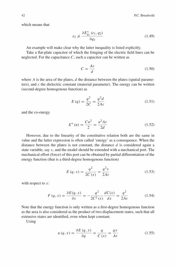
42 P.C. Breedveld
which means that
e2 �=∂E∗q1
(e1, q2)
∂q2(1.49)
An example will make clear why the latter inequality is listed explicitly.Take a flat-plate capacitor of which the fringing of the electric field lines can be
neglected. For the capacitance C , such a capacitor can be written as
C = Aε
d(1.50)
where A is the area of the plates, d the distance between the plates (spatial parame-ters), and ε the dielectric constant (material parameter). The energy can be written(second-degree homogenous function) as
E (q) = q2
2C= q2d
2Aε(1.51)
and the co-energy
E∗ (u) = Cu2
2= u2 Aε
2d(1.52)
However, due to the linearity of the constitutive relation both are the same invalue and the latter expression is often called ‘energy’ as a consequence. When thedistance between the plates is not constant, the distance d is considered again astate variable, say x , and the model should be extended with a mechanical port. Themechanical effort (force) of this port can be obtained by partial differentiation of theenergy function (that is a third-degree homogenous function)
E (q, x) = q2
2C (x)= q2x
2Aε(1.53)
with respect to x :
F (q, x) = ∂E(q, x)
∂x= − q2
2C2 (x)
dC(x)
dx= q2
2Aε(1.54)
Note that the energy function is only written as a first-degree homogenous functionas the area is also considered as the product of two displacement states, such that allextensive states are identified, even when kept constant.
Using
u (q, x) = ∂E (q, x)
∂q= q
C (x)= qx
Aε(1.55)
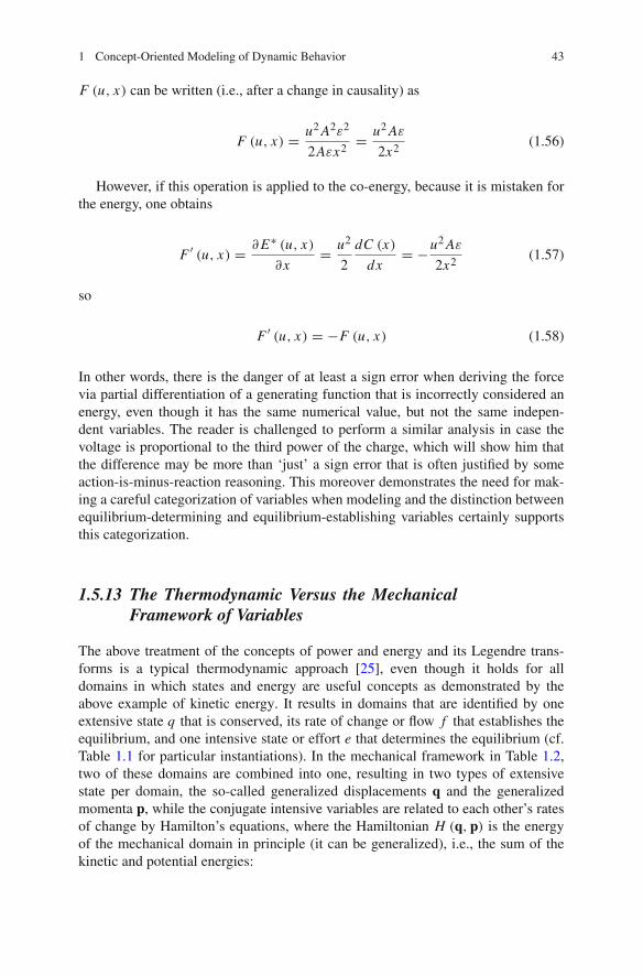
1 Concept-Oriented Modeling of Dynamic Behavior 43
F (u, x) can be written (i.e., after a change in causality) as
F (u, x) = u2 A2ε2
2Aεx2= u2 Aε
2x2(1.56)
However, if this operation is applied to the co-energy, because it is mistaken forthe energy, one obtains
F ′ (u, x) = ∂E∗ (u, x)
∂x= u2
2
dC (x)
dx= −u2 Aε
2x2(1.57)
so
F ′ (u, x) = −F (u, x) (1.58)
In other words, there is the danger of at least a sign error when deriving the forcevia partial differentiation of a generating function that is incorrectly considered anenergy, even though it has the same numerical value, but not the same indepen-dent variables. The reader is challenged to perform a similar analysis in case thevoltage is proportional to the third power of the charge, which will show him thatthe difference may be more than ‘just’ a sign error that is often justified by someaction-is-minus-reaction reasoning. This moreover demonstrates the need for mak-ing a careful categorization of variables when modeling and the distinction betweenequilibrium-determining and equilibrium-establishing variables certainly supportsthis categorization.
1.5.13 The Thermodynamic Versus the MechanicalFramework of Variables
The above treatment of the concepts of power and energy and its Legendre trans-forms is a typical thermodynamic approach [25], even though it holds for alldomains in which states and energy are useful concepts as demonstrated by theabove example of kinetic energy. It results in domains that are identified by oneextensive state q that is conserved, its rate of change or flow f that establishes theequilibrium, and one intensive state or effort e that determines the equilibrium (cf.Table 1.1 for particular instantiations). In the mechanical framework in Table 1.2,two of these domains are combined into one, resulting in two types of extensivestate per domain, the so-called generalized displacements q and the generalizedmomenta p, while the conjugate intensive variables are related to each other’s ratesof change by Hamilton’s equations, where the Hamiltonian H (q,p) is the energyof the mechanical domain in principle (it can be generalized), i.e., the sum of thekinetic and potential energies:

44 P.C. Breedveld
∂H (q,p)∂pi
= d
dtqi = vi
∂H (q,p)∂qi
= − d
dtpi = −Fi
(1.59)
or
∂H (q,p)∂ (q,p)
=[
0 −I
I 0
][q
p
]
=[
0 −I
I 0
][v
F
]
= J−1
[v
F
]
(1.60)
or, in non-preferred causality
[v
F
]
= J∂H (q,p)∂ (q,p)
(1.61)
where I is a unit matrix and J a so-called symplectic matrix or Poisson structurematrix. Note that the so-called external forces can be simply added to this format, butthe most important conclusion is that when the generalized forces F and generalizedvelocities v are used to describe the physical domains in a generalized mechanicalsense, the asymmetry between these variables is lost, as both can be equilibriumestablishing and equilibrium determining, which makes the use of these conceptsduring modeling harder to use and interpret. However, given the large body of lit-erature that is available on all aspects of this approach an extended mathematicalframework, inspired by a bond graph approach, was coined as ‘port-Hamiltonianapproach’ [26].
Another, even more important drawback of generalization of the mechanicalframework is the fact that the displacement variable that can be used to describestorage of potential energy has the same nature as the variables needed to describethe spatial configuration. In many cases the same variable describes configuration aswell as energy storage. This dual role of the displacement variable has brought manyto believe that force and displacement should be considered to be the conjugatepair of variables for the mechanical domain, which leads to all sorts of confusinganalogies. However, it is easy to see that the initial length of a spring between twomasses does not influence its dynamic properties for linear motions: only the springconstant and the masses determine the natural frequency of this system. However,in case of planar or spatial motion or even linear motion with contact behavior like abouncing ball, the changing configuration modulates the energy transfer and in thosecases the configuration variable will influence the dynamics, but in a fundamentallydifferent manner than an energy state. This is why it is fruitful to distinguish between(potential) energy states (displacements) and configuration states (positions), even ifthe variable turns out to be the same mathematical state. Before the time of symbolicprocessing, reduction of the states to the minimal set of independent states largelysupported the analysis. Using modern computer tools, dependent states can either

1 Concept-Oriented Modeling of Dynamic Behavior 45
be eliminated symbolically or solved numerically afterwards without bothering theuser, even though the user should carefully inspect the results in both cases.
The close relationship between configuration states and energy states createsa preference for configuration-related variables in a model description, i.e., oftengeneralized momenta are replaced by generalized velocities in the relations, whichis rather straightforward in case the linearity of Newton’s law is assumed, whichalways holds in classical mechanics. However, this means that a Legendre transformis performed on the true energy function, the Hamiltonian H
H (q,p) = T (q,p)+ V (q) (1.62)
resulting in the Lagrangian L
L (q, q) = qt p− H (q,p) == T (q,p)+ T ∗ (q, q)− (T (q,p)+ V (q)) == T (q,p)+ T ∗ (q, q)− T (q,p)− V (q) == T ∗ (q, q)− V (q)
(1.63)
in other words, the Lagrangian is the difference between kinetic co-energy T ∗ (q, q)and potential energy V (q), where the position dependence of the kinetic (co-)energyis the result of the coordinate transformation into generalized coordinates.
1.5.14 Energy States Versus Configuration States
As the first use of bond graph concepts was highly related to the mechanical domainand heavily influenced by already existing mathematical modeling approaches formechanical systems, the distinction between energy states and configuration stateswas usually not made and two types of state variables were distinguished, general-ized displacement (q-type state stored via a C-type storage port) and generalizedmomentum (p-type state stored via an I-type storage port). As a consequence,the asymmetry between effort and flow was lost as this approach combines twodomains and treats them as one (refer to thermal inertance paper and thesis). In thetwo-domain approach the generalized potential domain has a generalized force-typeeffort and a generalized velocity-type flow (rate of change of generalized displace-ment, while the generalized kinetic domain has a generalized velocity-type effortand a generalized force-type flow (rate of change of momentum). In bond graphterminology it is easy to see that a unit gyrator expresses that in an inertial framethe net effort of the potential domain is equal to the flow of the kinetic domain,while the effort of the kinetic domain determines the rate of change of displace-ment (flow) in the potential domain. Similarly, if one assumes quasi-stationary, i.e.,non-radiating, electrical circuits, Maxwell’s equations that couple the magnetic andelectric domains can be reduced to a relation that equates the rate of change offlux (linkage) (i.e., the magnetic flow) with a voltage (i.e., the electric effort) and a

46 P.C. Breedveld
current (i.e., the electric flow) with a magnetomotive force (i.e., the magnetic effort).In these specific cases (inertial frame and quasi-stationary networks) the interdo-main relations reduce to identities that are expressed in a bond graph by a unitgyrator called ‘symplectic gyrator’ (SGY). As dualizing, i.e., interchanging the rolesof effort and flow, the graph at one side of the SGY eliminates the SGY, the numberof variables is reduced, and the roles of effort and flow have become symmetric,i.e., the distinction between equilibrium determining and equilibrium establishingcannot be made anymore. This has caused endless discussions about whether a forceis analogous to a voltage or to a current, while the above discussion shows that thisis just a matter of which side of the SGY is dualized in the sense that the roles ofefforts and flows are interchanged. However, given the fact that the energy state ofthe potential domain (displacement) is similar to and often coincides with a config-uration state which is of importance for all domains, it is to be expected that mostof the modeling concepts in the model are part of the potential domain, such thatit is to be expected that dualization of the kinetic domain is more straightforward.Something similar holds for electrical circuits: The only conceptual connection tothe magnetic domain is the ideal coil (inductor), while the rest of the circuit modelis part of the electrical domain. In that case it is also more straightforward to dualizethe magnetic storage port into an I-type port.
Due to the dual role of the displacement variable, it is possible to eliminate thepotential energy by choosing another description of the configuration space. Forinstance, Einstein showed in his general theory of relativity in 1915 that as a math-ematical result, it is possible to eliminate potential energy by such a transformationof the space–time that gravity is reduced to a property (curvature) of space–time.
During the modeling process, where one is not yet interested in the mathemati-cally minimal form of a model, but in a form that allows straightforward interpreta-tion in terms of physical concepts, it is wise to represent the two roles of the positionvariable separated, even if they merge mathematically into one variable when themodel is prepared for analysis or simulation.
The confusion that configuration information may cause when not kept separatefrom other concepts also applies to topological representations. Graphs like circuitdiagrams or bond graphs are often interpreted as spatial relations or even with spatialparameters like an area.
Earlier we discussed that assigning more meaning to certain model representa-tions than they actually have leads to all sorts of confusions, similar to Lewin’sincorrect interpretation of his own experiment, which is an example of confus-ing topological information with spatial information. Although Willems [3] doesrecognize the basic principle of a bond graph that models of physical systems consistof subsystems that are related by bilateral signal flows, these confusions also makehim reject bond graphs when he writes, emphasized by a separate frame at page 66of his paper:
(1) ‘The requirement that the product of effort and flow must be power is sometimesnot natural, for example, in thermal interconnections.’

1 Concept-Oriented Modeling of Dynamic Behavior 47
(2) ‘In connecting terminals of mechanical systems, bond graph modeling equatesvelocities, and sets the sum of the forces equal to zero. In reality one ought toequate positions, not velocities. Equating velocities instead of positions leads toincomplete models.’
(3) ‘Interconnections are made by means of terminals, while energy is transferredthrough ports. Ports involve many terminals simultaneously. The interconnec-tion of two electrical wires involves equating two terminal potentials and puttingthe sum of two terminal currents to zero. The product of effort, namely, theelectrical potential, and flow, namely, the electrical current, for an electricalconnection has the dimension of power, but it is not power. Power involvespotential differences, while the interconnection constraint involves the termi-nal potentials themselves. It is not possible to interpret these interconnectionconstraints as equating the power on both sides of the interconnection point.’
(4) ‘In many interconnections, it is unnecessary to have to worry about conservationof energy.’
In particular points (2) and (3) refer to the earlier mentioned confusion, but wewill extensively comment on all of Willems’ arguments, because they represent thebeliefs of many and lead to erroneous conclusions, not only about bond graphs butabout modeling in general. It should be noted that Willems refers to classical bondgraphs based on the mechanical framework of variables with two types of storageand velocity being a flow-type variable as discussed before.
Ad (1) Any self-respecting thermodynamic textbook will explain that the amountof stored heat is not a state as it does not satisfy the criterion that its cyclic integralequals zero, such that a heat flow is not a rate of change of state. If a model isconstrained to the thermal domain, heat or thermal energy is only a function ofthe stored entropy and can serve as a state in that particular case only. In that casealso pseudo-bond graphs can be used to represent such models, so the constraintthat the two conjugated variables of a bond should always be power conjugated isnot as hard as Willems suggests. Furthermore, he writes in his main text that theuse of entropy flow ‘seems artificial.’ He probably means that for many students ofthermodynamics the concept of an entropy flow is counterintuitive, yet it is a well-accepted concept in physics, which is absolutely necessary to describe the dynamicinteraction of the thermal domain with other domains like the mechanical domainas the well-known treatment of an ideal Carnot cycle demonstrates [25].
Ad (2) The statement ‘In reality one ought to equate positions, not velocities’shows that he does not make a distinction between configuration states (positions)and energy states (displacements). The only difference between a constraint atthe displacement level and a constraint at the velocity level is an initial condi-tion, for instance, the initial distance between two masses connected by a spring.However, the dynamic behavior is not influenced by this initial condition. Theonly argument to use (additional) constraints at the position level can be thatnumerical integration generates errors that may lead to a change in the contri-bution of the initial condition, which means that, due to numerical inaccuracies,the masses in the example drift apart or closer together while they are oscillating.

48 P.C. Breedveld
However, adding such a constraint is a numerical issue and not part of the con-ceptual model. The easiest way to see this is to make a similar statement aboutthe electric charge in an electric circuit: While simulating the behavior of an elec-tric circuit containing capacitors the total charge balance may be distorted due tonumerical errors. Apart from the fact that nobody seems to care about this, prob-ably because charge is much less ‘visible’ than configuration and charge cannotmodulate the interconnection structure, a constraint at the charge level can still beadded in the numerical solution procedure to improve accuracy. However, positionvariables also describe the configuration state and often one variable plays bothroles. For planar and spatial mechanisms the configuration variables can influ-ence the dynamics via modulation when the coordinate transformations requiredto describe the interconnection structure are position dependent. These coordi-nate transformations are represented in bond graphs by a modulated multiporttransformer [27]. In conclusion one may state that the constraints in the junctionstructure of the bond graph are energetic constraints at the velocity level, whilethe configuration constraints are dealt with at the signal level, both for modulat-ing the MTFs in the generalized junction structure and for finding potential rela-tions between initial conditions, e.g., two springs connected between the samemasses.
Ad (3) He writes: ‘Interconnections are made by means of terminals, whileenergy is transferred through ports.’
Here the actual configuration (‘interconnection’) is mixed up with conceptualrelationships.
He continues: ‘Ports involve many terminals simultaneously.’First of all, it should be clear about which domain we talk: in a mechanical sys-
tem a terminal may correspond to a port, while mostly two electrical terminals arerequired to create an electrical port. However, Willems fails to give examples ofports consisting of more than two terminals and unless he is referring to multiports,which would be confusing, more than two terminals per port are not possible, unlessone uses a rather uncommon definition of a terminal.
He then writes: ‘The interconnection of two electrical wires involves equatingtwo terminal potentials and putting the sum of two terminal currents to zero. Theproduct of effort, namely, the electrical potential, and flow, namely, the electricalcurrent, for an electrical connection has the dimension of power, but it is not power.Power involves potential differences, while the interconnection constraints involvesthe terminal potentials themselves. It is not possible to interpret these interconnec-tion constraints as equating the power on both sides of the interconnection point.’
The conceptual error in this argument lies in the use of the concept ‘wire.’Willems uses this as something for which a current is a meaningful concept as soonas one terminal of the wire is connected to the terminal of another wire. However, acurrent is a ‘through-variable,’ which means that a connection to a second terminalat the other side, commonly with a component in between, is required to make theconcept of current meaningful. Not only the current requires two terminals, alsothe voltage, as it is a relative concept and always measured with respect to somereference (‘ground’). This means that all potentials are in fact potential differences,

1 Concept-Oriented Modeling of Dynamic Behavior 49
while Willems only considers potential differences with respect to potentials thatare not the ground potential.
This makes clear that any two electrical terminals, also if one is grounded andnot represented as such, form a port. However, in many treatments of electricalcircuits the logical order is reversed: First, a distinction is made between potentialand potential differences. Next a relation between the potential differences and thepotentials is derived via the incidence matrix and only then it is recognized that oneof the rows (balance equations) refers to a reference node (ground) which should beomitted from the incidence matrix to obtain the so-called reduced incidence matrix.This culture may have led Willems to drawing this conclusion.
In his main text (page 68) Willems even writes about this:‘In electrical circuits, energy is not transmitted along terminals but rather through
ports. On the other hand, in modeling and interconnection, terminals matter, notports.’
He then explains the difference in his Fig. 11 where it becomes clear that heassumes that connecting two terminals with each other suffices for electrical inter-connection, which is not the case: A current can only flow after a second connectionthat creates a loop.
This shows that he does not appreciate the difference between a drawing of somephysical components soldered together (= ‘mechanical’ connection) which does notlead to a device that has any electrical meaning as no current can flow and an elec-trical circuit diagram in which connections may coincide with physical connections(soldering points), but may as well be conceptual.
Ad (4) Any textbook on (classical) physics will explain that if one models thedynamics of physical systems, one should always consider the conservation ofenergy, the most general principle of physics. However, the power involved in someof the relations in a system may be negligible with respect to the power of otherrelations and this is probably what Willems tries to say; however, he formulates it insuch a way that it becomes an implicit modeling assumption that power is negligible.A bond graph represents such a modeling decision by ‘bond activation,’ turning thebond into a signal for one of the conjugate variables while assuming the other tobe negligible. This shows that Willems, like many others, including those who usebond graphs, has not taken the effort of studying what a bond graph representationreally is about, but that he has considered explanatory text in a particular context tobe a unique and generic definition.
Another highly related confusion is the concept of a ‘memristor’ introducedby Chua [28]. When one studies Chua’s paper from a bond graph perspective itbecomes clear that he refers to what in a bond graph would be optimally repre-sented by a state-modulated transformer for which Chua coined the name ‘mem-ristor’ due to the seemingly missing link between the q-type and p-type variablesin the mechanical frame work of variables (Table 1.2). Note that the more generalthermodynamical framework would never suggest this relation. Not much attentionhas been paid to this concept until recently, where some researchers came acrossan interesting phenomenon that can be best described as a state-modulated resistor,where the state can be set to different values without much ‘leakage,’ in other words:

50 P.C. Breedveld
a resistor with a memory. They immediately saw the latter as a reason to rewrite theirequations into a form that more or less resembles Chua’s equations and next claimedthat the memristor was finally found [29], which again demonstrates the commonconfusion between physical components and ideal conceptual elements.
1.5.15 Conservation and Continuity Within a Domain
As each conserved state determines a domain, additional connection constraints canbe found for various port types. For instance, a bond connected to one side of a0-junction may be connected to a C-type storage port or a source port, as theseports do not violate the balance equation. However, in principle, one should be morecareful when connecting an I-type, R-type, TF-type, or GY-type port, because theseports cannot ‘absorb’ the conserved state related to the flow. However, all domainswith relative equilibrium-determining variables have a non-displayed balance forthe reference node (this balance equation is dependent on the balance equations forthe rest of the network and corresponds to the row that is omitted in an incidencematrix to turn it into a reduced incidence matrix of an electrical circuit, for exam-ple). This additional balance compensates for this flow, such that it is still possibleto connect these ports without violating the balance equation. Note that the I-typeport in principle is a connection to a GY-type port that connects to the storage inanother domain. Some domains have absolute equilibrium-determining variables,like temperature and pressure, but since in most cases it is not practical to choosethe absolute zero point as a reference, usually another reference state is chosen, suchthat these variables are treated as differences with respect to an arbitrary referenceand an additional balance too.
Further note that labeling energy with a domain is only possible in case of one-port storage as multiport storage means that other domains have access to the storedenergy, such that it does not belong to one domain when stored. As we have seenbefore, one-port storage is the result of neglecting all ports of other states becausethey are considered constant, but it does not exist in principle, because a first-degreehomogenous energy function of a one-port storage element would lead to a zero-order homogenous relation between effort and state, which would mean that theeffort would be a constant. So, also in principle, it is not appropriate to assign adomain to energy, as it can be reached via more than one port, unless the flows ofall other ports are kept zero.
1.6 Conclusion
The warm bed of dynamic models in the form of a set of differential equations ora block diagram in an a priori fixed causality has been replaced by the cold floorof port-based modeling concepts with causal preferences and constraints. Hope-fully the new revelation caused by this disturbing experience is the insight that the
1 Concept-Oriented Modeling of Dynamic Behavior 51
causality assignment procedure gives the modeler immediate feedback on his mod-eling decisions, because the causal consequences of interconnection constraints canbe seen immediately in the context of the physical concepts instead of being theresult of an abstract analysis that hides the relation to the physics.
Another key issue of this contribution is to make clear that three kinds of struc-tures, viz., configuration structure (spatial structure), physical structure, and con-ceptual structure are often mixed up during the modeling of dynamic behavior ofphysical systems. The earlier mentioned lecture where Lewin gives an area (spatial)interpretation to a conceptual (topological) representation and incorrectly assignssimilarity of points in a conceptual representation to points in a spatial representa-tion is an example of such a mix-up. Willems’ problems to understand bond graphsare an example of a confusion of physical structure (‘soldering’ physical compo-nents together not resulting in a configuration that has a meaning in an electricalsense) and conceptual structure that shows the relations between ideal elements thatrepresent dominant behaviors of these components in a particular context, viz., acircuit in that allows electrical phenomena, viz., currents. Again it is emphasizedthat much attention was paid to these cases, not for the sake of having a special-ized scientific discussion with opponents, but because these examples clarify howeasy it is to become the victim of the conceptual trap of forgetting about implicitassumptions.
The common criticism that bond graphs are not well defined has been counteredby showing that their key properties can be defined up to a certain level, but that,like any other language, dialects remain possible and it is up to the user to define theexact meaning of specific symbols.
References
1. Beeren W., Roessink M. (eds) (1998) Sporen van wetenschap in kunst/Traces of Science inArt, 155pp., ISBN 90-6984-224-6.
2. Paynter H.M. (1961) Analysis and Design of Engineering Systems. MIT Press, Cambridge,MA.
3. Willems J.C. (2007) The behavioral approach to open and interconnected systems. IEEE Con-trol Syst. Mag. Dec:46–99.
4. Bondy J.A., Murty U.S.R. (1976) Graph Theory with Applications. North-Holland, Oxford,ISBN 0-444-19451-7.
5. Breedveld P.C. (1982b) Proposition for an unambiguous vector bond graph notation. Trans.ASME, J. Dyn. Syst. Meas. Control 104(3):267–270.
6. Breedveld P.C. (1986) A definition of the multibond graph language. In Complex and Dis-tributed Systems: Analysis, Simulation and Control, Tzafestas S., Borne P. (eds) Vol. 4 of‘IMACS Transactions on Scientific Computing’. North-Holland, Amsterdam, pp. 69–72.
7. Breedveld P.C. (1982a) Thermodynamic bond graphs and the problem of thermal inertance. J.Franklin Inst. 314(1):15–40.
8. Karnopp D.C., Rosenberg R.C. (1968) Analysis and simulation of multiport systems. MITPress, Cambridge, MA.
9. Hogan N.J., Fasse, E.D. (1988) Conservation principles and bond graph junction structures.Proc. ASME 1988 WAM. DSC 8:9–14.

52 P.C. Breedveld
10. Paynter H.M., Busch-Vishniac I.J. (1988) Wave-scattering approaches to conservation andcausality. J. Franklin Inst. 325(3):295–313.
11. Breedveld P.C. (1985) Multibond graph elements in physical systems theory. J. Franklin Inst.319(1/2):1–36.
12. Blundell A.J. (1982) Bond Graphs for Modelling Engineering Systems. Ellis Horwood, Chich-ester and Halsted Press, New York, NY, 151p.
13. Thoma J. (1975) Introduction to Bond Graphs and Their Applications. Pergamon Press,Oxford.
14. Breedveld P.C. (2009) Port-based modeling of dynamic systems. Chapter 1 and appendix Aand B2. In Modeling and Control of Complex Physical Systems – The Port-HamiltonianApproach, Stramigioli S., Macchelli A., Duindam V., Bruyninckx H. (eds). Springer, Berlin,pp. 1–52, 97–311, 323–328.
15. Breedveld P.C. (1984). Decomposition of multiport elements in a revised multibond graphnotation. J. Franklin Inst. 318(4):253–273.
16. Breedveld P.C. (1995) Exhaustive decompositions of linear two-ports. Proceedings of SCS1995 International Conference on Bond Graph Modeling and Simulation (ICBGM’95), SCSSimulation Series 27(1):11–16, Jan 15–18, Las Vegas, Cellier F.E., Granda J.J. (eds). ISBN1-56555-037-4.
17. Dijk J. van, Breedveld P.C. (1991a) Simulation of system models containing zero-order causalpaths – part I: Classification of zero-order causal paths. J. Franklin Inst. 328(5/6):959–979.
18. Breedveld P.C. (2007) Port-based modeling of engineering systems in terms of bond graphs.In Handbook of Dynamic System Modeling, Fishwick P.A. (ed). Chapman & Hall, London,pp. 26.1–26.29, ISBN 1-58488-565-3.
19. Dijk J. van, Breedveld P.C. (1991b) Simulation of system models containing zero-order causalpaths – part II: Numerical implications of class-1 zero-order causal paths. J. Franklin Inst.328(5/6):981–1004.
20. Feynman R, Leighton R, Sands M. (1989) The Feynman Lectures on Physics. 3 volumes 1964,1966, Addison-Wesley, Reading, Mass, ISBN 0-201-50064-7.
21. Zill D.G. (2005) A First Course in Differential Equations. 9th edition. Brooks/Cole, Belmont,CA, ISBN-13: 978-0-495-10824, Lib. of Congress number: 2008924906.
22. Wellstead P.E. (1979) Introduction to physical systems modeling. Academic, London. ISBN:0-12-744380-0.
23. Timoshenko S. (1976) Strength of Materials: Elementary Theory and Problems. Vol. 1 ofStrength of Materials, 3rd edition, R.E. Krieger, Huntington, NY (First ed. D. Van NostrandCompany, inc., 1940).
24. Allen R.R. (1981) Dynamics of mechanisms and machine systems in accelerating referenceframes. Trans. ASME J. Dyn. Syst. Meas. Control 103(4):395–403.
25. Callen H.B. (1960) Thermodynamics. Wiley, New York, NY.26. Maschke B.M., van der Schaft A.J., Breedveld P.C. (1995) An intrinsic Hamiltonian formu-
lation of the dynamics of LC-circuits. Trans. IEEE Circuits Syst. I Fundam. Theory Appl.42(2):73–82.
27. Karnopp D.C. (1978) The energetic structure of multibody dynamic systems. J. Franklin Inst.306(2):165–181.
28. Chua L.O. (1971) Memristor-the missing circuit element. IEEE Trans. Circuit Theory CT-18(5):507–519.
29. Strukov D.B., Snider G.S., Stewart D.R., Williams, R.S. (2008) The missing memristor found.Nature 453. doi:10.1038/nature06932.


