Page 1
Documento de Trabajo Nro. 208
Marzo, 2017
ISSN 1853-0168
www.cedlas.econo.unlp.edu.ar
Boosting Tourism’s Contribution to Growth and Development: Analysis of Evidence
Onil Banerjee, Martín Cicowiez y Emily J. Morris
Page 2
-1-
Boosting Tourism’s Contribution to Growth and Development: Analysis of Evidence
Onil Banerjeea, Martín Cicowiez
b and Emily J. Morris
c
a Corresponding author
Inter-American Development Bank
Environment, Rural Development, Environment and Disaster Risk Management Division
1300 New York Avenue N.W.
Washington, D.C., 20577, USA
+1 202 942 8128
[email protected]
b Universidad Nacional de la Plata
Facultad de Ciencias Económicas
Calle 6 entre 47 y 48, 3er piso, oficina 312
1900
La Plata, Argentina
c Inter-American Development Bank
Country Department Central America, Mexico, Panama and the Dominican Republic
1300 New York Avenue N.W.
Washington, D.C., 20577, USA
Page 3
-2-
Abstract
In this study we develop an evidence-based tool to help to guide policy and investment
choices, to maximize developmental returns from tourism. Specifically, we develop a
tourism-extended social accounting matrix and computable general equilibrium and
microsimulation models customized for tourism investment analysis. To demonstrate the
approach, we develop these data structures for Belize, at both national and regional levels.
The framework developed herein can be used to quantify the direct and indirect, and short-
and long-run impacts of tourism investments. Anticipating application of the approach to
tourism investment analysis in the Central American Region, we provide a stock take of the
availability of data to develop a similar suite of models for other countries in the region.
Keywords: ex-ante economic impact analysis; tourism investment analysis; tourism
development; economy-wide model; microsimulation model; Belize; Central America.
Page 4
-3-
Table of Contents
1.0. Introduction ......................................................................................................................... 4
2.0. Methods and Data ............................................................................................................... 5
2.1. The Computable General Equilibrium Model ...................................................... 6 2.2. Social Accounting Matrix ................................................................................... 10 2.3. Non-SAM Data ................................................................................................... 18
2.4. Microsimulation Model and Data ....................................................................... 19 3.0. Scenario Design ................................................................................................................ 22
4.0. Results ............................................................................................................................... 24
4.1. Macro Results ..................................................................................................... 24 4.2. Sectoral Results .................................................................................................. 27
4.3. Poverty Results ................................................................................................... 29 4.4. Sensitivity Analysis ............................................................................................ 29
5.0. Assessment of Data Availability in CID Region .............................................................. 31
6.0. Concluding Remarks ......................................................................................................... 33
References ................................................................................................................................ 36
Appendix A: RCGE Model Mathematical Statement .............................................................. 38
Appendix B: Technical Note on the Construction of the RSAM for Belize Cayo District ..... 56
Appendix C: Processing of HES 2008-2009 ........................................................................... 68
Page 5
-4-
1.0. Introduction
Belize boasts diverse natural resources as well as rich cultural heritage, which provide a
range of attractions for tourists. For the past 15 years tourism has grown to be an important
sector of Belize’s economy, with around 340,000 overnight visitors in 2015 and a further
960,000 cruise arrivals. The World Travel and Tourism Council (WTTC) estimates that the
industry’s direct contribution to GDP grew from 8.5 percent in 2000 to 13.9 percent in 2016
(WTTC, 2016). As noted by the government (GOB, 2012 and 2015), tourism has strong
potential for further expansion in Belize, and is therefore a priority sector for Belize’s
strategy for economic development, as it is for the IDB’s Country Strategy for Belize (IDB,
2013).
The tourism supply chain involves a wide range of sectors of the society and economy. The
industry’s contribution to growth, poverty reduction and long term development depends
upon complex economic, social, environmental and institutional linkages, spillovers and
externalities. To maximize the positive effects and minimize the negative, policy-makers
need to understand what types of tourism, and kinds of policies, are associated with the most
beneficial results, and how to stimulate the types of private sector innovation and investment
(domestic and international, large and small) that foster them.
In this study we develop an evidence-based tool to help to guide policy and investment
choices, to maximize developmental returns from tourism. Specifically, we develop tourism-
extended social accounting matrices and computable general equilibrium and
microsimulation models for Belize, at both national and regional levels.
The computable general equilibrium (CGE) model of Belize’s national economy (and of its
six regions) presented here is ready to be applied. Hence, where estimates related to specific
tourism-related investments are available, the model can be used to quantify the direct and
indirect, and short- and long-run impacts. For instance, it could be used to estimate the
impacts of building a port for cruise ships and/or improving the road to Caracol, a world
renowned Mayan archeological site. To that end, the analyst implementing the model would
need access to: (i) investment projections and (ii) an estimate of the expected impact on gross
tourist arrivals and/or tourist spending.
This report is structured as follows. Section 2 describes the model and its dataset. Section 3
describes the baseline and a set of scenarios to identify the impact of investment policy
decisions related to the development of the tourism sector of Belize under different tourism
Page 6
-5-
demand assumptions. Specifically, we focus on Belize’s Cayo District as an illustrative case
study. Section 4 presents the model results. The study closes with a stock take of the available
data to implement our modeling approach more broadly, both in Belize and in the other
Central American countries. A detailed description of the model and data is provided in the
Appendix to the study.
2.0. Methods and Data
The tourism industry is far from being an isolated sector: indeed, it is an important
component of many sectors, ranging from the hotels and restaurants sector where it is
dominant, to food and beverages and transport, where its influence is also strong. Similarly,
investments in diverse sectors contribute to the development of tourism, from infrastructure
development, the provision of basic public services such as water and sanitation, and capacity
building in the services sector, to institutional strengthening in terms of tourism-sector
governance. Thus, in order to assess the impact of any of the many types of policy
interventions, investments and external shocks that might affect the tourism sector, a
framework that considers all economic sectors and their inter-linkages is essential (see, for
example, Dwyer (2015)). The CGE model provides a systematic method for predicting both
the direction and approximate magnitudes of impacts of policies and external shocks on
different agents. In this study, a national/regional, tourism-extended recursive dynamic
computable CGE model for Belize is developed and applied.
The modeling framework developed here can be used in different contexts, such as other
countries in the CID region. In fact, our model was developed as a “standard” (flexible
structural) model. Thus, there is a complete separation between model code and database.
Specifically, the model comprises the following files: (a) a generic set of model files in
GAMS (General Algebraic Modeling System)1, and (b) application-specific files in Excel for
data and simulations. Thus, anything that is not specific to an application dataset for the
particular country or regional case appears in the model code. Finally, note that the model
code is written and customized to capture whatever data is available in each case.
The modelling framework is not only designed to be applicable to different countries or
regions, but also to be sufficiently flexible to allow customizable versions. Users can
therefore select from: a national or regional model version; a static or dynamic model
1 https://www.gams.com/
Page 7
-6-
version; flexible (dis)aggregation (e.g., sectors and/or factors) options; alternatives specified
for selected assumptions; the application of a special treatment for the (domestic and foreign)
tourism sector; macro closures2; rules for government receipts and spending; rules for non-
government payments; presence/absence of (endogenous) unemployment; and various other
features.
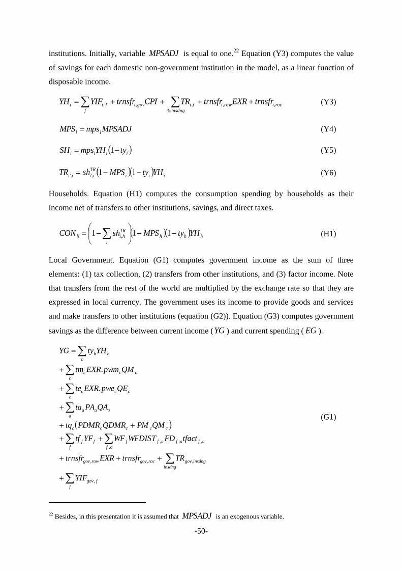
2.1. The Computable General Equilibrium Model
In essence, the CGE model combines a relatively standard recursive dynamic computable
general equilibrium model (see, for example, Lofgren et al. (2002) and Robinson (1989))
with additional equations and variables that, depending on data availability, can single out:
(a) the domestic and foreign tourism demand, (b) different modalities of tourism supply and
demand, and (c) the impact of public capital investment in infrastructure on sectoral
productivity. Moreover, the regional (that is, sub-national) variant of the model can handle (a)
trade between the modeled region and the rest of the country and the rest of the world, and
(b) local and central government operations in the modeled region (i.e., tax collection and
current and capital spending)3. Thus, compared to other CGE models, the one developed here
provides a combination of policy-relevant features for the study of tourism investment or
policy counterfactual scenarios in a national/regional economy.
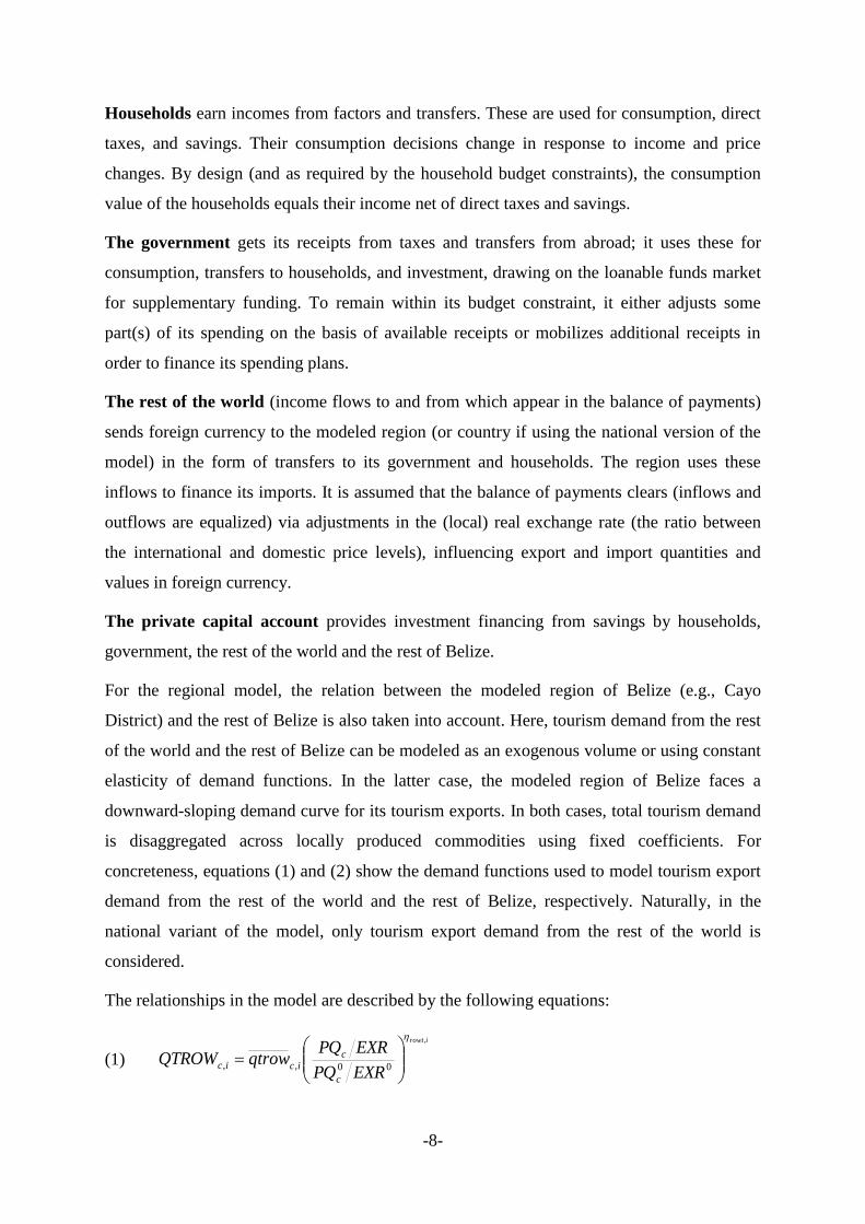
The regional variant of the model is similar to the national variant, but with additional
elements to capture transactions between the modeled regional economy and the rest of the
country. Figure 1 depicts, for each simulation period, the circular flow of income within the
regional (subnational) economy and between this regional economy and the rest of the
country and the rest of the world.
For the national economy as a whole, the major building blocks of our CGE model may be
divided into: activities (producers of commodities), markets for commodities (goods and
services); markets for factors (labor, land and capital stock) and private capital, and four
2 In a CGE model, the macro closure refers to the rules on the basis of which a market (quantity demanded =
quantity supplied) or a macro balance (income = expenditure) clears. In any application, the model macro
closure comprises three elements: (a) government (adjustment of one or more receipt or spending items), (b)
balance of payments (adjustment of the real exchange rate -- more common -- or of a non-trade foreign
exchange flow), and (c) savings-investment balance (investment clears -- investment is savings driven -- or one
or more savings flows adjust -- savings is investment driven).
3 In fact, our starting point for model development was our previous work as published in Banerjee et al. (2015)
and Banerjee et al. (2016). In addition, a multi-regional variant of the model has been developed. Again, the
application of the multi-regional model depends on the availability of regional data such as regional
employment and/or GDP by sector. In practice, such data is required to build a multi-regional dataset, starting
from a national dataset.
Page 8
-7-
institutions: households, government, the rest of the world, and tourists (both domestic and
foreign). As shown, foreign and domestic tourism are sources of income for the modeled
region. Specifically, foreign tourism is a source of foreign exchange. In any application (and
database) of our CGE model, most blocks in Figure 1 are disaggregated – the disaggregation
in the Belize Cayo District regional CGE (RCGE) application is shown in Table 2 below.
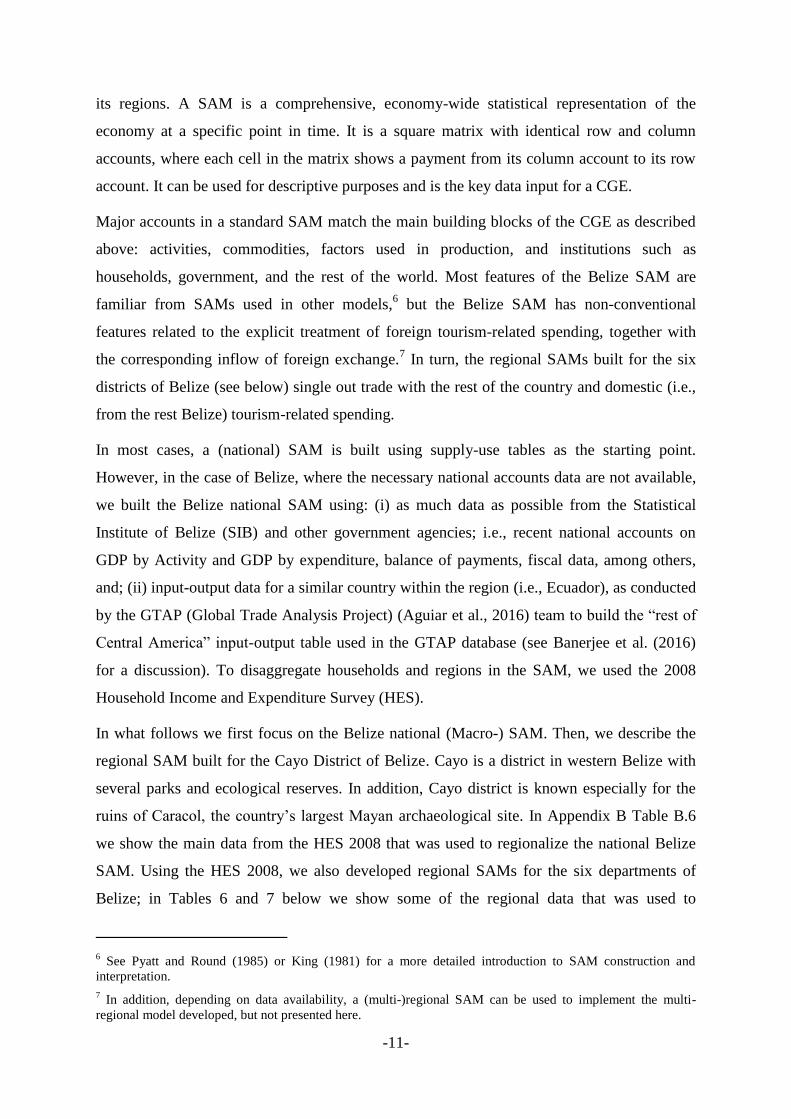
Figure 1. Circular income flow in the RCGE; within-period module
Source: Author’s own elaboration.
In any single year, the (regional) CGE model has the structure summarized in the above
figure.
Activities produce, selling their output at home or abroad (i.e., the rest of Belize and/or the
rest of the world), and use their revenues to cover their costs (of intermediate inputs, factor
hiring and taxes) and provide a return to investors. Their decisions to pursue particular
activities with certain levels of factor use are driven by profit maximization. The shares of
output that are exported and sold domestically depend on the relative prices of the output in
world, national, and domestic markets. For any exported commodity, exporters face either (a)
export prices (here we refer to free on board prices) that are exogenously determined, in
which case export demand is infinitely price-elastic; or (b) price-sensitive export demands
(defined by constant-elasticity functions) with the free on board export prices linked to
domestic conditions (e.g., the costs of production) and the real exchange rate.
Factor Markets
Activities
Households
CommodityMarkets
Rest of World + Restof Country
Government
PrivateCapital
Account
domestic wages and rents
fact
or d
eman
d
foreign + RoC wages and rents
domestic demand
exports
imports
interm input demand
priv
ate
cons
umpt
ion
gov cons and inv
indirect taxes
private savings
tran
sfer
s
tran
sfer
s
tran
sfer
s
dire
ctta
xes
fore
ign
+ Ro
Csa
ving
s
governmentdeficit
private investment
RoW + RoCTourists
Page 9
-8-
Households earn incomes from factors and transfers. These are used for consumption, direct
taxes, and savings. Their consumption decisions change in response to income and price
changes. By design (and as required by the household budget constraints), the consumption
value of the households equals their income net of direct taxes and savings.
The government gets its receipts from taxes and transfers from abroad; it uses these for
consumption, transfers to households, and investment, drawing on the loanable funds market
for supplementary funding. To remain within its budget constraint, it either adjusts some
part(s) of its spending on the basis of available receipts or mobilizes additional receipts in
order to finance its spending plans.
The rest of the world (income flows to and from which appear in the balance of payments)
sends foreign currency to the modeled region (or country if using the national version of the
model) in the form of transfers to its government and households. The region uses these
inflows to finance its imports. It is assumed that the balance of payments clears (inflows and
outflows are equalized) via adjustments in the (local) real exchange rate (the ratio between
the international and domestic price levels), influencing export and import quantities and
values in foreign currency.
The private capital account provides investment financing from savings by households,
government, the rest of the world and the rest of Belize.
For the regional model, the relation between the modeled region of Belize (e.g., Cayo
District) and the rest of Belize is also taken into account. Here, tourism demand from the rest
of the world and the rest of Belize can be modeled as an exogenous volume or using constant
elasticity of demand functions. In the latter case, the modeled region of Belize faces a
downward-sloping demand curve for its tourism exports. In both cases, total tourism demand
is disaggregated across locally produced commodities using fixed coefficients. For
concreteness, equations (1) and (2) show the demand functions used to model tourism export
demand from the rest of the world and the rest of Belize, respectively. Naturally, in the
national variant of the model, only tourism export demand from the rest of the world is
considered.
The relationships in the model are described by the following equations:
(1)
irowt
EXRPQ
EXRPQqtrowQTROW
c
cicic
,
00,,
Page 10
-9-
(2)
iroct
CPIPQ
CPIPQqtrocQTROC
c
cicic
,
00,,
where
c = tourism-related commodities such as hotels and restaurants
i = tourism demand modalities such as tourist and business visitors
icQTROW , = Rest of the World (RoW) tourism type i demand quantity of commodity c
icQTROC , = Rest of Country (RoC) tourism type i demand quantity of commodity c
cPQ = composite commodity price for c
CPI = consumer price index
EXR = exchange rate
icqtroc
, = baseline RoC tourism type i demand quantity of commodity c
icqtroc
, = baseline RoW tourism type i demand quantity of commodity c
iroct , = constant price elasticity of RoC tourism demand (< 0)
irow, = constant price elasticity of RoW tourism demand (< 0)
As shown, we use constant elasticity of demand functions to model tourism export demand
from RoW and RoC. In addition, note that, within domestic and foreign tourism demand, the
model allows for the identification of one or more tourism demand modalities (i.e., see index
i in equations (1) and (2)).4 In equation (1), foreign tourists’ demand is a function of local
(tourism-related) prices relative to the exchange rate EXR. In equation (2), national tourists’
demand is a function of local (tourism-related) prices relative to the consumer price index
CPI. Note that although tourists from the rest of Belize do not need to change currencies, a
real exchange rate exists between any specific region of Belize that is being modeled and the
rest of the country, defined as the ratio between regionally tradable and non-tradable
commodities such as housing.
On the supply side, the modeling of alternative tourism modalities – for example, all-
inclusive beach resorts, boutique hotels, eco-lodges – is straightforward. Provided data is
4 For example, index i in equation (1) can refer to tourists from different countries.
Page 11
-10-
available, the model can consider different cost structures for the different tourism modalities
on the supply side.
In domestic commodity markets, flexible prices ensure balance between demand and supply.
Import prices in most cases would be exogenous, but the assumptions of the model can be
adjusted for cases where their prices are endogenous (for example, in the case of the regional
model, where a large increase in imports from a specific region could push up the price). The
share of imports in the national market is determined by their prices relative to domestic
prices.
In factor markets, demand curves are downward-sloping reflecting the responses of
production activities to changes in factor prices. In the case of labor, unemployment is
endogenous. For each labor type, the model assumes an inverse relationship between the real
wage and the unemployment rate5 (Blanchflower and Oswald, 1994 and 2005). The model
allows for the input of assumptions for labor mobility in response to wage differentials
between Belize and outside, and (in the regional version) between one region and another
within Belize. For non-labor factors, the supply curves are vertical in any single year: that is,
their quantity is fixed, but price adjusts according to the level of demand.
In our CGE, national income growth over time is largely endogenous. The economy grows
due to the expansion of capacity determined by net fixed capital formation (investment minus
depreciation) and the availability of labor (determined by exogenously imposed projections),
as well as improvements in total factor productivity (TFP) which have both endogenous and
exogenous components. Endogenous determinants of TFP include the levels of government
capital stock (public goods) and economic openness. The accumulation of private and
government capital is through investment financed by local and external savings. Increased
private capital is allocated across sectors according to their relative profitability. Once
installed, capital becomes sector-specific and can only by adjusted through exogenously-
determined depreciation and the attraction of new investments.
2.2. Social Accounting Matrix
The basic accounting structure and much of the underlying data required to implement our
Belize RCGE model is derived from a Social Accounting Matrix (SAM) for Belize or one of
5 In this case, the unemployment elasticity of the real wage is assumed to be -0.1, which is consistent with
estimates derived from the literature. That is, a 1% increase in the unemployment rate is assumed to reduce
wages by 0.1%.
Page 12
-11-
its regions. A SAM is a comprehensive, economy-wide statistical representation of the
economy at a specific point in time. It is a square matrix with identical row and column
accounts, where each cell in the matrix shows a payment from its column account to its row
account. It can be used for descriptive purposes and is the key data input for a CGE.
Major accounts in a standard SAM match the main building blocks of the CGE as described
above: activities, commodities, factors used in production, and institutions such as
households, government, and the rest of the world. Most features of the Belize SAM are
familiar from SAMs used in other models,6 but the Belize SAM has non-conventional
features related to the explicit treatment of foreign tourism-related spending, together with
the corresponding inflow of foreign exchange.7 In turn, the regional SAMs built for the six
districts of Belize (see below) single out trade with the rest of the country and domestic (i.e.,
from the rest Belize) tourism-related spending.
In most cases, a (national) SAM is built using supply-use tables as the starting point.
However, in the case of Belize, where the necessary national accounts data are not available,
we built the Belize national SAM using: (i) as much data as possible from the Statistical
Institute of Belize (SIB) and other government agencies; i.e., recent national accounts on
GDP by Activity and GDP by expenditure, balance of payments, fiscal data, among others,
and; (ii) input-output data for a similar country within the region (i.e., Ecuador), as conducted
by the GTAP (Global Trade Analysis Project) (Aguiar et al., 2016) team to build the “rest of
Central America” input-output table used in the GTAP database (see Banerjee et al. (2016)
for a discussion). To disaggregate households and regions in the SAM, we used the 2008
Household Income and Expenditure Survey (HES).
In what follows we first focus on the Belize national (Macro-) SAM. Then, we describe the
regional SAM built for the Cayo District of Belize. Cayo is a district in western Belize with
several parks and ecological reserves. In addition, Cayo district is known especially for the
ruins of Caracol, the country’s largest Mayan archaeological site. In Appendix B Table B.6
we show the main data from the HES 2008 that was used to regionalize the national Belize
SAM. Using the HES 2008, we also developed regional SAMs for the six departments of
Belize; in Tables 6 and 7 below we show some of the regional data that was used to
6 See Pyatt and Round (1985) or King (1981) for a more detailed introduction to SAM construction and
interpretation.
7 In addition, depending on data availability, a (multi-)regional SAM can be used to implement the multi-
regional model developed, but not presented here.
Page 13
-12-
disaggregate the national SAM. In Appendix B we describe the steps that were followed to
build the national and regional SAMs for Belize. A similar procedure can be followed to
build (national and regional) SAMs for other countries in the region.
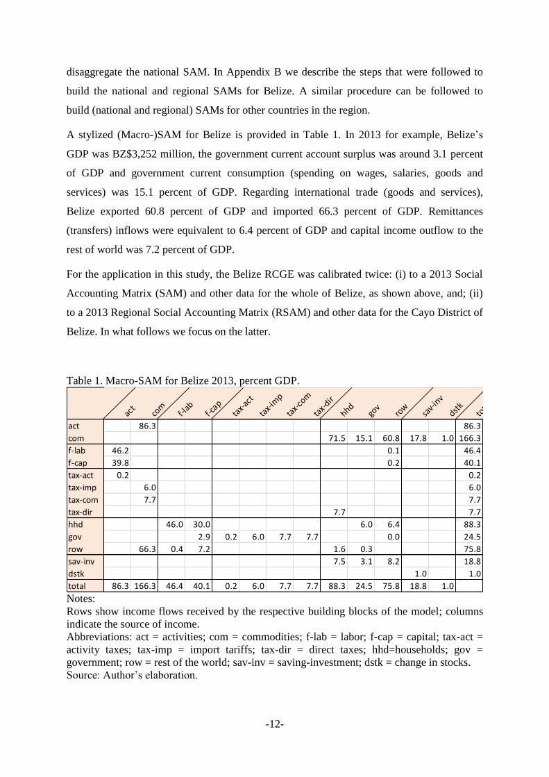
A stylized (Macro-)SAM for Belize is provided in Table 1. In 2013 for example, Belize’s
GDP was BZ$3,252 million, the government current account surplus was around 3.1 percent
of GDP and government current consumption (spending on wages, salaries, goods and
services) was 15.1 percent of GDP. Regarding international trade (goods and services),
Belize exported 60.8 percent of GDP and imported 66.3 percent of GDP. Remittances
(transfers) inflows were equivalent to 6.4 percent of GDP and capital income outflow to the
rest of world was 7.2 percent of GDP.
For the application in this study, the Belize RCGE was calibrated twice: (i) to a 2013 Social
Accounting Matrix (SAM) and other data for the whole of Belize, as shown above, and; (ii)
to a 2013 Regional Social Accounting Matrix (RSAM) and other data for the Cayo District of
Belize. In what follows we focus on the latter.
Table 1. Macro-SAM for Belize 2013, percent GDP.
Notes:
Rows show income flows received by the respective building blocks of the model; columns
indicate the source of income.
Abbreviations: act = activities; com = commodities; f-lab = labor; f-cap = capital; tax-act =
activity taxes; tax-imp = import tariffs; tax-dir = direct taxes; hhd=households; gov =
government; row = rest of the world; sav-inv = saving-investment; dstk = change in stocks.
Source: Author’s elaboration.
act
com
f-lab
f-cap
tax-
act
tax-
imp
tax-
com
tax-
dir
hhdgo
vro
wsa
v-in
v
dstk
tota
l
act 86.3 86.3
com 71.5 15.1 60.8 17.8 1.0 166.3
f-lab 46.2 0.1 46.4
f-cap 39.8 0.2 40.1
tax-act 0.2 0.2
tax-imp 6.0 6.0
tax-com 7.7 7.7
tax-dir 7.7 7.7
hhd 46.0 30.0 6.0 6.4 88.3
gov 2.9 0.2 6.0 7.7 7.7 0.0 24.5
row 66.3 0.4 7.2 1.6 0.3 75.8
sav-inv 7.5 3.1 8.2 18.8
dstk 1.0 1.0
total 86.3 166.3 46.4 40.1 0.2 6.0 7.7 7.7 88.3 24.5 75.8 18.8 1.0
Page 14
-13-
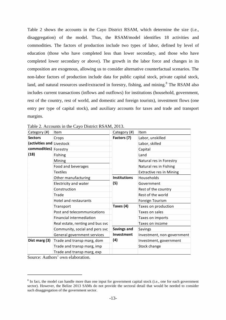
Table 2 shows the accounts in the Cayo District RSAM, which determine the size (i.e.,
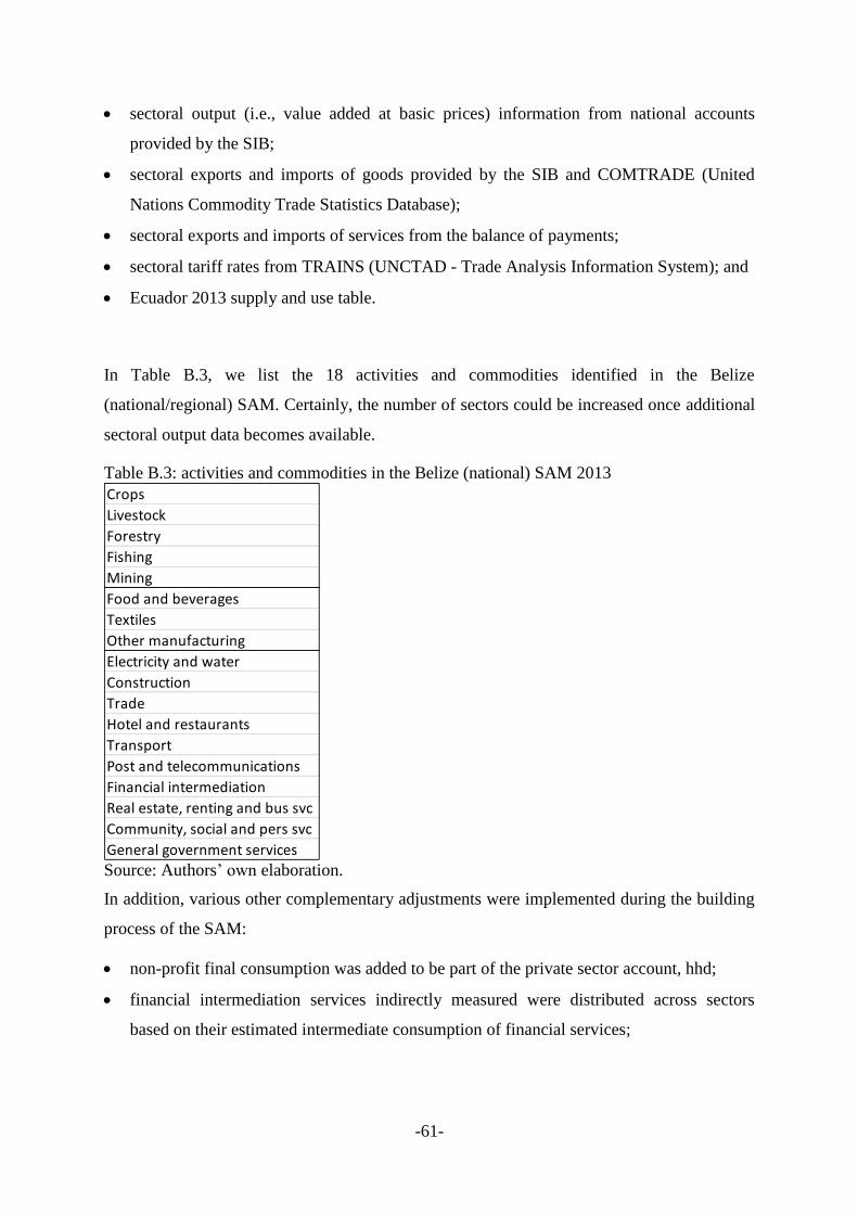
disaggregation) of the model. Thus, the RSAM/model identifies 18 activities and
commodities. The factors of production include two types of labor, defined by level of
education (those who have completed less than lower secondary, and those who have
completed lower secondary or above). The growth in the labor force and changes in its
composition are exogenous, allowing us to consider alternative counterfactual scenarios. The
non-labor factors of production include data for public capital stock, private capital stock,
land, and natural resources used/extracted in forestry, fishing, and mining.8 The RSAM also
includes current transactions (inflows and outflows) for institutions (household, government,
rest of the country, rest of world, and domestic and foreign tourists), investment flows (one
entry per type of capital stock), and auxiliary accounts for taxes and trade and transport
margins.
Table 2. Accounts in the Cayo District RSAM, 2013.
Source: Authors’ own elaboration.
8 In fact, the model can handle more than one input for government capital stock (i.e., one for each government
sector). However, the Belize 2013 SAMs do not provide the sectoral detail that would be needed to consider
such disaggregation of the government sector.
Category (#) Item Category (#) Item
Crops Labor, unskilled
Livestock Labor, skilled
Forestry Capital
Fishing Land
Mining Natural res in Forestry
Food and beverages Natural res in Fishing
Textiles Extractive res in Mining
Other manufacturing Households
Electricity and water Government
Construction Rest of the country
Trade Rest of the world
Hotel and restaurants Foreign Tourism
Transport Taxes on production
Post and telecommunications Taxes on sales
Financial intermediation Taxes on imports
Real estate, renting and bus svc Taxes on income
Community, social and pers svc Savings
General government services Investment, non-government
Trade and transp marg, dom Investment, government
Trade and transp marg, imp Stock change
Trade and transp marg, exp
Sectors
(activities and
commodities)
(18)
Taxes (4)
Savings and
Investment
(4)Dist marg (3)
Institutions
(5)
Factors (7)
Page 15
-14-
According to our estimates in the RSAM, the Cayo District’s Gross Regional Product (GRP)
reached BZ$696.7 million in 2013 (see Table 3), equivalent to 21.5 percent of the national
Gross Domestic Product (GDP). In 2013, local and central government current consumption
in Cayo District was 16.4 percent of gross regional product (GRP), and total fixed capital
formation and remittances from abroad accounted for 19 and 6.9 percent of GRP,
respectively.
Table 3. Gross Regional Product (GRP), Belize Cayo District 2013.
Source: Author’s own calculations based on 2013 Belize Cayo District SAM.
On the basis of RSAM data, Table 4 summarizes the sectoral structure of the Cayo District’s
economy in 2013: sectoral shares in value-added, production, employment, exports and
imports, as well as the split of domestic sectoral supplies between exports and domestic sales,
and domestic sectoral demands between imports and domestic output. In terms of trade with
the rest of Belize, columns (EXP-RoCshr) and (IMP-RoCshr) of Table 4 show the share of
each sector in total exports and imports to/from the rest of the country, respectively. For
instance, while hotels and restaurants represent a significant share of employment (around 5.8
percent), its share of exports is much larger (around 26.4 percent). The 2013 Belize Cayo
District SAM also reports taxes paid by institutions, commodity sales, value added, activities,
and tariffs; total tax revenue reached 22.3 percent of GRP in 2013.
Item mill BZ$ GRP%
Total Demand
Private consumption 531.9 76.3
Fixed investment 132.7 19.0
Stock change -4.7 -0.7
Government consumption 114.4 16.4
Exports to RoW 263.7 37.9
Exports to RoC 162.2 23.3
Tourism demand RoC 0.0 0.0
Tourism demand RoW 154.6 22.2
Total 1,354.9 194.5
Total Supply
GRP at market prices 696.7 100.0
Imports from RoW 479.5 68.8
Imports from RoC 178.7 25.7
Total 1,354.9 194.5
GRP = gross regional product
Page 16
-15-
Table 4. Sectoral structure of GRP, Belize Cayo District 2013, percent share.
Source: Authors’ own elaboration.
Sector VAshr PRDshr EMPshr EXPshr
EXP-
OUTshr IMPshr
IMP-
DEMshr
Crops 7.4 4.8 8.5 9.8 65.0 1.6 25.2
Livestock 2.1 5.1 2.7 0.0 0.1 0.2 1.3
Forestry 0.7 0.4 2.3 0.1 7.4 0.0 2.2
Fishing 2.7 2.4 1.6 0.1 1.1 0.0 0.0
Mining 0.8 5.6 1.0 17.8 99.9 0.3 14.1
Food and beverages 6.8 10.4 3.9 32.9 100.0 11.6 84.5
Textiles 0.0 0.0 1.0 0.0 5.8 1.9 85.1
Other manufacturing 7.2 10.6 6.2 1.7 5.0 67.5 76.9
Electricity and water 4.4 6.7 1.4 0.0 0.0 0.0 0.0
Construction 3.9 3.2 9.8 0.0 0.0 0.0 0.0
Trade 17.2 12.2 16.6 0.0 0.0 0.0 0.0
Hotel and restaurants 4.3 8.4 5.8 26.4 99.9 2.9 10.7
Transport 3.5 3.4 4.3 1.7 15.8 6.9 35.2
Post and telecommunications 3.4 3.2 0.5 0.4 4.4 0.6 3.0
Financial intermediation 2.7 2.9 0.7 0.1 1.5 2.4 12.8
Real estate, renting and bus svc 7.1 4.4 4.8 3.4 24.0 2.8 29.1
Community, social and pers svc 8.2 5.2 19.8 5.6 34.3 1.2 7.2
General government services 17.7 11.2 9.2 0.0 0.0 0.0 0.0
Total 100.0 100.0 100.0 100.0 31.6 100.0 31.2
Page 17
-16-
Table 4 continued. Sectoral structure of GRP, Belize Cayo District 2013, percent share.
Glossary: VAshr = value-added share (%); PRDshr = production share (%); EMPshr = share
in total employment (%); EXPshr = sector share in total exports (%); EXP-OUTshr = exports
as share in sector output (%); IMPshr = sector share in total imports (%); IMP-DEMshr =
imports as share of domestic demand (%); EXP-RoCshr = sector share in total exports to RoC
(%); EXP-RoC-OUTshr = exports to RoC as share in sector output (%); IMP-RoCshr =
sector share in total imports from RoC (%); IMP-RoC-DEMshr = imports from RoC as share
of domestic demand (%). Source: Authors’ calculations based on 2013 Belize Cayo District
SAM and employment data.
Table 5 shows the factor shares in total sectoral value added. For example, the table shows
that agriculture (Crops and Livestock) is relatively intensive in the use of unskilled labor and
land; this information will be useful to analyze the results from the Belize Cayo District
RCGE simulations. In turn, General government services and Financial intermediation
sectors are relatively intensive in the use of skilled labor.
Sector
EXP-
RoCshr
EXP-RoC-
OUTshr
IMP-
RoCshr
IMP-RoC-
DEMshr
Crops 0.1 0.2 0.8 4.0
Livestock 1.3 3.1 11.8 23.6
Forestry 0.9 31.2 0.1 4.2
Fishing 0.6 3.4 5.9 25.4
Mining 0.0 0.0 5.0 80.4
Food and beverages 4.6 5.5 0.4 1.0
Textiles 0.0 29.7 0.0 0.0
Other manufacturing 32.9 38.0 3.0 1.2
Electricity and water 5.9 10.7 0.5 1.2
Construction 3.8 14.6 0.3 1.5
Trade 0.1 0.1 0.5 0.6
Hotel and restaurants 0.3 0.4 2.8 3.8
Transport 1.0 3.6 9.0 17.3
Post and telecommunications 3.6 14.0 32.9 59.3
Financial intermediation 2.5 10.5 22.7 45.5
Real estate, renting and bus svc 10.8 29.8 1.0 3.8
Community, social and pers svc 0.0 0.1 0.4 0.9
General government services 31.5 34.5 2.9 5.0
Total 100.0 12.3 100.0 31.2
Page 18
-17-
Table 5. Sectoral factor intensity, Belize Cayo District 2013, percent sectoral value added at
factor cost.
Source: Author’s calculations based on 2013 Belize SAM and employment data.
In Tables 6 and 7 we present regional data computed from the HES 2008. As previously
discussed, this data was used to estimate regional social accounting matrices for the six
departments of Belize.
Sector
Labor,
unskilled
Labor,
skilledCapital Nat Res Total
Crops 52.3 5.7 19.8 22.2 100.0
Livestock 58.0 6.3 16.8 18.9 100.0
Forestry 28.8 22.1 44.3 4.8 100.0
Fishing 45.9 3.9 20.1 30.1 100.0
Mining 6.4 1.8 46.7 45.1 100.0
Food and beverages 16.0 22.4 61.6 0.0 100.0
Textiles 38.2 21.8 40.0 0.0 100.0
Other manufacturing 23.5 22.6 53.9 0.0 100.0
Electricity and water 8.3 35.4 56.3 0.0 100.0
Construction 46.0 15.4 38.6 0.0 100.0
Trade 34.7 38.5 26.8 0.0 100.0
Hotel and restaurants 27.5 31.5 41.0 0.0 100.0
Transport 17.0 36.5 46.6 0.0 100.0
Post and telecommunications 5.3 49.7 45.0 0.0 100.0
Financial intermediation 7.7 61.5 30.8 0.0 100.0
Real estate, renting and bus svc 5.6 36.3 58.2 0.0 100.0
Community, social and pers svc 21.3 60.9 17.8 0.0 100.0
General government services 15.6 63.3 21.1 0.0 100.0
Total 24.5 37.5 34.8 3.2 100.0
Page 19
-18-
Table 6. Household per capita expenditures by district, Belize 2008, BZ$
Source: Author’s calculations based on HES 2008.
Table 7. Poverty headcount ratio by district, Belize 2008, 2.5 and 4 PPP US dollars-a-day
poverty lines.
Source: Author’s calculations based on HES 2008.
In order to single out alternative supply modalities of tourism, estimates such as those shown
in Table 8 for the Nicaragua municipalities of Granada would be needed. Of course, matching
estimates from the demand side would also be needed. In the case of Belize (and Cayo
District), we do not have access to such data. Thus, our RSAM considers a single tourism
supply and demand modality. In addition, and again due to the lack of data, we cannot
distinguish between domestic and foreign tourists.
Table 8. Cost structure, supply modalities for the Municipality of Granada in 2013, percent.
Source: Authors’ own elaboration.
2.3. Non-SAM Data
In addition to the SAM, our Belize RCGE model requires: (a) base year estimates for capital
stocks, and sectoral employment levels and unemployment estimates for the different labor
Department Mean Median S.d.
Corozal 3,654 2,694 3,907
Orange Walk 4,895 3,367 6,822
Belize 7,183 4,041 12,537
Cayo 5,258 2,764 10,607
Stann Creek 4,902 2,322 13,007
Toledo 2,274 1,413 3,566
Total 5,284 2,905 10,190
Department 2.5 USD 4 USD
Corozal 33.3 52.2
Orange Walk 26.5 44.7
Belize 23.3 34.5
Cayo 36.7 53.9
Stann Creek 47.0 62.5
Toledo 66.2 76.8
Total 34.7 49.6
ItemHotel, 1
Star
Hotel, 2
Stars
Hotel, 3
Stars
Hotel, 4
Stars
Hotel, 5
Stars
Restauran
ts and
Intermediate consumption, goods 23.1 14.9 22.7 11.8 15.8 25.6
Intermediate consumption, services 10.0 23.6 13.8 18.1 13.6 8.0
Wages 31.4 20.8 38.8 23.0 41.7 17.9
Capital and other (*) 35.4 40.8 24.8 47.1 28.9 48.5
Total 100 100 100 100 100 100
(*) includes tax payments
Page 20
-19-
types; (b) a set of elasticities (for production, consumption and trade); (c) population
projections by household group (i.e., rural and urban); and (d) a baseline projection for
growth in GDP at factor cost (see below). In order to estimate sectoral employment we
combined population data from the United Nations with estimates for the unemployment rate
computed from the 2013 labor force survey. In turn, elasticities were given values based on
the available evidence for comparable countries. Specifically, the following values were
used: (a) the elasticity of substitution among factors is in the 0.2–1.15 range, relatively low
for primary sectors and relatively high for manufactures and services (see Aguiar et al.
(2016)); (b) the wage curve has an unemployment-elasticity of -0.1 (see Blanchflower and
Oswald (2005)); and (c) based on Sadoulet and de Janvry (1995), trade elasticities are in the
0.5-2 range. Finally, note that in Section 4 we conduct a systematic sensitivity analysis of our
CGE model results with respect to the values of these parameters.
2.4. Microsimulation Model and Data
As discussed, CGE models are effective in capturing macro and meso (i.e., for 30-35 sectors)
responses to shocks such as an improvement in the terms of trade. However, the standard
configuration of a CGE model is not well suited for analysis of questions related to poverty
and income inequality. This is due to the fact that most CGE models use a representative
household (RH) formulation where all households in an economy are aggregated into one or a
few households to represent household and consumer behavior. The main limitation of the
RH formulation is that intra-household income distribution does not respond to shocks
introduced into the model.
Consequently, in order to provide greater resolution with regard to household-level impacts,
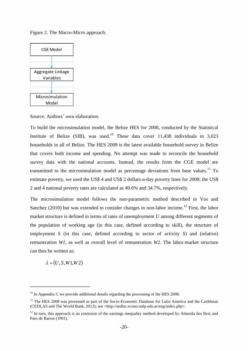
we generate results in terms of poverty and inequality at the micro level by linking the CGE
model with a microsimulation model (see Figure 2.2). The two models interact in a sequential
“top-down” fashion (i.e., without feedback): the CGE communicates with the
microsimulation model by generating a vector of (real) wages9, aggregate employment
variables such as labor demand by sector and the unemployment rate, and non-labor income.
The functioning of the labor market thus plays an important role, and the CGE model
determines the changes in employment by factor type and sector, and changes in factor and
product prices that are then used for the microsimulations.
9 The real wage is defined in terms of the CPI; see the RCGE model mathematical statement in the Appendix A.
Page 21
-20-
Figure 2. The Macro-Micro approach.
Source: Authors’ own elaboration.
To build the microsimulation model, the Belize HES for 2008, conducted by the Statistical
Institute of Belize (SIB), was used.10
These data cover 11,438 individuals in 3,023
households in all of Belize. The HES 2008 is the latest available household survey in Belize
that covers both income and spending. No attempt was made to reconcile the household
survey data with the national accounts. Instead, the results from the CGE model are
transmitted to the microsimulation model as percentage deviations from base values.11
To
estimate poverty, we used the US$ 4 and US$ 2 dollars-a-day poverty lines for 2008; the US$
2 and 4 national poverty rates are calculated as 49.6% and 34.7%, respectively.
The microsimulation model follows the non-parametric method described in Vos and
Sanchez (2010) but was extended to consider changes in non-labor income.12
First, the labor
market structure is defined in terms of rates of unemployment U among different segments of
the population of working age (in this case, defined according to skill), the structure of
employment S (in this case, defined according to sector of activity S) and (relative)
remuneration W1, as well as overall level of remuneration W2. The labor-market structure
can thus be written as:
2,1,, WWSU
10
In Appendix C we provide additional details regarding the processing of the HES 2008.
11 The HES 2008 was processed as part of the Socio-Economic Database for Latin America and the Caribbean
(CEDLAS and The World Bank, 2012); see <http://sedlac.econo.unlp.edu.ar/eng/index.php>.
12 In turn, this approach is an extension of the earnings inequality method developed by Almeida dos Reis and
Paes de Barros (1991).
CGE Model
Aggregate Linkage
Variables
Microsimulation
Model
Page 22
-21-
The effect of altering each of its four parameters on poverty and inequality can then be
analyzed by simulating counterfactual individual earnings and family incomes. Briefly, the
model selects at random (with multiple repetitions) from the corresponding labor groups the
individuals who will change labor market status (i.e., employment/unemployment and sector)
and assigns wages to new workers according to parameters for the average groups. Then, the
new wage and employment levels for each individual result in new household per capita
incomes that are then used to determine the new poverty and income distribution results.
Analytically, we can write
ii Xfyl ,
where
iyl = individual labor income
iX = individual characteristics; e.g., skill level
In each counterfactual scenario, labor market conditions might change and in turn affect the
individual labor income; i.e.,
ii Xfyl ,**
where * refers to the simulated labor market structure parameters.
The labor market variables and procedures that link the CGE model with the
microsimulations are as follows. This “unemployment effect” is simulated by changing the
labor status of the active population in the HES 2008 sample, based on the results from the
CGE model. For instance, if according to the CGE simulations, unemployment decreases at
the same time that employment increases for skilled workers in sector A, the microsimulation
model “hires” randomly from the HES 2008 sample among the unemployed skilled workers.
As explained above, individual incomes for the newly employed are assigned based on their
characteristics (e.g., educational level) by looking at similar individuals that were originally
employed. If the CGE simulations indicate a decrease in employment for a specific labor
category and sector, the microsimulation program “fires” the equivalent percentage from the
type of labor and sector, and the counterfactual income for those newly unemployed is zero.
The “sectoral structure effect” is simulated by changing the sectoral composition of
employment. For those individuals that move from one sector to another, we simulate a
counterfactual labor income based on their characteristics and on their new sector of
Page 23
-22-
employment, again by looking at individuals that were originally employed in the sector of
destination.
To model the change in relative wages, the wage level for a given labor category (e.g., skilled
workers in sector A) are adjusted according to the changes from the CGE simulations but
keeping the aggregate average wage for the economy constant. The impact of the change in
the aggregate average wage for the economy is simulated by changing all labor incomes in all
sectors by the same proportion, based on the changes from the CGE simulations. Next, all the
previous steps are repeated several times and averaged.
For non-labor incomes, government transfers and remittances from abroad are proportionally
scaled up or down using changes taken from the CGE model. The final step in the
microsimulation model is to adjust the micro data such that the percentage change in the
household per capita income matches the change in the level of household per capita income
– for each representative household in the CGE simulations. Thus, this residual effect
implicitly accounts for changes in all items not previously considered (i.e., non-labor and
non-transfer incomes) such as natural resource and capital rents.
Finally, we should note that our CGE model can only solve for the relative prices and the real
variables of the economy. Thus, in order to anchor the absolute price level, a normalization
rule has been applied. Specifically, the consumer price index (CPI) is chosen as the
numéraire, so all changes in nominal prices and incomes in simulations are relative to the
weighted unit price of households’ initial consumption bundle (i.e., a fixed CPI). The model
is also homogenous of degree zero in prices. In macro terminology, the model displays
neutrality of money.
3.0. Scenario Design
This section presents the simulations and analyzes the results. To illustrate the use of the
model and dataset we have developed, the following four scenarios were simulated and
analyzed:
Base: the baseline or reference scenario is the “business-as-usual” scenario;
Page 24
-23-
Invest: 25 percent increase during 2016-2020 in government investment in tourism-
related infrastructure; financed with transfers from the rest of the country. These transfers
implicitly represent transfers from the central government13
.
Dem: 3.5 percent yearly increase in foreign tourism demand and arrivals during 2016-
2020; afterwards (i.e., 2021-2030) foreign tourism demand is around 20% higher than in
the baseline; and
Combi: scenarios invest and dem combined.
In the base, we assume that average past trends will continue from 2013 to 2030. In fact, in
the absence of better projections, it is assumed that Belize’s Cayo District is on a balanced
growth path, which means that real or volume variables, including tourism demand, grow at
the same rate while relative prices do not change.
The three non-base simulations only deviate from the base beginning in 2016 to 2030.
Certainly, the non-base shocks we are considering are arbitrary, but are designed to illustrate
the mechanics of the model. In fact, is likely that any tourism-related scenario will contain
some of the elements present in this set of simulations.
Figure 3. Definition of scenarios ‘invest’ and ‘dem’, percent deviation from base.
Source: Authors’ elaboration.
13
It should be noted that in this application, no additional government spending on operations and maintenance
of the new capital stock was included. The model does, however, allow for this additional spending to be
included in the simulation.
0
5
10
15
20
25
30
20
13
20
15
20
17
20
19
20
21
20
23
20
25
20
27
20
29
Gov Fixed Investment
0
2
4
6
8
10
12
14
16
18
20
20
13
20
15
20
17
20
19
20
21
20
23
20
25
20
27
20
29
Foreign Tourism Demand
Page 25
-24-
At the macro level, our RCGE, as any other CGE model, requires the specification of the
equilibrating mechanism for three macroeconomic balances. For the non-base scenarios these
are:
(i) The impact on the government fiscal balance is cleared via changes in income tax
rates on households. This assumption ensures that the simulations are budget neutral;
that is, there is no additional domestic and/or foreign financing beyond baseline
values.
(ii) Private investment in the Cayo District follows an exogenously imposed path; given
this path, adjustments in savings from the rest of Belize clear the savings-investment
balance; and
(iii) The real exchange rate adjusts to equilibrate inflows and outflows of foreign
exchange, by influencing export and import quantities. That is, the simulations are
neutral in terms of changes in region net foreign assets. The non-trade-related
payments of the (local) balance of payments (transfers and foreign investment) are
non-clearing, following exogenously imposed paths.
In addition, given the regional character of the model, a mechanism is required to clear the
current account of the balance of payments between the local economy and the rest of the
country. Specifically, it is assumed that the real exchange rate is flexible with respect to the
RoC, with equilibrium achieved through changes in the price of local non-tradable
commodities. In other words, prices for non-tradable commodities are region-specific, while
for tradable commodities the local price is a weighted average of the price of three different
varieties: local, from the RoC, and from the RoW.
4.0. Results
4.1. Macro Results
The base year of the model as presented here is 2013. For the baseline scenario, which serves
as a benchmark for comparisons, we impose an average growth of 2.5 percent, based on
projections from the April 2016 International Monetary Fund World Economic Outlook
(IMF, 2016).14
In addition, due to the assumption of a balanced growth path, the following
assumptions were also imposed: (i) macro aggregates are kept fixed as a share of the gross
14
The exogenous part of total factor productivity growth is adjusted to generate such a growth path. In non-base
scenarios, GRP growth is endogenous.
Page 26
-25-
regional product at base year values; (ii) transfers to/from government/RoC/RoW to
households are also kept fixed as a share of GRP; and (iii) tax rates are fixed over time.
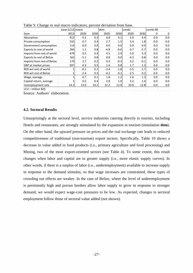
In Table 9 and Figures 4a and 4b, we show key macroeconomic results for the baseline and
other scenarios for the year 2020 (i.e., the year when the simulated tourism-related
infrastructure investment is completed) and 2030. In Table 9, all indicators are for the Cayo
District alone. As the table shows, the increase in government tourism-related investment has,
in the medium- long-run, a positive impact on the activity level (simulation invest). On the
other hand, the inflow of foreign resources -- both from RoC to finance investment and from
RoW due to increased tourist arrivals -- gives rise to slower non-tourism (goods and services)
export growth and faster import growth, both of which were induced by an appreciation of
the regional real exchange rate.15
In turn, the expansion of tourism demand tends to expand
domestic absorption more rapidly than it expands GRP, also causing deterioration in the non-
tourism trade balance (scenario dem). In other words, the increase in “tourism exports” also
generates an appreciation of the real exchange rate that hurts the other tradable (mainly
goods) sectors. Slower export growth here is a function of increasing domestic demand and
prices in Cayo District due to the investment. Where factor supply constraints exist
(labor/capital/land/natural resources), increased domestic prices relative to world prices result
in a reallocation of resources toward domestic production to meet more rapid growth in
domestic demand.
15
Notice that “exports” do not include tourism-related spending made by foreigners. Certainly, the latest
correspond to tourism exports, but the two are treated differently in the model and Table 3.1.
Page 27
-26-
Figure 4a. Change in real private consumption 2015-2030, percent deviation from base.
Figure 4b. Change in real gross regional product 2015-2030, percent deviation from base.
Source: Authors’ own elaboration.
0.0
0.5
1.0
1.5
2.0
2.5
3.0
3.5
4.0
20
15
20
16
20
17
20
18
20
19
20
20
20
21
20
22
20
23
20
24
20
25
20
26
20
27
20
28
20
29
20
30
invest dem combi
-0.5
0.0
0.5
1.0
1.5
2.0
2.5
20
15
20
16
20
17
20
18
20
19
20
20
20
21
20
22
20
23
20
24
20
25
20
26
20
27
20
28
20
29
20
30
invest dem combi
Page 28
-27-
Table 9. Change in real macro indicators, percent deviation from base.
Source: Authors’ elaboration.
4.2. Sectoral Results
Unsurprisingly at the sectoral level, service industries catering directly to tourists, including
Hotels and restaurants, are strongly stimulated by the expansion in tourism (simulation dem).
On the other hand, the upward pressure on prices and the real exchange rate leads to reduced
competitiveness of traditional (non-tourism) export sectors. Specifically, Table 10 shows a
decrease in value added in food products (i.e., primary agriculture and food processing) and
Mining, two of the most export-oriented sectors (see Table 4). To some extent, this result
changes when labor and capital are in greater supply (i.e., more elastic supply curves). In
other words, if there is a surplus of labor (i.e., underemployment) available to increase supply
in response to the demand stimulus, so that wage increases are constrained, these types of
crowding out effects are weaker. In the case of Belize, where the level of underemployment
is persistently high and porous borders allow labor supply to grow in response to stronger
demand, we would expect wage-cost pressures to be low. As expected, changes in sectoral
employment follow those of sectoral value added (not shown).
base (LCU) invest dem combi combi-BE
Item 2013 2020 2030 2020 2030 2020 2030 0 0
Absorption 912 0.2 0.3 4.8 4.1 5.0 4.4 0.0 0.0
Private consumption 532 0.7 0.4 2.7 1.5 3.4 1.8 0.0 0.0
Government consumption 114 0.0 0.0 0.0 0.0 0.0 0.0 0.0 0.0
Exports to rest of world 264 1.1 0.8 -4.8 -6.6 -3.7 -5.7 0.0 0.0
Imports from rest of world 479 0.5 0.4 4.5 2.9 5.0 3.3 0.0 0.0
Exports to rest of Belize 162 -5.1 0.8 0.8 0.0 -4.3 0.8 0.0 0.0
Imports from rest of Belize 179 2.7 0.2 0.4 -0.3 3.2 -0.1 0.0 0.0
GRP at market prices 697 0.3 0.5 1.4 0.8 1.7 1.3 0.0 0.0
RER wrt rest of world 1 -0.1 0.1 -3.4 -1.8 -3.5 -1.7 0.0 0.0
RER wrt rest of Belize 1 -2.4 0.3 -0.2 -0.1 -2.5 0.2 0.0 0.0
Wage, average 1 0.7 0.1 1.8 1.2 2.6 1.3 0.0 0.0
Capital return, average 1 0.5 0.4 2.8 1.0 3.2 1.4 0.0 0.0
Unemployment rate 14.3 13.0 14.2 12.2 12.9 10.9 12.8 0.0 0.0
LCU = million BZ$
Page 29
-28-
Table 10. Change in sectoral real value added, exports, and imports, percent deviation from
base.
Source: Authors’ own elaboration.
base (LCU) invest dem combi
Commodity 2013 2020 2030 2020 2030 2020 2030
Value Added
Crops 44 -0.3 0.7 -2.8 -2.7 -3.3 -2.0
Livestock 12 -1.0 0.2 0.1 -0.5 -0.9 -0.3
Forestry 4 0.9 1.0 0.0 -0.4 0.8 0.6
Fishing 16 -0.8 0.4 -0.3 -1.0 -1.1 -0.6
Mining 5 2.6 1.2 -5.3 -9.3 -2.3 -8.0
Food and beverages 41 0.6 0.8 -4.5 -6.6 -4.0 -5.8
Textiles 0 -1.7 0.9 5.9 4.8 4.1 5.7
Other manufacturing 43 -1.8 0.2 1.4 1.1 -0.5 1.4
Electricity and water 26 -0.6 0.2 0.8 0.5 0.3 0.7
Construction 23 18.4 1.2 0.6 0.3 19.0 1.5
Trade 103 0.4 0.4 1.3 0.6 1.6 1.0
Hotel and restaurants 25 0.0 0.2 15.3 15.8 15.3 15.9
Transport 21 -0.1 0.5 0.5 0.0 0.4 0.5
Post and telecommunications 20 -1.3 0.2 0.5 0.3 -0.8 0.5
Financial intermediation 16 -1.5 0.5 0.2 -0.2 -1.2 0.3
Real estate, renting and bus svc 43 -0.7 0.6 -0.2 -0.5 -0.9 0.1
Community, social and pers svc 49 0.3 0.4 6.0 5.9 6.3 6.3
General government services 106 -2.1 0.4 -0.1 -0.4 -2.2 0.0
Exports
Crops 41 -0.4 0.7 -3.9 -3.1 -4.4 -2.4
Livestock 0 -0.7 0.3 -2.8 -1.9 -3.6 -1.6
Forestry 0 0.1 1.0 -4.2 -2.6 -4.2 -1.6
Fishing 0 -0.1 0.4 -3.3 -2.1 -3.4 -1.6
Mining 74 2.6 1.2 -5.3 -9.3 -2.3 -8.0
Food and beverages 126 0.8 0.8 -4.9 -6.9 -4.2 -6.1
Textiles 0 -1.2 0.7 0.7 2.9 -0.4 3.6
Other manufacturing 3 -0.8 0.1 -1.9 -0.4 -2.7 -0.3
Transport 2 0.4 0.5 -3.2 -1.8 -2.9 -1.3
Post and telecommunications 1 0.1 0.0 -3.9 -2.1 -3.8 -2.0
Financial intermediation 1 -0.3 0.4 -4.0 -2.5 -4.3 -2.1
Real estate, renting and bus svc 14 0.5 0.3 -4.4 -2.8 -4.0 -2.5
Imports
Crops 8 0.0 0.7 1.4 -1.1 1.3 -0.5
Livestock 1 -0.5 0.1 1.8 0.3 1.4 0.4
Forestry 0 6.7 0.7 4.4 2.1 11.4 2.7
Fishing 0 -0.7 0.3 1.6 -0.5 0.9 -0.3
Mining 2 2.7 2.9 -7.5 -17.2 -3.6 -14.3
Food and beverages 56 0.2 0.6 11.6 9.5 11.7 10.0
Textiles 9 0.6 1.1 11.9 6.2 12.5 7.3
Other manufacturing 324 0.7 0.3 2.4 1.3 3.1 1.6
Hotel and restaurants 14 -0.1 0.1 20.8 18.0 20.7 18.2
Transport 33 0.2 0.5 3.6 1.5 3.8 1.9
Post and telecommunications 3 -0.9 0.2 4.4 2.6 3.5 2.8
Financial intermediation 11 -1.1 0.4 3.7 1.8 2.6 2.2
Real estate, renting and bus svc 14 0.1 1.3 7.8 4.3 8.0 5.7
Community, social and pers svc 6 0.2 0.2 10.3 8.1 10.6 8.4
LCU = million BZ$
Page 30
-29-
The model shows how the size of the economic impacts resulting from increased tourism
demand is determined by key factors: factor supply constraints, real effective exchange rate
appreciation, and current government economic policy (Dwyer et al., 2000).
4.3. Poverty Results
In terms of poverty, our results show, for example, that the 2 dollars-a-day poverty headcount
ratio in the Cayo District falls by 0.7 percentage points in the last year of the simulation
period in the combi scenario (Figure 3.3). The main drivers of this result are a decrease in
unemployment, a higher average wage, and an increase in non-labor income. In terms of
inequality, we find a slight increase, driven by the decrease in the unemployment rate
(because those with the very lowest incomes are under-represented among the newly
employed) and the change in the sectoral structure of employment in favor of the services
sector.
Figure 5. Change in poverty, percentage points from base.
Source: Authors’ elaboration.
4.4. Sensitivity Analysis
As usual, the results from the RCGE model are a function of (i) the model structure (e.g.,
functional forms used to model production and consumption decisions, macroeconomic
closure rule, among other elements); (ii) the base year data used for model calibration (i.e.,
the RSAM); and (iii) the values assigned to the model elasticities or, more generally, to the
model’s free parameters.
Certainly, the elasticities used in this study implicitly carry an estimation error, as in any
similar model. Consequently, we have performed a systematic sensitivity analysis of the
results with respect to the value assigned to the model elasticities. Hence, if the conclusions
-1.2 -1 -0.8 -0.6 -0.4 -0.2 0
invest
dem
combi
2020
US$ 2 pov line US$ 4 pov line
-0.8 -0.6 -0.4 -0.2 0
invest
dem
combi
2030
US$ 2 pov line US$ 4 pov line
Page 31
-30-
of the analysis are robust to changes in the set of elasticities used for model calibration, we
will have greater confidence in the results presented above.
In order to perform the systematic sensitivity analysis, it is assumed that each of the model
elasticities is uniformly distributed around the central value used to obtain the results. The
range of variation allowed for each elasticity is +/- 85%; that is, a wide range of variation for
each model elasticity is considered. Then, a variant of the method originally proposed by
Harrison and Vinod (1992) is implemented, which allows for performing a systematic
sensitivity analysis. In short, the aim is to solve the model iteratively with different sets of
elasticities. Thus, a distribution of results is obtained to build confidence intervals for each of
the model results. The steps for implementing the systematic sensitivity analysis are as
follows.
Step 1. In the first step, the distribution (i.e., lower and upper bound) for each of the model
parameter that will be modified as part of the systematic sensitivity analysis is computed:
elasticities of substitution between primary factor of production, trade-related elasticities,
expenditure elasticities, and unemployment elasticities for the wage curves.
Step 2. In the second step, the model is solved repeatedly, each time employing a different set
of elasticities; it is, therefore, a Monte Carlo type of simulation. First, the value for each
model elasticity is randomly selected. Second, the model is calibrated using the selected
elasticities. Third, the same counterfactual scenarios as previously described are conducted.
Then, the preceding steps are repeated several times, 1,000 in this case, with sampling with
replacement for the value assigned to the elasticities.
Table 11 shows the percentage change in private consumption estimated (i) under the central
elasticities, and; (ii) as the average of the 1,000 observations generated by the sensitivity
analysis. For the second case, the upper and lower bounds under the normality assumption
were also computed; notice that all runs from the Monte Carlo experiment receive the same
weight. As can be seen, the results reported above are significant, while estimates presented
in Table 9 are within the confidence intervals reported in Table 11. For example, there is
virtual certainty that the combi scenario has a positive effect on private consumption in the
Cayo District of Belize.
Page 32
-31-
Table 11. Sensitivity analysis; real private consumption percent deviation from base; year
2030; 95% confidence interval under normality assumption
Source: Authors’ own elaboration.
Figure 6 shows non-parametric estimates of the density function for the percentage change in
2030 in private consumption in the combi scenario. Again, the sign of the results (i.e.,
positive) is not changed when model elasticities are allowed to differ in +/- 80% of their
“central” value.
Figure 6. Sensitivity analysis, real private consumption deviation from base in 2030.
Source: Authors’ own elaboration.
5.0. Assessment of Data Availability in CID Region
In this section, we assess the availability of the data required to implement our tourism-
extended CGE model for the countries in IDB’s Country Department for Central America.
Specifically, we discuss the availability and latest year of the following data:
Scenario Central Elast Mean Standard Dev Lower Bound Upper Bound
invest 0.3835 0.3800 0.0303 0.3206 0.4394
dem 1.4596 1.4391 0.0927 1.2575 1.6207
combi 1.8333 1.8100 0.0916 1.6305 1.9895
01
23
4
kde
nsity c
om
bi
1.4 1.6 1.8 2 2.2percentage change
Page 33
-32-
(a) supply and use tables16
,
(b) other national accounts data such as integrated economic accounts and regionally
disaggregated national accounts17
,
(c) tourism satellite account, and
(d) household surveys capturing household income and expenditure.
In Table 12 we summarize the availability of the required data to build national and sub-
national SAMs for the CID countries. Also, we should note that Mexico is the only country in
the region that, as part of its national accounts data, generates a set of regional accounts at the
state level. For the other countries, one would need to combine the national supply-use tables
with regional data typically obtained from a household and/or enterprise survey in order to
estimate a sub-national social accounting matrix. Specifically, in order to build a regional
(i.e., sub-national) SAM, information on regional sectoral employment and/or GDP would be
required. Then, depending on the required level of geographical disaggregation, information
from an existing household survey can be used, as implemented here for the Departments of
Belize and in Banerjee et al. (2015) for the South Department of Haiti.
However, if the aim is to build a local SAM for a city or municipality, it is usually the case
that the regularly conducted household surveys do not contain enough observations at the
local level to build a local SAM. Thus, a special-purpose household and/or enterprise survey
would be required. In addition, conducting surveys to domestic and foreign tourists is
required to single them out in the SAM. Furthermore, note that all countries considered in
Table 12 regularly produce aggregated national accounts data.
16
“The supply and use tables are in the form of matrices that record how supplies of different kinds of goods
and services originate from domestic industries and imports and how those supplies are allocated between
various intermediate or final uses, including exports”. (OECD Glossary of Statistical Terms).
17 “The integrated economic accounts comprise the full set of accounts of institutional sectors and the rest of the
world, together with the accounts for transactions (and other flows) and the accounts for assets and liabilities.”
(OECD Glossary of Statistical Terms).
Page 34
-33-
Table 12. Availability of data required to build a recent (i.e., circa 2014) social accounting
matrix
Source: Author’s own elaboration based on information from the following institutions:
Belize = Statistical Institute of Belize (SIB);
Costa Rica = Banco Central de Costa Rica and Instituto Nacional de Estadística y Censos
(INEC);
Dominican Republic = Banco Central de la República Dominicana and Oficina Nacional
de Estadística (INEC);
El Salvador = Banco Central de Reserva de El Salvador and Dirección General de
Estadística y Censos (DIGESTYC);
Guatemala = Banco de Guatemala and Instituto Nacional de Estadística (INE);
Honduras = Banco Central de Honduras and Instituto Nacional de Estadística (INE);
Mexico = Instituto Nacional de Estadística y Geografía (INEGI);
Nicaragua = Banco Central de Nicaragua (BCN) and Instituto Nacional de Información
de Desarrollo (INIDE); and
Panama = Instituto Nacional de Estadística y Censo (INEC).
Finally, it is noteworthy that not all the information reviewed above is currently publicly
available through the corresponding institutional web pages. For example, Nicaragua and
Costa Rica are currently in the process of publishing their recently updated national accounts
data. However, it is expected that the said data would be made available to conduct economic
analysis by any government agency, even if it is not publicly available yet.
6.0. Concluding Remarks
This framework has the potential to be applied at the national level, where national level
tourism policies and investments are the subject of analysis, or at the regional level as in the
País
Supply and Use
Tables
Integrated
Economic Acc
National Acc
Sectoral Data HHD Survey InstitutionBelize n.a. n.a. 2013 2008 SIB
Costa Rica 2012 2013 2013 2014 BCCR / INEC
Dominican Republic 2010 n.a. 2014 2014 BCRP / ONE
El Salvador 2006 n.a. 2014 2014 BCR / DIGESTYC
Guatemala 2012 2012 2012 2011 BG / INE
Honduras 2013 2013 2013 2014 BCH / INE
Mexico 2008 2008; desag 2014 2014 INEGI
Nicaragua 2010 2010 2010 2014 BCN / INIDE
Panama 2012 2012; total 2014 2015 INEC
Page 35
-34-
Belize illustration in assessing the impacts of a localized investment. The indicators
generated shed light on income and expenditure impacts, employment, poverty, sectoral
output, as well as trade relations.
Where the analyst is concerned with the net present value (NPV) of the investment, the
model can report changes in private consumption or equivalent variation which can be used
as measures of wellbeing and therefore benefits. The series of benefits generated by the
model may then be used in a cost benefit framework or the entire NPV analysis may be
conducted within the model as described in Banerjee et al (in review). The coupling of the
CGE model with the microsimulation model presents a powerful approach to estimating
localized poverty impacts of investments. This information is particularly important where
investments aim to target the more marginalized segments of the population. Finally, the
sensitivity analysis demonstrates that the model is robust and key model assumptions are
reasonable.
The stock take of required data in the Central American Region confirms that similar
frameworks could be developed for each of the countries reviewed. Furthermore, given the
availability of household income and expenditure survey data in those countries, regional
models such as the Cayo District model developed in this study could also be developed
where localized investment impacts are of concern. Where municipal-level analysis of is
interest, specialized surveys may be applied to gather the required information from firms,
households and tourists. Given the need to conduct primary research for the development of
these localized models, the expense is greater than that of generating national or regional
models. Nonetheless, focused case studies of this nature can shed light on the mechanics of
tourism investments and tourism value chains, details of which may have been missed when
evaluated at the national or regional level.
Page 36
-35-
Acknowledgements
The authors would like to thank Andrés Cesar for assisting with the processing the 2008
Household Income and Expenditure Survey.
Page 37
-36-
References
Aguiar, Angel, Badri Narayanan and Robert McDougall, 2016, An Overview of the GTAP 9
Data Base, Journal of Global Economic Analysis, 1 (1), 181-208.
Banerjee, Onil, Martin Cicowiez and Adela Moreda. In review. Reconciliation Once and For
All: Economic Impact Evaluation Models and Cost Benefit Analysis. Target Journal:
Annals of Tourism Research.
Banerjee, Onil, Martín Cicowiez and Jamie Cotta, 2016, Economic Assessment of
Development Interventions in Data Poor Countries: An Application to Belize’s
Sustainable Tourism Program, Documento de Trabajo CEDLAS 194.
Banerjee, Onil, Martin Cicowiez, Sébastien Gachot, 2015, A Quantitative Framework for
Assessing Public Investment in Tourism – An application to Haiti, Tourism
Management, 51 (December), 157-173.
Blanchflower, David G. and Andrew J. Oswald, 1994, The Wage Curve, Cambridge: The
MIT Press.
Blanchflower, David G. y Andrew J. Oswald, 2005, The Wage Curve Reloaded, National
Bureau of Economic Research (NBER) Working Paper 11338.
Dwyer, Larry, 2015, Computable General Equilibrium Modelling: An Important Tool for
Tourism Policy Analysis, Tourism and Hospitality Management, 21 (2), 111-126.
Government of Belize, 2012, Horizon 2030 Long Term Development Framework for Belize.
Government of Belize, 2015, Growth and Sustainable Development Strategy for Belize 2015-
2018.
Lofgren, Hans, Rebecca Lee Harris and Sherman Robinson, 2002, A Standard Computable
General Equilibrium (CGE) Model in GAMS, Microcomputers in Policy Research 5,
International Food Policy Research Institute.
Reinert, Kenneth A. and David W. Roland-Holst, 1997, Social Accounting Matrices, in
Joseph F. Francois and Kenneth A. Reinert (eds.), Applied Methods for Trade Policy
Analysis: A Handbook, Cambridge University Press.
Robinson, Sherman, 1989, Multisectoral Models, in Hollis Chenery and T.N. Srinivasan
(eds.), Handbook of Development Economics, Elsevier.
Page 38
-37-
Round, Jeffrey, 2003, Constructing SAMs for Development Policy Analysis: Lessons
Learned and Challenges Ahead, Economic Systems Research, 15 (2), 161–183.
Sadoulet, Elisabeth and Alain de Janvry, 1995, Quantitative Development Policy Analysis,
Baltimore: John Hopkins University Press.
Sargento, Ana Lúcia Marto, 2009, Introducing Input-Output Analysis at the Regional Level:
Basic Notions and Specific Issues, Regional Economics Applications Laboratory
Discussion Papers REAL 09-T-4.
Page 39
-38-
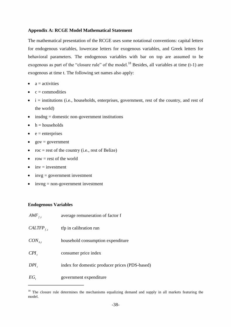
Appendix A: RCGE Model Mathematical Statement
The mathematical presentation of the RCGE uses some notational conventions: capital letters
for endogenous variables, lowercase letters for exogenous variables, and Greek letters for
behavioral parameters. The endogenous variables with bar on top are assumed to be
exogenous as part of the “closure rule” of the model.18
Besides, all variables at time (t-1) are
exogenous at time t. The following set names also apply:
a = activities
c = commodities
i = institutions (i.e., households, enterprises, government, rest of the country, and rest of
the world)
insdng = domestic non-government institutions
h = households
e = enterprises
gov = government
roc = rest of the country (i.e., rest of Belize)
row = rest of the world
inv = investment
invg = government investment
invng = non-government investment
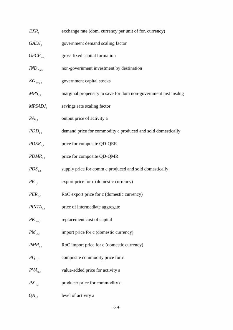
Endogenous Variables
tfAWF , average remuneration of factor f
tfCALTFP , tfp in calibration run
thCON , household consumption expenditure
tCPI consumer price index
tDPI index for domestic producer prices (PDS-based)
tEG government expenditure
18
The closure rule determines the mechanisms equalizing demand and supply in all markets featuring the
model.
Page 40
-39-
tEXR exchange rate (dom. currency per unit of for. currency)
tGADJ government demand scaling factor
tinvGFCF , gross fixed capital formation
tafIND ,, non-government investment by destination
tinvgKG , government capital stocks
tiMPS , marginal propensity to save for dom non-government inst insdng
tMPSADJ savings rate scaling factor
taPA , output price of activity a
tcPDD , demand price for commodity c produced and sold domestically
tcPDER , price for composite QD-QER
tcPDMR , price for composite QD-QMR
tcPDS , supply price for comm c produced and sold domestically
tcPE , export price for c (domestic currency)
tcPER , RoC export price for c (domestic currency)
taPINTA , price of intermediate aggregate
tinvPK , replacement cost of capital
tcPM , import price for c (domestic currency)
tcPMR , RoC import price for c (domestic currency)
tcPQ , composite commodity price for c
taPVA , value-added price for activity a
tcPX , producer price for commodity c
taQA , level of activity a
Page 41
-40-
tcQD , quantity sold domestically of domestic output c
tcQDER , QD-QER aggregate for comm c
tcQDMR , QD-QMR aggregate of comm c
tcQE , quantity of exports for commodity c
tcQER , quantity of exports to RoC for commodity c
tafQF ,, quantity demanded of factor f from activity a
tfQFS , supply of factor f
tcQG , quantity of government demand for commodity c
thcQH ,, quantity consumed of commodity c by household h
tacQINT ,, quantity of commodity c as intermediate input to activity a
taQINTA , quantity of aggregate intermediate input
tcQINV , quantity of investment demand for commodity c
tcQM , quantity of imports of commodity c
tcQMR , quantity of imports from RoC of commodity c
tcQQ , quantity of goods supplied domestically (composite supply)
tcQTROC , RoC tourism demand quantity of comm c
tcQTROW , RoW tourism demand quantity of comm c
tcQT , quantity of trade and transport demand for commodity c
taQVA , quantity of aggregate value added
tcQX , quantity of domestic output of commodity c
tREXR real exchange rate
tcRGDPFC , real GDP at factor cost (at constant base-year prices)
Page 42
-41-
tinvRGFCF , real gross fixed capital formation
tRSG real government savings
tSG government savings
tiSH , savings domestic non-government institution i
tSROC RoC savings (foreign currency)
tSROW foreign savings (foreign currency)
taTFP , total factor productivity index
tiiTR ,', transfers from dom inst insdng to inst ins
tfUERAT , unemployment rate for factor f
tWALRAS dummy variable (zero at equilibrium)
tfWF , average price of factor f
tafWFDIST ,, wage distortion factor for factor f in activity a
tfYF , factor income
tYG government revenue
tiYH , income of (domestic non-government) institution insdng
tfiYIF ,, income of institution ins from factor f
Parameters and Exogenous Variables
F
fish , share for inst ins in the income of factor f
timps
, marginal propensity to save for dom non-gov inst insdng
tcqg
, quantity of government demand for commodity c
tinvrgfcf
, real gross fixed capital formation
tata , rate of tax on producer gross output value
Page 43
-42-
tctq , rate of sales tax
tity , rate of direct tax on dom inst ins
tftf , rate of direct tax on factor income
taftfact ,, rate of factor use tax
tcte , export tax rate for commodity c
tctm , import tariff rate for commodity c
tiactrnsfr ,, transfers from insp to ins or factor
TR
fiish ,', share of inst ins in post-tax post-sav income of inst insp
tcpwe , export price for c (foreign currency)
tcpwm , import price for c (foreign currency)
tcpwer , export price for c to RoC (foreign currency)
tcpwmr , import price for c from RoC (foreign currency)
tcqdstk , changes in inventories
',ccicd trade and transport input of c per unit of comm cp produced and sold
domest
',ccice trade and transport input of c per unit of comm cp exported
',ccicm trade and transport input of c per unit of comm cp imported
',ccicer trade and transport input of c per unit of comm cp exported to RoC
',ccicmr trade and transport input of c per unit of comm cp imported from RoC
tcqtroc
, RoC tourism demand quantity of comm c
tcqtrow
, RoW tourism demand quantity of comm c
VA
af , share parameter for CES activity production fn
Page 44
-43-
VA
a efficiency parameter in the value added production fn for a
VA
a elasticity of substitution between factors
VA
a exponent in the value added production fn for a
tatfpexog , exogenous component of sectoral TFP
ca, yield of output c per unit of activity a
acica , intermediate input c per unit of aggregate intermediate
aiva aggregate value added coefficient for act a
ainta aggregate intermediate input coefficient for act a
LES
hc, marg shr of hhd cons on commodity c
cqhmin subsist cons of com c for hhd h
M
c Armington function share parameter for imports commodity c
DMR
c Armington function share parameter for composite QDMR commodity c
Q
c Armington function shift parameter for commodity c
Q
c elasticity of substitution between dom goods and imports for c
Q
c Armington function exponent for commodity c
E
c CET function share parameter for exports commodity c
DER
c CET function share parameter for composite QDER commodity c
X
c CET function shift parameter for commodity c
X
c elasticity of transformation between dom sales and exports for c
X
c CET function exponent for commodity c
MR
c Armington function share parameter for RoC imports commodity c
DD
c Armington function share parameter for domestic commodity c
Page 45
-44-
DMR
c Armington function shift parameter for commodity c
DMR
c elasticity of substitution between dom goods and imports for c
DMR
c Armington function exponent for commodity c
ER
c CET function share parameter for RoC exports commodity c
DS
c CET function share parameter for domestic commodity c
DER
c CET function shift parameter for commodity c
DER
c elasticity of transformation between dom sales and exports for c
DER
c CET function exponent for commodity c
roct constant price elasticity of RoC tourism demand (< 0)
rowt constant price elasticity of RoW tourism demand (< 0)
ccwts consumer price index weights
cdwts domestic sales price weights
fphillips elasticidad-desempleo del salario factor f
taffprd ,, productivity term for factor f in act a
velocidad movilidad del capital entre actividades
invccapcomp , quantity of commodity c per unit of investment inv
ng depreciation rate for non-government capital
g depreciation rate for government capital
Equations
The model equations are organized in the following eight groups: production, incomes and
savings, prices, international trade, final consumption, equilibrium conditions, miscellaneous,
and investment by destination (i.e., dynamics).
Production Function
Page 46
-45-
In the first place, we describe the production function, which is organized in two levels (see
Figure A.1). As shown in the figure, we use nested Leontief (i.e., fixed coefficients) and CES
(Constant Elasticity of Substitution) production functions. Equations (PF1) and (PF2) show
that value added ( aQVA ) and the aggregate of intermediate inputs ( aQINTA ) are a fixed
proportion of the activity production level ( aQA ), respectively.
aaa QAivaQVA (PF1)
aaa QAintaQINTA (PF2)
Equations (PF3) and (PF4) represent the first order conditions of the optimization problem
solved by the representative firm in each industry or activity (i.e., cost minimization/profit
maximization). The value added production technology is a CES function. The remuneration
to factor f paid by the activity a is computed as affWFDISTWF , , where afWFDIST , is a
“distortion” factor that allows modeling cases in which the factor remuneration differs across
activities.19
As we will see, this method to compute the remuneration of factor f in each
activity allows to easily selecting among alternative closures (i.e., mechanisms to equalize
supply and demand) in the factor markets.20
Equation (PF5) computes sectoral total factor productivity (TFP) as a function of (a) an
exogenous component, and (b) the size of the public infrastructure capital stocks. Thus, an
increase in the provision of public infrastructure of type invginf (e.g., roads) would have
positive impacts on sectoral TFP, more or less strong depending on the value assigned to the
invgatfpelas , elasticity parameter. In equation (PF5), variable 00
invgKG refers to the public capital
stock in sector invg in the base year. In other words, our model assumes that, based on
available empirical evidence, that public infrastructure has positive externalities on sectoral
TFP. For model calibration, the initial public capital stock can be estimated through
alternative methods; for example, based on recent data for public investments.
VAaVA
a
f
afaf
VA
af
VA
aaa FDfprdTFPQA
1
,,,
(PF3)
19
In this presentation we assume that its value is exogenous for labor and exogenous for capital; its value can be
computed by combining the social accounting matrix with employment data by activity.
20 Besides, for the factors considered as specific, equation (PF4) is interpreted as an equilibrium condition
between factor supply and demand.
Page 47
-46-
1
,
1
,
,,
,1
VAa
VAa
VAa
VAa
afa
VA
aa
VA
af
afaff
aaf fprdQVATFP
tfactWFDISTWF
PVAFD
(PF4)
invginfinvg
tfpelas
invg
tinvg
ttata
invga
KG
KGCALTFPtfpexogTFP
,
00
,
,, (PF5)
Individual intermediate inputs are also a fixed share of output. However, note that in equation
(PF6) intermediate inputs are a fixed share of the aggregate intermediate input which, in turn,
is a fixed proportion of output (equation (PF2)).21
aacac QINTAicaQINT ,, (PF6)
Equation (PF7) computes the production of each product on the basis of the ca, parameter,
which represents the production of product c per unit produced of activity a. Thus, following
the supply and use tables, our model differentiates between activities and
commodities/products. In addition, an activity can produce more than commodity and the
same commodity may be produced by more than one activity.
a
acac QAQX , (PF7)
21 Note that, unlike the acica , parameters, the Leontief technical coefficients are expressed as share of output.
Page 48
-47-
Figure A.1: production function
where ACT=activities, VA=value added, INTA=aggregate of intermediate inputs,
LAB=labor, CAP=capital, INT=intermediate consumption, DOM=domestic, and
IMP=imported.
Source: Author’s own elaboration.
Prices
Equation (PR1) implicitly defines the price of value added, as all other variables in that
equation are determined elsewhere in the model. For each activity, the price of its
intermediate input composite ( aQINTA ) is a weighted average of the prices of each of the
commodities that is demanded as an intermediate input (equation (PR2)), with acica , as
weights. As we have seen, acica , is the quantity of commodity c used as an intermediate input
in activity a per unit of aQINTA . The price of each activity is a weighted average of the
prices of the commodities it produces (equation (PR3)).
aaaaaaa QINTAPINTAQAtaPAQVAPVA 1 (PR1)
c
acca icaPQPINTA , (PR2)
c
ccaa PXPA , (PR3)
Trade with Rest of the Country
RoC Prices
ct
cctctcc icmrPQpwmrPMR , (TC1)
CES
DOM1
...IMPc
LAB...
CAP INT1
...INTc
ACT
LF
VA INT
CES LF
Page 49
-48-
ct
cctctcc icerPQpwerPER , (TC2)
QDD + QMR
DMRc
DMRc
DMRc
c
DD
cc
MR
c
DMR
cc QDQMRQDMR 1
(TC3)
DMRc
DD
c
MR
c
c
c
c
c
PMR
PDD
QD
QMR
1
1
(TC4)
cccccc QMRPMRQDPDDQDMRPDMR (TC5)
QDS + QER
DERc
DERc
DERc
c
DS
cc
ER
c
DER
cc QDQERQDER 1
(TC6)
1
1
DERc
ER
c
DS
c
c
c
c
c
PDS
PER
QD
QER
(TC7)
cccccc QERPERQDPDSQDERPDER (TC8)
Trade with Rest of the World
Equations (TW1) and (TW2) define domestic prices of exports ( cPE ) and imports ( cPM ),
respectively. It is assumed that the modeled economy is small; thus, world prices for exports
and imports are given ( cpwe and cpwm ; also, see below). The government can collect tariffs
on imports and taxes on exports, at rates ctm and cte , respectively. Besides, the model also
considers trade and transport margins applied to exports and imports; i.e., ccice ,' and ccicm ,'
represent the quantity of trade/transport commodity ct per unit of exports and imports of
commodity c, respectively.
ct
cctctccc icmPQpwmEXRtmPM ,.1 (TW1)
ct
cctctccc icePQpweEXRtePE ,.1 (TW2)
Equation (TW3) computes the demand price of the domestic product, by adding to its supply
price the corresponding trade and transport margin. Thus, parameter ccicd ,' refers to the
Page 50
-49-
quantity of commodity c’ (i.e., trade and transport; distribution services) that is required to
move one unit of domestic product c from the producer to the consumer.
ct
cctctcc icdPQPDSPDD , (TW3)
Qc
Qc
Qc
c
DMR
cc
M
c
Q
cc QDMRQMQQ 1
(TW4)
Qc
DMR
c
M
c
c
c
c
c
PM
PDMR
QDMR
QM
1
1
(TW5)
ccccccc tqQMPMQDMRPDMRQQPQ 1 (TW6)
Demand of Products -- Dom + Exp
Xc
Xc
Xc
c
DER
cc
E
c
X
cc QDERQEQX 1
(TW7)
1
1
Xc
E
c
DER
c
c
c
c
c
PDER
PE
QDER
QE
(TW8)
cccccc QEPEQDERPDERQXPX (TW9)
Incomes and Savings
Factors. Equation (YF1) computes the total income of factor f. The first term on the right
hand side corresponds to total factor payments from activities. Besides, factor f can receive
transfers from the rest of the world. In turn, equation (YF2) computes the income received by
each institution for being the owner of factor f, net of the applicable (direct) tax on factor
income.
rocfrowf
a
afafff trnsfrEXRtrnsfrFDWFDISTWFYF ,,,, (Y1)
ff
F
fifi tfYFshYIF 1,, (Y2)
Domestic Non-Government Institutions; insdngi . Households. The income of the domestic
non-government institution i(insdng) (i.e., households and enterprises) is the sum of two
elements: (1) factor income, and (2) transfers from other institutions (see equation (Y1)).
Equation (Y2) computes the marginal propensity to save for the domestic non-government
Page 51
-50-
institutions. Initially, variable MPSADJ is equal to one.22
Equation (Y3) computes the value
of savings for each domestic non-government institution in the model, as a linear function of
disposable income.
rocirowi
insdngi
iigovi
f
fii trnsfrEXRtrnsfrTRCPItrnsfrYIFYH ,,
'
',,,
(Y3)
MPSADJmpsMPSii (Y4)
iiii tyYHmpsSH 1 (Y5)
iii
TR
iiii YHtyMPSshTR 11,',' (Y6)
Households. Equation (H1) computes the consumption spending by households as their
income net of transfers to other institutions, savings, and direct taxes.
hhh
i
TR
hih YHtyMPSshCON
111 , (H1)
Local Government. Equation (G1) computes government income as the sum of three
elements: (1) tax collection, (2) transfers from other institutions, and (3) factor income. Note
that transfers from the rest of the world are multiplied by the exchange rate so that they are
expressed in local currency. The government uses its income to provide goods and services
and make transfers to other institutions (equation (G2)). Equation (G3) computes government
savings as the difference between current income (YG ) and current spending ( EG ).
f
fgov
insdng
insdnggovrocgovrowgov
af
afafaff
f
ff
ccccc
a
aaa
c
ccc
c
ccc
h
hh
YIF
TRtrnsfrEXRtrnsfr
tfactFDWFDISTWFYFtf
QMPMQDMRPDMRtq
QAPAta
QEpweEXRte
QMpwmEXRtm
YHtyYG
,
,,,
,
,,,
.
.
(G1)
22 Besides, in this presentation it is assumed that MPSADJ is an exogenous variable.
Page 52
-51-
govrocgovrow
insdngi
govi
c
cc trnsfrEXRtrnsfrCPItrnsfrQGPQEG ,,,
(G2)
EGYGSG (G3)
Central Government. Equations (G4)-(G6) are similar to equations (G1)-(G3) but refer to the
central government. As we see, both levels of government tax the same tax base.
Consequently, the model captures the interaction between the tax policies of the various
levels of government.
f
fgovc
govgovc
insdng
insdnggovcrocgovc
af
afafaff
f
ff
ccccc
a
aaa
c
ccc
c
ccc
h
hh
YIF
trnsfrTRIItrnsfr
tcfactQFWFDISTWFYFtcf
QMPMQDMRPDMRtcq
QAPAtca
QEpweEXRtce
QMpwmEXRtcm
YItcyYGC
,
,,,
,
,,,
.
.
(G4)
govcgov
insdngi
govi
c
cc trnsfrCPItrnsfrQGCPQEGC ,,
(G5)
EGCYGCGCSAV (G6)
Rest of the World. The rest of the world is represented through the current account of the
balance of payments, expressed in foreign currency (equation (RW1)). The left (right) hand
side shows the inflows (outflows) of foreign exchange. The current account balance of the
balance of payments is the negative of foreign savings (equation (RW2)).
EXR
YIF
EXR
TR
trnsfrQMpwm
SROWEXR
QTROWPQ
trnsfrQEpwe
f
frow
insdngi
irow
govrow
c
cc
c
cc
ac
rowac
c
cc
,,
,
,
(RW1)
Rest of the Country
Page 53
-52-
f
froc
insdngi
irocgovroc
c
cc
c
cc
ac
rocac
c
cc
YIFTRtrnsfrQMRpwmr
SROCQTROCPQtrnsfrQERpwee
,,,
,
(Y13)
Final Consumption
Household consumption expenditure is distributed across commodities according to a Stone-
Geary utility function, from which a linear expenditure system is derived (equation (FD1)).
Equation (FD2) computes the investment demand of commodity c. It is assumed that the
commodity composition of investment is exogenous – see parameter invccc , . Thus, if there is
an increase in investment, investment demand for all goods and services will increase in the
same proportion.23
It is assumed that the commodity composition of government
consumption is also fixed at its initial values. Initially, variable GADJ is equal to one.
Equation (FD4) is the total demand for commodities that provide trade and transport margins;
the demand for such commodities is linked to domestic products, imports and exports.
'
,''
,
,,
c
hcch
c
LES
hc
hchc qhminPQCONPQ
qhminQH
(FD1)
inv
invinvcc RGFCFccQINV , (FD2)
GADJqgQGcc (FD3)
'
'','','','','',
c
cccccccccccccccc QERicerQMRicmrQDicdQEiceQMicmQT (FD4)
Tourism Demand (RoC and RoW); exogenous if eta_roct = 0 and eta_rowt = 0. Note that
although tourists from the rest of the Belize do not need to change currencies, a real exchange
rate exists between the modeled region of Belize and the rest of the Belize.
roct
c
ccc
PQ
PQqtrocQTROC
0 (FD5)
rowt
EXRPQ
EXRPQqtrowQTROW
c
ccc
00 (FD6)
Unemployment
23
This presentation assumes that investment is considered as an endogenous variable; see below the discussion
of macroeconomic closure rule.
Page 54
-53-
Equation (U1) is the wage curve for factor f (see Blanchflower and Oswald (1994)). It is
assumed that there is a negative relation between the real wage and the unemployment rate,
as the value of the phillips parameter is negative. In fact, Blanchflower and Oswald (2005)
report a value for the unemployment-elasticity of wage close to -0.1 for a large number of
countries. Note that the wage curve is consistent with several stories to explain the presence
of unemployment for the labor market, such as efficiency wages, unions with bargaining
power, among others.
fphillips
f
fff
UERAT
UERAT
CPI
WF
CPI
WF
00
0
(U1)
Equilibrium Conditions
Equation (EQ1) is the equilibrium condition in the market for factor f. As will be shown, this
model presentation assumes that all factor supplies are exogenous. However, the supply of
each factor ( fFS ) can be exogenous or endogenous depending on the selected closure rule.
Equation (EQ2) is the equilibrium condition between supply and demand for each
commodity. Total supply, composed of domestic and imported varieties, is used for
household consumption, intermediate consumption, investment, local and central government
consumption and changes in inventories. Equation (EQ3) is the savings-investment balance;
three are the institutions that contribute to total savings: domestic non-government
institutions (i.e., households and enterprises), government, and the rest of the world. The
variable WALRAS must be zero in equilibrium.
a
afff FDUERATFS ,1 (EQ1)
ccc
ccccc
a
ac
h
hc
QQQTROWQTROC
qdstkQTQGCQGQINVQINTQH
,,
(EQ2)
insdngi
i
c inv
invcc SROCSROWEXRSGSHGFCFqdstkPQ . (EQ3)
Miscellaneous
Equation (MIS1) defines the consumer price index as a weighted average of the composite
commodity prices; the weights are the shares of each commodity in private (i.e., household)
consumption. In this presentation CPI is the model numeraire (see below). Equation (MIS2)
defines the producer domestic price index as a weighted average of the prices of domestic
Page 55
-54-
output sold in the domestic market. Equation (MIS3) defines the real exchange rate, as the
ratio between the nominal exchange rate and the producer domestic price index. Finally,
equation (MIS4) computes the real GDP at factor cost.
CPIcwtsPQc
cc
DPIdwtsPDSc
cc
DPI
EXRREXR
a
aa QVAPVARGDP 00
Investment by Destination; Dynamics
Lastly, this group of equations presents the model dynamics. Specifically, the mechanisms
used to assign each period private and public investment among sectors are presented. As will
be shown, a distinction is made between private and public capital stocks; this is particularly
relevant given our interest in simulating increases in the government investment of public
infrastructure.
Non-Government Sector. In this case, investment in each period increases the capital stock
available in the next period. Then, we need to determine how the new capital is distributed
among industries. In our model, for private investment (i.e., households and/or enterprises)
we assume that the new capital is distributed across activities based on sectoral differences in
the rates of return on capital. Thus, sectors with a relatively higher (lower) capital rate of
return receive a relatively larger (smaller) share of the new capital.
Equation (DP1) computes the price of one unit of capital type “inv”; the new capital is
assembled using a fixed coefficient production function. Equation (DP2) computes the real
gross fixed capital formation, which refers to the quantity of new units of the capital good
that will be available to produce the next period. Equation (DP3) computes the average rate
of return for private capital, as the ratio between total capital income and total capital stock.
Equation (DP4) computes the share of each activity in the new capital stock, following the
explanation on the previous paragraph. The parameter, which varies between zero and
one, measures the degree of capital mobility among productive sectors. When is zero,
investment is distributed among sectors only based on the initial share of each sector in the
total capital stock. When is positive, investment is distributed among sectors also based on
Page 56
-55-
the relative capital returns. Finally, equation (DP5) shows how sectoral capital stocks are
updated.
c
cinvcinv PQcapcompPK , (DP1)
inv
invinv
PK
GFCFRGFCF (DP2)
a
af
a
affaf
fFD
WFDISTWFFD
AWF,
,,
(DP3)
11
,
'
',
,
,
k
akk
a
ak
ak
invngakAWF
WFDISTWF
FD
FDRGFCFIND (DP4)
1,,1,, 1 akk
ng
kak INDFDFD (DP5)
Government Sector. For the government, investment can be determined in two alternative
ways: (1) as a policy variable (i.e., exogenously) (equation (DG6)), or (2) as a residual to
balance the government budget. Equation (DG6) updates the public capital stocks of period t
using public investment from period t-1. For example, an increase in public investment in
infrastructure would be modeled as an increase in the value of the relevant element of the
invgrgfcf parameter. Then, an increase in invgKG would be obtained that, in turn, would
positively impact on the sectoral TFP (see equation (PF7) above). As mentioned, the model
allows for the identification of more than one type of public capital; for example, different
infrastructure sectors such as roads, communications, energy, among others.
invginv rgfcfRGFCF (DG6)
1,1,, 1 invginvg
g
ainvg RGFCFKGKG (DG7)
Page 57
-56-
Appendix B: Technical Note on the Construction of the RSAM for Belize Cayo District
B.1. Introduction
The aim of this technical appendix is to document in detail the steps that have been followed
to build the Regional Social Accounting Matrices (RSAM) for the Belize Cayo District that
was used to calibrate our Regional Computable General Equilibrium (RCGE) model24
, an
extended version of the (recursive) dynamic computable general equilibrium model
developed for the IDB for tourism development strategy analysis. For a comprehensive
description of the RCGE, see Appendix A.
In outline, we proceed as follows. The basic concepts that define the RSAM are introduced in
Section B.2. The data requirements to construct the RSAM for the Belize Cayo District are
identified and described in Section B.3. The next section spells out the steps that have been
followed to construct the RSAM, starting from a national SAM.
B.2. A Regional Social Accounting Matrix
A SAM (and a RSAM) is a matrix representation of the interrelationships existent on an
economy at the level of individual production sectors, factors, and institutions. As stated in
Round (2003), “it is a comprehensive, flexible, and disaggregated framework which
elaborates and articulates the generation of income by activities of production and the
distribution and redistribution of income between social and institutional groups”.
The SAM is composed of accounts. For each of these, a cell represents a payment column-
wise and a receipt row-wise. Hence, columns represent expenditures for each account
whereas rows record the matching incomes. Due to the accounting consistency of the SAM,
total expenditure of every account must be equal to its total income. In other words, the total
of every row must be equal to the corresponding total of the column. The basic structure of a
RSAM is presented in Table B.1.
24
Of course, the procedure described here can be used to build a RSAM for other regions of Belize.
Page 58
-57-
Table B.1: stylized regional social accounting matrix
where com = commodities, dom-prod = domestic production, gov = government, RoC = rest
of the country, RoW = rest of the world, IO = intermediate consumption, VA = value added,
T = taxes, M = imports, INC-F = factor income to/from abroad, TR = transfers, C = private
consumption, G = government consumption, E = exports, I = investment, SH = households
savings, SG = government savings, and SF = foreign savings.
Source: Authors’ own elaboration.
The logic behind the SAM transactions is the following. Activities buy intermediate inputs;
pay for factors of production, thus generating the value added at factor prices; and pay
indirect taxes. All these expenditures are financed with the payments that each activity
receives for the sale of its output.
Aggregate supply and demand are both recorded in the commodities accounts. For each
commodity, the corresponding account records for the sales of the aggregate supply
(domestic output plus imports from the rest of the country and the rest of the world, and
related taxes) as follows: to activities as these demand intermediate goods; to households,
government and investment as these demand final goods; and to the rest of the country and
the rest of the world as this demands the region’s exports.
income activities com factors households gov local gov central RoC RoW sav-inv total
activities dom-prod inc firms
com IO C G G E E I demand
factors VA INC-F INC-F inc fac
households VA TR TR TR TR inc hhd
gov local T T T TR TR inc gov loc
gov central T T inc gov cent
RoC M INC-F TR TR out LCU
RoW M INC-F TR TR out forex
sav-inv SH SG local SG central SROC SROW sav
total spnd firms supply spnd fac spnd hhd spnd gov loc spnd gov cent in LCU in forex inv
spending
Page 59
-58-
Factors earn returns from their involvement in domestic and foreign (including the RoC)
production, and they distribute them, net of taxes, to their owners (generally, households and
enterprises).
Institutions (households, enterprises25
, government, rest of the country, and rest of the world)
receive incomes from production factors and (net) transfers that can be either spent in
purchasing commodities or saved.
Savings from household, the local and central governments (that is, the current account
balance), the rest of the country, and the rest of the world (that is, the current account balance
with opposite sign) add to aggregate savings and these, in turn, are equal to the level of
investment of the regional economy.
Regional gross domestic product (RGDP) at factor cost builds as activities remunerate factors
of production (that is, value added). RGDP at market prices equals RGDP at factor cost plus
indirect taxes and tariffs, which should also be equal to total final demand plus exports minus
imports, both from RoC and RoW.
B.3. Data
The main sources of information when constructing a national/regional SAM tend to be
national supply and use tables, and other databases such as regional accounts, fiscal data, and
the balance of payments. The supply and use table provides information on production,
intermediate consumption, final demand (i.e., household and government consumption),
exports, and value added. In our case, we first built a national SAM that was later on
regionalized using non-survey techniques. In doing so, the national supply and use table was
combined with regional data on sectoral employment from the most recent household income
and expenditure survey, the Belize Household Expenditure Survey 2008-2009.
In our case, the SAM and RSAM base year was selected based on the available information.
Specifically, the more recent year with a complete set of national accounts data was selected
as the base year, 2013. As will be discussed, in the case of Belize, the national accounts do
not provide a supply and use table.
B.4. Steps in Building the RSAM
25
The SAM and RSAM built do not separate enterprises from the households. A single account, named hhd, is
taken as representative of the domestic private sector.
Page 60
-59-
Typically, we start with a relatively aggregate SAM that, in a stepwise fashion is
disaggregated, drawing on additional data in different areas.26
Specifically, the process
followed has a top-down structure, entailing three steps: (i) construction of an aggregate
national SAM (hereafter, Macro SAM), (ii) disaggregation of the Macro SAM into a matrix
with a relatively large sectoral breakdown (hereafter, SAM), and (iii) regionalization of the
SAM to make it suitable for the calibration of our regional CGE model (hereafter RSAM).
B.4.1. Macro SAM
In the first step of the RSAM building, a very schematic representation of the national
economy was generated, using macroeconomic aggregates from the national accounts. In
case needed, information from other sources, adjusted to keep the consistency, was next used
to improve the representation of the economy. In particular, data on public finances and
balance of payment were factored in to complete the construction of the national Macro
SAM; especially to adjust the current account balances of the government and the rest of the
world, among others. Specifically, the data sources are:
national accounts data at current prices from the Statistical Institute of Belize (SIB),
including gross domestic product by activity and expenditure on gross domestic product;
data on tax collection and government revenues and expenditures from Belize Ministry of
Finance, Belize Department of General Sales Tax, the IDB (2016), and IMF 2015 Article
IV Consultation;
balance of payments from the Central Bank of Belize; and
supply and use table for Ecuador 2007 and 2013 (see below).
The estimated Macro SAM is presented in Table B.2, where the following abbreviations are
used:
act = activities
com = commodities
f-lab = labor
f-cap = capital
tax-act = activity taxes
tax-com = commodity taxes
sub-com = commodity subsidies
26
The top-down approach for the SAM-building process is described with more detail in Reinert and Roland-
Holst (1997).
Page 61
-60-
tax-imp = import tariffs
tax-dir = direct taxes
hhd = households
gov = government
row = rest of the world
sav = savings
invng = non-government investment
invg = government investment
dstk = stock change
Table B.2: Macro SAM for Belize 2013 (BZ$ million)
Source: Authors’ own elaboration.
In building the Macro SAM, and due to the lack of Belizean data, the 2013 Ecuadorian
supply and use table was used to split total value added net of “other taxes on production”
between payments to labor and capital.27
In Table B.2, capital payments comprise gross
operating surplus and mixed income.
B.4.2. National SAM
At this stage, the aim became to build more disaggregated SAM, which would be as large as
the data available would allow it. Specifically, the main inputs to initiate the disaggregation
for activities and commodities of the Macro SAM were
27
In the main text we discuss the reason for using the Ecuadorian supply and use table to build the Belize SAM.
act com
f-lab
f-cap
tax-
act
tax-
imp
tax-
com
tax-
dir
hhdgo
vro
wsa
vin
vng
invg
dstk
tota
l
act 2,806 2,806
com 2,325 492 1,977 388 192 33 5,406
f-lab 1,504 5 1,509
f-cap 1,295 7 1,303
tax-act 7 7
tax-imp 160 160
tax-com 286 286
tax-dir 249 249
hhd 1,496 974 194 208 2,872
gov 93 7 160 286 249 1 796
row 2,154 13 236 53 9 2,465
sav 244 101 268 613
invng 388 388
invg 192 192
dstk 33 33
total 2,806 5,406 1,509 1,303 7 160 286 249 2,872 796 2,465 613 388 192 33
Page 62
-61-
sectoral output (i.e., value added at basic prices) information from national accounts
provided by the SIB;
sectoral exports and imports of goods provided by the SIB and COMTRADE (United
Nations Commodity Trade Statistics Database);
sectoral exports and imports of services from the balance of payments;
sectoral tariff rates from TRAINS (UNCTAD - Trade Analysis Information System); and
Ecuador 2013 supply and use table.
In Table B.3, we list the 18 activities and commodities identified in the Belize
(national/regional) SAM. Certainly, the number of sectors could be increased once additional
sectoral output data becomes available.
Table B.3: activities and commodities in the Belize (national) SAM 2013
Source: Authors’ own elaboration.
In addition, various other complementary adjustments were implemented during the building
process of the SAM:
non-profit final consumption was added to be part of the private sector account, hhd;
financial intermediation services indirectly measured were distributed across sectors
based on their estimated intermediate consumption of financial services;
Crops
Livestock
Forestry
Fishing
Mining
Food and beverages
Textiles
Other manufacturing
Electricity and water
Construction
Trade
Hotel and restaurants
Transport
Post and telecommunications
Financial intermediation
Real estate, renting and bus svc
Community, social and pers svc
General government services
Page 63
-62-
direct purchases were consolidated with the relevant sectors28
;
imports, exports and cif/fob adjustments are all accounted for in the single SAM account
pertaining to the rest of the world, “row”;
split of gross operating surplus/mixed income into its two components using the 2007
Ecuador supply and use table; mixed income was associated with non-salaried workers;
GTAP (Global Trade Analysis Project) data was used to split the sectoral gross operating
surplus among payments to capital, land, and natural resources used in forestry, fishing,
and mining (coal, petroleum and gas, metals, and other);
trade and transport margins were split between domestic products, imports, and exports;
we assumed that the distribution margins requirements are proportional to the
corresponding transactions; and
the stock variation is a component of the total gross investment; this is expressed in the
SAM as a payment done by the savings-investment account, savings (“sav") to the stock
variation account, “dstk”; and
in the current version of the SAM, the stock variation account was used to balance the
commodity accounts of the SAM.
Disaggregation of Gross Fixed Capital Formation
Typically, a SAM specifies the investment in a slightly different setup to that of the RSAM
for our model. The RSAM for our RCGE includes, at least, two investment accounts: one for
the private sector, and one for the services that are provided by the government. This
disaggregation implies that investment by sector of origin and by sector of destination had to
be specified. As a first step, we assumed that the composition of the capital good is the same
independently of the sector of destination by keeping the disaggregation of investment by
sector of origin as this is initially accounted for in the national SAM. Next, based on regional
evidence, we assumed that public investment demand is biased towards construction services.
On the other hand, private investment demand is biased towards machinery and equipment
(see Table B.4).
28
Direct purchases usually represent the expenditure on transport and communication services of the
governmental and private sector abroad and from foreign individuals in the country.
Page 64
-63-
Table B.4: investment demand sectoral composition
Source: Authors’ own elaboration based on national accounts data for Costa Rica, Ecuador,
Guatemala, and Mexico.
Disaggregation of Labor Payments
In the SAM used to calibrate our RCGE model, each labor category (i.e., salaried and non-
salaried) was disaggregated into two types according to the educational level as follows: (i)
unskilled, for workers with less than nine years of education (i.e., less than lower secondary);
and (ii) skilled, for individuals who have nine or more years of education (i.e., completed
lower secondary, with or without [incomplete/complete] tertiary education). In order to
conduct such disaggregation, we used information on labor payments by sector, labor
category (salaried/non-salaried) and skill level from the Household Expenditure Survey for
the year 2008-2009, conducted by the SIB (see Table B.5). The HES 2008-2009 is the latest
available household income and expenditure survey in Belize; it covers 11,442 individuals in
3,023 households in all of Belize. The HES 2008-2009 was processed following the
SEDLAC (Socio-Economic Database for Latin America and the Caribbean) guidelines
(World Bank and CEDLAS, 2012). Not surprisingly, the HES 2008-2009 does not provide
enough information for all labor categories and activities in the SAM. Thus, two or more
sectors in the national accounts were linked to the same activity in Table B.5.
Commodity Private Public Total
Machinery and equipment 38.4 11.0 31.8
Construction services 61.6 89.0 68.2
Total 100 100 100
Page 65
-64-
Table B.5: share of each labor skill level in total labor payments by sector and labor category
(salaried/non-salaried), (percent)
Source: Authors’ own elaboration based on HES 2008-2009.
B.4.3. Regional SAM for the Cayo District
The standard national SAM was regionalized to reflect the productive structure of the Belize
Cayo District, in order to make it suitable to calibrate our RCGE model. The regional SAM
for a single-region will have exactly the same aspect as the national SAM, but imports will
also include inflows coming from other regions within Belize and final demand will also
comprise of exports to other regions within Belize. Ideally, the RSAM would have dedicated
accounts for the local and the central government levels (see below).
In estimating our non-survey RSAM, the technical coefficients matrix was assumed to be
equal to its national counterpart, which is called the “national technology assumption”. It is
convenient to mention what these technical coefficients mean: they express the amount of
input of commodity c per unit of output of activity a, regardless of the geographic origin of
input of commodity c. This means that the national inter-industry transactions matrix to be
used as a starting point has to be a total flow matrix, thus including both nationally produced
and imported inputs (i.e., the cell IO in Table B.1). So, the implicit hypothesis is that
technology, in the production function sense, is spatially invariant within Belize (Lahr, 1993).
In our case, the regionalization of production was carried using the regional proportion of
industrial’s employment (see Table B.6). Thus, our key assumption is that labor productivity
(i.e., output per worker) is the same at the regional and at the national levels. Specifically, the
Sector
Salaried,
unskilled
Salaried,
skilled
Salaried,
total
Non-salaried,
unskilled
Non-salaried,
skilled
Non-salaried,
total
Crops + Livestock 88.7 11.3 100.0 92.0 8.0 100.0
Forestry 50.4 49.6 100.0 100.0 0.0 100.0
Fishing 85.7 14.3 100.0 96.8 3.2 100.0
Mining 64.3 35.7 100.0 97.9 2.1 100.0
Food and beverages 40.4 59.6 100.0 42.9 57.1 100.0
Textiles 58.1 41.9 100.0 81.4 18.6 100.0
Other manufacturing 45.0 55.0 100.0 66.2 33.8 100.0
Electricity and water 20.0 80.0 100.0 3.6 96.4 100.0
Construction 72.3 27.7 100.0 83.1 16.9 100.0
Trade 31.8 68.2 100.0 62.0 38.0 100.0
Hotel and restaurants 41.9 58.1 100.0 69.5 30.5 100.0
Transport 62.9 37.1 100.0 18.4 81.6 100.0
Post and telecommunications 9.6 90.4 100.0 0.0 100.0 100.0
Financial intermediation 11.2 88.8 100.0 . . .
Real estate, renting and bus svc 15.9 84.1 100.0 3.7 96.3 100.0
Community, social and pers svc 24.6 75.4 100.0 34.6 65.4 100.0
General government services 19.8 80.2 100.0 . . .
Total 41.4 58.6 100.0 57.6 42.4 100.0
Page 66
-65-
Household Expenditure Survey 2008-2009 identifies the following 17 activities or industries:
Crops and Livestock; Forestry; Fishing; Mining; Food and beverages; Textiles; Other
manufacturing; Electricity and water; Construction; Trade; Hotel and restaurants; Transport;
Post and telecommunications; Financial intermediation; Real estate, renting and business
services; Community, social and personal services; and General government services.
Table B.6: share of sectoral employment by district (percent)
Source: Authors’ own elaboration based on HES 2008-2009.
For final demand components, the following assumptions were made:
regional household consumption and private investment estimated based on the regional
income share (i.e., regional income in national income);
regional government current and capital spending based on population share (i.e., regional
population in national population);
the share of exports in total sectoral output at the regional level is assumed equal to the
share of exports in total sectoral output at the national level;
the share of imports in total sectoral consumption (intermediate and final) at the regional
level is assumed equal to the share of imports in total sectoral consumption at the national
level;
Sector Corozal
Orange-
Walk Belize Cayo
Stann-
Creek Toledo Total
Crops + Livestock 19.2 20.4 5.7 17.5 21.0 16.2 100.0
Forestry 10.6 16.7 16.3 53.3 3.2 0.0 100.0
Fishing 18.1 1.0 27.6 16.7 32.1 4.5 100.0
Mining 3.6 0.0 7.7 31.1 0.0 57.6 100.0
Food and beverages 5.3 24.3 34.8 21.4 12.9 1.3 100.0
Textiles 14.1 7.6 28.8 31.2 15.7 2.7 100.0
Other manufacturing 4.9 30.2 18.0 35.8 5.6 5.5 100.0
Electricity and water 4.0 8.8 49.6 25.7 6.6 5.3 100.0
Construction 12.8 16.8 31.8 26.1 9.0 3.5 100.0
Trade 19.6 18.8 31.5 21.6 3.8 4.6 100.0
Hotel and restaurants 12.3 3.1 51.6 16.8 10.7 5.5 100.0
Transport 10.2 10.2 48.4 16.5 11.7 3.1 100.0
Post and telecommunications 0.0 19.8 68.9 9.4 1.9 0.0 100.0
Financial intermediation 9.8 10.3 65.5 9.8 3.6 1.1 100.0
Real estate, renting and bus svc 4.0 3.0 62.4 22.4 4.4 3.8 100.0
Community, social and pers svc 10.3 11.5 39.4 22.9 8.4 7.5 100.0
General government services 8.4 5.6 42.9 33.5 4.6 5.0 100.0
Total 12.6 14.0 34.5 22.3 9.7 6.8 100.0
Page 67
-66-
the regional share of factor income to/from the rest of the world is equal to the national
share of factor income to/from the rest of the world;
the inter-regional imports and exports were estimated using commodity balance method
(see below);
regional household and government savings are estimated as residuals, once
corresponding current incomes and expenditures are known;
The commodity balance method used for estimating the inter-regional imports and exports
can be explained as follows (see Sargento, 2009). Let us define regional demand of
commodity c by rcd , . For any region, the following balance must hold:
rocrcrowrcrroccrrowcrcrc exexmmqd ,,,,,,,,,,
where
rcq , = regional output
rrowcm ,, and rroccm ,, = imports from rest of the world and rest of the country,
respectively
rowrce ,, and rocrce ,, = exports to rest of the world and rest of the country, respectively
This means that regional demand of commodity c is satisfied with regional output to which
are added regional imports and from which regional exports are subtracted. Based on this
balance, the commodity balance method is applied as follows:
If rcrc dq ,, , then it is assumed that the region has the capacity to provide all the
requirements of c in region r.
If rcrc dq ,, , it is assumed that the self-sufficiency of the region is limited to the
proportion rcrc dq ,, . Thus, the remaining regional demand will have to be fulfilled by
imports coming from outside the region; in our case, given that imports from RoW were
estimated, from the remaining regions.
Foreign Tourism Demand
Page 68
-67-
In order to single out foreign tourism demand, we combined information from (a) national
balance of payments, (b) tourist arrivals from SIB, (c) the sectoral information for the Hotels
and restaurants sector in the national accounts, and (d) the Tourist Exit Survey conducted in
Belize during February-March 2016. Specifically, from the last source of information we
extracted the commodity composition of foreign tourist demand that visit the Cayo District as
their primary destination. In Table B.7 we show the average per capita and per day spending
by commodity in the RSAM. In this version of the RSAM, due to the lack of data, we were
no able to also single out domestic tourism demand.29
Table B.7: average foreign tourists’ daily expenditure by commodity in the RSAM
(US$ and percent share)
Source: Authors’ own elaboration
In Section 3 of the main text, some statistics that were obtained from the national 2013 Belize
and 2013 Cayo District SAMs are presented.
29
However, the model can handle – as separate entities -- both foreign and domestic tourism demand.
Sector US$ share%
Food and beverages 8.1 4.1
Other manufacturing 5.3 2.6
Hotel and restaurants 80.4 40.1
Transport 54.6 27.3
Post and telecommunications 2.9 1.4
Other services (e.g., recreation) 49.0 24.5
Total 200.3 100.0
Page 69
-68-
Appendix C: Processing of HES 2008-2009
The database presents a wide format, so each line should identify one household (variable
HHID). Nevertheless, we found 14 cases with repeated HHID numbers, so we omitted these
(duplicated) ids. The wide format implies that we have to reshape the database to match the
individual questions of the different sections of the survey.
Merging of Section
As usual, the HES 2008 data is organized in several files that we had to merge. Specifically,
we found out that the only way to connect the different sections of the HES 2008 is by using
the person number inferred from the variable names. For example, consider the variable
Q16A11, where Q16 refers to the Section itself (Section 16 - Income), A refers to subsection
(in this example, the income section has four parts), then 1 refers to person number, and the
last 1 denotes the question number. Of course, we repeated this procedure in each of the
sections in order to merge the whole database.
Expenditure Sections
In the HES 2008, there are two different sources for expenditure variables. According to BIS,
the most complete and reliably source is the general survey, with 11 sections devoted to
capture the different expenses incurred by households. However, this source does not include
food expenses, consumed at home or at a restaurant. Therefore, we turn to the second source
of information available: the household record of daily expenditure. It includes (especially)
food and many other items. Specifically, this file contains a list that includes all expenditures
incurred by each household during the last two weeks. Then, after merging both databases,
we have a matching of 91.92% -- 281 household ids in the diaries survey are not present in
the general survey.
In all cases, we always select the variable “value” or “cost” reported in the questionnaire,
without taking into account the quantities purchased. Implicitly, we assume that households
tend to report the total expense in each category/product. In most cases, expenditure items are
reported on an annual basis. Thus, we annualized those that are not. In particular, we had to
annualize food and beverages (category 1) and restaurant and catering services (category 10).
As we mentioned, both categories were estimated from the household record of daily
expenditure. Thus, given that it captures expenditures incurred by each household during the
last two weeks, to annualize those categories we multiplied every single purchase by 24.
Based on a general classification, we define the following 12 expenditure categories.
Page 70
-69-
1. Food and beverages: this group is the only one based on information taken from the
household record of daily expenditure. It includes food and beverages consumed at the
household. COICOP product classification is used so we can classify food products and
calculate food expenses.
2. Clothing and footwear: purchases of ready-made clothes, tailoring and dressmaking costs,
repairs and alterations costs.
3. Housing, water, electricity, gas and other fuels: rents paid by renters, electricity bills,
water bills, cable TV bills, internet bills, garbage collection bills and cooking fuel purchases.
4. Furnishing, household equipment and routine household maintenance: repairs and
maintenance to the rental unit, costs for houses under construction, addition and
improvements for houses, fumigation costs, domestic helper costs, childcare costs,
cutting/yard cleaning costs, other regular household services, furniture, appliances and
textiles purchased for the household.
5. Health: premium payments (not covered by health insurance) for accidents,
hospitalization, maternity, surgery, x-ray, lab fees, anesthesia, ambulance, physician’s fees,
dental care, and purchases of medicines and medical supplies. In this case, we noticed that the
questionnaire does not include a question to know the amount paid for health insurance when
it is paid directly by the user.
6. Transport: operating expenses (gasoline, insurance, vehicle rental, etc.), servicing and
repairs (including parts and supplies costs) for private transport, public transportation (other
than vacation and business travel) including air, sea, bus and taxi transportation.
7. Communication: telephone bills, internet bills, phone cards purchases and internet coffee
usage.
8. Recreation and culture: expenditures on entrance fee for cinema concerts and sports
games, night clubs (entrance fee, drinks, etc.), casino, newspapers, books (other than school
books), magazines, hobbies, fairs/shows, weddings, funerals, baby showers, gifts/greeting
cards, parties (other than food), flowers, veterinary expenses (for pets), pet food, other pet
expenses, boledo/lottery/lotto tickets, postage, stationery (exclude school-related items),
courier service, church contributions and other charitable contributions. It also comprises
local travel expenses; including air fare, sea fare, bus fare, taxi, travel in personal vehicle,
gasoline, hotel, meals, tips, entertainment (tours, nightclubs, museums, sports events, etc.),
package tours and excursions and other travel expenses (rentals, souvenirs, etc.).
Page 71
-70-
9. Education: expenditures on tuition, exam fees, other educational fees,
books/supplies/equipment, special lessons, boarding/lodge, uniforms and others.
10. Restaurant and catering services: we had to estimate food expenses outside the
household. Specifically, the diaries database provides a “business type” variable, that
indicates the type of business or place from which the item was bought, e.g., supermarket.
Therefore, we selected bars, restaurants, fast food outlets, coffee shops and caterings to
estimate expense on those places.
11. Miscellaneous goods and services: expenses on haircuts, perms/relax, manicure, laundry
service, spa services, music lessons, fitness classes, life insurance and other expenditures, not
classified previously and declared in section 19.
12. Purchases in the rest of the world: foreign travel expenses; including air fare, sea fare,
bus fare, taxi, travel in personal vehicle, gasoline, hotel, meals, tips, entertainment (tours,
nightclubs, museums, sports events, etc.), package tours and excursions and other travel
expenses (rentals, souvenirs, etc.).
Finally, total household expenditure is the sum of all categories. In order to obtain household
per capita expenditure, we computed the ratio between this total amount and the number of
individuals that compose each (primary) household.