1

• Flat plat boundary layer analysis cannot be applied to curved objects i.e. cylinder and sphere– Flow reversal occurs– The boundary layer detaches from the wall surface

Boundary Layer over Curvature

2

• For a flow over a curved body, the x-coordinate is measured along the curved surface

• The y-coordinate is measured normal to the surface

3

Pressure & velocity change in a converging diverging duct

V P V

P

4

• Turbulent eddies formed due to separation and cannot convert their rotational energy back into pressure head

• To prevent, streamlining reduces adverse pressure gradient beyond the max thickness and delays separation

5

• There is also an effect on heat transfer coefficient i.e. flow across a cylinder inside heat exchanger

Nu = hd/k

High h ( turbulent)

Low h (thick boundary layer)

6

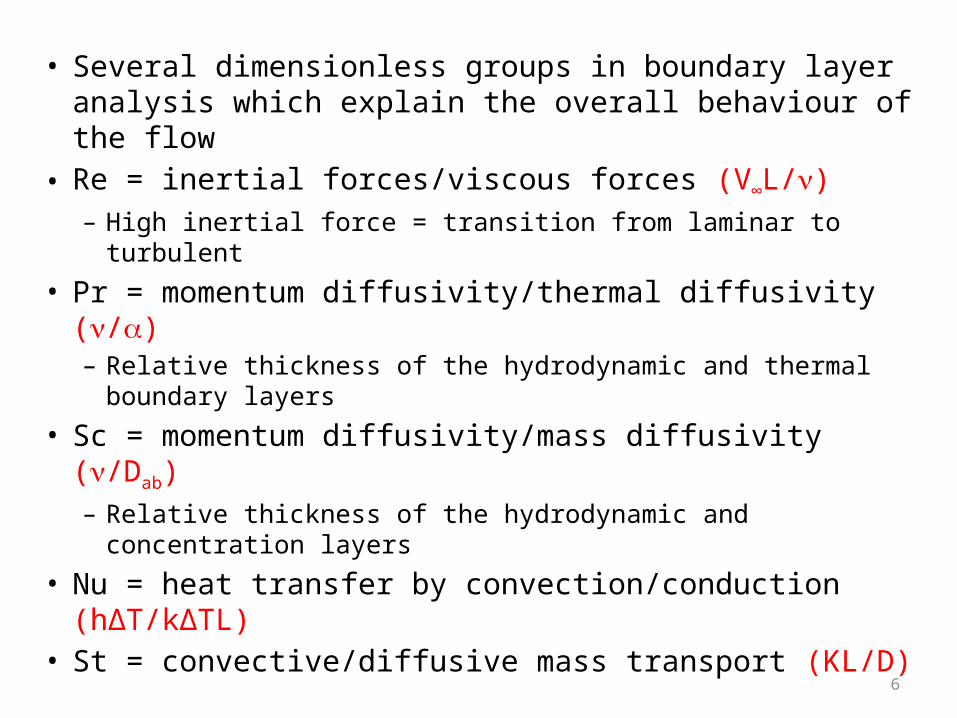
• Several dimensionless groups in boundary layer analysis which explain the overall behaviour of the flow

• Re = inertial forces/viscous forces (V∞L/)– High inertial force = transition from laminar to turbulent

• Pr = momentum diffusivity/thermal diffusivity (/)– Relative thickness of the hydrodynamic and thermal boundary

layers

• Sc = momentum diffusivity/mass diffusivity (/Dab)– Relative thickness of the hydrodynamic and concentration

layers• Nu = heat transfer by convection/conduction (hΔT/kΔTL)• St = convective/diffusive mass transport (KL/D)

7

Similar relationship can also be observed between concentration (Sc) and hydrodynamic boundary layers

hydrodynamic

Thermal

h 1/T

8

Boundary Layer Analysis• We use example of convective transport on a flat plate • By making the following assumptions:• Steady state: ( )/t = 0• Incompressible flow: ρ = constant• Constant properties: k, Dab, Cp, ρ, μ• Newtonian fluid: xy = -Vy/x, yx = -Vxy• Two dimensional flow: ( )/z = 0, Vz = 0• No energy generation: q’ = 0• No species generation: R’ = 0

9

• Continuity:

• Momentum:

• Energy:

• Mass:

0

yV

xV yx

2

2

2

21yV

xV

xP

yVV

xVV xxx

yx

x

2

2

2

21yV

xV

yP

yV

VxV

V yyyy

yx

2

2

2

2

yT

xT

yTV

xTV yx

2

2

2

2

yC

xCD

yCV

xCV aa

aba

ya

x

10

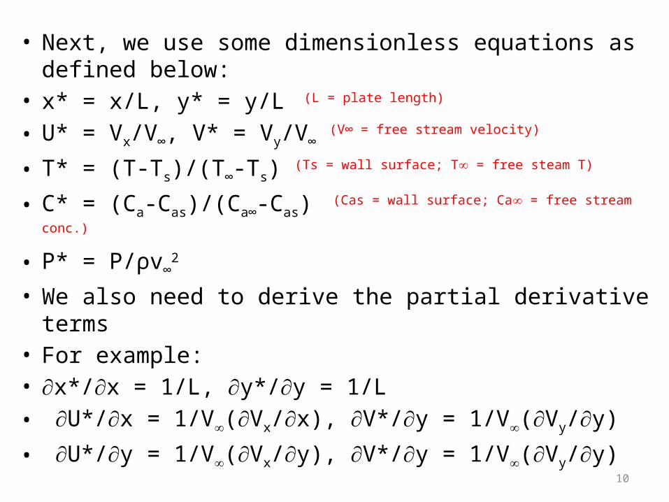
• Next, we use some dimensionless equations as defined below:

• x* = x/L, y* = y/L (L = plate length)

• U* = Vx/V∞, V* = Vy/V∞ (V∞ = free stream velocity)

• T* = (T-Ts)/(T∞-Ts) (Ts = wall surface; T = free steam T)

• C* = (Ca-Cas)/(Ca∞-Cas) (Cas = wall surface; Ca = free stream conc.)

• P* = P/ρv∞2

• We also need to derive the partial derivative terms• For example:• x*/x = 1/L, y*/y = 1/L• U*/x = 1/V(Vx/x), V*/y = 1/V(Vy/y)• U*/y = 1/V(Vx/y), V*/y = 1/V(Vy/y)

11

• The equations are transformed into dimensionless forms as below:

• Continuity:

• Momentum:

• Energy:

• Mass:

0*

*

*

*

yV

xU

2*

*2

2*

*2

*

*

*

**

*

**

Re1

yU

xU

xP

yUV

xUU

2*

*2

*2

*2

*

**

*

**

PrRe1

yT

xT

yTV

xTU

2*

*2

2*

*2

*

**

*

**

Re1

yC

xC

ScyCV

xCU

2*

*2

2*

*2

*

*

*

**

*

**

Re1

yV

xV

yP

yVV

xVU