Boundary-Value Problems for P.D.E.s

Contents: 1. P.D.E.s and boundary-value problems. 2. Elliptic equations in nondivergence form.3. Green’s formulae and related trace theorems. 4. The Fredholm alternative and the Lax-Milgramtheorem. 5. Elliptic equations in divergence form. 6. Weak solution of parabolic equations. 7.Weak solution of hyperbolic equations. 8. Finite element method

1 P.D.E.s and Boundary-Value ProblemsFor linear P.D.E.s a classification by types is well-established, at least for the second order equa-tions that are most frequently encountered in applications. At first, one distinguishes the principalpart of the differential operator, which consists of the terms that contain the highest order deriva-tives. One then speaks of elliptic, parabolic, hyperbolic operators (and equations), according tothe form of the principal part.

As it is known to the reader, typical examples of elliptic equations are the Poisson equation

−∆u = f and the equation λu − ∆u = f ; here ∆ :=∑Ni=1

∂2

∂x2i

, λ ∈ R, and f is a prescribed

function. These equations represent several stationary phenomena. The heat equation ∂u∂t −∆u =

f is parabolic equation, whereas the wave equation ∂2u∂t2 −∆u = f is hyperbolic.

This classification reflects the fact that several basic features of the qualitative behaviour ofsolutions, including the well-posedness of corresponding boundary- and/or initial-value problems,are determined by the form of the principal part, and solutions are stable with respect to largeclasses of perturbations which do not involve the principal part.

In many cases the classes of boundary conditions that make a P.D.E. well-posed are alsodetermined by the type of the equation. This, however, does not apply to parabolic equations,which indeed represent a sort of degenerate case, as the principal part corresponds to a singolarmatrix. For instance, the principal part of the heat operator a∂/∂t−∆ (with a ∈ R) is −∆; but,e.g., the well-posedness of the corresponding initial-value problem depends on the sign of a. (1)

In this section we discuss some examples of boundary-value problems for linear P.D.E.s ofsecond order of elliptic, parabolic and hyperbolic type.

Well Posedness. Following Hadamard, we say that a problem is well-posed whenever for anyset of admissible data it has one and only one solution, and this depends continuously on thedata. Obviously, this requires that data and solutions range in appropriate topological spaces.Here we briefly discuss some examples.

(i) For N = 2, let us consider the problem∂2u

∂x2+∂2u

∂y2= 0 in Ω := R×]0,+∞[,

u(x, 0) = g(x),∂u

∂y(x, 0) = 0 ∀x ∈ R,

(1.1)

with g continuous and bounded. If y is interpreted as a time variable, the two latter conditionsmay be regarded as initial conditions, and are also named Cauchy conditions. Accordingly, onespeaks of a Cauchy problem for the Laplace equation. For any n ∈ N, if gn(x) := 1

n sin(nx) forany x ∈ R, then by separation of variables one easily finds the solution

un(x, y) =1

nsin(nx) cosh(ny) ∀(x, y) ∈ R×R+. (1.2)

(1) To this purpose one might then consider an alternative notion, that besides the principal includes any

derivative Dα such that no term of the form Dβ with β > α occurs. With this convention the heat operator

would coincide with its principal part.

2

As n → ∞, gn → 0 uniformly in R, and of course u ≡ 0 solves the problem for g ≡ 0. But,as n→∞, un does not vanish uniformly in R×R+ (actually, not even in any neighbourhood ofthe straight line y = 0). Therefore this Cauchy problem is ill-posed w.r.t. the uniform topology.

On the other hand, if in (1.1) the Laplace equation is replaced by the wave equation, then theCauchy problem is well-posed w.r.t. the uniform topology. For instance, if gn is as above thenthe solution un(x, y) = 1

n sin(nx) cos(ny) vanishes uniformly as n→∞. The same applies for theheat equation (in this case a single initial condition must be prescribed, as the operator is of firstorder in time).

Let us now consider the boundary-value problem∂2u

∂x2+∂2u

∂y2= 0 in Ω := R×]0, 1[,

u(x, 0) = g(x), u(x, 1) = 0 ∀x ∈ R.

(1.3)

with g continuous and bounded. This problem is well-posed w.r.t. the uniform topology. [Ex] Forinstance, if gn(x) := 1

n sin(nx) for any x ∈ R then the solution

un(x, y) =1

n(1− e2n)sin(nx)

(eny − en(2−y)

)vanishes uniformly as n→∞.

These conclusions do not depend on the unboundedness of the domain. The above pictureis essentially unchanged in Ω :=]0, π[2, if the conditions (1.3)2 and u(0, ·) = u(π, ·) = 0 areappended. Similar conclusions apply for any N ≥ 2, and if the Laplace, wave and heat equationsare respectively replaced by general second order equations of the same type.

Boundary-Value Problems for Elliptic Equations. We introduce some boundary-valueproblems associated with the equation −∆u + u = f , which are well-posed in several classes offunction spaces. This discussion holds almost unchanged for the Poisson equation, and may beextended to more general elliptic operators. This will also provide a basis for the formulation ofinitial- and boundary-value problems for evolution equations. Here we shall just introduce theseproblems formally, i.e., without specifying the functional environment and the precise meaning ofthe equations. Regularity hypotheses and the actual well-posedness of several of these problemswill be illustrated in the next sections.

Dirichlet Condition. Let Ω be a bounded domain of RN , its boundary Γ be of class C0,1, andf : Ω → R and g : Γ → R be prescribed functions. We search for u : Ω → R such that

−∆u+ λu = f in Ω,

u = g on Γ.(1.4)

This boundary condition is named after Dirichlet, and is said of homogeneous type if g identicallyvanishes. (1.4) is then called a Dirichlet problem for the operator −∆+λI (I := identity operator)for any λ ≥ 0. If the function g is extended to the whole Ω, by setting u := u − g and f :=f +∆g − λg, the nonhomogeneous boundary condition is reduced to a homogeneous condition:

−∆u+ λu = f in Ω,

u = 0 on Γ.(1.5)

Similarly, if h : Ω → R is any function such that −∆h+λh = f in Ω, then, by setting u := u−hin Ω and g := g − h on Γ , we get a homogeneous equation coupled with a nonhomogeneousboundary condition:

−∆u+ λu = 0 in Ω,

u = g on Γ.(1.6)

3

Neumann Condition. Let Ω, Γ , f , g be as above, and let ~ν be the exterior normal unit vector onΓ . We search for u : Ω → R such that

−∆u+ λu = f in Ω,

∂u

∂~ν= g on Γ.

(1.7)

This boundary condition is named after Neumann, and is said homogeneous if g identicallyvanishes. (1.7) is then called a Neumann problem for the operator −∆+ λI.

This problem is well-posed for any λ > 0, but not for λ = 0. Indeed, under suitable regularityconditions, for λ = 0 if it has a solution then

∫Ω∆udx =

∫Γ∂u∂~ν dσ, by the Gauss-Green theorem.

This yields the compatibility condition∫Ωf dx +

∫Γg dσ = 0 on the data. Moreover, still for

λ = 0, if u is a solution then u + C is also a solution for any constant C. Thus for λ = 0 theproblem (1.7) has a solution only if it has an infinity of solutions. This is an example of a moregeneral result, known as the Fredholm alternative, which we shall address ahead.

Robin Condition. Let Ω, Γ , ~ν, f , g be as above, and a : Γ → R+. We search for u : Ω → R suchthat

−∆u+ λu = f in Ω,

∂u

∂~ν+ au = g on Γ.

(1.8)

This boundary condition is named after Robin, or after Newton, since this includes Newton’scooling law ∂u

∂~ν + a(u − u∗) = 0; here u represents the temperature and u∗ is an exterior value.This is also labelled as a condition of the third type, as sometimes the Dirichlet and the Neumannconditions are respectively named conditions of the first and second type.

Periodicity Condition. If the domain is a product of intervals:

Ω :=]a1, b1[×...×]aN , bN [ (ai < bi, ∀i),

we may search for u : Ω → R such that−∆u+ u = f in Ω,

u|xi=ai = u|xi=bi ,∂u

∂xi

∣∣∣xi=ai

=∂u

∂xi

∣∣∣xi=bi

(i = 1, ..., N).(1.9)

This is equivalent to prescribing the equation on an N -dimensional torus.

Mixed Boundary Conditions. Let Ω, Γ , ~ν, λ be as above, and Γ0, Γ1 be two nonempty opensubsets of Γ such that Γ = Γ0 ∪ Γ1. Let f : Ω → R, g : Γ0 → R, h : Γ1 → R. The problem offinding u : Ω → R such that

−∆u+ λu = f in Ω,

u = g on Γ0,

∂u

∂~ν= h on Γ1.

(1.10)

is named a mixed Dirichlet-Neumann problem. One may also consider a mixed Dirichlet-Robinproblem, or a mixed Neumann-Robin problem.

Free Space. One may also deal with the equation (1.10)1 in Ω := RN , or in other unboundeddomains. In particular, if Ω is the complement of a compact subset of RN , one speaks ofan exterior problem. Which natural boundary conditions may be prescribed in this case? Inthe following sections we shall see that integrability plays an important role in the analysis ofP.D.E.s, as several methods assume that data and certain derivatives of solutions vary in Lp-spaces(1 ≤ p < +∞). Of course, integrability in an unbounded domain suggests some restrictions onthe asymptotic behaviour (although, this does not force asymptotic vanishing!). In this case one

4

may then regard the boundary conditions as implicit in the membership of the solution in someBanach spaces.

For instance, one may deal with the Dirichlet-type problem−∆u+ λu = f in Ω := RN−1×]0,+∞[,

u = g on RN−1 × 0.(1.11)

The corresponding problem for the Poisson equation is not well-posed, as it is clear in the one-dimensional case.

Boundary-Value Problems for Hyperbolic and Parabolic Equations. We introduce someevolution problems which are well-posed in several classes of function spaces. This discussionpartly extends that of the stationary equations, as the evolution operators that we consider reduceto elliptic operators under stationary conditions. We deal with the heat and wave equations, asrepresentative of parabolic and hyperbolic equations. More general evolution operators may thenbe obtained just by replacing the Laplace operator by a more general elliptic operator, and thefollowing discussion partly extends to that setting.

Free Space. Let Ω := RN , fix any T > 0, and set Q := Ω×]0, T [. The Cauchy problems for thewave and heat equations respectively read

∂2u

∂t2−∆u = f in Q,

u(x, 0) = u0(x),∂u

∂t(x, 0) = w0(x) in Ω,

(1.12)

∂u

∂t−∆u = f in Q,

u(x, 0) = u0(x) in Ω,(1.13)

for prescribed functions f, u0, w0.

Cauchy-Dirichlet Problem. We assume that Ω is a bounded domain of RN , and Γ is its boundary.We then fix any T > 0, and set Q := Ω×]0, T [, Σ := Γ×]0, T [. Here suitable boundary conditionsmust be coupled with the initial condition(s). For instance, the Cauchy-Dirichlet problem for theheat equation reads

∂u

∂t−∆u = f in Q,

u(x, t) = g(x, t) on Σ,

u(x, 0) = u0(x) in Ω.

(1.14)

One may also couple the Cauchy condition with a Neumann condition (Cauchy-Neumann prob-lem), or with another boundary condition. For the wave equation, a second initial condition is inorder.

The set Γ × 0 is the boundary of Ω × 0 and is also a part of the boundary of Σ. We mayfind so regular a solution that the double trace on Γ × 0 is meaningful only if the data fulfilthe compatibility condition

g(x, t) = u0(x) on Γ × 0. (1.15)

The same applies to other compatibility conditions.

Functional Framework. Different formulations may be attached to the same problem, corre-sponding to different regularity hypotheses on data and solution. We outline this issue on theDirichlet problem for the equation −∆u+ λu = f , for any λ ≥ 0.

5

Classical Formulation. This setting refers to spaces of either continuous or Holder-continuousfunctions. Here f and g are assumed to be (at least) continuous, u is required to belong toC2(Ω)∩C0(Ω); the equation and the boundary condition are then assumed to hold at all points.

Strong Formulation. Here we move to Sobolev spaces. We fix any p ∈ [1,+∞[, and assume thatΩ is at least of class C0,1, so that γ0 : W 1,p(Ω) → W 1−1/p,p(Γ ). For any f ∈ Lp(Ω) and anyg ∈W 1−1/p,p(Γ ), we search for u ∈W 1,p(Ω) such that ∆u ∈ Lp(Ω) and

−∆u+ λu = f a.e. in Ω,

γ0u = g a.e. on Γ.(1.16)

Weak Formulation. The restriction “∆u ∈ Lp(Ω)” is here removed by interpreting the equationin the sense of distributions. We assume that f ∈ W−1,p(Ω), g ∈ W 1−1/p,p(Γ ), and search foru ∈W 1,p(Ω) such that

−∆u+ λu = f in D′(Ω),

γ0u = g a.e. on Γ.(1.17)

In the analysis of these problems, usually one first deals with the weak formulation. Provingexistence of a solution is the first task; one then tries to derive its uniqueness and qualitative prop-erties. Under stronger assumptions on the data, one also tries to establish regularity propertiesof the weak solution, aiming to show that this is a strong solution, or even a classical one.

2 Elliptic Operators in Nondivergence Form

Some Classical Results for the Laplace Operator. Any function Ω → R such that ∆u = 0(∆u ≥ 0, ∆u ≤ 0, resp.) in D′(Ω) is called harmonic (subharmonic, superharmonic, resp.), forreasons that will appear clear by the results of this section. Let us denote by ωN the measure ofthe unit ball of RN , so that the (N − 1)-dimensional measure of the corresponding unit sphere isNωN .

Theorem 2.1 (Mean Value Principle) Let Ω be a domain of RN (N ≥ 1) and u ∈ C2(Ω).Then ∆u ≥ 0 in Ω iff

u(x) ≤ 1

NωNRN−1

∫∂B(x,R)

u(y) dσ(y)(

=1

NωN

∫∂B(0,1)

u(x+Ry) dσ(y))

∀R > 0 such that B(x,R) ⊂ Ω, ∀x ∈ Ω.(2.1)

Proof. If ∆u ≥ 0 in Ω, then by the Gauss-Green theorem we have

0 ≤∫B(x,R)

∆u(y) dy =

∫∂B(x,R)

∂u

∂~ν(y) dσ(y) = RN−1

∫∂B(0,1)

∂u

∂R(x+Ry) dσ(y)

= RN−1 d

dR

∫∂B(0,1)

u(x+Ry) dσ(y).

Therefore the function

ϕx : R 7→ 1

NωN

∫∂B(0,1)

u(x+Ry) dσ(y) =1

NωNRN−1

∫∂B(x,R)

u(y) dσ(y)

is nondecreasing. As ϕx(R)→ u(x) as R→ 0+, (1) follows.We prove the converse statement by contradiction. If ∆u(x) < 0 for some x ∈ Ω, then by

continuity ∆u < 0 in an open subset of Ω. By the above argument, ϕx is then strictly decreasingin a neighbourhood of R = 0, and (2.1) fails. tu

6

This theorem has several important consequences.

Corollary 2.2 Let Ω be a domain of RN (N ≥ 1) and u ∈ C2(Ω). Then ∆u ≥ 0 in Ω iff

u(x) ≤ 1

ωNRN

∫B(x,R)

u(y) dy ∀R > 0 such that B(x,R) ⊂ Ω, ∀x ∈ Ω. (2.2)

Proof. This is easily checked multiplying (2.1) by NωNRN−1 and integrating w.r.t. R. tu

Corollary 2.3 Let Ω be a domain of RN (N ≥ 1), and u ∈ C2(Ω). Then ∆u = 0 in Ω iffeither of the following properties holds

u(x) =1

NωNRN−1

∫∂B(x,R)

u(y) dσ(y) ∀R > 0 such that B(x,R) ⊂ Ω, ∀x ∈ Ω, (2.3)

u(x) =1

ωNRN

∫B(x,R)

u(y) dy ∀R > 0 such that B(x,R) ⊂ Ω, ∀x ∈ Ω. (2.4)

Corollary 2.4 (Strong Maximum Principle) Let Ω be a domain of RN (N ≥ 1), and u ∈ C2(Ω).If ∆u ≥ 0 in Ω, then either u is constant, or u(x) < supΩ u for any x ∈ Ω.

Proof. We can assume that S := supΩ u < +∞. By continuity of u, A := x ∈ Ω : u(x) = S isa closed subset of Ω, and by (2.4) it is open. Therefore either A = Ω or A = ∅. tu

Let now Ω be a bounded domain of RN . For any subharmonic function u ∈ C2(Ω) ∩ C0(Ω),the strong maximum principle entails the weaker inequality u(x) ≤ supΓ u. This is known as theweak maximum principle, and entails the following properties: (2)

(i) The solution depends monotonically on the interior and boundary data. That is, assumingthat u1, u2 ∈ C2(Ω) ∩ C0(Ω),

if −∆u1 ≤ −∆u2 in Ω and u1 ≤ u2 on Γ , then u1 ≤ u2 in Ω.

(ii) The solution depends continuously on the boundary datum w.r.t. to the uniform topology.That is, assuming that u1, u2 ∈ C2(Ω) ∩ C0(Ω),

if −∆u1 = −∆u2 in Ω then maxΩ |u1 − u2| ≤ maxΓ |u1 − u2|.

(iii) The solution of the Dirichlet problem for the Poisson equation −∆u = f is unique.The weak maximum principle is also at the basis of the following classical result (which can

also be stated under weaker regularity hypotheses on Ω).

Theorem 2.5 (Perron) Let Ω be a bounded domain of RN of class C2, g ∈ C0(Γ ), and set

Sg := v ∈ C0(Ω) : −∆v ≤ 0 in D′(Ω), v ≤ g on Γ, u(x) := maxv∈Sg

v(x) ∀x ∈ Ω. (2.5)

Then u ∈ C0(Ω) and

∆u = 0 in D′(Ω), u = g on Γ. [] (2.6)

Analogous results can be stated for superharmonic functions; in this case one derives minimumprinciples.

(2) Despite of the terminology, the strong and weak maximum principles have no relation with the conceptsof strong and weak solution.

7

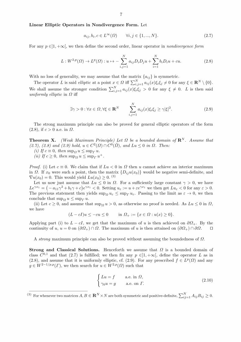
Linear Elliptic Operators in Nondivergence Form. Let

aij , bi, c ∈ L∞(Ω) ∀i, j ∈ 1, ..., N. (2.7)

For any p ∈]1,+∞[, we then define the second order, linear operator in nondivergence form

L : W 2,p(Ω)→ Lp(Ω) : u 7→ −N∑

i,j=1

aijDiDju+N∑i=1

biDiu+ cu. (2.8)

With no loss of generality, we may assume that the matrix aij is symmetric.

The operator L is said elliptic at a point x ∈ Ω iff∑Ni,j=1 aij(x)ξiξj 6= 0 for any ξ ∈ RN \ 0.

We shall assume the stronger condition∑Ni,j=1 aij(x)ξiξj > 0 for any ξ 6= 0. L is then said

uniformly elliptic in Ω iff

∃γ > 0 : ∀x ∈ Ω, ∀ξ ∈ RNN∑

i,j=1

aij(x)ξiξj ≥ γ|ξ|2. (2.9)

The strong maximum principle can also be proved for general elliptic operators of the form(2.8), if c > 0 a.e. in Ω.

Theorem X. (Weak Maximum Principle) Let Ω be a bounded domain of RN . Assume that(2.7), (2.8) and (2.9) hold, u ∈ C2(Ω) ∩ C0(Ω), and Lu ≤ 0 in Ω. Then:

(i) If c ≡ 0, then supΩ u ≤ supΓ u.(ii) If c ≥ 0, then supΩ u ≤ supΓ u

+.

Proof. (i) Let c ≡ 0. We claim that if Lu < 0 in Ω then u cannot achieve an interior maximumin Ω. If x0 were such a point, then the matrix Diju(x0) would be negative semi-definite, and∇u(x0) = 0. This would yield Lu(x0) ≥ 0. (3)

Let us now just assume that Lu ≤ 0 in Ω. For a sufficiently large constant γ > 0, we haveLeγx1 =

(− a11γ

2 + b1γ+ c)eγx1 < 0. Setting uε := u+ εeγx1 we then get Luε < 0 for any ε > 0.

The previous statement then yields supΩ uε ≤ supΓ uε. Passing to the limit as ε → 0, we thenconclude that supΩ u ≤ supΓ u.

(ii) Let c ≥ 0, and assume that supΩ u > 0, as otherwise no proof is needed. As Lu ≤ 0 in Ω,we have

(L− cI)u ≤ −cu ≤ 0 in Ω+ := x ∈ Ω : u(x) ≥ 0.

Applying part (i) to L − cI, we get that the maximum of u is then achieved on ∂Ω+. By thecontinuity of u, u = 0 on (∂Ω+) ∩Ω. The maximum of u is then attained on (∂Ω+) ∩ ∂Ω. tu

A strong maximum principle can also be proved without assuming the boundedness of Ω.

Strong and Classical Solutions. Henceforth we assume that Ω is a bounded domain ofclass C0,1 and that (2.7) is fulfilled; we then fix any p ∈]1,+∞[, define the operator L as in(2.8), and assume that it is uniformly elliptic, cf. (2.9). For any prescribed f ∈ Lp(Ω) and anyg ∈W 2−1/p,p(Γ ), we then search for u ∈W 2,p(Ω) such that

Lu = f a.e. in Ω,

γ0u = g a.e. on Γ.(2.10)

(3) For whenever two matricesA,B ∈ RN×N are both symmetric and positive-definite,∑Nij=1 AijBij ≥ 0.

8

A result analogous to Perron’s Theorem 2.5 holds for problem (2.10), with L in place of −∆.(The elements of Sg are here named subsolutions.) []

The following two classical results may be derived either via potential theory, or via Banachspace interpolation.

* Theorem 2.6 (Agmon-Douglis-Nirenberg) Let k ∈ N0, Ω be a bounded domain of classCk+1,1, and 1 < p < +∞. Moreover, let aij , bi, c ∈W k,∞(Ω) for any i, j, c ≥ 0 a.e., and L be asin (2.8). Then:

(i) For any f ∈W k,p(Ω) and g ∈W k+2−1/p,p(Γ ), there exists a unique solution u ∈W k+2,p(Ω)of problem (2.10).

(ii) There exists a constant Ck > 0 such that

‖v‖Wk+2,p(Ω) ≤ Ck(‖Lv‖Wk,p(Ω) + ‖γ0v‖Wk+2−1/p,p(Γ )

)∀v ∈W k+2,p(Ω). [] (2.11)

* Theorem 2.7 (Schauder) Let k ∈ N0, 0 < α < 1, and Ω be a bounded domain of classCk+2,α. Moreover, let aij , bi, c ∈ Ck,α(Ω) for any i, j, c ≥ 0 a.e., and L be as in (2.8). Then:

(i) For any f ∈ Ck,α(Ω) and g ∈ Ck+2,α(Ω), then there exists a unique solution u ∈ Ck+2,α(Ω)of problem (2.10).

(ii) There exists a constant Ck > 0 such that

‖v‖Ck+2,α(Ω) ≤ Ck(‖Lv‖Ck,α(Ω) + ‖v‖Ck+2,α(Γ )

)∀v ∈ Ck+2,α(Ω). [] (2.12)

If N > 1, for α = 0 Theorem 2.7 fails. For either theorem, if the hypothesis c ≥ 0 is dropped,then a Fredholm alternative applies, see ahead.

Finally, as a simple consequence of part (i) of the latter theorem, for any f, g ∈ C∞(Ω), thereexists a unique solution u ∈ C∞(Ω) of problem (2.10).

3 The Green Formula and Related Trace ResultsIn view of the analysis of weak formulations, we need an extension of the formula of partial

integration to several dimensions. This will also provide some further trace theorems. We stillassume that Ω is a domain of RN and denote its boundary by Γ .

Theorem 3.1 (Classical Green’s Formulae for the Laplace Operator) Let Ω be bounded domainof class C0,1, and ~ν be the exterior normal unit vector on Γ . Then

−∫Ω

(∆u)v dx =

∫Ω

∇u · ∇v dx−∫Γ

∂u

∂~νv dσ ∀u ∈ C2(Ω),∀v ∈ C1(Ω), (3.1)

∫Ω

[(∆v)u− (∆u)v] dx =

∫Γ

(∂v∂~νu− ∂u

∂~νv)dσ ∀u, v ∈ C2(Ω). (3.2)

Proof. The classical Gauss theorem reads∫Ω

∇ · ~z dx =

∫Γ

~z · ~ν dσ ∀~z ∈ C1(Ω)N (∇· := div), (3.3)

and taking ~z := v ~w we get the following extension of the formula of partial integration to severaldimensions∫

Ω

(∇v) · ~w dx+

∫Ω

v∇ · ~w dx =

∫Γ

v ~w · ~ν dσ ∀~w ∈ C1(Ω)N ,∀v ∈ C1(Ω). (3.4)

The choice ~w := ∇u then yields the first Green formula (3.1). By exchanging u and v andsubtracting the two formulas, we then get the second Green formula (3.2). tu

9

Green’s Function. The second Green formula allows us to transform the Dirichlet problem asfollows. Let E ∈ D′(RN ) be a fundamental solution of the operator −∆ (4) For any y ∈ Ω, letw(x, y) (we do not specify its regularity) be such that

−∆xw(x, y) = 0 ∀x ∈ Ω,w(x, y) = E(x− y) ∀x ∈ Γ.

(3.5)

In general it is not easier to solve this problem rather than (2.10); however, in presence of specialsymmetries, this problem may be solved explicitly. The second Green formula (3.2) then yields

−∫Ω

(∆xu(x))w(x, y) dx =

∫Γ

(∂w∂~ν

(x, y)u(x)− ∂u

∂~ν(x)w(x, y)

)dσ(x). (3.6)

(Here and below, the normal derivative ∂∂~ν acts on the variable x.) Setting

G(x, y) := E(x− y)− w(x, y) for a.a. (x, y) ∈ Ω,

we get −∆xG(x, y) = δy in D′(Ω)

G(x, y) = 0 ∀x ∈ Γ∀y ∈ Ω. (3.7)

Although G 6∈ C2(Ω), taking v(x) := G(x, y) a formal application of (3.2) yields

u(y) = 〈δy, u〉 = 〈∆xG(x, y), u(x)〉

=

∫Ω

G(x, y)∆xu(x) dx+

∫Γ

∂G

∂~ν(x, y)u(x) dσ(x) ∀u ∈ C2(Ω).

(3.8)

Therefore the solution of the (nonhomogeneous) Dirichlet problem (2.10) reads

u(y) =

∫Ω

G(x, y)f(x) dx+

∫Γ

∂G

∂~ν(x, y)g(x) dσ(x). (3.9)

G is named the Green function relative to −∆ in the domain Ω.This classical procedure allows one to exhibit explicit solutions for special geometries (e.g.,

a ball, a half-plane, and so on). However here we intend to make a different use of the Greenformula.

Normal Traces. Let Ω be a domain of RN of class C0,1, and set

L2div(Ω)N := ~v ∈ L2(Ω)N : ∇ · ~v ∈ L2(Ω), (3.10)

which is a Banach space equipped with the graph norm

‖~v‖L2div

(Ω)N :=(‖~v‖2L2 + ‖∇ · ~v‖2L2

)1/2. (3.11)

Lemma 3.2 If Ω be a domain of RN of class C0,1, then the space D(Ω)N is dense in L2div(Ω)N .

[]

Theorem 3.3 (Normal Traces) Let Ω be a bounded domain of RN of class C0,1.(i) There exists a unique linear and continuous trace operator γν : L2

div(Ω)N → H−1/2(Γ )

(4) We remind the reader that E ∈ D′(RN ) is called a fundamental solution the differential operator L

whenever LE = δ0 (the Dirac measure at the origin) in D′(RN ).

10

such that, denoting by 〈·, ·〉 the duality pairing between H1/2(Γ ) and H−1/2(Γ ), the followinggeneralized formula of partial integration holds

−∫Ω

(∇ · ~u)v dx =

∫Ω

~u · ∇v dx− 〈∂~u∂~ν, v〉 ∀~u ∈ L2

div(Ω)N ,∀v ∈ D(Ω). (3.12)

(ii) There exists a (nonunique) linear and continuous lift operator Rν : H−1/2(Γ )→ L2div(Ω)N

such that γνRνv = v for any v ∈ H−1/2(Γ ). []

Proof. By (3.4) and by the continuity of the lift operator R : H1/2(Γ ) → H1(Ω), there existconstants C1, C2 > 0 such that∣∣∣ ∫

Γ

v ~w · ~ν dσ∣∣∣ ≤ C1‖~w‖L2

div(Ω) ‖v‖H1(Ω) ≤ C2‖~w‖L2

div(Ω) ‖γ0v‖H1/2(Γ )

∀~w ∈ D(Ω)N ,∀v ∈ H1(Ω).

By the density lemma, the operator D(Ω)N → D(Γ ) : ~w 7→ ~w · ~ν can then be extended bycontinuity to an operator L2

div(Ω)N → H1/2(Γ )′ (= H−1/2(Γ )). Therefore the generalized formulaof partial integration (3.12) holds.

In order to prove the converse, let us now fix any g ∈ H−1/2(Γ ), and notice that the mappingFg : v 7→ 〈g, v〉 is an element of H1(Ω)′. By Theorem 5.1 (see later on), for any large enoughconstant λ, there exists one and only one u ∈ H1(Ω) such that

−∫Ω

(∇u · ∇v + λuv) dx = Fg(v)(= −〈g, v〉) ∀v ∈ H1(Ω), (3.13)

and the mapping H1(Ω)′ → H1(Ω) : Fg 7→ u is continuous. The same then holds for the mappingH−1/2(Γ )→ L2

div(Ω)N : g 7→ ∇u.By the Green formula (3.12) we conclude that γνRνv = v for any v ∈ H−1/2(Γ ). tu

Second Order Elliptic Operators in Divergence Form.Let

aij , bj , ci, d ∈ L∞(Ω) ∀i, j ∈ 1, ..., N, (3.14)

and define the second order, linear operator in divergence form

L : H1(Ω)→ H−1(Ω) : u 7→ −N∑j=1

Dj

( N∑i=1

aijDiu+ bju

)+

N∑i=1

ciDiu+ du, (3.15)

and the formal adjoint operator

L∗ : H1(Ω)→ H−1(Ω) : v 7→ −N∑i=1

Di

( N∑j=1

aijDjv + civ

)+

N∑j=1

bjDjv + dv. (3.16)

We shall see that ∫Ω

vLu dx =

∫Ω

uL∗v dx ∀v ∈ H10 (Ω), (3.17)

which explains the denomination we used for L∗.(Here we confine ourselves to p = 2, since the most important results are known for this

setting.) Ellipticity and uniform ellipticity are here defined as above. If the coefficients aresufficiently regular, it is easy to see that any operator in divergence form can also be representedin nondivergence form, and conversely. Moreover, any operator in divergence form is elliptic(uniform elliptic, resp.) iff the same holds for the equivalent operator in nondivergence form.

11

The next result can be proved by an argument similar to that of Theorem 3.1.

Theorem 3.4 (Classical Green’s Formulae for Operators in Divergence Form) Let Ω be abounded domain of RN of class C0,1, Γ be its boundary, and ~ν be the exterior normal unitvector on Γ . Then

−∫Ω

vLu dx =

∫Ω

( N∑i,j=1

aijDiuDjv +

N∑j=1

bjuDjv +

N∑i=1

ci(Diu)v + duv

)dx

−∫Γ

v

N∑j=1

( N∑i=1

aijDiu+ bju

)νj dσ ∀u ∈ C2(Ω),∀v ∈ C1(Ω),

(3.18)

∫Ω

[vLu− uL∗v] dx =

∫Γ

vN∑j=1

( N∑i=1

aijDiu+ bju

)νj dσ

−∫Γ

uN∑i=1

( N∑j=1

aijDjv + civ

)νi dσ ∀u, v ∈ C2(Ω).

(3.19)

(3.17) then follows, by a density argument.

Conormal Traces. Let L be defined as in (3.15), and set

H1L(Ω)N := v ∈ H1(Ω) : Lv ∈ L2(Ω). (3.20)

This is a Banach space equipped with the graph norm

‖v‖H1L

(Ω) :=(‖v‖2H1 + ‖Lv‖2L2

)1/2

. (3.21)

Theorem 3.5 (Conormal Traces) Let Ω be a bounded domain of RN of class C0,1, and theoperator L be defined as in (3.15).

(i) There exists a unique linear and continuous operator γL : H1L(Ω)→ H−1/2(Γ ) such that

−∫Ω

vLu dx =

∫Ω

( N∑i,j=1

aijDiuDjv +N∑j=1

bjuDjv +N∑i=1

ci(Diu)v + duv

)dx

− 〈γLu, v〉 ∀u ∈ D(Ω),∀v ∈ H1(Ω),

(3.22)

(ii) There exists a (nonunique) linear and continuous lift operator RL : H−1/2(Γ )→ H1L(Ω)N

such that γLRL~v = v for any ~v ∈ H−1/2(Γ ). []

By generalized partial integration γLu =∑Ni,j=1(aijDiu+ bjuv)νj .

Proof. This is analogous to that of Thereom 3.3. tu

12

4 The Fredholm Alternative and the Lax-Milgram Theorem

NOTE: Theorems 4.1 and 4.2 have been skipped this year......

Theorem 4.1 (Riesz-Schauder) Let B be a Banach space and T ∈ L(B) be a compact operator.(5) Then:

(i) R(I − T ) = N(I − T ∗)⊥;(ii) dim N(I − T ) = dim N(I − T ∗) < +∞. []

As for part (i), the point is that R(I − T ) is closed, as one can prove that R(A) = N(A∗)⊥ forany A ∈ L(B). [] (The inclusion R(A) ⊂ N(A∗)⊥ is straightforward, for one easily checks thatN(A∗) ⊂ R(A)⊥.)

For part (ii) the point is that N(I − T ) and N(I − T ∗) have the same dimension, as by thecompactness of T it is clear that both are finite dimensional.

In terms of the Fredholm theory, Theorem 4.1 entails that I − T has null Fredholm index

Ind(I − T ) := dim N(I − T )− codim R(I − T ).

In fact

codim R(I − T ) = dim R(I − T )⊥ = (by (i)) dim N(I − T ∗) = (by (ii)) dim N(I − T ).

Notice that by (i)R(I − T ) = B ⇔ N(I − T ) = 0;

namely, the operator I − T is surjective iff it is injective. In this case (I − T )−1 ∈ L(B) (e.g., bythe closed graph theorem). The following statement is more precise.

Corollary 4.2 (“Existence ⇔ Uniqueness”) Let B be a Banach space and T ∈ L(B) be acompact operator.

(i) If Tw = w only for w = 0, then the equation u− Tu = f has a (unique) solution u for anyf ∈ B, and the mapping B → B : f 7→ u is continuous.

(ii) If Tw = w for some w 6= 0, then the equation u− Tu = f has a (nonunique) solution u iff

B〈f, v〉B′ = 0 ∀v ∈ B′ : T ∗v = v. (4.1)

Moreover, these functions v span a finite dimensional vector space. Furthermore, denoting byP the operator that selects the minimal norm element, the operator P (I − T )−1 is continuousin B; that is, there exists a constant C > 0 such that

inf‖v‖B : v = Tv ≤ C‖v‖B ∀v ∈ B. (4.2)

Thus there are two alternatives:(i) either the equation u− Tu = f has one and only one solution for any f ∈ B,(ii) or it has a (nonunique) solution iff f fulfils a finite number of orthogonality conditions,

cf. (4.1).This extends what is already known for linear systems in RN , Au = f . Indeed, for any linear

operator A in RN , T := I −A is trivially compact.Here the hypothesis of compactness is essential. E.g., in `2 the left (right, resp.) shift: s` :

(u1, u2, ...) → (u2, u3, ...) (sr : (u1, u2, ...) → (0, u1, u3, ...), resp.) are linear and continuous, butthe operator I − s` (I − sr, resp.) is noncompact. The mapping s` is surjective but noninjective,whereas sr is injective but nonsurjective.

(5) This means that T (S) is compact for any bounded set S ⊂ B.

13

Theorem 4.3 (Lax-Milgram) Let H be a Hilbert space, and A ∈ L(H) be such that, for someα > 0,

(Av, v) ≥ α‖v‖2 ∀v ∈ H (coerciveness). (4.3)

Then A is bijective, and ‖A−1f‖ ≤ α−1‖f‖ for any f ∈ H.

Proof. The coerciveness yields α‖v‖2 ≤ (Av, v) ≤ ‖Av‖‖v‖ for any v ∈ H, whence α‖v‖ ≤ ‖Av‖.This entails that A is injective, and, for any sequence vn in H, that Avn is a Cauchy sequenceonly if the same holds for vn. By the continuity of A, A(H) is then a closed vector subspace ofH.

For any v ∈ A(H)⊥, we have α‖v‖2 ≤ (Av, v) = 0, whence v = 0. Therefore A(H) = H. Theboundedness of A−1 then follows from the stated inequality α‖v‖ ≤ ‖Av‖ for any v ∈ H. tu

This theorem generalizes the Riesz-Frechet representation Theorem IV.1.9 to nonsymmetricoperators. We check this assuming that H is a real Hilbert space, for the sake of simplicity. If(Au, v) = (Av, u) for any u, v ∈ H, then (u, v) 7→ ((u, v)) := (Au, v) is a scalar product over H;moreover, by the continuity and coerciveness of A, the corresponding norm is equivalent to theoriginal one. Then, by the representation theorem, for any f ∈ H ′ setting u := R−1f ∈ H wehave ((u, v)) = 〈f, v〉 for any v ∈ H, i.e., Au = f .

5 Elliptic Equations in Divergence FormHenceforth we assume that Ω is a bounded domain of class C0,1 and that (3.14) is fulfilled; we

then define L as in (3.15), and assume that it is uniformly elliptic, cf. (2.9). For any prescribedf ∈ H−1(Ω), any g ∈ H1/2(Γ ) and any parameter λ ∈ R, we then search for u ∈ H1(Ω) suchthat

Lu+ λu = f in H−1(Ω),

γ0u = g a.e. on Γ.(5.1)

For some purposes it is convenient to transform this problem to a homogeneous Dirichletproblem. Let R ∈ L

(H1/2(Γ );H1(Ω)

)be a lift operator. By setting f := f − LRg − λRg and

u := u−Rg, (5.1) equivalently readsLu+ λu = f in H−1(Ω),

γ0u = 0 a.e. on Γ (i.e., u ∈ H10 (Ω)).

(5, 2)

Theorem 5.1 (Well-Posedness) Let Ω be a bounded domain of class C0,1, (3.14) be fulfilled, Lbe as in (3.15), and uniformly elliptic. Then there exists λ ∈ R such that, for any λ ≥ λ:

(i) For any f ∈ H−1(Ω) and any g ∈ H1/2(Γ ), there exists a unique solution u ∈ H1(Ω) ofproblem (5.1).

(ii) There exists a constant C > 0 such that

‖u‖H1(Ω) ≤ C(‖Lu‖H−1(Ω) + ‖γ0u‖H1/2(Γ )

)∀u ∈ H1(Ω). (5.3)

Proof. Let us consider the homogeneous problem (5.2). If λ is large enough, the linear andcontinuous operator L + λI : H1

0 (Ω) → H−1(Ω) is coercive. [Ex] By the Lax-Milgram Theorem

4.3, this operator is then bijective, and ‖u‖H10 (Ω) ≤ α−1‖f‖H−1(Ω). In terms of the solution u of

the corresponding problem (5.1), this reads

‖u−Rg‖H10 (Ω) ≤ α−1‖f − LRg − λRg‖H−1(Ω).

As‖LRg − λRg‖H−1(Ω) ≤ ‖Rg‖H1(Ω) ≤ ‖g‖H1/2(Γ )

14

we then get (5.3). tu

Theorem 5.2 (Fredholm Alternative) Let Ω be a bounded domain of class C0,1, (3.14) befulfilled, L be as in (3.15), and uniformly elliptic. Let λ ∈ R and f ∈ H−1(Ω). Then there existsa finite dimensional subspace F of H1

0 (Ω) such that problem (5.2) has a solution u iff 〈f, v〉 = 0for any v ∈ F . Moreover, F 6= 0 only for a discrete family of λs (with λ < λ). Finally, thereexists a constant C > 0 such that

inf‖u‖H1

0 (Ω) : (5.1) holds≤ C

(‖f‖H−1(Ω) + ‖g‖H1/2(Γ )

)∀f ∈ H−1(Ω),∀g ∈ H1/2(Γ ).

(5.4)

Proof. Let us define λ as in Theorem 5.1, and denote by J the canonic imbedding H10 (Ω) →

H−1(Ω). The operator T := J (L + λI)−1 is then a linear and compact operator in H−1(Ω).Henceforth we shall omit the operator J . The equation (5.1)1 also reads (L+λI)u = f+(λ−λ)u =:w, namely, u = Tw. In terms of w this equation is also equivalent to

w − (λ− λ)Tw = f in H−1(Ω).

By the Fredholm alternative, cf. Theorem 4.2, this problem has a solution iff

(f, z)H−1(Ω) = 0 ∀z ∈ H−1(Ω) such that z = (λ− λ)T ∗z.

By the compactness of T , the latter equality just holds for an at most countable number ofisolated λ < λ.

Notice also that (f, z)H−1(Ω) = 〈f, v〉 if v ∈ H10 (Ω) is such that ∆v = z in D′(Ω). Setting

F := v ∈ H10 (Ω) : ∆v = (λ− λ)T ∗∆v, we thus get

〈f, v〉 = 0 ∀v ∈ F.

tu

Theorem 5.3 (Regularity) Let k ∈ N0, Ω be a bounded domain of class Ck+2, L be as in (3.15)and uniformly elliptic, aij , bj ∈W k+1,∞(Ω) and ci, d ∈W k,∞(Ω) for any i, j. Then:

(i) For any u ∈ H1(Ω), if Lu ∈ Hk(Ω) and γ0u ∈ Hk+3/2(Γ ), then u ∈ Hk+2(Ω).(ii) There exists a constant Ck > 0 such that

‖u‖Hk+2(Ω) ≤ Ck(‖Lu‖Hk(Ω) + ‖γ0u‖Hk+3/2(Γ )

)∀u ∈ Hk+2(Ω).

[]

As a simple consequence of part (i) of the latter theorem, for any u ∈ H1(Ω), if Lu ∈ C∞(Ω)and γ0u ∈ C∞(Ω), then u ∈ C∞(Ω).

Theorem 4 (Weak Maximum Principle) Let k ∈ N0, Ω be a bounded domain of class Ck+2,L be as in (3.15) and uniformly elliptic, with bj = ci = 0 for any i, j and d > 0. Then, for anyu ∈ H1(Ω) such that Lu ∈ L1

loc(Ω):(i) If Lu ≤ 0 a.e. in Ω, then

u ≤ max

ess supΩ

Lu

d, ess sup

Γγ0u

=: M a.e. in Ω.

(ii) If Lu ≥ 0 a.e. in Ω, then

u ≥ min

ess infΩ

Lu

d, ess inf

Γγ0u

=: m a.e. in Ω.

15

(Both m = −∞ and M = +∞ are not excluded.)

Proof. Obviously, it suffice to prove part (i). With no loss of generality, we may assume that Mis finite. Let us multiply Lu by (u−M)+ (∈ H1

0 (Ω)). We have

DjuDi(u−M)+ = Dj(u−M)Di(u−M)+ = Dj(u−M)+Di(u−M)+ a.e. in Ω, ∀i, j,

and du(u−M)+ ≥ 0 a.e. in Ω. Hence

a

∫Ω

|∇(u−M)+|2 dx ≤N∑

i,j=1

∫Ω

aijDj(u−M)+Di(u−M)+ dx

≤ 〈Lu− du, (u−M)+〉 ≤ 0.

We then conclude that (u−M)+ = 0 a.e. in Ω. tu

The hypotheses of the latter theorem might be weakened. Under these hypotheses, one mightalso prove a strong maximum principle:

if u ∈ H1(Ω) and, for some ball B ⊂⊂ Ω, ess supB v = ess supΩ v < +∞, then u is a.e.constant in Ω. []

* Theorem 5. (L∞-Bound and De Giorgi-Nash) Let L be as above, u ∈ H1(Ω) be such thatLu = f1 +∇ · f2 with f1 ∈ Lp(Ω), f2 ∈ L2p(Ω) for some p > N . [Hence f1 +∇ · f2 ∈ H−1(Ω).]Then u ∈ L∞(Ω) ∩ C0,α(Ω). Moreover, there exist constants C > 0 and CΩ′ > 0 (for anyΩ′ ⊂⊂ Ω) such that, for any f1 ∈ Lp(Ω) and any f2 ∈ L2p(Ω),

‖u‖L∞(Ω) ≤ C(‖u‖L2(Ω) + ‖f1‖Lp(Ω) + ‖f2‖L2p(Ω)

),

‖u‖C0,α(Ω′) ≤ CΩ′(‖u‖L2(Ω) + ‖f1‖Lp(Ω) + ‖f2‖L2p(Ω)

).

[]

The Galerkin Method.

Lemma X. Let Ω be a bounded domain of class C0,1, L be as in (3.15), symmetric and uniformlyelliptic. Then there a exists a countable orthonormal basis wn of L2(Ω) which consists ofeigenvectors of L. The associated sequence of eigenvalues λn ⊂ R+ diverges.

For any m ∈ N, let Vm be the subspace of L2(Ω) spanned by λn : n = 1, ...,m. Let us setam := (f, wm), um :=

∑mn=1 λ

−1n anwn, and fm :=

∑mn=1 anwn. Then Lum = fm in V ′m, and

um → u in V .

6 Variational Techniques of L2-Type

In this section we outline the variational approach to two simple initial- and boundary-valueproblems for the heat equation and for the wave equation, resp., in the framework of Sobolevspaces of Hilbert type.

Let Ω be a bounded domain of RN (N ≥ 1) of class C0,1. We denote its boundary by Γ ,

fix any T > 0 and set Q := Ω×]0, T [, Σ := Γ×]0, T [. As above, we set ∆ :=∑Ni=1

∂2

∂x2i

. We

assume that f1 : Q → R, u0, w0 : Ω → R are prescribed functions, and deal with the followingCauchy-Dirichlet problems

∂u

∂t−∆u = f1 in Q,

u = 0 on Σ,

u(·, 0) = u0 in Ω,

(6.1)

16∂2u

∂t2−∆u = f1 in Q,

u = 0 on Σ,

u(·, 0) = u0,∂u

∂t(·, 0) = w0 in Ω.

(6.2)

We set V := H10 (Ω) and H := L2(Ω), and identify H with its topological dual H ′. As the

injection V → H is continuous and dense, in turn H ′ can be identified with a subspace of V ′.This yields the Hilbert triplet V ⊂ H = H ′ ⊂ V ′, with dense injections. We denote by V ′〈·, ·〉Vthe duality pairing between V ′ and V , and define the operator

A ∈ L(V ;V ′), V ′〈Au, v〉V :=

∫Ω

∇u · ∇v dx ∀u, v ∈ V.

Hence Av = −∆v in D′(Ω), and, after an obvious identification, A : L2(0, T ;V ) → L2(0, T ;V ′)is linear and continuous.

Weak Formulation of the Heat Equation. We assume that

u0 ∈ H, f ∈ L2(0, T ;V ′), (6.3)

and introduce a weak formulation of (6.1).

Problem 6.1 To find u ∈ L2(0, T ;V ) such that∫∫Q

(− u∂v

∂t+∇u · ∇v

)dxdt =

∫ T

0V ′〈f, v〉V dt+

∫Ω

u0v(·, 0) dx

∀v ∈ H1(0, T ;H) ∩ L2(0, T ;V ), v(·, T ) = 0.

(6.4)

Interpretation. (6.4) yields

∂u

∂t+Au = f in L2(0, T ;V ′), (6.5)

whence ∂u/∂t = f − Au ∈ L2(0, T ;V ′). Therefore u ∈ H1(0, T ;V ′), and (6.5) is satisfied in thesense of L2(0, T ;V ′) (= L2(0, T ;V )′). Integrating (6.4) by parts in time and using (6.5), we thenget

u|t=0 = u0 in V ′ (in the sense of traces of H1(0, T ;V ′)). (6.6)

In turn (6.5) and (6.6) yield (6.4).

Theorem 6.1 (Existence) If (6.3) holds, then Problem 1.1 has a solution such that u ∈L∞(0, T ;H).

Proof. The following argument is based on approximation – derivation of a priori estimates –passage to the limit. This classical may also be applied to a great number of nonlinear parabolicequations.

(i) Approximation. This problem may be approximated in many ways: by finite dimensionalapproximation Faedo-Galerkin method, by regularization, and so on.

We approximate our problem by (implicit) time discretization. One might also use otherprocedures, e.g.,

– complete space- and time-discretization.

– hyperbolic or elliptic regularization (this corresponds to adding a term ε∂2u∂t2 or −ε∂

2u∂t2 , and

an initial or a final condition, resp.; eventually, one will then pass to the limit as ε→ 0);

17

– finite-dimensional approximation (see Sect. 8), or the Faedo-Galerkin method.Let us fix any m ∈ N, set k := T/m, u0

m := u0 and

fnm :=1

k

∫ nk

(n−1)k

f(τ)dτ in V ′, for n = 1, . . . ,m. (6.7)

Problem 6.1m To find unm ∈ V for n = 1, . . . ,m, such that

unm − un−1m

k+Aunm = fnm in V ′, for n = 1, . . . ,m, (6.8)

By the results of Sect. 5, this problem can be solved step by step in time; that is, unm can besolved in terms of un−1

m for any n.

(ii) A Priori Estimates. Let us multiply (6.8) by kunm and sum for n = 1, . . . , `, for any` ∈ 1, . . . ,m. By the elementary inequality 2(a− b)a ≥ a2 − b2, valid for any a, b ∈ R, we have

(unm − un−1m )unm ≥

1

2(u`m)2 − 1

2(u0)2 a.e. in Q. (6.8)′

For any ` and any ε > 0, we then get

1

2

∫Ω

[(u`m)2 − (u0)2] dx+ k∑n=1

∫Ω

|∇unm|2 dx ≤ k∑n=1

‖fnm‖V ′‖unm‖V

≤ k

2

∑n=1

(1

ε‖fnm‖2V ′ + ε‖unm‖2V

)≤ k

2ε

∑n=1

‖fnm‖2V ′ +εCk

2

∑n=1

∫Ω

|∇unm|2 dx.

(6.9)

The Schwartz-Holder inequality yields k∑`n=1 ‖fnm‖2V ′ ≤

∫ T0‖f(t)‖2V ′ dt. Choosing ε = 1/C in

(6.9), we then have

∫Ω

(u`m)2 dx+ k∑n=1

∫Ω

|∇unm|2 dx ≤∫Ω

(u0)2 dx+ C‖f‖2L2(0,T ;V ′) , (6.9)′

whence

maxn=1,...,m

‖unm‖H , km∑n=1

‖unm‖2V ≤ Constant. (6.10)

In order to formulate a continuous-time approximate equation, let us set

um(x, ·) := linear time interpolate of um(x, nk) := unm(x)n=0,...,m, (6.10)′

um(x, t) := unm(x) if (n− 1)k < t ≤ nk, for n = 1, . . . ,m, (6.11)

for almost any x ∈ Ω, and define fm similarly. The equation (6.8) and the uniform estimate(6.10) then read

∂um∂t

+Aum = fm in V ′, a.e. in ]0, T [, (6.12)

‖um‖L∞(0,T ;H)∩L2(0,T ;V ) ≤ Constant (independent of m). (6.13)

Hence Aum is uniformly bounded in L2(0, T ;V ′), and comparing the terms of (6.12) we get

‖um‖H1(0,T ;V ′) ≤ Constant. (6.14)

18

(iii) Limit Procedure. By the estimates (6.13), (6.14) and by classical compactness results,there exist u, u such that, possibly taking m→∞ along a subsequence, (5)

um → u weakly in L2(0, T ;V ), (6.15)

um → u weakly star in L∞(0, T ;H) ∩H1(0, T ;V ′). (6.16)

As the injection H1(0, T )→ C0([0, T ]) is compact, (16) entails that

〈um − u, v〉 → 0 uniformly in [0, T ],∀v ∈ V. (6.17)

By the Ascoli-Arzela Theorem, the sequence 〈um, v〉 is equicontinuous; hence 〈um − u, v〉 → 0a.e. in ]0, T [. Therefore 〈u−u, v〉 = 0 a.e. in ]0, T [ for any v ∈ V , whence u = u a.e. in Q. Takingthe limit in (6.12) we then get (6.5).

As 〈um(0)− u0, v〉 → 0 for any v ∈ V ; by (6.17) we also derive the initial condition (6.6). tu

Theorem 6.2 (Regularity) If

u0 ∈ V, f ∈ L2(Q) ∩W 1,1(0, T ;V ′), (6.18)

then Problem 1.1 has a solution such that

u ∈ H1(0, T ;H) ∩ L∞(0, T ;V ). (6.19)

If moreover f ∈ L2(Q) and Ω is of class C2, then u ∈ L2(0, T ;H2(Ω)

).

Outline of the Proof. We still use the time-discretized Problem 1.1m. Multiplying (6.8) byunm − un−1

m and summing for n = 1, . . . , `, for any ` ∈ 1, . . . ,m, we get a uniform bound for umin H1(0, T ;H) ∩ L∞(0, T ;V ). This yields (6.18).

If moreover f ∈ L2(Q), then by comparing the terms of (6.12) we see that ∆um is uni-formly bounded in L2(Q). On account of the regularity of Ω, um is then uniformly bounded inL2(0, T ;H2(Ω)

). Therefore this regularity is preserved in the limit. tu

Remark. One can prove that

L2(0, T ;V ) ∩H1(0, T ;V ′) ⊂ C0([0, T ];H),

L2(0, T ;V ∩H2(Ω)

)∩H1(0, T ;H) ⊂ C0([0, T ];V ).

[] (6.20)

For any solution Problem 1.1 we then have u ∈ C0([0, T ];H), and the final statement of Theorem2 entails u ∈ C0([0, T ];V ).

Theorem 6.3 (Continuous and Monotone Dependence on the Data) (i) For i = 1, 2, let u0i ∈ H

and fi ∈ L2(0, T ;V ′), and ui be a corresponding solution of Problem 6.1. Then, defining theconstant C > 0 as in the proof of Theorem 6.1,∫

Ω

[u1(x, t)− u2(x, t)]2 dx+

∫ t

0

dτ

∫Ω

|∇(u1 − u2)|2 dx

≤∫Ω

(u01 − u0

2)2 dx+ C

∫ t

0

‖f1(τ)− f2(τ)‖2V ′ dτ

for a.a. t ∈]0, T [.

(6.22)

(5) By this statement we mean that there exists a sequence m``∈N such that, as ` → ∞, um` → uand um` → u as it is indicated in (6.15) and (6.16). For the sake of simplicity, however we assume thatthese subsequences have been relabelled so that we may indicate a single index, which we still denote by m.Formally, this is tantamount to being in the conditions of extracting no subsequence.

19

(ii) The solution of Problem 6.1 is unique.(iii) If f1 ≤ f2 in D′(Q) and u0

1 ≤ u02 a.e. in Ω, then u1 ≤ u2 a.e. in Q.

Outline of the Proof. (i) Setting u := u1 − u2, f := f1 − f2, u0 := u01 − u0

2, (5) yields∂u

∂t−∆u = f in V ′, a.e. in ]0, T [,

γ0u = 0 on Σ,

u(·, 0) = u0 in Ω.

(6.23)

Multiplying (6.23)1 by u, integrating in time, and proceding as in the proof of Theorem 1 for thederivation of the a priori estimates, we then get (6.22).

In particular, the following formula is here applied: for any v ∈ L2(0, T ;V ) ∩H1(0, T ;V ′),∫ t

0

〈∂v∂t, v〉 dt =

1

2‖v(·, t)‖2L2(Ω) −

1

2‖v(·, 0)‖2H ∀t ∈]0, T [. (6.24)

This equality is easily checked for any v ∈ H1(0, T ;H) ∩ L2(0, T ;V ), and is then extended bydensity.

(ii) Uniqueness directly follows from (6.22).(iii) Finallly, multiplying (6.23)1 by u+ (∈ L2(0, T ;V ), by Stampacchia’s Proposition XXX)

and using the above procedure, one can prove that u+ = 0 a.e. in Q. tu

The above developments can be extended— to other boundary conditions, of the sort introduced in Sect. 1;— to more general parabolic operators with the elliptic part in divergence form;— to unbounded domains Ω. In this case the Friedrichs inequality (Corollary X.4.6) does not

hold, and in place of (6.9) we get

1

2

∫Ω

[(u`m)2 − (u0)2] dx+ k∑n=1

∫Ω

|∇unm|2 dx

≤ k

2

∑n=1

‖fnm‖2V ′ +k

2

∑n=1

∫Ω

[(unm)2 + |∇unm|2] dx,

(6.25)

or equivalently, using the notation (6.10)’ and (6.11),

1

2

∫Ω

[um(·, t)2 − (u0)2] dx+

∫ t

0

dτ

∫Ω

|∇um|2 dx

≤ 1

2

∫ t

0

‖fm‖2V ′ dτ +1

2

∫ t

0

dτ

∫Ω

[(um)2 + |∇um|2] dx.

(6.26)

An a priori estimate of the form (6.10) then follows from the following classical result.

Lemma 6.4 (Gronwall’s Lemma) Let 0 < T ≤ +∞, and ϕ, α, β : [0, T [→ R be continuousfunctions, with α nondecreasing and β ≥ 0. If

ϕ(t) ≤ α(t) +

∫ t

0

β(τ)ϕ(τ)dτ ∀t ∈ [0, T [, (6.27)

then

ϕ(t) ≤ α(t) exp

(∫ t

0

β(τ)dτ

)∀t ∈ [0, T [. (6.28)

20

[]

(It is easy to see that the assumption (6.27) may be replaced by the weaker condition ϕ(t) ≤α(t) +

∫ t0β(τ) max[0,τ ] |ϕ|dτ for any t ∈ [0, T [.)

7 Variational Techniques.........Weak Formulation of the Wave Equation. Let us assume that

u0, w0 ∈ H, f ∈ L2(0, T ;V ′). (7.1)

Problem 7.2 To find u ∈ H1(0, T ;H) ∩ L2(0, T ;V ) such that∫∫Q

(− ∂u

∂t

∂v

∂t+∇u · ∇v

)dxdt =

∫ T

0V ′〈f, v〉V dt+

∫Ω

w0v(·, 0) dx

∀v ∈ H1(0, T ;H) ∩ L2(0, T ;V ), v(·, T ) = 0,

u(·, 0) = u0 a.e. in Ω.

(7.2)

Interpretation. (7.2) yields

∂2u

∂t2+Au = f in D′(Q), (7.3)

whence ∂2u∂t2 = f − Au ∈ L2(0, T ;V ′). Therefore u ∈ H2(0, T ;V ′), and (7.3) is satisfied in the

sense of L2(0, T ;V ′). Integrating (7.2) in time by parts, we then get

∂u

∂t

∣∣t=0

= w0 in V ′ (in the sense of traces of H1(0, T ;V ′)). (7.4)

In turn (7.3) and (7.4) yield (7.2). (The initial condition u(·, 0) = u0 is obviously meaningful.)

Theorem 7.3 (Existence) Assume that

u0, w0 ∈ H, f = f1 + f2, f1 ∈ L1(0, T ;H), f2 ∈ L2(0, T ;V ′). (7.1)

Then Problem 1.2 has a solution such that

u ∈W 1,∞(0, T ;H) ∩ L∞(0, T ;V ). (7.5)

Proof. (i) Approximation. Let us fix any m ∈ N, set k := T/m, u0m := u0, u1

m := w0, and definefnm as in (6.7). We approximate our problem by implicit time-discretization.

Problem 7.2m To find unm ∈ V for n = 1, . . . ,m, such that, setting wnm := (unm − un−1m )/k,

wnm − wn−1m

k+Aunm = fnm in V ′, for n = 1, . . . ,m. (7.6)

This problem can be solved step by step in time.

(ii) A Priori Estimates. Let us multiply (7.6) by kwnm and sum for n = 1, . . . , `, for any` ∈ 1, . . . ,m. Similarly to (6.8)’ here we have

(wnm − wn−1m )wnm ≥

1

2(wnm)2 − 1

2(wn−1

m )2

∇(unm − un−1m ) · ∇unm ≥

1

2|∇unm|2 −

1

2|∇un−1

m |2a.e. in Q,∀n. (7.7)

21

We then get1

2

∫Ω

[(w`m)2 − (w0m)2] dx+

1

2

∫Ω

(|∇unm|2 − |∇u0

m|2)dx

≤∑n=1

∫Ω

fn1mwnm dx+

∑n=1

〈fn2m, wnm〉.(7.8)

Moreover, defining f1m and f2m similarly to () and (), we have

∑n=1

∫Ω

fn1mwnm dx ≤ C1‖f1m‖L1(0,T ;H) max

n=0,...,`‖wnm‖H ,

∑n=1

〈fn2m, unm − un−1m 〉 ≤ 〈f `2m, u`m〉 − 〈f1

2m, u0〉 −

∑n=1

〈fn2m − fn−12m , un−1

m 〉

≤ C2‖f2m‖W 1,1(0,T ;V ′) maxn=0,...,`

‖unm‖V .

We then get

maxn=1,...,m

‖wnm‖H , km∑n=1

‖unm‖2V ≤ Constant (independent of m). (7.9)

Let us define um, um, fm ... as above. The equation (7.3) and the uniform estimate (7.9) thenread

∂2um∂t2

+Aum = fm in V ′, a.e. in ]0, T [, (7.10)

‖um‖W 1,∞(0,T ;H)∩L∞(0,T ;V ) ≤ Constant. (7.11)

Hence Aum is uniformly bounded in L∞(0, T ;V ′), and by comparing the terms of (7.10) we get

‖um‖W 2,∞(0,T ;V ′) ≤ Constant. (7.12)

(iii) Limit Procedure. By (7.11), (7.12) and by classical compactness results, there exist u, usuch that, possibly taking m→∞ along a subsequence,

um → u weakly in L∞(0, T ;V ), (7.13)

um → u weakly star in L∞(0, T ;H) ∩H1(0, T ;V ′). (7.14)

As we saw in the proof of Theorem 1, u = u a.e. in Q. Hence by taking the limit in (7.10) we get(7.3).

By (7.14) we also have

um → u strongly in C0([0, T ];H); (7.15)

the initial condition um(·, 0) = u0 is thus preserved in the limit. tu

For any reflexive Banach space B, let us denote by C0w([0, T ];B) the space of weakly measurable

functions u : [0, T ]→ B; by this we mean that 〈u, v〉 ∈ C0([0, T ]) for any v ∈ B′. C0w([0, T ];B) is

a Banach subspace of L∞(0, T ;B).

Proposition 7.2 Let B0, B1 be Banach space, and B1 be reflexive. Then

L∞(0, T ;B1) ∩ C0([0, T ];B0) = C0w([0, T ];B1). (7.16)

Proof. .....

22

By the latter Proposition, as u ∈ H2(0, T ;H), (7.5) entails that

∂u

∂t∈ C0

w

([0, T ];H

), u ∈ C0

w([0, T ];V ). (7.17)

Theorem 7.3 (Continuous Dependence on the Data) For i = 1, 2, let u0i ∈ H, w0

i ∈ H andfi ∈ L2(0, T ;V ′), and ui be a corresponding solution of Problem 7.1. Then∫

Ω

[∣∣∣∂(w1 − w2)

∂t

∣∣∣2(x, t) + |∇(u1 − u2)|2(x, t)]dx

≤∫Ω

[(u0

1 − u02)2 + (w0

1 − w02)2]dx+ C

∫ t

0

‖f1(τ)− f2(τ)‖2V ′ dτ

for a.a. t ∈]0, T [.

(7.18)

Therefore the solution of Problem 7.1 is unique.

Proof. Setting u := u1 − u2, f := f1 − f2, u0 := u01 − u0

2, () yields∂2u

∂t2−∆u = f in V ′, a.e. in ]0, T [,

γ0u = 0 on Σ,

u(·, 0) = u0,∂u

∂t(·, 0) = w0 in V ′.

(7.19)

Multiplying (7.19)1 by u and integrating in time, we then get (7.18). tu

The above developments can be extended to other boundary conditions, and to more generalhyperbolic operators in divergence form.

The above developments can be extended— to other boundary conditions, of the sort introduced in Sect. 1;— to more general hyperbolic operators with the elliptic part in divergence form (the symmetry

of the matrix A being essential);— to unbounded domains Ω.