34
2012 Mingrui Xia National Key Laboratory of Cognitive Neuroscience and Learning, Beijing Normal University Version 1.41, Released 20120918 BrainNet Viewer Manual
2012
Mingrui Xia
National Key Laboratory of Cognitive
Neuroscience and Learning,
Beijing Normal University
Version 1.41, Released 20120918
BrainNet Viewer Manual
1 BrainNet Viewer User Manual 1.41, September 18, 2012
Contents 1 Introduction ................................................................................................................. 2
2 Installation.................................................................................................................... 3
2.1 Run BrainNet Viewer on a PC with Matlab ....................................................... 3
2.2 Run BrainNet Viewer on a PC without Matlab .................................................. 3
3 Pictures ......................................................................................................................... 5
4 Load Files...................................................................................................................... 7
4.1 Load a surface file .............................................................................................. 7
4.2 Load a node file ................................................................................................. 9
4.3 Load an edge file .............................................................................................. 10
4.4 Load a volume file ........................................................................................... 12
5 Visualize option .......................................................................................................... 13
5.1 Layout panel .................................................................................................... 13 5.2 Global panel ..................................................................................................... 15
5.3 Surface panel ................................................................................................... 16
5.4 Node panel ...................................................................................................... 17
5.5 Edge panel ....................................................................................................... 19 5.6 Volume panel ................................................................................................... 22
5.7 Image panel ..................................................................................................... 25
6 Menu .......................................................................................................................... 26 6.1 Files .................................................................................................................. 26
6.2 Option .............................................................................................................. 27
6.3 Visualize ........................................................................................................... 27 6.4 Tools ................................................................................................................. 27
6.5 Help.................................................................................................................. 28
7 Toolbar ....................................................................................................................... 29
7.1 Load Files & Save as Image .............................................................................. 29
7.2 Print & Zoom ................................................................................................... 29
7.3 Move, Rotate & Get position ........................................................................... 30 7.4 Standard view .................................................................................................. 30
7.5 Demo ............................................................................................................... 31
Acknowledgements ........................................................................................................... 32
Reference .......................................................................................................................... 33

2 BrainNet Viewer User Manual 1.41, September 18, 2012
1 Introduction
Please cite as ‘... was/were visualized with the BrainNet Viewer (http://www.nitrc.org/projects/bnv/)’ while using the package to make publicized pictures. BrainNet Viewer is a brain network visualization tool, which can help researchers to visualize structural and functional connectivity patterns from different levels in a quick, easy and flexible way. It would be greatly appreciated if you have any suggestions about the package or manual. Developed by Mingrui Xia, National Key Laboratory of Cognitive Neuroscience and Learning, Beijing Normal University, China Contact information: Mingrui Xia: [email protected] Yong He: [email protected]; [email protected] Copyright © 2011 Dr. Yong He’s Lab, National Key Laboratory of Cognitive Neuroscience and Learning, Beijing Normal University, Beijing, China.
3 BrainNet Viewer User Manual 1.41, September 18, 2012
2 Installation
2.1 Run BrainNet Viewer on a PC with Matlab
Run Matlab. (A version of R2010b or above is recommended) Add BrainNet Viewer path to Matlab search path: 1) Type ‘Addpath(‘X:\...\BrainNet’);’, where ‘X:\...\BrainNet’ refers to the path of
BrainNet Viewer on the machine. or
2) Click ‘File’ in Matlab menu -> Click ‘Set Path’ -> Click ‘Add with Subfolders…’ button in the popup dialog -> Select the ‘BrainNet Viewer’ folder on the machine -> Click ‘OK’ button -> Click ‘Save’ Button.
Run BrainNet.m: Type ‘BrainNet’ in the command window of Matlab.
2.2 Run BrainNet Viewer on a PC without Matlab
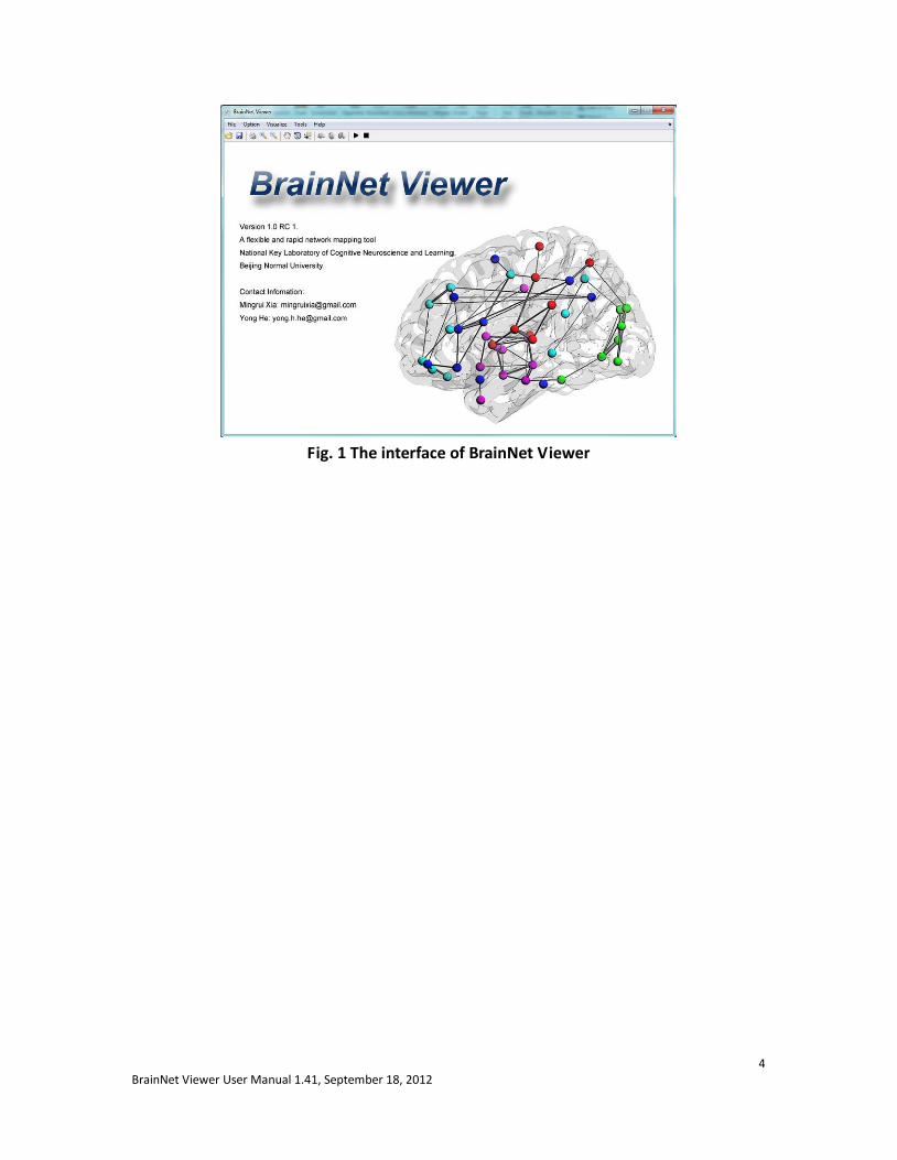
Please contact us if you need standalone version. It cannot be found on the NITRC due to the large size. Install Matlab Components Runtime (MCRInstall.exe for Windows OS, or MCRInstaller.bin for Linux and Mac OS, ~200MB) using default settings. Restart your computer (strongly recommended). Run BrainNet.exe for Windows OS or run_BrainNet.sh for Linux and Mac OS, it should take about one minute to start. You can find the interface below (Fig. 1) after successfully running the BrainNet Viewer.
4 BrainNet Viewer User Manual 1.41, September 18, 2012
Fig. 1 The interface of BrainNet Viewer
5 BrainNet Viewer User Manual 1.41, September 18, 2012
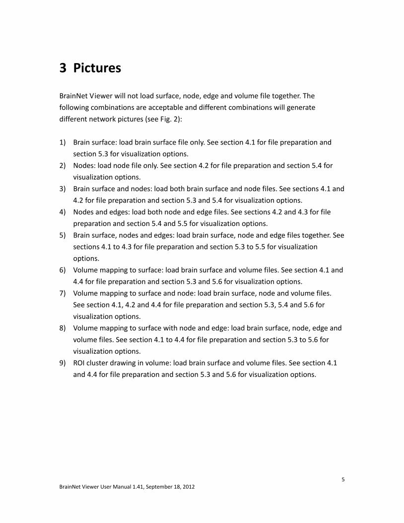
3 Pictures
BrainNet Viewer will not load surface, node, edge and volume file together. The following combinations are acceptable and different combinations will generate different network pictures (see Fig. 2): 1) Brain surface: load brain surface file only. See section 4.1 for file preparation and
section 5.3 for visualization options. 2) Nodes: load node file only. See section 4.2 for file preparation and section 5.4 for
visualization options. 3) Brain surface and nodes: load both brain surface and node files. See sections 4.1 and
4.2 for file preparation and section 5.3 and 5.4 for visualization options. 4) Nodes and edges: load both node and edge files. See sections 4.2 and 4.3 for file
preparation and section 5.4 and 5.5 for visualization options. 5) Brain surface, nodes and edges: load brain surface, node and edge files together. See
sections 4.1 to 4.3 for file preparation and section 5.3 to 5.5 for visualization options.
6) Volume mapping to surface: load brain surface and volume files. See section 4.1 and 4.4 for file preparation and section 5.3 and 5.6 for visualization options.
7) Volume mapping to surface and node: load brain surface, node and volume files. See section 4.1, 4.2 and 4.4 for file preparation and section 5.3, 5.4 and 5.6 for visualization options.
8) Volume mapping to surface with node and edge: load brain surface, node, edge and volume files. See section 4.1 to 4.4 for file preparation and section 5.3 to 5.6 for visualization options.
9) ROI cluster drawing in volume: load brain surface and volume files. See section 4.1 and 4.4 for file preparation and section 5.3 and 5.6 for visualization options.
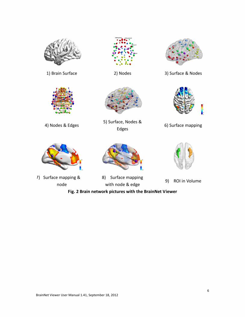
6 BrainNet Viewer User Manual 1.41, September 18, 2012
1) Brain Surface 2) Nodes 3) Surface & Nodes
4) Nodes & Edges 5) Surface, Nodes &
Edges 6) Surface mapping
7) Surface mapping &
node
8) Surface mapping with node & edge
9) ROI in Volume
Fig. 2 Brain network pictures with the BrainNet Viewer
7 BrainNet Viewer User Manual 1.41, September 18, 2012
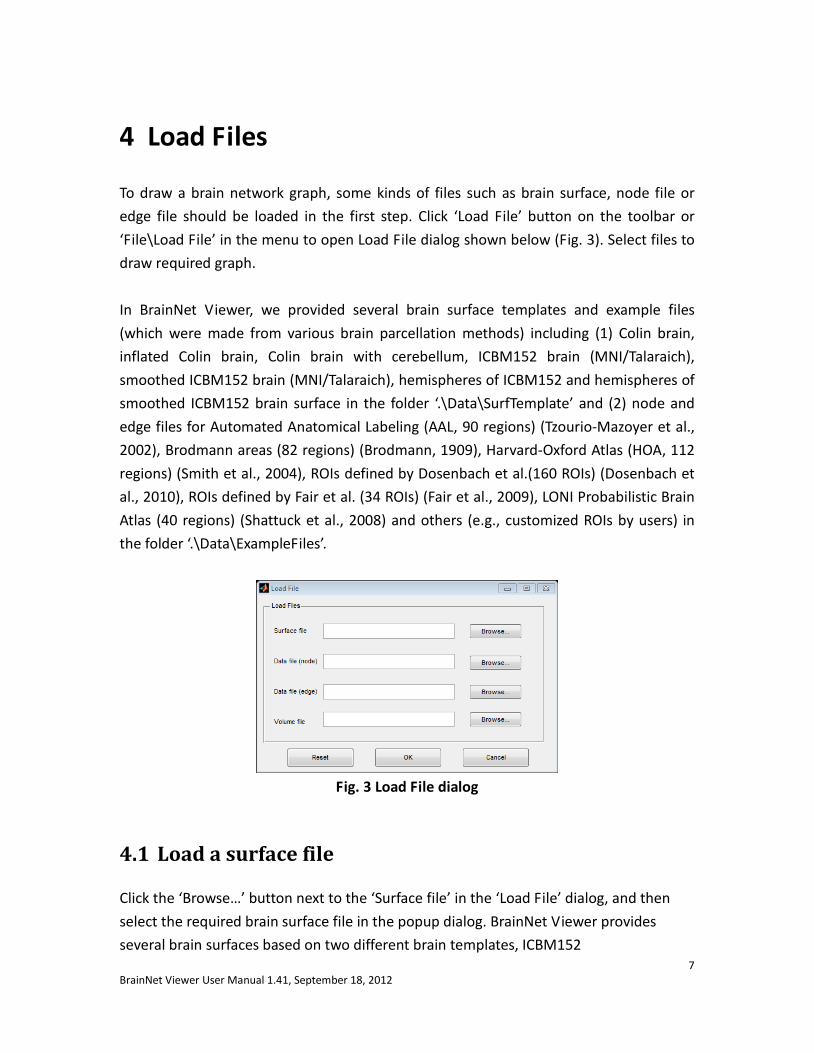
4 Load Files
To draw a brain network graph, some kinds of files such as brain surface, node file or edge file should be loaded in the first step. Click ‘Load File’ button on the toolbar or ‘File\Load File’ in the menu to open Load File dialog shown below (Fig. 3). Select files to draw required graph. In BrainNet Viewer, we provided several brain surface templates and example files (which were made from various brain parcellation methods) including (1) Colin brain, inflated Colin brain, Colin brain with cerebellum, ICBM152 brain (MNI/Talaraich), smoothed ICBM152 brain (MNI/Talaraich), hemispheres of ICBM152 and hemispheres of smoothed ICBM152 brain surface in the folder ‘.\Data\SurfTemplate’ and (2) node and edge files for Automated Anatomical Labeling (AAL, 90 regions) (Tzourio-Mazoyer et al., 2002), Brodmann areas (82 regions) (Brodmann, 1909), Harvard-Oxford Atlas (HOA, 112 regions) (Smith et al., 2004), ROIs defined by Dosenbach et al.(160 ROIs) (Dosenbach et al., 2010), ROIs defined by Fair et al. (34 ROIs) (Fair et al., 2009), LONI Probabilistic Brain Atlas (40 regions) (Shattuck et al., 2008) and others (e.g., customized ROIs by users) in the folder ‘.\Data\ExampleFiles’.
Fig. 3 Load File dialog
4.1 Load a surface file
Click the ‘Browse…’ button next to the ‘Surface file’ in the ‘Load File’ dialog, and then select the required brain surface file in the popup dialog. BrainNet Viewer provides several brain surfaces based on two different brain templates, ICBM152
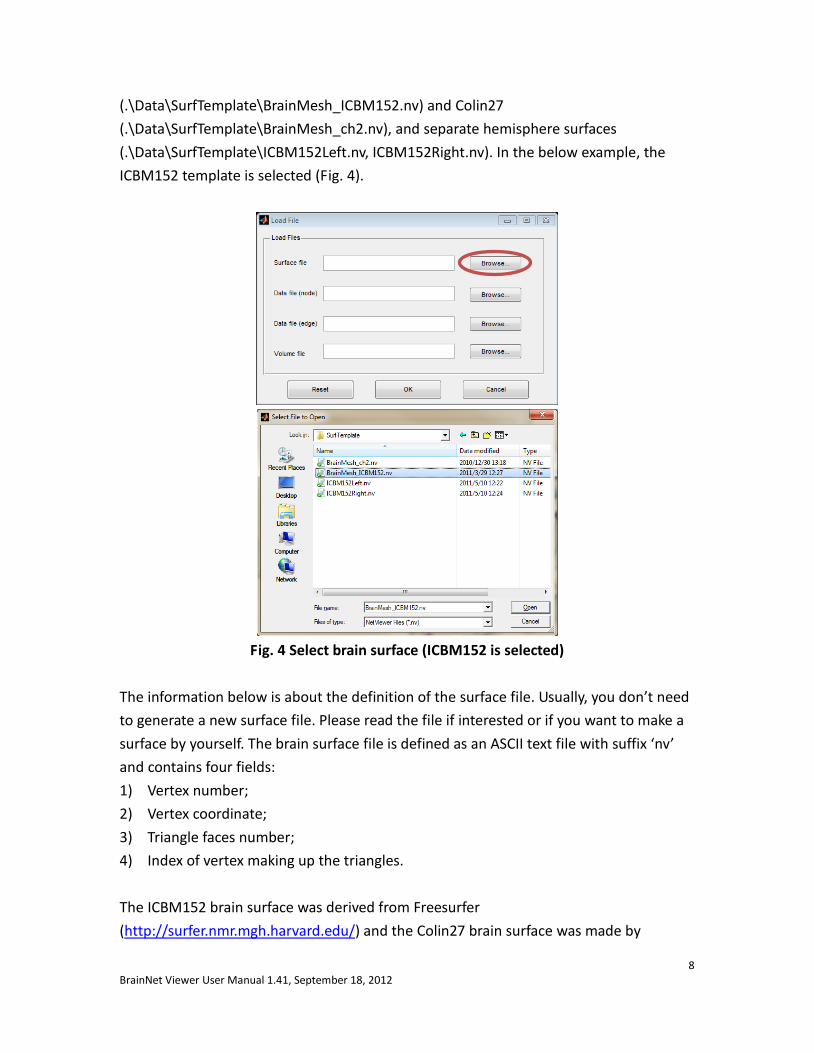
8 BrainNet Viewer User Manual 1.41, September 18, 2012
(.\Data\SurfTemplate\BrainMesh_ICBM152.nv) and Colin27 (.\Data\SurfTemplate\BrainMesh_ch2.nv), and separate hemisphere surfaces (.\Data\SurfTemplate\ICBM152Left.nv, ICBM152Right.nv). In the below example, the ICBM152 template is selected (Fig. 4).
Fig. 4 Select brain surface (ICBM152 is selected)
The information below is about the definition of the surface file. Usually, you don’t need to generate a new surface file. Please read the file if interested or if you want to make a surface by yourself. The brain surface file is defined as an ASCII text file with suffix ‘nv’ and contains four fields: 1) Vertex number; 2) Vertex coordinate; 3) Triangle faces number; 4) Index of vertex making up the triangles. The ICBM152 brain surface was derived from Freesurfer (http://surfer.nmr.mgh.harvard.edu/) and the Colin27 brain surface was made by
9 BrainNet Viewer User Manual 1.41, September 18, 2012
BrainVISA (http://brainvisa.info/). We transferred and merged the original bilateral hemisphere files into one ‘.nv’ file. A surface merge tool is in the tools menu (see more details in section 6.4 ‘Menus\Tool’). Currently, the ‘*.pial’ files generated by FreeSurfer, (only hemisphere mesh) and the ‘*.mesh’ files generated by BrainVISA are supported, and these can be loaded and visualized directly. The FreeSurfer pial files are recommended as their vertex coordinates have been transformed into the MNI space, while the BrainVISA mesh files may need a manual transformation. The ICBM152Left.nv and ICBM152Right.nv files are from Professor Alan Evans’s group in the Montreal Neurological Institute, McGill University. Of note, the coordinates in the surfaces are located in the MNI space.
4.2 Load a node file
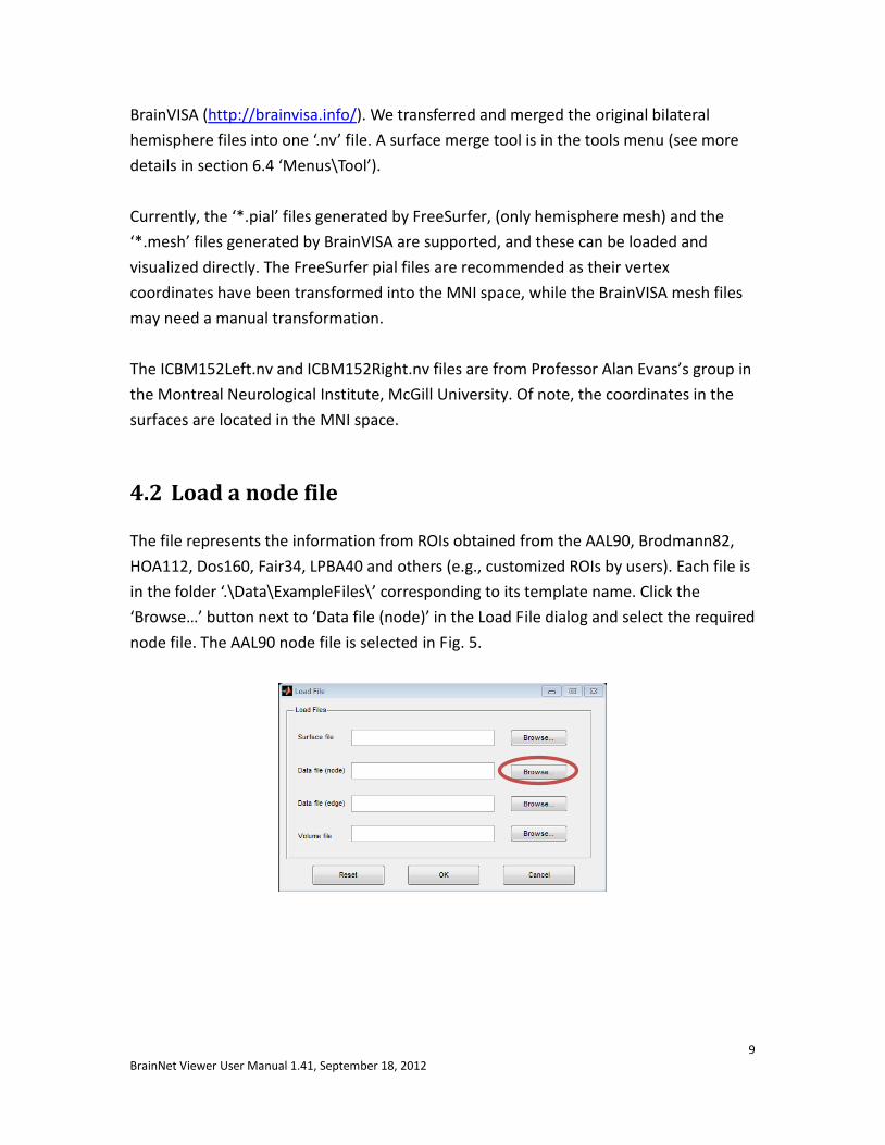
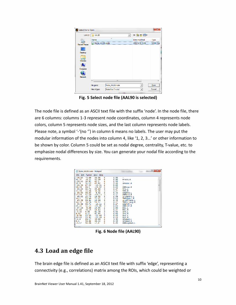
The file represents the information from ROIs obtained from the AAL90, Brodmann82, HOA112, Dos160, Fair34, LPBA40 and others (e.g., customized ROIs by users). Each file is in the folder ‘.\Data\ExampleFiles\’ corresponding to its template name. Click the ‘Browse…’ button next to ‘Data file (node)’ in the Load File dialog and select the required node file. The AAL90 node file is selected in Fig. 5.
10 BrainNet Viewer User Manual 1.41, September 18, 2012
Fig. 5 Select node file (AAL90 is selected)
The node file is defined as an ASCII text file with the suffix ‘node’. In the node file, there are 6 columns: columns 1-3 represent node coordinates, column 4 represents node colors, column 5 represents node sizes, and the last column represents node labels. Please note, a symbol ‘-‘(no ‘’) in column 6 means no labels. The user may put the modular information of the nodes into column 4, like ‘1, 2, 3…’ or other information to be shown by color. Column 5 could be set as nodal degree, centrality, T-value, etc. to emphasize nodal differences by size. You can generate your nodal file according to the requirements.
Fig. 6 Node file (AAL90)
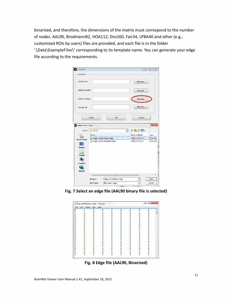
4.3 Load an edge file
The brain edge file is defined as an ASCII text file with suffix ‘edge’, representing a connectivity (e.g., correlations) matrix among the ROIs, which could be weighted or
11 BrainNet Viewer User Manual 1.41, September 18, 2012
binarized, and therefore, the dimensions of the matrix must correspond to the number of nodes. AAL90, Brodmann82, HOA112, Dos160, Fair34, LPBA40 and other (e.g., customized ROIs by users) files are provided, and each file is in the folder ‘.\Data\ExampleFiles\’ corresponding to its template name. You can generate your edge file according to the requirements.
Fig. 7 Select an edge file (AAL90 binary file is selected)
Fig. 8 Edge file (AAL90, Binarized)
12 BrainNet Viewer User Manual 1.41, September 18, 2012
Both node and edge files can be generated/edited with text editors or Excel.
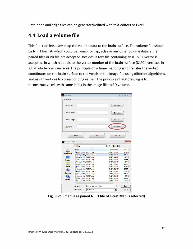
4.4 Load a volume file
This function lets users map the volume data to the brain surface. The volume file should be NIFTI format, which could be T-map, Z-map, atlas or any other volume data, either paired files or nii file are accepted. Besides, a text file containing an n × 1 vector is accepted, in which n equals to the vertex number of the brain surface (81924 vertexes in ICBM whole brain surface). The principle of volume mapping is to transfer the vertex coordinates on the brain surface to the voxels in the image file using different algorithms, and assign vertices to corresponding values. The principle of ROI drawing is to reconstruct voxels with same index in the image file to 3D volume.
Fig. 9 Volume file (a paired NIFTI file of T-test Map is selected)
13 BrainNet Viewer User Manual 1.41, September 18, 2012
5 Visualize option
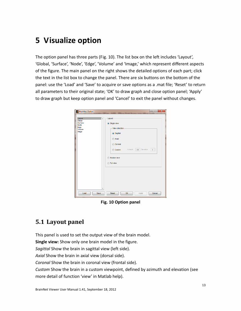
The option panel has three parts (Fig. 10). The list box on the left includes ‘Layout’, ‘Global, ‘Surface’, ‘Node’, ‘Edge’, ’Volume’ and ‘Image,’ which represent different aspects of the figure. The main panel on the right shows the detailed options of each part; click the text in the list box to change the panel. There are six buttons on the bottom of the panel: use the ‘Load’ and ‘Save’ to acquire or save options as a .mat file; ‘Reset’ to return all parameters to their original state; ‘OK’ to draw graph and close option panel; ‘Apply’ to draw graph but keep option panel and ‘Cancel’ to exit the panel without changes.
Fig. 10 Option panel
5.1 Layout panel
This panel is used to set the output view of the brain model. Single view: Show only one brain model in the figure. Sagittal Show the brain in sagittal view (left side). Axial Show the brain in axial view (dorsal side). Coronal Show the brain in coronal view (frontal side). Custom Show the brain in a custom viewpoint, defined by azimuth and elevation (see more detail of function ‘view’ in Matlab help).
14 BrainNet Viewer User Manual 1.41, September 18, 2012
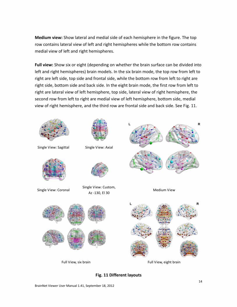
Medium view: Show lateral and medial side of each hemisphere in the figure. The top row contains lateral view of left and right hemispheres while the bottom row contains medial view of left and right hemispheres. Full view: Show six or eight (depending on whether the brain surface can be divided into left and right hemispheres) brain models. In the six brain mode, the top row from left to right are left side, top side and frontal side, while the bottom row from left to right are right side, bottom side and back side. In the eight brain mode, the first row from left to right are lateral view of left hemisphere, top side, lateral view of right hemisphere, the second row from left to right are medial view of left hemisphere, bottom side, medial view of right hemisphere, and the third row are frontal side and back side. See Fig. 11.
Single View: Sagittal Single View: Axial
Single View: Coronal Single View: Custom,
Az -130, El 30 Medium View
Full View, six brain Full View, eight brain
Fig. 11 Different layouts
15 BrainNet Viewer User Manual 1.41, September 18, 2012
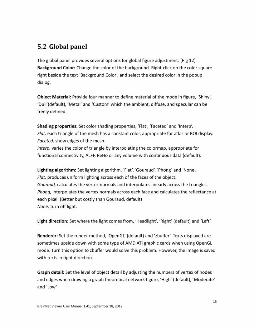
5.2 Global panel
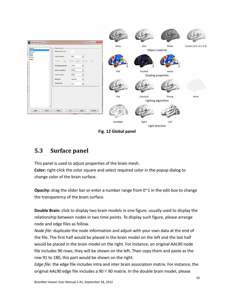
The global panel provides several options for global figure adjustment. (Fig 12) Background Color: Change the color of the background. Right-click on the color square right beside the text ‘Background Color’, and select the desired color in the popup dialog. Object Material: Provide four manner to define material of the mode in figure, ‘Shiny’, ‘Dull’(default), ’Metal’ and ‘Custom’ which the ambient, diffuse, and specular can be freely defined. Shading properties: Set color shading properties, ‘Flat’, ‘Faceted’ and ‘Interp’. Flat, each triangle of the mesh has a constant color, appropriate for atlas or ROI display. Faceted, show edges of the mesh. Interp, varies the color of triangle by interpolating the colormap, appropriate for functional connectivity, ALFF, ReHo or any volume with continuous data (default). Lighting algorithm: Set lighting algorithm, ‘Flat’, ‘Gouraud’, ‘Phong’ and ‘None’. Flat, produces uniform lighting across each of the faces of the object. Gouraud, calculates the vertex normals and interpolates linearly across the triangles. Phong, interpolates the vertex normals across each face and calculates the reflectance at each pixel. (Better but costly than Gouraud, default) None, turn off light. Light direction: Set where the light comes from, ‘Headlight’, ‘Right’ (default) and ‘Left’. Renderer: Set the render method, ‘OpenGL’ (default) and ‘zbuffer’. Texts displayed are sometimes upside down with some type of AMD ATI graphic cards when using OpenGL mode. Turn this option to zbuffer would solve this problem. However, the image is saved with texts in right direction. Graph detail: Set the level of object detail by adjusting the numbers of vertex of nodes and edges when drawing a graph theoretical network figure, ‘High’ (default), ’Moderate’ and ‘Low’
16 BrainNet Viewer User Manual 1.41, September 18, 2012
Shiny Dull Metal Custom (0.5, 0.5, 0.5)
Object material
Flat Faceted Interp
Shading properties
Flat Gouraud Phong None
Lighting algorithim
Headlight Right Left
Light direction
Fig. 12 Global panel
5.3 Surface panel
This panel is used to adjust properties of the brain mesh. Color: right-click the color square and select required color in the popup dialog to change color of the brain surface. Opacity: drag the slider bar or enter a number range from 0~1 in the edit box to change the transparency of the brain surface. Double Brain: click to display two brain models in one figure, usually used to display the relationship between nodes in two time points. To display such figure, please arrange node and edge files as follow. Node file: duplicate the node information and adjust with your own data at the end of the file. The first half would be placed in the brain model on the left and the last half would be placed in the brain model on the right. For instance, an original AAL90 node file includes 90 rows; they will be shown on the left. Then copy them and paste as the row 91 to 180, this part would be shown on the right. Edge file: the edge file includes intra and inter brain association matrix. For instance, the original AAL90 edge file includes a 90×90 matrix. In the double brain model, please
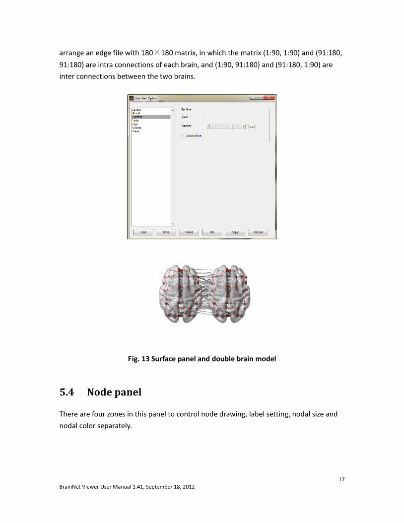
17 BrainNet Viewer User Manual 1.41, September 18, 2012
arrange an edge file with 180×180 matrix, in which the matrix (1:90, 1:90) and (91:180, 91:180) are intra connections of each brain, and (1:90, 91:180) and (91:180, 1:90) are inter connections between the two brains.
Fig. 13 Surface panel and double brain model
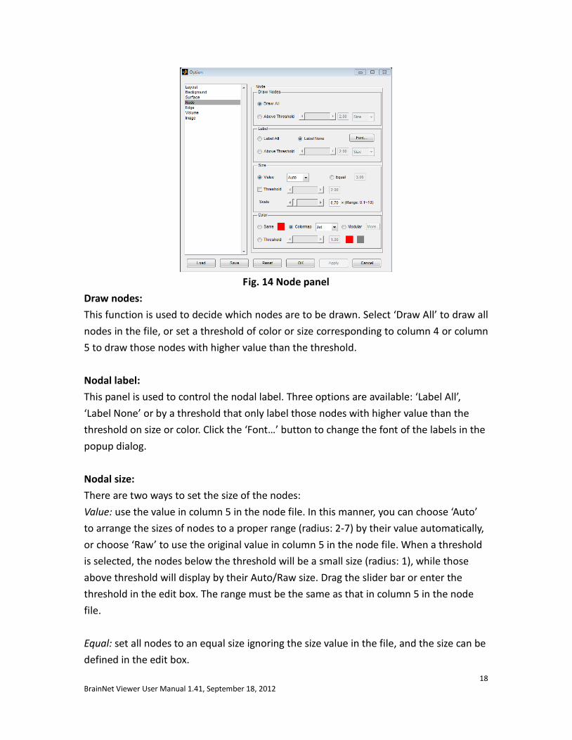
5.4 Node panel
There are four zones in this panel to control node drawing, label setting, nodal size and nodal color separately.
18 BrainNet Viewer User Manual 1.41, September 18, 2012
Fig. 14 Node panel
Draw nodes: This function is used to decide which nodes are to be drawn. Select ‘Draw All’ to draw all nodes in the file, or set a threshold of color or size corresponding to column 4 or column 5 to draw those nodes with higher value than the threshold. Nodal label: This panel is used to control the nodal label. Three options are available: ‘Label All’, ‘Label None’ or by a threshold that only label those nodes with higher value than the threshold on size or color. Click the ‘Font…’ button to change the font of the labels in the popup dialog. Nodal size: There are two ways to set the size of the nodes: Value: use the value in column 5 in the node file. In this manner, you can choose ‘Auto’ to arrange the sizes of nodes to a proper range (radius: 2-7) by their value automatically, or choose ‘Raw’ to use the original value in column 5 in the node file. When a threshold is selected, the nodes below the threshold will be a small size (radius: 1), while those above threshold will display by their Auto/Raw size. Drag the slider bar or enter the threshold in the edit box. The range must be the same as that in column 5 in the node file. Equal: set all nodes to an equal size ignoring the size value in the file, and the size can be defined in the edit box.
19 BrainNet Viewer User Manual 1.41, September 18, 2012
Scale: the volume ratio option is used to adjust the size of all nodes together, and the scale factor ranges from 0.1 to 10. Nodal color: This panel provides four ways to control nodal color: Same: to use the same color for all nodes ignoring the color index in the file, right-click the color square and select the required color from the popup dialog. Colormap: use a color map to display the value of the nodes from low end to high end corresponding to column 4 in the node file. 13 kinds of color maps can be selected (see the right picture for detail).
Modular: modular color can be used to display different nodal colors for different modules. Set the values of column 4 as ‘1, 2, 3…’ corresponding to modular 1, modular 2… in the node file. The maximum number of modules is21 at present. Click to open the modular color dialog, and the left picture will display six modules with their color on the right. Click the popup menus on the left to select other modules in the list and the color square will change to
the corresponding one. Right-click the color square to change color as described above. Threshold: to binarize the color by a given threshold, drag the slider bar or enter the threshold in the edit box, but the range must be the same as the range stated in column 4 of the node file. The nodes with higher value will have one fixed color, while the nodes with lower value will have another fixed color. Right-click the color square to select the color – the left one represents the higher value color while the right one represents the lower value color.
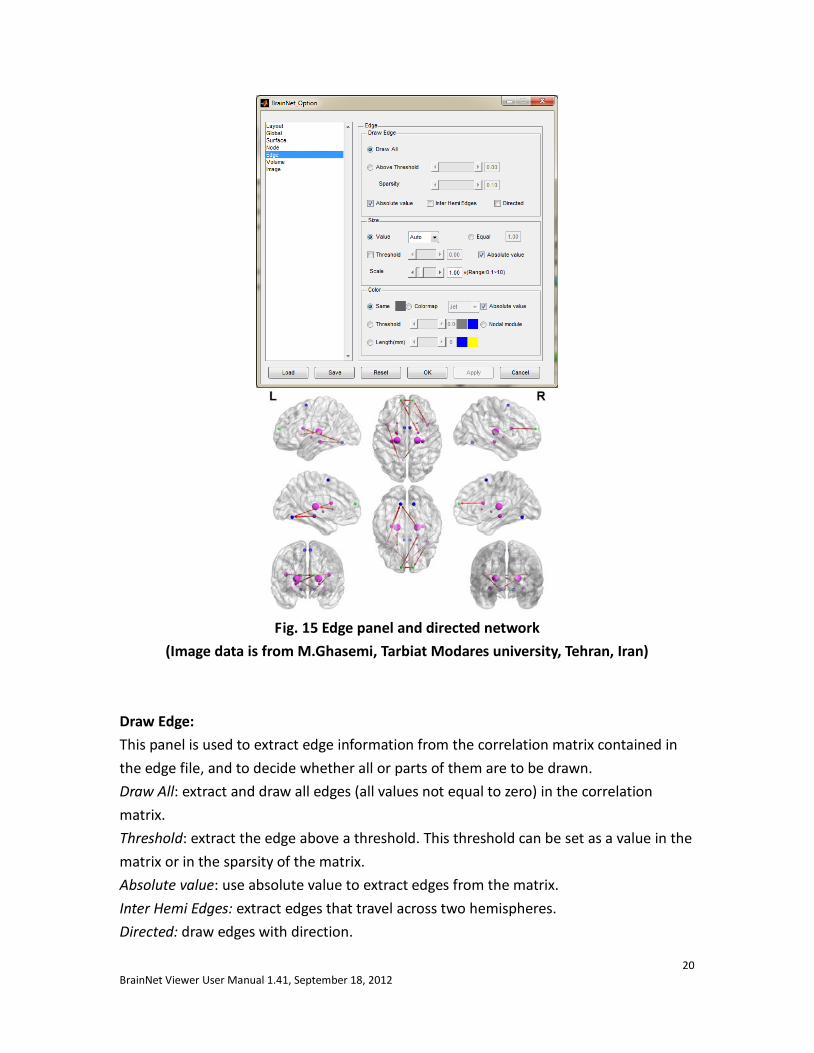
5.5 Edge panel
There are three parts in this panel to control edge drawing, edge size and edge color separately.
20 BrainNet Viewer User Manual 1.41, September 18, 2012
Fig. 15 Edge panel and directed network
(Image data is from M.Ghasemi, Tarbiat Modares university, Tehran, Iran) Draw Edge: This panel is used to extract edge information from the correlation matrix contained in the edge file, and to decide whether all or parts of them are to be drawn. Draw All: extract and draw all edges (all values not equal to zero) in the correlation matrix. Threshold: extract the edge above a threshold. This threshold can be set as a value in the matrix or in the sparsity of the matrix. Absolute value: use absolute value to extract edges from the matrix. Inter Hemi Edges: extract edges that travel across two hemispheres. Directed: draw edges with direction.

21 BrainNet Viewer User Manual 1.41, September 18, 2012
Note that BrainNet Viewer will treat the value zero (0) in the matrix as a null edge, and only the right upper triangle of the matrix will be considered in undirected mode. Always remember to change the threshold when a weighted matrix is loaded, or it will draw the full connection among the nodes, which would require a lot of time. Edge size: There are two ways to set the size of edges (here, size means the radius of the edge); Value: employ the correlation matrix value in the edge file. In this manner, you can choose ‘Auto’ to assign the edge sizes a proper range (radius: 0.3-1.5) by their value automatically or choose ‘Raw’ to use the original value of the correlation matrix in the edge file. When a threshold is selected, the edges with values lower than the threshold will have a fixed, smaller size while the edges above threshold will be shown as Auto/Raw size. Drag the slider bar or enter the threshold into the edit box, but the range must be the same as the correlation matrix in the edge file. Equal: set all edges to an equal size, and the size can be defined in the edit box. Scale: the scale option is used to adjust the size of all edges together. The scale factor ranges from 0.1 to 10. Absolute value: use absolute value in matrix to calculate edge radius. Edge color: This panel provides five ways to control edge color: Same: adopt the same color for all edges, right-click the color square and select the required color from the popup dialog. Colormap: use a colormap to render the value of the edge from low to high corresponding to the values of the correlation matrix in the edge file. 13 kinds of colormaps, same as the nodal colormaps can be selected. Threshold: binarize the color by a given threshold, drag the slider bar or enter the threshold into the edit box. The range must be the same as the correlation matrix in the edge file. Right-click the color square to select colors – the left one represents the lower value while the right one represents the higher value.
22 BrainNet Viewer User Manual 1.41, September 18, 2012
Length: binarize the color by a given threshold of Euclidean distance between two nodes (mm). The edges with longer length have one fixed color, while the shorter ones have another fixed color. Drag the slider bar or enter the threshold in the edit box; the threshold can range from zero to 100. Right-click the color square to select colors, the left one represents the higher value while the right one represents the lower value. Nodal module: assign edge color according to the color of nodes it links. If two nodes of the edge have same color, the edge will be set as the same color. If the two nodes are with different color, the edge will be colored gray. Absolute value: use absolute value in matrix to calculate edge color.
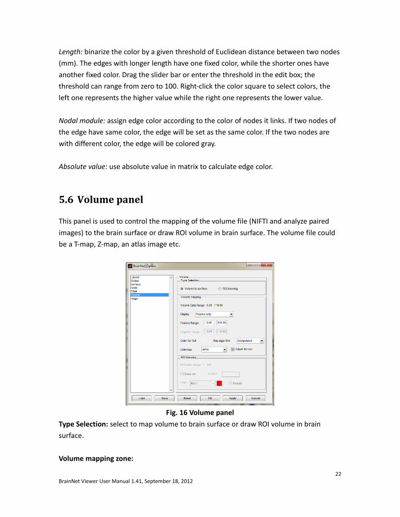
5.6 Volume panel
This panel is used to control the mapping of the volume file (NIFTI and analyze paired images) to the brain surface or draw ROI volume in brain surface. The volume file could be a T-map, Z-map, an atlas image etc.
Fig. 16 Volume panel
Type Selection: select to map volume to brain surface or draw ROI volume in brain surface. Volume mapping zone:

23 BrainNet Viewer User Manual 1.41, September 18, 2012
Volume Data Range: show the minimum and maximum values of the volume file. Display: contain three mapping manner, ‘Positive & Negative’, ‘Positive only’ and ‘Negative only’. ‘Positive & Negative’ sets the colorbar range from the minimum negative value to the maximum positive value, and ‘Positive only’ and ‘Negative only’ just set the range of the colorbar in positive value or negative value separately. Positive Range and Negative Range: set the range of the color bar. The edit boxes on the left define the value near zero on the color bar, while the right ones define the value away from zero. Take the above picture as an example. When ‘Positive & Negative’ is chosen, the color bar would be arranged from -3 to 3, and -0.01 to 0.01 would be set as the null value range; if ‘Positive only’ is selected, the color bar would be arranged from 0.01 to 3, any value below 0.01 would be set as a null value; and if ‘Negative only’ is selected, the color bar would be arranged from -0.01 to -3, and any value above -0.01 would be set as a null value (see Fig. 17). Color for Null: define the color for null value part on the surface. Right-click the color square and select required color. Adjust for Null: when this option is selected, the colormap will be adjusted for null value vertex. Specifically, in Positive & Negative mode, the vertex with value between high end of negative interval and low end of positive interval will be set as color for null; in only positive mode, the vertex with value below the low end of positive interval will be set as color for null; and in only negative mode, the vertex with value larger than the low end of positive interval will be set as color for null. Colormap: provide 24 kinds of colormaps including custom colormap. Map algorithm: eight mapping algorithms are provided. ‘Nearest Voxel’, assign the vertex with the value of voxel in volume that is nearest to it, suitable for atlas and mask; ‘Average Vertex’, assign the vertex with the value of voxel in volume that is nearest to it, then average the vertex across its neighbors (time costly); ‘Average Voxel’, assign the vertex with the average value of voxel and its neighbors in volume that is nearest to it; ‘Gaussian’, the volume is first smoothed by a Gaussian kernel, and then assign the vertex with the value of voxel in volume that is nearest to it; ‘Interpolated’ (default), the coordinate of the vertex is determined in the volume, trilinear interpolate method is then used across its neighbors to calculate the value; ‘Maximum Voxel’, assign the vertex
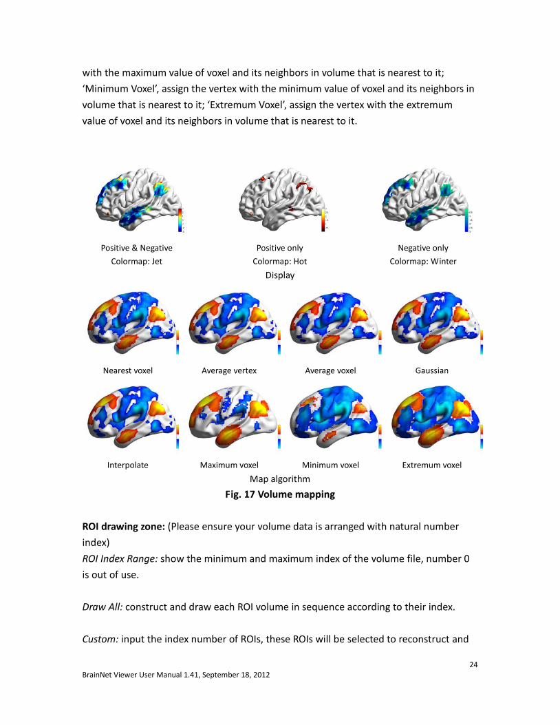
24 BrainNet Viewer User Manual 1.41, September 18, 2012
with the maximum value of voxel and its neighbors in volume that is nearest to it; ‘Minimum Voxel’, assign the vertex with the minimum value of voxel and its neighbors in volume that is nearest to it; ‘Extremum Voxel’, assign the vertex with the extremum value of voxel and its neighbors in volume that is nearest to it.
Positive & Negative
Colormap: Jet Positive only
Colormap: Hot Negative only
Colormap: Winter Display
Nearest voxel Average vertex Average voxel Gaussian
Interpolate Maximum voxel Minimum voxel Extremum voxel
Map algorithm Fig. 17 Volume mapping
ROI drawing zone: (Please ensure your volume data is arranged with natural number index) ROI Index Range: show the minimum and maximum index of the volume file, number 0 is out of use. Draw All: construct and draw each ROI volume in sequence according to their index. Custom: input the index number of ROIs, these ROIs will be selected to reconstruct and
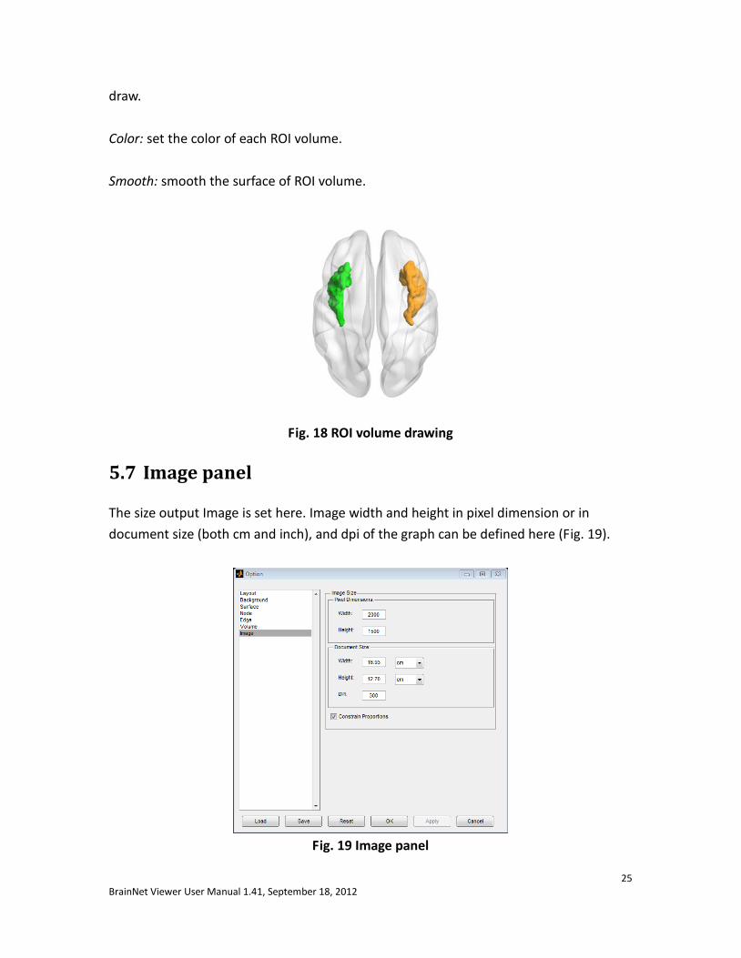
25 BrainNet Viewer User Manual 1.41, September 18, 2012
draw. Color: set the color of each ROI volume. Smooth: smooth the surface of ROI volume.
Fig. 18 ROI volume drawing
5.7 Image panel
The size output Image is set here. Image width and height in pixel dimension or in document size (both cm and inch), and dpi of the graph can be defined here (Fig. 19).
Fig. 19 Image panel
26 BrainNet Viewer User Manual 1.41, September 18, 2012
6 Menu
6.1 Files
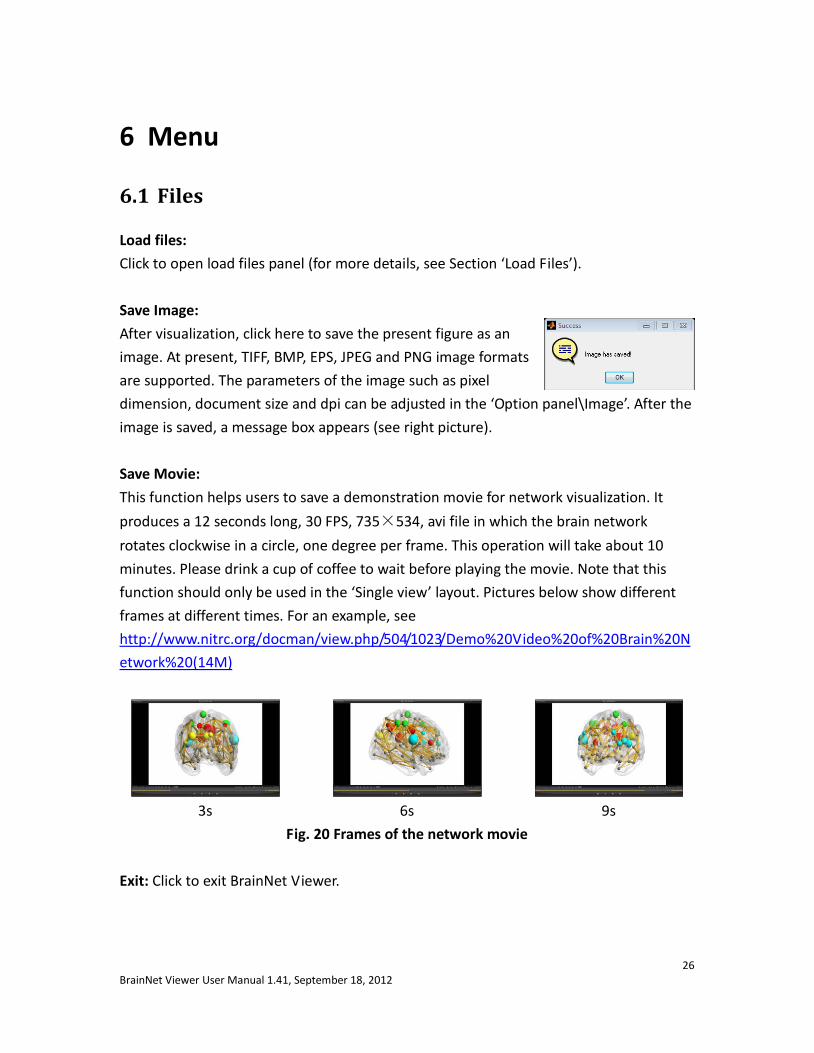
Load files: Click to open load files panel (for more details, see Section ‘Load Files’). Save Image: After visualization, click here to save the present figure as an image. At present, TIFF, BMP, EPS, JPEG and PNG image formats are supported. The parameters of the image such as pixel dimension, document size and dpi can be adjusted in the ‘Option panel\Image’. After the image is saved, a message box appears (see right picture). Save Movie: This function helps users to save a demonstration movie for network visualization. It produces a 12 seconds long, 30 FPS, 735×534, avi file in which the brain network rotates clockwise in a circle, one degree per frame. This operation will take about 10 minutes. Please drink a cup of coffee to wait before playing the movie. Note that this function should only be used in the ‘Single view’ layout. Pictures below show different frames at different times. For an example, see http://www.nitrc.org/docman/view.php/504/1023/Demo%20Video%20of%20Brain%20Network%20(14M)
3s 6s 9s
Fig. 20 Frames of the network movie Exit: Click to exit BrainNet Viewer.
27 BrainNet Viewer User Manual 1.41, September 18, 2012
6.2 Option
Option: Click to open the option panel (see more details in section ‘Visualize Option’). Load Option: Load a previously saved visualize option file. Save Option: Save current visualize option as a *.mat file. Colormap Editor: Call colomap editor to edit colormap manually. Apply Colormap: Apply edited colormap by colormap editor to all graphs in figure. Save Colormap: save colormap as a text file. The saved colormap can be used by copy its text into custom colormap in option panel.
6.3 Visualize
Redraw: Clear figure and redraw network using the data and option last loaded. Clear Figure: Remove brain network and display the default information of BrainNet Viewer.
6.4 Tools
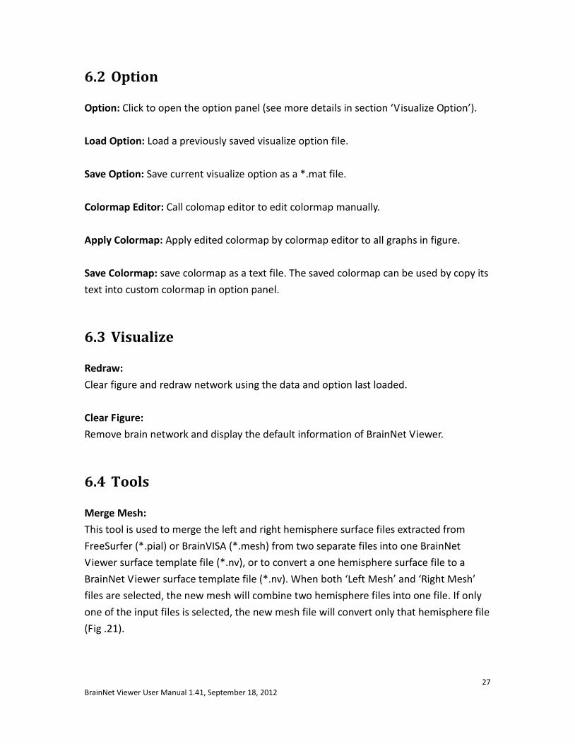
Merge Mesh: This tool is used to merge the left and right hemisphere surface files extracted from FreeSurfer (*.pial) or BrainVISA (*.mesh) from two separate files into one BrainNet Viewer surface template file (*.nv), or to convert a one hemisphere surface file to a BrainNet Viewer surface template file (*.nv). When both ‘Left Mesh’ and ‘Right Mesh’ files are selected, the new mesh will combine two hemisphere files into one file. If only one of the input files is selected, the new mesh file will convert only that hemisphere file (Fig .21).
28 BrainNet Viewer User Manual 1.41, September 18, 2012
Fig. 21 Merge Meshes tool
6.5 Help
Manual: Open this manual for help. About: Show version, author and contact information of BrainNet Viewer in a dialog.
29 BrainNet Viewer User Manual 1.41, September 18, 2012
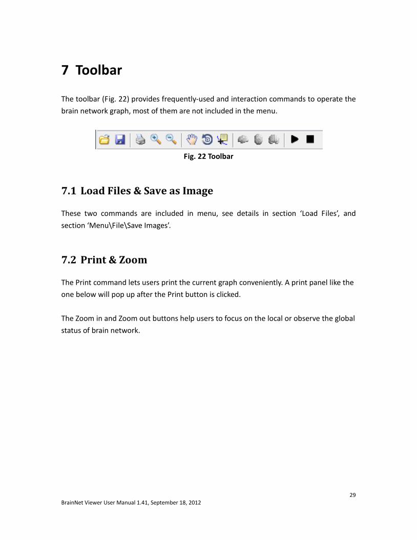
7 Toolbar
The toolbar (Fig. 22) provides frequently-used and interaction commands to operate the brain network graph, most of them are not included in the menu.
Fig. 22 Toolbar
7.1 Load Files & Save as Image
These two commands are included in menu, see details in section ‘Load Files’, and section ‘Menu\File\Save Images’.
7.2 Print & Zoom
The Print command lets users print the current graph conveniently. A print panel like the one below will pop up after the Print button is clicked. The Zoom in and Zoom out buttons help users to focus on the local or observe the global status of brain network.

30 BrainNet Viewer User Manual 1.41, September 18, 2012
Print panel Zoom in & Zoom out
Fig. 23 Print panel and Zoom function
7.3 Move, Rotate & Get position
Click the ‘Move’ button and drag the brain anywhere in the window. When the ‘Rotate’ button is pressed, hold left button of the mouse and move mouse to rotate the brain. When rotate button is deselected, the light cam in the window will re-render the brain model depending on the current orientation. Click the ‘Get position’ button, and then click on the surface of the brain to show the coordinate of the vertex. Right click anywhere in the figure window, and select ‘Delete All Datatips’ to remove all coordinate labels.
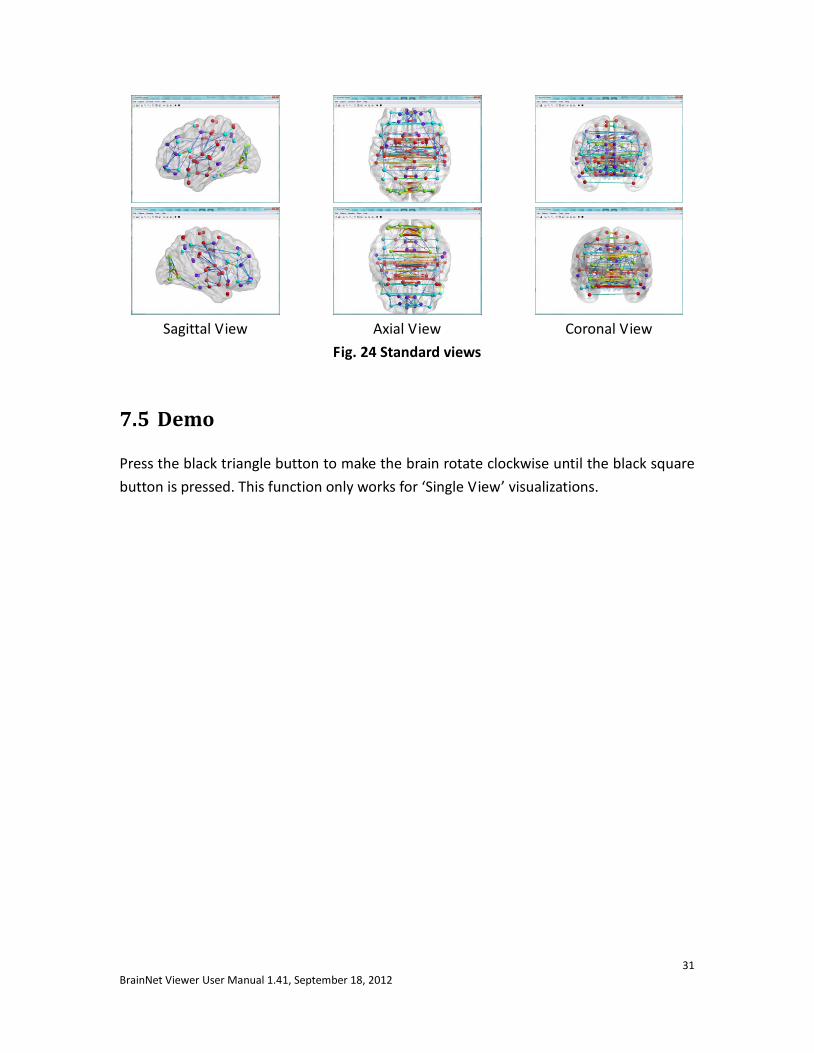
7.4 Standard view
Three standard views, sagittal, axial and coronal view buttons are available to help users observe networks from different standard views quickly. These buttons should only be used for ‘Single view’ visualized brain networks. Click twice to see the opposite side of the brain.
31 BrainNet Viewer User Manual 1.41, September 18, 2012
Sagittal View Axial View Coronal View
Fig. 24 Standard views
7.5 Demo
Press the black triangle button to make the brain rotate clockwise until the black square button is pressed. This function only works for ‘Single View’ visualizations.

32 BrainNet Viewer User Manual 1.41, September 18, 2012
Acknowledgements
We thank the following colleagues for their kind helps during BrainNet Viewer developing and manual revising: Dr. G. Gong, Dr. N. Shu, Dr. C. Yan, Mr. J. Wang, Mr. T. Xie, Mr. Q. Lin, Ms. Z. Dai, Ms. M. Cao and Ms. J. Zhang, National Key Laboratory of Cognitive Neuroscience and Learning, Beijing Normal University, China; Professor A. Evans, McGill University, Canada; Mr. P. Clark, Pennsylvania State University, USA; Mr. M.Ghasemi, Tarbiat Modares University, Iran. We also thank the developers of the following softwares and toolboxes whose source codes or file formats were referenced during our package developing: Matlab: www.mathworks.com/products/matlab/ SurfStat: www.math.mcgill.ca/keith/surfstat/ FreeSurfer: http://surfer.nmr.mgh.harvard.edu/ BrainVISA: http://brainvisa.info/ SPM: www.fil.ion.ucl.ac.uk/spm/ This work was supported by the Natural Science Foundation of China (Grant Nos. 81030028 and 30870667) and Beijing Natural Science Foundation (Grant No. 7102090).
33 BrainNet Viewer User Manual 1.41, September 18, 2012
Reference
Brodmann K (1909) Vergleichende lokalisationslehre der grobhirnrinde. Barth: Leipzig.
Dosenbach NU, Nardos B, Cohen AL, Fair DA, Power JD, Church JA, Nelson SM, Wig GS, Vogel AC, Lessov-Schlaggar CN, Barnes KA, Dubis JW, Feczko E, Coalson RS, Pruett JR, Jr., Barch DM, Petersen SE, Schlaggar BL (2010) Prediction of individual brain maturity using fMRI. Science 329:1358-1361.
Fair DA, Cohen AL, Power JD, Dosenbach NU, Church JA, Miezin FM, Schlaggar BL, Petersen SE (2009) Functional brain networks develop from a "local to distributed" organization. PLoS Comput Biol 5:e1000381.
Shattuck DW, Mirza M, Adisetiyo V, Hojatkashani C, Salamon G, Narr KL, Poldrack RA, Bilder RM, Toga AW (2008) Construction of a 3D probabilistic atlas of human cortical structures. Neuroimage 39:1064-1080.
Smith SM, Jenkinson M, Woolrich MW, Beckmann CF, Behrens TE, Johansen-Berg H, Bannister PR, De Luca M, Drobnjak I, Flitney DE, Niazy RK, Saunders J, Vickers J, Zhang Y, De Stefano N, Brady JM, Matthews PM (2004) Advances in functional and structural MR image analysis and implementation as FSL. Neuroimage 23 Suppl 1:S208-219.
Tzourio-Mazoyer N, Landeau B, Papathanassiou D, Crivello F, Etard O, Delcroix N, Mazoyer B, Joliot M (2002) Automated anatomical labeling of activations in SPM using a macroscopic anatomical parcellation of the MNI MRI single-subject brain. Neuroimage 15:273-289.


