OPEN ACCESS Musical genres: beating to the rhythms of different drums To cite this article: Debora C Correa et al 2010 New J. Phys. 12 053030 View the article online for updates and enhancements. You may also like Musical Instrument Recognition using Mel- Frequency Cepstral Coefficients and Learning Vector Quantization I Maliki and Sofiyanudin - Aceh Serune Kale and Rapai Ethnic Musical Instrument Preservation Method Based on Two-Dimensional Multimedia Animation Zulfan and Baihaqi - Semiclassical analysis of Bose–Hubbard dynamics Hagar Veksler and Shmuel Fishman - Recent citations Evolution of Entropy in Art Painting Based on the Wavelet Transform Hongyi Yang and Han Yang - Beauty in artistic expressions through the eyes of networks and physics Matjaž and Perc - Lucas C. Ribas et al - This content was downloaded from IP address 180.246.17.220 on 04/01/2022 at 11:04
Transcript
OPEN ACCESS
Musical genres: beating to the rhythms of differentdrumsTo cite this article: Debora C Correa et al 2010 New J. Phys. 12 053030
View the article online for updates and enhancements.
You may also likeMusical Instrument Recognition using Mel-Frequency Cepstral Coefficients andLearning Vector QuantizationI Maliki and Sofiyanudin
-
Aceh Serune Kale and Rapai EthnicMusical Instrument Preservation MethodBased on Two-Dimensional MultimediaAnimationZulfan and Baihaqi
-
Semiclassical analysis of Bose–HubbarddynamicsHagar Veksler and Shmuel Fishman
-
Recent citationsEvolution of Entropy in Art Painting Basedon the Wavelet TransformHongyi Yang and Han Yang
-
Beauty in artistic expressions through theeyes of networks and physicsMatjaž and Perc
-
Lucas C. Ribas et al-
This content was downloaded from IP address 180.246.17.220 on 04/01/2022 at 11:04
T h e o p e n – a c c e s s j o u r n a l f o r p h y s i c s
New Journal of Physics
Musical genres: beating to the rhythms ofdifferent drums
Debora C Correa1,4, Jose H Saito2 and Luciano da F Costa1,3,4
1 Instituto de Fisica de Sao Carlos - Universidade de Sao Paulo,Av. Trabalhador Sao Carlense 400, Caixa Postal 369, CEP 13560-970,Sao Carlos, Sao Paulo, Brazil2 Departamento de Computacao—Universidade Federal de Sao Carlos,Rodovia Washington Luis, km 235, SP-310, CEP 13565-905, Sao Carlos,Sao Paulo, Brazil3 National Institute of Science and Technology for Complex Systems,24210-346 Niterói, RJ, BrazilE-mail: [email protected] and luciano.if.sc.usp.br
New Journal of Physics 12 (2010) 053030 (37pp)Received 4 December 2009Published 20 May 2010Online at http://www.njp.org/doi:10.1088/1367-2630/12/5/053030
Abstract. Online music databases have increased significantly as a conse-quence of the rapid growth of the Internet and digital audio, requiring the de-velopment of faster and more efficient tools for music content analysis. Musicalgenres are widely used to organize music collections. In this paper, the problemof automatic single and multi-label music genre classification is addressed by ex-ploring rhythm-based features obtained from a respective complex network rep-resentation. A Markov model is built in order to analyse the temporal sequenceof rhythmic notation events. Feature analysis is performed by using two multi-variate statistical approaches: principal components analysis (unsupervised) andlinear discriminant analysis (supervised). Similarly, two classifiers are applied inorder to identify the category of rhythms: parametric Bayesian classifier underthe Gaussian hypothesis (supervised) and agglomerative hierarchical clustering(unsupervised). Qualitative results obtained by using the kappa coefficient andthe obtained clusters corroborated the effectiveness of the proposed method.
4 Authors to whom any correspondence should be addressed.
4. Concluding remarks 25Acknowledgments 31Appendix A. Multivariate statistical methods 31Appendix B. Linear and quadratic discriminant functions 32Appendix C. Agglomerative hierarchical clustering 33Appendix D. The kappa coefficient 34References 35
1. Introduction
Musical databases have increased in number and size continuously, paving the way to largeamounts of online music data, including discographies, biographies and lyrics. This happenedmainly as a consequence of musical publishing being absorbed by the Internet, as well asthe restoration of existing analogue archives and the advancements of web technologies. Asa consequence, more and more reliable and faster tools for music content analysis, retrievaland description are required, catering for browsing, interactive access and music content-basedqueries. Even more promising, these tools, together with the respective online music databases,have opened new perspectives for basic investigations in the field of music.
Within this context, music genres provide particularly meaningful descriptors given thatthey have been extensively used for years to organize music collections. When a musical piecebecomes associated with a genre, users can retrieve what they are searching in a much fastermanner. It is interesting to note that these new possibilities of research in music can complementwhat is known about the trajectories of music genres, their history and their dynamics [1]. In anethnographic manner, music genres are particularly important because they express the generalidentity of the cultural foundations in which they are incorporated [2]. Music genres are partof a complex interplay of cultures, artists and market strategies to define associations betweenmusicians and their works, making the organization of music collections easier [3]. Therefore,musical genres are of great interest because they can summarize some shared characteristicsin music pieces. As indicated in [4], music genre is probably the most common description ofmusic content, and its classification represents an appealing topic in music information retrieval(MIR) research.
New Journal of Physics 12 (2010) 053030 (http://www.njp.org/)
Despite their ample use, music genres are not a clearly defined concept, and theirboundaries remain fuzzy [3]. As a consequence, the development of such a taxonomy iscontroversial and redundant, representing a challenging problem. Pachet and Cazaly [5]demonstrated that there is no general agreement on musical genre taxonomies, which candepend on cultural references. Even widely used terms such as rock, jazz, blues and pop arenot clear and firmly defined. According to Scaringella et al [3], it is necessary to keep inmind what kind of music item is being analysed in genre classification: a song, an album or anartist. While the most natural choice would be a song, it is sometimes questionable to classifyone song into only one genre. Depending on the characteristics, a song can be classified intovarious genres. This happens more intensively with albums and artists, since, nowadays, albumscontain heterogeneous material and the majority of artists tend to cover an ample range ofgenres during their careers. Therefore, it is difficult to associate an album or an artist with aspecific genre. Pachet and Cazaly [5] also mention that the semantic confusion existing in thetaxonomies can cause redundancies that probably will not be confused by human users, but mayhardly be dealt with by automatic systems, so that automatic analysis of the musical databasesbecomes essential. However, all these critical issues emphasize that the problem of automaticclassification of musical genres is a nontrivial task. As a result, only local conclusions aboutgenre taxonomy are considered [5].
Like other problems involving pattern recognition, the process of automatic classificationof musical genres can usually be divided into the following three main steps: representation,feature extraction and the classifier design [6, 7]. Music information can be described bysymbolic representation or based on acoustic signals [8]. The former is a high-level kind ofrepresentation through music scores, such as MIDI, where each note is described in terms ofpitch, duration, start and end times, and strength. Acoustic signals representation is obtainedby sampling the sound waveform. Once the audio signals are represented in the computer, theobjective becomes to extract relevant features in order to improve the classification accuracy.In the case of music, features may belong to its main dimensions including melody, timbre,rhythm and harmony.
After extracting significant features, any classification scheme may be used. There aremany previous works concerning automatic genre classification in the literature [8]–[19].
An innovative approach to automatic genre classification is proposed in the current work, inwhich musical features refer to the temporal aspects of the songs: the rhythm. Thus, we proposeto identify the genres in terms of their rhythmic patterns. While there is no clear definition ofrhythm [3], it is possible to relate it to the idea of temporal regularity. More generally speaking,rhythm can be simply understood as a specific pattern produced by notes differing in duration,pause and stress. Hence, it is simpler to obtain and manipulate rhythm than the whole melodiccontent. However, despite its simplicity, the rhythm is genuine and intuitively characteristicand intrinsic to musical genres, since, for example, it can be used to distinguish between rockmusic and rhythmically more complex music, such as salsa. In addition, the rhythm is largelyindependent of the instrumentation and interpretation.
A few related works that use rhythm as features in automatic genre recognition can befound in the literature. The work of Akhtaruzzaman [20], in which rhythm is analysed in termsof mathematical and geometrical properties, and then fed to a system for the classificationof rhythms from different regions. Karydis [21] proposed to classify intra-classical genreswith note pitch and duration features, obtained from their histograms. Reviews of existingautomatic rhythm description systems are presented in [22, 23]. The authors state that despite
New Journal of Physics 12 (2010) 053030 (http://www.njp.org/)
the consensus on some rhythm concepts, there is not a single representation of rhythm thatwould be applicable for different applications, such as tempo and meter induction, beat tracking,quantization of rhythm and so on. They also analysed the relevance of these descriptors bymeasuring their performance in genre classification experiments. It has been observed thatmany of these approaches lack comprehensiveness because of the relatively limited rhythmrepresentations that have been adopted [3].
Nowadays, multi-label classification methods are increasingly required by applicationssuch as text categorization [24], scene classification [25], protein classification [26] andmusic categorization in terms of emotion [27], among others. The possibility of multigenresclassification is particularly promising and probably closer to the human experience.
In the current study, an objective and systematic analysis of rhythm is provided accordingto single- and multi-label classifications. Our main motivation is to study similar and differentcharacteristics of rhythms in terms of the occurrence of sequences of events obtained fromrhythmic notations. First, the rhythm is extracted from MIDI databases and represented asgraphs or networks [28, 29]. More specifically, each type of note (regarding their duration)is represented as a node, while the sequences of notes define the links between the nodes.Matrices of probability transition are extracted from these graphs and used to build a Markovmodel of the respective musical piece. Since they are capable of systematically modellingthe dynamics and dependences between elements and subelements [30], Markov models arefrequently used in temporal pattern recognition applications, such as handwriting, speech andmusic [31]. Supervised and unsupervised approaches are then applied, which receive as inputthe properties of the transition matrices and produce as output the most likely genre. Supervisedclassification is performed with the Bayesian classifier. For the unsupervised approach, ataxonomy of rhythms is obtained through hierarchical clustering. The described methodologyis applied to four genres: blues, bossa nova, reggae and rock, which are well-known genresrepresenting different tendencies. A series of interesting findings are reported, including theability of the proposed framework to correctly identify the musical genres of specific musicalpieces from the respective rhythmic information. We complement the findings and results forthe single classification with an approach to perform multi-label classification, assigning a pieceto more than one genre when appropriate.
This paper is organized as follows: section 2 describes the methodology, including theclassification methods; section 3 presents the obtained results and a discussion of then; andsection 4 contains the concluding remarks and directions for future work.
2. Materials and methods
Some basic concepts of complex networks as well as the proposed methodology are presentedin this section.
2.1. System representation by complex networks
A complex network is a graph exhibiting an intricate structure compared to regular anduniformly random structures. There are four main types of complex networks: weightedand unweighted digraphs and weighted and unweighted graphs. The operations of symmetryand thresholding can be used to transform a digraph into a graph and a weighted graph
New Journal of Physics 12 (2010) 053030 (http://www.njp.org/)
Adjacency Two vertices i and j are Concepts ofadjacent or neighbours predecessors and successors.if ai j = 1 If ai j 6= 0, i is the predecessor of
j and j is the successor of i .Predecessors and successorsas adjacent vertices.
Neighbourhood Represented by v(i), Also represented by v(i).meaning the set of verticesthat are neighboursto vertex i .
Vertex degree Represented by ki , gives There are two kinds of degrees: in-degree k ini
the number of connected indicating the number of incoming edges;edges to vertex i . It is and out-degree kout
i
computed as indicating the number ofki =
∑j ai j =
∑j a j i . outgoing edges:
k ini =
∑j a j i kout
i =∑
j ai j
The total degree is defined as ki = k ini + kout
i
Average degree Average of ki considering all It is the same for in- andnetwork vertices. out- degrees.〈k〉 = 1
N
∑i ki =
1N
∑i j ai j . 〈kout
〉 = 〈k in〉 =
1N
∑i j ai j .
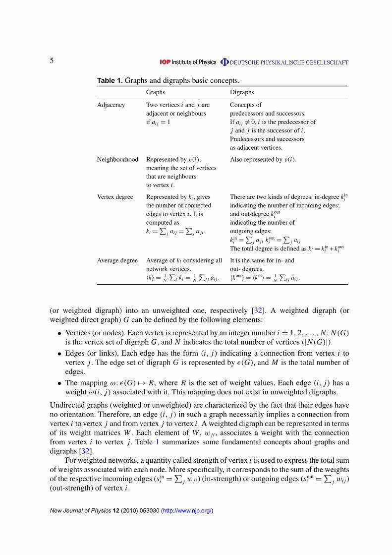
(or weighted digraph) into an unweighted one, respectively [32]. A weighted digraph (orweighted direct graph) G can be defined by the following elements:
• Vertices (or nodes). Each vertex is represented by an integer number i = 1, 2, . . . , N ; N (G)
is the vertex set of digraph G, and N indicates the total number of vertices (|N (G)|).
• Edges (or links). Each edge has the form (i, j) indicating a connection from vertex i tovertex j . The edge set of digraph G is represented by ε(G), and M is the total number ofedges.
• The mapping ω: ε(G) 7→ R, where R is the set of weight values. Each edge (i, j) has aweight ω(i, j) associated with it. This mapping does not exist in unweighted digraphs.
Undirected graphs (weighted or unweighted) are characterized by the fact that their edges haveno orientation. Therefore, an edge (i, j) in such a graph necessarily implies a connection fromvertex i to vertex j and from vertex j to vertex i . A weighted digraph can be represented in termsof its weight matrices W . Each element of W , w j i , associates a weight with the connectionfrom vertex i to vertex j . Table 1 summarizes some fundamental concepts about graphs anddigraphs [32].
For weighted networks, a quantity called strength of vertex i is used to express the total sumof weights associated with each node. More specifically, it corresponds to the sum of the weightsof the respective incoming edges (s in
i =∑
j w j i ) (in-strength) or outgoing edges (souti =
∑j wi j )
(out-strength) of vertex i .
New Journal of Physics 12 (2010) 053030 (http://www.njp.org/)
Another interesting measurement of local connectivity is the clustering coefficient. Thisfeature reflects the cyclic structure of networks, i.e. if they have a tendency to form sets ofdensely connected vertices. For digraphs, one way to calculate the clustering coefficient is: letmi be the number of neighbours of vertex i and li be the number of connections between theneighbours of vertex i ; the clustering coefficient is obtained as cc(i)= li/mi(mi − 1).
2.2. Data description
In this work, four music genres were selected: blues, bossa nova, reggae and rock. Thesegenres are well known and represent distinct major tendencies. Music samples belonging tothese genres are available in many collections in the Internet, so it was possible to select 100samples to represent each one of them. These samples were downloaded in MIDI format. This,event-like format contains instructions (such as notes, instruments, timbres and rhythms, amongothers), which are used by a synthesizer during the creation of new musical events [33]. TheMIDI format can be considered a digital musical score in which the instruments are separatedinto voices. Each sample in the dataset belongs to a single genre, since, in general, most MIDIdatabases found in the Internet are still single labelled.
In order to edit and analyse the MIDI scores, we applied the software for music compositionand notation called Sibelius (http://www.sibelius.com). For each sample, the voice related to thepercussion was extracted. The percussion is inherently suitable to express the rhythm of a piece.Once the rhythm is extracted, it becomes possible to analyse all the involved elements. TheMIDI Toolbox for Matlab was used in the present work [34]. This toolbox is free and containsfunctions to analyse and visualize MIDI files in the Matlab computing environment. Whena MIDI file is read with this toolbox, a matrix representation of note events is created. Thecolumns in this matrix refer to many types of information, such as: onset (in beats), duration(in beats), MIDI channel, MIDI pitch, velocity, onset (in seconds) and duration (in seconds). Therows refer to the individual note events, that is, each note is described in terms of its duration,pitch and so on.
Only the note duration (in beats) has been used in the current work. In fact, the durationsof the notes, respecting the sequence in which they occur in the sample, are used to create adigraph. Each vertex of this digraph represents one possible rhythm notation, such as quarternote, half note, eighth note and so on. The edges reflect the subsequent pairs of notes. Forexample, if there is an edge from vertex i , represented by a quarter note, to a vertex j ,represented by an eighth note, this means that a quarter note was followed by an eighth note atleast once. The thicker the edges, the larger is the strength between these two nodes. Examplesof these digraphs are shown in figure 1. Figure 1(a) depicts a blues sample represented by themusic How Blue Can You Get by BB King. A bossa nova sample, namely the music Fotografiaby Tom Jobim, is illustrated in 1(b). Figure 1(c) illustrates a reggae sample, represented by themusic Is This Love by Bob Marley. Finally, figure 1(d) shows a rock sample, corresponding tothe music From Me to You by the Beatles.
2.3. Feature extraction
Extracting features is the first step of most pattern recognition systems. Each pattern isrepresented by its d features or attributes in terms of a vector in a d-dimensional space. In adiscrimination problem, the goal is to choose features that allow the pattern vectors belonging
New Journal of Physics 12 (2010) 053030 (http://www.njp.org/)
Figure 1. Digraph examples of four music samples: (a) How Blue Can You Getby BB King. (b) fotografia by Tom Jobim. (c) Is This Love by Bob Marley.(d) From Me to You by The Beatles.
to different classes to occupy compact and distinct regions in the feature space, maximizingclass separability. After extracting significant features, any classification scheme may be used.In the case of music, features may belong to the main dimensions of music including melody,timbre, rhythm and harmony.
Therefore, one of the main features of this work is to extract features from the digraphsand use them to analyse the complexities of the rhythms, as well as to perform classificationtasks. For each sample, a digraph is created as described in the previous section. All digraphshave 18 nodes, corresponding to the quantity of rhythm notation possibilities concerning allthe samples, after excluding those that hardly ever happen. This exclusion was important inorder to provide an appropriate visual analysis and to better fit the features. In fact, avoidingfeatures that do not significantly contribute to the analysis reduces data dimensionality, improvesthe classification performance through a more stable representation and removes redundant orirrelevant information (in this case, minimizes the occurrence of null values in the data matrix).
The features are associated with the weight matrix W . As commented on in section 2.1,each element in W , wi j , indicates the weight of the connection from vertex j to i or, in other
New Journal of Physics 12 (2010) 053030 (http://www.njp.org/)
Figure 2. Block diagram of the proposed methodology.
words, they are meant to represent how often the rhythm notations follow one another in thesample. The weight matrix W has 18 rows and 18 columns. The matrix W is reshaped bya 1× 324 feature vector. This is done for each one of the genre samples. However, it wasobserved that some samples, even belonging to different genres, generated exactly the sameweight matrix. These samples were excluded. Thereby, the feature matrix has 280 rows (allnon-excluded samples) and 324 columns (the attributes).
An overview of the proposed methodology is illustrated in figure 2. After extractingthe features, a standardization transformation is done to guarantee that the new feature sethas zero mean and unit standard deviation. This procedure can significantly improve theresulting classification. Once the normalized features are available, the structure of the extractedrhythms can be analysed by using two different approaches for features analysis: principalcomponents analysis (PCA) and linear discriminant analysis (LDA). We also compare twotypes of classification methods: Bayesian classifier (supervised) and hierarchical clustering(unsupervised). PCA and LDA are described in section 2.4 and the classification methods aredescribed in section 2.5.
2.4. Feature analysis and redundancy removal
Two techniques are widely used for feature analysis [7, 35, 36]: PCA and LDA. Basically,these approaches apply geometric transformations (rotations) to the feature space with thepurpose of generating new features based on linear combinations of the original ones, aiming
New Journal of Physics 12 (2010) 053030 (http://www.njp.org/)
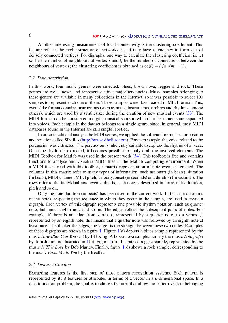
Figure 3. An illustration of PCA (optimizing representation) and LDAprojections (optimizing classification), adapted from [37].
at dimensionality reduction (in the case of PCA) or to seek a projection that best separates thedata (in the case of LDA). Figure 3 illustrates the basic principles underlying PCA and LDA.The direction x ′ (obtained with PCA) is the best one to represent the two classes with maximumoverall dispersion. However, it can be observed that the densities projected along direction x ′
overlap one another, making these two classes inseparable. In contrast, if direction y′, obtainedwith LDA, is chosen, the classes can be easily separated. Therefore, it is said that the directionsfor representation are not always also the best choice for classification, reflecting the differentobjectives of PCA and LDA [37]. Appendices A.1 and A.2 give more details of these twotechniques.
2.5. Classification methodology
Basically, to classify means to assign objects to classes or categories according to the propertiesthey present. In this context, the objects are represented by attributes, or feature vectors. Thereare three main types of pattern classification tasks: imposed criteria, supervised classification,and unsupervised classification. Imposed criteria are the easiest situation in classification, oncethe classification criteria is clearly defined, generally by a specific practical problem. If theclasses are known in advance, the classification is said to be supervised classification or byexample classification, since usually examples (the training set) are available for each class.Generally, supervised classification involves two stages: learning, in which the features aretested in the training set; and application, when new entities are presented to the trained system.There are many approaches involving supervised classification. The current study applies theBayesian classifier through discriminant functions (appendix B) in order to perform supervisedclassification. The Bayesian classifier is based on the Bayesian decision theory and combinesclass conditional probability densities (likelihood) and prior probabilities (prior knowledge) toperform classification by assigning each object to the class with the maximum a posterioriprobability.
In unsupervised classification, the classes are not known in advance, and there is not atraining set. This type of classification is usually called clustering, in which the objects areagglomerated according to some similarity criterion. The basic principle is to form classes orclusters so that the similarity between the objects in each class is maximized and the similaritybetween objects in different classes is minimized. There are two types of clustering: partitional(also called non-hierarchical) and hierarchical. In the former, a fixed number of clusters is
New Journal of Physics 12 (2010) 053030 (http://www.njp.org/)
obtained as a single partition of the feature space. Hierarchical clustering procedures are morecommonly used because they are usually simpler [6, 7, 36, 38]. The main difference is thatinstead of one definite partition, a series of partitions are taken, which is done progressively.If the hierarchical clustering is agglomerative (also known as bottom-up), the procedure startswith N objects as N clusters and then successively merges the clusters until all the objectsare joined into a single cluster (please refer to appendix C for more details of agglomerativehierarchical clustering). Divisive hierarchical clustering (top-down) starts with all the objects asa single cluster and splits it into progressively finer subclusters.
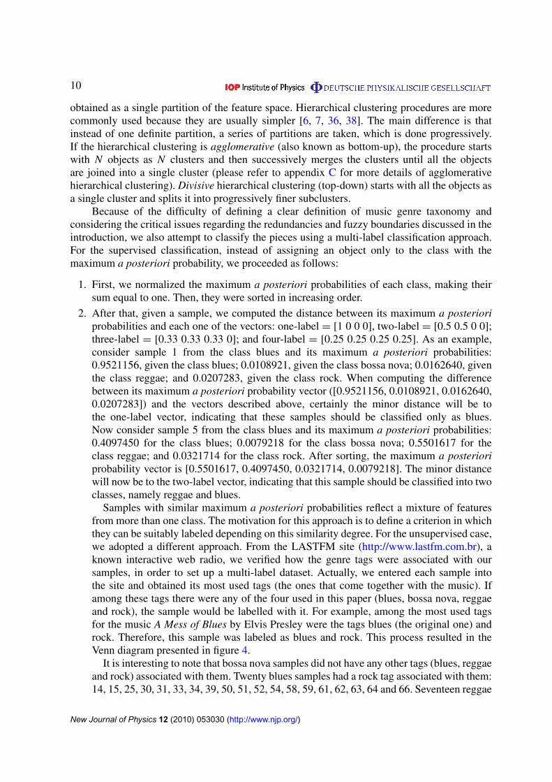
Because of the difficulty of defining a clear definition of music genre taxonomy andconsidering the critical issues regarding the redundancies and fuzzy boundaries discussed in theintroduction, we also attempt to classify the pieces using a multi-label classification approach.For the supervised classification, instead of assigning an object only to the class with themaximum a posteriori probability, we proceeded as follows:
1. First, we normalized the maximum a posteriori probabilities of each class, making theirsum equal to one. Then, they were sorted in increasing order.
2. After that, given a sample, we computed the distance between its maximum a posterioriprobabilities and each one of the vectors: one-label = [1 0 0 0], two-label = [0.5 0.5 0 0];three-label = [0.33 0.33 0.33 0]; and four-label = [0.25 0.25 0.25 0.25]. As an example,consider sample 1 from the class blues and its maximum a posteriori probabilities:0.9521156, given the class blues; 0.0108921, given the class bossa nova; 0.0162640, giventhe class reggae; and 0.0207283, given the class rock. When computing the differencebetween its maximum a posteriori probability vector ([0.9521156, 0.0108921, 0.0162640,0.0207283]) and the vectors described above, certainly the minor distance will be tothe one-label vector, indicating that these samples should be classified only as blues.Now consider sample 5 from the class blues and its maximum a posteriori probabilities:0.4097450 for the class blues; 0.0079218 for the class bossa nova; 0.5501617 for theclass reggae; and 0.0321714 for the class rock. After sorting, the maximum a posterioriprobability vector is [0.5501617, 0.4097450, 0.0321714, 0.0079218]. The minor distancewill now be to the two-label vector, indicating that this sample should be classified into twoclasses, namely reggae and blues.
Samples with similar maximum a posteriori probabilities reflect a mixture of featuresfrom more than one class. The motivation for this approach is to define a criterion in whichthey can be suitably labeled depending on this similarity degree. For the unsupervised case,we adopted a different approach. From the LASTFM site (http://www.lastfm.com.br), aknown interactive web radio, we verified how the genre tags were associated with oursamples, in order to set up a multi-label dataset. Actually, we entered each sample intothe site and obtained its most used tags (the ones that come together with the music). Ifamong these tags there were any of the four used in this paper (blues, bossa nova, reggaeand rock), the sample would be labelled with it. For example, among the most used tagsfor the music A Mess of Blues by Elvis Presley were the tags blues (the original one) androck. Therefore, this sample was labeled as blues and rock. This process resulted in theVenn diagram presented in figure 4.
It is interesting to note that bossa nova samples did not have any other tags (blues, reggaeand rock) associated with them. Twenty blues samples had a rock tag associated with them:14, 15, 25, 30, 31, 33, 34, 39, 50, 51, 52, 54, 58, 59, 61, 62, 63, 64 and 66. Seventeen reggae
New Journal of Physics 12 (2010) 053030 (http://www.njp.org/)
Figure 4. Venn diagram for the multi-label dataset.
samples also had a rock tag associated with them: 141, 142, 143, 159, 168, 172, 173, 174,176, 177, 178, 195, 199, 200, 201, 202 and 203. Finally, three rock samples had a blues tagassociated with them: 227, 228 and 276.
2.5.1. Performance measures for classification. To objectively evaluate the performance ofthe supervised classification, it is necessary to use quantitative criteria. The most used criteriaare the estimated classification error and the obtained accuracy. Because of its good statisticalproperties, such as, for example, being asymptotically normal with well-defined expressions toestimate its variances, this study also adopted the Cohen kappa coefficient [39] as a quantitativemeasure to analyse the performance of the proposed method. Besides, the kappa coefficient canbe directly obtained from the confusion matrix [40] (appendix D), easily computed in supervisedclassification problems. The confusion matrix is defined as
C =
c11 c12 . . . c1c
c21. . .
......
. . .
cc1 . . . ccc
, (1)
where each element ci j represents the number of objects from class i classified as class j .Therefore, the elements in the diagonal indicate the number of correct classifications.
We computed the performance of the multi-label and single unsupervised classifications,taking into consideration the following criterion: Performance= ni/Ni , where ni is the numberof correct classifications of class i and Ni is the number of samples of class i .
3. Results and discussion
As mentioned earlier, four musical genres were used in this study: blues, bossa nova, reggae androck. We selected music art works from diverse artists, as presented in tables 2 and 3. Differentcolors were chosen to represent the genres (the color red for the genre blues, green for bossanova, cyan for reggae and pink for rock) in order to provide a better visualization and discussionof the results.
New Journal of Physics 12 (2010) 053030 (http://www.njp.org/)
1. Albert Collins—A Good Fool 71. Antonio Adolfo—Sa Marina2. Albert Collins—Fake ID 72. Barquinho3. Albert King—Stormy Monday 73. Caetano Veloso—Menino Do Rio4. Andrews Sister—Boogie Woogie Bugle Boy 74. Caetano Veloso—Sampa5. B B King—Dont Answer The Door 75. Celso Fonseca—Ela E Carioca6. B B King—Get Off My Back 76. Celso Fonseca—Slow Motion bossa nova7. B B King—Good Time 77. Chico Buarque Els Soares—Facamos8. B B King—How Blue Can You Get 78. Chico Buarque Francis Hime—Meu Caro Amigo9. B B King—Sweet Sixteen 79. Chico Buarque Quarteto Em Si—Roda Viva
10. B B King—The Thrill Is Gone 80. Chico Buarque—As Vitrines11. B B King—Woke Up This Morning 81. Chico Buarque—Construcao12. Barbra Streisand—Am I Blue 82. Chico Buarque—Desalento13. Billie Piper—Something Deep Inside 83. Chico Buarque—Homenagem Ao Malandro14. Blues In F For Monday 84. Chico Buarque—Mulheres De Athenas15. Bo Diddley—Bo Diddley 85. Chico Buarque—Ole Ola16. Boy Williamson—Dont Start Me Talking 86. Chico Buarque—Sem Fantasia17. Boy Williamson—Help Me 87. Chico Buarque—Vai Levando18. Boy Williamson—Keep It To Yourself 88. Dick Farney—Copacabana19. Buddy Guy—Midnight Train 89. Elis Regina—Alo Alo Marciano20. Charlie Parker—Billies Bounce 90. Elis Regina—Como Nossos Pais21. Count Basie—Count On The Blues 91. Elis Regina—Na Batucada Da Vida22. Cream—Crossroads Blues 92. Elis Regina—O Bebado E O Equilibrista23. Delmore Brothers—Blues Stay Away From Me 93. Elis Regina—Romaria24. Elmore James—Dust My Broom 94. Elis Regina—Velho Arvoredo25. Elvis Presley—A Mess Of Blues 95. Emilio Santiago—Essa Fase Do Amor26. Etta James—At Last 96. Emilio Santiago—Esta Tarde Vi Voller27. Feeling The Blues 97. Emilio Santiago—Saigon28. Freddie King—Help Day 98. Emilio Santiago—Ta Tudo Errado29. Freddie King—Hide Away 99. Gal Costa—Canta Brasil30. Gary Moore—A Cold Day In Hell 100. Gal Costa—Para Machucar Meu Coracao31. George Thorogood—Bad To The Bone 101. Gal Costa—Pra Voce32. Howlin Wolf—Little Red Rooster 102. Gal Costa—Um Dia De Domingo33. Janis Joplin—Piece Of My Heart 103. Jair Rodrigues—Disparada34. Jimmie Cox—Before You Accuse Me 104. Joao Bosco—Corsario35. Jimmy Smith—Chicken Shack 105. Joao Bosco—De Frente Para O Crime36. John Lee Hooker—Boom Boom Boom 106. Joao Bosco—Jade37. John Lee Hooker—Dimples 107. Joao Bosco—Risco De Giz38. John Lee Hooker—One Bourbon One Scotch One Beer 108. Joao Gilberto—Corcovado39. Johnny Winter—Good Morning Little School Girl 109. Joao Gilberto—Da Cor Do Pecado40. Koko Taylor—Hey Bartender 110. Joao Gilberto—Um Abraco No Bonfa41. Little Walter—Juke 111. Luiz Bonfa—De Cigarro Em Cigarro42. Louis Jordan—Let Good Times Roll 112. Luiz Bonfa—Manha De Carnaval43. Miles Davis—All Blues 113. Marcos Valle—Preciso Aprender A Viver So44. Ray Charles—Born To The Blues 114. Marisa Monte—Ainda Lembro45. Ray Charles—Crying Time 115. Marisa Monte—Amor I Love You46. Ray Charles—Georgia On My Mind 116. Marisa Monte—Ando Meio Desligado
New Journal of Physics 12 (2010) 053030 (http://www.njp.org/)
47. Ray Charles—Hit The Road Jack 117. Tom Jobim—Aguas De Marco48. Ray Charles—Unchain My Heart 118. Tom Jobim—Amor Em Paz49. Robert Johnson—Dust My Broom 119. Tom Jobim—Brigas Nunca Mais50. Stevie Ray Vaughan—Cold Shot 120. Tom Jobim—Desafinado51. Stevie Ray Vaughan—Couldnt Stand The Weather 121. Tom Jobim—Fotografia52. Stevie Ray Vaughan—Dirty Pool 122. Tom Jobim—Garota De Ipanema53. Stevie Ray Vaughan—Hillbillies From Outer Space 123. Tom Jobim—Meditacao54. Stevie Ray Vaughan—I Am Crying 124. Tom Jobim—Samba Do Aviao55. Stevie Ray Vaughan—Lenny 125. Tom Jobim—Se Todos Fossem Iguais A Voce56. Stevie Ray Vaughan—Little Wing 126. Tom Jobim—So Tinha De Ser Com Voce57. Stevie Ray Vaughan—Looking Out The Window 127. Tom Jobim—Vivo Sonhando58. Stevie Ray Vaughan—Love Struck Baby 128. Tom Jobim—Voce Abusou59. Stevie Ray Vaughan—Manic Depression 129. Tom Jobim—Wave60. Stevie Ray Vaughan—Scuttle Buttin 130. Toquinho—Agua Negra Da Lagoa61. Stevie Ray Vaughan—Superstition 131. Toquinho—Ao Que Vai62. Stevie Ray Vaughan—Tell Me 132. Toquinho—Este Seu Olhar63. Stevie Ray Vaughan—Voodoo Chile 133. Vinicius De Moraes—Apelo64. Stevie Ray Vaughan—Wall Of Denial 134. Vinicius De Moraes—Carta Ao Tom65. T Bone Walker—Call It Stormy Monday 135. Vinicius De Moraes—Minha Namorada66. The Blues Brothers—Everybody Needs Somebody To Love 136. Vinicius De Moraes—O Morro Nao Tem Vez67. The Blues Brothers—Green Onions 137. Vinicius De Moraes—Onde Anda Voce68. The Blues Brothers—Peter Gunn Theme 138. Vinicius De Moraes—Pela Luz Dos Olhos Teus69. The Blues Brothers—Soulman 139. Vinicius De Moraes—Samba Em Preludio70. W C Handy—Memphis Blues 140. Vinicius De Moraes—Tereza Da Praia
3.1. Single classification results
If we want to reduce data dimensionality, it is necessary to set a suitable number of principalcomponents that will represent the new features. Not surprisingly, in a high dimensional space,the classes can be easily separated. On the other hand, high dimensionality increases complexity,making the analysis of both extracted features and classification results a difficult task. Oneapproach to obtain the ideal number of principal components is to verify how much of the datavariance is preserved. In order to do so, the l first eigenvalues (l is the quantity of principalcomponents to be verified) are summed up and the result is divided by the sum of all theeigenvalues. If the result of this calculation is a value equal to or greater than 0.75, it is said thatthis number of components (or new features) preserves at least 75% of the data variance, whichis often enough for classification purposes. When PCA was applied to the normalized rhythmfeatures, as illustrated in figure 5, it was observed that 15 principal components preserved 76%of the variance of the data. That is, it is possible to reduce the data dimensionality from 364-D to15-D without a significant loss of information. Nevertheless, as will be shown in the following,depending on the classifier and how the classification task was performed, different numbersof components were required in each situation in order to achieve suitable results. Althoughpreserving only 36% of the variance, figure 5 shows the first three principal components, thatis, the first three new features obtained with PCA. Figure 5(a) shows the first and second
New Journal of Physics 12 (2010) 053030 (http://www.njp.org/)
141. Ace Of Bass—All That She Wants 211. Aerosmith—Kings And Queens142. Ace Of Bass—Dont Turn Around 212. Aha—Stay On These Roads143. Ace Of Bass—Happy Nation 213. Aha—Take On Me144. Armandinho—Pela Cor Do Teu Olho 214. Aha—Theres Never A Forever Thing145. Armandinho—Sentimento 215. Beatles—Cant Buy Me Love146. Big Mountain—Baby I Love Your Way 216. Beatles—From Me To You147. Bit Mclean—Be Happy 217. Beatles—I Want To Hold Your Hand148. Bob Marley—Africa Unite 218. Beatles—She Loves You149. Bob Marley—Buffalo Soldier 219. Billy Idol—Dancing With Myself150. Bob Marley—Exodus 220. Cat Stevens—Another Saturday Night151. Bob Marley—Get Up, Stand Up 221. Creed—My Own Prison152. Bob Marley—I Shot The Sheriff 222. Deep Purple—Demon Eye153. Bob Marley—Iron Lion Zion 223. Deep Purple—Hallelujah154. Bob Marley—Is This Love 224. Deep Purple—Hush155. Bob Marley—Jammin 225. Dire Straits—Sultan Of Swing156. Bob Marley—No Woman No Cry 226. Dire Straits—Walk Of Life157. Bob Marley—Punky Reggae Party 227. Duran Duran—A View To A Kill158. Bob Marley—Root, Rock, Reggae 228. Eric Clapton—Cocaine159. Bob Marley—Satisfy my soul 229. Europe—Carrie160. Bob Marley—Stir It Up 230. Fleetwood Mac—Dont Stop161. Bob Marley—Three Little Birds 231. Fleetwood Mac—Dreams162. Bob Marley—Waiting In The Van 232. Fleetwood Mac—Gold Dust Woman163. Bob Marley—War 233. Foo Fighters—Big Me164. Bob Marley—Wear My 234. Foo Fighters—Break Out165. Bob Marley—Zimbabwe 235. Foo Fighters—Walking After You166. Cidade Negra—A Cor Do Sol 236. Men At Work—Down Under167. Cidade Negra—A Flecha E O Vulcao 237. Men At Work—Who Can It Be Now168. Cidade Negra—A Sombra Da Maldade 238. Metallica—Battery169. Cidade Negra—Aonde Voce Mora 239. Metallica—Fuel170. Cidade Negra—Eu Fui Eu Fui 240. Metallica—Hero Of The Day171. Cidade Negra—Eu Tambem Quero Beijar 241. Metallica—Master Of Puppets172. Cidade Negra—Firmamento 242. Metallica—My Friend of Misery173. Cidade Negra—Girassol 243. Metallica—No Leaf Clover174. Cidade Negra—Ja Foi 244. Metallica—One175. Cidade Negra—Mucama 245. Metallica—Sad But True176. Cidade Negra—O Ere 246. Pearl Jam—Alive177. Cidade Negra—Pensamento 247. Pearl Jam—Black178. Dazaranhas—Vagabundo Confesso 248. Pearl Jam—Jeremy179. Dont Worry 249. Pet Shop Boys—Go West180. Flor Do Reggae 250. Pet Shop Boys—One In A Million181. Inner Circle—Bad Boys 251. Pink Floyd—Astronomy Domine182. Inner Circle—Sweat 252. Pink Floyd—Have A Cigar183. Jimmy Cliff—I Can See Clearly Now 253. Pink Floyd—Hey You184. Jimmy Cliff—Many Rivers To Cross 254. Queen—Another One Bites The Dust185. Jimmy Cliff—Reggae Night 255. Queen—Dont Stop Me Now186. Keep On Moving 256. Queen—I Want It All
New Journal of Physics 12 (2010) 053030 (http://www.njp.org/)
187. Manu Chao—Me Gustas Tu 257. Queen—Play The Game188. Maskavo—Anjo Do Ceu 258. Queen—Radio Gaga189. Maskavo—Asas 259. Queen—Under Pressure190. Natiruts—Liberdade Pra Dentro Da Cabeca 260. Red Hot Chili Peppers—Higher Ground191. Natiruts—Presente De Um Beija Flor 261. Red Hot Chili Peppers—Otherside192. Natiruts—Reggae Power 262. Red Hot Chili Peppers—Under The Bridge193. Nazarite Skank 263. Rolling Stones—Angie194. Peter Tosh—Johnny B Goode 264. Rolling Stones—As Tears Go By195. Shaggy—Angel 265. Rolling Stones—Satisfaction196. Shaggy—Bombastic 266. Rolling Stones—Street Of Love197. Shaggy—It Wasnt Me 267. Steppenwolf—Magic Carpet Ride198. Shaggy—Strength Of A Woman 268. Steve Winwood—Valerie199. Sublime—Badfish 269. Steve Winwood—While You See A Chance200. Sublime—D. Js 270. Tears For Fears—Shout201. Sublime—Santeria 271. The Doors—Hello, I Love You202. Sublime—Wrong Way 272. The Doors—Light My Fire203. Third World—Now That We Found Love 273. The Doors—Love Her Madly204. Tribo De Jah—Babilonia Em Chamas 274. U2—Elevation205. Tribo De Jah—Regueiros Guerreiros 275. U2—Everlasting Love206. Tribo De Jah—Um So Amor 276. U2—When Love Comes To Town207. UB 40—Bring Me Your Cup 277. Van Halen—Dance The Night Away208. UB 40—Homely Girl 278. Van Halen—Running With The Devil209. UB 40—To Love Somebody 279. Van Halen—Jump210. UB 40—Red Red Wine 280. Van Halen—Panama
−1.5 −1.0 −0.5 0.0 0.5 1.0 1.5 2.0−1.0
−0.5
0.0
0.5
1.0
1.5
First component
Sec
ond
com
pone
nt
Blues
Bossa nova
Reggae
Rock
(a)
−1.5 −1.0 −0.5 0.0 0.5 1.0 1.5 2.0−1.5
−1.0
−0.5
0.0
0.5
1.0
First component
Thi
rd c
ompo
nent
Blues
Bossa nova
Reggae
Rock
(b)
Figure 5. The first three new features obtained by PCA. (a) The first and secondaxes. (b) The first and third axes.
features and figure 5(b) shows the first and third features. It should be noted that the classesare completely overlapping, making the problem of automatic classification a nontrivial task.
In all the following supervised classification tasks, re-substitution means that all objectsfrom each class were used as the training set (in order to estimate the parameters) and all objects
New Journal of Physics 12 (2010) 053030 (http://www.njp.org/)
were used as the testing set. Hold-out 70–30% means that 70% of the objects from each classwere used as the training set and 30% (different ones) for testing. Finally, in hold-out 50–50%,the objects were separated into two groups: 50% for training and 50% for testing.
The kappa variance is strongly related to its accuracy, that is, how reliable are its values.The higher its variance, the lower its accuracy. If the kappa coefficient is a statistics, in general,the use of large datasets improves its accuracy by making its variance smaller. This can beobserved in the results. The smaller variance occurred in the re-substitution situation, in whichall samples constitute the testing set. This indicates that re-substitution provided the best kappaaccuracy in the experiments. On the other hand, hold-out 70–30% provided higher kappavariance, if only 30% of the samples establish the testing set.
The results obtained by the quadratic Bayesian classifier using PCA are shown in table 4in terms of kappa, its variance, the accuracy of the classification and the overall performanceaccording to the value of kappa.
Table 4 also indicates that the performance was not satisfactory for the hold-out 70–30%and hold-out 50–50%. As PCA is not a supervised approach, the parameter estimationperformance (of covariance matrices for instance) is strongly degraded because of the smallsample size problem.
The confusion matrix for the re-substitution classification task in table 4 is illustrated intable 5. All reggae samples were classified correctly. In addition, many samples from the otherclasses were classified as reggae.
New Journal of Physics 12 (2010) 053030 (http://www.njp.org/)
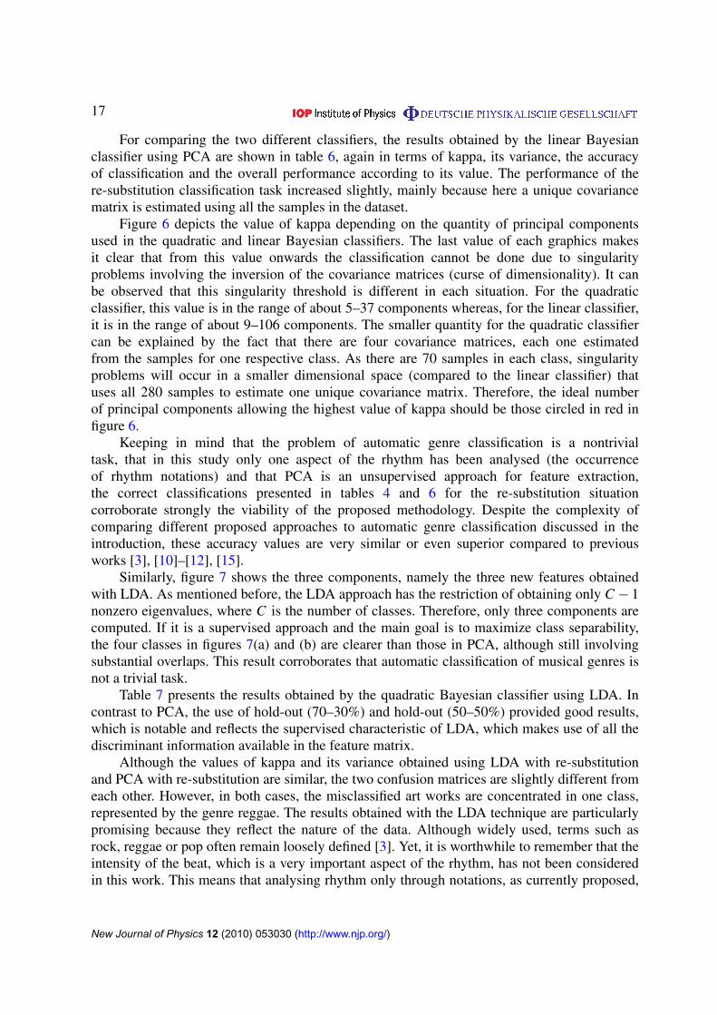
For comparing the two different classifiers, the results obtained by the linear Bayesianclassifier using PCA are shown in table 6, again in terms of kappa, its variance, the accuracyof classification and the overall performance according to its value. The performance of there-substitution classification task increased slightly, mainly because here a unique covariancematrix is estimated using all the samples in the dataset.
Figure 6 depicts the value of kappa depending on the quantity of principal componentsused in the quadratic and linear Bayesian classifiers. The last value of each graphics makesit clear that from this value onwards the classification cannot be done due to singularityproblems involving the inversion of the covariance matrices (curse of dimensionality). It canbe observed that this singularity threshold is different in each situation. For the quadraticclassifier, this value is in the range of about 5–37 components whereas, for the linear classifier,it is in the range of about 9–106 components. The smaller quantity for the quadratic classifiercan be explained by the fact that there are four covariance matrices, each one estimatedfrom the samples for one respective class. As there are 70 samples in each class, singularityproblems will occur in a smaller dimensional space (compared to the linear classifier) thatuses all 280 samples to estimate one unique covariance matrix. Therefore, the ideal numberof principal components allowing the highest value of kappa should be those circled in red infigure 6.
Keeping in mind that the problem of automatic genre classification is a nontrivialtask, that in this study only one aspect of the rhythm has been analysed (the occurrenceof rhythm notations) and that PCA is an unsupervised approach for feature extraction,the correct classifications presented in tables 4 and 6 for the re-substitution situationcorroborate strongly the viability of the proposed methodology. Despite the complexity ofcomparing different proposed approaches to automatic genre classification discussed in theintroduction, these accuracy values are very similar or even superior compared to previousworks [3], [10]–[12], [15].
Similarly, figure 7 shows the three components, namely the three new features obtainedwith LDA. As mentioned before, the LDA approach has the restriction of obtaining only C − 1nonzero eigenvalues, where C is the number of classes. Therefore, only three components arecomputed. If it is a supervised approach and the main goal is to maximize class separability,the four classes in figures 7(a) and (b) are clearer than those in PCA, although still involvingsubstantial overlaps. This result corroborates that automatic classification of musical genres isnot a trivial task.
Table 7 presents the results obtained by the quadratic Bayesian classifier using LDA. Incontrast to PCA, the use of hold-out (70–30%) and hold-out (50–50%) provided good results,which is notable and reflects the supervised characteristic of LDA, which makes use of all thediscriminant information available in the feature matrix.
Although the values of kappa and its variance obtained using LDA with re-substitutionand PCA with re-substitution are similar, the two confusion matrices are slightly different fromeach other. However, in both cases, the misclassified art works are concentrated in one class,represented by the genre reggae. The results obtained with the LDA technique are particularlypromising because they reflect the nature of the data. Although widely used, terms such asrock, reggae or pop often remain loosely defined [3]. Yet, it is worthwhile to remember that theintensity of the beat, which is a very important aspect of the rhythm, has not been consideredin this work. This means that analysing rhythm only through notations, as currently proposed,
New Journal of Physics 12 (2010) 053030 (http://www.njp.org/)
could pose difficulties, even for human experts. These misclassified art works have similarproperties described in terms of rhythm notations and, as a result, they generate similar weightmatrices. Therefore, the proposed methodology, although requiring some complementation,seems to be a significant contribution toward the development of a viable alternative approachto automatic genre classification.
The results for the linear Bayesian classifier using LDA are shown in table 9. In fact, theyare closely similar to those obtained by the quadratic Bayesian classifier (table 7).
New Journal of Physics 12 (2010) 053030 (http://www.njp.org/)
As mentioned in appendix A.2, LDA also allows us to quantify the intra- and interclassdispersion of the feature matrix through functionals such as the trace and determinant computedfrom the scatter matrices [41]. The overall intraclass scatter matrix, denoted Sintra; the intraclassscatter matrix for each class, denoted SintraBlues, SintraBossaNova, SintraReggae and SintraRock; theinterclass scatter matrix, denoted, Sinter; and the overall separability index, denoted (S−1
intra ∗ Sinter),were computed. Their respective traces are
trace(Sintra)= 505.55,
trace(SintraBlues)= 154.96,
trace(SintraBossaNova)= 127.41,
trace(SintraReggae)= 91.76,
trace(SintraRock)= 131.40,
trace(Sinter)= 22.08,
trace(S−1intra ∗ Sinter)= 3.49.
Two important observations are worth mentioning. Firstly, these traces emphasize thedifficulty of this classification problem: the traces of the intraclass scatter matrices are too high,and the trace of the interclass scatter matrix together with the overall separability index, aretoo small. This confirms that the four classes are overlapping completely. Secondly, the smallerintra-class trace is related to the genre reggae (it is the most compact class). This may justifywhy, in the experiments, art works belonging to reggae were more frequently 90–100% correctlyclassified.
The PCA and LDA approaches help one to identify the features that contribute the mostto the classification. This is an interesting analysis that can be performed by verifying thestrength of each element in the first eigenvectors and then associating those elements withthe original features. Within the current study, it was figured out that the first ten sequencesof rhythm notations that contributed the most to separation correspond to those illustrated infigure 8. In the case of the first and second eigenvectors obtained by PCA and LDA, the tenelements with higher values were selected, and the indices of these elements were associatedwith the sequences in the original weight matrix. Figures 8(a) and (b) show the resultingsequences according to the first and second eigenvectors of PCA. The thickness of the edgesis set by the value of the corresponding element in the eigenvector. It is interesting that thesesequences are the ones that mostly frequently occur in the rhythms from all four genres studiedhere. That is, they correspond to the elements that play the greatest role in representing therhythms. Therefore, it can be said that these are the ten most representative sequences that thefirst and second eigenvectors of PCA take into account. Triples of the eighth and sixteenthnotes are particularly important in the genres blues and reggae. Similarly, figures 8(c) and(d) show the resulting sequences according to the first and second eigenvectors of LDA. Incontrast to those obtained by PCA, these sequences are not common to all the rhythms, butthey must occur with distinct frequency within each genre. Thus, they are referred to here asthe ten most discriminative sequences if the first and second eigenvectors of LDA are taken intoaccount.
Clustering results are discussed in the following. The number of clusters was defined asfour, in order to provide a fair comparison with the supervised classification results. The idea
New Journal of Physics 12 (2010) 053030 (http://www.njp.org/)
Figure 8. The ten most significant sequences of rhythm notations according to(a) the first PCA eigenvector, (b) the second PCA eigenvector, (c) the first LDAeigenvector and (d) the second LDA eigenvector.
behind the confusion matrix in table 10 is to verify how many art works from each class wereplaced in each one of the four clusters. For example, it is known that from 1 to 70 art worksbelong to the genre blues. Then, the first line of this confusion matrix indicates that 25 blues artworks were placed in cluster 1, 11 in cluster 2, 12 in cluster 3 and 22 in cluster 4. It can alsobe observed that in cluster 1, reggae art works are the majority (46), whereas in cluster 2, themajority are bossa nova art works (16), despite the small difference compared to the number of
New Journal of Physics 12 (2010) 053030 (http://www.njp.org/)
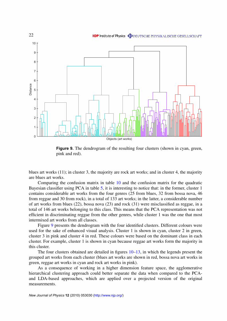
Figure 9. The dendrogram of the resulting four clusters (shown in cyan, green,pink and red).
blues art works (11); in cluster 3, the majority are rock art works; and in cluster 4, the majorityare blues art works.
Comparing the confusion matrix in table 10 and the confusion matrix for the quadraticBayesian classifier using PCA in table 5, it is interesting to notice that: in the former, cluster 1contains considerable art works from the four genres (25 from blues, 32 from bossa nova, 46from reggae and 30 from rock), in a total of 133 art works; in the latter, a considerable numberof art works from blues (22), bossa nova (23) and rock (31) were misclassified as reggae, in atotal of 146 art works belonging to this class. This means that the PCA representation was notefficient in discriminating reggae from the other genres, while cluster 1 was the one that mostintermixed art works from all classes.
Figure 9 presents the dendrogram with the four identified clusters. Different colours wereused for the sake of enhanced visual analysis. Cluster 1 is shown in cyan, cluster 2 in green,cluster 3 in pink and cluster 4 in red. These colours were based on the dominant class in eachcluster. For example, cluster 1 is shown in cyan because reggae art works form the majority inthis cluster.
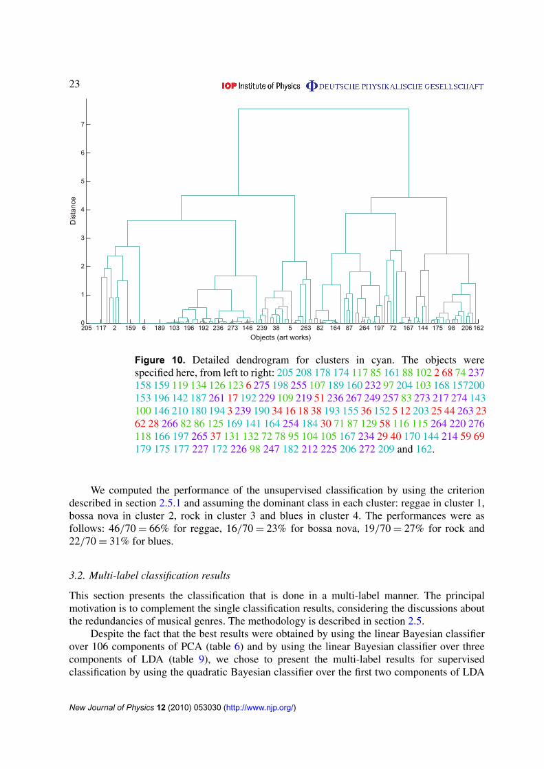
The four clusters obtained are detailed in figures 10–13, in which the legends present thegrouped art works from each cluster (blues art works are shown in red, bossa nova art works ingreen, reggae art works in cyan and rock art works in pink).
As a consequence of working in a higher dimension feature space, the agglomerativehierarchical clustering approach could better separate the data when compared to the PCA-and LDA-based approaches, which are applied over a projected version of the originalmeasurements.
New Journal of Physics 12 (2010) 053030 (http://www.njp.org/)
We computed the performance of the unsupervised classification by using the criteriondescribed in section 2.5.1 and assuming the dominant class in each cluster: reggae in cluster 1,bossa nova in cluster 2, rock in cluster 3 and blues in cluster 4. The performances were asfollows: 46/70= 66% for reggae, 16/70= 23% for bossa nova, 19/70= 27% for rock and22/70= 31% for blues.
3.2. Multi-label classification results
This section presents the classification that is done in a multi-label manner. The principalmotivation is to complement the single classification results, considering the discussions aboutthe redundancies of musical genres. The methodology is described in section 2.5.
Despite the fact that the best results were obtained by using the linear Bayesian classifierover 106 components of PCA (table 6) and by using the linear Bayesian classifier over threecomponents of LDA (table 9), we chose to present the multi-label results for supervisedclassification by using the quadratic Bayesian classifier over the first two components of LDA
New Journal of Physics 12 (2010) 053030 (http://www.njp.org/)
Figure 11. Detailed dendrogram for clusters in green. The objects were specifiedhere, from left to right: 8 9 32 26 79 10 260 21 147 80 56 150 202 218 76 230 139120 90 133 13 112 122 185 96 46 111 173 279 70 149 154 278 188 128 84 43259 94 113135 235 and 224.
(with kappa = 0.48), since this is easier to illustrate graphically. Tables 11 and 12 present theobtained labels for each sample. In order to provide a suitable and graphical visualization of suchresults, figure 14 shows the contour plots of the 2D class conditional Gaussian densities togetherwith the scatter plots of the dataset. The contour plots are obtained by defining equally spacedsubintervals within the range [pmin, pmax], where pmin is the minimum probability value and pmax
is the maximum probability value of the distribution. In our case, illustrated in figure 14, thecontour plots are given by the central isolines of such intervals (the ones that divide the interval[pmin, pmax] in two halves). It is possible to observe that the labels of each sample are relatedto their position in the feature space. As an example, consider the blues sample number 30.Although it is a blues sample, its features are more similar to those of the bossa nova samples,that is, its feature vector is located closer to the centre of the reggae conditional density thanto the centre of the blues density. Therefore, it is expected that this sample be classified asbelonging to the bossa nova class. Samples 56 and 265 were classified as belonging to the fourclasses. None of the reggae samples were classified as reggae only, since reggae and rock classconditional densities are almost completely overlapping.
The performance of the multi-label unsupervised classification results was computedconsidering the multi-label dataset presented in section 2.5. For example, instead of consideringonly the 19 rock samples in the rock cluster, we now verify how many of the 17 reggae–rocksamples and how many blues–rock samples there are in the rock cluster, since now they arealso referred to as rock samples. The new total of rock samples is 107. The performances
New Journal of Physics 12 (2010) 053030 (http://www.njp.org/)
Figure 12. Detailed dendrogram for clusters in pink. The objects were specifiedhere, from left to right: 4 19 269 55 238 136 110 251 199 280 50 61 245 244 52 5463 89 262 106 181 250 137 186 81 248 228 240 252 242 233 22 215 165 60 101268 73 121 130 108 148 271 195 277 124 127 140 216 39 and 66.
are: bossa nova—23%, since no blues, rock or reggae samples were also labelled as bossa nova;reggae—66%, since no blues, bossa nova or rock samples were also labelled as reggae;rock—26% ((19+2+7)/107), since two reggae–rock samples are in the rock cluster and sevenblues–rock samples are in the rock cluster; and blues—30% (22/73), since none of the threerock–blues samples are in the blues cluster.
4. Concluding remarks
Automatic music genre classification has become a fundamental topic in music research sincegenres have been widely used to organize and describe music collections. They also revealgeneral identities of different cultures. However, music genres are not a clearly defined conceptso that the development of a non-controversial taxonomy represents a challenging, nontrivialtask.
Generally speaking, music genres summarize common characteristics of musical pieces.This is particularly interesting when it is used as a resource for automatic classification of pieces.In the current paper, we explored genre classification taking into account the music’s temporalaspects, namely the rhythm. We considered pieces of four musical genres (blues, bossa nova,reggae and rock), which were extracted from MIDI files and modelled as networks. Each nodecorresponded to one rhythmic notation, and the links were defined by the sequence in whichthey occurred in time. The idea of using static nodes (nodes with fixed positions) is particularly
New Journal of Physics 12 (2010) 053030 (http://www.njp.org/)
Figure 13. Detailed dendrogram for clusters in red. The objects were specifiedhere, from left to right: 1 77 14 67 65 20 27 24 49 151 211 222 33 171 35 48 19191 183 92 270 223 7 42 114 176 207 201 221 163 243 246 256 241 253 11 21341 145 47 75 99 258 156 15 138 53 93 231 31 45 57 and 64.
interesting because it provides a primary visual identification of the differences and similaritiesbetween the rhythms from the four genres. A Markov model was built from the networks,and the dynamics and dependences of the rhythmic notations were estimated, comprising thefeature matrix of the data. Two different approaches for features analysis were used (PCAand LDA), as well as two types of classification methods (Bayesian classifier and hierarchicalclustering).
Using only the first two principal components of PCA, the different types of rhythms werenot separable, although for the first and third axes we could observe some separation betweenthree of the classes (blues, bossa nova and reggae), while only the samples of rock overlappedthe other classes. However, taking into account that 15 components were necessary to preserve76% of the data variance, it is expected that only two or three dimensions would not be sufficientto allow suitable separability. Notably, the dimensionality of the problem is high, that is, therhythms are very complex and many dimensions (features) are necessary to separate them.This is one of the main findings of the current work. With the help of LDA analysis, anotherfinding was reached, which supported the assumption that the problem of automatic rhythmclassification is no trivial task. The projections obtained by considering the first and second, andfirst and third axes implied better discrimination between the four classes than that obtained bythe PCA.
Unlike PCA and LDA, agglomerative hierarchical clustering works on the originaldimensions of the data. The application of the methodology led to a substantially better
New Journal of Physics 12 (2010) 053030 (http://www.njp.org/)
Table 11. Multi-label classification results over all blues and bossa nova samples.
Blues samples Bossa nova samples
1. blues 71. bossa nova2. reggae and rock 72. bossa nova3. reggae and blues 73. bossa nova4. blues 74. bossa nova, rock and reggae5. blues 75. bossa nova6. reggae and rock 76. reggae, bossa nova, and rock7. blues 77. bossa nova8. blues 78. bossa nova9. blues 79. bossa nova, rock and reggae
10. blues 80. rock11. blues 81. bossa nova12. blues 82. reggae, rock and bossa nova13. blues 83. reggae and rock14. blues 84. bossa nova15. blues 85. bossa nova, reggae and rock16. blues 86. reggae, rock and bossa nova17. reggae and rock 87. bossa nova18. blues 88. bossa nova19. blues 89. reggae, rock and blues20. blues 90. blues, reggae and rock21. blues 91. bossa nova22. blues 92. bossa nova23. blues 93. bossa nova24. blues 94. bossa nova25. blues 95. bossa nova26. blues 96. reggae, rock and bossa nova27. blues 97. reggae and rock28. reggae, rock and bossa nova 98. rock and reggae29. blues and reggae 99. bossa nova, rock and reggae30. bossa nova 100. reggae and rock31. blues 101. bossa nova32. blues 102. bossa nova33. blues 103. reggae and rock34. blues 104. bossa nova35. blues 105. bossa nova36. blues and reggae 106. reggae, rock and bossa nova37. rock, blues and bossa nova 107. reggae and rock38. blues 108. bossa nova39. blues 109. reggae and rock40. blues 110. bossa nova41. blues 111. reggae and rock42. blues 112. reggae, rock and bossa nova43. blues 113. bossa nova44. blues 114. bossa nova
New Journal of Physics 12 (2010) 053030 (http://www.njp.org/)
45. blues 115. reggae, rock and bossa nova46. blues 116. reggae, rock and blues47. blues 117. bossa nova, reggae and rock48. blues 118. reggae, rock and bossa nova49. blues 119. bossa nova50. blues 120. bossa nova51. reggae and rock 121. bossa nova52. blues, reggae and rock 122. reggae, rock and bossa nova53. blues 123. bossa nova54. reggae, blues and rock 124. bossa nova55. blues 125. reggae, rock and bossa nova56. reggae, rock, blues and bossa nova 126. bossa nova57. blues 127. bossa nova58. blues and reggae 128. bossa nova59. blues 129. bossa nova60. blues 130. bossa nova61. blues 131. bossa nova62. blues 132. bossa nova63. reggae, blues and rock 133. bossa nova64. blues 134. bossa nova65. blues 135. bossa nova66. blues 136. bossa nova67. blues 137. bossa nova68. blues 138. bossa nova69. rock and reggae 139. bossa nova70. blues 140. bossa nova
discrimination, which provides strong evidence of the complexity of the problem studied here.The results are promising in the sense that each cluster is dominated by a different genre,showing the viability of the proposed approach.
The use of a multi-label approach was interesting and particularly appropriate, since itreflected the intrinsic nature of the dataset. Musical genre classification is a nontrivial task evenfor music experts, since often a song can be assigned to more than a single genre. Automaticclassification is considerably more complex, because there are many samples with similarfeature vectors, defining huge overlapping areas in the feature space, as observed in our study. Inthis context, multi-label classification plays a fundamental role, making possible generalizationof the genre taxonomy, originally presented in the training set. With our proposed method,new sub-genres (for example, rock–blues) can arise from original ones. Therefore, we observeda significant improvement in the supervised classification performance. For the multi-labelunsupervised approach, which does not take the data covariance structure into account, we didnot observe significant changes in the classification performances. Furthermore, the labellingprocess that takes place in the LastFm website, through direct listener interaction, considersall music content (instruments, harmony, melody, pitch, voice and percussion, among others).
New Journal of Physics 12 (2010) 053030 (http://www.njp.org/)
Table 12. Multi-label classification results over all reggae and rock samples.
Reggae samples Rock samples
141. reggae, rock and bossa nova 211. rock142. rock and reggae 212. rock and reggae143. reggae and rock 213. rock144. blues 214. reggae and rock145. rock and reggae 215. rock146. reggae and rock 216. rock147. reggae, rock and bossa nova 217. reggae and rock148. reggae and rock 218. reggae, rock and bossa nova149. reggae, rock and bossa nova 219. reggae and rock150. reggae, bossa nova and rock 220. reggae, rock and bossa nova151. rock and reggae 221. rock152. blues and reggae 222. rock153. reggae and rock 223. rock154. reggae, blues and rock 224. rock155. blues and reggae 225. reggae and rock156. rock and reggae 226. rock and reggae157. reggae and rock 227. reggae and rock158. bossa nova, rock and reggae 228. rock159. bossa nova, rock and reggae 229. reggae and rock160. reggae and rock 230. reggae, bossa nova and rock161. reggae and rock 231. rock162. bossa nova 232. reggae and rock163. rock and reggae 233. rock164. reggae, rock and bossa nova 234. bossa nova165. rock and reggae 235. rock166. reggae, rock and bossa nova 236. reggae and rock167. bossa nova 237. bossa nova, rock and reggae168. reggae and rock 238. blues169. reggae, rock and bossa nova 239. blues and reggae170. blues 240. rock171. rock and reggae 241. rock172. rock and reggae 242. rock173. rock and reggae 243. rock174. bossa nova, reggae and rock 244. rock175. rock and reggae 245. blues and reggae176. reggae and rock 246. bossa nova, reggae and rock177. rock and reggae 247. rock and reggae178. bossa nova, reggae and rock 248. rock179. rock and reggae 249. reggae and rock180. reggae and rock 250. rock181. reggae, rock and bossa nova 251. rock182. rock and reggae 252. rock183. rock and reggae 253. rock184. reggae and rock 254. reggae, rock and bossa nova
New Journal of Physics 12 (2010) 053030 (http://www.njp.org/)
185. reggae, rock and bossa nova 255. reggae and rock186. rock and reggae 256. reggae, rock and bossa nova187. rock and reggae 257. reggae and rock188. blues and reggae 258. reggae and rock189. reggae and rock 259. rock190. reggae and blues 260. bossa nova, reggae and rock191. rock and reggae 261. rock and reggae192. reggae and rock 262. reggae, rock and blues193. blues and reggae 263. reggae and rock194. rock and reggae 264. reggae, rock and bossa nova195. rock and reggae 265. reggae, blues, rock and bossa nova196. reggae and rock 266. reggae, rock and bossa nova197. reggae, rock and bossa nova 267. reggae and rock198. reggae and rock 268. bossa nova199. rock and reggae 269. rock200. reggae and rock 270. rock201. rock and reggae 271. rock202. reggae, bossa nova and rock 272. rock and reggae203. blues 273. reggae and rock204. reggae and rock 274. reggae and rock205. bossa nova, reggae and rock 275. reggae and rock206. reggae and rock 276. reggae, rock and bossa nova207. reggae and rock 277. bossa nova and rock208. bossa nova, reggae and rock 278. blues209. reggae and rock 279. reggae, rock and bossa nova210. reggae and rock 280. rock
Here, our focus is only on the rhythm analysis, which in practical terms reflects a drasticreduction of computational costs, since it is a substantially more compact representation.
It is clear from our study that musical genres are very complex and that they presentredundancies. Sometimes it is difficult even for an expert to distinguish them. This difficultybecomes more critical when only the rhythm is taken into account.
There are several possibilities for future research implied by the reported investigation.First, it would be interesting to use more measurements extracted from rhythm, especially theintensity of the beats, as well as the distribution of instruments, which is poised to improvethe classification results. Another promising area for further investigation regards the use ofother classifiers, as well as the combination of results obtained from an ensemble of distinctclassifiers. In addition, it would be promising to apply multi-label classification, a growing fieldof research in which non-disjointed samples can be associated with one or more labels [42].Another interesting future work is related to the synthesis of rhythms. Once the rhythmicnetworks are available, new rhythms with similar characteristics according to the specific genrecan be artificially generated.
New Journal of Physics 12 (2010) 053030 (http://www.njp.org/)
Figure 14. Contour plots of the 2D class conditional Gaussian densities andscatter plots of the dataset: all points in a given contour plot are equally likely,since they are equidistant from the mean vector of the corresponding class,according to the Mahanalobis metric.
Acknowledgments
DCC is grateful to FAPESP (2009/50142-0) for financial support and LFC is grateful to CNPq(301303/06-1 and 573583/2008-0) and FAPESP (05/00587-5) for financial support.
Appendix A. Multivariate statistical methods
A.1. PCA
PCA is a second-order unsupervised statistical technique. By second order it is meant thatall the necessary information is available directly from the covariance matrix of the mixturedata, so that there is no need to use the complete probability distributions. This method usesthe eigenvalues and eigenvectors of the covariance matrix in order to transform the featurespace, creating orthogonal uncorrelated features. From a multivariate dataset, the principal aimof PCA is to remove redundancy from the data, consequently reducing the dimensionality of
New Journal of Physics 12 (2010) 053030 (http://www.njp.org/)
the data. Additional information about PCA and its relation to various interesting statistical andgeometrical properties can be found in the pattern recognition literature, e.g. [6, 7, 36, 43].
Consider a vector x with n elements representing some features or measurements of asample. In the first step of PCA transform, this vector x is centered by subtracting its mean,so that x← x− E{x}. Next, x is linearly transformed to a different vector y that contains melements, m < n, removing the redundancy caused by the correlations. This is achieved by usinga rotated orthogonal coordinate system in such a way that the elements in x are uncorrelated inthe new coordinate system. At the same time, PCA maximizes the variances of the projectionsof x on the new coordinate axes (components). These variances of the components will differin most applications. The axes associated with small dispersions (given by the respectivelyassociated eigenvalues) can be discarded without losing too much information about the originaldata.
A.2. LDA
LDA can be considered a generalization of Fisher’s linear discriminant function for themultivariate case [7, 36]. It is a supervised approach that maximizes data separability, in termsof a similarity criterion based on scatter matrices. The basic idea is that objects belonging to thesame class are as similar as possible and objects belonging to distinct classes are as differentas possible. In other words, LDA looks for a new, projected, feature space that maximizesinterclass distance while minimizing the intraclass distance. This result can be later used forlinear classification, and it is also possible to reduce dimensionality before the classificationtask. The scatter matrix for each class indicates the dispersion of the feature vectors within theclass. The intraclass scatter matrix is defined as the sum of the scatter matrices of all classes andexpresses the combined dispersion in each class. The interclass scatter matrix quantifies howdisperse the classes are, in terms of the position of their centroids.
It can be shown that the maximization criterion for class separability leads to a generalizedeigenvalue problem [7, 36]. Therefore, it is possible to compute the eigenvalues and eigenvectorsof the matrix defined by (S−1
intra ∗ Sinter), where Sintra is the intraclass scatter matrix and Sinter is theinterclass scatter matrix. The m eigenvectors associated with the m largest eigenvalues of thismatrix can be used to project the data. However, the rank of (S−1
intra ∗ Sinter) is limited to C − 1,where C is the number of classes. As a consequence, there are C − 1 nonzero eigenvalues, thatis, the number of new features is conditioned to the number of classes, m 6 C − 1. Anotherissue is that, for high dimensional problems, when the number of available training samplesis smaller than the number of features, Sintra becomes singular, complicating the generalizedeigenvalue solution.
More information about the LDA can be found in [7], [35]–[37].
Appendix B. Linear and quadratic discriminant functions
If normal distribution over the data is assumed, it is possible to state that
p(x |ωi)=1
(2π)d/2 |6|1/2 exp
{−
1
2(Ex − Eµ)T 6−1(Ex − Eµ)
}. (B.1)
The components of the parameter vector for class j , Eθ j ={Eµ j , 6 j
}, where Eµ j and 6 j
are the mean vector and the covariance matrix of class j , respectively, can be estimated by
New Journal of Physics 12 (2010) 053030 (http://www.njp.org/)
Within this context, classification can be achieved with discriminant functions, gi ,assigning an observed pattern vector Exi to the class ω j with the maximum discriminant functionvalue. By using Bayes’s rule, not considering the constant terms and using the estimatedparameters above, a decision rule can be defined as follows: assign an object Exi to class ω j
if g j > gi for all i 6= j , where the discriminant function gi is calculated as:
gi(Ex)= log(p(ωi))−12 log(|6i |)−
12(Ex − Eµ j)
T6−1i (Ex − Eµ j). (B.4)
Classifying an object or pattern Ex on the basis of the values of gi(Ex), i = 1, . . . , C (C isthe number of classes), with estimated parameters, defines a quadratic discriminant classifier,quadratic Bayesian classifier or quadratic Gaussian classifier [36].
The prior probability, p(ωi), can be simply estimated by
p (ωi)=ni∑j n j
, (B.5)
where ni is the number of samples of class ωi .In multivariate classification situations, with different covariance matrices, problems may
occur in the quadratic Bayesian classifier when any of the matrices 6i is singular. This usuallyhappens when there are not enough data to obtain efficient estimation for the covariance matrices6i , i = 1, 2, . . . , C . An alternative to minimize this problem consists of estimating one uniquecovariance matrix over all classes, 6 = 61 = · · · = 6C. In this case, the discriminant functionbecomes linear in Ex and can be simplified:
gi(Ex)= log(p(ωi))−12 Eµ
T
i 6−1Eµi + ExT6−1
Eµi , (B.6)
where 6 is the covariance matrix, common to all classes. The classification rule remains thesame. This defines a linear discriminant classifier (also known as a linear Bayesian classifier ora linear Gaussian classifier) [36].
Appendix C. Agglomerative hierarchical clustering
Agglomerative hierarchical clustering groups progressively the N objects into C classesaccording to a defined parameter. The distance or similarity between the feature vectors of theobjects is usually taken as such a parameter. In the first step, there is a partition with N clusters,each cluster containing one object. The next step is a different partition, with N − 1 clusters,the next a partition with N − 2 clusters, and so on. In the nth step, each object forms a uniquecluster. This sequence groups objects that are more similar to one another into subclasses beforeobjects that are less similar. It is possible to say that, in the kth step, C = N − k + 1.
New Journal of Physics 12 (2010) 053030 (http://www.njp.org/)
Figure C.1. Dendrogram for a simple situation with eight objects, adaptedfrom [7].
To show how the objects are grouped, hierarchical clustering can be represented by acorresponding tree, called a dendrogram. Figure C.1 illustrates a dendrogram representing theresults of hierarchical clustering for a problem with eight objects. The measure of similarityamong clusters can be observed in the vertical axis. The different number of classes can beobtained by horizontally cutting the dendrogram at different values of similarity or distance.Hence, to perform hierarchical cluster analysis it is necessary to define three main parameters.The first regards how to quantify the similarity between every pair of objects in the dataset, thatis, how to calculate the distance between the objects. Euclidean distance, which is frequentlyused, will be adopted in this work, but other possible distances are cityblock, chessboard,Mahalanobis and so on. The second parameter is the linkage method, which establishes how tomeasure the distance between two sets. The linkage method can be used to link pairs of objectsthat are similar and then to form the hierarchical cluster tree. Some of the most popular linkagemethods are: single and complete linkage, mean linkage and Ward’s linkage [6], [44]–[46].Ward’s linkage uses the intra-class dispersion as a clustering criterion. Pairs of objects aremerged in such a way to guarantee the smallest increase in the intraclass dispersion. Thisclustering approach has sometimes been identified as corresponding to the best hierarchicalmethod [47]–[49] and will be used in this work. Actually, it is particularly interesting toanalyse the intraclass dispersion in an unsupervised classification procedure in order to identifycommon and different characteristics when compared with the supervised classification. Thethird parameter concerns the number of desired clusters, an issue that is directly related to whereto cut the dendrogram into clusters, as illustrated by C in figure C.1.
Appendix D. The kappa coefficient
The kappa coefficient was first proposed by Cohen [39]. In the context of supervisedclassification, this coefficient determines the degree of agreement a posteriori. This meansthat it quantifies the agreement between objects previously known (ground truth) and theresult obtained by the classifier. The better the classification accuracy, the higher the degreeof concordance and, consequently, the higher the value of kappa. The kappa coefficient is
New Journal of Physics 12 (2010) 053030 (http://www.njp.org/)
Table D.1. Classification performance according to kappa.
Kappa Classification performance
k 6 0 Poor0 < k 6 0.2 Slight0.2 < k 6 0.4 Fair0.4 < k 6 0.6 Moderate0.6 < k 6 0.8 Substantial0.8 < k 6 1.0 Almost perfect
computed from the confusion matrix as follows [40]:
k =N
∑Ci=1 ci i −
∑Ci=1 xi+x+i
N 2−∑C
i=1 xi+x+i
, (D.1)
where xi+ is the sum of elements from line i , x+i is the sum of elements from column i , C is thenumber of classes (confusion matrix is C ×C) and N is the total number of objects. The kappavariance can be calculated as
σ 2k =
1
N
[θ1 (1− θ1)
(1− θ2)2 +
2 (1− θ1) (2θ1θ2− θ3)
(1− θ2)3 +
(1− θ1)2(θ4− 4θ 2
2
)(1− θ2)
4
], (D.2)
where
θ1 =1
N
C∑i=1
xi i ,
θ2 =1
N 2
C∑i=1
xi+x+i ,
(D.3)
θ3 =1
N 2
C∑i=1
xi i (xi+ + x+i) ,
θ4 =1
N 3
C∑i=1
C∑j=1
xi j
(x j+ + x+i
)2.
This statistics indicates that, when k 6 0, there is no agreement, and when k = 1, theagreement is total. Some authors suggest interpretations according to the value obtained bythe coefficient kappa. Table D.1 shows one possible interpretation, proposed in [50].
References
[1] Lena J C and Peterson R A 2008 Classification as culture: types and trajectories of music genres Am. Soc.Rev. 73 697–718
[2] Holt F 2007 Genre in Popular Music (Chicago, IL: University of Chicago Press)[3] Scaringella N, Zoia G and Mlynek D 2006 Automatic genre classification of music content—a survey IEEE
Signal Process. Mag. 23 133–41
New Journal of Physics 12 (2010) 053030 (http://www.njp.org/)
[4] Aucounturier J J and Pachet F 2005 Representing musical genre: a state of the art J. New Music Res. 32 83–93[5] Pachet F and Cazaly D 2000 A taxonomy of musical genres Proc. Content-Based Multimedia Information
Access (RIAO) (Paris) pp 1238–45[6] Costa L da F and Cesar R M J R 2001 Shape Analysis and Classification Theory and Practice (Boca Raton,
FL: CRC Press)[7] Duda R O, Hart P E and Stork D G 2001 Pattern Classification (New York: Wiley)[8] Cataltepe Z, Yasian Y and Sonmez A 2007 Music genre classification using midi and audio features EURASIP
J. Adv. Signal Process pp 1–8[9] Li T, Ogihara M, Shao B and Wang D 2009 Machine learning approaches for music information retrieval
Theory and Novel Applications of Machine Learning (Vienna, Austria: I-Tech) pp 259–78[10] Mostafa M M and Billor N 2009 Recognition of Western style musical genres using machine learning
techniques Expert Syst. Appl. 36 11378–89[11] Wang L, Huang S, Wang S, Liang J and Xu B 2008 Music genre classification based on multiple classifier
fusion 4th Int. Conf. on Natural Computation pp 580–3[12] Song Y and Zhang C 2008 Content-based information fusion for semi-supervised music genre classification
IEEE Trans. Multimedia 10 145–52[13] Panagakis I, Benetos E and Kotropoulos C 2008 Music genre classification: a multilinear approach Proc. 9th
Int. Conf. on Music Information Retrieval pp 583–8[14] Hong J, Deng H and Yan Q 2008 Tag-based artist similarity and genre classification Proc. IEEE Int. Symp.
on Knowledge Acquisition and Modeling pp 628–31[15] Holzapfel A and Stylianou Y 2007 A statistical approach to musical genre classification using non-negative
matrix factorization IEEE Int. Conf. on Acoustics, Speech and Signal Processing vol 2 pp II–693–6[16] Silla C N, Kaestner A A and Koerich A L 2007 Automatic music genre classification using ensemble of
classifiers Proc. IEEE Int. Conf. on Systems, Man and Cybernetics pp 1687–92[17] Scaringella N and Zoia G 2005 On the modeling of time information for automatic genre recognition systems
in audio signals Proc. 6th Int. Symp. on Music Information Retrieval pp 666–71[18] Shao X, Xu C and Kankanhalli M 2004 Unsupervised classification of musical genre using hidden Markov
model Proc. Int. Conf. on Multimedia Explore (ICME) pp 2023–6[19] Burred J J and Lerch A 2003 A hierarchical approach to automatic musical genre classification Proc. Int.
Conf. on Digital Audio Effects pp 8–11[20] Akhtaruzzaman Md 2008 Representation of musical rhythm and its classification system based on
mathematical and geometrical analysis Proc. Int. Conf. on Computer and Communication Engineeringpp 466–71
[21] Karydis I 2006 Symbolic music genre classification based on note pitch and duration Proc. 10th EastEuropean Conf. on Advances in Databases and Information Systems pp 329–38
[22] Gouyon F and Dixon S 2005 A review of automatic rhythm description system Comput. Music J. 29 34–54[23] Gouyon F, Dixon S, Pampalk E and Widmer G 2004 Evaluating rhythmic descriptors for musical genre
classification Proc. 25th Int. AES Conf. pp 196–204[24] Katakis I, Tsoumakas G and Vlahavas I 2008 Multilabel text classification for automated tag suggestion Proc.
ECML/PKDD 2008 Discovery Challenge pp 75–83[25] Boutell M R, Luo J, Shen X and Brown C M 2004 Learning multi-labelscene classification Pattern Recognit.
37 1757–71[26] Diplaris S, Tsoumakas G, Mitkas P and Vlahavas I 2005 Protein classification with multiple algorithms Proc.
10th Panhellenic Conf. on Informatics (PCI 2005) pp 448–56[27] Trohidis K, Tsoumakas G, Kalliris G and Vlahavas I 2008 Multilabel classification of music into emotions
Proc. 2008 Int. Conf. on Music Information Retrieval (ISMIR 2008) pp 325–30[28] Albert R and Barabasi A L 2002 Statistical mechanics of complex networks Rev. Mod. Phys. 74 47–97[29] Newman M E J 2003 The structure and function of complex networks SIAM Rev. 45 167–256[30] Booth T L 1967 Sequential Machines and Automata Theory (New York: Wiley)
New Journal of Physics 12 (2010) 053030 (http://www.njp.org/)
[31] Rohrmeier M 2006 Towards modelling harmonic movement in music: analysing properties and dynamicaspects of Pc set sequences in Bach’s Chorales PhD Thesis Cambridge University Press
[32] Costa L da F, Rodrigues F A, Travieso G and Boas V P R 2007 Characterization of complex networks: asurvey of measurements Adv. Phys. 56 167–242
[33] Miranda E R 2001 Composing Music With Computers (Oxford, UK: Focal Press)[34] Eerola T and Toiviainen P I 2004 MIDI Toolbox: Tools MATLAB for Music Research (Jyväskylä, Finland:
University of Jyväskylä)[35] Devijver P A and Kittler J 1981 Pattern Recognition: A Statistical Approach (Englewood Cliffs, NJ:
Prentice Hall)[36] Webb A R 2002 Statistical Pattern Recognition (New York: Wiley)[37] Therrien C W 1989 Decision Estimation and Classification: An Introduction to Pattern Recognition and
Related Topics (New York: Wiley)[38] Theodoridis S and Koutroumbas K 2006 Pattern Recognition (Amsterdam: Elsevier)[39] Cohen J 1960 A coefficient of agreement for nominal scales Educ. Psychol. Meas. 20 37–46[40] Congalton R G 1991 A review assessing the accuracy of classifications of remotely sensed data Remote
Sensors Environ. 37 35–46[41] Fukunaga K 1990 Introduction to Statistical Pattern Recognition (New York: Academic)[42] Tsoumakas G and Katakis I 2007 Multi-label classification: an overview Int. J. Data Warehousing Min.
3 1–13[43] Hyvarinen A, Karhunen J and Oja E 2001 Independent Component Analysis (New York: Wiley)[44] Jain A K and Dubes R C 1988 Algorithms for Clustering Data (Englewood Cliffs, NJ: Prentice Hall)[45] Anderberg M R 1973 Cluster Analysis for Applications (New York: Academic)[46] Romesburg H C 1990 Cluster Analysis for Researches (Morrisville, NC: LULU Press)[47] Kuiper F K and Fisher L A 1975 Monte Carlo comparison of six clustering procedures Biometrics 31 777–83[48] Blashfield R K 1976 Mixture model tests of cluster analysis: accuracy of four agglomerative hierarchical
methods Psychol. Bull. 83 377–88[49] Mojena R 1975 Hierarchical grouping methods and stopping rules: an evaluation J. Comput. 20 359–63[50] Landis J R and Koch G G 1977 The measurement of observer agreement for categorical data Biometrics
33 159–74
New Journal of Physics 12 (2010) 053030 (http://www.njp.org/)