Brief Introduction to Working with WASA Files CAUTIONARY This guide is not intended to make a user who has no knowledge or background in microscale modelling proficient in microscale modelling but rather for a person with appropriate technical background to understand general aspects of flow modelling to make use of the Wind Atlas data that is available through the Tadpole portal. CONTENTS
Introduction The purpose of this guide is to assist persons with the appropriate understanding of flow modelling to make use of the Wind Atlas data that is available through the Tadpole portal. Note that although WAsP has been selected for this purpose any similar tool (Wind Farmer, Wind Pro etc) can make use of the WASA files in a similar way. This guide assumes that you have familiarised yourself with the information currently available on the WASA website, in particular the wind atlas section. Further it assumes that you have successfully downloaded and installed the following software:
1. SAGA GIS 2. WAsP Map Editor 10 3. WAsP 10
Microscale modelling relies on two key components or inputs, namely terrain and wind climate. The terrain can be broken down further into orography, roughness and obstacles. Wind climate can be observational wind atlas (OWA) derived from measurements or numerical wind atlas (NWA) derived from global climate data – re-analysis data. This guide will only address the importing of derived (Verified Numerical Wind Atlas data) into WAsP. As with any computer simulation, the more accurate the input data, the more accurate will be the results.
Orography (Topography) Notes on making use of Shuttle Radar Topography Mission (SRTM) data to generate WAsP compatible contour maps are available at this link: SAGA Version 2.0.7 http://www.wasp.dk/Support/~/media/Risoe_dk/WAsP/Support/FAQ/BackgroundINFO/PDF/A%20note%20on%20the%20use%20of%20SAGA%20GIS.ashx SAGA Version 2.0.8 http://stel-apps.csir.co.za/wasa-img/Planning_and_Development_of_Wind_Farms_(Riso-I-3272)(ed2).pdf SRTM data can be downloaded from this link: http://dds.cr.usgs.gov/srtm/version1/Africa/ Please note that some knowledge of geographical coordinate systems is necessary. It will be necessary to convert the SRTM data from Lat, Long coordinates to Universal Transverse Mercator (UTM) coordinates. The UTM coordinates will be compatible with Google Earth. Your contour map should extend approximately 20 kilometres around your point of interest. It is sufficient to contour this area at a spacing of 10 metres contour intervals. A higher resolution contour spacing is needed closer to the point of interest. The area extending 5 kilometres around the point of interest should be contoured at a maximum spacing of 5 metres.
Once the contour map has been created it can be exported to a WAsP compatible file that can be used in WAsP Map Editor to insert the Roughness. This process is described in the document: Planning and Development of Wind Farms.
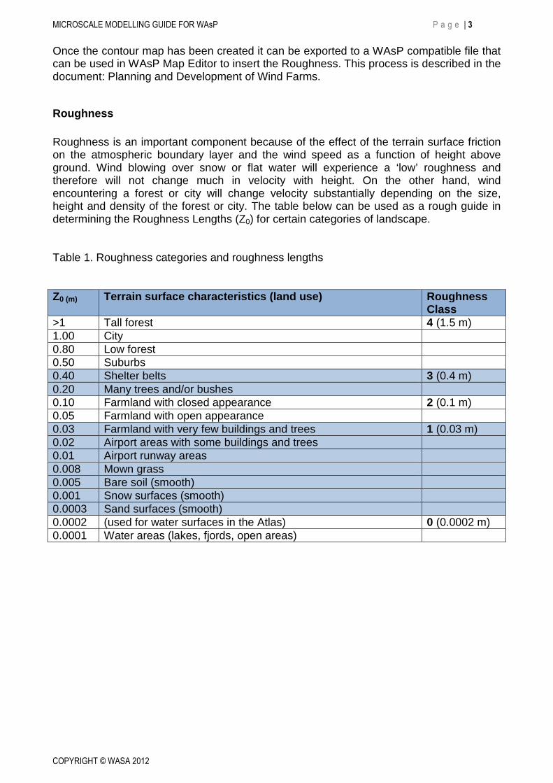
Roughness Roughness is an important component because of the effect of the terrain surface friction on the atmospheric boundary layer and the wind speed as a function of height above ground. Wind blowing over snow or flat water will experience a ‘low’ roughness and therefore will not change much in velocity with height. On the other hand, wind encountering a forest or city will change velocity substantially depending on the size, height and density of the forest or city. The table below can be used as a rough guide in determining the Roughness Lengths (Z0) for certain categories of landscape. Table 1. Roughness categories and roughness lengths Z0 (m) Terrain surface characteristics (land use) Roughness
Class >1 Tall forest 4 (1.5 m) 1.00 City 0.80 Low forest 0.50 Suburbs 0.40 Shelter belts 3 (0.4 m) 0.20 Many trees and/or bushes 0.10 Farmland with closed appearance 2 (0.1 m) 0.05 Farmland with open appearance 0.03 Farmland with very few buildings and trees 1 (0.03 m) 0.02 Airport areas with some buildings and trees 0.01 Airport runway areas 0.008 Mown grass 0.005 Bare soil (smooth) 0.001 Snow surfaces (smooth) 0.0003 Sand surfaces (smooth) 0.0002 (used for water surfaces in the Atlas) 0 (0.0002 m) 0.0001 Water areas (lakes, fjords, open areas)
2. Click on File|Open Select the vector map (contour map created earlier with the SAGA GIS software).
A pop up window might appear indicating that successive points have a resolution of less than 2 metres. These points can be removed without impacting on the quality of the map. Select Yes (default). A warning might also appear indicating that curves with missing or invalid height/roughness properties have been encountered. These need to be manually edited in Map Editor. Select OK (default).
3. To view the vector map click on Window|Map Image
5. It is necessary to load a background map so that the Roughness can be mapped. The background map can be any image of the area of interest e.g. 1:50 000 Topographical maps, 1:10 000 Orthophotos, etc. High resolution images are available from Surveys and Mapping and Department of Water Affairs and Forestry. Google Earth is a good source if no high resolution images are available The easiest is to screen capture from Google Earth using a program like Snagit.
6. The map used for demonstration purposes in this guide was captured from Google Earth. Three identifiable reference points were added (A,B and C) to make the referencing of the image in Map Editor easier. Ensure that Google Earth coordinate system is set to UTM. Make a note of the reference coordinates by right clicking on the relevant icon and selecting Properties as the coordinates will be needed when referencing the background image in Map Editor.
7. To load the background map, click on File|Load Background Map.
8. If the background map has not been referenced before, the following pop up window will appear. As no specific calibration file exists yet, click No.
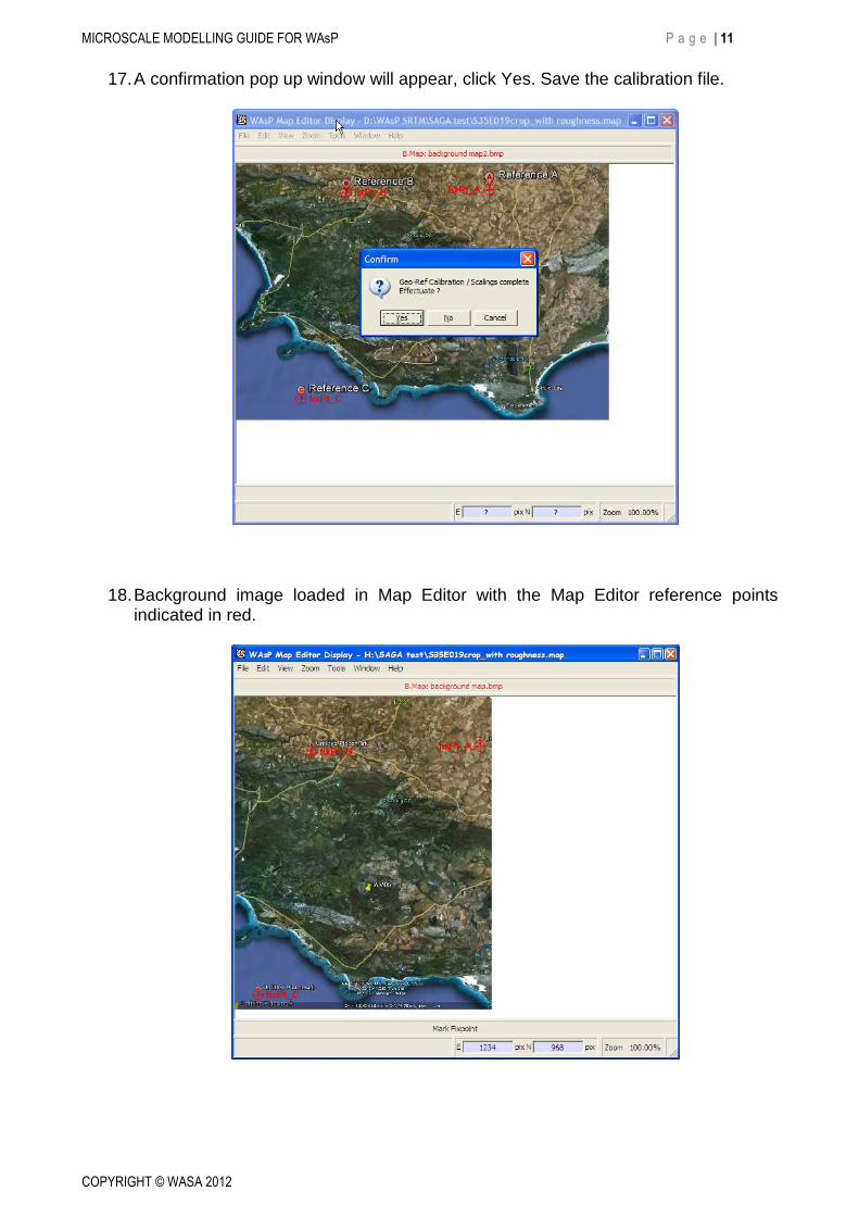
16. When the three reference coordinates have been entered click OK. The following pop up window will appear. If you are sure that the coordinates have been entered correctly (check the map extensions in the pop up window) click Yes.
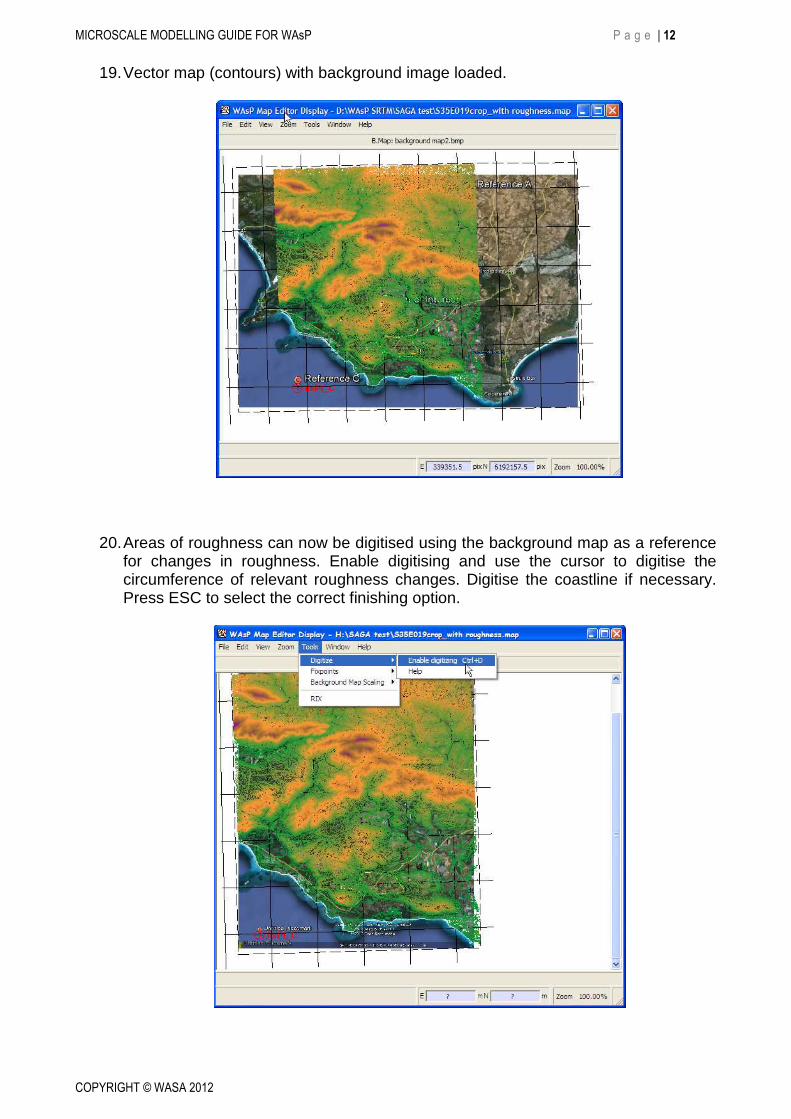
19. Vector map (contours) with background image loaded.
20. Areas of roughness can now be digitised using the background map as a reference for changes in roughness. Enable digitising and use the cursor to digitise the circumference of relevant roughness changes. Digitise the coastline if necessary. Press ESC to select the correct finishing option.
21. Using Table 1, select the appropriate roughness length (Z0). Two roughness values
need to be entered, external and internal.
22. When all the roughness areas have been digitised and appropriately classified, save the finished map as a *.map file. Your map is now ready to be imported into WAsP10.
23. Download the numerical wind atlas file closest to your point of interest from the WASA web site. Use the following URL: http://130.226.56.202/Tadpole/Viewer?gid=08aee5e5-e31f-416a-ad12-9a7a4d26f92e
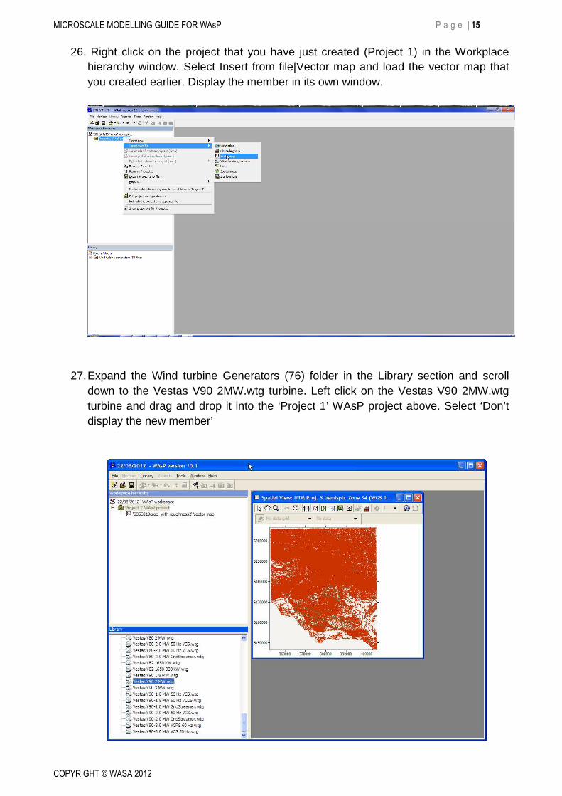
26. Right click on the project that you have just created (Project 1) in the Workplace hierarchy window. Select Insert from file|Vector map and load the vector map that you created earlier. Display the member in its own window.
27. Expand the Wind turbine Generators (76) folder in the Library section and scroll
down to the Vestas V90 2MW.wtg turbine. Left click on the Vestas V90 2MW.wtg turbine and drag and drop it into the ‘Project 1’ WAsP project above. Select ‘Don’t display the new member’
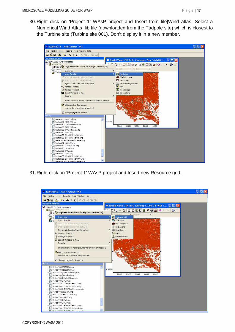
30. Right click on ‘Project 1’ WAsP project and Insert from file|Wind atlas. Select a Numerical Wind Atlas .lib file (downloaded from the Tadpole site) which is closest to the Turbine site (Turbine site 001). Don’t display it in a new member.
31. Right click on ‘Project 1’ WAsP project and Insert new|Resource grid.
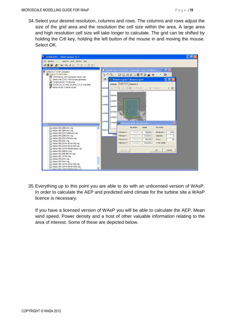
34. Select your desired resolution, columns and rows. The columns and rows adjust the size of the grid area and the resolution the cell size within the area. A large area and high resolution cell size will take longer to calculate. The grid can be shifted by holding the Crtl key, holding the left button of the mouse in and moving the mouse. Select OK.
35. Everything up to this point you are able to do with an unlicensed version of WAsP. In order to calculate the AEP and predicted wind climate for the turbine site a WAsP licence is necessary. If you have a licensed version of WAsP you will be able to calculate the AEP, Mean wind speed, Power density and a host of other valuable information relating to the area of interest. Some of these are depicted below.
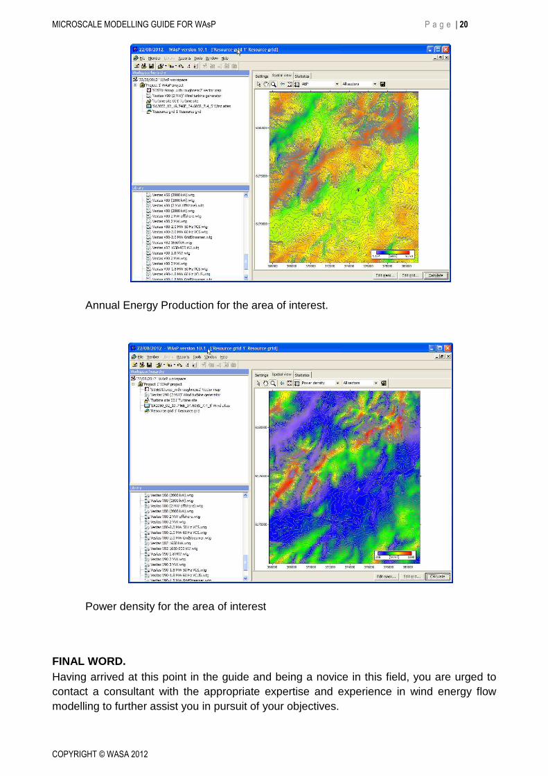
Annual Energy Production for the area of interest.
Power density for the area of interest
FINAL WORD. Having arrived at this point in the guide and being a novice in this field, you are urged to contact a consultant with the appropriate expertise and experience in wind energy flow modelling to further assist you in pursuit of your objectives.