Buckling of a stiff film

bound to a compliant substrate (part II).

A global scenario for the formation

of herringbone pattern

Basile Audoly

Institut Jean le Rond d’Alembert, UMR 7190 du CNRS,CNRS/Universite Pierre et Marie Curie, 4 place Jussieu, F-75252 Paris Cedex 05

Arezki Boudaoud

Laboratoire de Physique Statistique, UMR 8550 du CNRS/Paris 6/Paris 7Ecole normale superieure, 24 rue Lhomond, F-75231 Paris Cedex 05

Abstract

We study the buckling of a thin compressed elastic film bonded to a compliantsubstrate. We focus on a family of buckling patterns, such that the film profile isgenerated by two functions of a single variable. This family includes the unbuck-led configuration, the classical primary mode made of straight stripes, as well thepattern with undulating stripes obtained by a secondary instability investigated inthe first companion paper, and the herringbone pattern studied in last compan-ion paper. A simplified buckling model relevant for the analysis of these patternsis introduced. It is solved analytically for moderate or for large residual compres-sive stress in the film. Numerical simulations are presented, based on an efficientimplementation. Overall, the analysis provides a global picture for the formationof herringbone patterns under increasing residual stress. The film shape is shownto converge at large load to a developable shape with ridges. The wavelength ofthe pattern, selected in a first place by the primary buckling bifurcation, is frozenduring the subsequent increase of loading.

Key words: Buckling, Plates, Thermal stress, Asymptotic analysis, Energymethods

Preprint submitted to Elsevier 23 May 2008

1 Introduction

Buckling of thin plates is a classical subject in engineering mechanics. In par-ticular, the buckling of multi-layered materials has received much attentiondue to its importance in the design of sandwich panels (Allen, 1969). Thisfield has been the subject of recent work, in connection with the generation ofwrinkles in human skin or the templating and assembly of materials (see e.g.Genzer and Groenewold, 2006, for a review). Here, we consider the bucklingof a thin and stiff film bonded to a compliant substrate. In typical experi-ments, thin metallic films are deposited on an elastomer (Bowden et al., 1998;Huck et al., 2000; Yoo et al., 2002). When the system is cooled, compressiveresidual stress is induced in the film, caused by the mismatch in the thermalexpansion coefficients of the two layers. This can lead to buckling into straightwrinkles (Bowden et al., 1998), i. e. to a pattern that is invariant in one di-rection and has cylindrical symmetry. Other patterns may also appear (seee.g. Audoly and Boudaoud, 2007a). Here we focus on herringbone patterns,also called chevron or zigzag patterns, which have been observed for instanceby Huck et al. (2000); in such patterns, the crests and valleys of the wrinklesadopt characteristic zigzag shapes.

Herringbone patterns have been studied numerically. Chen and Hutchinson(2004) simulated the elementary cell of a periodic herringbone pattern, as-sumed to be a parallelogram; they investigated the dependence of energy onthe geometrical parameters of the cell. Huang et al. (2004) undertook simu-lations on a grid much larger than the wavelength; they first considered thecase of a Winkler foundation ( a foundation made of linear springs) and later(Huang et al., 2005) the case of a thick elastic foundation. They observed her-ringbones in either of the following conditions: with isotropic 1 compressivestress when the simulations is initialized with an array of ‘nascent’ herring-bones, or with anisotropic compressive stress and random initialization.

In the first companion paper (Audoly and Boudaoud, 2007a), we investigatedthe stability of the straight wrinkles (stripe pattern); we found that thesewrinkles soon become linearly unstable with respect to a pattern compris-ing undulating stripes. In the last companion paper (Audoly and Boudaoud,2007c), herringbones are recovered as a solution of the equations for plateson an elastic foundation, based on an asymptotic analysis in the limit of alarge buckling parameter. The present paper aims at bridging the gap be-tween these limits of moderate (first paper) and large buckling parameters(last paper), and shows that undulating stripes evolve smoothly towards her-ringbones under increasing load. This analysis is based on a simplified buckling

1 As in the companion papers, ‘isotropic’ stress is used as a synonym for ‘equi-biaxial’ and anisotropic’ as a synonym for biaxial but not equi-biaxial.

2

model which, as in Audoly and Boudaoud (2003), addresses the buckling in awell-chosen subspace of configurations for which analytical and numerical so-lutions can be derived. It provides a global picture of buckling into herringbonepatterns under increasing (from small to large) residual stress.

In this paper, our approach is to understand the formation of herringbones atlarge residual stress, characterized by faceted shapes with sharp folds, and theselection of wavelengths. This involves following the evolution of a particularpattern, not necessarily that with the lowest energy, under increasing loads. Wedo not include here the patterns that are unrelated to herringbones even if theycan be observed at small residual stress — this is the case for checkerboardsfor instance. They have been the subject of the first companion paper.

The present paper is organized as follows. In Section 2, we briefly recallthe formulation of the problem, given in the companion paper (Audoly andBoudaoud, 2007a). In Section 3, we introduce the simplified buckling modelwhich is analyzed in the subsequent sections. In Section 4, we give the resultsof the linear stability analysis and of the weakly post-buckled analysis basedon this approximate model, and compare with the exact results of the firstcompanion paper. In Section 5, we present comprehensive numerical simu-lations of the model, which allow one to explore moderate to large load. InSection 6, we undertake an asymptotic analysis of the limit of large load, andderive solutions which describes patterns similar to herringbone, found in thepreceding numerical analysis. In Section 7, we point out the existence of manylocal equilibria at large load and discuss the selection of the pattern observedin the experiments.

2 Formulation

We consider an thin elastic film bound to an elastic foundation. The dimen-sions of the film are infinite in its two in-plane directions. In the following,we write the elastic energy of the system per unit area in the frameworkof Hookean elasticity, that is assuming a linearly elastic response. The film isloaded with a biaxial, uniform residual stress. We focus on the case of compres-sive stress, which may make the film unstable. The film is described by theFoppl–von Karman plate equations with moderate deflections (Timoshenkoand Gere, 1961). The foundation is assumed to be an infinitely deep, linearlyelastic solid.

3

xy

zh

(E, ν)

(Es, νs)

u

vw

H = ∞

Fig. 1. Geometry of the problem and notations.

2.1 Film

We denote the E, ν and h the Young’s modulus, Poisson’s ratio and thicknessof the film, respectively. The reduced Young’s modulus is defined as E∗ =E/(1 − ν2). The loading is given in terms of the differential strain 2 ηx,ηy between film and substrate, the x and y directions being chosen as theprincipal directions of this differential strain (see Fig. 1 for the geometry andnotations). By this, we mean that the residual stress in the film is equivalentto that obtained by starting from the stress-free configurations of the filmand substrate, contracting the film by a factor ηx along the x direction andηy in the y direction, and finally binding the film to substrate. This definesthe reference configuration of the system. We are interested in the subsequentdeformation of the film and substrate in response to this loading.

We denote u(x, y), v(x, y) and w(x, y) the two components of the in-planedisplacements and the out-of-plane displacement of the center-surface of thefilm, respectively. Then, the film in-plane strain in actual configuration reads:

ǫxx = −ηx +∂u

∂x+

1

2

(

∂w

∂x

)2

, (1a)

ǫxy =1

2

(

∂u

∂y+∂v

∂x+∂w

∂x

∂w

∂y

)

, (1b)

ǫyy = −ηy +∂v

∂y+

1

2

(

∂w

∂y

)2

. (1c)

Using the classical approximations of the Foppl-von Karman plate theory,nonlinear terms involving the in-plane displacement (u, v) have been neglected.For simplicity, the film material is assumed to be isotropic. The constitutive

2 Traditionally, the loading is characterized in terms of the residual stress in the filmwhich, from equation (2), are related to the differential strain by σ0

xx = −E (ηx +ν ηy)/(1 − ν2) and σ0

yy = −E (ηy + ν ηx)/(1 − ν2).

4

equations for the film are those for plane-strain, two dimensional elasticity:

σxx =E

1 − ν2(ǫxx + ν ǫyy), (2a)

σxy =E

1 + νǫxy, (2b)

σyy =E

1 − ν2(ǫyy + ν ǫxx). (2c)

The stretching energy per unit area of the film reads

Efs =1

Lx Ly

h

2

∫

σαβ ǫαβ dx dy, (3)

while its bending energy per unit surface is given by the integral of the squaredmean curvature:

Efb =1

Lx Ly

D

2

∫

(∇2w)2 dx dy, (4)

where ∇ denotes the gradient of a function of two variables, (x, y). Accordingto plate theory, the bending modulus is

B =E h3

12 (1 − ν2). (5)

Finally, we write the total energy of the film per unit area as

Ef = Efs + Efb. (6)

2.2 Substrate

The substrate, which fills the half-space z < 0, has Young’s modulus Es andPoisson’s ratio νs. The substrate has linear elastic response. Introducing theFourier transform of the film deflection

w(kx, ky) =∫

dx dy w(x, y) exp[−i(kxx+ kyy)], (7)

the energy of substrate can be written as

Es =1

Lx Ly

∫

dkx dky E∗

s

√

k2x + k2

y w(kx, ky)w(−kx,−ky). (8)

It depends on only one parameter E∗

s , which is proportional to Es and is afunction of Poisson’s ratio νs,

E∗

s =Es (1 − νs)

(1 + νs) (3 − 4νs). (9)

5

For details, we refer to the first companion paper (Audoly and Boudaoud,2007a).

2.3 Optimization problem

The goal of the paper is to derive equilibrium solutions describing buckledstates. This involves minimizing the total energy, which is the sum of the filmand substrate energies:

Et({u, v, w}) = Es({w}) + Ef({u, v, w}). (10)

This energy has to be minimized with respect to the three components of thefilm’s displacement,

(u(x, y), v(x, y), w(x, y)),

for given values of the material parameters and differential strain (ηx, ηy).

3 A simplified model for the analysis of buckling

As explained in the introduction, the first companion paper is concerned withsmall to moderate residual stress, and the last one with large stress. In thepresent one, we discuss the case of intermediate loading. In particular, westudy the selection of the herringbone pattern and its wavelength. This ques-tion is of particular importance as we shall see that global energy minimizationdoes not provide a consistent selection mechanism. The general question weaddress here is how undulating stripe patterns evolve when the differentialstrain is progressively increased from the initial buckling threshold to muchlarger values. This progressive increase of the loading does take place in typi-cal experiments, whereby a sample obtained at high temperature cools downprogressively.

Pattern selection is difficult to approach based solely on numerical simulations(as in Huang et al., 2004, 2005) as it is impossible to vary systematically allthe parameters of the problem. Moreover, the final pattern depends largelyon the arbitrary initial condition. On the analytical side, we have exhaustedin the two companion papers all the methods that allow for exact results, byexploiting the presence of a small parameter in the limits of small or largeload. In contrast, no analytical solution for the buckling problem formulatedin Section 2 is available in the case of intermediate load. For this reason,we introduce a simplified buckling model. It is designed in such a way thatthe essential features of the original model are retained; on the other hand, issimple enough that it can be studied analytically and simulated very efficiently.

6

3.1 Motivation

To introduce our simplified model, we shall first list the various exact solutionsthat can be derived for the film shape, for different values of the residual stress.The first ones are the unbuckled solution, below the initial threshold, and thecylindrical mode (stripes) just above it:

w(x, y) = 0 (11a)

w(x, y) = A cos(k x), (11b)

where A is the amplitude of the mode and k the wavenumber. These classicalsolutions are recalled in the first companion paper. The undulating stripepattern, introduced in the same paper, is another solution valid slightly abovethe secondary threshold, which we rewrite as follows:

w(x, y) = A cos(k x) + b sin(k x) sin(k q y)

≃ A cos

[

k

(

x− b sin(k q y)

k A

)]

+ O(

b2

A

)

.(11c)

Here, b is the amplitude of the perturbation to the cylindrical model, andb≪ A slightly above threshold; q defines the aspect ratio of the pattern, thatis the ratio of the longitudinal and transverse wavenumbers.

Another analytical solution, derived in the last companion paper for largedifferential strain, is the Miura-ori pattern, defined by

w(x, y) = AS

x+ a tan θ(

12

+ S(

ya− 1

2

))

b

, (11d)

where a and b now define the dimensions of the unit cell of this periodicpattern.

We now formulate a key remark: for all the analytical solutions in equa-tions (11a–11d), the deflection w(x, y) is of the form:

w(x, y) = f(x− g(y)), (12)

for some functions f and g that depend on the profile considered (see Fig. 2).Indeed, for the unbuckled configuration, f(x) = 0 and g is arbitrary; for thestraight stripes, f(x) = A cos(kx) and g(y) = 0; for the undulating stripepattern, f(x) = A cos(kx) and g(y) = b sin(kqy)/(kA): for the Miura-ori(herringbone) pattern, f(x) = AS(x/b) and g(y) = −a tan θ (1/2 + S(y/a−1/2)).

7

a) b)

c) d) e)

xy

Fig. 2. All the patterns derived so far belong the class of quasi-1D patterns, as de-fined in equation (13a). (a) unbuckled, f(x) = 0 g(y) = 0; (b) straight stripes (cylin-drical pattern), f(x) = .7 cos x, g(y) = 0; (c) undulating stripes, f(x) = .7 cos x,g(y) = .6 sin y; (d) developable surface with curvilinear ridges f(x) = .8S(x),g(y) = .6 sin y; (e) herringbone pattern (also called Miura-ori and zigzag pattern),f(x) = .8S(x), g(y) = .7 (1/2 + S(y − 1/2)).

3.2 Kinematical constraints

Our aim is to study the transition from a flat pattern to straight or undulatingstripes at small strain, and to a herringbone (Miura-Ori) pattern at largestrain. Since all these patterns are of the particular form w(x, y) = f(x −g(y)), we propose to analyze the evolution of the pattern under increasingloading within this reduced space of configurations. In other words, we suggestto constrain the profile to be of the form w(x, y) = f(x − g(y)), even atintermediate load values. This approximation provides a workaround to theabsence of analytical solutions to the full problem. It is natural given theparticular form of the various exact solutions.

Technically, we consider the buckling problem as a minimization problemwithin a reduced space of configurations, which we call quasi-1D configu-rations. This space is defined as

Q = {w(x, y) | w(x, y) = f(x− g(y))} , (13a)

where the vertical bar stands for ‘such that’. It has already been emphasizedthat the planar, cylindrical, undulating stripes and Miura-Ori patterns allbelong to this class. Within this class, the deflection is no longer an arbitrary

8

function of two variables. Instead, it is fully specified by two functions f andg of a single variable. As a result, the Euler-Lagrange equations associatedwith the condition of energy minimum takes the form of coupled ordinary

differential equations for f and g in the quasi-1D problem, instead of partialdifferential equations in the original problem. In numeric calculations, thenumber of degrees of freedom is (2N) for a grid of size N × N , instead of(N2).

Even with the previous approximation, the Euler-Lagrange equations express-ing the condition of energy minimum are not solvable analytically becausethe in-plane displacements u(x, y) and v(x, y) are required in addition to thedeflection w(x, y). In order to avoid this difficulty, we shall further constrainthe kinematics of the film and seek solutions within the class Q ∩R, where

R = {u(x, y), v(x, y), w(x, y) | ∇ǫxx = 0 & ǫxy = 0} , (13b)

the strain being defined in terms of the displacement by equation (1). In thisclass, the film has uniform strain component ǫxx and a vanishing in-planeshear strain 3 . This approximation was successfully used for the analysis ofmultiscale, self-similar buckling patterns (Audoly and Boudaoud, 2003). It isa reasonable approximation for studying the evolution of the system underincreasing load; indeed, developable surfaces, such that ǫαβ = 0 for α andβ = x, y, belong to the class R by definition, those developable solutionsbeing the preferred solutions of the original problem at large compressivestress. Because of this, we avoid the difficulties associated with another popularbut much cruder approximation that consists in setting to zero the in-planedisplacements (see Jin and Sternberg, 2001, for a discussion of the drawbacksof such models).

We do not claim that the two approximations Q and R just proposed can bejustified rigorously. As a matter of fact, solutions of the simplified problemare not solutions of the original problem and we do not expect the simplifiedanalysis of buckling that follows to agree in full details with that based on theoriginal theory. Our assumptions are merely a set of convenient and reason-able approximations that allow for analytical calculations and fast numericalsimulations, provide good insights into the phenomena and capture the mainfeatures of transition towards herringbone patterns. This view is supported bythe analysis of Section 4, where the analyses carried out in the first compan-ion paper on the full model is repeated, with similar results, on the quasi-1Dmodel.

3 This class R treats differently the two in-plane directions x and y, as ǫyy may wellbe nonzero. The resulting model is not covariant with respect to in-plane rotations.This is not really a problem as the quasi-1D patterns Q that we consider are notisotropic anyway.

9

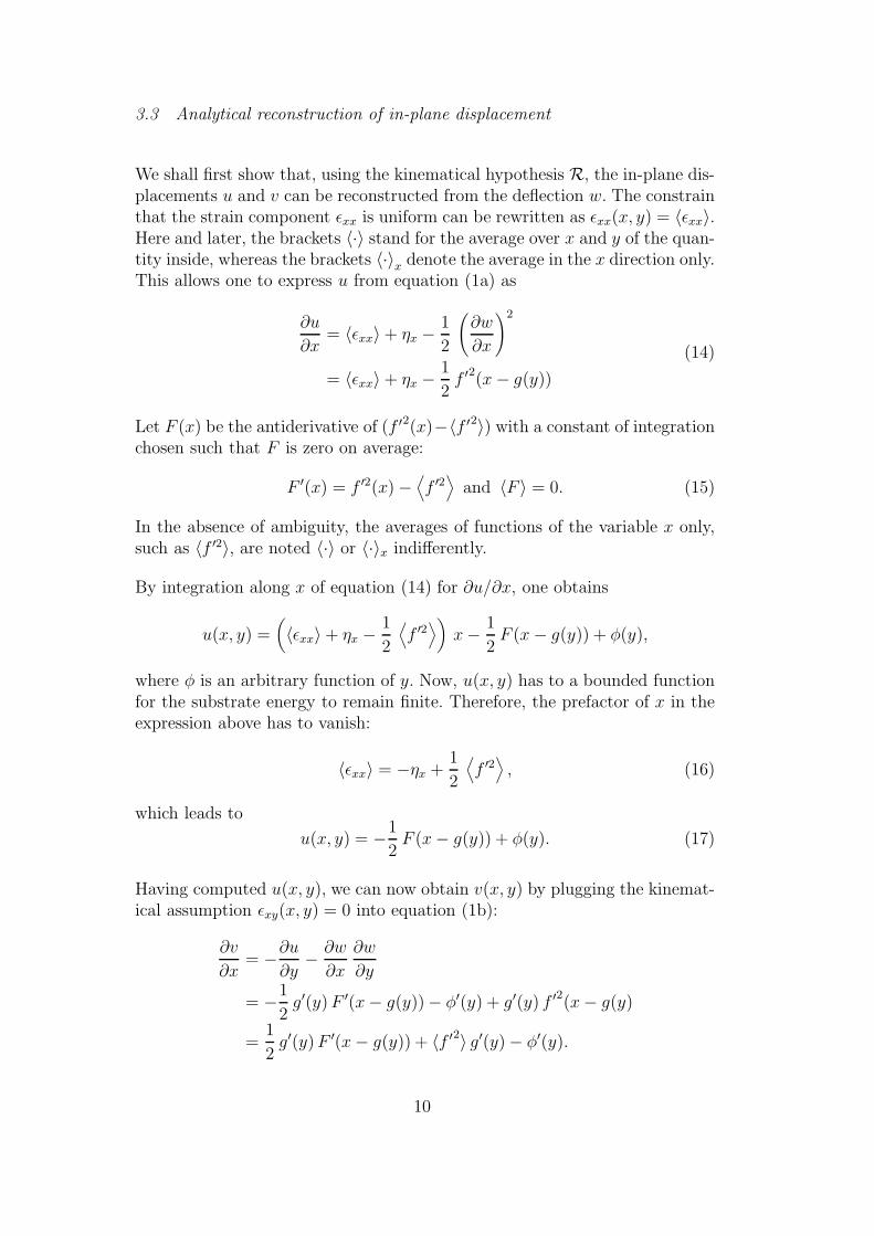
3.3 Analytical reconstruction of in-plane displacement

We shall first show that, using the kinematical hypothesis R, the in-plane dis-placements u and v can be reconstructed from the deflection w. The constrainthat the strain component ǫxx is uniform can be rewritten as ǫxx(x, y) = 〈ǫxx〉.Here and later, the brackets 〈·〉 stand for the average over x and y of the quan-tity inside, whereas the brackets 〈·〉x denote the average in the x direction only.This allows one to express u from equation (1a) as

∂u

∂x= 〈ǫxx〉 + ηx −

1

2

(

∂w

∂x

)2

= 〈ǫxx〉 + ηx −1

2f ′2(x− g(y))

(14)

Let F (x) be the antiderivative of (f ′2(x)−〈f ′2〉) with a constant of integrationchosen such that F is zero on average:

F ′(x) = f ′2(x) −⟨

f ′2⟩

and 〈F 〉 = 0. (15)

In the absence of ambiguity, the averages of functions of the variable x only,such as 〈f ′2〉, are noted 〈·〉 or 〈·〉x indifferently.

By integration along x of equation (14) for ∂u/∂x, one obtains

u(x, y) =(

〈ǫxx〉 + ηx −1

2

⟨

f ′2⟩

)

x− 1

2F (x− g(y)) + φ(y),

where φ is an arbitrary function of y. Now, u(x, y) has to a bounded functionfor the substrate energy to remain finite. Therefore, the prefactor of x in theexpression above has to vanish:

〈ǫxx〉 = −ηx +1

2

⟨

f ′2⟩

, (16)

which leads to

u(x, y) = −1

2F (x− g(y)) + φ(y). (17)

Having computed u(x, y), we can now obtain v(x, y) by plugging the kinemat-ical assumption ǫxy(x, y) = 0 into equation (1b):

∂v

∂x= −∂u

∂y− ∂w

∂x

∂w

∂y

= −1

2g′(y)F ′(x− g(y))− φ′(y) + g′(y) f ′2(x− g(y)

=1

2g′(y)F ′(x− g(y)) + 〈f ′2〉 g′(y) − φ′(y).

10

As for u, the displacement v has to be bounded and this implies that theaveraged derivative of v with respect to x is zero: 〈∂v/∂x〉x = 0. This yields,using 〈F ′〉 = 0 and 〈g′〉 = 0 (as g(y) is periodic hence bounded):

φ′(y) = 〈f ′2〉 g′(y).

We have averaged over the variable x only to obtain this equation. Pluggingback the above expression for φ′ into the expression for ∂v/∂x and carryingout the integration with respect to x, one obtains v(x, y) as

v(x, y) =1

2g′(y)F (x− g(y)) + ψ(y), (18)

where ψ is another arbitrary function, to be determined.

3.4 Energy

Having determined the displacement, we can compute the strain. The compo-nent ǫxx, which is constant by construction, has already been given in equa-tion (16). The shear component is zero by construction. The remaining com-ponent, ǫyy, can be computed from equation (1c). This yields:

ǫxx(x, y) = −ηx +

⟨

f ′2

2

⟩

(19a)

ǫxy(x, y) = 0 (19b)

ǫyy(x, y) = −ηy +1

2〈f ′2〉 g′2(y) +

1

2g′′(y)F (x− g(y)) + ψ′(y). (19c)

Anticipating the rest of the calculation, we decompose the last componentinto three contributions,

ǫyy(x, y) = ǫ(1)yy (x, y) + ǫ(2)yy (y) + ǫ(3)yy , (20)

defined by

ǫ(1)yy (x, y) = ǫyy(x, y) − 〈ǫyy(x, y)〉x (21a)

ǫ(2)yy (y) = 〈ǫyy(x, y)〉x − 〈ǫyy〉 (21b)

ǫ(3)yy = 〈ǫyy〉. (21c)

By construction, these quantities satisfy

〈ǫ(1)yy (x, y)〉x = 0 for all y, and 〈ǫ(2)yy (y)〉y = 0, (22)

11

which in particular implies 〈ǫ(1)yy (x, y)〉 = 〈ǫ(2)yy (x, y)〉 = 0. From equation (19c),one can find explicit expressions for these three terms:

ǫ(1)yy (x, y) =1

2g′′(y)F (x− g(y)) (23a)

ǫ(2)yy (y) =1

2〈f ′2〉 (g′

2(y) − 〈g′2〉) + ψ′(y) (23b)

ǫ(3)yy = −ηy +1

2〈f ′2〉 〈g′2〉. (23c)

Indeed, one can notice that 〈ψ′〉 = 0, as implied by the equality 〈∂v/∂y〉 = 0which comes itself from the fact that the displacement v(x, y) is bounded.

With the aim to formulate a minimization problem with respect to the twounknown functions f(x) and g(y) and the auxiliary function ψ(y), we computethe stretching the energy per unit area of the film, defined by equations (2a–2c)and (3) in terms of the strain tensor:

Efs({u, v, w}) =Eh

2(1 − ν2)

1

Lx Ly

∫

dx dy (ǫ2xx + ǫ2yy + 2ν ǫxxǫyy).

When the decomposition (20) for ǫyy is plugged into this expression, all thecross-products of the form (ǫ(i)yy ǫ

(j)yy ), with i 6= j vanish upon integration due

to equation (22). This leads to the following expression for the film stretchingenergy:

Efs({u, v, w}) =

Eh

2(1 − ν2)

(

〈ǫxx〉2 + 〈(ǫ(1)yy )2〉 + 〈(ǫ(2)yy )2〉 + (ǫ(3)yy )2 + 2ν 〈ǫxx〉 〈ǫyy〉)

. (24)

Here, the last term has been rewritten using the following equalities:

1

Lx Ly

∫

dx dy ǫxx ǫyy = 〈ǫxx ǫyy〉 = 〈〈ǫxx〉 ǫyy〉 = 〈ǫxx〉 〈ǫyy〉,

since ǫxx is uniform by construction.

In the stretching energy (24), the function ψ enters via a single term, namely〈(ǫ(2)yy )2〉2, whose value is given by equation (23b). Therefore, the optimalitycondition of the stretching energy with respect to this function ψ, which writesformally as

δEfs

δψ′(y)= 0,

leads toǫ(2)yy (y) = 0.

This equation allows one to determine the auxiliary function ψ,

ψ′(y) = −1

2〈f ′2〉 (g′

2(y) − 〈g′2〉).

12

We can finally write the stretching energy of the film for our reduced modelby combining the equations above:

Efs(w ∈ Q ∩R) =Eh

2 (1 − ν2)

〈g′′2〉 〈F 2〉4

+

(

〈f ′2〉2

− ηx

)2

+

(

〈f ′2〉 〈g′2〉2

− ηy

)2

+ 2ν

(

〈f ′2〉2

− ηx

) (

〈f ′2〉 〈g′2〉2

− ηy

)

, (25)

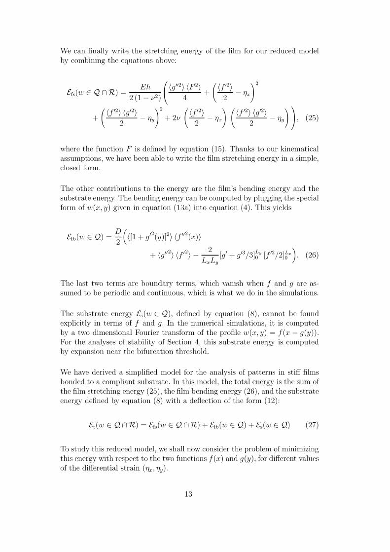
where the function F is defined by equation (15). Thanks to our kinematicalassumptions, we have been able to write the film stretching energy in a simple,closed form.

The other contributions to the energy are the film’s bending energy and thesubstrate energy. The bending energy can be computed by plugging the specialform of w(x, y) given in equation (13a) into equation (4). This yields

Efb(w ∈ Q) =D

2

(

〈[1 + g′2(y)]2〉 〈f ′′2(x)〉

+ 〈g′′2〉 〈f ′2〉 − 2

LxLy[g′ + g′3/3]

Ly

0 [f ′2/2]Lx0

)

. (26)

The last two terms are boundary terms, which vanish when f and g are as-sumed to be periodic and continuous, which is what we do in the simulations.

The substrate energy Es(w ∈ Q), defined by equation (8), cannot be foundexplicitly in terms of f and g. In the numerical simulations, it is computedby a two dimensional Fourier transform of the profile w(x, y) = f(x − g(y)).For the analyses of stability of Section 4, this substrate energy is computedby expansion near the bifurcation threshold.

We have derived a simplified model for the analysis of patterns in stiff filmsbonded to a compliant substrate. In this model, the total energy is the sum ofthe film stretching energy (25), the film bending energy (26), and the substrateenergy defined by equation (8) with a deflection of the form (12):

Et(w ∈ Q ∩R) = Efs(w ∈ Q ∩R) + Efb(w ∈ Q) + Es(w ∈ Q) (27)

To study this reduced model, we shall now consider the problem of minimizingthis energy with respect to the two functions f(x) and g(y), for different valuesof the differential strain (ηx, ηy).

13

4 Linear stability and weakly nonlinear analyses

With the aim to validate our simplified model, we repeated the weakly nonlin-ear analyses carried out in the companion paper, which are relevant for smallloading, with the aim to compare to the results of the exact model.

4.1 Primary buckling bifurcation

Let us first consider the linear stability analysis of the unbuckled state. Weuse the same rescalings as in the companion paper, and define

h∗ =h

√

12 (1 − ν2)

as a unit of length. The stiffness contrast between the two layers reads

C =E∗ h

E∗s h

∗. (28)

This large number is used to rescale the differential strain:

ηx =ηx

C−2/3, ηy =

ηy

C−2/3. (29)

For the sake of brevity, we shall not give the details of the the analysis oflinear stability, which is a classical method. The optimal film shape predictedby the simplified model from equation (27) bifurcates from planar to buckledstate above a critical differential strain. The buckled state is characterized bya harmonic profile w(x, y) with amplitude A and wavenumber k satisfying:

w(x, y) = A cos(kx)

A = 2h√

ηx + ν ηy − 3(1 − ν2)

kh∗ = C−1/3.

(30)

The planar state becomes linearly unstable when the argument of the squareroot defining the amplitude A becomes positive. As in the companion paper,the initial buckling threshold under isotropic loading is noted

ηIc = 3 (1 − ν)

Remarkably, the primary instability (30) predicted by the simplified modelis identical to that predicted by the full model (see Audoly and Boudaoud,2007a). In both cases, the buckled state involves a harmonic perturbation of

14

the film with cylindrical symmetry; the instability threshold, and the ampli-tude and wavenumbers of the unstable mode are identical. It may be surprisingthat the analysis of linear stability based on the approximate model allows oneto recover the exact results. The reason is that the simplifying kinematical as-sumptions Q and R hold both for the planar state, and for cylindrical stripepattern immediately above the primary threshold 4 .

4.2 Secondary buckling bifurcation

Having studied the initial buckling bifurcation, we can analyze the secondarybifurcations similarly. In the companion paper, this has been done based on theexact equations and we found that a secondary instability leads to undulatingstripes; this secondary instability takes place:

• strictly above the initial buckling threshold under anisotropic loading (namelywhen either ηx or ηy reaches ηI

c ),• concomitantly with the initial buckling under isotropic loading.

Here again, we shall not give the details of the analysis of linear stability ofthe stripe pattern based on the quasi-1D model. The outcome of this analysisis that straight wrinkles become linearly unstable with respect to undulat-ing stripes too. This secondary instability takes place at a threshold, denotedη′Ic in the isotropic case, which is always strictly above the initial threshold:η′Ic > ηI

c . The different predictions regarding these thresholds is apparent fromFig. 3. We conclude that the analysis of the secondary bifurcation based on thesimplified model is approximate, unlike that of the primary bifurcation. Thereason is that the solution describing undulating stripe pattern in the originalmodel does not satisfy the kinematical hypothesis R. There are fewer poten-tially unstable modes in the quasi-1D model as only those compatible withthe kinematical assumptions are available; as a result, the buckling thresholdis overestimated in the quasi-1D model. This discrepancy is in fact minor, fortwo reason: first, we qualitatively recover the same type of secondary insta-bility, leading to undulating stripes; second, the undulating stripes is actuallythe optimal shape of the quasi-1D model just above the primary bucklingthreshold ηI

c , although this is not apparent from the present linear stabilityanalysis (see end of Section 5).

4 This is not a coincidence: the main motivation for the quasi-one dimensionaldeflection, of the form (12), that is encompasses analytical solutions for the filmprofile, which includes the cylindrical pattern.

15

0 2 4 6 8 100

1

2

3

4

0 2 4 6 8 100.0

0.2

0.4

0.6

0.8

1.0(a) (b)

ηηIc

ηηIc

q b/A

η = ηIcη = ηI

c

η = η′Icη = η′Ic

Fig. 3. Linear stability analysis of the cylindrical pattern with respect to zigzags:comparison of the predictions of the approximate quasi-1D model (solid curves) withthe exact result (dotted curves) from Audoly and Boudaoud (2007a). (a) Linearlyunstable longitudinal wavenumber q (dark grey region) and most unstable wavenum-ber q (thick curve). (b) Rescaled amplitude b/A of the zigzag perturbation. Bothplots are made with Poisson’s ratio ν = 0.3.

4.3 Post-buckling analysis

These analysis of linear stability can be complemented by the nonlinear anal-ysis of post-buckled undulating stripes. The results, based on either the fullor the quasi-1D model, are compared in Fig. 3. For the sake of brevity, weomit the details of the calculations for the quasi-1D model, which are similarto those for the full model obtained by Audoly and Boudaoud (2007a).

Although the simplified model does not yield exact predictions for the sec-ondary instability threshold, it captures the most salient features of the sys-tem: the existence of a primary bifurcation leading to a stripe pattern and ofa secondary bifurcation leading to undulating stripes are captured correctly.The thresholds and amplitudes relevant for the primary bifurcations are exact,although those for the secondary bifurcations are approximate (and compa-rable to the exact ones). This validates our suggestion to use the quasi-1Dmodel as a toy model for analyzing the buckling of a stiff film bonded to acompliant substrate. This is the aim of the rest of the paper, where bucklingis investigated under intermediate to large loads.

5 Numerical simulations

The quasi-1D model is first studied numerically, at intermediate loads: weassume the differential strain to be significantly larger — but not larger byorders of magnitude — than the primary and secondary thresholds ηI

c and η′Ic .In the absence of analytical methods of solution applicable to this situation,

16

05

10

-50

5

00

05

10

101

(a) (b) (c)

xx y

yf(x) g(y)

ηη

η ηη = 6.37

2π

2π2π4π4π4π

2π

4π

Fig. 4. A typical simulation session of the quasi-1D model, for increasing values ofdimensionless load η (bold arrows). (a) Numerical solutions f(x) and (b) g(y) fordifferent values of η. (c) Visualization of the deflection w(x, y) = f(x − g(y)) for aparticular value of η = 6.37, corresponding to the thick curves f(x) and g(y) in (a)and (b). The simulation extends over (x, y) ∈ [0, Lx] × [0, Ly] with Lx = Ly = 4π,and is for isotropic load.

we resort to numerical simulations.

5.1 Implementation

The energy of the quasi-one dimensional model (27) is minimized with respectto the values of the functions f(x) and g(y) discretized on even meshes, eachhaving a number of points that is a power of 2, in the range 64–256. Thestretching and bending energy of the film, given by equations (25) and (26),are computed using finite differences. The energy of the substrate (8) is com-puted using a Fast Fourier transform algorithm (FFT). The energy is thenminimized by the method of conjugate gradient descent. The size Lx × Ly ofthe squared simulation cell is chosen at the beginning of the simulation. Usingperiodic boundary conditions, we effectively simulate an infinite array of suchelementary cells. Ideally, our simulation cell is much larger than the expectedsize of the buckling pattern, which is of order 2π in dimensionless units (recallthat the wavenumber of the primary instability is 1 in dimensionless units);in some cases, especially when using a fine spatial discretization, the actualdimensions of the simulation cell had to be lowered to values comparable towavelength of the buckling pattern in order to keep the simulation time rea-sonable. We used rescaled quantities in all the numerical simulations, therebyavoiding to introduce unnecessary errors caused by machine accuracy.

In our simulations, we focused on the case of isotropic differential strain,η = ηx = ηy. Then, the only control parameter in the simulation is therescaled differential strain, η. The result of a typical simulation session isshown in Fig. 4. The functions f and g are initialized with very small, ran-dom values. Starting from η = 0, we progressively increase the differentialstrain, and observe the profiles of the numerical minimizers f(x) and g(y). Asexplained earlier, the kinematical assumptions in the model allow for offline,

17

symbolic calculations of the in-plane displacement. The calculations that re-main to be done online are essentially the calculation of integrals involving f , g,their derivatives and powers, which is effectively a one-dimensional problem 5 ,and can be done very quickly, at an interactive rate on a standard personalcomputer. This makes it quite easy to track solutions under increasing or de-creasing loading, and to discriminate between continuous and discontinuousbifurcations, as reported in the end of the present Section.

5.2 Results

In the simulation shown in Fig. 4, we first observe the unbuckled state for lowdifferential strain: f(x) ≈ 0 for all x and g(y) ≈ 0 for all y. When η is increasedabove a primary threshold, the function f starts to make undulations, althoughthe profile g(y) remains flat. This corresponds to the stripe pattern. At asecondary threshold, the function g starts to make undulations, producingundulating stripes. The values of the thresholds, amplitudes and wavelengthare studied in details next, see Fig. 5. They are consistent with the analyticalpredictions of Section 4. When the loading is further increased, the function fchanges progressively from a sinusoidal to a non-smooth, sawtooth-like shape.

In Fig. 5, we present a more detailed analysis of the simulation results, forν = 0.3. When the loading is increased, starting from η = 0, the unbuckledpattern, characterized by 〈f ′2〉 = 0 and 〈g′2〉 = 0 is first observed. At athreshold very close to that predicted by the theory, η = ηI

c = 3 (1− ν) = 2.1,the function f(x) bifurcates. This corresponds to the emergence of a stripepattern, set inset (B), with a wavelength, 2π in rescaled units, consistent withthat predicted by the linear stability analysis. The squared amplitude of thepattern, 〈f ′2〉, is found to vary linearly with the distance to threshold η − ηI

c ;this is characteristic of a supercritical (continuous) bifurcation. This is all inagreement with the results of the previous section and with those of the exactmodel given in the first companion paper (Audoly and Boudaoud, 2007a).

The stripe pattern persists until a secondary threshold is reached. This thresh-old is very close to the threshold, η′Ic (ν = .3) = 5.88, predicted by linearstability analysis of the straight wrinkles, see Section 4. This secondary bi-furcation turns out to be subcritical (discontinuous): both the energy and thenumber 〈g′2〉 change by a finite amount in a single simulation step. Above

5 At every step in the minimization, we need to reconstruct the 2D profile of theplate using equation (12) before we can carry out the fast Fourier transform nu-merically. This is the only operation that is two-dimensional, i. e. that involves N2

operations where N is the number of discretization points). Being based on a highlyoptimized algorithm, the fast Fourier transform, it remains very quick and did notslow noticeably the calculation down.

18

0 2 4 6 8 10

0.1

0.2

0.3

0.4

0.5

0.6

0

5

10

15

20

2 4 6 8 10

3.0

3.5

4.0

4.5

〈f ′2〉

〈g′2〉

〈f ′2〉

〈g′2〉

Et

η3/4

η

η

f(x)

g(y)

(A)

(B)

(C)

(D)

(A) (B)

(C)

(D)η = 1.82η = 1.82

η = 5.01 (↑)

η = 8.19

η = 5.01 (↓)η = 5.01 (↓)

η=η

I c

η=η

I c′

x

x

x

x

y

y

y

y

2π

2π

2π

2π

2π

2π

2π

2π

4π

4π

4π

4π

4π

4π

4π

4π

2π

2π

2π

2π

4π

4π

4π

4π

−4

−4

−4

−4

4

4

4

4

Fig. 5. Simulations based on the quasi-1D model. In the upper-left part of thediagram, the quantities 〈f ′2〉 and 〈g′2〉 are given as a function of the control param-eter η, which is first increased and then decreased. Two bifurcations, involving ffirst and then g, take place very close to the theoretical thresholds (vertical dottedlines). A hysteresis curve is followed when the loading is first increased and thendecreased. In the lower left diagram, the energy of the solution is plotted. On theright-hand sides, the 3D configurations of a few representative configurations areshown. The rectangular simulation cell has dimensions Lx = Ly = 4π and resolutionNx = Ny = 32. Poisson’s coefficient is ν = 0.3.

the secondary threshold, undulating stripes are obtained; the evolution of thispattern when the loading is further increased is analyzed in the next section.

When the loading is subsequently decreased, the solution follows a hysteresiscycle. Below η′Ic (but above ηI

c), the film pattern is still given by undulatingstripes, although it was made of straight stripes during the loading stagein the same range of differential strain. The energy profile at the bottom ofFig. 5 reveals that the undulating pattern has a lower energy than the straightstripes. In retrospect, it appears that the system has remained trapped in alocal minimum of energy in the range ηI

c < η < η′Ic and under increasingloading, which it could not escape until this local energy minimum becamelinearly unstable, at η′Ic .

19

These numerical results are in complete agreement with the analysis of thesimplified model presented in the previous section. Furthermore, the numericalobservation of a hysteresis cycle mitigates the main discrepancy found betweenthe exact model and the simplified one. Recall that, with the exact modelunder isotropic isotropic loading, straight stripes become linearly unstableimmediately above the initial buckling threshold ηI

c , although in the quasi-1Dmodel they were found to remain linearly stable over a range ηI

c < η < η′Icwhich extends much beyond the initial buckling threshold. As revealed bythe numerics, undulating stripe patterns are actually present in the quasi-1Dmodel immediately above the initial threshold too, and are indeed the stateof lowest energy — however, they are not accessible by the analysis of linearstability as they appear by a discontinuous bifurcation.

6 Analytical and numerical solution in the limit of large load

Numerical simulations have confirmed the emergence of an undulating patternby a sequence of two bifurcations, namely an initial bifurcation towards acylindrical pattern and a secondary bifurcation leading to undulations. In thepresent section, we investigate how this pattern evolves when residual stress isfurther increased. We show in details how the pattern, emerging in a first placeas a small amplitude perturbation on top of the straight stripe pattern, evolvesprogressively towards a developable shape with crests and valleys comprisingangular points. We shall also address the selection of the wavelengths of thepattern obtained at large differential strain, a question which has remainedunsettled so far.

6.1 Penalization of the stretching energy

We shall show that the quasi-1D model can be solved analytically in limitof large differential strain, ηx ≫ 1 and ηy ≫ 1. As explained before, thismodel is based on approximations but is expected to provide good insightsinto the behavior of the full model — in the last companion paper, we discussin detail the similarities and differences of the predictions of the two modelsfor large load. Note that, by large differential strain, we mean large rescaled

differential strain ηα = ηα/C−2/3 ≫ 1. The stiffness contrast C is a large

number by assumption and so the rescaled strain can be large although thephysical strain remains small; in fact, this happens when

1 ≪ ηα ≪ C2/3. (31)

In this regime, it is consistent to use the assumption of a linear elastic responsefor the substrate and the Foppl-von Karman equations for the film. In the rest

20

10 20 50 100 200 5000.1

1

10

100

1000

10 20 50 100 200 500 103103 2.1031

10

100

1000

104〈f ′2〉2 η

〈g′2〉1

Et

〈f ′′2〉 1

43

ηη

(a) (b)

Fig. 6. Numerical confirmation of the scaling laws for 〈f ′2〉, 〈g′2〉, 〈f ′′2〉, and Et atlarge η. Simulation parameters are Lx = Ly = 2π, Nx = 64, Ny = 32 and ν = 0.3,with isotropic differential strain.

of this section, we consider this range of loading, defined by equation (31): wederive the features of the energy minimizers analytically and compare withnumerical simulations.

A classical result of plate theory is that the stretching energy, associated witha stiffness E h directly proportional to the small parameter h, becomes dom-inant over the bending energy whose stiffness E h3 scales like the third powerof h. As a result, thin plates subjected to significant load attempt to minimizetheir stretching energy in a first place (mathematically, this defines a penal-ization problem). Unless this is prevented by the boundary conditions or bythe geometry, their center-surface adopts a profile close to a developable sur-face — this happens for instance in folds and d-cones analyzed by Lobkovsky(1996); Ben Amar and Pomeau (1997). Therefore, we expect the optimal filmshapes to make the film stretching energy (25) vanish at dominant order:

Efs(w ∈ Q ∩R) =Eh

2 (1 − ν2)

〈g′′2〉 〈F 2〉4

+

(

〈f ′2〉2

− ηx

)2

+

(

〈f ′2〉 〈g′2〉2

− ηy

)2

+ 2ν

(

〈f ′2〉2

− ηx

) (

〈f ′2〉 〈g′2〉2

− ηy

)

.

The same argument will be used in the last companion paper where we studya family of developable patterns. For large differential strain ηx and ηy, thereare two types of factors that become formally large in this expression, namely(〈f ′2〉/2−ηx)

2 and (〈f ′2〉 〈g′2〉/2−ηy)2. We conjecture that the functions f(x)

and g(y) with lowest energy make these terms cancel:

〈f ′2〉 ≈ 2 ηx, 〈g′2〉 ≈ ηy

ηx

, (32)

as this the best way to lower the energy of the system. The prediction (32) isconfirmed by the numerical simulations shown in Fig. 6. In these simulations,the differential strain is isotropic, ηx = ηy and so 〈g′2〉 is expected to convergeto 1 for large ηx = ηy.

21

32

1 12

12

1 32

12

12

- --

-

t

S(t)

Fig. 7. Sawtooth function, as defined by equation (34).

6.2 Optimal film profile

We are left with one single term in the stretching energy, proportional to〈F 2〉. The function F has been defined in equation (15) as the antiderivativeof f ′2 − 〈f ′2〉. In order to minimize 〈F 2〉, the function f should be such thatf ′2(x) ≈ 〈f ′2〉 almost everywhere. Combining with equation (32), this yields

f ′2(x) ≈ 2 ηx for almost all x.

The solutions for this equation are sawtooth functions, with slope ±√2 ηx.

One possibility is that the sign of f ′ change periodically, as happens with thefollowing function:

f(x) → (2 ηx)1/2 ℓx S

(

x

ℓx

)

, (33)

where ℓx is half the wavelength, a free parameter of the solution. In thisequation, we have introduced the sawtooth function with period 2,

S(t) =

−1 − t if −1 ≤ t ≤ −1/2,

t if −1/2 ≤ t ≤ 1/2,

1 − t, if 1/2 ≤ t ≤ 1,

(34)

extended by periodicity for all t by S(t+ 2) = S(t)

This function is plotted in Fig. 7.

Equation (33) is not the only possibility for f(x) as one can replace S byan irregular function S such that |S ′(u)| = 1 almost everywhere. Irregularsawtooth functions are likely to be less favorable as their bending energy isunevenly distributed across the film area, but they may well lead to metastableenergy minima. The convergence of f(x) towards the profile predicted by equa-tion (33) has been observed in the simulations, see Fig. 8, left, with appropriateinitial data 6 . We shall limit ourselves to formal arguments, without attempt-

6 f(x) converges to the regular sawtooth S(x) when the load is gradually increasedpast the secondary threshold η′Ic , following the procedure discussed in Section 7.If the simulation is started with a arbitrary value of the differential strain, f(x)converges to an irregular sawtooth S.

22

2

1

1

2 50

50

1.5

1.0

0.5

0.5

1.0

f(x)

π 2πx

ππ 4π4πx y

f(x)

η1/2 g(y)η = 36.η = 73.η = 136.η = 273.η = 546.η = 1638.theory

Fig. 8. Numerical confirmation of the convergence of the functions f(x) and g(y) tothe profiles given by equations (33-35) for large η. The parameters of the simulationare the same as in Fig. 6.

ing to establish the convergence by rigorous arguments.

In order to derive the function g(y) in this limit of large applied loading, weshall first assume that 〈F 2〉 converges to a nonzero value, a hypothesis that willbe checked to be consistent at the end. The optimization problem for g is thatthe remaining term in the stretching energy, namely 〈g′′2〉〈F 2〉, is minimumunder the constraint 〈g′2〉 = ηy/ηx coming from equation (32). Technically, thisconstrained minimization problem can be solved using a Lagrange multiplierµ, and we seek the minimum of the functional

∫

g′′2dy − µ∫

g′2dy.

The corresponding Euler-Lagrange condition is the differential equation g′′′′(y)+µg′′(y) = 0; its bounded solutions are harmonic 7 functions, up to an additiveconstant that is unimportant as it corresponds to a translation of the patternalong the x axis. For a similar reason, we fix the phase of the function g(y)arbitrarily, as it corresponds to a translation of the pattern along the y axis.This yields, in the limit of large differential strain:

g(y) →(

2ηy

ηx

)1/2

ℓy sin

(

y

ℓy

)

. (35)

Here, ℓy is the typical lengthscale for g, which is another free parameter ofthe solution. The convergence of g(y) towards the profile predicted by equa-tion (35) is again confirmed by numerical simulations, see Fig. 8, right.

At large differential strain, the minimizers of our simplified model are givenby a sinusoidal function f(x) and a sawtooth function g(y), see equations (33)and (35). From equation (12), the function f determines the profile of the filmwhen cut along a vertical plane perpendicular to the average direction of theridges, although the graph of g(y) yields the shape of the crest and valleys

7 For negative µ, we also have solutions in the form of hyperbolic sine and cosinefunctions but the latter are not bounded and so are discarded.

23

of the pattern. Therefore, the optimal pattern at large load in the quasi-1Dmodel is a developable surface obtained by folding a cylindrical shape alongsinusoidal ridges, similar to that shown in Fig. 2d.

6.3 Energy of the minimizers, width of the ridges

This argument can be pushed further: by studying in more detail what happensnear the angular points for f(x), we shall be able to estimate the energy of theminimizers at large differential strain. The sawtooth profile (33) for f(x) isunphysical near the angular points, where the bending energy diverges. Thereis a small layer near these angular points where bending has to be taken intoaccount. This results in a profile that is regularized over a typical length δmuch smaller than ℓx. This length δ is similar to the width of circular ridgestudied by Pogorelov (1988). We shall estimate the ridge width δ along withthe total energy of the film for the problem at hand.

In the layer obtained by regularizing the angular points, which we call theridge, the order of magnitude of f ′ is, like everywhere, ηx

1/2. The secondderivative f ′′ is zero far from the ridges where f has a linear dependence onx; across a ridge, f ′ changes sign, and so varies by an amount comparable toηx

1/2 over a length δ. This yields the estimate f ′′ ∼ ηx1/2/δ in the ridge region.

As f ′′ is nonzero over a fraction δ/ℓx of the x axis, the average of its square isestimated as

〈f ′′2 〉 ∼(

ηx1/2

δ

)2δ

ℓx∼ ηx

δ ℓx. (36)

From this equation, we find that the bending energy (26) is of order:

Efb ∼ D 〈f ′′2 〉 ∼ D η

δ ℓx. (37)

For simplicity, we assume from now on that the differential strain is notseverely anisotropic, i. e. that ηx and ηy have the same order of magnitude,called η: we write η ∼ ηx ∼ ηy.

Let us come back to the remaining term in the stretching energy (26), whichis proportional to 〈g′′2〉〈F 2〉. The factor 〈g′′2〉 can be estimated easily, as equa-tion (32) implies that g′ is a quantity of order 1. As a result, g′′ is comparableto 1/ℓy, where ℓy is the typical length over which the smooth function g(y)varies, and 〈g′′2〉 ∼ ℓy

−2. In order to estimate the other factor, 〈F 2〉, we notethat F is defined as the antiderivative of f ′2 − 〈f ′2〉, a quantity which is zeroeverywhere, except in the ridge regions, of length δ, where it is comparable toη. This yields

F ∼ δ η.

24

Combining these results, we estimate the first term in the stretching energyas

〈g′′2〉 〈F 2〉 ∼ δ2 η2

ℓy2 (38)

Note in passing that we can validate the initial and main assumption of ourreasoning: if equation (32) were not satisfied, the stretching energy would be oforder Ehη2; when it is satisfied, it is of order Ehη2 (δ/ℓy)

2 by the calculationabove. Anticipating on the fact that δ ≪ ℓy, something that we shall check inthe end, we confirm the fact that the constraints (32) allow a drastic decreasein the stretching energy, by a factor (δ/ℓy)

2.

We have just shown that the stretching energy of the film is comparable to

Es ∼ Eh〈g′′2〉 〈F 2〉 ∼ Ehδ2 η2

ℓy2 . (39)

The ridge width δ results from a balance of two antagonistic effects. Thestretching energy above is lower when δ is smaller, although the bending en-ergy (37) is lower when δ is larger. Balancing these two terms, we obtain anestimate for this width:

δ

ℓy∼(

h2

ℓxℓyη

)1/3

. (40)

Noting λ = 2π/k = 2π h∗C1/3 the wavelength of the initial, cylindrical buck-ling pattern, and rescaling the in-plane lengths ℓx and ℓy using λ, we have

ℓx =ℓxλ

∼ ℓxhC1/3

, ℓy =ℓyλ

∼ ℓyhC1/3

. (41)

Recalling the definition (29) of the rescaled differential strain, we rewrite theestimate for δ given above in equation (40) in terms of dimensionless quanti-ties:

δ

ℓy∼ 1(

ℓx ℓy η)1/3

. (42)

This expression confirms that the ridge width is small compared to the wave-length ℓy in the strongly nonlinear limit, η ≫ 1, assuming that the wavelengthsof the pattern are comparable to the wavelength λ of the stripe pattern at theonset of bifurcation threshold (ℓx,y ∼ λ implies ℓx,y ∼ 1). This makes ourapproach consistent.

With the ridge width given in equation (42), the stretching energy (39) andbending energy of the film are both of the same order of magnitude, and thetotal energy of the film reads

Ef ∼ Eh

(

h2

ℓxℓy

)2/3

η4/3 = Ehη4/3

C4/3 (ℓx ℓy)2/3. (43)

25

We shall now show that the energy of the substrate is negligible, that is muchsmaller than Ef in this limit. The typical deflection w is found from equa-tion (33) as w ∼ f ∼ η1/2 ℓx, whereas the wavevector k that brings the domi-nant contribution to the substrate energy is 1/min(ℓx, ℓy). Plugging this intothe definition (8) of the substrate energy yields

Es ∼ Es ηℓx

2

min(ℓx, ℓy).

The ratio of this substrate energy to the film energy (43) reads

Es

Ef∼

ℓx8/3

ℓy2/3

min(ℓx, ℓy)

1

η1/3. (44)

Whenever the right-hand side in equation (44) is small, the energy of thesubstrate is negligible, |Es| ≪ |Ef |, and the total energy is estimated as:

Et ∼ Ef ∼ Ehη4/3

C4/3 (ℓx ℓy)2/3, provided

ℓx8/3

ℓy2/3

min(ℓx, ℓy)≪ η1/3. (45)

This happens in particular in the limit of large load, η ≫ 1, when the patternwavelengths are comparable to the buckling wavelength λ at the onset ofbifurcation — then, ℓx and ℓy are of order unity.

The main result of this scaling analysis of the ridge is that the total energyof the pattern goes like η4/3 at large differential strain, when all the other pa-rameters remain unchanged, see equation (45). We have confirmed this scalingbehavior with the numerical simulations shown in Fig. 6, right. In this figure,the numerical value of 〈f ′′2〉 at large η is also compared to a prediction thatcan be made by combining equations (36) and (40), namely 〈f ′′2〉 ∼ η4/3, anda good agreement is found.

6.4 Tentative prediction of wavelengths based on energy minimization

It is interesting to optimize the energy (45) of the pattern with respect toits wavelengths, ℓx and ℓy. The result is somewhat surprising as we shall nowshow that the optimal rescaled wavelengths are ℓx → 0 and ℓy → ∞. Indeed,let us introduce a large number, ρ, which will soon be identified with theaspect ratio ℓy/ℓx ≫ 1 of the pattern, and consider wavelengths that scalelike ℓy ∼ (η)1/7 ργ and ℓx ∼ (η)1/7/ρ1−γ , where γ is a number in the rangeγ ∈ [1

2, 5

7]. By plugging these expressions into equation (45), we find that the

energy scales like Et ∼ E hC−4/3 η24/21/ρ43 (γ− 1

2) and therefore goes to zero

26

at fixed η when ρ → ∞, given that γ > 12. The condition on the right-

hand side of equation (45) is satisfied provided 1/ρ5−7 γ

3 → 0, and this isindeed the case with γ < 5

7. We have shown that the pattern that achieves

the absolute minimum of energy is made of curvilinear ridges with ℓx ≪ ℓy:the spacing between ridges is much smaller than than the wavelength of thesesinusoidal ridges. A similar oddity will be obtained with the full model (Audolyand Boudaoud, 2007c). In contrast, the two wavelengths of the pattern arecomparable in the experiments. This points to the fact that the wavelengthsof the pattern are not selected by energy minimization at large load but insteadby a trapping mechanism, as explained in Section 7.

6.5 On the shape of crests and valleys

At large load, we have found that the quasi-1D model predicts a developablepattern made of piecewise cylindrical shapes connected by sinusoidal ridges, asin Fig. 2d. In the last companion paper, we shall show that the exact modelpredicts a similar pattern in this limit, but with zigzag crests and valleyscomprising angular points. This discrepancy concerning the shape of crestsand valleys is caused by the kinematical assumptions at the basis of the quasi-1D model, as discussed in detail in the forthcoming paper. Although it does notpredict the correct ridge shapes, the quasi-1D model shows how undulatingpatterns, obtained by a sequence of two buckling bifurcation, progressivelyevolve towards a piecewise developable shape. Even more importantly, thisapproximate models explains how the wavelengths of the pattern are selected,as investigated in the next Section.

7 Selection of wavelength, metastability and trapping

In our simulations of the quasi-one dimensional model, the differential strainis progressively increased from zero. As explained in Section 5, we observe abifurcation to a straight stripe pattern which becomes unstable towards anundulating zigzag pattern — sometimes, the stripe pattern is not observed atall as the system jumps directly to the zigzag pattern, see Fig. 5. When thedifferential strain is further increased, the smooth undulating pattern evolvesprogressively into a pattern with sharp curvilinear ridges, as shown in theprevious Section. When the loading is increased by small increments and thesystem is allowed to relax at each step, this smooth transition from undulatingstripes to a developable pattern with ridges does not involve any noticeablechange in the wavelengths of the pattern (this concerns both the wavelengthalong the average ridge direction and the spacing between neighboring ridges).As a result, the piecewise developable patterns obtained at the maximum

27

loading that the simulation can handle, typically η ∼ 103, have wavelengthsclose to λ = 2π/k, the wavelength of the cylindrical pattern at the onset ofbuckling.

In contrast, we argued in Section 6.4 that the pattern with lowest energy isa piecewise developable shape having widely different longitudinal and trans-verse wavelengths: its inter-crest spacing is much smaller than λ, although thewavelength of the crests (and valleys) is much larger than λ. This points tothe fact that the system has many local equilibrium configurations and that itis unable to pick that with lowest energy in the simulation. In the presence ofa small amount of dissipation, or when the dimension of the film is large butfinite, the wavelength of a pattern cannot not vary smoothly but by jumps,by a local doubling of wavelength for instance. As a result, the system is ableto explore a limited set of wavelengths only. Consequently, the wavelength isfrozen during loading, and remains comparable to its value λ at the onset ofbuckling. We claim that the wavelengths observed at relatively large bucklingnumber in the experiments result from this trapping mechanism, and not froma principle of energy minimization.

In the present section, we provide numerical evidence of this trapping mech-anism and show that a pattern keeps its wavelengths and overall geometryunchanged (unless severely perturbed) even though they are no longer theones with lowest energy. The simulations presented in this section are carriedout on a domain several times larger than the initial wavelength of the in-stability, and so the unit simulation cell comprises many wavelengths of thepattern.

In Fig. 9, we illustrate the existence of several local equilibria by showing twonumerical equilibria observed in the same loading conditions but followingdifferent loading histories. In the upper part of the figure, the pattern has beenobtained with a slowly increasing loading and the resulting pattern is periodic.In the lower part of the figure, it has been obtained with a non-monotonicloading varied by jumps; the resulting pattern is not periodic along the ydirection. The two patterns correspond to the same set of final parameters.There are five wavelengths across the width of the unit cell in the first case,and seven in the second case. This illustrates the dependence of the patternon the loading history, and the existence of many local equilibria.

This trapping mechanism is clearly demonstrated by the simulations shown inFig. 10. The simulation is started with a differential strain η a few times abovethe primary threshold, typically η ≈ 5. Differential strain is then increasedsmoothly. As explained earlier, the herringbone pattern obtained in this wayhas periodic crests (or valleys) with a wavelength close to the initial bucklingwavelength λ. The spacing between these crests and valleys is of the sameorder of magnitude. When η is further increased, the geometry of the pattern

28

2 4 6 8 10

4

2

2

4

2 4 6 8 10

3

2

1

1

2

3

4

(a)

(b)

f(x)g(x)

Fig. 9. Existence of multiple equilibria with identical parameters and loading. Forboth simulations, the parameters are Nx = Ny = 128, ℓx = ℓy = 10π, ν = .3 andη = 6.36 (a) Et = −31.9 (b) Et = −23.1. Note the difference in wavelengths.

10 20 50 100 200 50010000.00.51.01.52.02.53.03.5

2π

2π

2π

2π

4π

4π

4π

4π

2π

2π

2π

2π

4π

4π

4π

4π

6π

6π

6π

6π

8π

8π

8π

8π

x

x

x

x

y

y

y

y

Et

η4/3

η

ℓy = 2π

ℓy = 2π

ℓy = 8π

ℓy = 8π

Fig. 10. Tracking of numerical solutions for a loading cycle. The system is ‘shaken’at the maximum loading to allow better relaxation of the energy, and jumps toa pattern with large wavelengths. The energy is plotted along this loading cycle,revealing a hysteresis: under increasing loading, the numerical solution is trapped ina local minimum of energy. Simulation parameters are Lx = 4π, Ly = 8π, Nx = 32,Ny = 64, ν = .3

29

ηηIc η′c

I

(P) (C) (U) (D)

Fig. 11. Summary of patterns under increasing load η. (P) flat, unbuckled state,(C) straight wrinkles (cylindrical state), (U) undulating stripes, (D) Developablepattern. The transitions from P to C and from P to U correspond to the primaryand secondary buckling at well-defined thresholds in compressive strain, whereas theevolution from U to D is smooth. Pattern D has curvilinear ridges in the quasi-1Dmodel (see Section 6) but piecewise straight zigzag ridges in the full model (seeanalysis of the Miura-ori pattern in the last companion paper).

changes very little, and none of the wavelengths varies noticeably (see insets ontop of Fig. 10); the only difference is that the pattern has a higher and highercontrast as the deflection of the film increases. However, if the simulation isreset to an almost flat configuration at large strain η, of the order of 1000, theinter-crest spacing and longitudinal wavelength jump to the largest accessiblevalue, i.e. to the size of the simulation cell Lx and Ly. This is consistentwith the fact that the energy (45) decreases when the wavelengths ℓx or ℓyincrease 8 . When the loading η is decreased from there, down to values assmall as η ∼ 5, the wavelengths do not change either. We have computed theenergy along these two branches and found that the second pattern always hasa significantly lower energy that the first one. This means that the solutionobtained under increasing loading has remained trapped in a local equilibriumconfiguration all the way up to the maximum applied loading, η ∼ 103.

The numerical observations in Fig. 10 confirm the findings of Section 6.3,namely that the optimal wavelengths are widely different from the wavelengthλ at the onset of buckling. When the residual stress is gradually increased, thepattern is not selected by global energy minimization: the transverse and lon-gitudinal wavelengths of a herringbone pattern remain locked in a metastableminimum under increasing load. In the experiments, they are probably fixedby the initial and secondary buckling bifurcations, leading to undulating pat-terns.

30

8 Conclusion

In this paper, we investigated the formation of herringbone patterns in com-pressed thin films bonded to a compliant substrate, based on a simplifiedbuckling model. This model is built by imposing kinematical constraints onthe film shape. These kinematical constraints were chosen so as to be compat-ible with analytical solutions of the problem available in the limits of smalland large loads — the patterns such as the checkerboard that are unrelatedto the formation of herringbones, are not included in the present analysis.This reduced model has the remarkable property that its stretching energyvanishes whenever the actual stretching energy vanishes; as a result, smoothdevelopable surfaces are favored in the limit of large compression, as in theexact model. A validation is provided by comparison of the results of a linearstability analysis and of a weakly nonlinear analysis, based either on the sim-plified or exact models. A similar buckling model has been used to analyzemultiscale, self-similar buckling patterns in thin elastic plates (Audoly andBoudaoud, 2003), and might be applicable to other buckling problems.

Using numerical simulations of the simplified model, we recovered the initialand secondary buckling bifurcations, first to a cylindrical pattern and secondto an undulating pattern. The undulating pattern evolves smoothly towardsa developable pattern with ridges at large differential strain. This developablepattern is very similar to the Miura-ori pattern analyzed in the last companionpaper, and to the experimental herringbone patterns; a minor difference, com-ing from the approximations introduced, is that the numerical minimizers havecurved — and not sawtooth-like — crests and valleys in the quasi-1D model.By the developability condition, the ratio of principal residual stresses can beextracted from the profile g(y) of the crests and valleys; see equation (32).

Our numerical simulations reveal that many equilibrium states are possi-ble. When the compressive strain is gradually increased, the system remainstrapped in a local minimum of energy which is not the global one. As a result,the longitudinal and transverse wavelengths of herringbone patterns in realexperiments are expected to be comparable to the buckling wavelength λ atthreshold; the precise value of its aspect ratio depends on the detailed historyof loading at the early stage of the experiment.

Our results are in qualitative agreement with the experiments showing herring-bone patterns under approximately isotropic compression, by Bowden et al.(1998) and Huck et al. (2000), and with the numerical simulations based on

8 Note that we do not obtain a pattern with a large aspect ratio ℓy ≫ ℓx afterthe jump, as could be expected from the analysis of Section 6.4. This is probablybecause the system has jumped to metastable state with a lower energy that is stillnot the absolute energy minimum.

31

the finite elements method by Chen and Hutchinson (2004) on the unit cell ofa periodic pattern. More specifically, we have rationalized the following obser-vations. The existence of many metastable states accounts for the variabilityof patterns in the experiments, as well as for the weak dependence of theenergy on the aspect ratio of the pattern in the simulations. The proposedtrapping mechanism accounts for the fact that the longitudinal wavelength ofthe zigzags and the gap between them are comparable.

The simplified model allows one to propose a global scenario for the evolutionof the pattern, from undulating stripes to developable surfaces with ridges,reminiscent of herringbones. This scenario accounts for many previous exper-imental and numerical observations, except for the fact that, the profile ofthe ridges is sinusoidal in the approximate model, unlike in the experiments.This discrepancy will be resolved in the last companion paper (Audoly andBoudaoud, 2007c), where exact solutions of the original equations are derivedin the limit of large buckling parameter.

References

Allen, H. G., 1969. Analysis and Design of Structural Sandwich Panels. Perg-amon Press, New York.

Audoly, B., Boudaoud, A., 2003. Self-similar structures near boundaries instrained systems. Phys. Rev. Lett. 91, 086105.

Audoly, B., Boudaoud, A., 2007a. Buckling of a thin film bound to a compli-ant substrate (part I). Formulation, linear stability of cylindrical patterns,secondary bifurcations. Submitted to Journal of the Mechanics and Physicsof Solids.

Audoly, B., Boudaoud, A., 2007c. Buckling of a thin film bound to a compli-ant substrate (part III). Herringbone solutions at large buckling parameter.Submitted to Journal of the Mechanics and Physics of Solids.

Ben Amar, M., Pomeau, Y., 1997. Crumpled paper. Proceedings of the RoyalSociety A: Mathematical, Physical and Engineering Sciences 453, 729–755.

Bowden, N., Brittain, S., Evans, A. G., Hutchinson, J. W., Whitesides, G. M.,1998. Spontaneous formation of ordered structures in thin films of metalssupported on an elastomeric polymer. Nature 393, 146–149.

Chen, X., Hutchinson, J. W., 2004. Herringbone buckling patterns of com-pressed thin films on compliant substrates. Journal of Applied Mechanics71, 597–603.

Genzer, J., Groenewold, J., 2006. Soft matter with hard skin: from skin wrin-kles to templating and material characterization. Soft Matter 2, 310–323.

Huang, Z., Hong, W., Suo, Z., 2004. Evolution of wrinkles in hard films onsoft substrates. Physical Review E (Statistical, Nonlinear, and Soft MatterPhysics) 70, 030601.

32

Huang, Z. Y., Hong, W., Suo, Z., 2005. Nonlinear analyses of wrinkles in afilm bonded to a compliant substrate. Journal of the Mechanics and Physicsof Solids 53, 2101–2118.

Huck, W., Bowden, N., Onck, P., Pardoen, T., Hutchinson, J., Whitesides,G., 2000. Ordering of spontaneously formed buckles on planar surfaces.Langmuir 16, 3497–3501.

Jin, W., Sternberg, P., 2001. Energy estimates for the von Karman model ofthin-film blistering. Journal of Mathematical Physics 42, 192–199.

Lobkovsky, A. E., 1996. Boundary layer analysis of the ridge singularity ina thin plate. Physical Review E (Statistical, Nonlinear, and Soft MatterPhysics) 53, 3750–3759.

Pogorelov, A. V., 1988. Bendings of surfaces and stability of shells. No. 72 inTranslation of mathematical monographs. American Mathematical Society.

Timoshenko, S., Gere, J. M., 1961. Theory of elastic stability. MacGraw Hill,New York, 2nd edn.

Yoo, P. J., Suh, K. Y., Park, S. Y., Lee, H. H., 2002. Physical self-assembly ofmicrostructures by anisotropic buckling. Advanced materials 14, 1383–1387.

33