BULLETIN 17B Computations Workshop on Determining Flood Frequencies Using Tools from the U.S. Geological Survey Presented at the 88 th Annual Meeting of the Transportation Research Board January 11, 2009 Washington, DC Wilbert O. Thomas, Jr. Michael Baker, Jr.
Transcript
BULLETIN 17B Computations
Workshop on Determining Flood Frequencies Using Tools from the U.S. Geological Survey
Presented at the 88th Annual Meeting of theTransportation Research Board
January 11, 2009Washington, DC
Wilbert O. Thomas, Jr.Michael Baker, Jr.
Existing Guidelines - Bulletin 17B• Bulletin 17B - Published in
1982, includes guidelines for:
– Fitting Pearson Type III distribution to logs of annual peak flows
– Estimating generalized skew
– Weighting generalized skew with station skew
– Low- and high-outlier detection tests
– Conditional probability adjustment for low outliers
– Adjustments for historic flood data
• The T-year event is computed by the method of moments as:
where = T-year low flow or T-year flood event.
TX
KSXX T ±=
Computing T-Year Events with the Pearson Type III Distribution
X = logarithmic mean of annual values
S = logarithmic standard deviation of annual values
K = The Pearson Type III frequency factor (Appendix 3 - Bulletin 17B)
Computing T-Year Events with the Pearson Type III Distribution
Annual Maximum Peak Discharges
http://water.usgs.gov/nwis/sw
OUTLIERS AND USE OF HISTORIC FLOOD DATA
Definitions:
Outliers - Data points at (or near) the extremity of the frequency curve which departs from the trend of the data due to:
• measurement error problems
• statistical sampling problems
See examples of low and high outliers in the following two frequency plots.
OUTLIERS AND USE OF HISTORIC DATA
Historic Data - are large events that occurred outside of the systematic record (gaged period) for which magnitudes have been estimated.
Historic Information - knowledge gained from residents, newspaper accounts, reports, or other information, which provide guidance on the number of exceedances of a large event(s) within some specified historic period.
HISTORIC ADJUSTMENT PROCEDURE
Compute statistics of systematic and historic data.Compute the systematic record weight,
W = (H - Z) / (N + L ) - defined in following figure.
H = historic period, Z = number of historic/high outliers, N = systematic years of record, L = number of low outliers.Historic peaks are given a weight of 1.Compute the weighted mean, standard deviation and skew.
HISTORIC ADJUSTMENT PROCEDURE
DETECTION OF OUTLIERS
High outlier (XH) threshold value is computed by:
Where:
XH = high outlier threshold (log units)
= logarithmic mean of systematic peaks excluding:
• zero flood events• peaks below gage base• outliers previously detected
SKXX NH +=
X
DETECTION OF OUTLIERS
S = logarithmic standard deviation
KN = K value from Appendix 4 for sample size N
Any peaks greater than threshold are considered high outliers. Historic information is needed to “adjust” the high outlier(s); if no available historic information, high outlier is left in systematic record.
DETECTION OF OUTLIERS
Low outlier (XL) threshold value is computed by:
Where:
XL = low outlier threshold (log units)
= logarithmic mean of systematic peaks excluding: • zero flood events• peaks below gage base• outliers previously detected
SKXX NL −=
X
DETECTION OF OUTLIERS
S = logarithmic standard deviation
KN = K value from Appendix 4 for sample size N
Any peaks less than threshold are considered low outliers. When one or more low outliers are identified, they are censored (removed from the computations) and conditional probability adjustment made.
DETECTION OF OUTLIERS
If an adjustment for historic flood data has been made prior to the detection of low outliers, then use the following low outlier threshold equation:
SKMX HL~~ −=
DETECTION OF OUTLIERSWhere:
= low outlier threshold (log units)
= historically adjusted mean (log units)
= historically adjusted standard deviation (log units)
= K value from Appendix 4 for sample size H
When one or more low outliers are identified, they are censored (removed from the computations) and conditional probabilityadjustment made.
LX
M~
S~
HK
BASIS FOR OUTLIER TESTS
The KN values in Bulletin 17B are for a one-sided 10 percent significance level test (Grubbs and Beck, 1972).
• Test for high and low outliers are made separately (one-sided)
• Hypothesis - there are no outliers
• 10 percent chance of rejecting true hypothesis
BASIS FOR OUTLIER TESTS
The test (Grubbs and Beck, 1972) was developed for detection of a single outlier from a normal distribution, but is used in Bulletin 17B for detection of multiple outliers for a Pearson Type III distribution.
Bulletin 17B Work Group evaluated various outlier tests using observed and simulated data (Thomas, 1985).
CONDITIONAL PROBABILITY ADJUSTMENT
Appropriate when annual peaks are less than the base of partial-record stations, when zero flows occur or when low outliers are identified in the record.
Basic steps in computations are:
1. Compute the frequency curve using the above base (or above low outlier criterion) peaks and station skew including detection of outliers and incorporation of historic information. This gives the conditional frequency curve with exceedanceprobabilities Pd .
CONDITIONAL PROBABILITY ADJUSTMENT
2. Calculate the estimated probability that any annual peak will exceed the truncation level
where N is the number of peaks above the truncation level and n is the total number of years of record. The equation is (Jennings and Benson, 1969):
P~
nNP =~
CONDITIONAL PROBABILITY ADJUSTMENT
If historic information has been included, then use the following formula:
where H is the historic record length, L the number of peaks truncated, and W the systematic record weight.
HWLHP −
=~
CONDITIONAL PROBABILITY ADJUSTMENT
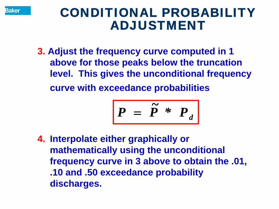
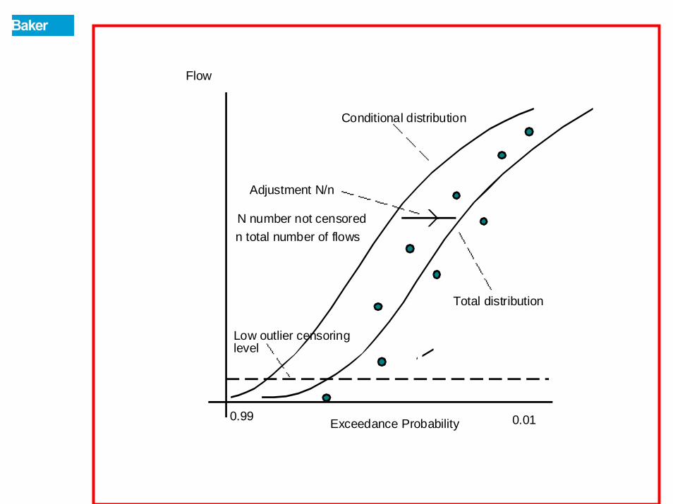
3. Adjust the frequency curve computed in 1 above for those peaks below the truncation level. This gives the unconditional frequency curve with exceedance probabilities P
4. Interpolate either graphically or mathematically using the unconditional frequency curve in 3 above to obtain the .01, .10 and .50 exceedance probability discharges.
dP*P~P =
Low outlier censoringlevel
Conditional distribution
Total distribution
Adjustment N/n
N number not censoredn total number of flows
Flow
Exceedance Probability0.99 0.01
CONDITIONAL PROBABILITY ADJUSTMENT
5. Compute the synthetic skew (GS ) standard deviation (SS) and mean ( ) using the three exceedance probabilities from 4 above and the following equations:
Where Q.01, Q.10 and Q.50 are discharges with .01, .10, and .50 exceedance probabilities and K.01, K.10, and K.50 are the corresponding Pearson Type III deviates.
6. The final step is to compute the weighted skew using GS computed in 5 above and the generalized skew G.
Rocky Arroyo at Hwy BRD near Carlsbad (station 08401900)
Computation of coefficient of skewness is needed in Bulletin 17B method of moments approach.
There is large uncertainty in computing coefficient of skewness for sample sizes commonly available in flood-frequency analysis.
Generalized skew is used to reduce uncertainty in estimating T-year events.
PLATE I IN BULLETIN 17B
• Map based on 2,972 stations that had 25 or more years of record through 1973 and drainage areas less than 3,000 square miles.
• Only 144 low outliers were found based on the Bulletin 17 (not 17B) low-outlier test that was not very sensitive.
• Historic flood information was not used.
• The national map has a mean-square error (MSE) of 0.302. Regional values of the MSEwould probably be more appropriate.
WEIGHTING THE SKEW COEFFICIENT
The weighted skew coefficient is computed as follows:
( ) ( )GG
GGW MSEMSE
GMSEGMSEG
++
=
WEIGHTING THE SKEW COEFFICIENT
The concept of weighting the station and generalized skew in proportion to their mean square errors was based on work by Tasker(1978).
GW = weighted skew coefficientG = station skew
= generalized skew= mean square error of generalized
skew= mean square error of station skew.
GGMSE
GMSE
WEIGHTING THE SKEW COEFFICIENT
The mean square error of the station skew (MSEG) can be determined from Wallis, Matalas, and Slack (1974). MSEG can be computed as:
MSEG = (Bias of skew coefficient)2 + variance of skew coefficient.
The bias and variance of station skew coefficients for Pearson Type III random variables can be obtained from Wallis, Matalas, and Slack (1974).
WEIGHTING THE SKEW COEFFICIENT
The following equation (Wallis, Matalas, and Slack (1974) is used for computing MSEG as a function of record length and skew
MSEG = 10 [A - B [LOG10 (N/10)] ]
Where A = -0.33 + 0.08 |G| if |G| < 0.90
-0.52 + 0.30 |G| if |G| > 0.90B = 0.94 - 0.26 |G| if |G| < 1.50
0.55 if > 1.50
Beard, L.R., 1974, Flood flow frequency techniques:Center for Research in Water Resources, TechnicalReport CRWR-119, The University of Texas, Austin,Texas. Benson, M.A., "Uniform Flood-Frequency EstimatingMethods for Federal Agencies," Water ResourcesResearch, Vol. 4, No. 5, Oct., 1968, pp. 891-908. Grubbs, F.E., and Beck, G., "Extension of Sample Sizesand Percentage Points for Significance Tests of OutlyingObservations," Technometrics, Vol. 14, No. 4, 1972, pp.847-854. Hardison, C.H., 1974, Generalized skew coefficient ofannual floods in the United States: Water ResourcesResearch, vol. 10, n0. 4, pp. 745-752.
REFERENCES
Interagency Advisory Committee on Water Data,1982, Guidelines for determining flood flowfrequency: Bulletin 17B of the HydrologySubcommittee, U.S. Geological Survey, Office ofWater Data Coordination, Reston, Virginia. Jennings, M.E., and Benson, M.A., 1969, Frequency Curves for Annual Flood Series with Some Zero Flow Events or Incomplete Data: Water Resources Research, Vol. 5, No. 1, pp. 276-280. National Academy of Sciences, 1978, Estimation ofpeak flows: prepared by the Task Force onEstimation of Peak Flows of the Panel on FloodStudies in Riverine Areas, Building ResearchAdvisory Board, National Research Council,Washington, DC, 10p.
Natural Environment Research Council, 1975,Flood Studies Report, Volume I – HydrologicalStudies, Water Resources Publications, FortCollins, Colorado. Tasker, G.D., 1978, Flood frequency analysis witha generalized skew coefficient: Water ResourcesResearch, vol. 14, no.2, pp. 373-376. Thomas, W.O., Jr., 1985, A uniform technique forflood frequency analysis: ASCE Journal of WaterResources Planning and Management, vol. 111,no. 3, pp. 321-327. Wallis, J.R., Matalas, N.C., and Slack, J.R., 1974,Just a moment!: Water Resources Research, vol.10, no. 2.