23/8/94 OCR Output Geneva, Switzerland simulations. structure. A recall of the theory is given before presenting the results of the beam dynamic An optics is also implemented in order to get the beam performances in the CLIC transfer produce bunches in the range of 10 nC with a c,bel0w 3 ps at the output of the bunch compressor. This note describes the design of a magnetic bunch compressor. The main objective is to pulses at the desired value when the energy is high enough. produce the requested high charges with a long pulse length, accelerate them and shorten the energy which were experimentally verified. In order to balance this effect, it is proposed to with high charge in short bunches. One of the limitations is the space charge effect at low The main goal of the CLIC Test Facility (CTF) is to study the generation of a drive beam Abstract F. Chautard, L. Rinolfi BUNCH COMPRESSOR FOR THE CLIC TEST FACILITY CERN—PS-94-30 CLIC Note 240 IIIIIIIIIIIIIIIIIIIIIIIIIIIIIIIIIIIIIIIIIIIIIIIIIIIIIIIIIIIII . I I CERMPS °°‘"3° Im CERN LIBRARIES, GENEVA CERN - PS DIVISION CERN EUROPEAN ORGANIZATION FOR NUCLEAR RESEARCH
Transcript
23/8/94 OCR Output
Geneva, Switzerland
simulations.structure. A recall of the theory is given before presenting the results of the beam dynamicAn optics is also implemented in order to get the beam performances in the CLIC transferproduce bunches in the range of 10 nC with a c,bel0w 3 ps at the output of the bunch compressor.
This note describes the design of a magnetic bunch compressor. The main objective is to
pulses at the desired value when the energy is high enough.produce the requested high charges with a long pulse length, accelerate them and shorten theenergy which were experimentally verified. In order to balance this effect, it is proposed towith high charge in short bunches. One of the limitations is the space charge effect at low
The main goal of the CLIC Test Facility (CTF) is to study the generation of a drive beam
Abstract
F. Chautard, L. Rinolfi
BUNCH COMPRESSOR FOR THE CLIC TEST FACILITY
CERN—PS-94-30CLIC Note 240IIIIIIIIIIIIIIIIIIIIIIIIIIIIIIIIIIIIIIIIIIIIIIIIIIIIIIIIIIIII . I I CERMPS °°‘"3° Im
CERN LIBRARIES, GENEVA
CERN - PS DIVISION
CERN
EUROPEAN ORGANIZATION FOR NUCLEAR RESEARCH
B Graphics 35 OCR Output
A.2 Magnetic field along LAS ........ - 34
A.1 PARMELA input listing ......... · 32
A PARMELA input Hles 32
Acknowledgements 31
Conclusion 31
4.4 Proposed settings for the 1995 CTF . . 30
..............43 Spectrometer line 29
4.2 Bunch compressor of ........... 29
.................41 New layout 28
CTF line 1995 28
3.4.4 Other improvements ....... 28
3.4.3 Longitudinal phase space .... 26
3.4.2 Beam envelopes and emittances . 22
223.4.1 Momentum spread fnmction of the charge
213.4 Results from PARMELA simulations .......
203.3 Optimisation of the phases. ............
203.2 Layout of simplified CTF line for simulations . .
193.1 Definition of the optics ...............
19Design of the CTF bunch compressor
............182.9.5 Choice for the CTF
..a-manet ................ 18294 Alphg
................. 18293 Helical wiggler
..anar wer ............... 17292 Pliggl
cane ................... 172.9.1 Chi
172.9 Review of other magnetic compressions .....
ance ............... 172.8 RMS beam emitt
152.7 Ellipse parameters in the longitudinal phase space
142.6 ecromeer oics .................Spttpt
132.5.3 Vertical matrix for beam optics .......
2.5.2 Horizontal matrix for beam optics .....2.5.1 Optical design ................
2.5 Magnetic compression with three dipoles ......
2.4 um uncenh ...............inimbh lgt
2.3 Principle of the longitudinal compression ......
2.2 Equivalcnce between particle phase Q and longitudinal position zons ..........................2.1 Variable definiti
30 56Horizontal beam envelopes with bunch compressor off.
29 55Mechanical layout of the bunch compressor region. . .. ...............
28 54Complete CTF line (1995)
ace care eect. ....................27 53Sphgff
26 52Longitudinal phase space at the TRS (5, 10 nC). . . .·• 5125 Longitudinal phase space at the TRS (0, 1, 3 nC). . .
24 50Longitudinal phase space evolution through the CTF line for a 10 nC beam.
4923 Longitudinal phase space evolution through the CTF line for a 5 nC beam.
4822 Longitudinal phase space evolution through the CTF line for a 3 nC beam.
4721 Longitudinal phase space evolution through the CTF line for a 1 nC beam.
4620 Longitudinal phase space evolution through the CTF line for a 0nC beam. .
19 (x,x’) and (y,y’) phase space evolutions through the CTF line for a 10 nC beam. 45
18 (x,x’) and (y,y’) phase space evolutions through the CTF line for a 0 nC beam. 444317 Vertical beam envelopes for the simplified CTF line. ....
4216 Horizontal beam envelopes for the simplified CTF line. . . .
4115 Vertical beam envelopes in the bunch compressor region. . .
4014 Horizontal beam envelopes in the bunch compressor region.
3913 Momentum spread function of the charge .......
e scannns an. ................ 3812 Phasigt 0 C
3711 Simplified CTF layout for simulations .........
3610 CTF optics in the bunch compressor region .......19Central trajectory in the bunch compressor ......16Evolution of a fnmction of K(B,·y)° ...........
ecromeer resouon ................. 15SpttltiBasic requirements for a simplined bunch compressor.
pe parameters ................Second diol
. .................First dipole parametersBasic geometry for a 3 dipole bunch compressor. . . .Ellipse parameters for the longitudinal phase plane. . .Compression process in the (Q, 6p) phase space ....
List of Figures
LIST OF FIGURES
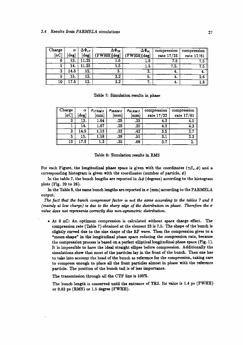
27 OCR OutputSimu.lati0n results in RMS ........
27Simulation results in phase .......
25Output data for 10 uC ..........
24Output data for 0 nC ..........
23Input data and transmission results ( ge- dependent )
23Input data (independent of the charge) .
20Magnet characteristics ..........
13a-dependence of main parameters ....
List of Tables
LIST OF TABLESiv
pi = p,, p,, p, is the momentum conjugate to the space coordinate.ej = qz, qv, q, is the space coordinate,c is the velocity of the light,
<I> and A are function of space and time,
where
H = ci> + - eA)’ + m’c’ (3) OCR Output
vector potential A, and scalar potential, ¢, is:
The Hamiltonian function for a charged particle of mass, m, and charge, e, in a magneticUnder these conditions the particles move in the phase space as in an incompressible fluid.
P = (2)8H
(1)BH
fnmction H(q,p, t)the system is conservative, one can derive the classical particle motion from the HamiltonianA group of particles are described by two sets of canonically conjugate variables q and p. If
2.1 Variable definitions
2 Analytical model
can be conserved up to the CLIC structure with a good emciency.simulations are analysed and show that the bunch characteristics at the compressor outputThe optics and the settings of the whole CTF line are given. Finally the beam dynamics
This note describes the principle of the magnetic bunch compressor based on 3 dipoles.(or even 20 MeV / c later on) and then longitudinally compressed down to 0, = 3 ps.at the RF gun with long laser pulses (0, = 8 ps). They will be accelerated up to 10 MeV/ ccharge is always below 2nC/bunch. A proposal [4] was made in order to produce high chargesExperiments done with different trains (8 bunches, 16 bunches, 24 bunches) show that the
Maximum charge at the CLIC structure: q= 7 nCMaximum charge at the gun exit: q= 14 nCe' pulse length at CLIC structure: 0, = 5.5 psLaser pulse length: 0, = 3.5 ps
Experiments done in the 1993 CTF run [3] are the following (for single bunch):0, = 1 mm.of 16 bunches has been made. It corresponds to 7 nC/bunch with the same brmch lengthshort bunch would be rather diflicult to produce and transport, a proposal [2] using a trainwith 0, = 3 ps crossing the R.F CLIC structure Since such a high charge in a singlesuch an electric field at 30 GHz, it would be necessary to produce a single bunch of 54 nCFor the CLIC machine, the nominal accelerating gradient is 80 MV / m. In order to generate
OCR Output1 Introduction
*For simplicity the variable q, from the Hamiltonian formalism is renamed z. OCR Output
Qg is the phase of the reference particle.to is the time of the reference particle,11, is the velocity of the particle,
»\ is the wavelength associated to the RF,w = 21rc/»\,is = Za/Vu
a particle i relativistic or not [7], wherebelow. The phase of the particle i is usually defined as Q, = —w(t, — to) + Q0 as the phase ofaccessible longitudinal variables are (Q, 6,7). The linear relation between ¢ and z I is recalledThe bunch compression studies are simulated with the code PARMELA [6] in which the
2.2 Equivalence between particle phase Q and longitudinal position z
conserved (Liouvi1le’s theorem).described by a set of two conjugate variables (q,, ,6,1) in which the longitudinal emittance istransverse plane in a sense that if the system is conservative then there exists a phase space
This transformation shows that the behaviour of the longitudinal plane is the same as thewhere B, = Q, / c
p. = Bnmc
considered where A, = A, = 0 Under this hypothesis (8) becomes:Only the longitudinal plane will be discussed here. Additionally, the equation (8) will be
Pa - ¢A. = Brrm¤ (8)
that one develops to get:
(p - eA)’ + m*c’(7),8= ·_%:.
(5 —¢A)’ 2 i·
From equation (4), the normalized velocity q/ c can be written as:
qi qi %6 (). · . 5 ‘ = " '*' ' *” + · "" p e eaem e;(<1,8428)
From (1) and (2) and expanding the equation (3) one obtains:
2 ANALYTICAL MODEL
SQ = ;; OCR Output
and
SQ = wgSz = Kpllll
term a,=O).One can compare both emittances by comparing the surfaces of the straight ellipses (coupling
,(14)71;7 + 2%(B.7)a + l31(B»‘1)¢z = €Q
Let 17 = ·2‘ll'/A in (12). Then (13) can be written as:
(13)viz? + 2¤¤zr(B.·y)t + @(6.7).2 = s.
transverse plane:ear combination of a generalisation of the Twiss parameters (ou, ,6,,7,) as it is done for theThe area e of the ellipse, which also represents the beam emittance, is described by a lin
Th¤r¢f¤r¢ Az = zi — zo = za A¢ = dn —¢¤ = ¢4 and 6p ¤= ((Bn)r — (»@.·1)¤—· (0.·7)téreference particle.
In all the following figures the phase spaces are centred in phase and momentum on thereference particle: zo = 0, to = 0 and (H,7)0.particles for example, where their coordinates and momentum are taken as a function of the
First, let us consider an ellipse in one of those phase spaces containing ninety per cent ofgiven below.the (z, ,8,7) or (Q, 6,7) phase spaces. A general formalism of the longitudinal compression isThe previous paragraphs demonstrated that the longitudinal emittance is conserved either in
2.3 Principle of the longitudinal compression
is the same as in (z, ,8,7).Finally, the variables (Q, @,7) are also a set of conjugate variables and the particle behaviour
(12)2 A AQ : -2
,6, : B0 2 1 andThe bunch compressor will work, at least, at 11 MeV, then particles will be relativistic:
s n¤ a11 ( )¢ = ·" —·····— + *1* U‘°(n °
21r Az 1 1
position of the particle i becomes z, = zo + Az. The expansion of (10) provides:lf zo is the longitudinal position of the reference particle in the bunch, then the longitudinal
,vi v0(10)Q- — Q ·—¢=()+ ¤gf " ’°
This yields to:
2.3 Principle of the longitudinal compression
K = ..1 (19) OCR Output
gives immediately a unique value of K:The optimum compression is reached when the ellipse has a horizontal waist. This condition
The equation (14) of the ellipse after the compression process becomes:to the momentum. Therefore the phase spread in the bunch will tend to a minimum.correlation, K should be determined in a such way that the change in phase is proportionalalso a linear transformation which implies a correlation between Q and 5,7. For a givenTh.is transformation conserves the momentum of the particle but modifies its phase. It isto the quantities after the transformation. K is an arbitrary constant (positive or negative).where the index, e, refers to the quantities before the transformation and the index, s, refers
(16)c 1)Qs : Qc — K z { (B (0.7). = (Bn).
adiabatic transformation (Fig. 1):From now on, the phase space (gb, 5,7) will be used. Let us apply to the ellipse the following
fe = ‘; (15)
The emittance being proportional to the surfaces, one obtains:
Figure 1: Compression process in the (Q, 6p) phase space
minimum phase spread of the bunch: 45,,,, and its symmetric f1·om the vertical axis. Then thethis point will change, so will K. Similarly, two points will determine, theoretically, theTherefore, (16:7),,,,,, is the ellipse reference point for an optimum compression and every time
71(21)-0.,,-K,/~§=0=>K=—2/i71
By substituting the expression of Q, into (20), one obtains:
= Ville
and
VB17Q,=—-ii-—Q ,,=>Q,=— m at \/E 71
The phase associated to (,6,7),,,,, is Q, which can be developed into:
Qs = QQ —
Assuming that K depends on the position of (,6,7),,,,,, the transformation (16) yields:
Figure 2: Ellipse parameters for the longitudinal phase plane.
CENTROID(him " 1/E
(llmax ' v/§
{ z I / l | V BY_ ¤¢max
'iint " / A {
slope-(§Y)max-,/E |. ..
Jay slo e ’ n - — p ~gy Q ‘l°m¤>< I - ;°
relation between K and these parameters is given below.The ellipse parameters (Fig. 2) for the longitudinal phase plane are derived from The
2.4 Minimum bunch length
2.4 Minimum bunch length
I, = p,[sin(e + cz) - sin(e + on + /9)] (24) OCR Output
ll = p,[sin(e + cx) - sine] (23)
I Magnet lengths (Fig. 4 and 5).
Figure 3: Basic geometry for a 3 dipole bunch compressor.
e+¤-I-B
B. i Y D . I ¤+¤+B
xs I l3M I xl
A,=1_,: the drift between the dipoles.p,=,__3: the curvature radius of the dipole,a, B,·y: the curvature angle of each dipole,l,=,__,: the length of each dipole,
quantities:
system with an angle e (Fig. 3). Its trajectory through those dipoles depends of elevenonly hard edge field is assumed. In the general case, a beam enters into the bunch compressorprocess. The following analytical study will not integrate the effect of the dipole fringe fields,This layout allows to keep the same momentum spread before and after the compression
2.5.1 Optical design
of three dipoles of inverse polarity. A study of such system is given below.For the reasons explained in Section 2.9.5, the choice for the CTF line is settled for a system
2.5 Magnetic compression with three dipoles
reduced to zero if 6p/p —> oo.momentum spread (~ 7; increases) for a constant emittance. Then, ideally, 45,,,, would beBecause of the Liouville’s theorem the positions of ¢,,,, can still be reduced by increasing the
2 ANALYTICAL MODEL
ll = psina (35) OCR Output
With the mentioned simpliiications, the expressions of the lengths become:
LM = 2p Sind + X (34)
I Longitudinal position associated to the maximum transverse deiectionz
D = 2p(1 — cosa) + Atana (33)
I Madmum transverse displacement:
P1:-P2=Ps=P¤¤dA1=A2=A (32)
Still willing to keep a symmetrical system we take:
d = (pl + p,)(1 — cos a) + (Al + A,)tana = 0 (31)
Additionally, we settle d to zero for reasons of symmetry:
(30)B=—(a+7)=7=a=|,6=—2a
compressor system. Thenassuming the beam to be parallel to the z-axis at the entrance and the exit of the bunch
e=0a.nde+¤+B+7=0
The problem is simplihed as follow:
dz d, +d,+d, -1-/\1ts¤(e+¤)+A,ta.¤(e+¤+B)]
transverse plane is:The total ofset in position between the input and the output of the bunch compressor in the
(29)da = p,[cos(e + a + B) — cos(e + a + B + 7)]
(28)dz = p¤[¤¤¤(¤ + ¤ + 5) - ¤¤¤(¤ + ¤=)l
(27)dl =p1[cose—cos(e+a)
the dipoles.
I In the transverse plane: ds = offset in position between the input and the output of
(26)L=l;+I¤+ls+A1+A,
The total length of the bunch compressor is:
(25)I3 = p8[sin(e+ ¤+B+·y)—si11(e+cx+B)]
2.5 Magnetic compression with three dipoles
Figure 5: Second dipole parameters OCR Output
p[1—cos(¤+p+ e)]
PU- ¤¤s(¤=|+ ¤)]¤+B
¤.+d+e yj
a+ s
§ I_¤+ e /p§<0
¤=i¤(¤+=) yp [si¤(¤+B+¤)]
(The third dipole is the same.)
Figure 4: First dipole parameters.
psi¤(e·•·u)
¤¤¤¤<¤+‘v)
Ella \ I l.¤xx(c+¤)e+¤
p[c¤se—cos(e+¤)]
psme
p[:in(e+¤)—si¤e]
2 ANALYTICAL MODEL
6p/pl I 6p/pl 0 OCR Output..1, = [MATRIX] I M
4x4 matrix formalism for the horizontal planedipole [B], an edge focusing [F] and a drift [D]. Each of them will describe the motion in athe matrix formalism. The bunch compressor is composed of three elementary matrices: aThe symmetry conditions for the lengths and magnetic field (Fig. 6) are used to develop
2.5.2 Horizontal matrix for beam optics
Figure 6 gives the simplified scheme.
B1:Bg=B3-TB
fields:
Since p = l/ sina and Bmp[,,,] z I{G,y),] /0.299, there is the following relations between the
Therefore:
(37)ls = p[¤i¤(¤+¤+·r)—¤i¤(¤+6)] = nsim
(36)I; = p[sincx — sin(—oz)] = 2p sine:
Figure 6: Basic requirements for a simplified bunch compressor.
21
"I' "-‘ r"—·I··‘····—·—·—-—--l--—--I-----I
2.5 Magnetic compression with three dipoles
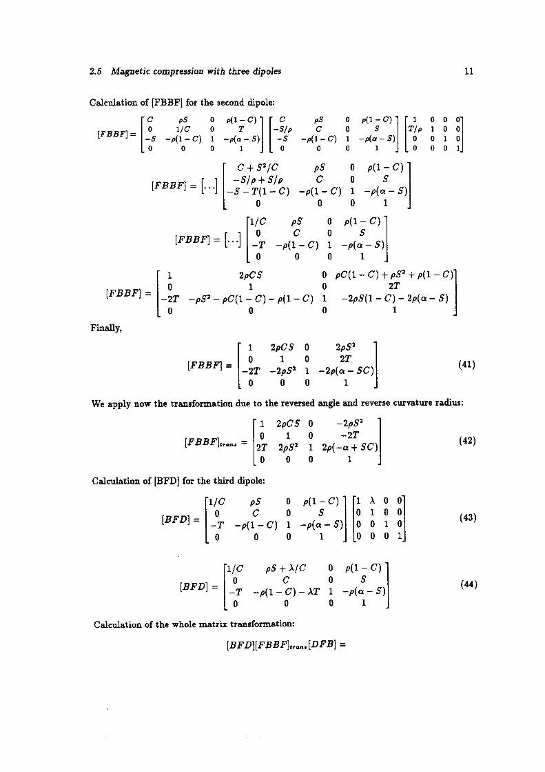
0 0 0 0 0 0 1 OCR Output
[D"]: (40)l l3 l 10 0/l{FB]: I.5 -psf?—C) 1 ·P(¤"S)1 A 0 C pS+A/C 0 ,v(1—$)+*\T
0 0 00
lFBl=|-s -p(1-0)0 TS+C
p(c¢S) l|—$ —p(1—6') S "P(°;"S)éS1;1- + T(g=C pS P(1·C)l lg *% 3 mf)
0 0 0 1|| 0 0 0 11 0| | -s -p(1—C) 1 -p(¤-S)
FB=[1I? 3 0 0| 1-s/p C 0 S1 0 0 ()`||' C pS 0 p(1·C)
Calculation of [DFB] for the Erst dipole:
calculation.
sign, the matrix of the central magnet will be taken as if it were positive and reversed aftera, and ctuvature radius, p, giving a total curvature angle of -2a. Because of their reversed
matrix calculation will begin and end with one dipole matrix.The edge focusing has no efect on a beam perpendicular to the dipole edge, then the
T as tana
S as sincz
C as cos a
We will use the following notations to lighten the matrix expressions:
6p/pz relative momentum spread.61, : path length diH`erence between the arbitrary ray and the central trajectory,z, z' : horizontal position and divergence,
The variables are:
[D] =
] [ 1 I 0FZ |tan_a/ p
p(a — sin a)_ [B] _ I — sina —-p(1 — cos a)sm cxsin u/p cos u
cos a p sma p(1 —— cos a)
The [MATRIX] elements are:
2 ANALYTICAL MODEL10
[BFD][FBBF],,,,,, [DFB] =
Calculation of the whole matrix transformation:
0 0 1
0 IBFDI = |-1——p(1 - 0) - ir 1 -p(¤ - s) (44) OCR OutputC 0 S
1/C pS+}\/C 0 p(1-C)
0 0 0 1 | |0 0 0 11-p(1-0) 1 —p(a—S)0 0 1 0[] (43)0 C 0 S 0 1 0 0 RFB- I* l I
1/C pS 0 p(1—C)`| [1 A 0 0
Calculation of [BFD] for the third dipole:
0 0 0 1
[FBBFl"···‘ Izr zps= 1 2p(-.1 + s0) (42)0 1 0 -2T
1 2pCS 0 -·2pS’
We apply now the transformation due to the reversed angle and reverse curvature radius:
of the momentum spread:the central particle and the arbitrary particle. We can now express these quantities function
This formalism can be extended to a bunch of particles in which one has to characteriseboth particles.and the central particle, A1, is the relative lengthening or shortening of the distance betweenSince 610 and 611 are respectively the initial and final distance between an arbitrary particle
0 -3TpS—%—=‘§-—€.-(1——C)+4pTS+!§-*—p(1—C) 1 A——p(a—.S')0 —CT + S
0 Bapr + ge + p
andB= @(1—C)+%`—-%-pT.S'+p(1—-C)Let: A = 2T(p(1 — C) + AT) + 2pT.5" — p(a — S) —— 2p
s 4rps+-p(1-c) 1 2T(p(1—C)+»\T)·+-2 rs° C ¤·—¤(¤=—-$)—2¤>(¤—$0)=[BFD] éi
p(1—C)+»\TC 3;:5+% 0
Which becomes,
0 0
25 — S 2T(pS + -2:) 1 2T(p(1 - C) + AT) + 2pTS° - p(¤— S) — 2p(¤— SC)
p(1-c)+1r+2ps°-1ps*c ps+g+zps o
2 ANALYTICAL MODEL12
curve _f(»\) starts to saturate. OCR OutputFrom this figure a possible position of the screen around l m is possible since the resolution
the curvature angle of the spectrometer: 0::30 degrees.one·ha1f of the horizontal beam divergence: z’0=2.4 mrad,one-half of the horizontal beam extent: ::0:1.3 mm,
Momentum spread: {$:3.8%,
the output data of PARMELA at the exit of the first dipole magnet at 0 nC:Figure 7 shows the evolution of f (A) for a beam with the following characteristics taken from
From both quantities, the resolution of the spectrometer is derived:The third term is the dispersion contribution (Disp).The first two terms are the emittance contribution (S igma,).
is switched on while the two others are off. From (40), the horizontal beam size at the exitWith the bunch compressor design, a spectrometer line will be implemented. The first dipole
Finally, the matrix transformation for the vertical plane is:
2 ANALYTICAL MODELOCR Output14
expression of cx and the magnetic field. For this purpose and since (,5,7),,,,, is the point OCR OutputWe have now to establish a relation between (52) and (51) at (6p/p),,,,, to determine the
<¤.¢>....,52 ‘ )¢¢ K : -—
note that both quantities ¢g and ¢, are the same and with (20), one has:one has to know the initial value 950 to calculate (51). (20) gives this information. One canAn optimum compression is obtained for ¢1=0, the two particles have the same phase. Then,cr. n. »\can vary the relative phase extension by changing the parameters of the bunch compressor:or shortening of the phase extension of the bunch. Once the momentum spread known oneAs written previously for the path length (see 2.5), ¢1-¢° represents the relative lengthening
2.7 Ellipse parameters in the longitudinal phase space
Figure 7: Spectrometer resolution
DIst•nc• from th• Hm dIpoI••xIt lm]
0 1 2 3 4
DI•plSIgm•x
152.7 Ellipse parameters in the longitudinal pbase space
beam. OCR Output
be applied to this bunch, corresponding to a magnetic field of B = 0.222 Tesla for a 20 MeVexample, at 0 nC, K (,8,7);, = 298.0 then a curvature angle of a = 30 degrees would have toK (B,7)0. Each different value of K is determined by the initial conditions of the bunch. Forcomputation will be required to extract the u value f1·om (53). Figure 8 shows a versusTo resolve this equation where a is unknown, a. numerical method is used. Finally, another
53 ( )2 -—1—-—= 41-— -+2Xt —-=KB, (p‘7)m“/(BMO [ ( ma ) ¤¤¤]w0 ( ‘r)¤tancx — oz 360dv, —¢>0
6(,8,·y),,,,, —> (B,·y),,,,,, the equation (51) becomes:Using the equations (35) and (52), and since the ellipse is centred around the reference particle
particular point of the ellipse:for an optimum compression (Fig. 1), we express the momentum spread function of this
Figure 8: Evolution of cz function of K (,6,7);,
K(Bzv)
20001000
20
so
40
$0
a ld°U'°°‘l
2 ANALYTICAL MODEL16
characteristic is essential for the CTF line having a strong limitation in space. OCR OutputThe compression factor per unit of length is higher than the other methods. This
can be very conservative, reducing the manufacturing and power supplies costs.superconducting quadrupoles needed for a-magnet. Accordingly, the size of the magnetsThe fields involved in those dipoles are weak, about 0.222 T at 20 MeV/ c, versus
cx·magnet compressor.
beam passes through the bunch compressor without seeing any field, contrary to theA system of three dipoles can be switched off if no compression is desired while the
with the following arguments:The choice of 3 dipoles with inverse polarity as a bunch compressor for CTF has been made
2.9.5 Choice for the CTF
superconducting device.typical parameters of the CTF gun, we reach a 25 to 30 Tesla/m gradient. This implies atonically from head to tail of the bunch contrary to the chicane and wiggler systems. WithThis system has to be used for bunches in which the particle momentum decreases mono
cz 4(59),~ __._¤ " E9 GK ’(%*")’
one can approximate the gradient to:In the particular case of a quadrupolar field, n=1, and for small bunch momentum spread,
(sw1. spm
the particle trajectory, 1,, scales with momentum, p, as:Alpha-magnet is a generic term describing a range of achromatic mirrors [14]. The length of
2.9.4 Alpha-magnet
proportional to the number of cells. Then the chicane is more emcient.compression stays proportional to the cube of the length of the unit of cell, but is onlyproportional to the cube of the length, while when adding cells as a planar wiggler, thewhich means that for similar values of the magnetic Held, the chicane gives a compression
Al, __ ,
for a. wiggler with N,,, period. Therefore,
N“pPA1, 2-—- B h K 22(e 0)
I° 6p °
2.9.3 Helical wigglcr
2 ANALYTICAL MODELOCR Output18
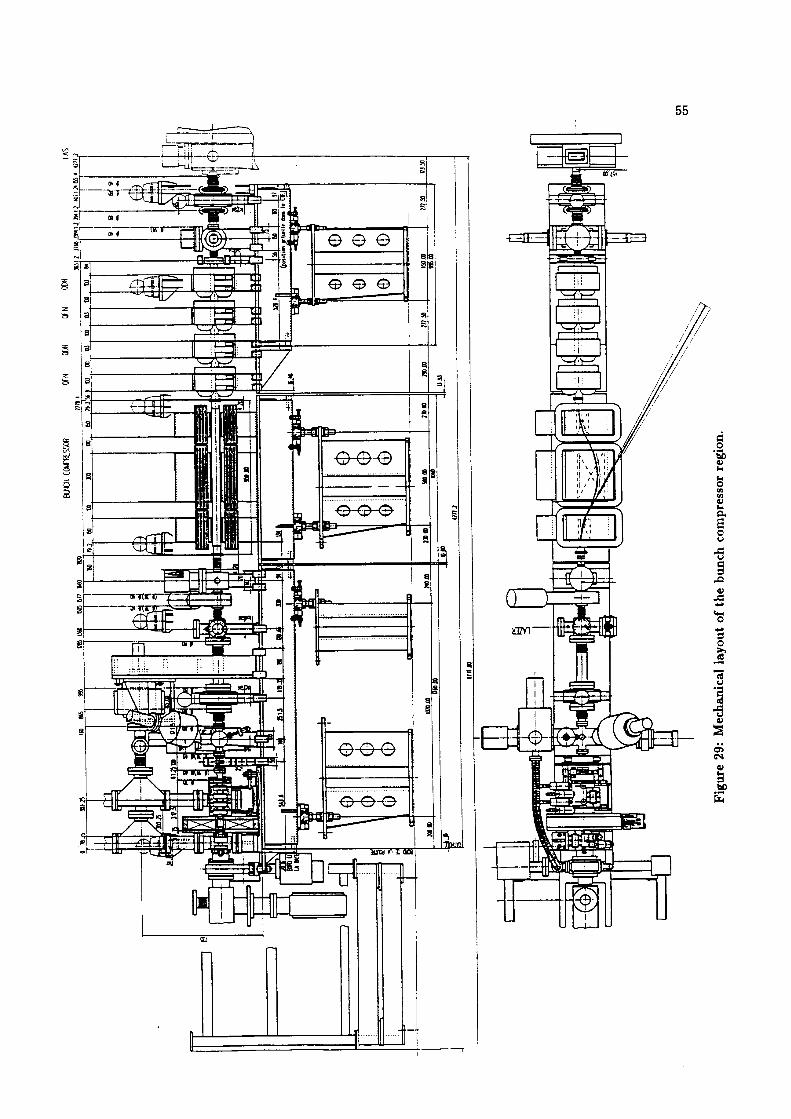
stimulating discussions [15]. OCR Output(Fig. 9). Uppsala University participated in the design of the bunch compressor and providedthese conditions, the trajectory of the reference particle in the bunch compressor is plottedfield will be: B = 0.223 T. The good field region covers the maximum requirements. Under
For a bunch compression at a maximum momentum of 20 MeV / c, the maximum magnetic
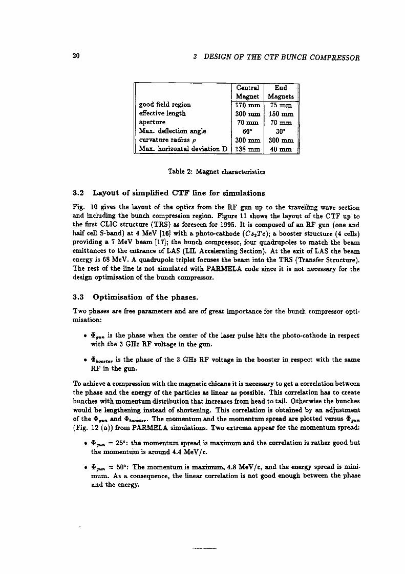
marises the characteristics discussed in the paragraph 2.5 for A: 100 mm.inverted polarity and full symmetry with respect to the central magnet axis. Table 2 sumAs mentioned above, the bunch compressor chosen for the CTF is based on 3 dipoles with
3.1 Definition of the optics
3 Design of the CTF bunch compressor
Figure 9: Central trajectory in the bunch compressor
Z [mm]
0 100 200 300 400 500 600 700 800
-0.1
Dipole 3Dipole 2005 if Dipolel
X 0.05
Q_] trajectory
particle
Reference
0.15
0.2
19
and the energy. OCR Outputmum. As a consequence, the linear correlation is not good enough between the phaseiw,. = 50°: The momentum is maximum, 4.8 MeV/ c, and the energy spread is mini
the momentum is around 4.4 MeV/ c.QW,. = 25°: the momentum spread is maximum and the correlation is rather good but
(Fig 12 (a)) from PARMELA simulations. Two extrema appear for the momentum spread:of the Q",. and @,6,;,,,. The momentum and the momentum spread are plotted versus iw,.would be lengthening instead of shortening. This correlation is obtained by an adjustment
bunches with momentum distribution that increases hom head to tail. Otherwise the bunches
the phase and the energy of the particles as linear as possible. This correlation has to createTo achieve a compression with the magnetic chicane it is necessary to get a correlation between
RF in the gim.•§y,,,,,,, is the phase of the 3 GHz RF voltage in the booster in respect with the same
with the 3 GHz RF voltage in the gun.• @9,,,, is the phase when the center of the laser pulse hits the photo-cathode in respect
misation:
Two phases are free parameters and are of great importance for the bunch compressor opti
3.3 Optimisation of the phases.
design optimisation of the bunch compressor.The rest of the line is not simulated with PARMELA code since it is not necessary for theenergy is 68 MeV. A quadrupole triplet focuses the beam into the TRS (Transfer Structure).emittances to the entrance of LAS (LIL Accelerating Section). At the exit of LAS the beamproviding a 7 MeV beam [17]; the bunch compressor, four quadrupoles to match the beamhalf cell S-band) at 4 MeV [16] with a photo-cathode (C.s;Tc); a booster structure (4 cells)the first CLIC structure (TRS) as foreseen for 1995. It is composed of an RF gun (one andand including the bunch compression region. Figure 11 shows the layout of the CTF up toFig. 10 gives the layout of the optics hom the RF gim up to the travelling wave section
3.2 Layout of simplified CTF line for simulations
Table 2: Magnet characteristics
40 mmMax. horizontal deviation D I 138 mm300 mm 300 mmcurvature radius p
30°60°Max. dehectiou angle
70 mm 70 mma.pe1·tu1·e
150 mm300 mmeffective length
170 mm 75 mmgood field regionMagnet Magnets
EndCentral
3 DESIGN OF THE CTF BUNCH COMPRESSOR20
cations to improve the transport of high charged beam toward the compressor system. After OCR OutputThe possibility to add another identical booster is still open. We rely on these two modifi
Additionally, the booster will increase ·y up to 21.5 corresponding to ,6 equal to 0.9989.hitting on the photo·cathode.force. This is achieved by working on the natural length of the laser pulse, am., = 16 ps,By lengthening the electron bunch one decreases the particle density po, so is the space charge
• Increase the beam energy.
• Increase the bunch length at the input of the bunch compressor.
were required to improve the compression process:compressor would be difficult to compensate needing strong quadrupoles. Two modificationsa growing repelling effect of this force. The induced beam divergence at the exit of the bunchbunch compression the distance between each particle becoming smaller, pg increases causing
The space charge effect has to be limited as much as possible because in the case of thewhen 7 increases.
Then the repelling electrostatic force is increasingly compensated by the magnetic forceB, is the azimuthal magnetic field derived from Ampere’s law V >< B = ifpov.
beam axis,
E, is the radial electrical field from Coulomb’s law VE = 4·xp0 at the distance 1· from the
where
Tv 21rep F, = e(E, — EB,) = gr
the velocity v along the z-axis:charge force F, in the simple case of a beam with a uniform particle density po moving withenvelope more critical. To understand how evolves this effect, one can characterise this spacedoes not take into account the effect of the space charge, making the matching of the beam11). This fitting is done by using the code TRANSPORT Nevertheless, TRANSPORTup the element parameters to obtain a maximum transmission all through the CTF line (Fig.0 nC, 1 nC, 3 nC, 5 nC and 10 nC. The simulations without space charge will allow to setSeries of simulations are done to investigate the bunch compression for different beam charges:
3.4 Results from PARMELA simulations
I-{ = 3.8%
Giving,
¢b¤o•t•r = 2640
¢,,,, = 25°
beam:
energy loss. According to the Figure 12, the following set of phases is chosen, for a 0 nCA compromise has to be found between the maximum momentum spread and a minimum
spread is close to its<I·,,,,,,, (Fig. 12 (b),(c)). One can notice that at the maximum momentum, the momentumFor these two extrema of §,,,,, the momentum and the momentum spread are plotted versus
21
that the main losses, for 10 nC, are due to LAS aperture, mainly in the vertical plane. OCR Output(Fig. 16) and in the vertical plane (Fig. 17) for the same set of initial charges. One can see
The beam envelopes are now plotted from the RF gum until TRS in the horizontal plane
87%.
whole CTF line for a charge below 10 nC. For this latter value, the transmission drops toThe results of the simulations show that a transmission of 100% is possible through the
the booster are described as ideal cosine functions. The number of macro particles is 300.and the distribution of the magnetic field along LAS. The electric iields in the RF gum and
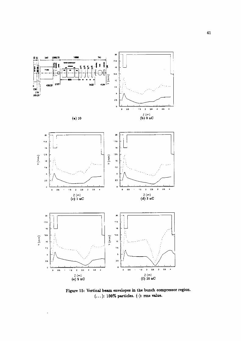
The Appendix A gives the files which are used as input files for PARMELA simulationsare dependent of the charge. Table 5 and 6 give the output data.Table 3 gives the input data which are independent of the charge and Table 4 those whichnot completely for a beam of 10 nC (particularly for the vertical plane).input). As shown on Figures 14 and 15, these conditions are reached for a beam of 0 nC butthe entrance of LAS with a beam radius equal or less than 12 mm (iris aperture at the LASThe settings of the four quadrupoles are optimised in order to have a minimum divergence atis kept for all lower charges.Its effect is clearly seen in the various plots. The optimised value found for the charge 10 nCThe only solenoid SNF350 allows to focus as good as possible the beam at the booster input.
element are drawn.
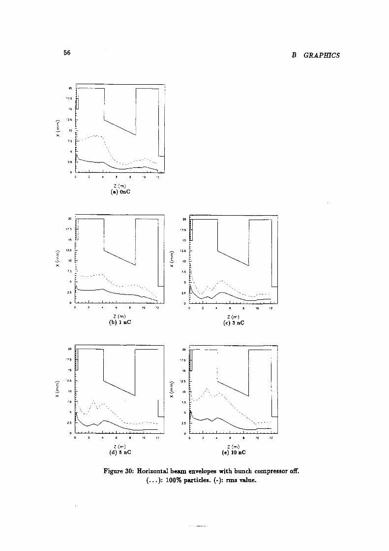
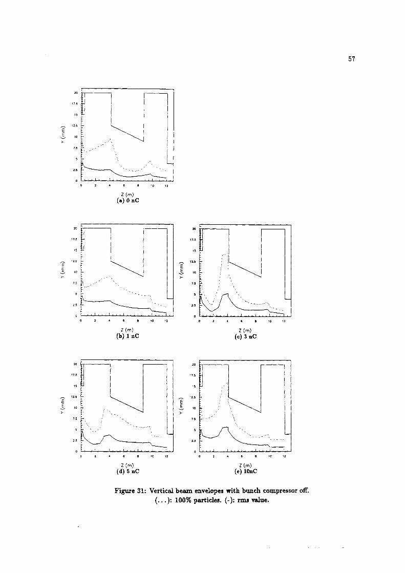
the region of the bunch compressor. On the same graphs, the aperture limitations of eachThese envelopes are restricted to the LAS input in order to analyse with better accuracy
0, 1, 3, 5, 10 nC.plane (Fig. 14) and in the vertical plane (Fig. 15) for the following initial charges:The beam envelopes from the RF gun until the entrance of LAS are reported in the horizontal
3.4.2 Beam envelopes and emittances
line.
Fortunately this value is still acceptable to keep a minimum beam loss through the CTFfor 0 nC, up to 1 % for 10 nC.high charge. However at the exit of LAS, the effect is inverted. 6p/p increases from 0.55%0 nC down to 3.55 % for 10 nC. The consequence will be a bunch compressor less efiicient atAt the exit of the booster (entrance of the bunch compressor), 6p/ p drops from 3.84 % for
• At the LAS exit (Fig. 13 (c))
• At the booster exit (Fig. 13 (b))
• At the gun exit (Fig. 13 (a))
The momentum spread versus the charge is plotted, for 46,,,,, = 25° and ¢b,,,,,,, : 264°value depends on the charge.The optimum 6p/p=3.8% corresponds to a beam without space charge effects. However this
3.4.1 Momentum spread function of the charge
completely ultra-relativistic.and the entrance of LAS in which the bunch length will be frozen when the beam becomescompression, one has to minimise the distance between the exit of the bunch compressor
3 DESIGN OF THE CTF BUNCH COMPRESSOR
Table 4: Input data and transmission results (charge-dependent) OCR Output
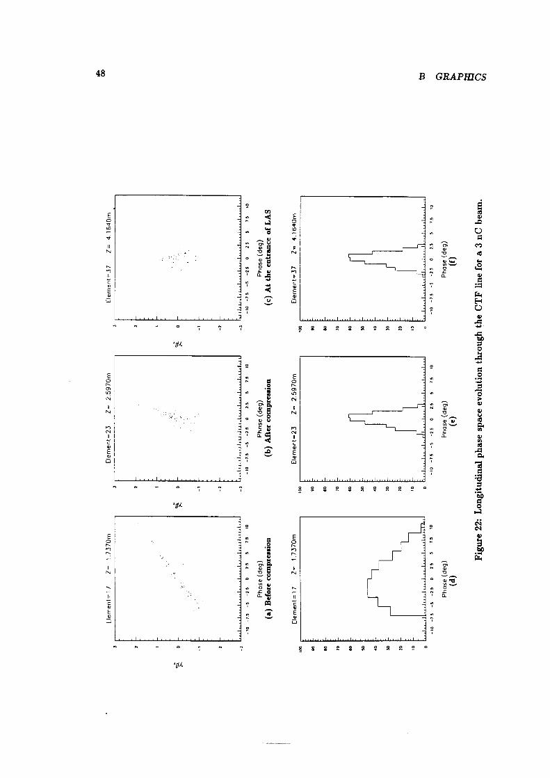
The longitudinal phase spaces are plotted at the 4 elements mentioned above:
• At the entrance of TRS: element 61.
• At the entrance of LAS: element 37.
• At the bunch compressor output: element 23.
• At the bunch compressor input: element 17.
particular places of the CTF (Fig. 11):In order to optimise the bunch compressor, the longitudinal phase space is analysed in four
3.4.3 Longitudinal phase space
charges.
LAS. However at TRS, both transverse phase spaces have decent values for such highcompensate this effect before entering in LAS and therefore 13% losses are produced indivergence at the bunch compressor exit. The consequence is that the quadruplet cannotthe bunch compressor input in both planes, there is a tremendous effect for the verticalAt 10 nC, the space charge effects are predominant and with a minimum divergence at
shape is recovered in both planes and with acceptable values.and vertical planes at the exit of the bunch compressor (Table 5). In TRS, the butterhysettings (Table 4), it has been possible to obtain the same emittances for the horizontalAlthough both transverse planes are not completely similar, with the proposed opticare increased, due to the fact that the horizontal dispersion is not completely cancelled.bution (butterdy shape). After the bunch compressor the horizontal beam dimensionsAt 0 nC, only the RF fields and the magnetic fields contribute to this particular distri
(F1g_ 19) at three different critical places of the CTF.Finally, the transverse phase spaces are characterised at 0 nC (Fig. 18) and at 10 nC
one of the goals of this study.However, 100% of particles can be focused correctly in the TRS for all charges which is
3 DESIGN OF THE CTF BUNCH COMPRESSOR
or 0.83 ps (RMS) or 1.5 degree OCR OutputThe bunch length is conserved until the entrance of TRS. Its value is 1.4 ps (FWHH)
The transmission through all the CTF line is 100%.
particle. The position of the bunch tail is of less importance.to compress enough to place all the front particles almost in phase with the referenceto take into account the head of the bunch as reference for the compression, taking caresimulations show that most of the particles lay in the front of the bunch. Then one hasIt is impossible to have the ideal straight ellipse before compression. Additionally thethe compression process is based on a perfect elliptical longitudinal phase space (Fig. 1).“moon·shape” in the longitudinal phase space reducing the compression rate, becauseslightly curved due to the sine shape of the R.F wave. Then the compression gives to acompression rate (Table 7) obtained at the element 23 is 7.5. The shape of the bunch is
• At 0 nC: An optimum compression is calculated without space charge effect. The
value does not represents correctly this non-symmetric distribution.(mainly at low charge) is due to the sharp edge of the distribution in phase. Therefore the crThe fact that the bunch compressor factor is not the same according to the tables 7 and 8
output.
In the Table 8, the same bunch lengths are reported in 0 according to the PARMELA
plots (Fig. 20 to 26).In the table 7, the bunch lengths are reported in A¢ (degrees) according to the histogram
corresponding histogram is given with the coordinates (number of particle, ¢»)For each Figure, the longitudinal phase space is given with the coordinates (·yB,,¢) and a
Table 8: Simulation results in RMS
3.710 I 17.5 I 1.3 I .35 I .68
3.1 2.35 I 15. I 1.18 I .38 I .51
3.5 2.73 I 14.5 I 1.13 I .32 I .42
4.3 4.31 I 14. I 1.07 I .25 I .25
4.54.20 I 13. I 1.04 I .25 I .23rate 17/61I¤CI I [des} I [mm] I [mm} I [mm] I me 17/23
The 30 GHz RF power generated in TRS is sent to the CAS (CLIC Accelerating Structure). OCR OutputThe complete layout of the CTF as foreseen for 1995 is given (Fig. 28).
gradients equal to 80 MV/m.Another objective is to check that an acceleration with such RF power is possible with
pulses in order to check the generation of 30 GHz RF power.As already mentioned, one of the CTF objectives is to produce short and intense electron
4.1 New layout
4 CTF line 1995
compression rate would be improved.The “moon-shape” in the phase space at low charge would be reduced. Therefore the
• A higher electric field in the gun and in the booster would improve the overall scheme.
optimise the phase of LAS to improve the compression.higher momentum spread is obtained by changing ¢,,,, and 4:,,,,,,,. Then it remains to38% and 7% respectively, inducing a larger phase spread, QM, after compression. AAt the exit of the gim and at the exit of the booster 6p/ p gets smaller, in a. range of6p/ p (see 2.4). However, the opposite effect occurs when the charge increases (Fig. 13).
• For a given bunch length, the compressed brmch length can be minimised by increasing
3.4.4 Other improvements
which allows to keep a short bunch with high charge at TRS input.Further simulations are done in order to understand this eject and find a correct setting
appears when a magnetic field is superimposed on the accelerating structure (LASphysical phenomenon or simply a numerical eject from PARMELA. This bunch lengtheningbecomes of the order of 10° at the TRS input (Fig. 26 It is not yet clarified if it is a
Although the bunch length is in the range of 5° at the entrance of LAS (Fig. 24 (c)}, itis explained by a not completely optimised angle cz for 5 nC.
The cr of the compressed bunch length at 5 nC, is greater than at 10 nC ( Table 8}. This
momentum spread.grow ( see scatter plots (c) in Figures 20 to 24). Figure 13 shows the evolution of theAfter compression when the correlation almost disappeared the momentum spread willbunch compressor these phenomena will first reduce the momentum spread of the beam.plots (a) in Fig. 20 to 24). Then, for a non·relativistic bunch in the drift before theBoth phenomena tend to rotate the phase space clockwise ( see evolution of the scatterparticles of the beam, while the particles in the tail are decelerated for the same reason.particles in the f1·ont of the beam are accelerated by the repulsive force f1·om the otherterises its effect on a compressed beam at 3 nC. The phenomenon is the following: TheThe space charge forces introduce a longitudinal emittance growth. Figure 27 charac
dipoles is increased with the charge.different charge in order to get a maximum transmission (Table 4). The field in theof the beam after compression. The settings of the quadrupoles are changed for eachvaried. Only the four quadrupoles would have to compensate the very strong divergence
• With charge: The optics before the bunch compressor stay the same when the charge is
4 CTF LINE 1995
spectrometer line. OCR Output
These values are optimised for a good matching in the Faraday cup and a good resolution as
y; :2.3 mradyl :1.4 mm
2:Q :22.3 mradZ1 IIIID
The beam characteristics at this point and at 0 nC are:of 700 mm downstream the exit of the first dipole.simulations with TRANSPORT code give a distance for a screen, followed by a Faraday cup,of the Faraday cup is 35 mm. In order to transport all the beam to the Faraday cup, thederived from Fig. 7. The vacuum chamber is 60 mm in the horizontal plane. The apertureand Fig. 29). A scintillator screen will be installed in the line and the optimised position isIn order to measure some beam characteristics, a spectrometer line is implemented (see 2.6
4.3 Spectrometer line
According to the simulations, the 1995 CTF line could work without the bunch compressor.gun up to TRS input.
Fig 30 and 31 show respectively the horizontal and vertical beam envelopes from the RFPARMELA simulations have been performed under this hypothesis.
system without any loss when this latter is off.and with a train of bunches, one should transport the beam through the bunch compressor
For the set-up of the CTF, at least at low energy and for specific studies, in single bunchcompression is strongly recommended.was working continuously. However, the option to accelerate beam in LAS without anyUp to now, design and simulations have been presented assuming that the bunch compressor
4.2 Bunch compressor off
It is now designed and mechanical pieces are ordered according to this configuration.Fig. 29 shows the mechanical layout of the bunch compressor region.
efficiency factor , it would be possible to get 80 MV/ m in the CAS.bunches, corresponding to an electric field of 113 MV /m in TRS. Taking into account the
From the simulations, one can expect to produce 60 MW peak in TRS, with the compressed
Edu 1].3
charge Q 3 nCAt (FWHH) 3.3 ps
1.4 ps
0.42 mm
TRS e" pulse length
5.8 A
9.2 A
4. A
1.45 T/m—2.3 T/m
Triplet 1. T/mBLAS 0.1 T
RF power 30 MW
Eus 17 MV/m
LAS ¢;,A$ 2 350°
2.4 A
1.4 A
0.8 A
2.8 A
-0.59 T/m0.34 T] m-0.19 T/m
Quadruplet 0.70 T / m
22.6 A
22.6 A
0.056 T
Bunch compressor cz 14.5°
RF power 8.3
Eb°°,g,,
Booster ¢a».m¢¤· 264°
69. A
SNF350 0.24 T
RF power 6.0
E,,,,, 100 MV/m
¢,,,,, 25°
energy 0.2 mJ
Laser pulse length : 19 ps
(At low charges)
4.4 Proposed settings for the 1995 CTF
30 4 CTF LINE 1995 OCR Output
of the bunch compressor. OCR Outputcode PARMELA. D. Reistad (Uppsala University) gave a valuable contribution to the designsen, A. Riche. B. Mouton and W. Remmer provided a great help for the improvements of thethe CTF beam dynamics working group: H. Braun, J .P. Delahaye, G. Guignard, J .H.B. MadA number of people made very usefiil comments and suggestions to this study. In particular
6 Acknowledgements
install the bunch compressor in the CTF at the beginning of 1995.the entire system before the end of the year in order to do the magnetic measurements andbunch compressor has been finalised and the order has been placed. It is foreseen to receiveTRS. In consequence and based on these simulation results, the mechanical design of the
Under these conditions, the total transmission is close to 90% until the CLIC structureobjective to produce and accelerate single bunches of 10 nC and 0, { 3 ps is reached.of the system to the geometric aberrations and chromatic effects is in progress. The mainThis note is the first step in the design of the bunch compressor for the CTF. The sensitivity
31
1000.0 OCR Output
1000.0
1000.0
1000.0
1000.0
1000.0
1000.0
1000.0
1000.0
1000.0
1000.0
1000.0,
1000.0
1000.0
1000.0
1000.0
1000.0
1000.0
1000.0
1000.0
1000.0,
1000.0
1000.0
1000.0,
1000.0
1000.0,
800.0
600.0
400.0
200.0
50.0
10.0
S champ chp=value of this field can be modulated by a factor ’COEFF’ in FOCLAL.by the use of a FOCLAL card. This card calls the file ’bzfield’ given below. Additionally, theA magnetic field along LAS, represented by the TRWAVE cards, can be switched on and off
sections and an intermediate focusing solenoid. CERN/PS 93-26 (RF}, CLIC note 206[17] R. Bossart, J .C. Godot, S. Liitgert, A. Riche. Modular RF grm consisting of two RF
the CLIC Test Facility. Linac Conference 1992, CERN/PS 92-48 (LP), CLIC note 183P. Marchand, L. Rinolfi. Beam dynamics simulations in the photo—cathode RF gun for[16]
[15] F. Chautard. Minutes of the meeting held on 17 March 1994. PS/LP/Note 94-12 {Min.}
Note 91-42C.D. Johnson, J. Str6de. An alpha magnet for the CLIC Test Facility. CERN/PS/LP[14]
held on 01-07-93
R. Corsini. Helical wiggler for bimch compression. Minutes of the CTF Theory meeting[13}
S. Kheifets et al. Bunch compression for the TLC: preliminary design. SLA C-P UB-4 802[12]
Meeting in Japan. Tsukuba. 1993compression for femto-second single pulse. Proceedings of the 18th Linear AcceleratorM. Uesaka, T. Kozawa, Y. Yoshida, T. Kobayashi, T. Ueda and K. Miya. Magnetic pulse[111
pressors for iutur linear colliders. SLAC-PUB-6119T.O. Raubenheimer, P. Emma and S. Kheifcts. Chicane and wiggler based bunch com[10]
T.P. Wangler. Introduction to linear accelerators. Los Alamos Laboratory. LA- UR-93-805[9]
for designing charged particle beam transport systems. CERN 80-04K.L Brown, D.C. Carey, Ch. Iselin and F. Rothacker. Transport. A computer program[8]
M. Borland. A high-brightness thermionic microwave electron grm. SLA C-Report-4 02[7]
B. Mouton. The PARMELA program (Version 4.3). LAL/SERA 93-455[6]
School, April 1987E.J.N Wilson. Nonlinear resonances. In Proceedings of the 1985 CERN Accelerator[5]
CERN linear collider test facility (CTF). NIM A340 (1994} 139-145[4] J .P. Delahaye, J .H.B. Madsen, A. Biche and L. Rinolii. Present status and future of the
comments. PS/LP/Note 94-07H. Braun, J.H.B. Madsen and S. Schreiber. The CTF nm N ° 4 -1993- Results and[3]
K. I-Iilbner. Generation of 30 GHz power in the CLIC Test Facility. CLIC note 134[2]
J .P. Delahaye. A simplified scheme for 30 GHz RF generation in CTF. CLIC note 175[1]