97
Business 33001: Microeconomics Owen Zidar University of Chicago Booth School of Business Week 2 Owen Zidar (Chicago Booth) Microeconomics Week 2 1 / 97

Business 33001:Microeconomics
Owen Zidar
University of Chicago Booth School of Business
Week 2
Owen Zidar (Chicago Booth) Microeconomics Week 2 1 / 97

Today’s Class
1 Consumer and Producer Surplus
2 Efficiency
3 Government Intervention in the Economy
4 Taxes and RegulationEfficiencyIncidence
Owen Zidar (Chicago Booth) Microeconomics Week 2 2 / 97

Motivation: why should you care?
1 Understand how much market participants, both consumers andproducers, benefit from consuming or producing a certain good
Relevant for consumer satisfaction and loyaltyRelevant from valuing existing firms and innovation
2 Deepen your insight into and influence on the debate over economicpolicy, taxation, and regulation
Private-sector managers are better able to position their organizations,both defensively and offensively, if they understand why and howgovernments actExceptional private-sector leaders are now widely expected to provideinformed, intelligent leadership on the policy issues
Owen Zidar (Chicago Booth) Microeconomics Week 2 3 / 97

Consumer Surplus
Owen Zidar (Chicago Booth) Microeconomics Week 2 4 / 97

Consumer Surplus
Definition
Consumer surplus is an individual’s gain from trade or simply total valueminus total expenditure (i.e., the amount she is willing to pay minus thequantity she actually had to pay)
Owen Zidar (Chicago Booth) Microeconomics Week 2 5 / 97
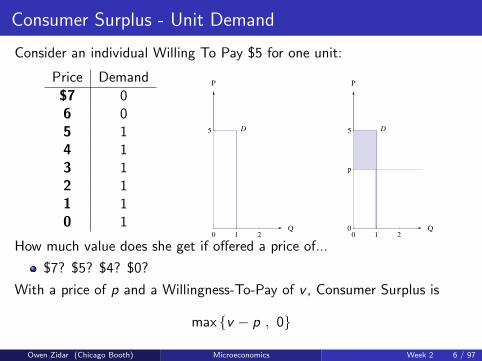
Consumer Surplus - Unit Demand
Consider an individual Willing To Pay $5 for one unit:
Price Demand
$7 06 05 14 13 12 11 10 1
0 1 2Q
5
P
D
0 1 2Q0
p
5
P
D
How much value does she get if offered a price of...
$7? $5? $4? $0?
With a price of p and a Willingness-To-Pay of v , Consumer Surplus is
max {v − p , 0}
Owen Zidar (Chicago Booth) Microeconomics Week 2 6 / 97

Consumer Surplus - Unit Demand
Multiple consumers:
Values v1 = 6, v2 = 4, v3 = 2
Price p = 3
CS: (6− 3) + (4− 3) = 4
Price D1 D2 D3
$7 0 0 06 1 0 05 1 0 04 1 1 03 1 1 02 1 1 11 1 1 10 1 1 1
0 1 2 3Q0
p
v1
v2
v3
P
D
0 1 2 3Q0
p
v1
v2
v3
P
D
CS
General Rule: Consumer Surplus is Area below Demand, above Price
Owen Zidar (Chicago Booth) Microeconomics Week 2 7 / 97

Consumer Surplus - Non-Unit Demand
Individual Consumer:
Willing to buy up to 3 units
Willing to pay v1 = $6 for first ; v2 = $4 for second; v3 = $2 for third
Price P = 3
Price Demand
$7 06 15 14 23 22 31 30 3
0 1 2 3Q0
p
v1
v2
v3
P
D
0 1 2 3Q0
p
v1
v2
v3
P
D
CS
CS = (6− 3) + (4− 3) = 4
No difference: Area between demand curve and price line
Owen Zidar (Chicago Booth) Microeconomics Week 2 8 / 97

Consumer Surplus
Height of demand curve at Q tells us willingness to pay for Qth unit(for individual or in aggregate)
Q
P
p
q
DA
B
(A+B) Area under demand curve: Total value of units up to q
(B) Area under price line: total cost paid for units up to q
⇒ (A) Area between demand and price: Consumer Surplus
Owen Zidar (Chicago Booth) Microeconomics Week 2 9 / 97

Consumer Surplus
Q
P
p
q
DCS
Linear Demand ⇒ CS is the area of a triangle
CS = 12 × base × height
General Demand: Integrate to find area
Integrate PD(Q)− P∗ from Q = 0 to Q = Q∗
(PD(Q) is the “inverse demand”)
Owen Zidar (Chicago Booth) Microeconomics Week 2 10 / 97

Consumer Surplus
Consumer Surplus: “Triangle under Demand Curve”
0 50 100 150 200Q0
10
20
30
40
50
P
p
q
DCS
Demand Curve: QD(P) = 250− 5PSuppose P = 30, so Q = 100. What is CS?
Area of triangle =1
2· 100 · 20 = 1000
Suppose price increases to P = 40. What is the change in CS?
New CS =1
2· 50 · 10 = 250, Change is − 750
Owen Zidar (Chicago Booth) Microeconomics Week 2 11 / 97

Consumer Surplus Application #1: Google users
Back of the Envelope
Time using library treatment = 22 + travel
Time using web = 7
Questions per day now = 1 per capita
Answerable questions per day = 12 per capita
Questions per day then = close to zero
Problem
When getting answers was expensive we asked few questions
Now that getting answers is cheap we ask a lot of questions
Owen Zidar (Chicago Booth) Microeconomics Week 2 12 / 97

Consumer Surplus Application #1: Google users
Demand curve for questions
minutes
Questions per day
22+
7
1/2
Owen Zidar (Chicago Booth) Microeconomics Week 2 13 / 97

Consumer Surplus Application #1: Google users
Consumer surplus
minutes
Questions per day
22+
7
1/2
Area = base x height/2 = 15/4 = 3.75 minutes
Owen Zidar (Chicago Booth) Microeconomics Week 2 14 / 97

Consumer Surplus Application #1: Google users
Per Person
Average hourly earnings = $22
Save 3.75 minutes per day = $1.37/day
365 days in a year = $500
How many users?
130M people employed 130M x 500 = $65B
300M population 300M x 500 = $150B
Owen Zidar (Chicago Booth) Microeconomics Week 2 15 / 97

Consumer Surplus Application #1: Google users
Summary
Value to users in time saved ≈ $65B
Leaves out
Cost of trips to library
Unanswerable searches
Value to non-employed
Value of better matched purchases
Entertainment value
Improved decisions
Etc, etc, etc.
Owen Zidar (Chicago Booth) Microeconomics Week 2 16 / 97
Revealed Preference
“Revealed Preference”: By observing individual’s buying behavior(purchase or not), we can determine his or her value for a good
If the price is $P and you buy, value is at least $P
If the price is $P and you don’t buy, value is at most $P
If you don’t buy at $P+.01 and you buy at $P-.01, value is $P
Owen Zidar (Chicago Booth) Microeconomics Week 2 17 / 97

Revealed Preference
“Revealed Preference”: By observing individual’s buying behavior(purchase or not), we can determine his or her value for a good
$45/month X X∼ $500/month X X
Owen Zidar (Chicago Booth) Microeconomics Week 2 18 / 97

Revealed Preference
“Revealed Preference:” By observing demand curve, we can determinesociety’s value for a good
One point on curve: If 1000 people buy at price $7, society’s value for1000 units is at least $7000
Full curve: we see when every person starts buyingAdd it all up to get consumer surplus
0 50 100 150 200Q0
10
20
30
40
50
P
p
q
DCS
Owen Zidar (Chicago Booth) Microeconomics Week 2 19 / 97

Consumer Surplus Application #2: Toll Roads
Alice and Bob both drive to work on a highway
Tolls on the highway jump up by $20 per trip
Alice keeps driving, Bob stops
Who is made more worse off by the toll hike?
Does it matter if I tell you Alice is rich and Bob is poor?Does it matter if I tell you Bob’s job lets him work from home now?Does it matter if I tell you Bob was already thinking of retiring?Does it matter if I tell you Bob switched to a super-slow bus?
What about a fast bus, with great wifi?
If we accept that dollars are equal across people, willingness to paycaptures all information
Owen Zidar (Chicago Booth) Microeconomics Week 2 20 / 97

Consumer Surplus Application #3: Gentrification
Owen Zidar (Chicago Booth) Microeconomics Week 2 21 / 97

Consumer Surplus Application #3: Gentrification
Owen Zidar (Chicago Booth) Microeconomics Week 2 22 / 97

Consumer Surplus Application #3: Gentrification
Questions:
What is the economic logic behind the sentiment: “my neighborhoodgot better, this sucks?”
What can we infer about the effects on former residents if they moveout?
How can we relate gentrification to the toll road example?
How can we relate gentrification to supply and demand?
Owen Zidar (Chicago Booth) Microeconomics Week 2 23 / 97

Producer Surplus
Owen Zidar (Chicago Booth) Microeconomics Week 2 24 / 97

Producer Surplus (Profit)
Individual Firm:
Can produce up to 3 units
Cost of c1 = 2 for first unit; c2 = 4 for second; c3 = 6 for third
Price p = 5
Price Supply
$7 36 35 24 23 12 11 00 0
0 1 2 3Q0
p
c1
c2
c3
P
S
0 1 2 3Q0
p
c1
c2
c3
P
S
PS
PS = (5− 2) + (5− 4) = 4
What if c1 = 4, c2 = 2, c3 = 6? New Supply and PS?
Owen Zidar (Chicago Booth) Microeconomics Week 2 25 / 97

Producer Surplus
Height of supply curve at Q tells us cost of production of Qth unit(for firm or industry)
Q
P
p
q
S
A
B
(B) Area under supply curve: Total cost of producing units up to q
(A+B) Area under price line: Total revenue from selling units up to q
⇒ (A) Area between price and supply: Producer Surplus (Profit)
Owen Zidar (Chicago Booth) Microeconomics Week 2 26 / 97

Producer Surplus
Q
P
p
qS
PS
Linear Supply ⇒ PS is area of a triangle
PS = 12 × base × height
General Supply:
Integrate P∗ − PS(Q) from Q = 0 to Q = Q∗
(PS(Q) is the “inverse demand”)
Owen Zidar (Chicago Booth) Microeconomics Week 2 27 / 97

Producer Surplus
Producer Surplus: “Triangle above Supply Curve”
0 50 100 150 200Q0
10
20
30
40
50
P
p
qS
PS
Supply Curve: QS(P) = 5P − 50Suppose P = 30, so Q = 100. What is PS?
Area of triangle =1
2· 100 · 20 = 1000
Suppose price increases to P = 40. What is the change in PS?
New PS =1
2· 150 · 30 = 2250, Change is + 1250
Owen Zidar (Chicago Booth) Microeconomics Week 2 28 / 97

Producer Surplus Application #1: Uber Driver
Suppose an uber driver was willing to drive today
Owen Zidar (Chicago Booth) Microeconomics Week 2 29 / 97

Producer Surplus Application #2: Airlines and 9/11
How much did 9/11 hurt the airline industry?
Owen Zidar (Chicago Booth) Microeconomics Week 2 30 / 97

Producer Surplus Application #2: Airlines and Sept 11
In 2000, p = 122, q = 148 M passangers who got on a plane
After 9/11, p = 104, q = 125 M
Areas A+B in the prior slide amounted to $2.3 B in lost PS
Source: Goolsbee, Levitt, Syverson Fig 3.6
Owen Zidar (Chicago Booth) Microeconomics Week 2 31 / 97

Efficiency
Owen Zidar (Chicago Booth) Microeconomics Week 2 32 / 97

Definition: Economic Efficiency (Pareto Optimality)
Definition
An allocation of society’s resources is efficient if there is no otherallocation that would make someone better off without harming others.
Owen Zidar (Chicago Booth) Microeconomics Week 2 33 / 97

Efficiency from a managerial perspective
Think of yourself as managing a large (or small) business organization.
Your job is to allocate the business’s resources such as its capital andemployees in order to achieve a goal–say maximizing shareholdervalue.
If by changing the way you do things–say by shortening the workweekor providing stronger incentives to the sales force–you can increaseshareholder wealth without harming employees, then the changeenhances efficiency.
Similarly, if some hypothetical change in procedures would makeemployees better off without harming shareholder wealth, then thatchange would also enhance efficiency. In other words, an efficientorganization satisfies Pareto’s definition.
Owen Zidar (Chicago Booth) Microeconomics Week 2 34 / 97

The Condition for Economic Efficiency
Resources are efficiently allocated when the marginal value of each goodor service is equal to the marginal cost of producing it.
Owen Zidar (Chicago Booth) Microeconomics Week 2 35 / 97

Consumer + Producer Surplus
p
P
S
D
CS
PS
Market equilibrium produces the right quantityAt quantity Q: (Height of D) - (Height of S) = Value - CostLeft of q: Value > CostRight of q: Value < Cost
The market equilibrium allocates this quantity correctlyConsumers: any buyer has higher WTP than any nonbuyerFirms: Any unit produced has a lower cost than any unit that isn’t
Market equilibrium maximizes total surplus (PS+CS)
Owen Zidar (Chicago Booth) Microeconomics Week 2 36 / 97

Gas Rationing after Hurricane Sandy
After Hurricane Sandy, quantity of gas in NY/NJ limited in the short run
What happens in this market?
p
P
S
D
Normal Supply & Demand
p
P
S
S'
D
Sandy supply shockOwen Zidar (Chicago Booth) Microeconomics Week 2 37 / 97

Gas Rationing after Hurricane Sandy
“Equilibrium Market Price” spikes way above “Fair Price”
State Accuses 13 New York Gas Stations ofPrice-Gouging (NYT, 11/15/2012):
The stations accused of price-gouging charged $4.74 to $5.50a gallon in the days after the storm. Just before the storm, theaverage price for gasoline in New York City was about $3.91 agallon... After Tropical Storm Irene, a Yonkers gas station thathad raised its price by 97 cents a gallon agreed to pay a $7,500penalty.
Other policy responses to ration gas:Odd/Even rationing of gas salesFederal Government ships in gas, generators for gas stationsNat’l Guard gives away free gasWaive gas taxes
Do these policies solve the problem? Any other ideas?Do these policies create any new problems?
Owen Zidar (Chicago Booth) Microeconomics Week 2 38 / 97

Gas Rationing after Hurricane Sandy
Gas Rationing is New Burden After Hurricane Sandy(NYTimes 11/3/2012): Tony Kurasz sat in his sport utilityvehicle for three hours on Saturday at an Exxon station inBayonne, N.J.; he was six cars away from the pump when thestation ran out of gas. It was his second gas line of the day. Thefirst station ran out, too.
What would have happened with a free market?
Who are the winners and losers from the non-free market policy?
Owen Zidar (Chicago Booth) Microeconomics Week 2 39 / 97

Gas Rationing after Hurricane Sandy
Price Caps, Quantity Controls:
General problems:
Long linesBlack market?Misallocation to consumers
Can’t get gas when you “need” it
Poor incentives for suppliers
Short run: Bring in goods from outside, at a high costLong run: Build infrastructure / stock extra for extreme events
Rent controlled buildings, cabs, subsidized heating bills...Putting all the costs and benefits together,a free market is best – even after a hurricane. (Maybe)
Owen Zidar (Chicago Booth) Microeconomics Week 2 40 / 97

Hurricane Sandy
After the hurricane, the market equilibrium has high prices for gas.
Are high prices inherently bad?
A dollar in gas station’s hand = a dollar in consumer’s handGiven a transaction, price is irrelevant to surplusMaximizing surplus is all about getting correct transactions to occur
Perfect allocation to consumers
Gas goes to highest value usersNo waiting in line, no wasted time
Perfect incentives to firms
If supply is perfectly inelastic, irrelevantIf we can bring in extra fuel at some cost, market prices give the“right” incentives
Bring if and only if cost is below marginal consumer’s value (WTP)
Owen Zidar (Chicago Booth) Microeconomics Week 2 41 / 97

Government Intervention
Owen Zidar (Chicago Booth) Microeconomics Week 2 42 / 97

Government Intervention in the Economy
Organizing framework: “ When is government intervention necessaryin a market economy?”
Market first, government second approach
Why? Private market outcome is efficient under a broad set ofconditions (1st welfare theorem)
This section can be split into two parts
How can govt. improve efficiency when private market is inefficient?
What can govt. do if private market outcome is undesirable due todistributional concerns?
Owen Zidar (Chicago Booth) Microeconomics Week 2 43 / 97
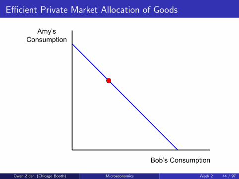
Efficient Private Market Allocation of GoodsE¢cient Private Market Allocation of Goods
Amy’sConsumption
Bob’s Consumption
Public Economics Lectures () Part 1: Introduction 37 / 49Owen Zidar (Chicago Booth) Microeconomics Week 2 44 / 97

First Role for Government: Improve EfficiencyFirst Role for Government: Improve E¢ciency
Amy’sConsumption
Bob’s Consumption
Public Economics Lectures () Part 1: Introduction 38 / 49Owen Zidar (Chicago Booth) Microeconomics Week 2 45 / 97

Second Role for Government: Improve DistributionSecond Role for Government: Improve Distribution
Amy’sConsumption
Bob’s Consumption
Public Economics Lectures () Part 1: Introduction 39 / 49Owen Zidar (Chicago Booth) Microeconomics Week 2 46 / 97

First Welfare Theorem
Private market provides Pareto efficient outcome under three conditions
1 No externalities
2 Perfect information
3 Perfect competition
This theorem tells us when government should intervene
Owen Zidar (Chicago Booth) Microeconomics Week 2 47 / 97

Failure 1: Externalities
Markets may be incomplete due to lack of prices (e.g. pollution)
Achieving an efficient solution requires an organization to coordinateindividuals – that is, a government
This is why govt. funds public goods (highways, education, defense)
Questions: What public goods to provide and how to correctexternalities?
Owen Zidar (Chicago Booth) Microeconomics Week 2 48 / 97

Failure 2: Asymmetric Information and Incomplete Markets
When some agents have more information than others, markets fail1 Adverse selection in health insurance
Healthy people drop out of private market → unravelingMandated coverage could make everyone better off
2 Capital markets (credit constraints) and subsidies for education3 Markets for intergenerational goods
Future generation’s interests may not be fully reflected in marketoutcomes
Owen Zidar (Chicago Booth) Microeconomics Week 2 49 / 97

Failure 3: Imperfect Competiton
When markets are not competitive, there is role for govt. regulation
Ex: natural monopolies such as electricity and telephones
We will discuss monopolies later in the course
Owen Zidar (Chicago Booth) Microeconomics Week 2 50 / 97

Individual Failures
If agents do not optimize, government intervention (e.g. by forcingsaving via social security) may be desirable
This is an “individual” failure rather than a market failure
Conceptual challenge: how to avoid paternalism
Why does government know what is desirable for you (e.g. wearing aseatbelt, not smoking, saving more)
Difficult but central issues for optimal policy design
Owen Zidar (Chicago Booth) Microeconomics Week 2 51 / 97

Redistribution Concerns
Even when the private market outcome is efficient, may not havegood distributional properties
Efficient markets generally seem to deliver very large rewards to asmall set of people (top incomes)
Government can redistribution income through tax and transfersystem
Owen Zidar (Chicago Booth) Microeconomics Week 2 52 / 97

Why Limit Government Intervention?
One solution to these issues would be for the government to overseeall production and allocation in the economy (socialism).
Serious problems with this solution1 Information: how does government aggregate preferences and
technology to chose optimal production and allocation?2 Government policies distort incentives (behavioral responses in private
sector)
In practice, there are sharp tradeoffs between the costs and benefitsof government intervention
Owen Zidar (Chicago Booth) Microeconomics Week 2 53 / 97

Equity-Efficiency TradeoffEquity-E¢ciency Tradeo§
Amy’sConsumption
Bob’s Consumption
Public Economics Lectures () Part 1: Introduction 47 / 49Owen Zidar (Chicago Booth) Microeconomics Week 2 54 / 97

Taxes
Owen Zidar (Chicago Booth) Microeconomics Week 2 55 / 97

Outline
1 Example Tax Problem
2 EfficiencyKey lessons about efficiency costs of taxation
3 Equity3 key lessons about tax incidence
Applications
Owen Zidar (Chicago Booth) Microeconomics Week 2 56 / 97

Per-Unit Taxes (Math)
General Approach:
Demand QD(PD), Supply QS(PS)Without taxes:
Set PS = PD
Set QS = QD
With per-unit tax of t:Set PS = PD − tSet QS = QD
Specific Example:
Demand: QD(PD) = 50− 2PD , Supply: QS(PS) = 3PS − 15Without taxes:
Quantity q = 24Prices PD = PS = p = 13
With per-unit tax of t = 5:Plug in PS = PD − 5Quantity q′ = 18Demand price PD = p′ = 16Supply price PS = p′ − t = 11
Owen Zidar (Chicago Booth) Microeconomics Week 2 57 / 97

Per-Unit Taxes (Math Example – ctd)Demand QD(PD) = 50− 2PD , Supply QS(PS) = 3PS − 15
18 24Q
5
111316
25
PD
No taxes: q = 24, p = 13Consumer Surplus: 1
2 · 12 · 24 = 144Producer Surplus: 1
2 · 8 · 24 = 96
Tax of t = 5 per unit: q = 18, pD = 16, pS = 11Consumer Surplus: 1
2 · 9 · 18 = 81 – loss of 63Producer Surplus: 1
2 · 6 · 18 = 54 – loss of 42Government Revenue: 18 · 5 = 90
Net loss of surplus: 63 + 42− 90 = 15
Owen Zidar (Chicago Booth) Microeconomics Week 2 58 / 97

Taxes
p
p�t
PD
S
D S'
t
Market Equilibrium with Taxes
Owen Zidar (Chicago Booth) Microeconomics Week 2 59 / 97

Taxes
p
p�t
PD
S
D S'
CS
PS
t
Market Equilibrium with Taxes
Consumer Surplus
Producer Surplus
Owen Zidar (Chicago Booth) Microeconomics Week 2 60 / 97

Taxes
p
p�t
PD
S
D S'
CS
PS
REV
t
Market Equilibrium with Taxes
Consumer Surplus
Producer Surplus
GovernmentRevenue
Owen Zidar (Chicago Booth) Microeconomics Week 2 61 / 97

Taxes
p
p�t
PD
S
D S'
CS
PS
REV DWL
t
Market Equilibrium with Taxes
Consumer Surplus
Producer Surplus
GovernmentRevenue
Deadweight Loss
Owen Zidar (Chicago Booth) Microeconomics Week 2 62 / 97

Deadweight Loss
Deadweight Loss is the “economic cost” of a tax
Taxes paid are not lost – they go to Gov’t
The loss is in transactions which don’t go through
Firm willing to produce a good for a price of $10Consumer willing to pay $11Transaction would create $1 in surplus
Tax of < $1: transaction goes through, no lossTax of > $1: no transaction, loss of $1
Marginal cost (extra DWL) of taxation increasing in the tax rate:
Say that every dollar of taxation reduces quantity by one unitTaxes go from 0 to 2 dollars per unit:
kill 2 transactions, each of surplus about $1Taxes go from $99 to $101:
kill 2 transactions, each of surplus about $100
Approximately 100 times as bad!
Owen Zidar (Chicago Booth) Microeconomics Week 2 63 / 97

Deadweight LossMarginal cost of taxation increasing in the tax rate
Q
P
t
�Q
DWL
Deadweight loss is approximately quadratic in the tax amount
DWL = 12 t ·∆Q
∆Q proportional to t (for linear supply & demand)So DWL goes as t2
Owen Zidar (Chicago Booth) Microeconomics Week 2 64 / 97

Deadweight LossMore elastic supply & demand ⇒ More DWL
Two markets with same P & Q, but different supply and demand curves:
Q
P
t
�Q
DWL
Q
P
t
�Q
DWL
For a given tax t, DWL is bigger if supply & demand are more elasticDWL = 1
2 t ·∆QMore elastic supply and demand mean larger ∆Q for a given tIntuition: DWL is caused by loss of transactionsMore elastic S&D means more transactions destroyed
Owen Zidar (Chicago Booth) Microeconomics Week 2 65 / 97

Tax Policy Implications
With many goods, most efficient way to raise revenue is:
1 Tax inelastic goods more (e.g. medical drugs, food)
2 Spread taxes across all goods to keep rates relatively low on all goods(broad tax base)
These are two countervailing forces; balancing them requires quantitivemeasure meant of deadweight loss
Owen Zidar (Chicago Booth) Microeconomics Week 2 66 / 97

Efficiency and equity consequences of taxation
Definition
Efficiency costs: effect of policies on size of the pie
Focus in efficiency analysis is on quantities, not prices
Incidence: effect of policies on distribution of economic pie
Owen Zidar (Chicago Booth) Microeconomics Week 2 67 / 97

Incidence
Definition
Tax incidence is the study of the effects of tax policies on prices and thedistribution of utilities
Owen Zidar (Chicago Booth) Microeconomics Week 2 68 / 97

Incidence
Ideally, we would characterize the effect of a tax change on utilitylevels of all agents in the economy
Useful simplification in practice: aggregate economic agents into afew groups
Incidence analyzed at a number of levels:1 Producer vs. consumer (tax on cigarettes)2 Source of income (labor vs. capital)3 Income level (rich vs. poor)4 Region or country (local property taxes)5 Across generations (social security reform)
Owen Zidar (Chicago Booth) Microeconomics Week 2 69 / 97

Key Lessons about Tax Incidence
1 Economic tax incidence separate from “legal incidence”
2 Taxing consumers and producers results in same economic impact1
1If taxes are fully salient (Chetty, Looney, Kroft (2009)). Recall ∆PB = ∆PS + τOwen Zidar (Chicago Booth) Microeconomics Week 2 70 / 97

D
S
B
Price
Quantity
$22.5$22.5
$19.5
D+t
$7.50
$27.0
$15.0$15.0
A
1250 1500
D
C
Tax Levied on Consumers
ConsumerBurden = $4.50
SupplierBurden = $3.00
Public Economics Lectures () Part 2: Tax Incidence 13 / 140
Owen Zidar (Chicago Booth) Microeconomics Week 2 71 / 97

ConsumerBurden = $4.50
D
S
B
SupplierBurden = $3.00
Price
Quantity
$22.5$22.5
$19.5
$27.0
A
1250 1500
S+t
$7.50
$30.0
Tax Levied on Producers
C
D
Public Economics Lectures () Part 2: Tax Incidence 14 / 140
Owen Zidar (Chicago Booth) Microeconomics Week 2 72 / 97

Analytical Framework
We know a three things:2
%∆PD = %∆PS + τ
%∆QD = εD%∆PD
%∆QS = εS%∆PS
We also have market clearing:
%∆QD = %∆QS
εD%∆PD = εS(%∆PD − τ)
2where ∆Q is the percentage change in quantity generated by the tax and τ is alsomeasured in percentage terms.
Owen Zidar (Chicago Booth) Microeconomics Week 2 73 / 97
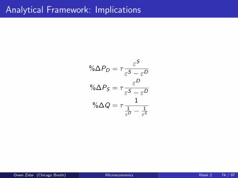
Analytical Framework: Implications
%∆PD = τεS
εS − εD
%∆PS = τεD
εS − εD
%∆Q = τ1
1εD− 1
εS
Owen Zidar (Chicago Booth) Microeconomics Week 2 74 / 97
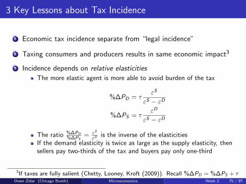
3 Key Lessons about Tax Incidence
1 Economic tax incidence separate from “legal incidence”
2 Taxing consumers and producers results in same economic impact3
3 Incidence depends on relative elasticities
The more elastic agent is more able to avoid burden of the tax
%∆PD = τεS
εS − εD
%∆PS = τεD
εS − εD
The ratio %∆PD
%∆PS= εS
εDis the inverse of the elasticities
If the demand elasticity is twice as large as the supply elasticity, thensellers pay two-thirds of the tax and buyers pay only one-third
3If taxes are fully salient (Chetty, Looney, Kroft (2009)). Recall %∆PD = %∆PS + τOwen Zidar (Chicago Booth) Microeconomics Week 2 75 / 97

$27.0
$22.5
1500
DS
S+t
$7.50
Quantity
Price
Consumerburden
Perfectly Inelastic Demand
Public Economics Lectures () Part 2: Tax Incidence 15 / 140Owen Zidar (Chicago Booth) Microeconomics Week 2 76 / 97

SS+t
Quantity
Price
D
$7.50
Supplierburden
1500
$22.5
$15.0
Perfectly Elastic Demand
Public Economics Lectures () Part 2: Tax Incidence 16 / 140
Owen Zidar (Chicago Booth) Microeconomics Week 2 77 / 97

Example from my research on corporate tax incidence
“Who Benefits from State Corporate Tax Cuts? A Local Labor MarketsApproach with Heterogeneous Firms”
Owen Zidar (Chicago Booth) Microeconomics Week 2 78 / 97
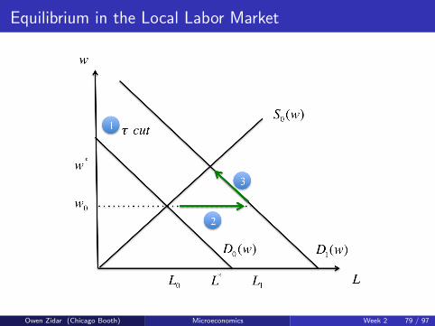
Equilibrium in the Local Labor Market
Owen Zidar (Chicago Booth) Microeconomics Week 2 79 / 97

Equilibrium in the Local Labor Market
Owen Zidar (Chicago Booth) Microeconomics Week 2 80 / 97

Regulation Example: Mandated Benefits
We have focused until now on incidence of price interventions (taxes)
Similar incidence/shifting issues arise in analyzing quantityintervention (regulations)
Leading case: mandated benefits – requirement that employers payfor health care, workers compensation benefits, child care, etc.
Mandates are attractive to government because they “off budget”;may reflect salience issues
Owen Zidar (Chicago Booth) Microeconomics Week 2 81 / 97

Mandated Benefits
Tempting to view mandates as additional taxes on firms and applysame analysis as above
But mandated benefits have different effects on equilibrium wagesand employment differently than a tax (Summers 1989)
Key difference: mandates are a benefit for the worker, so effect onmarket equilibrium depends on benefits workers get from the program
Unlike a tax, may have no distortionary effect on employment andonly an incidence effect (lower wages)
Owen Zidar (Chicago Booth) Microeconomics Week 2 82 / 97

Mandated Benefits: Simple Model
Labor demand (D) and labor supply (S) are functions of the wage w
Initial equilibrium:
D(w0) = S(w0)
Now government mandates employers provide a benefit with cost t
Workers value the benefit at αt dollars
Typically 0 < α < 1 but α > 1 possible with market failures
Labor cost is now w + t, effective wage w + αt
New equilibrium:
D(w + t) = S(w + αt)
Owen Zidar (Chicago Booth) Microeconomics Week 2 83 / 97

Mandated Benefit
w1
L1
D1
S
A
WageRate
Labor Supply
Public Economics Lectures () Part 2: Tax Incidence 130 / 140
Owen Zidar (Chicago Booth) Microeconomics Week 2 84 / 97

w1
L1
D1
S
D2
$1
A
WageRate
Labor Supply
Mandated Benefit
B
Public Economics Lectures () Part 2: Tax Incidence 131 / 140
Owen Zidar (Chicago Booth) Microeconomics Week 2 85 / 97

w2
w1
L1
D1
S
D2
$1
A
WageRate
Labor Supply
$α
C
Mandated Benefit
B
Public Economics Lectures () Part 2: Tax Incidence 132 / 140
Owen Zidar (Chicago Booth) Microeconomics Week 2 86 / 97

Mandated Benefits Application: Disabilities Act
The 1993 Americans with Disabilities Act requires employers to:
Make accommodations for disables employeesPay same wages to disables employees as non-disabled workers
Cost to accommodate disabled workers: $1000 per person on average
Theory is ambiguous on net employment effect because of wagediscrimination clause
Owen Zidar (Chicago Booth) Microeconomics Week 2 87 / 97

w2
w1
L1
D1
S
D2
AB
WageRate
Labor Supply
minimum wage
Mandated Benefit with Minimum Wage
Public Economics Lectures () Part 2: Tax Incidence 136 / 140
Owen Zidar (Chicago Booth) Microeconomics Week 2 88 / 97

Mandated Benefits Application: Disabilities Act
Employment of disabled workers fell after the reform (roughly 5-10%)
Wages did not change
Results consistent with a labor demand elasticity of −1 or −2.
ADA intended to help those with disabilities but appears to have hurtmany of them because of wage discrimination clause
Underscores importance of considering incidence effects beforeimplementing policies
Owen Zidar (Chicago Booth) Microeconomics Week 2 89 / 97

Wrapping Up
p
p�t
PD
S
D S'
CS
PS
REV DWL
t
MarketEquilibrium with Taxes
Consumer Surplus
Producer Surplus
GovernmentRevenue
Deadweight Loss
Owen Zidar (Chicago Booth) Microeconomics Week 2 90 / 97

Supplemental Material
Owen Zidar (Chicago Booth) Microeconomics Week 2 91 / 97

Outline
1 Efficiency Costs
2 Subsidies
3 Externalities
Owen Zidar (Chicago Booth) Microeconomics Week 2 92 / 97

Efficiency Cost: Properties
1 DWL increases with square of tax rate
2 DWL increases with elasticities
Owen Zidar (Chicago Booth) Microeconomics Week 2 93 / 97

DWL is a triangle
Base of the triangle (measured vertically) is the change in prices: τP
The height of the triable (measured horizontally) is the change inquantities: Q%∆Q
Social Cost is:
=1
2τPQ (%∆Q)
=1
2τPQ
(τ
11εD− 1
εS
)
=1
2τ2 PQ︸︷︷︸
Tax Revenue
(1
1εD− 1
εS
)
Social Cost from increasing taxes is: d(Social Cost)dτ = τTR
(1
1
εD− 1
εS
).
Owen Zidar (Chicago Booth) Microeconomics Week 2 94 / 97

Subsidies
Subsidies are negative taxes
PD < PS : Buyer pays less than seller receives
Inefficiency: Too many trades
Increase CS and PS, Negative government revenue
Firm willing to produce a good for a price of $10Consumer willing to pay $9Subsidy of < $1: no transaction, efficient outcomeSubsidy of > $1: transaction goes through, economic loss of $1
CS + PS goes up by less than cost to government
Owen Zidar (Chicago Booth) Microeconomics Week 2 95 / 97

Subsidies
Subsidy (negative tax) of r per unit:
pS
pD
P
r
AB
C
DE F
Consumer surplus: C + B + D
Producer surplus: A + B + E
Cost to government: B + E + D + F
Net Surplus:(C + B + D) + (A + B + E )− (B + E + D + F ) = A + B + C − F
Surplus without a subsidy: A + B + C
Deadweight Loss: FOwen Zidar (Chicago Booth) Microeconomics Week 2 96 / 97

Externalities
Externalities: byproducts of market transactions which affect others
Negative externalities: my purchase or production hurts others
Factories emit pollution, alcohol leads to crime, antibiotic overuseGoods with negative externalities are overprovided by the marketWe can discourage production with Taxes, Production caps
Positive externalities: my purchase or production helps others
Knowledge spillovers, Vaccinations, Plastic Surgery (?)Goods with positive externalities are underprovided by the marketWe can encourage production with Subsidies, Mandates,
or Creation of property rights (patents)
Not an externality – part of the market:
You are better off because I buy a good from youYou are worse off because I bought a good you wantedMarket outcome still efficient
Owen Zidar (Chicago Booth) Microeconomics Week 2 97 / 97


