55
Business Systems Intelligence: 5. Classification 1 D r . B r i a n M a c N a m e e ( w w w . c o m p . d i t . i e / b m a c n a m e e )
| Date post: | 20-Dec-2015 |
| Category: |
Documents |
| View: | 216 times |
| Download: | 2 times |

Business Systems Intelligence:
5. Classification 1
Dr. B
rian Mac N
amee (w
ww
.comp.dit.ie/bm
acnamee)

2of25
2of55 Acknowledgments
These notes are based (heavily) on those provided by the authors to
accompany “Data Mining: Concepts & Techniques” by Jiawei Han and Micheline Kamber
Some slides are also based on trainer’s kits provided by
More information about the book is available at:www-sal.cs.uiuc.edu/~hanj/bk2/
And information on SAS is available at:www.sas.com

3of25
3of55 Classification & PredictionToday we will look at:
– What are classification & prediction?– Issues regarding classification and prediction– Classification techniques:
• Case based reasoning (k-nearest neighbour algorithm)• Decision tree induction• Bayesian classification• Neural networks• Support vector machines (SVM)• Classification based on association rule mining concepts• Other classification methods
– Prediction– Classification accuracy

4of25
4of55 Classification & PredictionClassification:
– Predicts categorical class labels– Classifies data (constructs a model) based on
the training set and the values (class labels) in a classifying attribute and uses it in classifying new data
Prediction: – Models continuous-valued functions, i.e.,
predicts unknown or missing values
Typical Applications– Credit approval– Target marketing
– Medical diagnosis– Treatment effectiveness analysis
5of25
5of55
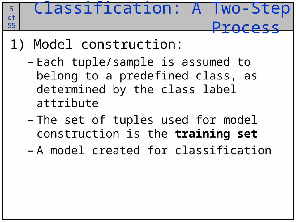
Classification: A Two-Step Process
1) Model construction: – Each tuple/sample is assumed to belong to a
predefined class, as determined by the class label attribute
– The set of tuples used for model construction is the training set
– A model created for classification

6of25
6of55
Classification: A Two-Step Process (cont…)
2) Model usage:– Estimate accuracy of the model
• All members of an independent test-set is tested using the model built
• The known label of test sample is compared with the classified result from the model
• Accuracy rate is the percentage of test set samples that are correctly classified by the model
– If the accuracy is acceptable, the model is used to classify data tuples whose class labels are not known

7of25
7of55
Classification: Model Construction
IF rank = ‘professor’OR years > 6THEN tenured = ‘yes’
NAME RANK YEARS TENUREDMike Assistant Prof 3 noMary Assistant Prof 7 yesBill Professor 2 yesJim Associate Prof 7 yesDave Assistant Prof 6 noAnne Associate Prof 3 no
Training Set
Classification Model
Classification Algorithm

8of25
8of55
Classification: Using The Model In Prediction
(Jeff, Professor, 4)
Tenured?
Testing Set
Classifier
Unseen Data
Yes
NAME RANK YEARS TENUREDTom Assistant Prof 2 noMerlisa Associate Prof 7 noGeorge Professor 5 yesJoseph Assistant Prof 7 yes

9of25
9of55
Supervised Vs. Unsupervised Learning
Supervised learning (classification)– Supervision: The training data (observations,
measurements, etc.) are accompanied by labels indicating the class of the observations
– New data is classified based on the training set
Unsupervised learning (clustering)– The class labels of training data is unknown– Given a set of measurements, observations, etc.
with the aim of establishing the existence of classes or clusters in the data
10of25
10of55
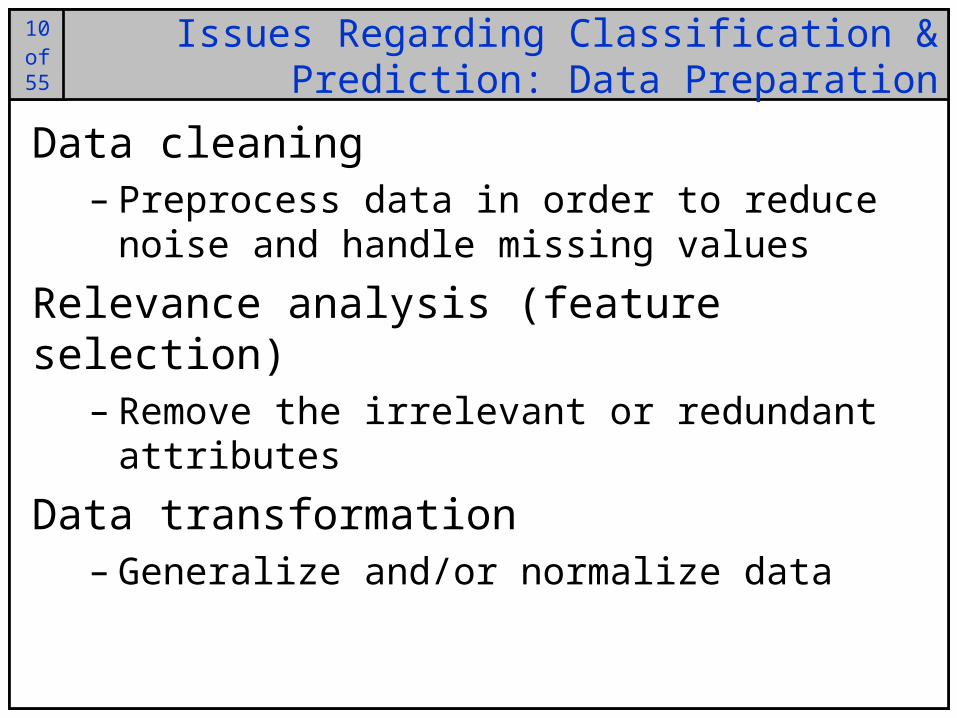
Issues Regarding Classification & Prediction: Data Preparation
Data cleaning– Preprocess data in order to reduce noise and
handle missing values
Relevance analysis (feature selection)– Remove the irrelevant or redundant attributes
Data transformation– Generalize and/or normalize data

11of25
11of55
Issues Regarding Classification & Prediction: Evaluating Classification Methods
Predictive accuracySpeed and scalability
– Time to construct the model– Time to use the model
Robustness– Handling noise and missing values
Scalability– Efficiency in disk-resident databases
Interpretability– Understanding and insight provided by the
model

12of25
12of55
Classification Techniques: Case Based Reasoning (The k-Nearest Neighbor Algorithm)
Case based reasoning is a classification technique which uses prior examples (cases) to determine the classification of unknown cases
The k-nearest neighbour (k-NN) algorithm is the simplest form of case based reasoning

13of25
13of55
The k-Nearest Neighbor Algorithm)
All instances correspond to points in n-D spaceThe nearest neighbours are defined in terms of Euclidean distance (or other appropriate measure)The target value can be discrete or real-valuedFor discrete targets, k-NN returns the most common value among the k training examples nearest to the queryFor real-valued targets, k-NN returns a combination (e.g. average) of the nearest neighbours’ target values

14of25
14of55 Nearest Neighbour Example
Wave Size(ft)
Wave Period(secs)
6 15
1 6
5 11
7 10
6 11
2 1
3 4
6 12
4 2
GoodSurf?
Yes
No
Yes
Yes
Yes
No
No
Yes
No
Class
10 10 ?
Features
Query

15of25
15of55 Nearest Neighbour Example
f1
f2
When a new case is to be classified:
– Calculate the distance from the new case to all training cases
– Put the new case in the same class as its nearest neighbour
?
?
?
Wave Period
Wave S
ize

16of25
16of55 k-Nearest Neighbour Example
f1
f2
What about when it’s too close to call?
Use the k-nearest neighbour technique
– Determine the k nearest neighbours to the query case
– Put the new case into the same class as the majority of its nearest neighbours
Wave Period
Wave S
ize
?
2 neighbours
1 neighbourvs.

17of25
17of55
Nearest Neighbour Distance Measures
Any kind of measurement can be used to calculate the distance between casesThe measurement most suitable will depend on the type of features in the problemEuclidean distance is the most used technique
where n is the number of features, ti is the ith feature of the training case and qi is the ith feature of the query case
n
iii qtd
1
2)(

18of25
18of55
Summary Of Nearest Neighbour Classification
Strengths– No training involved – lazy learning– New data can be added on the fly– Some explanation capabilities– Robust to noisy data by averaging k-nearest
neighbors
Weaknesses– Not the most powerful classification– Slow classification– Curse of dimensionality
One of the easiest machine learning classification techniques to understand

19of25
19of55 Case-Based ReasoningUses lazy evaluation and analysis of similar instancesHowever, instances are not necessarily “points in a Euclidean space”Methodology
– Instances represented by rich symbolic descriptions
– Multiple retrieved cases may be combined– Tight coupling between case retrieval,
knowledge-based reasoning, and problem solving
Lots of active research issues

20of25
20of55
Classification Techniques: Decision Tree Induction
Decision trees are the most widely used classification technique in data mining today
Formulate problems into a tree composed of decision nodes (or branch nodes) and classification nodes (or leaf nodes)
Problem is solved by navigating down the tree until we reach an appropriate leaf node
The tricky bit is building the most efficient and powerful tree
J. Ross Quinlan is a famed researcher in
data mining and decision theory. He has done pioneering work in the area of
decision trees, including inventing the ID3 and C4.5
algorithms.

21of25
21of55 Training Dataset
Age Income Student CreditRating BuysComputer
<=30 high no fair no
<=30 high no excellent no
31 - 40 high no fair yes
>40 medium no fair yes
>40 low yes fair yes
>40 low yes excellent no
31 - 40 low yes excellent yes
<=30 medium no fair no
<=30 low yes fair yes
>40 medium yes fair yes
<=30 medium yes excellent yes
31 - 40 medium no excellent yes
31 - 40 high yes fair yes
>40 medium no excellent no

22of25
22of55 Resultant Decision Tree
Age?
Student?Credit
Rating?Yes
Yes YesNo No
<=30 30 - 40 >40
no yes excellent fair

23of25
23of55
Algorithm For Decision Tree Induction
Basic algorithm (a greedy algorithm)– Tree is constructed in a top-down recursive
divide-and-conquer manner– At the start, all the training examples are at the
root– Attributes are categorical (if continuous-valued,
they are discretized in advance)– Examples are partitioned recursively based on
selected attributes– Test attributes are selected on the basis of a
heuristic or statistical measure (e.g. information gain)

24of25
24of55
Algorithm For Decision Tree Induction
Conditions for stopping partitioning– All samples for a given node belong to the same
class– There are no remaining attributes for further
partitioning – majority voting is employed for classifying the leaf
– There are no samples left

25of25
25of55
The attribute selection mechanism used in ID3 and based on work on information theory by Claude Shannon
If our data is split into classes according to fractions {p1,p2…, pm} then the entropy is
measured as the info required to classify any arbitrary tuple as follows:
iim
pp,...,p,ppEm
i2
1
log)(21
Attribute Selection Measure: Information Gain (ID3/C4.5)

26of25
26of55
The information measure is essentially the same as entropy
At the root node the information is as follows:
94.0
14
5log
14
5
14
9log
14
9
14
5
14
9]5,9[
22
,Einfo
Attribute Selection Measure: Information Gain (ID3/C4.5) (cont…)

27of25
27of55
To measure the information at a particular attribute we measure info for the various splits of that attribute
Attribute Selection Measure: Information Gain (ID3/C4.5) (cont…)

28of25
28of55
At the age attribute the information is as follows:
694.0
5
2log
5
2
5
3log
5
3
14
5
4
0log
4
0
4
4log
4
4
14
4
5
3log
5
3
5
2log
5
2
14
5
2,314
50,4
14
43,2
14
5]2,3[],0,4[],3,2[
22
22
22
infoinfoinfoinfo
Attribute Selection Measure: Information Gain (ID3/C4.5) (cont…)

29of25
29of55
Attribute Selection Measure: Information Gain (ID3/C4.5) (cont…)
In order to determine which attributes we should use at each node we measure the information gained in moving from one node to another and choose the one that gives us the most information
30of25
30of55
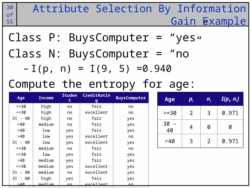
Attribute Selection By Information Gain Example
Class P: BuysComputer = “yes”
Class N: BuysComputer = “no”– I(p, n) = I(9, 5) =0.940
Compute the entropy for age:Age Income Student CreditRating BuysComputer
<=30 high no fair no
<=30 high no excellent no
31 - 40 high no fair yes
>40 medium no fair yes
>40 low yes fair yes
>40 low yes excellent no
31 - 40 low yes excellent yes
<=30 medium no fair no
<=30 low yes fair yes
>40 medium yes fair yes
<=30 medium yes excellent yes
31 - 40 medium no excellent yes
31 - 40 high yes fair yes
>40 medium no excellent no
Age pi ni I(pi, ni)
>=30 2 3 0.971
30 – 40 4 0 0
>40 3 2 0.971

31of25
31of55
Attribute Selection By Information Gain Computation
means “age <=30” has 5 out of 14 samples,
with 2 yes and 3 no. Hence:
Similarly:
694.0
)2,3(14
5)0,4(
14
4)3,2(
14
5)(
IIIageE
048.0)_(
151.0)(
029.0)(
ratingcreditGain
studentGain
incomeGain
246.0)(),()( ageEnpIageGain
)3,2(14
5I

32of25
32of55
Other Attribute Selection Measures
Gini index (CART, IBM IntelligentMiner)– All attributes are assumed continuous-valued– Assume there exist several possible split values
for each attribute– May need other tools, such as clustering, to get
the possible split values– Can be modified for categorical attributes

33of25
33of55
Extracting Classification Rules From Trees
Represent knowledge in the form of IF-THEN rules
One rule is created for each path from root to leaf
Each attribute-value pair along a path forms a conjunction
The leaf node holds the class prediction
Rules are easier for humans to understandIF Age = “<=30” AND Student = “no” THEN BuysComputer = “no”
IF Age = “<=30” AND Student = “yes” THEN BuysComputer = “yes”
IF Age = “31…40” THEN BuysComputer = “yes”
IF Age = “>40” AND CreditRating = “excellent” THEN BuysComputer = “yes”
IF Age = “<=30” AND CreditRating = “fair” THEN BuysComputer = “no”

34of25
34of55 Overfitting
Training Set Test Set

35of25
35of55 Overfitting (cont…)
Training Set Test Set

36of25
36of55
Avoiding Overfitting In Classification
An induced tree may overfit the training data – Too many branches, some may reflect anomalies due to
noise or outliers– Poor accuracy for unseen samples
Two approaches to avoiding overfitting– Prepruning: Halt tree construction early
• Do not split a node if this would result in a measure of the usefullness of the tree falling below a threshold
• Difficult to choose an appropriate threshold
– Postpruning: Remove branches from a “fully grown” tree to give a sequence of progressively pruned trees
• Use a set of data different from the training data to decide which is the “best pruned tree”

37of25
37of55
Approaches To Determine The Final Tree Size
Separate training (2/3) and testing (1/3) sets
Use cross validation, e.g., 10-fold cross validation
Use all the data for training– But apply a statistical test (e.g., chi-square) to
estimate whether expanding or pruning a node may improve the entire distribution
Use minimum description length (MDL) principle
– Halting growth of the tree when the encoding is minimized

38of25
38of55
Enhancements To Basic Decision Tree Induction
Allow for continuous-valued attributes– Dynamically define new discrete-valued
attributes that partition the continuous attribute value into a discrete set of intervals
Handle missing attribute values– Assign the most common value of the attribute– Assign probability to each of the possible values
Attribute construction– Create new attributes based on existing ones
that are sparsely represented– This reduces fragmentation, repetition, and
replication

39of25
39of55
Classification In Large Databases
Classification - a classical problem extensively studied by statisticians and machine learning researchers
Scalability: Classifying data sets with millions of examples and hundreds of attributes with reasonable speed
Why decision tree induction in data mining?– Relatively faster learning speed (than other classification
methods)– Convertible to simple and easy to understand
classification rules– Can use SQL queries for accessing databases– Comparable classification accuracy with other methods

40of25
40of55
Data Cube-Based Decision-Tree Induction
Integration of generalization with decision-tree induction
Classification at primitive concept levels– E.g., precise temperature, humidity, outlook, etc.– Low-level concepts, scattered classes, bushy
classification-trees– Semantic interpretation problems
Cube-based multi-level classification– Relevance analysis at multi-levels– Information-gain analysis with dimension + level

41of25
41of55
Decision Tree In SAS
42of25
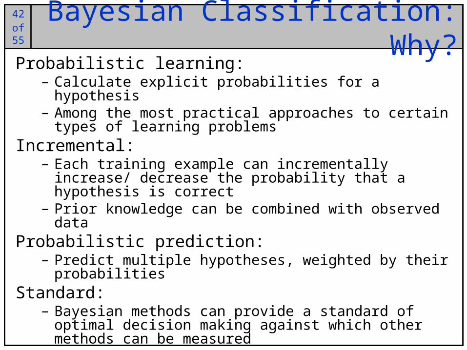
42of55 Bayesian Classification: Why?Probabilistic learning:
– Calculate explicit probabilities for a hypothesis– Among the most practical approaches to certain types of
learning problemsIncremental:
– Each training example can incrementally increase/ decrease the probability that a hypothesis is correct
– Prior knowledge can be combined with observed dataProbabilistic prediction:
– Predict multiple hypotheses, weighted by their probabilities
Standard: – Bayesian methods can provide a standard of optimal
decision making against which other methods can be measured

43of25
43of55 Bayesian Theorem: BasicsLet X be a data sample whose class label is unknown
Let H be a hypothesis that X belongs to class C
For classification problems, determine P(H|X): the probability that the hypothesis holds given the observed data sample X
– P(H): prior probability of hypothesis H (i.e. the initial probability before we observe any data, reflects the background knowledge)
– P(X): probability that sample data is observed
– P(X|H): probability of observing the sample X, given that the hypothesis holds

44of25
44of55 Bayesian TheoremGiven training data X, posteriori probability of a hypothesis H, P(H|X) follows the Bayes theorem
Informally, this can be written as
MAP (maximum posteriori) hypothesis
Practical difficulty: require initial knowledge of many probabilities, significant computational cost
)()()|()|(
XPHPHXPXHP
.)()|(maxarg)|(maxarg hPhDPHh
DhPHhMAP
h
posterior = (likelihood * prior) / evidence

45of25
45of55 Naïve Bayes Classifier A simplified assumption: attributes are conditionally independent:
The product of occurrence of say 2 elements x1 and x2, given the current class is C, is the product of the probabilities of each element taken separately, given the same class P([y1,y2],C) = P(y1,C) * P(y2,C)No dependence relation between attributes Greatly reduces the computation cost, only count the class distribution.
Once the probability P(X|Ci) is known, assign X to the class with maximum P(X|Ci)*P(Ci)
n
kCixkPCiXP
1)|()|(

46of25
46of55 Training dataset
age income student credit_rating buys_computer<=30 high no fair no<=30 high no excellent no30…40 high no fair yes>40 medium no fair yes>40 low yes fair yes>40 low yes excellent no31…40 low yes excellent yes<=30 medium no fair no<=30 low yes fair yes>40 medium yes fair yes<=30 medium yes excellent yes31…40 medium no excellent yes31…40 high yes fair yes>40 medium no excellent no
Class:C1:buys_computer=‘yes’C2:buys_computer=‘no’
Data sample X =(age<=30,Income=medium,Student=yesCredit_rating=Fair)

47of25
47of55
Naïve Bayesian Classifier: ExampleCompute P(X/Ci) for each class
P(age=“<30” | buys_computer=“yes”) = 2/9=0.222 P(age=“<30” | buys_computer=“no”) = 3/5 =0.6 P(income=“medium” | buys_computer=“yes”)= 4/9 =0.444 P(income=“medium” | buys_computer=“no”) = 2/5 = 0.4 P(student=“yes” | buys_computer=“yes)= 6/9 =0.667 P(student=“yes” | buys_computer=“no”)= 1/5=0.2 P(credit_rating=“fair” | buys_computer=“yes”)=6/9=0.667 P(credit_rating=“fair” | buys_computer=“no”)=2/5=0.4
X=(age<=30 ,income =medium, student=yes,credit_rating=fair)
P(X|Ci) : P(X|buys_computer=“yes”)= 0.222 x 0.444 x 0.667 x 0.0.667 =0.044 P(X|buys_computer=“no”)= 0.6 x 0.4 x 0.2 x 0.4 =0.019P(X|Ci)*P(Ci ) : P(X|buys_computer=“yes”) * P(buys_computer=“yes”)=0.028
P(X|buys_computer=“no”) * P(buys_computer=“no”)=0.007
X belongs to class “buys_computer=yes”

48of25
48of55
Naïve Bayesian Classifier: Comments
Advantages : – Easy to implement – Good results obtained in most of the cases
Disadvantages– Assumption: class conditional independence , therefore
loss of accuracy– Practically, dependencies exist among variables – E.g., hospitals: patients: Profile: age, family history etc – Symptoms: fever, cough etc., Disease: lung cancer,
diabetes etc – Dependencies among these cannot be modeled by
Naïve Bayesian Classifier
How to deal with these dependencies?– Bayesian Belief Networks

49of25
49of55 Bayesian NetworksBayesian belief network allows a subset of the variables conditionally independent
A graphical model of causal relationships– Represents dependency among the variables – Gives a specification of joint probability
distribution
X Y
ZP
•Nodes: random variables•Links: dependency•X,Y are the parents of Z, and Y is
the parent of P•No dependency between Z and P•Has no loops or cycles

50of25
50of55
Bayesian Belief Network: An Example
FamilyHistory
LungCancer
PositiveXRay
Smoker
Emphysema
Dyspnea
LC
~LC
(FH, S) (FH, ~S) (~FH, S) (~FH, ~S)
0.8
0.2
0.5
0.5
0.7
0.3
0.1
0.9
Bayesian Belief Networks
The conditional probability table for the variable LungCancer:Shows the conditional probability for each possible combination of its parents
n
iZParents iziPznzP
1))(|(),...,1(

51of25
51of55 Learning Bayesian NetworksSeveral cases
– Given both the network structure and all variables observable: learn only the CPTs
– Network structure known, some hidden variables: method of gradient descent, analogous to neural network learning
– Network structure unknown, all variables observable: search through the model space to reconstruct graph topology
– Unknown structure, all hidden variables: no good algorithms known for this purpose
D. Heckerman, Bayesian networks for data mining

52of25
52of55 Lazy Vs. Eager LearningLazy learning:
– Case based reasoning
Eager learning:– Decision-tree and Bayesian classification
Key differences:– Lazy method may consider query instance when
deciding how to generalize beyond the training data D
– Eager method cannot since they have already chosen global approximation when seeing the query

53of25
53of55 Lazy Vs. Eager LearningEfficiency:
– Lazy, less time training but more time predicting
Accuracy:– Lazy method effectively uses a richer hypothesis
space since it uses many local linear functions to form its implicit global approximation to the target function
– Eager learners must commit to a single hypothesis that covers the entire instance space
– Easier for lazy learners to cope with concept drift

54of25
54of55 SummaryClassification is an extensively studied problem
Classification is probably one of the most widely used data mining techniques with a lot of extensions
Classification techniques can be categorized as either lazy or eager
Scalability is still an important issue for database applications: thus combining classification with database techniques should be a promising topic
Research directions: classification of non-relational data, e.g., text, spatial, multimedia, etc. classification of skewed data sets

55of25
55of55 Questions?
?


