55
By Hui Bian Office for Faculty Excellence 1

By Hui Bian
Office for Faculty Excellence
1

Email: [email protected]
Phone: 328-5428
Location: 2307 Old Cafeteria Complex (east campus)
Website: http://www.ecu.edu/cs-acad/ofe/index.cfm
2

Structure analyzing procedures
Identify the interrelationships am0ng a large set of observed variables.
Use data reduction to group a smaller number of variables into factors that have common characteristics.
3

Exploratory factor analysis (EFA)
Researchers do not know how many factors explain the interrelationships among a set of items.
Using EFA to explore the underlying dimensions of the construct of interest.
Confirmatory factor analysis (CFA)
Researchers do know how many factors explain the interrelationships among a set of items.
Using CFA to determine how well the hypothesized theoretical structure fits the data.
4
Factor analysis uses Person product moment correlations.
The data should have a bivariate normal distribution for each pair of variables.
Observations should be independent.
5

Factor Analysis is primarily used for data reduction or structure detection.
The purpose of data reduction is to remove redundant (highly correlated) variables from the data file, perhaps replacing the entire data file with a smaller number of uncorrelated variables.
The purpose of structure detection is to examine the underlying (or latent) relationships between the variables.
6

No golden rules
10-15 subjects/variable
At least 300 cases
500 (very good) -1000 or more (excellent)
7

The variables should be quantitative at the interval or ratio level.
Categorical data are not suitable for factor analysis.
Data for which Pearson correlation coefficients can sensibly be calculated should be suitable for factor analysis.
If you think the relationships between your variables are nonlinear, the bivariate correlations procedure offers correlation coefficients that are more appropriate for nonlinear associations.
If your analysis variables are not scale variables, you can try hierarchical cluster analysis on the variables as an alternative to factor analysis for structure detection.
8

Step 1 • Specifying problem
Step 2 • Generating items, initially testing the instrument
Step 3 • Assessing the adequacy of the correlation matrix
Step 4 • Extracting the initial factors
Step 5 • Rotating the factors
Step 6 • Refining the solution
Step 7 • Interpreting findings
Step 8 • Reporting and replicating the results
9 Pett, Lackey, & Sullivan (2003)
Principal component analysis (PCA) for data reduction It begins by finding a linear combination of variables (a component)
that accounts for as much variation in the original variables as possible.
then finds another component that accounts for as much of the remaining variation as possible and is uncorrelated with the previous component, continuing in this way until there are as many components as original variables.
A few components will account for most of the variation, and these components can be used to replace the original variables. This method is most often used to reduce the number of variables in the data file.
Hypothetical factors are generated from total variance (the sum of the variances for the original variables).
10

Principal axis factoring (PAF) for structure detection With the assumption that some of the variability in the data cannot be
explained by the components (usually called factors in other extraction methods).
The hypothetical factors are generated from common variance (variance that one item shares with other items), not total variance.
The total variance explained by the solution is smaller; But it is ideal for examining relationships between the variables.
11

Start with a PCA solution
Compare results with a PAF solution
Pick the one that best fits and makes sense
With any extraction method, the two questions that a good solution should try to answer are "How many components (factors) are needed to represent the variables?" and "What do these components represent?"
12

Communalities: total amount of variance in each item that is explained by the factors.
Eigenvalues: amount of variance in all of the items that can be explained by a given principal component or factor.
13

Scree plot
14
Three principal components
Draw a straight line through smaller eigenvalues

Orthogonal rotations
Assumption: the factors are independent of each other or uncorrelated.
Three major approaches to orthogonal rotation: Varimax, Quartimax, Equamax
Oblique rotations Assumption: the factors are correlated.
Types of oblique rotations: Direct Oblimin and Promax
15

Eigenvalue > 1
Percent of variance extracted: cumulative percentage of variance
Scree plot
Factor interpretability and usefulness
16

Example: use EFA to determine the underlying structure in self-image.
30 items for self-image scale
Q59_1 to Q59_30
17

Analyze > Dimension Reduction > Factor...
Enter all self-image items into Variables
Click Descriptive
18

19
Descriptives Check KMO… and Anti-image
Extraction
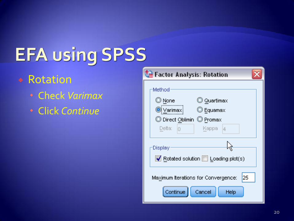
Rotation
Check Varimax
Click Continue
20

KMO and Bartlett’s test: indicate the suitability of your data for structure detection. Kaiser-Meyer-Olkin Measure of Sampling Adequacy indicates the
proportion of variance in your variables that might be caused by underlying factors.
21
High values (close to 1.0) generally indicate that a factor analysis may be useful with your data. If the value is less than 0.50, the results of the factor analysis probably won't be very useful.
Size of KMO Above .90 is “marvelous” In the .80s is “meritorious” In the .70s is just “middling” Less than .60s is “unacceptable”

Bartlett's test of sphericity tests the hypothesis that your correlation matrix is an identity matrix (there is no relationship among the item), which would indicate that your variables are unrelated and therefore unsuitable for structure detection.
22
Small values (less than 0.05) of the significance level indicate that a factor analysis may be useful with your data.

Measures of sampling adequacy (MSA)
Anti-image correlation matrix: indicates how strongly one item is correlated with other items in the matrix. Cut-off is >.70.
23

According to Bartlett’s test (p< .05), the correlation matrix is not an identity matrix.
KMO statistic suggests that we have a sufficient sample size relative to the number of items in our scale.
The MSA statistics indicate that the correlations among the individual items are strong enough to suggest that the correlation matrix is factorable.
24

Communalities indicate the amount of variance in each item that is accounted for by components (8 components).
25
High communality indicates that the extracted components represent the variables well. If any communalities are very low in a principal components extraction, you may need to extract another component.

Eigenvalue
26
1. Total The Total column gives the eigenvalue, or amount of variance in the original variables accounted for by each component. 2. The % of Variance column gives the ratio, expressed as a percentage, of the variance accounted for by each component to the total variance in all of the variables. 3. The Cumulative % column gives the percentage of variance accounted for by the first n components. For example, the cumulative percentage for the second component is the sum of the percentage of variance for the first and second components. For the initial solution, there are as many components as variables, and in a correlations analysis, the sum
of the eigenvalues equals the number of components. You have requested that eigenvalues greater than 1 be extracted, so the first 8 principal components form the extracted solution.
8 factors’ eigenvalues > 1
Initial solution

Eight extracted components explain nearly 66% of the variability in the original 30 variables.
27
The variation is now spread more evenly over the components. The large changes in the individual totals suggest that the rotated component matrix will be easier to interpret than the unrotated matrix.
After rotation Extracted solution

28
The scree plot helps you to determine the optimal number of components. The eigenvalue of each component in the initial solution is plotted. Generally, you want to extract the components on the steep slope. But for this scree plot, I want to extract 3 factors.

Rerun factor analysis using 3-factor solution
Analyze > Dimension Reduction > Factor...
Click Extraction
29
Under Extract Check Fixed number of factors and type 3

42.49% of the variance in the 30 items is explained by 3 components.
30

Rotated component matrix
The rotated component matrix helps you to determine what the components represent.
31
Double loadings

In an orthogonal rotation: such as Varimax
.45: fair
.55: good
.63: very good
.71: excellent
32
Examine rotated factor matrices for high or low loadings
In an orthogonal rotation, factor pattern and factor structure matrix are identical.
In an oblique rotation, those matrices are different.
First focus on structure matrix for factor interpretability and then compare your decisions with loadings in the factor pattern matrix
33

34
Table 1. Factor Loadings from Varimax Rotation for Self-Image Scale of High School Sample
Self-Image Items Factor 1 Factor 2 Factor 3
1. External appearance
Fit/in shape .64
Healthy .54
Having a nice body/figure .71
Athletic .68
In style .70
Cool .66
Good looking/attractive .66
Popular .73
Strong .45
2. Internal characteristics
Responsible .59
Motivated .50
A hard worker .51
Mature .54
Successful .45
Honest/truthful .57
Disciplined .53
Nice/friendly .70
Kind/good .76
Considerate .71
3. Drug using
A pot user .74
Taking drugs .80
A cigarettes smoker .65
A partier .69
Wild .65
An alcohol drinker .78

The same example but using oblique rotation
Analyze > Dimension Reduction > Factor...
Enter all self-image items into Variables
Click Rotation
Choose Direct Oblimin
35
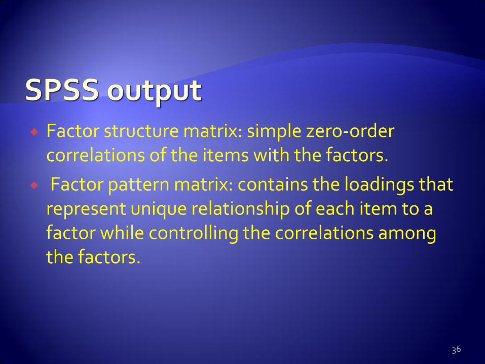
Factor structure matrix: simple zero-order correlations of the items with the factors.
Factor pattern matrix: contains the loadings that represent unique relationship of each item to a factor while controlling the correlations among the factors.
36

Factor structure matrix
37

Factor pattern matrix
38

Correlations among factors
39

Items with weak loadings
Are those loadings <.30
Drop items that do not load reasonably on any factor
Evaluate the weak loading item’s communality and its unique contribution to the instrument
Low communality and little importance to the instrument, the item should be removed.
Important contributor to the instrument, the item should not be eliminated.
40

Items with double loadings
Placing item with the factor that it is most closely related to conceptually.
Based on factor’s internal consistency.
41

We use the same example
30-item self-image scale (Q59)
We want to know the underlying structure of self-image scale
42

The same procedure
Analyze > Dimension Reduction > Factor...
Enter all self-image items into Variables
Click Extraction
Choose PAF
43

Sampling adequacy
44

Communalities
45
PAF PCA
PCA assumes that all of the variance in an item can be explained by the extracted factors. PCA’s initial estimate of the communality is 1.00. PAF’s initial communalities are the amount of variance in one item that is explained by the remaining items and not equal to 1.

46
PAF PCA
After extraction, the amount of explained variance is lower in PAF (55.24%) than in PCA (65.80%), reflecting PAF’s emphasis on shared variance rather than total variance.

47
From 65.80% of initial solution to 55.24% of extracted solution, about 10% of the variation explained by the initial solution is lost due to latent factors unique to the original variables and variability that simply cannot be explained by the factor model.

Scree plot
48
Supports 3-factor solution
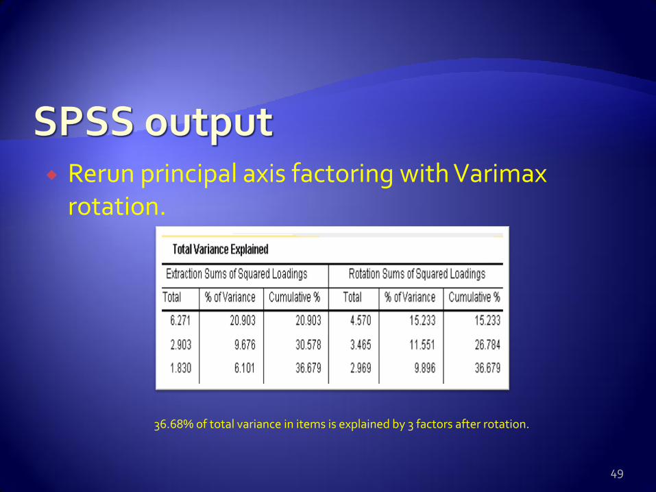
Rerun principal axis factoring with Varimax rotation.
49
36.68% of total variance in items is explained by 3 factors after rotation.

Rotated factor matrix
50

Factor scores: Click Scores
Internal consistency of factors
51

52 Pett, Lackey, & Sullivan (2003)
53

Meyers, L. S., Gamst, G., & Guarino, A. J. (2006). Applied multivariate research: design and interpretation. Thousand Oaks, CA: Sage Publications, Inc.
Pett, M. A., Lackey, N. R.,& Sullivan, J. J. (2003). Making sense of factor analysis: the use of factor analysis for instrument development in health care research. Thousand Oaks, CA: Sage Publications, Inc.
Stevens, J. P. (2002). Applied multivariate statistics for the social sciences (4th ed.). Mahwah, NJ: Lawrence Erlbaum Associates, Inc.
54

55


