A DEFLECTION VARIABL1?, TECHNIQUE FOR THE OPTIMTSATION
OF FIBRE—REINFORCED COMPOSITE STRUCTURES
by
J J . Mc KE OWN
Li. In
A thesis submitted for the degree of Doctor of Philosophy in
the Faculty of Engineering, University of London, March 1977.
ACKNOWLEDGEMENT
I gratefully acknowledge the help and support of the following
in the production of this thesis.
My wife, Deirdre, for her encouragement and understanding on
those occasions when family concerns had to take second place
to the demands of research. Mr. Frank Matthews, my supervisor
in the Department of Aeronautics at Imperial College, for his
advice and encouragement. My colleagues at the Numerical
Optimisation Centre: Mr. S.E. Hersom, Dr. L.C.W. Dixon,
Dr. M.C. Bartholomew-Biggs, Dr. J. Gomulka - all of whom
contributed useful advice as well as acting as 'sounding
boards' - and Mrs. Mary Hunter, who typed most of the
manuscript. Hertfordshire County Council, who sponsored me,
and finally the Computer Centre at Hatfield Polytechnic, who
provided computing facilities.
SUMMARY
This thesis is concerned with the optimisation of multilaminar
composite sheets. The introductory chapter defines the problem
and discusses briefly the main difficulties it entails. The
problem is set in perspective by a brief background discussion
of the related but simpler isotropic one,together with some of
the methods currently available for its solution. A new formulation
is proposed which involves defining the nodal deflections of •
the structure as the primary optimisation variables;the name
'Deflection-Space Formulation' is adopted for this approach.
It is shown in Chapter 2 that the problem is
decomposed into an outer subproblem,in the space of the deflections,
and an inner one in terms of the original design variables. The
latter problem is that of finding the structure of minimum volume
for a given deflection;it is shown to be a Linear Programming
one in an infinite number of variables. This form allows useful
insights to be gained into the characteristics of optimal
structures. An algorithm,named the Tunctional Linear Programming'
algorithm(FIP) is proposed for the solution of the fixed-
deflection subproblem and some numerical results given.
Chapter 3 is devoted to the further development of the FI.P
algorithm and to an analysis of the designs produced by it.
In chapter 4 the properties of the objective
function of the outer subproblem are investigated,and the problem
of designing maximum-stiffness structures is expressed in deflection-
variable form. An algorithm is proposed for designing such
structures and numerical results are presented.
The basic deflection-space formulation is
extended in chapter 5 to include multiple alternative load cases
and direct constraints on stresses,and to include lower limits
upon the total thickness of material in any finite element.
Finally,conclusions are drawn and some suggestions made for the
future development of the deflection-space approach and the
Functional Linear Programming algorithm.
TABLE OF CONTENTS
CHAPTER 1
1.1: Introduction to the problem 1
1.2: Mathematical statement of the problem 4
1.3: The application of numerical optimisation
techniques to structural synthesis 11
1.4: A new formulation 22
CHAPTER 2
2.1: The deflection-space formulation 27
2.2: Implications of the deflection-space
formulation 31
2.3: The deflection-space formulation applied
to fibre-reinforced structures 36
2.4: The Functional Linear Programming algorithm 63
2.5: Numerical results 83
CHAPTER 3
3.1: Introduction 96
3.2: The test programs 96
3.3: Analysis of optimal designs 99
3.4: Performance of theFLP algorithm 142
3.5: Factors affecting the convergence of the
FLP algorithm 149
3.6: Theoretical convergence of the FLP algorithm 166
3.7: Conclusion 168
-iv-
CHAPTER 4
4.1: Introduction 170
4.2: The analogous pin-jointed structure 171
4.3: The dual FLP problem 180
4.4: Properties of the function0) 191
4.5: The maximum-stiffness problem 201
4.6: An algorithm for finding maximum-
stiffness structures 206
4.7: Numerical results 213
CHAPTER 5
5.1: Stress constraints 250
5.2: Multiple load cases 254
5.3: Avoidance of empty elements 256
5.4: The general problem 258
5.5: Summary and conclusions 261
Reference List 269
AMEDIcn-
2.1: The Functional Linear Programming algorithm
2.2: The One-dimensional minimisation routine
• 3.1: Element stress and stiffness routine
3.2: Routine to compute deflections
274
284
289
297
-v-
4.1: Routine to compute derivatives of W(€) 303
4.2: The linear search routine 307
4.3: Implementation of the maximum-stiffness algorithm 312
4.4: Two additional papers 317
-vi-
LIST OF TABLES
Chapter 2 Page
2.1: Simplex Tableau 43
2.2: Functional Simplex Tableau 54
2.3: FLP on Single-Node Truss,Iteration 1 58
2.4: 1/ 2 59
2.5: 11 Final Tableau 60
2.6: Material Properties 83
2.7: Single Element model: Loads and Deflections 85
2.8: Final Design 86
2.9: 4-Element Model: Loads and Final Deflections PR
2.10: Initial and Final Designs 89
2.11: 16-Element Model,Initial and Final Designs 90a
2.12: 32-Element Model,Initial and Final Designs 92
2.13: Comparison of Initial and Final Volumes,
Various Meshes 94
Chapter 3
3.1: 32-Element Model: Initial and Final Designs 104
3.2: II II It Deflections 105
3.3: 11 11 ,1 Stresses 108
3.4: Cantilever Problem I: Initial and Final Designs 116
3.5: ,1 11 It Stresses 118
3.6: Cantilever Problem II: 1, Designs 123
3.7: 11 tt 11 Stresses 124
3.8: Sheet with Hole: 11 Designs 131
Page
3.9: Sheet with Hole: Initial and Final Stresses
132
3.10: Rate of Convergence,Cantilever Problem II
144
3.11: Sheet with Hole 147
3.12: Number of Iterations Needed,Two Problems 149
3.13: Accelerated Convergence,Sheet with Hole 159
3.14: Analysis of CPU Time 162
3.15: Comparison of Unaccelerated,Accelerated and
'Loose' Convergence Rates 165
Chapter 4
4.1: Base Coordinates,Single Node Truss 172
4.2: Optimal Designs,Various Deflections 174
4.3: Comparison,Computed Derivatives and
Divided Differences 200
4.4: Material Properties 213
4.5: 4-Element Model: Comparison of Final Designs 217
4.6: Deflections 217
4.7: Stress Characteristics of Three Designs in
the Sequence from Starting Point A 218
4.8: Design Sequence A 224
4.9: 225
4.10: Final Designs A and B 227
4.11: Stresses,Final Designs A and B 228
4.12: Comparison, Final Sheet and Trusses 234
4.13: Sheet with Hole: Reduction in Waisting 243
4.14: Final Design and Stresses 246
4.15: I I Sequence of Equal Stress Volumes 247
4.16: Effect of different Allowable Shear Stresses 248
LIST OF FIGURES
CHAPTER 1
Page
5
7
1.1: Typical Element
1.2: Notation for Stresses and Strains
CHAPTER 2
2.1: The Single-Node Truss 50
2.2: Typical Distribution 56
2.3: Final Truss 61
2.4: Typical Distribution XL (0'.) 63
2.5: Typical Basic Set of Distributions 71
2.6: Triangular Sheet Problem 84
2.7: Single Element Model
2.g(a): 4-Element Model 87
(b): 11 " Final Layout 88
2.9: 16-Element Model 90
2.10: 11 11 Final Layout 90
2.11: 32-Element Model 91
2.12: Final Layout 92
CHAPTER 3
3.1: Scheme of Test Programs 97
3.2(a): Cantilever Problem 100
3.3(a): Sheet with Hole Problem 100
3.2(b): Cantilever Model 101
3.3(b): Sheet with Hole Model 102
3.4(a): 32-Element Model,Final Layout 106
3.4(b): II I, ,Final Thicknesses 106
3.5(a): I/ iv ,Initial Values of C 109
3.6(a): II II ,Initial Values of IceLpi 109
3.5(b): II II ,Final Values of C 110
Page
3.6(b): 32-Element Model,Final Values of 104.4 110
3.7(a): Cantilever Problem I,Initial Layout 115
3.7(h): 11 11 Final Layout 115
3.7(c): n 11 Final Thicknesses 117
3.8(a): n 11 Initial Values of C 117
3.8(b): 11 n Final Values of C 119
3.9(a): 11 11 Initial Values of loewl 119
3.9(b): n 11 Final Values of /oll.pl 120
3.10(a):Cantilever Problem II,Initial Layout 125
3.10(b): 11 11 Final Layout 125
3.10(c): 11 11 Final Thicknesses 126
3.11(a): /I 11 Initial Values of C 127
3.11(b): It II Final Values of C 127
3.12(n): It II Initial Values of 1044,/ 128
3.12(b): 1/ n Final Values of)044 128
3.13(a): Sheet with Hole,Initial Layout 133
3.13(b): n " Final Layout 134
3.13(c): /1 " Final Thicknesses 135
3.14(a): II " Initial Values of 1011.p/ 136
3.14(b): 11 " Final Values of iolt..p/ 137
3.15(a): It " Initial values of C 138
3.15(b): 11 " Final Values of C 139
3.16: Graph Showing Convergence on Cantilever II 145
3.17: II II Sheet with Hole 147
3.18: Variation off) and r 154
3.19: Minimum ofp ,Unconstrained 154
3.20: II II Constrained 154
3.21: Sheet with Hole,Accelerated vs.Unaccelerated
Convergence 160
4.1: Single-Node Truss
4.2:
4.3:
4.4:
4.5:
4.6:
-x-
4.13:
CHAPTER 4 Page
172
,Function W(b) 175
Physical Infeasibility 176
W(§.) as Locus of Minima 177
Contours of WOO 179
Plot of Dual Feasible Region,
Horizontal Deflection 185
Sketch of Dual Feasible Region,
Horizontal Deflection 186
Variation in W(b) with Load 187
As 4.8,Complete Set of Bars 188
Plot of Dual Feasible Region,
=1.0, =0.5 189
Sketch of 4.10 190
Flow Chart,Maximum Stiffness
Algorithm
210
Operation of Maximum Stiffness
Algorithm 211
4.7: 11
4.8:
4.9:
4.10:
4.11:
4.12:
4.14: 4-Element Model,Convergence 215
4.15: " Design Sequence 216
4.16: Cantilever Problem,Idealisation 221
4.17: 11 II Convergence 223
4.1R(a): II 11 Final Layout A 229
4.18(b): It 11 II 1, B 229
4.19(a): II It Final Thicknesses A 230
4.19(b): II II to It B 230
4.20: Equivalent Truss 233
Page
4.21: Sheet with Hole, Convergence 236
4.22: II It Sequence of Step-Lengths 237
4.23: II It Sequence of values of 238
4.24: 1, " Free-edge Displacements 240
4.25(a): " it Final Layout 241
4.25(b): " It Final Thicknesses 242
4.26: It n Sketch of Volume Distribution 243
4.27: vt II Final Values of 244
4.28: u ti n ,, C 245
CHAPTER 5
5.1: Minimisation of Reduced Gradient in Presence
of Stress Constraints 254
-1—
Chapter 1
Section 1.1 Introduction to the problem
Perhaps the most exciting recent development in materials
technology, from a structural engineering viewpoint, has been
the introduction of high strength fibre-reinforced composites.
Such materials typically consist of a matrix material, such as
a resin or a metal, in which fibres are imbedded. The function
of the matrix is partly structural and partly to protect the
fibres from surface damage which might reduce their strength.
In principle, of course, such materials are not new;
reinforced concrete, fibreglass and even wood are examples of
materials which conform to some extent to this general description.
Such well-established materials, howeve", have seldom provided
any serious competition for metal alloys in applications where
very high strength-and stiffness-weight ratios were required,
such as aerospace construction. This state of affairs has been
radically altered by the appearance of very high strength fibres
whose strength depends fundamentally on the purity of the material
from which they are made. Because of this purity the strength
can begin to approach the theoretical maximum for the material
involved as determined by its molecular bonds. Undoubtedly the
examples which are of the greatest practical importance at the
present time are boron-on-tungsten (usually simply referred to
as boron) and carbon fibres. These are usually imbedded in an
epoxy or polyester resin. Boron/epoxy composite material, for
example, is available as a pre-impregnated (pre-prep) tape.
This allows very accurate laying up to be done previous to
final curing of the structure; it also means that the relative
volumes of fibre and matrix are not variables of the design
-2—
problem.
Like many innovations which offer obvious advantages over
existing practice, fibre-reinforced materials have turned out to
require considerable development in order to overcome the practical
problems associated with their use.Such problems as brittleness
and fatigue will no doubt be solved in due course, and do not
form any part of the subject matter of this work. However,
structural materials with highly directional properties carry
with them a more fundamental design difficulty which might be
termed an embarrassment of opportunity. This stems from the
need to tailor the material distribution in such a way that the
fibre directions are closely aligned with the directions of
principal stress. If this is done, the resulting structure may
be stronger and stiffer than its steel or titanium equivalent;
if not it may be very much weaker. To illustrate this point,
consider a unidirectional tensile stress field 6 in a composite
material whose fibres make an angle be with the direction of 6 .
The usual strength-of-materials formula gives the shear stress
relative to axes along and transverse to the fibre direction as
(6 sin 260)/2. For values of SO up to five or six degrees,
then, the ratio of induced shear stress to longitudinal stress
is about equal to the misalignment angle in radians. In order
to fully use the ultimate tensile strength of a material whose
shear strength is equal to one tenth of tensile strength (a
fairly typical figure), the fibres must in this case align with
the stress direction to within five degrees at most. A further
drawback is that the ultimate tensile stress transverse to the
fibre direction, which is mainly a property of the matrix material,
in typically very low compared with the ultimate tensile strength
- 3 -
of the fibres. Hhdcock ( 1.1 ) makes the following observation:
'To achieve 25 to 40 per cent weight saving, the types of
structural configurations that have been used for metal structures
must be radically changed. Weight savings of this order cannot
be achieved by mere materials substitution. Full advantage must
be taken of the anisotropic characteristics of the material and
its capability of providing strength and load paths for optimum
load distribution within the structure. This will only be
achieved by designing for the composite material from the outset
of the design process'.
In the same vein, C.W. Rogers ( 1.2 ) says: 'The advent of
composites portends many changes in aircraft design practice.
The designer finds that in addition to a structure, he also has
a material that he can and must design for optimum performance'.
Thus the need to develop techniques for the optimum design
of composite structures seems to be fairly well established. It
happens that the emergence of this need has coincided with
considerable steps forward in the development of tools and
techniques for structural design. The most important new tool
is of course the digital computer; and the two most important
developments in technique are undoubtedly Finite Element methods
of analysis and Numerical Optimization techniques. The availability
of a large-capacity digital computer is a prerequisite for any
practical attempt at synthesising real structures using the two
latter techniques. Fortunately the progress in micro-miniaturisation
and in production techniques is rapidly bringing about a situation
in which even small organisations will beable to afford in-house
computing facilities on a level with those which only large firms
could enjoy a few years ago. It seems unlikely, therefore, that
14.
progress in structural design will be held back by lack of computers;
neither is it likely, given the present state of the art of finite
element analysis, that there will be serious difficulties in
producing realistic mathematical models of the behaviour of
composite systems.
This thesis will describe the results of an investigation
into the problem of applying numerical optimization techniques
to the design problem posed by fibre-reinforced composites. A
new formulation of this problem will he proposed which seeks to
overcome some of the difficulties inherent in the problem. In
addition, algorithms will be surgested for solving the problem
thus formulated; results of numer7:cal experiments into the
performance of these algorithms will also be given.
:vection 1.2 Mathematical Statement of the Problem
The structural design problem which will form the subject of
this work can be defined as follows: A two-dimensional sheet is
loaded and supported in its own plane. It is to be composed of
layers of an orthotropic material; the number of such layers is
not prescribed, and may vary with position on the sheet. At any
point the layers are distinguished from one another by the
orientation of their axes of symmetry. The design problem, then,
is to determine at every point on the sheet the number of layers,
the orientation of axes of symmetry which define them, and their
thicknesses, such that the volume of the sheet is minimal subject
to constraints on stresses and displacements within. Relating
this statement to the properties of fibre-reinforced materials,
it will be seen that each layer would consist of a stack of
-6-
pre-preg tapes, all with their fibres parallel(Fig.1.1). It is assumed
that such tapes are available in sufficiently small thicknesses
that the total thickness of a layer can be Ire;arfled as a continuous
variable. A minor assumption is that the distribution of fibres
within a tape is uniform through its thickness. This ensures
that a bonded stack of n tapes, each of thickness t, is equivalent
to a single tape of thickness nt. Finally, it will be noted that
the problem of the optimum ratio of matrix to fibre volume is
not considered: this choice is prescribed by the known properties
of the tapes from which the sheet is to be made.
Before going on to derive the model which describes the
behaviour of the structure as a whole, it will be useful to
consider the stress-strain relationships of the baSic unidirectional
material from which it will be constructed, and in particular how
the orientation of the fibre axis affects the stiffness referred
to a fixed system of axes. Figure 1.2 shows such a undirectional
material. The suffices L, T refer to axes along and transverse
to the fibre axis respectively. The relationship between stress
and strain referred to these axis is:
rE
r 1
11 /2-E/2. o EL
16-7-
V2.1 Ell &22. 6r
641.7 0 121
6
where II__le E22 = Y
21 E11. Thus the quantities E11, E22,
G12 and
Y12 (or21
) serve to define the stiffness properties of the
material completely. Tsai and Pagano (quoted by Haicock, ref.li)
gave the following relationships for the same quan tities related
to the axes x, y at an angle 0 (between X and L).
Qt, Q12.
6x
---41 Q21
[
Q)-2.
Q61 Q62.
7. 2.,
-8-
(The subscripts on 9 used by Tsai and Pagano are retained although
they conflict with standard notation for a 3 x 3 matrix). The
quantities Q.. are defined in terms of lc and 9 as follows: ij
Q„ = 3 Ul + Uz 4. U3 Cos 2.0 4- U4 Cos 449
Q11 3U 4- U2 - U3 Casio + U4 C. 40
Q.1.4 = Qiz = U1 - Cos 40
Q66 = Ui - U4 Cos 4
C-4/6 = A U3 Sin I& 4* U4 Sin 4-0
= = U3 5ih 26 - 04 4-0
where:
U/ =
Uz =
U3 =
U4
=
oY (Ell 4 11. ÷ .921 912, E21.)
I f
± Is , r
2.tk Y' 412. - k. v/f c.11 1742, 621. ))
ty, - Elz) th 1 (Er, E21 — 6)20 E-17 + 4 /Pg12.)
-.11111'21
For the purposes of the present work the matrix Q in equation
1.2 will be rewritten in an equivalent form which expresses more
conveniently its dependence on 19 :
Q = Q o + CA, 40 + Qi 5L4 49 4- Q3 Cos 2 6 + Q4 S z.n 2B /.3
-9-
where:
3U, + U2. U, - Ut o
0, -- I.J., — kJ, 30.,+1.), o
o 0 U,+ Us:, 4..
Qi
-
04 _(.4.
o
- U4
th
0
0
0
-U4
0 o U4
..-
[
0 o -U4
] U4 - U4 0
U3 0
ck --- 3 [
- U5 0
] 0 0 0
.... o 0 U3 /2. --
Q4 0 0 U3/2.
U3 /2 03 A 0
It remains to consider the form of a typical finite element
stiffness matrix. The total stiffness of the sheet is given by
the equation:
1. 4
Hare a. is a transformation matrix associated with the i'th finite
element; there are Ne
such elements and there are L.1 lavers in '
the i'th. The matrix13 is the stiffness of the j'th layer in
the i'th finite element; its value depends on the geometry of
that element and on the fibre angle e and the layer thickness
t.. It can be computed from the well known formula:
-10-
i lt.: == ott C) ici. aLv .... t., , L , ....
V
where v is the volume of the i, j'th layer; qf i is a vector of
interpolation functions (note that it depends only on the
element geometry and is not specific to the layer itself); and
Qii is the matrix of stress-strain coefficients for the layer
which depends on 0 in the way defined by equation 1.2. Indeed,
substituting 1.3 in 1.5and performing the integration will
result in the following expression:
[.
-k 6 -= ti +0,i, . rk i.. CoS 4 0 i ' Z1,1, Si-n 40 i
4- 4Z3,i, Cos 2O + 44)i, St:" leij 1
1.6
Note that the matrices 13. , r=0,1, ..., 4, are specific to the
finite element and not to the layer; thus they are determined
once the finite element mesh is defined. Thereafter the
stiffness matrix for any layer in an element can be computed
simply by substituting the appropriate values of 0i and t..
The total stiffness matrix for an element composed of Li layers
is therefore:
LI:
• = -1? • *e:' Cos 4.e ee.c. j
J=1 Equation 1.6 is clearly of a form that makes it fairly easy to
compute the effect of altering ti or during the design process.
j
The form is independent of the particular choice of finite element
chosen, although different choices will result in different values
for then . 0. component matrices. Finally, it will be observed
k
thatalthoughiR..islinearinti.,it is highly nonlinear in the
fibre angle 0 ij; this is of course a significant feature from
1.5
the point of view of optimization.
The problem is now sufficiently well defined to be stated
as follows:
5.t. Cs 4 o
ti! > (.)
eL. c J
Li, INTEcex
L z 1,2,
= f,Z. — L i'
5 1,7.,•
• I.
The constraints Cs may he functions of stress nr displacement:
for the moment their form will not be restricted in any way.
Problem 1.1Lis a nonlinear mixed-integer programming one.
In the next section the application of numerical optimization
techniques to such problems will be briefly considered.
Section 1.3 The application of numerical optimization techniques
to structural synthesis
Numerical optimization (or mathematical programming) is
concerned with the numerical solution of problems of the following
form :
F(
.5. t • CZ (X) 0i.=1, z , ...1
Cs (3) 0 1.4.1 ) . • •fri
3: eT ri F,C, E R I
-12-
In this general statement the objective function F and the
constraint functions Ci may be linear or nonlinear.
Although the problem of functional minimization has interested
mathematicians for centuries, the large scale development of
numerical algorithms had to await the development of digital
computers. The first case to receive attention was that in
whichFradC. ire all linear functions; this is of course the
linear programming case first considered by Kontorovich (1939)
and later by Koopmans and Danzig (ref.1.3). The immediate
applicability of the Simplex algorithm to problems in the fields
of economic planning and operational research has led to rapid
developments in linear programming and has helped focus attention
on the more general optimization problem. The result has been
the accumulation of a vast literature on the subject, which is
continually being extended as new applications and theoretical
results are found. Dixon (ref.1.4) gives a concise survey of
the state of the art in 1973; any attempt here to give a
general description of methods available for solving the
problem defined above would only result in a duplication of
such work and would in any case cover material not immediately
relevant to the problem in hand. In addition it would fail to
take account of methods which have been especially developed for
the otructural synthesis problem and do not fall under the heading
of mathematical programming techniques. In order to avoid this
difficulty, the rest of this section will describe available
techniques only as they appear to relate directly to the
structural problem. This approach will also enable the problem
of structural design in fibre reinforced materials to be seen
Ne_
L:: 1
Cs (ti,) 4 0
ti, ?'- 0
-13-
in perspective, particularly in relation to the corresponding
problem for isotropic materials. Finally, in what follows one
further restriction will be respected, namely, that only the problem
of large scale structural synthesis will be considered. In this
context the term 'large scale' has two quite independent meanings,
both of which apply. Firstly, in the sense in which mathematical
programmers normally use it, it means 'having a large number of
constraints and/or variables'; secondly, in the specific context
of structural design, it has a sense which excludes detail
design. Thus, in the field of aerospace structures, the methods
which will be discussed would usually be more suitable for the
design of complete assemblies such as wings or fusela ges than,
say, individual panels. This distinction corresponds to the
normal practice in aerospace design offices, where the general
level of stresses is usually determined using a coarse finite
element mesh and the detail design is completed using these stress
levels as a starting point. In computational terms, the detail
design problem usually has a smaller number of variables
(i.e. is 'small scale' also in the other sense of the term)
but is more nonlinear than the large scale problem and often
involves stability constraints and variables which may only take
discrete values.
The large-scale isotropic problem can be expressed as follows:
1.8(i)
L7. 1, 2. , . . . Ne
• ci,
Problem 1.8 can be compared directly with 1.'31 it can be seen
to he a simpler one. The nonlinear variables 0 have completely
disappeared, as have the integer variables Li. The problem has
therefore been reduced to a great extent both in size and in
complexity. However it remains far from trivial, the reason
being that the constraints, which are once again limits on
stress and deflection, are nonlinear in the thickness variables ti.
The scale of problem 1.8 is perhaps best illustrated by
considering the history of efforts to solve it. Numerical
approaches began to be investigated in the early 1960's, and
the progress made in the decade to 1970 has been well summarised
by Gellatly (ref.1.5). An early algorithm of Gellatly himself
will illustrate both the problem and a typical approach to its
solution (ref.1.6). It was based on the method of feasible
directions due to Zontendijk, and proceeded as follows.
Let tk he some estimate of the solution to 1.8 which
satisfies the constraints, and let dk be a search direction at
that point. That is, the next estimate is to he given by:
E.Pt dk
where oC k is a step length whose value is to be determined. In
Gellatley's algorithm two distinct kinds of search direction are
employed. In the case where tk
is strictly on the interior of
the feasible region, that is, where none of the constraints is
satisfied as an equality, the search direction is determined
solely by the function V. In fact, the search direction is merely
the negative of the gradient of V - a simple steepest descent.
This step therefore exploits the linearity of V. In the case
-15-
C (tk) = 0 for some set Sk
of the indices, consider the following
matrix:
1-4 4k. E. EV V 11 -V Cs (SEs
Hk
consists of columns which are the gradients of the objective
function and the active constraints, evaluated at tk. These
columns can be taken to define a space in which the search
direction is represented as follows:
dk= H ip 1. 9
where /3 is the set of coordinates of dk in the space defined
by k. We now make a step such that the value of the objective
function V remains unaltered, while the values of the critical
constraints are not increased. These requirements can be
expressed as:
1.10
where E El, ...,6„ J and C 0, i = 1,7, ..., Sp,
(The number of active constraints is Sn ). Gellatly assigns the
value 1 to thelE. and, combining 1.9 and 1.10 solves the following
set of linear equations to determine the coordinates of dk:
6 t 1-1' H i< (3 E
Clearly this set of equations is at worst positive semidefinite
rind, if nonsingular, can he solved by a method such as Cholesky
decomposition. However, singularity will occur if any of the
constraint gradients are linearly dependent, and must occur
either if tk
is a solution (since the Kuhn-Tucker conditions then
require that H p = 0) or if Sn > Ne -1
There must therefore
-16-
be safeguards in the computer program to prevent trouble arising
in these circumstances.
Following the computation of dk, the step-length a4 must
then he determined in some way to enable tk+1
to be computed.
The process ends when some criterion such as a Kuhn-Tucker
condition is satisfied or when the step length oe is sufficiently
small.
The algorithm summarised above, which is known as Gellatly's
optimum vector method, may be taken as a fairly typical direct
method of solving the mathematical programming problem 1.8.
Other feasible direction methods exist, notably Zoutendijk's
original one. This differs from Gellatly mainly in the way in
which it selects a search direction when tk is on the boundary
of the feasible region; specifically, it employs a linear
programming approach to optimise the search direction. Again,
there exists another class of direct methods ('direct' because
the constraints are considered as such and not: transformed
previous to solution). This in the class of Gradient Projection
methods, in which the gradient of the function is projected onto
the boundary of the active constraints, followed by a steepest
,lescent step on this boundary. These methods suffer not
surprisingly, from difficulties arising from nonlinearities in
the constraint functions. Since some at least of the constraints
in 1.8 are likely to be nonlinear the method seems to have
little to recommend its use. In fact the problem of 'hemstitching'
(as the process of moving on and off the constraints in short steps
is known) is perhaps one reason why gradient projection methods
have not gained wide popularity in the general field of
mathematical programming. This notwithstanding, Brown and Ang
-17-
(ref.1.7) have reported an application of this algorithm to
structural optimization.
The final large class of direct algorithms which have been
applied to the isotropic structural optimization problem is
that of sequential linear programming. In its simplest form,
an iteration of this consists simply in linearisinr the
constraints at the point tk and then solving the resulting
linear programming problem by standard methods. This approach
has an intuitive appeal in that it allows the very sophisticated
methods which have been developed for the solution of large
linear programming problems to be brought to bear on the non-
linear one. The advantages and disadvantages of this and more
sophisticated methods are discussed by Pope in ref. 1.8; the
sequence of linear programs approach has been used by several
workers. One aspect which is worth noting here is that
Linear Programming is the only area in which methods have been
thoroughly developed for dealing with the integer-variable case.
In addition to the direct method, there is another class
of methods which has attracted interest from structural
optimizers. This consists of methods which involve transforming
the constrained problem into an unconstrained one and then
solving it by successive applications of one of the well known
algorithms for unconstrained minimisation. The earliest forms
of the method consisted in adding functions to the objective
in order to penalise any estimate which was infeasible. One
form which was particularly attractive for the structural
optimization problem was the interior penalty function or
-18-
barrier function. A typical one is:
F E; V- rz - G
V- I
For any value of r this function increases to infinity as the
sequence of estimates tends towards the boundary of the feasible
region from the interior; on the other hand, as r tends to zero
the minimum of F tends towards the minimum of V. The procedure
is therefore to choose a value of r and minimise F as a function
of t, using some feasible starting point. The value of r is then
reduced and a further minimisation carried out, this time using
as a starting point the best point reached on the preceding step,
and so on.
The chief appeal of this approach is perhaps the fact that,
as r is decreased, a sequence of monotonically improving feasible
designsis generated. The sequence can therefore he stopped
wherever economic criteria dictate in the certain knowledge that
some gain will have been made. Another factor nddinr to the
attraction is the apparent simplicity of the approach. Tt is
not surprising, therefore, that the penalty function method has
been applied by a number of workers in the area of structural
optimization; some details are given by Fox in ref. 1.8. It
must be said, however, that the simplicity is not so great as
might appear, since some strategy must he adopted for varying
r and also for determining acceptable convergence both in the
sub-minimisations and in the overall iterative process. In
addition it is a general feature of such methods that the
unconstrained minimisation problems become more ill-conditioned
as r is decreased; see for example Murray, in ref. 1.9.
-19-
Before proceeding to consider alternative approaches which
have been applied to the isotropic problem, it is useful to
quote the following summary, due to Pope and Schmit (ref.1.R),
of the main features of the mathematical programming approach in
general.
(a) It is possible to consider the design of a structural
system rather than the design of individual elements; allowance
can be made where appropriate for quantities such as the weight
of structural connections using, perhaps, statistical information,
(b) The behavioural characteristics of the optimum design need
not be presumed, rather they emerge as a consequence of the
design procedure,
(c) A variety of failure modes in each of several load conditions
may he guarded against,
(d) Restrictions on the design variables arising from fabrication
considerations and limitations of the analysis employed can be
treated,
(e) A wide variety of restrictions on structural behaviour
including stress, displacement, buckling, dynamic and thermal
response can be dealt with,
(f) The approach is not inherently linked to weight minimisation;
that is to nay, objective functions other than structural weight
may he readily employed.
In spite of the flexibility of the mathematical programming
approach, it was found (Gellatly, 1.5) that in practice they had
one serious drawback in practical application to the isotropic
structural problem, namely cost. Computational costs per
iteration depend partly on the cost of evaluating the objective
function and constraints (function evaluations) and partly on
-20-
the 'housekeeping' operations such as the equation-solving
required by the feasible direction algorithm described above.
Indeed, much of the computation involved is concerned with
equation solving, both in the stress analysis and in the house-
keeping. It follows that the amount of computation required per
3 iteration will vary roughly as N
e where Net the number of
finite elements, may be large, of the order of several hundred.
However, in addition to this size-sensitivity of cost per
iteration, it was found that, to quote Gellatly, "The number of
iterations required, and the number of analyses per iterative
stage was found to increase more rapidly with problem size than
had been first assumed On the whole, it began to
appear that economic limits on optimization capabilities based
on numerical search methods were being reached".
This setback caused attention to be turned to another type
of approach which became known as the 'optimality criterion'
approach. Algorithms based on this approach dispense with an
explicitly formulated objective function and instead seek to
satisfy some criterion which is known (or assumed) a priori to
characterise an efficient design. Such methods are closely
related to traditional design practice; for example, one method
attempts to achieve a fully stressed design (that is, every
member fully stressed under at least one loading condition)
and in its simplest form is an adaptation for digital computer
of a standard manual method. The other main optimality criterion
used is that of uniform strain energy density.
-21-
Optimality criterion methods have two main advantages. The
first is their intuitive appeal, which is based on their
traditional background and reinforced by their simplicity. The
second is their high computational efficiency in many cases.
These advantages have led to their widespread use; Gellatly
(ref.1.5) and Kelly, Morris, Bartholomew and Stafford (ref.1.10)
give examples. However, the,:, o.Ovontgges have, in the past,
been bought at the expense of some unreliability due to a
rather shaky mathematical basis. For example, it can be shown
very easily that, given a set of nodes connected by pin-jointed
rods to form a truss or a space frame, the optimum truss for a
single loading condition will, under very general constraints
on stress and deflection, be statically determinate and therefore
fully stressed. However, counterexamples exist (e.g. Cox,Hef. 1.11)
to show that the latter condition need not be associated with
optimality when more than one load case is present, and in
general it is neither necessary nor sufficient for statically
indeterminate structures. Similarly, the uniform strain energy
density criterion is associated with structures of maximum
stiffness, and as such need not always be associated with designs
of minimum weight subject to stress and/or arbitrary deflection
constraints. Gellatly (1.5) includes an example where
oscillation occurred when an optimality criterion method was
applied to the design of a simple cantilever truss. However,
such methods certainly constitute a strong challenge to
mathematical programming as an approach to solving the isotropic
structural problem.
In the past few years the picture presented above of the
state of the art in large scale structural optimization has been
-22-
somewhat altered. The steady development of new mathematical
programming algorithms has resulted in more efficient algorithms
than those available five years ago. For example, the penalty
function approach has been made more viable by the development
of more efficient methods of unconstrained minimisation than the
early variable-metric methods such as Davidon-Fletcher-Powell.
Penalty function methods have themselves been superseded, however,
by new algorithms such as the recursive quadratic programming
algorithm of Biggs (Ref. 1.12). These developments, although
they do not yet seem to have made much impact on structural
optimization, must eventually affect the case for choosing,
between mathematical programming and optimality criterion
techniques. The dichotomy between these two approaches has
already been blurred by work such as that of Parthelomew, Morris,
Kelly and Stafford (described in ref. 1.10) and Templeman (ref.1.13)
who seek to devise methods which have the advantagesof optimality
criterion techninues combined with the rigor of mathem&tical
programming. These developments seem to hold great promise.
Section 1.4 A new formulation
The necessarily brief outline of the state of the art of
isotropic structural optimization given above will have served
to show that problem 1.8 is far from trivial. When we return to
the composite structure problem 1.1-, therefore, it is clear that
it is a formidable one. Whereas the isotropic case has one
thickness variable per finite element, the composite has one per
layer; in addition there is a fibre angle associated with each thickness.
But perhaps the most significant difference between the two is the
-23-
presence of integer variables L. in problem 1.1. It is clear
that little hope can he held out for the solution of this problem
by simple extensions of the methods already applied to isotropic
design; even if the additional nonlinearity and the mixed-integer
form are ignored, the increased size of the problem will itself
exacerbate the difficulties already described. There is
obviously a requirement for a new approach. Before considering
the form which this might take, it is interesting to examine some
attempts to solve 1.7 which have already been made.
Hadcock (in 1.1) and Rogers (in 1.2) describe applications
of Boron-Epoxy in the design of aircraft structures. Hadcock
approached the design problem by restricting the choice of fibre
angle to four - 0o, 90°, - 45°. By applying this restriction
and by making simplifying assumptions it was possible to express
the stiffness and strength of the material as firctions of the
percentage of the fibre volume in each of these tour directions.
Timing this information, design was carried out semi-manually,
using an anisotropic finite element program as a tool to analyse
trial design s. Roger's approach is rather similar; clearly it
cannot he considered an automatic design technique. An optimality
criterion approach has been made by Venkayya et al (ref.1.14).
They begin by restricting the choice of fibre angles in the same
way as Hadcock and Rogers, and in this way they avoid the integer
programming aspect of the problem. The result is a problem
similar to the isotropic one, but with more thickness variables
per finite element. In fact, this approach also avoids the
additional nonlinearity which would be present if the fibre
angles were considered as continuous variables. Thus, by
restricting very considerably the choice of fibre angles it is
-24-
possible to transform the composite problem 1.* into an isotropic
problem like 1.8. Such an inherent restriction, however, is
clearly not desirable (although in particular cases restrictions
might be imposed because of, for example, manufacturing difficulties);
in addition the resulting quasi-isotropic problem is inevitably
much larger than the corresponding isotropic one with the same
number of finite elements.
Problem 1.4 has been expressed in terms of the variables
i i t.,8.and L.. However, the physical problem can be viewed
in terms of two distinct classes of variable:
(a)Designifariablest.,9 ' . L., and j
(b) Behaviour variables 6 (deflections or displacements)
and 6 (stresses). ay.
Here 6 is a vector of size Nd
in the case of a single loading
condition, where Nd is the number of degrees of freedom of the
structure. The stress in a layer is defined by three components, NQ
so the total number of stress variables is equal to
Lrl
The two classes of variables play different traditional roles.
In the analysis problem (in which variables (a) are given) only
the behaviour variables remain to be computed. In the design/
optimization problem, however, the design variables must first
he determined. However, because design normally involves
constraints on behaviour, the behaviour variables must also
be computed. The distinction between the two sets of variables
tILerefore more blurred in the optimization case then in the
analysis one. There is, however, a more fundamental definition
of variables to be made in the optimization context, namely, the
choice of optimization variables. The choice for these has often
-25-
fallen by default on the design variables, perhaps because it is
these variables in which the design must finally he expressed
for fabrication. However, it is by no means obvious that the
design variables are in fact the hest choice of optimization
variables. This is a point which seems to have received relatively
little consideration in the literature. One well known paper in
which it was discussed was that of Reinschmidt et al (ref. 1.15).
They consider a very simple structure and optimise it using simple
transformations of the basic design variables, for example,
reciprocals. They found that the efficiency with which a range
of algorithms solved the problem was significantly affected by
the choice of transformation, and they drew the conclusion that
a transformation should be selected which tends to linearise the
constraints even where this makes the objective function more
nonlinear. Although the problem considered was a very small one,
this recommendation will be borne in mind.
The remaining chapters of this work will he devoted to a
more thoroughgoing change of formulation, namely, to the choice
of t. the displacement vector, as the optimization variable.
some advantages of this approach are immediately apparent; for
example, the constraints will normally be specified as
simple functions of 6 (often nothing more than upper limits 0%0
on the absolute value of some of its elements); and even the
stresses will always be simpler functions of 6 than of the ti
design variables. The difficulties are, however, equally
obvious. To begin with, the very simple linear form of the
objective function of 1.7 will be sacrificed. A more conceptual
difficulty arises from the loss of contact with the physical
-26-
variables of the design. Although any design will, in the absence
of instability, posess a unique deflection under a given load, it
is not true that the same deflection-load pair will serve to define
a structure. It will be necessary therefore to devise a means of
inferring a unique, or near unique, design from a given deflection
and load. An additional source of potential difficulty is that
as a search proceeds in the space of the deflections, regions
may be reached corresponding to deflections for which no design
exists for the given load - for example, the negative energy half-
space.
It is hoped that in the following chapters these potential
difficulties will be shown either to be illusory or, at worst,
tractable. It will be shown, for example, that the problem of
uniquely relating a design to n load-deflection pair can itself
he posed as an optimization problem which it is not difficult to
solve, and which absorbs the integer aspect of problem 1.4. This
imposes a two-level structure on the problem, with an inner and
an outer subproblem. A very useful byproduct of this formulation
will be seen to be the insight which it affords into the nature
of the optimal structure; for example, it becomes immediately
clear that certain very simple upper limits exist upon the
total number of layers in the structure and, independently, upon
the number in any finite element in the optimal structure. These
limits arise solely from the choice of finite element mesh and
are quite independent of the particular constraints on stresses
and/or deflection that may be applied or on the particular linear
function being minimised. Above all, however, it will he shown
that the formulation leads to simple computational techniques for
solving the problem of optimizing multilaminar composites.
-27-
Chapter 2
2.1 The deflection - space formulation
In chapter 1, the problem of optimising fibre-reinforced
structures was introduced, against a background of the current state
of the art of structural optimisation. It was pointed out that the
nature of kl4P materials introduces two main difficulties which are not
present for isotropic materials: namely, an inteFPr variable aspect
associated with the problem of finding optimal numbers of layers in
oncb region of the structure ; and an additional number of variables,
file fibre angles, which are nonlinear in their effect on the constraints.
It is clear that a new formulation of the problem is called for which
directly addresses these difficulties, rather than simply an extension
of orthodox methods developed for isotropic materials. In this and
the following chapters an attempt will be made to develop such a
formulation, together with special algorithms for solving the problem
thw; formulated. The essential change will be that the optimisation
problem is regarded as a search in the space of the deflections of the
structure, rather than one in the 'design' variables directly. In
other words, an optimal deflection pattern will be sought, and the
optimal values of the design variables will be inferred from this.
For this reason the approach will be referred to as the 'Deflection-
Space' formulation.
-28-
The deflection-space formulation, which is not in fact limited
to FIP structures, will be introduced in its simplest form as follows.
Consider the structural optimisation problem:
min V(t) t
s.t. gi( o(t)) L 0, i=1,2 M 2.1
t 'a 0
J=1,2 Ne
Visalinearscalarfunctionoft,adesignvectorin01.is a gi
constraint function. 6 is a deflection vector in Od, and is also a
linear function of t . The structure to he designed is thus linear,
that is, it is constructed of linearly elastic material and in loaded
lightly enough for its geometry to remain significantly constant under
load P for all relevant values of t. For the moment, only one load
net is implied, while a consideration of stress constraints will be
postponed until later. We shall prove a basic Lemma:
UMMA 2.1 A necessary condition that a denirn vector t* shall be a
solution to problem 2.1 is that it is a solution to the following
problem:
min V(t) t
s.t. B(a) t = P P1
t.1 > 0. i=1,2, N
Where B OD is an NdxNematrix whose i'th column is the set of nodal
loads in the i'th element of the structure per unit value of ti, if
the structure is deformed in a way given by the deflection vector
under the load P.
-29-
Proof Let (5* be the deflection of an optimal structure satisfying
2.1. Then in general there will be a set of va]ues of t for which this
deflection will be obtained under the load P. Since gi in 2.1 is a
function of the deflections only, all such design vectors will
correspond to feasible structures. Clearly the optimal value t* will
correspond to the minimum value of V(t) for this range of t. Formally,
L* must solve the following problem:
min V(t) t
s.t. K(t) = P 2.2
t > 0 .
where K is the NdxNd
stiffness matrix of the structure, and depends
only on t. Since the material of the structure is linearly elastic,
the stiffness matrix is related to the design variab]es in the following
way:
Ne K = E t i k 2.3
i=1
where k. is a stiffness matrix per unit thickness which depends only —1
on the geometry of the i'th element. For simplicity, we take ki to be
expressed in terms of the global reference system of the structure,
i.e. to be an NdxNd
(sparse) matrix. Using 2.3, the equality constraints
in 2.2 can be written:
K(t) 6 *
Ne = E ti (ki b *) 13 t p 2.4
i=1
If (5* is known, therefore, Lemma 2.1 is proved as a necessary and
sufficient condition. Viewed as a condition on t, however, it
enables us to say nothing about 5 , and so it is proved as a necessary
condition only.
-30-
For any deflection vector 6, Lemma 2.1 enables us to formulate
the problem of inferring .the necessary values of the design variables t.
It therefore associates a value or set of values of t with every deflection
vector 6 for which a solution to P1 exists, and therefore also associates
with 6 a value of V(t). We can regard these as the values of a function
W(o), and we can then derive a sufficient condition that t shall
satisfy problem 2.1 in terms of this function as follows.
LEMMA 2.2 A necessary and sufficient condition that a design t*
shall be a solution to problem 2.1 is that the deflection vector 6 *
associated with it shall solve the following problem:
min W(45)
P2 s.t. gi(b) 4: 0 i=1,2, M
wherr! W(6) is the optimal value of V(t) in Lemma 2.1 for any
deflection 6.
Proof The Lemma follows from the definition of W(d). Since the
value of this function is the minimum volume of any structure having
deflection 6 under the load P, a minimum of the function within the
feasible region defined by gi( 6) must satisfy problem 2.1.
These Lemmas will prove useful from two points of view. Viewed
as optimality conditions they provide some insight into the nature of
optimal structures in general and FRP structures in particular. But
their main importance in this work is that they provide a means of
decomposing problem 2.1 in such a way that the integer programming
problem becomes trivial, while the subproblems involved can be
simpler in some instances than the corresponding problem in the space
of the design variables. The deflection-space formulation, then, is
simply this: find an algorithm for solving P1 for a general deflection
6; then, using this as a function evaluation routine to compute WM,
-31-
solve P2.
The way in which this overcomes or ernes the difficulties inherent
in more orthodox approaches remains to be described. The development
falls naturally into two parts. First, an algorithm for solving P1
will be proposed in the special case of FRP structures. Then, in
chapter 4, some approaches to the solution of P2 will be discussed and
numerical results given for some maximum-stiffness problems. However,
it must be emphasised that this formulation of the structural optimisation
problem is applicable to a wider class of structures than those
constructed from FRP materials, and before proceeding to discuss the
solution of P1, some general implications of its form as an optimality
condition will be examined.
2.2 Implications of the Deflection-Space Formulation
First, problems P1 and P2 will be extended by considering a general
number of alternative load cases. Problem P.1 then takes the form:
min V(t) t
s.t. g. j 6.(t)) < 0 - 0
i=1,2, M
j=1,2,
2 .5
To derive the form of P1 appropriate to this case, recall problem 2.2,
to which the obvious extension is:
= -pz
PQ
2.6
t> 0 _ -
-32—
Here we have NdxQ constraint equations, but not all are independent
since, by the Virtual Work Theorem, for any design t we have
P.t .(t) . P.
1
t o .(t), —1 — — — — — i,j=1,2, 2.7
—1) Clearly, this provides an additional q(Q conditions which are
2
automatically satisfied for any design vector t, and so this number
of constraint equations can be eliminated from 2.6. If this is done
by eliminating one equation from the set corresponding to the load P2,
two from the set for P3 etc, it becomes clear that if Q > Nd, then only
Nd load cases need be considered; and for Q < Nd, the problem P1 becomes
min V(t) t
1-31 El
B r ' P -2
t - -2
P1
t = P —Q —Q t > 0
Here, P.' is not simply the i'th load vector, but the P.H.S. vector
corresponding to the i'th set of equality constr i(i-1 )alats when ,
^quations have been eliminated from it; Pi in; the corresponding
B - matrix. In extending P2, note that equations 2.7 could be regarded
on a statement that if 61
chosen arbitrarily then only (Nd-1) ire
components of 62 can be no chosen, and no on until only oru component
of the Nd'th deflection vector could be chosen arbitrarily, if Q = Nd
.
We denote such reduced deflection vectors, analogously with the
vectors P'. in P1, as: j1'
6 - 2' ... ' 6 Q. Problem P2 then becomes:
IS•t •
—33—
Min
b 1 , b 2 2 b •••,-,
w(...61 ). 1 Q
s.t . gi(b J ) 0
t > 0
i=1,2 M
j-1,2 P2.
In what follows, the above formulations of P1 and P2 will be
understood, although Q will often be explicitly taken as unity.
Clearly, lemmas 2.1 and 2.2 still apply to the extended forms of
P1 and P2. Consider P1. It is a problem with a linear objective
function, Q Nd -
Q(Q-1) linear equality constraints and Neunknowns.
2
If S 52' '
5Q are known, and if Ne> Q Nd - If , then P1 is
-
a linear programming problem in the standard form. The following
theorem can be stated without further analysis.
Theorem 2.1
Let a structure consist of a number of nodes assumed fixed except
fo,' small deflections under load, connected by a number of elements.
Let both the stiffness and volume of the i'th element be Linear functions
ofa"designvari.ablet.,and let the structure be composed of linearly
elastic material. Let Nd
be the number of degrees of freedom of the
supported structure, and let an optimal structure be one which has
minimum volume and whose deflections satisfy arbitrary constraints
under Q linearly independent alternative load sots. Then the maximum
number of elements necessary in the optimal structure is Q Nd
Q(Q-1) 2 •
Proof
This theorem follows immediately from Lemma 1 by way of the linear
-1) programming nature of P1. Since it has Q Nd Q(Q equality 2
constraints, this is the maximum number of non-zero values of ti in
-34-
any basic solution, and in the optimal solution in particular; see for
example Dantzig, ref. 1.3. It is necessary to add a c:iutiolary note,
because of the possible existence of 'degenerate' solutions to the L.P.
The phenomenon of degeneracy will be discussed it more detail in a
later section. For the moment, it is only necessary to state that it
is possible for a number of equal-optimal solutions to an L.P. to
exist. All such solutions when found by the Simplex algorithm will be
basic solutions and will satisfy the above theorem; but every convex
combination of such solutions will also he optimal but will have more
than the maximum number of elements allowed by Theorem 2.1. Bence,
optimal structures can exist which have more elements than required
by Theorem 2.1, but in every case there will exist -impler structures
of the same volume and having the same deflections under the given loads.
There exists a useful corrolary to Theorem 2.1.
Corollary 1
Let a substructure of any structure be defined ns a subset of the
nodes of a complete structure, together with connecting elements. Let
N ' be the number of degrees of freedom of such a substructure. Then,
if the overall structure is optimal, the maximum number of elements
in '.he substructure is Q Nd' - Q(Q-1)/2 if Q < N
d '' otherwise
Nd '
Proof
Let S' denote th? substructure. .5' can he isolated from the
optimal structure provided its contributions to the nodal loads in
the overall structure are held constant. This implies that S' could
be replaced by any other substructure having the same nodal loads and
deflections; and if such an alternative structure could he found which
was also of less volume, then the overall volume of the structure could
be reduced without violating its constraints. But this would violate
-35-
the initial hypothesis of optimality; iL follows that 8' is optimal
in the sense of P1, i.e. is of minimum volume for riven loads and
deflections. Hence theorem 2.1 applies to it. However, S' can only
be influenced by some subset of the load vectors, spanning a subspace
of dimension Nd
1 . The corollary is therefore proved.
The application of the above theoremtn Mt' structures will 13e
undertaken in a later section; but it is interesting to consider its
implications to other forms of structure. Note that the constraints
for which the theorem holds are very general: it is only necessary
that they be functions of deflections alone, and even this can be
relaxed in the FRP case, as will be shown. Tn the case of a pin-
jointed truss or a ball-jointed frame, this w:)nld include alt direct
constraints on stress and deflection, since stresses in these cases
aro dependent only on deflections. The statical doterminacy of
optimal pin and ball jointed structures ran thus hc provod in a very
r;imple and general way. For, ronsiderinr one lo:.d ,.ase only (Q=1) 1
the maximum number of bars necessary in such an optimal :;! ructure,
by theorem 2.1, is equal to Nd, the available number of equilibrium
equations. Of course, this does not oF itself' prove static determinacy,
since the structure cou]d he a mechanism in some parts (stiff under
the fjven loads) and redundant in others. But the corollary asserts
that no such redundant substructures can exit: hence the optimal bar
structure under any net of direct constraints on deflections is
statically determinate.(};ef. 2.1)
This is a very simple proof, yet
establishes the extremely wide range of constraints for which this
well-known property of bar structures holds.
If we turn to the problem of optimising isotropic sheets, again
under any deflection constraints, it becomes clear that the choice
-36-
of finite element mesh may have a critical effect on the optimal
structure. For, again taking the case Q=1, it is clear that if the
number of finite elements exceeds the number of degrees of freedom,
then void elements,that is, elements of zero thickness, are inevitable
in the optimal structure. Steps would therefore have to be taken to
prevent this in those cases where such a situation would be undesirable.
If this is done by setting a lower limit of toi
on variable ti, the
above theorems and Lemmas continue to hold for the variables (t.-t .). 1 01
This concludes the brief discussion of the general implications
of this unusual way of looking at the structural optimisation. It
has served to chow that, simply by formulating the problem in deflection
space terms, it is possible to gain some insight into the general
nature of a wide class of optimal structures. Note that, although
the analysis so far has been based on the assumption that the constraints
in problem 2.1 are functions of deflection only, the two widely
differing examples used to illustrate theorem ,").1 have shown that such
constraints may he quite general,
may for example include stress constraints. It will be shown that this
in also true, perhaps more surprisingly, for FRP structures.
The deflection-space formulation applied to fibre-reinforced
Structures
In introducirg the deflection-space formnlatiot, it has been shown
that we can replace problem 2.1, which is usually viewed as a problem
in t-space with a linear objective function and, usually, non-convex
constraints, by two sub-problems. The first, which nust be solved
repeatedly, is of linear programming form, while the second has simpler
constraints than 2.1, but a more complex objective furction. While
it has been shown that this formulation provides some useful insights,
-37-
it remains to justify the approach as a means of arriving at optimal
structures. The only obvious advantage so far is tnat neither
subproblem has such cumpiicated constraints as the original problem.
In this section it will be shown that the formulation allows the
integer programming aspect of the FRP problem to be contain?d within
the P1 subproblem, and indeed allows it to be dealt with very easily.
However, in order to introduce the problem, it will be assumed that
a fixed number of layers, each with a known fibre angle, have been
previously assigned to each finite element. For example, the continuous
range of allowable fibre angles might, as an initial simplification, be
replaced by a discrete set evenly distributed in this range. In
addition, only one load case will be considered. Problem P1 can then
be stated as follows:
NL. L Ee t • Min
t1, t2 ,.., t
N e -
2.0)
s.t. E I3 i t = P 1.1
ti .> 0, i=1,2 Ne
Ne is the number of finite elements in the structure.
The vector ti is the vector of thicknesses of the layers in the
i'thfiniteelemerit,andisofdimensionL.,wheroL.is the number
cf layers assigned to that element. Matrix (3', which is of size 4.0
Nd x L.1, is the matrix whose i'th column is the vector of loads per
unit thickness of the j'th layer in the i'th finite element, caused
by some known deflection S . The fibre angles do not appear explicitly
because they have been given values which are absorbed in the B-matrices.
-38-
The actual effect of the fibre angles in given by equation 2.3.
The matrix k1 can be derivd starting with the equation for the
stiffness matrix of a typical layer given by 1.6 (dropping suffices):
k.= t{kio 1 2 3 4 + kiCos 40 + ki Sin 40 + ki Cos 20 4 ki Sin 20} 2.9 -1 - - - - -
Let 0j be the fibre angle assigned to the j'th layer in the i'th
finite element. Then the j'th column of 81 is given by:
ki6 . ki b Cos 4u 4 ki 6 Sin 401 +
k1 6 Cos 201 + ki, Sin 20i
-o-- -1- j -2-- j 2.10
(Note that the kr matrices depend on i only, and not on j because they
are functions of the element geometry alone). Introducing the notation:
P , . = k , we can write the j'th column of 8 in the following form: r r
i + i Cos 40i + 01- Sin 4 0 +0 Cos 2 Oi i Sin 2 0 -o -1
2.11
The vectors P can be computed once for all for a given finite element -r
mesh and deflection vector, and the columnsnf Bi aro then rapidly
calculated by substituting the given values of 0i into 2.11.
Theorem 2.1 can be applied to problem 2.Wito yield the following
results.
(i) The maximum total number of layers necessary in the optimal
structure is equal to Nd
for the Cane Q=1
(ii) The maximum number of layers necessary in any element of the
optimal structure is equal to the number of deformation
modes of that element for Q=1.
Statement (i) follows from the fact that every layer is an element in
the sense of Theorem 2.1; while (ii) follows from the corollary to
that theorem, taking a finite element as a substructure.
-39-
Problem 2.8609 is a standard linear programming problem when the
0, are known, subject only to the proviso that, the Li must be chosen N
sucht.hatEe l,.>.Nd. That is, there must be more variables than
i=1
constraint equations. This condition is easily satisfied in every case.
Of course, there is no guarantee that a solution will exist for any
given deflection ; but this is a point which will be explored in
chapter 4. The methods available for solving a standard Linear
Programming Problem such as 2.4Nare all based on the simplex algorithm
of Dantzig (ref. 1.3). Although this method is extremely well known,
rt brief description of it is included here in order to introduce the
notation, and some of the ideas, which will be used in the next
section to develop a new algorithm to solv? the nonlinear mixed
integar form of. Pl.
The Simplex Algorithm
Consider the general problem:
Min W ctx
x
9.t. B x d
x. 0
i = 1,2, ..., n
where B is an mxn matrix of real numbers, m < n, and d. > 0, 1
i ,1,2, m. An important concept in Linear Programming is that
of 'basic' and'non-basic' variables. Consider an arbitrary division
of the variables into two groups, represented by a vector x1, of
length m, and a vector x2 of length (n-m). The matrix B can always
be correspondingly partitioned into submatrices B1 and B2, where B
1
-4o-
is square; and c into c1 and c
2. The objective function can thus
be written:
lt 1 2t 2 W = c x c x — — — —
and the equality constraints are:
B1x1 + B
2x2
= d
If B1 is non-singular, then:
1-1
x1 = B (d - B
2 x2)
Using 2.13(iii) in 2.13(i) we obtain
2.13(i)
1t
1-1 2 2 W =W1 + (c2 -c B B) x — — — — —
- it
1-1
where W1 = c B d . — — —
2.13(iv)
Clearly, if the values in x2 are chosen arbitrarily, the vectors x1
and x2 will satisfy the constraints 7(ii) so long as x
1 satisfies
2.13(iii).
We will now consider the optimality conditions on x1 and x
2,
hearing in mind that at the solution all the variables mu.-,t have non-
negative values, by 2.12 (iii). First of 911, we introduce the
notation:
lt B
1 c ,
= 2 - c B B-)
the (n-m) vector c' is termed the 'reduced gradient: vector'; it gives
Lhe steepest ascent direction for the function W, if the variables
are always constrained to satisfy 2.13(ii).
Let us now examine the i'th element of x2 at th- solution, together
with the corresponding element of cl'4. Three cases are to be considered.
(i) > 0. Then from 2.13(iv), any decrease in x.2
will further a
reduce W; so, if is optimal, xi must be zero (since no further
decrease in its value is then possible).
I I-
(ii) 1 c14 ' . < 0. Then the solution cannot he optimal, since W
2 can be decreased by increasing x., and this win not violate the
positivityconstraint.If,inincreasingx.2 , we cause one of the
x1
elements to decrease to zero, that element can be exchanged for
x2. The new value of cW . must then be examined.
(iii) c' i = 0. Then, x.2 can be reduced to zero without violating
-W,
2.12(iii). If, in the course of reducing x2
any element of x becomes
zero, then this element of x1
can be interchanged with x.2 as in case (ii).
This reasoning, though not purporting to be an exhaustive proof,
should serve to demonstrate that, at the solution, x2 will be zero;
in other words, a non-basic set of variables, (n-n) in number, can be
found, all of which are zero; and the corresponding reduced gradient
vector c' will have all elements positive or zero. A vector x which
satisfies 2.12(ii) and 2.12(iii) is called a feasible point; if in
addition at least (n-m) of its variables are zero, it in a basic
feasible point. The argument above should show that the solution to
problem 2.12 is a basic feasible point.
:letti.ng x2= 0 in 2.13(iii) yields: -1
x1= B
1 d 2.13(v)
Vit; follows that basic points are generated by choosing m columns from
. B and solving for x1; 3f all the elements of x
1 turn out to he non-
negative, such points are also basic feasible.
The simplex algorithm, devised by Danzig in 1947, se-Ls out to
solve Linear Programming problems by systematically generating basic
feasible solutions of reducing function value. Any such algorithm
must converge, simply because only a finite number of basic feasible
solutions can exist for a given problem, and the requirement that the
.7
-42-
function value must decrease on each iteration means that no such
point can occur more than once. (The case where no r,duction in W
can be made on some particular iteration is called the 'degenerate'
case, and will be touched on later.)
The algorithm begins from a known feasible solution. On each
iteration, the elements of c' are examined. If all are non-negative,
then a solution has been reached. If riot, the non-basic variable
corresponding to the most negative value of 4 is allowed to increase.
If this results in all the elements of x1, as calculated from 2.13(iii),
increasing then the problem is clearly unbounded; no solution to the
problem exists. Usually, however, at least one element of x1 will tend
to decrease as the non-basic variable is increased. The first such
variable actually to become zero is chosen to leave the basic set, and
replace the non-basic variable which is now positive. The result is a
new basic feasible point which has a lower function value. The case
when one of the x1
variables is zero to begin with and decreases
with increasing value of )( is the degenerate case; the iteraA.on
qien results simply in a change in the basic set which usually leads
to a non-degenerate -•Else on subsequent iterations. The Simplex
algorithm is so arranged that the inverse of B1 is continually updated
no that repeated inversion need riot be done; this is of course made
possible by the fact that only one column of B1 is changed on each
itf.rntion.
The actual operations of the algorithm are usually represented
in tableau form. The initial tableau can be generated by arranging
the equation 2.12 in the following form:
J 1 1 1 ! 2 x1
x2 . . . .xm tx 1
1
1 0
0 1
• •1 -c
W 1
xp
n-m
1-1
B B2
' -cW
-0
•
(n-m)
- 0
+1
0
B1 1
d
t- 1 B d 0
-43-
B1
B2 ' 0
x2
W
1t
't 2 k -C-C -11 _ i _ t
0
(Where the objective function has been written -cltx1-c2'x2 +W = 0).
This set of equations is then transformed
1-1 2
I , B B2
1 t -1
0 ' ( -c2t+c
1 B1
B2) ' +1
xl I I Bi -1
d
x 1t 1-1
c B — -1 W
r-
This enables us to write down the initial simplex tableau:
Table 2.1
The variables have been arranged such that the first m constitute x1.
Clearly the last column gives the values of x1
and W. The next step
1-1 is to chose the column from B B
2 corresponding to the most negative
value of '
cW'. this decides which non-basic variable will now enter the
basis. The problem is then to decide which variable should be
replaced in the basic set, i.e. which row of the new basic column should
(B1
d). i.e.isuchthatr.= - -)i
i
-1 = Min Z 0.
-44-
he the pivot element. This is decided by a consideration of ?.13 (iii)
which gives the change in the x1 vector for changes in x as:
, 1-1
2, x1 + 0x1 = B 1
d - (B1 B ).4x2. 1
when the first R.H.S. term is the right-most column of the tableau;
and the second term is the new basic column. Since one of the elements
of x1 is to become zero, and the others are to be non-negative, we
choose i such that:
-1
0 = Min ((B1 d). J
- (B-1B2)1 ), i 1
i=1,2, m
(B1 ") •
(B B)lj 0.
- J J
f 1-1 i The tableau is then pivoted on 03 B -)
PN
The i'th element of x1
then drops out of the basis to he replaced
by x2. and the algorithm proceeds as already descihed. 3
The Following special cases are important -
(i) No initial basic feasible solution known. This is in fact the
usual case in our application. The problem is then solved in two
phases. In the first phase we introduce m new variables:
t Yll Y2' , ••. Ym =
m
Associated with them is an objective function jg = Yi. i=1
The secondary problem is then posed:
m
Minim .g= /2 Yl 1=1
s.t. B x + z = d.
ctx - W = 0.
x. 0, i=1,2, n
y. 0, j=1,2, m.
This is another Linear Program, for which the basic feasible solution
z = d is known. If a solution to the primary problem exists, then A
can he driven to zero; the resulting value of x is clearly a basic
feasible solution for the primary problem. The 'special variables'
2. are then dropped and phase 2, the solution of the primary problem,
cnn proceed. Conversely, if A cannot he reduced to zero, then no
solution to the primary problem exists.
= 0 for one or more values of i on some iteration.
1-1 • If (B B)1 < 0, then no difficulty results; if not we have the
degenerate case already mentioned. In such a case, although the basis
can he changed, no change in the values of the basic variables can be
made without causing one or more of the basic variables to become
negative. Thus the objective function cannot be reduced on that
iteration. The basic convergence proof already stated thus breaks down,
and 'cycling', i.e. generation of a cyclic sequence of solutions is
possible. However, although methods exist to restore theoretical
convergence, these are regarded by most optimisers as unnecessary,
-46-
and in fact no case of cycling has ever been reported in practice
(ref. 1.3). In consequence, the theoretical problem will not be further
considered in this paper, although mention will be made of it in
discussing numerical results.
The Revised Simplex Algorithm
The Simplex algorithm can be greatly improved, particularly in
the case where the B matrix is sparse, if this matrix is not transformed
on every iteration. It will be noticed that on each iteration, only
two parts of the transformed tableau are used. These are:
(i) the last row if the tableau, i.e. the reduced cost c'.
(ii) the column of the transformed B2 corresponding to the most negative
reduced cost.
It is only necessary, therefore, to update B1 -1
on every iteration,
and to use this to compute these quantities. This reduces the amount
of work done on every iteration as compared with the Simplex method
and allows the matrix B to be stored in a compact form, since it is
never actually changed. The updating of B1 -1
is easily accomplished
by noting that the pivoting operation is equivalent to a premultiplication
by the matrix:
1 0 c1 • 1,1 .."
0 1 q 2 i '''' ,
0 ... 1 qm+1,i ]
(B1 2
where, if the_Pth column of (B B2) is denoted by a, the elements
o ---
0 11108 1 qm+1,I, .
i =I
-47-
of a are defined as: qr .
i - a
r/a . . r i
1/a. r
The steps in the revised simplex algorithm are therefore as follows:
Step 1 Form a row vector 71- = etH
Where H is the current inverse basis matrix, B1
and e is the (m+Wth unit vector.
Form c'= c 2 --2
Step 2
Find c'J = Min {c'i}. .
If c'J 0, stop.
Step 3 Form a = H B , where BJ is the J'th column of B - - -J ..._
g= H d
rI = Min {O./a. a.> 0 }.
.
Step 4 Form E = 1 0
0 1
0 0
{
where qiii = - ai/cx, ,
1/aI ,
Update H by forming 111- , E H, net H-e, return to ntep 1.
This is a very basic description of the Revised Simplex algorithm,
which has been greatly improved in recent years. However, most of
the improvements have been concentrated in the area of improving the
updating procedure for H, so as to minimise storage and improve
stability. The logic remains very much as described above. The
-48-
description thus provides a starting-point from which we can proceed
to describe the real problem with which this section is concerned:
namely, the exact solution of the nonlinear mixed integer problem which
P1 becomes when we do not pre-assign values to O. and L.. 1
The full fixed deflection F.R.P. problem is as follows:
Ne
L.
Al1
Min . t
t1 Ne 1
Ne L i=1 j=1
s.t.
Bi ( 0i,L.) ti = P —
i=1
2.8(b)
0 IT Oi. S 7
L. > 0E R L
L. , integer
where 0 is the vector [01, OLd
Comparing this with 2.8(a), the main differences are teat the
constraint-matrix ) instead of being known, is a function of 0 ,
the unknown fibre angles; and that the number of variables is unknown.
Wo thus have the interesting situation that the number of variables
in the problem is itself a variable of the problem. Each column of
i is of the form 2.11, but with 0
i as a variable; B
i is therefore
nonlinear in 01 .
Problem 2.8(b) is evidently much more complex than 2.8(a); it
would seem that the Linear Programming nature of the problem has
vanished with the introduction of the non-linear variables gj, and
the integers :L.. However, the new problem can be regarded as the
-49-
limiting form of the old, when L:—* 00. That is, 2.8(b) can be seen
as a linear program with an infinite number of variables, one for
every value of 0i in the given range. This is the fact which will
be used to develop algorithms for the solution of 2.8(b).
The basic approach is to consider the effect of pre-assigning
values to L and 0i, as in 2.8(a). A systematic form of this would
be to divide the allowable interval of B l, say 0 < 0l it , into
(L.-1) equal intervals and use the end points of such intervals as
the values of 0i for that element. The more intervals chosen, and
thereforethegreaterthevalueofL"the more closely does the
final design approximate to the 'true' optimal design (for the
given re infinite
in the given range. It must be emphasised, however, that no matter
how many layers are assigned to an element to begin with the maximum
number that will remain when the optimal design is found will be
fixed by Theorem 2.1. nie effect of increasing L., therefore, is to
improve the precision with which the solution to 2.8 is found, at the
cost of increasing the number of variables in the linear programming
problem. In the limit, the exact solution would require an infinite
number of variables, corresponding to an infinitely fine division of
each interval on the Oi. The implementation of such an approach
is clearly impracticable, and yet without it it appears impossible
to achieve one of the aims of the new formulation, namely, solving
the integer programming problem involved in determining the optimal
F.R.P. structure. However, it will be shown to be possible to
generalise the Simplex algorithm in such a way as to enable problem
P1 to be solved without the approximation implied by formulation 2.8(.40.
In order to introduce this generalised method, which will be referred
•
-50-
to as Functional Linear Programming, it is convenient to call upon
a very simple structural optimisation problem which is directly
analogous to the F.R.P. problem, and which provides a ample vehicle
for the ideas involved.
The Problem of the Single-Node Truss
Consider the problem depicted in figure 2.1 A structure is
required which will transmit loads P , P from a point A to a number x y
if earth points e1 eN distributed along the straight line E- E.
N a. E
FrgURE 2.1
The elements connecting A to e. are straight pin-jointed bars, and A
must deflect by amounts given by [a x, 6y]. A is unit distance above
E-E, the deflections being insignificant in comparison with this
dimelmion. The length of the i'th element is 1/Sin 0 i, where 0 .
is the angle between the bar and E-E, measured anti- clockwise; and
the contribution to the loads at A made by this element under the
given deflection is easily shown to.be:
-51-
Cos20Sin 0 + Cos 0 Sin2 0 .6 y i x
01 = 1
Cos B .Sint 0 .6 + Sin3 0 Y i x
The fixed-deflection problem for this structure is clearly the
following ordinary linear program:
N
Min 14E: ti/Sin 0 i 1=1
s.t. B t = P
t Z 0
[
where B = p -I
The 2x1 column vectors Pi are of course formed by substituting the
known values 01, 02 ...,0 N into expression 2.15.
Theorem 2.1 immediately gives the maximum number of bars of non-
zero cross section in the optimal structure as two; so long as N z 2,
problem 2.16 is a linear programming problem which, for given
values of 6, can be solved to yield the optimal values of t, the
thicknesses of the bars.
Problem 2.16 can be regarded as an approximation to the continuous
problem obtained when 0. is allowed to take on any value in the
range[OOT] . To see how this problem migh' be solved, note
that, in 2.16, the matrix B could be compactly represented as:
0(0) 4 . That is, the matrix is represented by a single = v1 • • • • °N
vector function, together with a set of values of 0 which, when
substituted into generate the column of E. The vector function
is of course given by:
'Cos20 Sin 0.6 x + Cos 0 Sin20.6 0(0) =
Cos 0 Sint 0.6 x + Sin30.6 y
2.15
2.17
-52-
By using expression 2.17, we can represent the matrix B very
compactly - although in practical comput:itional terms the
compactness of the representation depends on how many constants
must be stored to represent the functions pi(0) which make up
the vector function . Considering for the moment only the
notation, it is necessary to devise a way of representing the
product of h(0) with a vector such as t. This c.11 he done as
follows. Let X(0) relate to t in the same way as the 01 •••
B id
vector function P(0) relates to B, that is, let it represent
the vector: [t t ]. The quantity B t is then representable 1 td
as[P(0), X(0)] A = h , and just as P(0) condenses B to a 1
• • • 09 Td
vector function,X(0) can be thought of as representing t by a
scalar function. If, in the same spirit, the vector
[ 1 1 , is represented as 6(0)
0=a we
J sin°1
sin t9 _1 , ..., ON
can write 2.16 as:
Min W = p(0), x(0)]
x(9) 0
s.t. [(0), X(0)] = p
2.18
X(0) Z 0
(where 0 represents the set el, ..., ord.
a) far, of course, the main improvement of 2.1W over 2.16 is in
compactness of representation; it has taken advantage of the
known functional relationship between the columns of B in 2.16
by introducing 0(9) into the formulation. In doing so, however,
it has added information to the problem statement by explicitly
representing the functional relationship. The problem, however,
equivalent to:
S.t.
/0
yi 0
X(0) z 0
-53-
ntnys the same; the real point is that, as will now be shown,
the simplex algorithm can be applied directly to the compact
representation 2.18.
Consider first the phase 1 problem of finding a basic feasible
solution to problem 2.18. If y1, Y2
are special variables (see
equation 2.14) we can write this problem as:
min
Y, X(9) u"3
s.t. p(0), X(/9)]0 + I P
6(0), X(0)4 w = cl
y. 2 0 , i=1,2
x(0) 0
and, by writing xi, u ta = ut (P - [P(0), X(0).1 ), this is O
L0tP1
The values of X(0) not currently in the basis will he marked X *(0).
This leads to the following initial tableau (table 2.2).
-54-
X'(9) 5'1 Y, VI Azd
Cos20 Sin g 1 0 0 0 1
Sin . 2 9 Cos 0 0 1 0 0 0
-c IW , - 1/Sin 0 0 0 1 0 0
-12 Cos ? "OSin0+Sin20 Cos° 0 0 0 1 1
( 0= 01, ON)
Table 2.2.
To show how the ordinary Simplex algorithm can he applied to this
tableau, the step of the first iteration will he briefly described.
Steps 1 and 2
Find the minimum reduced gradient, that is, examine the last
row of the tableau to find the maximum entry. In this case, during
the first iteration the last row is represented by:
(Cos20 Sin0+Sin20 Cos° ),= n . Hence, one must evaluate 1' . N
thisfunctionforeachofthegivenvaluesofmd choose the
one, say 0j, which gives the maximum value.
Step 3
Form a = P (6p, and A = P
rI = min {a/6. la. > 0} .
Thus, this step is almost exactly the same as for the normal
representation, the only difference being that instead of selecting
the column a from among an explicitly-enumerated set of vectors,
one substitutes the value 0 into the vector function 0(0).
-55-
step 4.
Pivot the tableau on ?,(6y. This is simply a matter of forming
E in-the usual way from the elements of a, and premultiplying the
tableau. This reduces 0(0J ) to a unit vector, and in doing so,
alters the functions representing the columns of the tableau which
are non-basic. The function representing c' (0) is also changed,
and the algorithm can now return to step 1 for the next cycle; one
of the unit vectors is now labelled (0J' tJ Yi ) rather than .
The most obvious advantage of the procedure above is that the
storage requirement is dramatically reduced as compared with an
explicit representation. One must only store P(0), 0(0j), I! and P,
torotherwiththegivensetofvaluesofe9..This reduction in
storage becomes more marked as N increases, that is, as the number
ofallowriblevaluesofe.become greater; for in this case, only the a
vector 0 = 01, ..., O ri needs to be extended. In fact, if 0 is
allowed to take any value, the explicit representation becomes
impossible, while the compact representation is actually reduced in
size, for the vector 0 need no longer be stored. This is the real
value of the compact form, and is the feature which will he exploited
to allow the problem to he solved when no restrictions are placed
on allowable values of 9. except that they must lie in the range 0 tor . The notation used in 2.1P will still apply, with
redefined simply as:
oa le
0 <7 0 1T
note, however, that the quantity [b(0), X(0)] in this case O
represents a finite vector as before, but one which is formed by
the multiplication of a matrix of size (2 x 00) by a vector of
-56..
infinite length, This is the case because x(0) now represents
a vector: [to , to , ...] where there is an element for every 1
point on the interval LOOT] . However, it has already been
pointed out that no matter how many bars are allowed, the largest
number that can occur in any basic feasible snliitinn is, in this
case,two.Hence,atsuchasolution,t0 ,nforevery(9.in the
range 0 except two. Such a situation could he represented by figure 2.2.;
the vertical lines represent the values of t1 and t, at the optimal
bar angles 01 and 0,.
Figure 2.2..
Hence, at the solution, [13(0), X(0)]0
will, in fret, be equal to:
t 0 ( 0 + t0 ( . 1 1 2
However, 01 and 6)2 are not known a priori. The unknown quantity
of the problem can thus he regarded as a distribution, x(0), over
-57-
the set 0 where a distribution, in this nt'rw;v, is defined as a
finitenurriber,inthisc:Isetwo,ofpairsoftimhors(4.,t )
The choice of values of 0. is clearly infinite, although only two
such values are ever actually considered at any one time.
Consider now how the step described for the discrete form of
2.12 are modified when 0 becomes the complete range 0 to r .
Steps 1 and 2
As before, the negative of the reduced cost of the special
function is given by: (Cos20 Sine + Sin 0 Cos0 ). Now, however,
instead of finding the maximum over a given finite sot of values,
we must, evaluate the maximum value of the function for 0 in the
given range, saYE(137T.1
which we will call 0 . min
. The result will yield a value of 9
Steps 3 nnd 4
These are exactly the s-ime an before. We shrili ;,Itrodure the term
'particular column' to refer to 0( 0. ) and, io later iterations, — min
11 0( 0. ). In order to fix ideas, the example nlre:,dy introduced -- min
will he worked through in detail for the case 0 S 0 < 71 . We begin in phase 1, minimisingd.
The Complete Solution to the Truss Problem
Step 1
Minimise the reduced gradient function over 0 (i.e. maximise
-c' (9))
2 2 cos = -(Cos 6 Sine + Sin e Cos 0), o< 6
-58-
Thin will be found to give
c's
0 min )12
The new variable to enter the basis is then X( ).
The corresponding particular column is shown in table 2.3
X" (0) T, q. y1 y? k)/ :3
Cos20 Sing
Singe Con 6 1
2 1 r--- 4 2 1
o
0
0
0
1
0
0
0
0
1
0
0
o
0
1
1
0
0
+1
1 -2- „r.
- I-- .1 2
1
li
Sin 0
(Cos2 C) Sine +Sin2
e ccme)
TAI3LE 2.3 Ste) 2
We now proceed to choose a suitnhle pivot row by examining the
ratio of the first two elements of the right-hand column to those
of the particular column , only positive elements of this
column being considered. The minimum value is 10 and so
2,/ r2
the pivot element is that boxed in the tableau, and y2 is to be
eliminated.
-59-
Step 3
Carrying out this operation, we obtain the following tableau
(table 2.4):
w 17
X *(0 ) Y1 t7 w s
Cos20 Sin 0 -Sin
20 Cos 9 1 0 () 0 1
2,P7 Sin20 c88 9 o 1 0 0 0
1 1 F °Cos() 0 0 1 0 0 - Sin Sin 0 +
-Sin-0 Cos 0+ Cos29 Sint) 0 0 0 1 1
Table 2.4
One of the special variables has thus been eliminated, and the
variable t introduced, with its corresponding parameter-value of 1 .
Note that the general column, and its associated cost functions,
have been transformed in the process. The new cost function for,i
is:
c' = -con29 sin 9 + sin -0 cos()
and repenting Step 2, we have
1 3.-rr CI8 - = v =
nun 2
-60-
The new particular column is therefore:
-1
_2,17
Again, the pivot element is boxed. Special variable y1 is thus to
he eliminated and renlaced by a particu]ar vnri!)1)10, t , corresponding
to 0 = . If this is done, (Step 3 again), we obt:Iin the following
tableau (table 2.5):
.591 -7
M 7
x. ( 0) t 311
t7 W S
I_
1r,(Cos20 Sin 0 - Sin20 Cos0 ) 1 0 0 0 1-2.
.17( Sin20 Cos 0+ Cos20 Sin 0) 0 1 0 0 If
1 4 Cos20 0 - + Sin it
Sin 1
0 0 0 0 1 0
Table 2.5
X(0) is now a complete basic feasible solution and represents the
structure shown in figure 2.3.
-61—
Fir. ;1.3
The weirht of thin in i unit n, nn riven in Un' third entry of the
rirht-hnnd nidp column.
Ste) 11
We proeePd by drnppini , the ]ant, raw rind H niNih celunn, and
ninimininr:
1 1
e' cm-s 0 din e n o it Sin- 0 .
ar )-in 0 :;i n 0
c
C) 1: Si n4 0 - li Sin?0 -
)0 min
rind no an m n
Thin rives n wine of zero for c' .lt, followo thnt !he hnsie w . min
Tensible solution generated by phase 1 hnppeno to he the optimal -
no minimisation of W is needed.
1 r
-62-
Thin example illustrates, very briefly, the main features of the
algorithm. The actual storage space required in an automatic
program would he lens than in the illustration, since the unit
vectors need not be stored; in fact, only the current general
column, the right hand side column and the particular values of
0 need to he stored, together with a vector relating the elements
of the R.H.S. vector to the 0 vector. The one-dimensional
minimisations involved vere simple, hut; of course any type of
constraint might have been introduced as a condition of the problem.
The one unusual feature of the problem is that the irue solution
was found immediately by minimising the special function A . It
may have been noticed that the structure in Fig. P.3 is the
Michell layout appropriate to the loading given; this is because
the deflections chosen happened to be appropriate to such a
structure. It would seem that in this case the chosen Joao-
uefiection pair uniquely nefines a structure. (A discussion
on whether or not this in a general property of Michell
structures is outside the scope of this chapter; but it: is
noted in passing that the Michell structure was generated
simply by finding the minimum-weight structure corresponding
to an appropriate load-deflection pair, without directly
considering stress or strain constraints.) Before leaving this
illnstrntive problem, we can summarise the form in which the
optimum structure was generated.
(i) The number of bars was equal to the number of
particular columns in the basis: this quantity is analogous to
L (in this case a scalar).
(ii) The angles of the bars were equal to the particular
values of 0..
I
t, 01.
-63—
(iii) The cross-sectional areas were the 'linear Program'
variables t
2.4 The Functional Linear Programming algorithm
Having introduced the ideas of Functional Linear Programming
in relation to a simple problem, we will now develop an algorithm
in more formal terms. The notation used evolve) during discussions
with Dr. Joanna Gomulka, of the Numerical Optimisation Centre, to
whom the author is indebted.
Consider the following problem:
Ne
011in w E [c.(0±), x.( i)] . X(0) i,1
(2.19(1))
fl.t. Ne
E [ki( oi), X.(0 )3 r — (;%19(ii))
(.1q(iii))
where Oi (0i) is an ii-dimensional IPmetor function, and P is
constant. As before, X (0 ) is a distribution over the set
0 of the variable 0i and X(0) represents the set
X1(01),X2(01)....FachdistributionXa Xi has L.
components, where L. is not :norm a priori.
toL
A T7PicaL Di ST 12 t 6010N X L(81 )
Fig. 2.4
-64-
The components of X. are the values of ti at values 9
i, where
1 j runs from 1 to A value of X.(0 ) is thorefore rempletely
determinedbythevaluesofL.,t. and 0., all et' which are a
unknown initially. We assume that each measure X. is a function
of nne variable only, and each variable Oi has its own set Eli.
A non-negative distribution7X. > 0 is one for which all the ti
components are non-negative. A basis is defined as a set of
distributions (X.) i e b where b is a subset of the integers a
1 to Neand the Xi satisfy the following conditions:
(i) E L5 = m E b
(ii) (Pi (0 i.)1 j . -1E b, ..., 1,
are a set of linearly independent H-vectors.
If conditions (i) and (ii) are satisfied, and (..X. , then, 3 iE b
analogously with the case of ordinary linear programming, the xi
constitute a basic feasible solution to 2.10.
The equations :.19 (ii) can he written:
Ne >2 Et31 ( ei ),%!( 0i).] + E 131t1 = p . i 1 0 * i=1 iG b
2.20
where -V. is the nonhasic set of distributions, which are zero at
a basic feasible solution. The set 0 i* is a subset of 0 i,
formed by removing those points in 0 1 which already form
components of a basic distribution Xi. For i b, CO% 0 1.
-65-
The matrix 131 is of course defined as:
Bi = fai cei) oi i) ..., pi (O L.)] L — 2 — L.
The following notation is convenient:
{_ hi( 9J )] • 1E43, ja 1,2,-- Li
(assuming for illustration that 1, 2 are in h)
and t = Et1 2 i t
1 2 t
1 L. t1
2 tL isb .
1 2
The effect of moving away from a basic feasible solution can he
determined by considering the expression, obtained from 2.20:
t = 13 1I> - LE B-1 (0i),X! 3
2.21
i=1
tremainsfensibleforanyvaluesorVfor which t. 0. To —
determine the effect of interchanging some non-basic for a basic
distribution, we substitute 2.21 into 2.1°(i) to obtain:
Ne W = cbt t13 1 P- >2 [_B 1 ( 0i), xi ( i )•] ;)
© "
Ne >2 C ci( o i ), xi., (91)] 1 . ..
where .2.13 a [c1(91) ... c.(19 L ) .
b
and V can be written more concisely as:
Ns 41 = cbt B 1 P + E [{Ci( 9i) _ cbt B-1 pi ( 0 i )} X( 91)
J i=1 e * L
i=1
•••■•••■•■••■•
-66-
Theeffectofintroduoingacmpnentinto.at parameter value
A i is then given by
ic. (0.) B ct 1 i (0 i
6Xi 1 --b — jti i 2.23
c' 1.) .
The point of restricting 0 . to the reduced int:Pr-vale * i is
simply to ensure that 2.23 refers to non-basic vatiables.
The greatest rate of reduction in W will be gained by
introducing a new component into a variable Xj at the point 0 min'
where:
cJ min) ) = min min [C.(0 - ct
33 i
(t)i)) 2.24
—b — 9 01(E E)*
Thus to determine the new component to enter the basis, it is
reasonable first to find the minimum of each of the c!(0 with 1
respect to 0 1 and then to select the minimum-valued member of
this set. Of course, a component must be dropped from the basis
to make room for the new one, and this may he another component
of—xitselfl orofanothervariable.;no distinction is made
between the two cases. Referring to 2.20, and netting all the
non-basic variables except t to zero, we have: °min
13 1 4j(0 in) tj + t = B1P
min
0 min
is of course known, although t is not. This is precisely min
the same as the corresponding problem for ordinary linear programming,
and it is solved in the same way.
• • ,t•Itt.'-'
-67-
If:
- J J a = 1 ( 0 min) .
-1 LB P
Then the component to be dropped corresponds to the I'th element
of
where: rI = min tpikti I a 1 > 0] .
1 It remains to update the inverse matrix B
1, and this is done in
exactly the same way as for ordinary simplex, using a pivoting
matrix E and computing:
4 4. (B I ) = E B-1
This algorithm, while it clearly has the name structure as
the Revised Simplex Algorithm, differs from it in some important
ways, the main ones being these:
(i) The Functional Linear Programming algorithm is an
infinite process, while the Revised Simplex n]gorithm of
ordinnry linear programming is finite.
(ii) The F.L.P. algorithm involves Neone-dimensional
minimisations per iteration, in addition to the list-search which
it shares with the ordinary Revised Simplex.
(iii) The F.L.P. algorithm produces much more information
than the ordinary L.P. algorithm; in addition to the values of
ti, which are analogous to the x. variables in ordinary linear
programming, it also finds the corresponding values of the
variables 0i (of which the Pl are nonlinear vector functions)
"r "1--"1"
-68-
andthevaluesof1,.,the number of components in each measure)‹i
In spite of these differences, the F.L.P. algorithm can be
summarised in a form very similar to that already given for the
ordinary Revised Simplex:
Step 1 Form it. = e H
where e is the vector [0,0 ..., 1] and H is the inverse of the
current basis.
Form C' (0 ) = c (Q) - Tin (0) .
where N N A ( 0 ) = 21( 0 1) p2( 9 2) . . . . . . 2 e( 0 e) [
C1( A 1) C?( 9 2) --CN (ON/ e
Step 2 Find CJ (0 min) = min (.min C! (9i)) 1
If J ( 0 min) > 0, stop.
J J Step 3 Form a = H z (0
min) nun
= H P
rI = min (13i/oti I ail . JJJJJJ
Step 4 Form E = 1 0 ..., (1 1,1 ... 0
0 1 ..., q2,1 ... 0
0 ..., 1
where - ai/a I , 1 4 I
qi,I = 1/ aI i
update H by forming:
H+ = EH; set H = H+ and return to step 1.
r
-69-
This basic algorithm will now he apnlied to the F.R.P. fixed-
deflection problem. Problem 2.8(b) can he cast immediately into
theform2.19byintroducingthevariable,defined as in figure
2.4, with ti as the j'th layer in the i'th element and identifying
Ai with C.
1 1 ( Inthiscase,therefore,C.(19i) happens to he
a constant,. unlike the truss example previously investigated.
The identification is completed by taking 0 i to be the interval
0 to TT for all variables 9 1- The P1
problem then becomes:
N Min W = 22e pi, )q( 0 1)3 .
X(9) i=1
2.?5(i)
s•t• + Cos 4 O i + 2 Sin 4 O i + 3 Cos 2 Oi + 2.1
1 Sin 2 0 ±),
i =1
Xi( i ).] O 2.25(ii)
0, 0 1 = lei 10 S 01 < Tr I.
Comments
The first point to be made concerning the application of the
F.L.P. algorithm to the F.R.P. problem is that it implies an
assumption of discreteness in the optimal design. That is:although
the algorithm does not begin from a discretined approximation to
the problem, and all variables are allowed to take on any values
in their ranges, nevertheless the solution is always of the form
of concentrated distributions. The circumstances in which the
solution to the general F.L.P. problem 2.19 indeed consists of
concentrated distributions are very general, and the point is
-70-
further discussed in chapter 5. For the moment, however, let it
simply be noted that the assumption of discreteness does underline
the approach; that is, it is assumed that the optimal fixed
deflection structure consists of discrete layers, and not
continuous distributions of fibre angles through the thickness.
The next point to consider is the effect of solving problem
2:8(b) rather than 2.8(a) on the results which were derived in
the early part of this chapter. It will be recalled that the
arguments used there began by regarding the problem as one in
whichthedesignvariableswerethethicknesst..When the F.R.P. 0
problem was posed as 2.8(a), with permissible values of 0
preassigned, this form was preserved. It followed that the
results concerning maximum numbers of elements were true for
'solutions to the problem in this form. Reformulating the
problem as 2.8(b), we introduce new variables, some integer,
and nonlinearities. The problem thereby becomes numerically
solvable only by infinite iterative processes, and it becomes
legitimate to ask whether the truth of Theorem 2.1 is preserved.
In fact it is, for the following reason. The Theorem depends on
Lemma 1, which supposes P1 to be a linear programming problem;
in particular, it depends on the fact that the total number of
non-zero variables in a solution to a linear program with M
equality constraints is M, regardless of the number of variables
in the problem. When the functional linear programming algorithm
is considered, it will be seen that, so long as the assumption
that the solution is a set of concentrated distributions is
justified, it can he regarded as a linear programming problem
in infinite dimensions. The number of equality constraints is
-71—
finite, however, and so Lemma 1 and Theorem 2.1 hold as before.
The description of the functional linear programming algorithm
and its application to F.R.P. structures has thus far been somewhat
condensed. A more explicit discussion may therefore prove useful.
To begin, notice that a change in meaning for the symbol e i has
occured, although the new meaning is a consistent generalisation
of the old. Previously, 0i denoted a vector of values of fibre
angles in finite element i, the j'th element of the vector being
denoted by e 1. The superfix is therefore associated with the
finite element, and the suffix with the number of the layer in
that element. In extending the problem from 2.8(a) to 2.8(b),
and in rewriting this in the F.L.P. form 2.25, the symbol O i has
come to mean all possible values of the fibre angles which can
occur in the i'th finite element. It is therefore a variable which
is distinct from 0r
i Ar, and which can take on values
independentofit.t9 i.denotes the j'th value of this variable,
which is exactly what was previously denoted by it. Hence it can
be claimed that the notation is indeed consistent.
Consider now the situation at the end of the k'th iteration
of the algorithm. The current approximate solution will consist
of a set of distributions X10 . Figure 2.5 shows how 1 2
such a set might he represented.
xis - b2
Ty Pi CAL. BASIC SET or DISTRIBUTIONS.
- FEC,URE 2-5
the current solution which has zero components; and more likely
that distributions of form%b in that figure may occur, with at 2
ba least one explicitly zero component at some position 9 ., say.
-72—
Note that the indices b1
to h? form some subset of 1 to No,thnt
is, some of the distibutionsmay not appear at all. Such
distributions are by implication zero, and the finite elements
associated with them are empty. It is, however, quite possible,
though unlikely, that a distribution such as X. may appear in
i
j The tj are of course layer thicknesses, and the 0 i corresponding
angles.Itmightbesaidthatalayerwinsomeangle0:11my J
fail to occur in the design in two quite distinct ways: either
by occuring as a component, at the angle n 1, but with zero
thickness; or if there is no component of that angle in the measure
)Ci at the solution. The distinction between these two cases may
seem academic, but in fact will become relevant when the problem
of assigning lower limits or thicknesses is considered in chapter 5.
The object of the (k+1)'th iteration is now to locate the best
distribution (finite element) into which a new component (layer)
might be introduced; and to find the component which must then be
dropped from one of the distributions (possibly the same one) so
an to achieve a reduction in the value of the objective function,
at the same time maintaining feasibility. In choosing a component
to enter the basis, a double choice is involved, namely, a choice
of finite element into which the component is to be introduced,
say the J'th and the choice of 6) OPT (the fibre angle) within
that finite element. Once these choices have been made, the
feasibilityconditions determine the value of tOPT , and also
•■••■•■•-•'
-73-
completely determine the component to he dropped. The factors
affecting the best choice of J and 0 are complex, and will opt
be considered in the next chapter. For the moment, we use the
same strategy as the ordinary Simplex algorithm: that is,
choose both J and 0 so as to maximise the improvement in opt
the function value per unit of value of the new component introduced.
To this end, these values are chosen to solve equation 2.24. In
order to implement this strategy, therefore, it is necessary to
find the unconstrained minima of Neindependent functions on every
iteration. Fortunately it turns out to he always possible to do
this analytically in the F.P.P. case. The form of the functions
to be minimised is in fact quite easy to derive. Equation 2.23
gives the i'th cost function as:
C1 ! c.( 91)
_
4t
-12 \
1 1 )
Let Lb ' Lb be the numbers of components in each of the 1 2
current measures; we have:
= A. 1 1
Ct = [A A ... A A —b b b b h +1 Ab
Ab? 1
L1 •••,
B =h 1 (Ohl) 2
b 2 (601) ..., 14) ( OLI)1) ( 01,1'2)7
1 1 1 bl 2 b
2.
If, in accordance with the practice in ordinary linear programming,
we introduce the Simplex Multipliers defined by:
-74-
we have:
c.'(9 1) = A. - 912,.( 0i) -
Hence, using the known form of Il( 0), as embodied for example
in equation 2.25(ii), we have the general form of the reduced
gradient equation:
% A i 2
c.' (9 i) a + 1 Cos 4 y + ai Sin 4 i + a
3 Cos 2 0i
i a4 Sin 2u ]...
where: ao = Ai - TR
a = 1 - 2- -P-1
= 2
ai = 3
- a221
- 71- 23
2.26
4 - -
The algorithm updates r, and therefore c'(), on every
iteration. The minimisation of the function will be considered
in a later section of this chapter.
This analysis of course refers to Phase 2 of the algorithm.
In Phase 1, we are minimising the sum of infeanihilities J.
The form of the reduced gradient for this phase is the same as
above, and indeed the coefficientsaj are defined in the same
way except for the absence of the Ai term in al. The initial
value of these coefficients is of especial interest.
-75-
In this case, we have:
cb = El 1 1 1]
Td
B = I.
So: M
i a. = - z, P. q=1 J'cl
J=0, 1, 2, 3, 4 2.27
Thus, the initial coefficients of the reduced cost functions are
simply the negative sums of the corresponding coefficient vectors
A, oftllevectorfunctions. 2.1(l id
i). We shall use this a little
later to set up the initial matrices for the practical implementation
of the algorithm. The initial values of reduced cost functions
with respect to W are obtained by putting Ch = 0, to give:
i a = A ai ' 2.28.
The way in which the algorithm handles the integer variables
L. should now be clear. They correspond to the number of components
in each distribution,which in turn is determined automatically as
described.
Looking for a moment at the larger picture, it will he recalled
that we arrived at the necessity for solving this fixed deflection
problem through the deflection space formulation. This formulation
was first proposed simply because it simplified the constraints on
the problem. Now it turns out that it also enables us, by way of
the funaPional linear programming algorithm,to resolve the integer
variable aspect of the problem and to contain this aspect within
the P1 subproblem.
-76-
It remains to describe a practical implementation of the
algorithm. Referring to 2.25(ii), the vector functions 2(0 i)
are defined by five fixed vectors 20, 1. Recalling the
derivation of equation 2.10 , these vectors are defined as
follows:
= j= 0,1, 4
Where are dependent only on the geometry of the i'th finite
element. These coefficient vectors can thus be computed at the
beginning of the process, and it is convenient to assemble them
into five fixed matrices defined as follows:
[
GT =
1
, coos, 2 el , r=0, 1, ..., 4,
Each 4 vector is sparse, consisting in general of not more than
2Nf non-zero elements, where Nf
is the number of nodes defining
the i'th finite element. Thus the G matrices can be stored in —r
a compact form, and are never altered.
From the discussion on the general form of the reduced cost
functions it will he seen that the reduced cost functions, both
with respect to the infeasibility function .e'1 and the true
objective W, are defined by a number of coefficients, one for
every coefficient vector in the vector function pi. It is thus
convenient to store the initial values of these coefficients as
additional rows of the Gr
matrices. These values have already
been derived as equations 2.27 and 2.28. They are used to augment
the Grmatrices as follows:
Na Ne
P r,i P2
•
-77-
42, Ne
Al A2
Ne
wa 1
P • p 2.
. „ 0,1 0,1 1=1 i=1
Na m
„ P • oil 1=1
1 2
Er Pr .„tle 1."-r
0 0 • •••••• •••••••0 i=1,2 ,3,4 NI „ Na
P1' I. i=1 11 i=1
Go
Gr
The 04,1t1Pth row of Gr
is given by equations 2.28, and gives the
initial coefficients of the reduced costs with respect to the
objective W. The 04e2Pth row is given by equation 2.27, and is
the corresponding quantity for the infeasibility function h . Thus, the functional linear programming approach needs, in this
case, five tableaux rather than one, each of the Gr
being of
exactly the same form as the initial tableau of an ordinary L.P.
problem with Nevariables - see, for example, the discussion leading
to table 2.1 of this chapter.
WA now proceed to solve the phase 1 problem, to establish a
basic feasible starting point. The problem can he written:
Min Aef X(e),
Ne i 2]
[(Go + G,
i Cos 4 0 1 + Gi Sin 4 Oi + Gi Cos 2 - -2 -3
i=1
+G4 Sin 2 i))(.( (9i)1 . +
3. 01 -w
0
yi > 0
s.t.
0
[E
2.29
Pr.
••••••••■•■••■■•■•■••rr
-78-
Gi denotes the i'th column of Gr. Equation 2.29 shown one —r
particular difference compared with the standard notation of the
ordinary simplex as outlined in a previous section. This is,
that W and .J , together with the corresponding elements on the
right hand side are changed in sign. This is simply a
convenience, since it allows the last two rows of the G to
correspond to the reduced gradient coefficients, rather than
their negative.
It should perhaps he mentioned that the format 2.29 assumes
that all the elements of the load vector P are positive, so that
the elements of the Gr matrices must be suitably 'rectified'
prior to the application of the F.L.P. algorithm. The last row
of Gr, and the last element of the R.H.S. vector are dropped when
4 in reduced to zero.
The algorithm can now he stated in detail.
Step 0 Form Gr, r=0,1, ..., 4. Set K=0, m=Nd+2, Phase = 1, —
H = I (m x m).
Set L.=0, i=1,2 Ne ; R (a reordering matrix.) = 0.
Step 1 Form r= e H, e = [0,0 ..., 1] (length m)** •■■•• •■■
and: c = r—r,
—r — r=0,1, ..., 4.
Step 2 Find c 1( 0 ) = Min Min [c' + c' Cos4 + c • „Sint' .1 J min J o , j 1, ,1 2,3
+ c'3,jCos20 3 j + c' Sin2 0 4,
If cJ( U. ) 0, stop if Phase=2, otherwise M=M-1,
Set L j = 1,j + 1' (I'LJ +1 J = 9 Min. '
1.1•■•••,.
-79-
Step 3 Form: a = H GJ + G.,J c064 e Min 0Sin4 0m in + 0 Cos2 0 min - — —o —1 —2
+ GJ Sin? OJ t G4 Sin?_ I.
13= H P
rI = Min 4!,/a . 3. I a . 3. a 0} . 3.
The number of the row corresponding to the new basis variable is
recorded as:
RLJ' +1 J = I
The row corresponding to the layer being dropped is found by
searching R for another entry equal to I, sny R p,q
R is then updated by the formula:
Ri = R. lq 3.+1,q
and L by: Lq = Lq - 1 .
i=p, p+1, L -1 q
Step 4 The matrix E is formed from the elements of a , and H
is updated in the usual way: H+ = E H.
Return to Step 1.
• (The number of rows of R correspond to the maximum number of
layers that may occur in any element, that is, the number of
columns is Ne).
** Note that matrix B=H-1 is not quite the same matrix as in the
description of the basic F.L.P. algorithm: it differs in having
the two cost rows added, and hence c!(0 i) rp.( e i ) instead
% ofc.(01. ) - rp.( 0 ). This also of course implies a
corresponding modification of vector p (). The difference
is purely one of notation.
When this algorithm converges, the optimal numbers of layers
in each finite element are given by L, their thicknesses by H P,
and their angles by 0. The main point requiring further discussion
is the minimisation involved in Step 2. It is required to find
the minimum of the following function:
c' = ao + a
1cos 40 + a2Sin4O + a
3cos 20 a4Sin2A
2.30
Some numerical results were obtained, and will be presented in
this chapter, using in the first instance a reduced form of 2.30.
The simplification was caused by introducing a constraint that
layers must occur in orthogonal pairs. This is not, of course,
a necessary restriction. The strain in such a pair must be the
name for both components, while the stress on the combined layers
in given by:
a = ta+ta 11 2-2 t1 + t2
where t1 and t
2 are the layer thicknesses. If these are made equal,
a = a(a) + sip = 4(41 + R2)e = a e
where s, 9,2 are the material stiffness matrices. If layer 1
has fibres at angle 0, and layer 2 at angle 0 +7172, equation 2.9
gives the following expression for their stiffness coefficients:
= 4 + SICon4e + 21112Sin40 + a3Cos2 B +_1(tHin20
9,2 = + g1Cos4 8 + S2Sin4 0 - a3Cos2 G - 24Sin2 0
so = + gicosit e + Q2Sin4 0 2.37
when 2.34 is used in the expression for vector function 21, the
resulting reduced cost function is of the form:
-81-
c' = ao + a
1 Cos 4 & + a2 Sin 4 0 2.32
Clearly, the interval on 0 is 11/2, and if the substitution:
0 =4 e is made, 2.32 can be written:
2 c' = ao li
+ a2 + a2
in (0 + tan-1 ( a1/a2
)). 1
The minimum value if this occurs when
Sin (0 + tan-1( al/a?)) = -1
0 = - tan-1 ( a1/a2) min 2
and the minimum value of c' ks:
2 cmin = ao
- lia1 + a2
Thus, in the orthogonal case (for equal layer thicknesses) the
one-dimensional minimisation is very simple. The initial numerical
experiments, therefore, were carried out using a composite layer,
with the fibres equally divided between mutually orthogonal
directions. This configuration will sometimes be referred to as
an orthogonal layer. However, in the general case the problem
is more involved.
Differentiating 2.30, a necessary condition for a minimum
of the reduced cost is:
- 4 a1Sin4 9 + 4 a2Cos4 9- 2 a3Sin2 0+ 2a4Cos20 = 0.
Setting 0 = 29, we have:
- 2 a1 2 - Sin20 + 2a Cos?0 - a
3Sin0 + a4Cos0 = 0.
-82-
Setting t = tan 0, we obtain:
- 4 a1 t a3 t ,1 - t a4
+ 2 0 1 + t2 1 + t2 ,4)
/ 1 + t2 + t2
0.
This can be expressed in the form:
t4 + A t3 + B t2 + Ct + D = 0
where the coefficients are related to the o as follows:
A = - (160 1 x 2 + 2a3a4)/P
B = (a42 - 16a 12 4. 8a 22 a 32)/x9
C = - (2a 3 a 4 - 16 al a2)/i9.
D = (a 4 - 2 a2) (a4 + 2a 2 )/,9
? . a - a22 2
The complete one-dimensional minimisation problem therefore becomes
one of solving a quartic equation, of which only real roots are
ofinterest.Havingfoundsuchrootst.,where i can run from
. 1 to 4, the following equations must be solved:
tan 2 e = t. 1
o s 0
These equations yield, in general, two values of 9 for each real
root, which must be substituted into 2.30. The value of 0 giving
the lowest value of c'( ) is then the required solution.
Fortunately, each step in the solution of this problem can he
carried out as a finite process, a useful property because it must
be solved Ne times on every iteration if the logic of the F.L.P.
-83-
algorithm already given is followed. A -subroutine for implementing
the process, MINIM, is listed in Appendix P.Z.
2.5 Numerical results
A digital computer program was written to implement the
Functional Linear Programming algorithm already described. The
program is listed in Appendix 2.1. For
the first series of tests, the orthogonality constraint was
imposed, this reducing the complexity of the one-dimentional
minimisations. For this series, attention was confined to a
particular structural geometry, which was investigated with a
number of different finite element meshes. In all cases, however,
the basic finite element used was that described in Appendix 3.1.
The stiffness coefficients of the layers used, referred to
longitudinal and transverse axes, were as follows (table 2.6).
In the following description, the word layer is used to mean a
system having one half of its fibres at a given angle, and the
other half orthogonal to the first. It is therefore defined by
one angle and a (total) thickness.
30.0 x lo6
PSI
E22 3.5 x 10⁶
PSI
q 12 0.285
N121 0.033
G
1.0 x 10⁶
PSI
Table 2.6
i lb t loco 16s
1.0
A.0 II
-84-
The basic structural problem is shown in figure 2.6. , a
triangular cantilever sheet. The fixed deflection problem was
solved for a series of finite element meshes of increasing
fineness.
Figure 2.6
The Single Element model
The ideallisation is defined by figure 2.7 , and was to
serve as an initial check on the method.
85-
The deflection was generated by assigning a unit thickness to the
single element representing the structure, with a single orthogonal
layer with half of its fibres at an angle of 45° to the x-axis, and
the remainder at 135°. The volume of the structure wag therefore
0.5 units.
The loads and deflections are given in table 2.7.
I).(). N'. LOA In; DXVLWVIN48 (Lhswni6)
1 -2.57 0.00
2 -1000.0o 0.00
3 -997.43 0.00
4 999.0o 0.00
5 1000.00 502.96
6 1.00 -o.4o
Table 2.7
';
-86-
The direct stress along the fibre at angle 45° to the x-axis was
2000.0, the transverse stress being -2000.0. The shear stress was
negligible at 3.16 units, while the angle between the fibres and the
principle axes was 0.0003 degrees. It can be seen that the deflection
was almost purely horizontal. This structure is closely analogons
to the truss already discussed, and is in fact already optimal for
its deflection.
The structure was optimal, holding the deflections fixed at the
values given in table 2.7. After two iterations in phase 1, and
seven in phase 2, a structure was produced with a volume of 0.5000021
units, and two layers whose details are given in table 2.8.
Layer No. Fibre angle Thickness Angular deviation
1 44.998° 0.924 0.0046°
2 44.762° 0.076 0.0513°
Table 2.8
The angular deviations are the angles, in degrees, between the
principal stress axes and the fibre axes. The direct stresses
were the same as for the initial design, to three significant
figures, while the shear was 0.36 units. It is clear that the design
produced by the HP algorithm was virtually identical to the starting
design, but it has a property which will be seen to be highly
characteristic of such designs. In this case it is seen as a
double layer, the angles being almost exactly the same in each
part. The number of degrees of freedom of this structure is two,
and so Theorem 2.1 predicts that two layers in the maximum number
that are necessary:rhe tendency is for this upper limit to be
w•w 'Pr
-87-
attained even if it means effectively splitting a single layer into
two components, each being of virtually identical angle. In
practice, of course, this way of presenting the results makes little
difference. Finally, the reason for the unit load in D.O.F. 6 must
be explained. Recalling 2.28, it will be seen that the initial
R.H.S. of the constraint equations is the augmented load vector; it
has already been pointed out that the elements of this vector must
be non-negative. However, if any of these elements is zero, the
Functional Linear Programming algorithms will start with a
degenerate problem. The danger of this has already been pointed
out, and to prevent it small side loads are introduced wherever
necessary. 'Small', in this case, obviously means such as not to
significantly alter the given loading system.
The Four-Element Model
The next structure optimised was a 4-element ideallisation of
figure 2.6 under the same loading, plus additional side-loads in
the new degrees of freedom. The finite element mesh and its
numbering system are shown in figure 2.g. All finite elements had
the same size and shape, and the overall dimensions
Figure 2.86:0
of both designs.
-88-
of the structure were the same as before. A deflection vector was
generated exactly as before, by assigning a single (orthogonal)
layer of unit thickness to each finite element, the fibre angles
being 45° in each element. The volume was thus the same as before
at 0.5 units, but the structure was now no longer optimal for the
generated deflection. The deflections and loads are given in table
2.9. Unfortunately the support loads were not computed for this
model, an omission noticed too late for correction.
D.O.F. LOADS (lbs) -,
DEFLECTIONS (ins x 106)
7 1.00 271.453
8 1.00 -190.748
9 1.00 256.529
10 1.00 89.810
11 1000.00 1054.948
12 1.00 -202.275
' Table 2.9
Taking this deflection, an optimal structure was sought. The result
was a structure of volume 0.459 units. Table 2.10 shows the dimensions
Figure 2.8(b)
-89-
INITIAL DESIGN OPTIMAL DESIGN
Element Number Angle Thickness Number Angle Thickness Number of (ins) of
Layers Layers
1 1 45° 1.0 2 54.65 0.443
55.24 0.289
2 II ii ., 1 59.24 0.997
3 . " ,. 1 39.42 0.942
4 I. ti 2 45.32 0.020
44.98 0.980
Table 2.10
The number of degrees of freedom was 6, and once again the number of
layers in the optimal design reaches this upper limit, even though
the double layers in elements 1 and 4 are virtually single elements.
Figure 2.8bshows the fibre layout for the optimal design. For this
purpose, the angles of the layers in elements 1 and 4 were simply
averaged; the question of best equivalent single layer for such a
double layer is postponed until a later point of this work.
The 16-element model
Figure 2.9 shows the 16-element ideallisation. The deflection
was obtained in the same way as thnt for the 4-element model.
Figure 2.9
Table 2.11 gives the details of the optimal design obtained, and
figure 2.10 shows the layout. Once again, double layers have been
averaged. The volume was 0.326 ins; and the layout can be seen
to be consistent with that shown in figure 2.8(6)
Figure 2.10
-90(a)-
EleNmento . ..
Initial Design, Volume = 0.560 ins3 Final design, volume = 0.329 ins3
No. Angles Thicknesses Layers (radians)
No. Layers
Angles Thicknesses (radians)
1 1 0.745 1.0 1 1.102 0.892
2 : 1 0 - -
3 . 1 1.047 1.536
4 1 o - -
5 0 - -
6 0 - -
7 1 0.552 0.825
8 3 r
o
.878 o.329
0.512 0.144
.6o4 0.156
9 0 - -
10 1 0.817 0.404
1.478 0.671 11 2 1.519 0.236-02
0.795 0.345 12 2 0.820 0.752
13 2 10.642
0.658 0.512 0.920
14 2 0.795 0.775
0.952 0.350
0.934 0.362 15 3 0.261 0.156
0.598 0.133 \f 0.787 0.904
16 1 0.785 1.0 2 0.769 0.096
Deflections: {0.0, 0.0, 0.0, 0.0, 0.0, 0.0, 0.0, 0.0, 0.0, 0.0,
212.28, -219.26, 84.19, -6o.86, 91.07, 52.11, 123.72, 84.1o, 386.48,
156.93, 378.14, -103.35, 512.37, -513.89, 1101.92, -788.45, 1045.30,
-38.60, 2354.18, -833.31 } o106 inches.
I Table 2.11
-91-
The 32-element model
The 32-element model is shown in figure 2.11. Once again, the
initial design was of unit thickness, ! 45° layers, and volume 0.5
units.
Figure 2.11
Table 2.12. shows the details of the initial and optimal designs for
the 32-element model, which had an optimal volume of 0.279 units.
In inspecting table 2.12 (and figure 2.12 which illustrates the layout)
it should be remembered that the deflection vector for which this
is an optimal structure, is almost arbitrary. It does not correspond
to any particular point in deflection space - is not, for example,
necessarily a maximum-stiffness (minimum energy) structure. It is
not to be expected, therefore, that the optimal design (and this also
applies to the 1, 4 and 16-element ideallisation) should be particularly
regular.
-92-
Figure 2.12
Initial design Final design
Element number
Number of
Layers
Angle
(clzie-us)
thickness
(1:riches)
Number of
Layers
Angle
(dejl-445)
Thickness
(crtcAts)
1
2
3
4
5
6
7
8
9
10
11
12
1
H •
11
11
45°
It
11
• II
I/
If
1.0
It
It
It
11
2
2
0
1
0
0
1
50.62
57.01
51.220
50.011
57.730
56.292
55.478
58.314
56.326
49.685
49.513
34.638
37.996
1.116
0.010
1.162
0.004
0.207
en
0.849
0.091
0.014
0.001
0.709
0.037
-93-
(continued)
Initial design Final design
Element number
Number of
Layers
Angle thickness Number of
Layers
Angle Thickness
13 1 45° 1.0 3 36.351 0.585
49.370 1.407
87.841 0.026
14 •►► ►► ►► 1 - -
15 ►► . ►► ►► . 1 36.960 0.177
16 ►► t, ►► 0 - -
17 ►► ►► ►► 1 48.430 0.177
18 ►► ►► ►► 2 43.857 0.246 43.96
44.069 1.566
19 ►► ►► ►► 2 52.154 0.532 51.77
51.387 0.048
20 ►► ►► ►► 1 55.249 0.002
21 ►I 1/ ►► 0 - -
22 ►► ►► ►► 2 27.722 0.190 28.07
28.421 0.134
23 ►► . ►► ►► 1 40.649 1.252
24 ►► ►► ►► 2 45.645 0.317 45.45
45.250 0.752
25 ►► ►► ►► 2 45.863 0.918 45.66
45.456 0.007
26 ►► ►► i► 2 45.204 0.590 45.38
45.548 0.368
27 ►► ►► ►► 1 17.482 0.128
28 ►► ►► '► 2 45.204 0.105 45.38
45.548 0.820
-94-
(continued
Initial design Final design
Element number
Number of
Layers
Angle Thickness Number of
Layers
Angle Thickness
29 1 45° 1.0 1 17.482 1.140
30 It It II 2 46.155 0.375 46.42
46.671 0.049
31 It II It 2 48.247 0.674 48.07
47.891 0.282
32 It II II 2 31.452 0.162 31.61
31.773 0.193
Table 2.12
Table 2.13 shows the optimal volumes of each of the four models
tested, and also the horizontal tip deflection for each.
No. of Elements Initial Volume Optimal Volume Tip Deflection x 106
1 0.500 0.500 503.0
4 0.500 0.459 1055.0
16 0.500 0.326 2530.0
32 0.500 0.279 4939.0
Table 2.13
The horizontal tip deflection is of course the deflection most
affecting the strain energy of the finite-element idealisation of
the structure. Thus, the 32-element model had a strain energy about
ten times greater than the single-element model under the same load.
Physically, the Four models represent quite different structures, the
first being effectively a constant stress, pure shear panel, while
••••■•■•■•••
-95-
the last is a reasonable representation of a sheet under a point load.
In the latter case, the tip strain would indeed be infinite. It is
therefore quite surprising that the optimal volume in the two cases
is so similar; but it is encouraging to see that the estimate of the
optimal volume is so little dependent on fineness of mesh, even in
this case where the fineness has such an effect on the deflections.
It would not have been surprising, though unwelcome, to discover that
the minimum volume for fixed deflection was very sensitive to the
value of the dominant deflection components, even though the cause
of the variation in deflection was merely the increasing accuracy
with which some physical structure was being represented. This was
not found to be the case in these initial experiments. Aside from
noting this general point the designs will not be discussed in more
detail, since the characteristics of such optimal designs will be
discussed in the next chapter.
-96-
Chapter 3
Development of the Functional Linear Programming Algorithm
3.1 Introduction
In the previous chapter, the idea of a deflection-space formulation
of the fibre-reinforced structural optimisation problem was proposed,
and also the notion of a functional linear programming algorithm for
solving the fixed deflection sub-problem involved. In the present
chapter the further development of this algorithm will be described.
To this end, some additional numerical results will be presented,
and discussed under two main headings: firstly, the characteristics
of optimal fixed-deflection structures; and secondly the numerical
performance of the algorithm and the factors affecting it.
3.2 The test programs
Subroutine CALFUN, which is the central routine in the
implementation used to obtain all the numerical results presented
here, is listed in appendix 2.2. In this section the test set-up
used will be discussed in more detail.
If the application of the FLP algorithm as it is described in
chapter 2 is examined, it will be seen that the computation falls
naturally into two parts:
(a) a non-recurrent section, step 0, during which all
the quantities which depend only on the geometry of the finite elements
are computed, and
(b) an iteration section which is the FLP algorithm
proper.
In order to test the implementation a program was required in
addition to CALFUN, to compute the deflection of an arbitrary initial
structure. This ensured that when an optimal structure was sought,
corresponding to this deflection, the problem had at least one
physically feasible solution. Figure 3.1 shows the way in which
these three job-steps were related.
PROC.E.ss P‘..ow stiPoRrinrioN FLOW
INEMI■1■4011/ srep 1.
Cr t?
6T 6'p
itypu/-
geornE.-ray
CorrIPule ELeM J1-
'D rk
570 rt E Flx m PVT-R.1c 65
1■111;11111
/ . Bioe-K 1 1.0(..k 2. OUTPUT
LN PUT STAATIN4 06514N
ANO L. 0AOINg
Corti Poi £. "DEFLec.TioNS 4N7
STI; 65565
ST0 12E 'DEP L6CT) oNS
i
t
/
.1■1■111;01,
B Lock 1. 731..ock 2, 0 uT PVT
11,1 P uT F. L.2 Wasirne-regs
L . F. L
e A
'PRINT ANO STORE
OPT! irl DES I
INI-ocK 2. our purr
FicIvRE 3. 1
the function of each of the job steps was as follows:
-98-
Step 1 (appendix 3.1)
Block 1: Input Geometry. The geometry consists of the node
coordinates relative to some cartesian system, together with the node
numbers for each finite element. In addition the material stiffness
constants are read in.
Block 2: Compute element data. For each element the unit
thickness component stiffness matrices k , k1, k4 are computed.
Each can be stored as the upper triangle of a 6 x 6 array, i.e. as
a set of 21 numbers. In addition the corresponding component stress
matrices defined in appendix 2.1 are computed and filed on disc.
Step 2 (appendix 3.2)
Block 1 Input starting design. In this block, values are
assigned to the number of layers in each element of the initial
design, together with their angles and thicknesses. Support
conditions are also defined, as are the load vector and the stress
limits of the material.
Block 2 Compute deflections and state of stress of the
starting design. This program assembles the stiffness matrix and
solves the equation:
K 6 o = P
The deflections are then used to compute the stresses in each layers
together with the angles between the principal axes of the stress
system and the fibre axes. This block therefore uses the stiffness
and stress matrices from step 1. 60 is filed on disc.
Step 3 (appendix 7-1,.2.2.)
Block 1 Input optimisation parameters. Like every non-finite
iterative process, the FLP algorithm requires values to be assigned
to certain parameters. The following were used in this block:
-99-
N1: Upper limit on the number of iterations in phase 1
N2: Upper limit on the number of iterations in phase 2
61: Phase 1 ends when C! > CI < 0 s . min
E 2: Process aborts if .>-• €2 when C'
nun
3: Convergence achieved when Cw 3 E 3< 0 min
4: Convergence achieved when /WK WK-21 < 6 4
N3: Reinversion of the basis matrix takes place on every
N3 iterations; if N3 = 0, no reinversion takes place.
Block 2 The FLP program. The stiffness matrices produced by
step 1 are used to determine the optimal structure having the step 2
deflections under the given load. The step 1 stress matrices are
used to compute the state of stress as in step 2. The output of
this block is a file of design variables (numbers of layers/element,
angles and thicknesses) which can in turn be used directly as input
to step 2. This allows the deflection to be checked by re-computation
to ensure that it is the same for the new design as for the old.
.3.3 Analysis of optimal designs
Some numerical results were included in chapter 2. These
consisted of optimal triangular sheets, and were subject to the
constraint that layers must occur in orthogonal pairs. This enabled
the simplified form of one-dimensional minimisation to be used, and
indeed these numerical experiments were intended primarily to
vindicate the algorithm and its implementation without undue detail.
The optimal design as such were therefore of less interest than those
which will now be presented, and for which no orthogonality constraint
was imposed. As will be seen, this'allowed spectacular reductions in
21. Is 1;
25
24
21 22 11 10
D.O.P. AT NOtE 4
HoR/LoNTAL : Zi- / VE RT.rocic : 24
1 C\1 0 e-
I
rr4 URE 3.3 (6)
-103-
volume to be achieved compared with the former case. The following
configurations were tested.
(i) The triangular sheet of fig. 2.6(a), with the 32-element
mesh of fig. 2.11
(ii) The cantilever shown in fig. 3.2(a), with a 26-element mesh,
34 degrees of freedom shown in fig. 3.2(b)
(iii) A sheet with a hole, fig. 3.3(a) with a 33-element mesh,
43 degrees of freedom shown in fig. 3.3(b).
The triangular sheet
The test was based on the deflection pattern resulting from the
application of the given concentrated load (plus unit side loads as
described in chapter 2) to a sheet with a single layer in each
element, of unit thickness, and with a zero fibre angle. In this
respect, therefore, as well as in the lack of orthogonality constraint
it differed from the test previously described. The initial and final
designs are summarised in table 3.1. The most striking result is
perhaps the reduction in volume resulting from the redesign, the
final volume being only about 10% of the initial value. So
remarkable does it seem, that two designs of such disparate volumes
could exhibit the same deflections at every node, that table 3.2 is
included. The first column shows the deflections of the basic design,
while the second shows the recomputed values for the optimal structure.
The agreement is to about six significant figures, all operations
except equation solving having been carried out with single-precision
accuracy of between 7 and 8 significant figures. The constraints
have therefore been satisfied within very close limits.
Returning to table 3.1 and figures3.4 which illustrate it, it
is clear that some of the characteristics of the optimal designs
described in chapter 2 are again exhibited, including the presence
-1o4-
INITIAL 1365103: voLum a 0.5oo cuani Ffr,ma. De5 ,(4 : VOLUME 0 . 0494, cu.1,41.1
ELEMENT No.
NUm g3Gra
of Live as
(oGAgets)
0
crr4cHas)
-r Num qe tz
of oareics r
(De ES)
9 1
(S W-14 ES) 'T
1 1 0. o 1. o I 59. g O. /56 2. 3 -34.9 0. I oo
34.4 0.01.0 51.0 0.11-4
3 1 36.5 0.030 4 1 48.e 1.263 6 0 - - 6 1 63.8 0.110 / 1 46.8 o. 006 8 1 51-- 2. 0. 055 9 0 - -
10 1 61.5 o. 03 E. 1 1 0 - - 12. 1 111.8 o. 52,.. 15 2. 105.¢ o.129
92..3 o.02.0 14 1 1.9.2 o. 041 15 1 1.5.5 o.o51 16 0 - - 1 i. 1 103.5 0. 068 liS 2 /01.6
91. / 0.013 0..102.
19 I -29. 3- 1. 4'03 20 Z 63.1 0.o63
-26 . 2. 0. 04-6 21 o - - 22 1 44. 2 o. 0451 15 . 2. 59.6 0.128
-31-.S o. 125 21 2 48 • 2. o.14-4-
C.S•o 0.0 26 26 3 59. 4- 0. 013(=>
-43-.0 0.08-4- 28.9 o. 052
240 2. 41..1. 0 •100 2.4 . 5 0. 030
1.1 0 - - 28 0 - - 29 3 8:3.o o. / 10
V 1 1. o 96.3
0. 003 0.02.1
30 1 -•/-3.2, D. 00 1
31 2. 58.3 0.o50 28.2 0.055
52.. -I o. o /. o 3 -48.2. o. o3 / 31.9 0.118
1o5. 1 0.019
coniv 6R.4614c. e CRIrerai II : Xr 1 .: - to. 000 oo i
TABLE 3.1 XT1 : o. °cob- XT2, : - o. O000l
DEFLec.TION5 b•O.F .
IivrTine. DES24N
(IN GH 6 S) 0T7srinc DE5r4N
11 18 19 20 21 22. 25 2.4- 25 26
28 2') 30 31 3Z 35
35 36
39 4o 41 42 43 44 45 46 41. 48 4, 5o
0.0 5476
- 22. . 357 • 41o1 '3, • 234o
3(06. 214-o 116 . o31-361. -34-9 o 5fo. 4111
429. 5392. I 1.-G 6‘95-- X29 . 'o61 2.86. 3323 420 . 4755 33 . 1 21-3
1-35. ,1-25* 95'2 • 103,3
141-6. 4ao -656. 1-212. 1497. 644 296. 3600
141-6. 266 352. 9'40
223 9 . o63 41/ . 4815
2246. 009 197. 0453
2.261. 342 -11o,- 92.9 39oti. 85,
1,04. 37o3. 620 . 33O5
3o 6/0 • 3861-
6606 . 11 5 -2966. '21-3 'bog . 111
- S4o . 5342 131-01. 46 - 3351. 7.9"5
0.0 351. 51 13
- 22g. 43/9 35- . 4.819 1-9. '256,
366. 214 116. 0338 361. 149 2. 56. 4-11')
729. 5'594 6698
429. 101-9 286. $8+0 .32o • 4156 -33 . 126 5 1-33. 91-23 - 952. 6403 14'36 • 1-32.. -652.. 1-302, 14-87. 646 286. 35,5
1436 • 256 362.. 2454
2238. 066 611 . 4811
2246. 011 199 . 04 31 2261. 345 19o-÷. 828 3 5013. ,0C.
- 91.1. /398 39,3 .134
62D . 3292 5-593 • 238
49 0 31)11 5.6o6. 129
- 2'366 . 2 41- )6. 0 . 11 8
- 840 • 3348 131-01. 4-G -3389.
TAIBLE.
-106-
Pict/RE 3.4(a) : FIBRE LAyoui-
005 011 0 015
0.05 006
0
0.10 0.05 0
0.09 000
9y
0 11 0 09
0.001
0.07 0
0 O'X 0.10
0.06
0.14 0.05 003 0.05
0.13 0.13
0.05 0
1.7.0
0.01 1.25
0.10 0.04 0.07- 0
0.16 .13
0.1.1.
0. 01 0
0.04
0
0.5Z
0.15 0.02,
0.04-
rry ufze 3.4 (b) : LAyeFt THiCKNESSGS
-107-
of void elements. These elements occur only in the interior of the
sheet, that is, in elements which do not have a boundary in common
with a free boundary of the sheet. In fact, as far as the distribution
of material is concerned the most obvious effect of the optimisation
has been to concentrate material along the edges of the sheet at the
sheet at the expense of the interior. Some 65% of the volume is
concentrated in the 34% of area represented by edge elements. It
is, however, not possible for the interior to be emptied completely
because that would involve the isolation of nodes such as 7 and 8.
This in fact does not happen, although in the case of the square
area defined by noes 3, 4, 12, 11 it seems as though only the
presence of node 7 prevents the region from being empty. Clearly,
some irregularity .-!n optimal structures obtained in this way is
inevitable, unless some means are used to choose the finite element
mesh in such a way as to minimise this effect. The most obvious
way would be simply to re-arrange the mesh in the light of an
initial run, in the present case, for example, by dropping node 7
altogether. This point will not be explored further here.
The total number of layers is 40, as Theorem 2.1
would lead one to expect, and no element occurs with more than three
layers, again as one would expect. A most interesting effect is the
recurence of near-orthogonal pairs of layers. For example, in
element 2 there are two layers with included angle 91.8°; element 20,
included angle 88.3°; element 23, 97.4°; element 29, 87.3°.
IN ITIAL DES/yN $ra esses, FINAL. DESIGN STTLESS‘S
6T Eirr I C
•0o05 .0016 .0015 34.2. .111
.0011 •0025 .0010 32.(7 • 4-2 0
.0010 • oo33 • 001 2 -3 • .535 • 0002 •0040 • 0o1(0 22.1 • 643 • 000l • oo33 26. (, • 52 g. -.ccol- • 0040 • 0012. 15.0 • 630 -.clays • 00 23 • 0310 11- 4 .3402.
- 0003 • 000 .0012. 430 .1S1 .0533 . co2.2 • col/. 3o • 4 •31S
- .002.0 .0004 •0005 10.7. •024 _. =2. 0065 -•0005 4.3 1.03 - 001 -. o133 0 . oned 2.1 2.o3
-• 0019 -.0065 .co-l.f• 16 .3 1.00 • oco7 • coSS • op, 0 10.1 0.81/
-.0:01 .0023 .5eco 0.13 0.355 .0003 - . 0055 -. 1 10.4 D •5110
0012 - • 0133 • 0 °co 0.20 2. o e
-. cool • co 35 • 0025 1.1-. o.61
• mol. • co41- • 0014 25.0 0.1 Jo
.0120 • 0035 • 002 2 35.3 6.6, • coil .0024 . 002.4 34.4 0.450 • 0010 '0034 -. 0032 34.4 0.630
• 003% •a■ 4 g • 1303.1 3S • 6 • S•2„
• 0321. .0060 • oo 613 33. o 1.11
• 00511 ' 0%0 42.0 1.260 0006 0003 oolo 7.3 1.06,
• ocok, - • 0033 -. 0004 5%2. 0.52 • 0022 0133 • col <, 3.11 2.134
• 0009 - . ant- • 0024 z 4. L • 54 • oo36 • 0o}1-•0087 37.4 1. 4k
• 0011 - • Colo - • 001•0 2 01- 1.3c
6, g-r 6LT loCip C
.014 3. -. 0081 .5 E-3 1. 1 1 . 4 0056 .0241 -2E -3 0.4 3 .1z
.013'4 -.012L. .6E-2. /2.2. 2. os • o 141 -.009} -5E-3 1.2. 1.37 .o135 -.0122 -6E-2 12-0 2.01 • on.° -.0103 .4E-2 S-2 1.0
0201- --0061- .1E-2. 2.4 1. 05 • o12.0 - . 001-2 •8E.-3 15.1 0.63 .0115 --0051 1.5 12.22.
- - • 0166, -. co1 s .6E3 1.4 1.25
o446 09.24 .66-2 1/.5 3.38 - .126o - • 0125 • an/ 10.3• 3. co -o.1190-.0q33 • 0026 1.3 o. El 3
383 -. 0:0 .0051 9.6 1.37 - .020 -. coSi .0042. 12.5 4 .33-
col, • cos3 1z.1 '1.0 - .1/50 -.0103 • 0141- S • 1 2.37 .1130 -.0034 • 0014 o. . 0.63
- .0123 .0344 •0484 32.1 -4- 600 . o309-.011q •0316 2.1 1.74 . 0101 . 036o . 0039 4. S 6.52
.o2o9 .003/. 4.8 2.46 • 0322. -• 0196 • coo, -• 0147 •13412. • 0243_ • o32.1 - . o222 • ro62. •0474 0163 • 007.7
•o6311 -.0353 • po16 -.0144 "7131
• o4'5 -.°45-4- • 003s
• o551 -. 0398 •00,6 04 - . 045o • 0019
- • 1 06o - • 0041 • 0055 a./ 031
' 0051 - • cot5 • o0o4 3.0 - 40 -.126 -.0031 • 0060 3..:;- 1. o(, -•0402 • 0012 .o02. 3.2. 1.24 . 0,a33 0633 . 0025 1.o 9.11 .0695 -.0684'1 • 013o -4..3 10.1
0926 0254 • 0163 1-9 4.51, 13603 • 0413 00 CS 3.4 1-.47
••• 13030 • 021-2., 0094. 4.1
4 6' 6 1-
70
11 12_ 13
/1- 4 1(0 14 1s
19 20
21
2'2. 23
4
25
2.6
2} 29 2.
30
31
32..
1. o 3 .13 20.1 6.92, 6 .4 3. CV 2.9 2.64 1.0 6435 $ 211.2 2.2 1.16
6.36 1.2
-108-
unirS • Cs. 2 4 /- 3 ge.r. 103 k.s.i T 1 -16.4s1 L ss
.4.140 • toGic.c6s
1113EL.s 3.3
-109—
Fi4urt6 3.5 (0.;) : DJ ITT L V1=1 L.0 CS OF G
FIGIVR€ 3. 6 (0-) : ItsIrTinL VALUES oF jet LA I
• rrr••••••••mr. r
The minimum volume, fixed deflection problem P1 takes no account
whatever of the state of stress in the optimal structure. The
functional linear programming algorithm which solves the problem
therefore places no explicit constraints on stress levels, nor does
it seek to minimise stress criteria. It is therefore interesting
to see what effect the redesign has on stress distribution. In
addition to investigating the direct components of stress along
and transverse to the fibre axes, it is useful to note the effect on
the failure criterion discussed in chapter 1, of the form:
C t( 6L )2 +(6T)2 6L6T . (6LT ) 2 .Z
u 6L 6T
I. 6LT
u u u
L and T denote longitudinal (along fibre axis) and transverse
respectively, while u denotes ultimate. Failure is deemed to have
occured when C exceeds 1.0. The quantity C was therefore one of the
stress functions computed. A second useful quantity is the absolute
value ofclo, the angle between the fibre axis and the nearest
principal axis of stress in each layer. Although this quantity is
not directly controlled by the TIP algorithm, one would expect that
the redesign process would tend to line up the fibre axes with the
principal stresses, so as to maximise stiffness. °Cu, was therefore
the final stress function computed.
Table 3.3 summarises these stress quantities for the initial
and final design, and figures 3.5 and 3.6 show the results schematically.
Considering first the angular deviation kw:4, it is clear that the
result of the optimisation process has been to reduce this quantity
in almost every element, resulting in a 72% reduction in average
-112-
value from 22.70 to 6.30. Turning to the stress level C, it is not
surprising to find thnt the general levels of stress have increased
to roughly the same extent as the volume has been decreased, although
there is a wide variation as between one element and another. In
the initial design the maximum value of C is 2.06, occuring in
element 18 and 29; while in the final design the maximum value is
11.2, in element 25. If now both designs are scaled in thickness
so as to make the maximum value of C equal to 1.0 in each case, the
initial design would have a volume of 1.03 units and the optimal
design a volume of .556 units. The latter would have deflections
less than those of the initial design by the factor 1/5.437.
Thus, a single application of the FLP algorithm has resulted in a
volume reduction of46%, coupled with a stiffness increase of 544%,
the maximum stress level remaining the same in initial and final
designs
-113-
The Cantilever
Figure 3.2(b) shows the cantilever numbering system. The shape
of the structure was chosen as an approximate envelope for a Michell
Structure, and the significance of this choice will be discussed in
chapter 4. The finite element mesh, also, was arranged so that the
boundaries of the elements would follow approximately layout lines of
the Michell structure.
Two tests were run with this structure; in both cases the initial
design was a uniform sheet of unit thickness, with a single layer in
each sheet. In one case the fibres were all at zero angle, in the
other at angle -0.8 radians in the upper half, +0.8 radians in the
lower half of the sheet.
Case 1, Zero starting angles
Table 3.4 gives the before-and-after layouts, while figures
3.7(a), (b) and (c) illustrate the initial and optimal design. Once
again the reduction in volume is of the order of 90%, to 5.77 units,
while the bulk of the remaining volume has been concentrated in the
outer elements. Indeed the latter effect is even more striking than
in the case of the triangular sheet (also, of course, a cantilever
problem). This example also illustrates very well the regularity
difficulty discussed in the context of the latter problem. The
difficulty becomes apparent when one considers the elements 1 and 14.
These are the innermost elements, and in the case of the Michell
structure would be void. The optimal fixed stiffness structure is
not, of course, an approximate Michell structure in this case because
the deflection pattern upon which it is based is virtually arbitrary.
However, it is clear from table 3.4 that both of these elements are
negligible in the final design. Element 14 is in fact exactly void,
while element 1 is almost so. At least one of the elements must
maintain a token presence, because if it did not, node 2 would be
isolated. Similarly, only the presence of nodes 3 and 7 seem to be
keeping elements 5, 6, 19, 20 and 23 from being void. These elements
are shaded more lightly than the rest in figure 3.7(b) to emphasise
the extent to which the available material is concentrated at the
edges of the sheet. The optimal structure is nearly symmetric, as
one would hope. Indeed, from the point of view of fibre layout, the
optimal design is remarkably similar to the Michell cantilever. The
main lines of the fibres follow the corresponding Michell layout
(shown by the non-diagonal edges of the finite elements) very well.
In addition, out of twelve non-void (or effectively non-void)
1.0 040 '0- = e.Lx
1.0 000 •0 '''' Z.L t Cu2o OCO • 0 - = 1, i V
i7 .0 319„ ii 1
eti I w-9.1 I a/o 37N3 iuentvo)
Z90.0 ., 90'0 ,7) I. 0 6 0 070'a 660. 0 CL 0' 0
47130 '0
9 - 9 *I. •o
l.i1:0 cItt.'0 ES Vo
£ -32-o .0 -3 L'0 -17 - 3 9*0
- 1. 4.5 • 0 1. Tv a 9-k.o • 0
_ - -
t. '0 '0 61 S.0•0 80.0 9E0 • 0 8.91.'0 o 1..0*0
_ *Set.' 0 %-t? L•c, E K.. (7 -
C -g 14 'c; +-9*9.0 * -3 f.:0 tyl t.0 .0 6+-960
.b.-3f10 -
S- 3 £.0 t -3 t.o
117.17tr c..$* 02. 1 i...* OE £t • L9 - 0 e' -LE 0 f_. c,i, _
-to *-f..2. -to • ZS (7---+-"C So '6z 08.-17S - Co -CS - *1717 ' ES - C..90 -
443 • cyc to •53- t t. • 00
_ - -
9Z. 'I* - SL•947- 6t • 0E- 8 • 0E- 4
80'09 96. 9E - -
sersz- to .4.9 So' oc-
- lo • s.9 Si.. e47 ZE. ES C.E • 89 i-t .0e- t 8 'S S -
ZS • E* 8 • Et,
l,
C
C I- I-
"Z i.
Z 0
C 0 0 o
Z
z
Z 0 I-
•: 0 t-
Z
z 1. 0
"Z
0 .1,
o
1
-i,
0
o
*0
I
.0 I-
I- 9Z
9z
*Z 4.z ZZ
LZ oz
G1. 5 1-
t I. 91- St. *).
Li.
-
1i. 01. C.
S .b. 9
* E 7
I. _L
( s)itao 2')
6 'C1yAtr1 (saalphaa)
ay uavunN
_L. Cs-al-Jaen)
e (saays 9a )
s V9Ain ao 'w-x, wnry
• oN V*09%4973
*SNI*112-6.9 t'9 =3 tuniciA ; tib/S3a "Wild m172191, 2 LarmA ..r,615-3a. 710 1,1.1 NS
-118-
INITIAL- VESI cf.%) STRESSES FINAL- 3DE5( Com STRESSCS 7 G.
I(5 al ksi
a LT KS!
1.41,p1 TIE lostes
C ca 1451
CT KS/
err KSI
IcYcid DEWS'
C
.021;3 43, -. 11‘ 37.3 • 061 -.102 14.1 -2.53 ,.1 1.14 -691 141- -2..53 1.1 1-14
.2,41. • 0135 -. 0133 24.65 . 0632, - - - - - •444 ' Op44 -.137 14.1. • 0621 -6.63 -3.07 •4: 8.4. -26+ • 5-4-o - • 0029 -.131 17..3 .0623 1.44 1.49 .130 2.4 .014.
-1.61 1. qt. -is; 3.2. .11-(0 , 41 -. albs -.125 31.1 . deo° -1.11 -'2 . 11 1.14 41.8 • a 45
-1.42 2.1 0 1-14. 41.9 "140 .022(, -. 0262. -.124 3".5" '0593 3.49 13S -. 41-5/ 10.9 '4'38 .234 -.x669 --164 23.4 • 01-90 _ - - _
• 251!) • 0456 -.151 214 -01-21 2.13 -7. 3o 0.0803 1.34 • 0530 -1. Co 2..11- - -301 4.5 • 2+0
• to s • 061 5 - • 159 13.3 -0459 1.2.4 -3.14 .364 4-43 •190 -.02.35 •0-2,36 -.191 33.2. .0110 - - .... -.
• 122 • 149 -.181 42.1 .0S30 1 -52 5.38 -. 613 8.1 -551 - -30 -4. • 443 5- (0 •2.3(0
.31 -.191 -.3-42. 22..s • 114 2.19 -11-.4 3.05 3.4 1.51 2.21 -1 1-.4 3.04 3 .9 I. co
.0111 - -1-3-4. -.4e 34.9 • 22.ed -6.04 -26.2. 5.2(0 13.5 2.54 • 6 .10 -20.o /5 .21- 1g- (1 2.45
-. 0* -139 -.111 1z. C, - 0630 __ _ - - _
- • 290 -.0151 - 124 7_1.4 .0E01 - - - - 7 - 3,0 -elle/ - - 1zC, 16., • 0602 - - - - _
-.43z -.4o:06 -.126 16.4 .0591 -2.79 0*4 0.32.9 6.0 6.712 1.1-5 -1.09 -. 0429 1.0 . o3•35 -2:19 0.94- °.3Z9 6 .0 0.139
-.01,94 -.0o-2. -.12:5 42.2. • 05s-4. - - - - - -. 23S . eX53 5 -.123 22.9 . 05•S5 - 1.43 -12. (c) -. 044/3 9.9 0,265
19.4 14.. (..5 -1.46 21,15 1. 90 -.249 .085'3 -.196 24.1 . 0930 143 16.4 2.1-0 35'3 1.89 -.330 -.1 43 -.110 33.3 • 0112 -1 59 -2.49 .39 4,9 .116
-2.11 -.1.gi .666) 7.2 .354 -.•519 -.114 -.1 .1-% 20.5 .0g18 -3.4-3 1.45- ./$2, 1/.0 A-$(0
• 0541 • 04-Sb -.155 44-5 . 0890 - . 73 3.59 -.219 3.5 -343 -.2,1--4. -.135 -.159 33.0 -C11-59 -2..11 1.62. -.45'3 6./ . zb 2..
1-2.9 -2.19 •243 +60 .123 -2.11 1.4,2 • ttS'T &•il •2-61
- - 630 -242. -.365 21.1- .11.5 6,16 -212. -.941- 5.5 .451 - 5. IX:, 3.05 • Z9 S 1.1 .301 - 6.06 3.0'3 .291 1.7 •309
-,0713 -.446 -.4 9 34.1 .224 -1.35 1-•/4 -1.10 1-.2• • +61
674.EN 6T41 PA tt stt .,•1 G-reas : 41.4. (?Emsl LC): 1 46.0 K s (Comet.. ESSIUG). 3 9 0. o I< S t
Gru. (TCT.JSI 8- e) : 1 1. 4 KS i
(Com PREssiv E): 44.6 K 51 61.7-b. .
-L. 1 KS I •
Tris LE 3.5
Es.Emip.! Jo.
a 4
5
Io
10 11
1 2
13
1 4 6
1 14
14 1,
20 21
22, 23 24
25
2Co
-121-
elements, 8 have double layers of near-orthogonal configuration.
Turning to the stress distributions shown in table 3.5, a picture
similar to that of the triangular sheet emerges. The absolute values
of the angles ce4,are reduced in the optimal design, in this case from
an average value of 27 .7° to 9.95°. The reduction is therefore about
64%, compared with 72% for the earlier example. The stresses have
increased by a larger factor than in the latter case, with C going
from a maximum of 0.226 in element 13 of the initial structure, to
one of 2.55 in element 15 of the optimal design. Factoring both
structures so as to bring this value to unity results in an initial
volume of 13.94 initially and 14.60 finally. In this example, the
stress-factored optimal design is 9% heavier than the initial one,
but is 2.55/ 226 Q 9.6 times stiffer. Figures 3.8 and 3.9 show the
distributions of C andkulrespectively (for initial and final design).
-122-
Case 2, non-zero starting angles
In this case, the unit-thickness layers in elements 1 - 13 had
fibre-angles of -0.8 radians (-45.84°) while elements 14 - 26 had
angles of +0.8 radians. Tables 3.6 and 3.7 show the layouts and
stresses, respectively, of the initial and final designs for this
case. In order to allow a more direct comparison between the two
cases, however, both initial and final designs have been scaled so
that the vertical deflection at the tip is the same in both examples.
This is almost equivalent to ensuring that the strain energy is the
same in both cases.
As might be expected (because the starting design is inherently
a better structure than in case 1) the reduction in volume achieved
by the redesign is not so great as before - 74% instead of 90%.
Rather surprisingly, the final volume is somewhat greater than in
case 1. Similarly, the angular deviation is decreased by 48%, to an
-123-
31.4.1T.t4c DES/414, UOLumS2 2403 Mil FINIAL DesiqN : VOLUME z G.23 IN31 ELsPIGHT
No. PJ Om ICt
of 1.4 _,_
9 (OE Lee
•ThiC1046SS (IINoHGs
No c. )F . s
9 (06 e6.0
TI-nCknieSS (XNCHE-s
1 1 - • .34. 0.390 2. 31.49 0.00013 - 33 . 41 0.007
Z I -4o.21 0.000
3 1 -38. 25 0.4-48 4 0 -
3 1 -36.5-1 0.04 5 4 1 4-5. 23 0.09 6 4. 0 - - 8 3 -24.10 0.31?
2.,. 04 0.008
-2.4.51 o.044 'I 1 -33. 65 0.04,1
to 1 21. 31 0. 145 11 3 -7/.33 0.144
5/. 4-4 0.00; -29.03 0.06c,
27 I -35.45 0.142 13 -445.24 3 -41. 34- 0.15z
-41.1? 0.75, 3S. 12- .o.ol?
14 +45.84 1 -33. 33 0.0001 15 1 31.. 35 0-159 / (e, 3 -33.10 o . ol So
3G -04 0.24-3 36.155 0.0 -3
14. o - - 1 g o - -
19 1 35.5-o 0. 114 1.0 1 - 4.64 0 . 0 12_ 21 2 -27.95 0.024
31. 15 0.30 1 22 1 J'.59 0.051
23 o - -
24 3 24.91 0.02.9 75.36 0.151
-33.54 0.00 (.. 25. 1 34. 4-2 0 .1 2,9 2t. 1 +45.84• 0.390 2 36. Vis 6.35,
-42..1 5 0 . o.34
C ce.t v Cie_ 5 6/4 c 6 c lc 1 rrzrizia TA eLE :5. 6
As 7-14(li..6 3. 4
-124-
EN ITTA L. De5/4/4 STRESSES FINAL. DESIGN STAGS5ES •
"4" C" - "O.
al. KSI
gr KS1
6L7 KSI
1c4LP/ 136,i.
c K51
CT KSI
C. Co' KSI
14LPi DGs
C
I .543 -.068 • 0 S'b '4• 5 4 .04-o -•933 -•201 •110 13.11 -011 • 1-1 o -. 01 4 -. o63 6•432, .025
1- -3.41. -5•14 •615 19.11 • 3+0 -1.9 S - 5. ol- -.33o 12.cx) •1510 -3 -5.91 -6.4g .31-3 z G -46 • 2:26- - 2- • * 1 -6.05- •5-64 7•3C, . 299 4 -6 . 64, - S. 9.2. -.140 11.02 .1 4.4 - _
5 . o31. - f . 1:,5 • 51.6 I L • i 6 • 2.6.33 -.223 -1.45 • 6-53 22.03 • 26'5'
6 -2 .61 -4.12. .411 24.1(0 .39 CD 1.14 2.1-1. -246 9.51- -243
* -7-14 -3 .9 2. • 666 2.1. .9.1. -37..3 - - - -
9 -4.00 -11•41 'x•42 32.11 .36.4. 1.13- -1.80
-3.66 2 .)5
.122 - .511
6./6 614-
.355
.341 2.•o5- -.3.69 '424 4-. oS .35%0
41 "1.15 -4 .22. •19 -4- 34- •164 •4co -5%46 .G6/4- 6.39 .339 I ° -1.0 6. -2.31 • 843 21.93 • 4-0to -•462 1.38 .1)11 20.6'5 .405-
f / -3.04 -6.52 1,24 -26.15' . tao • 5t), -5.2.2) • 722. a.•13 • 4 5(0 -.066 o.31 .108 3 :1 , • 281- • (. -39 -G -25 -9 14- 6.55 '457.
O. -3.}4 -4.12 1.2% 14.9$ • 604 -. 469 -6.04 • 3/5(3 9.S9 •236
13 -. 61e, -4.11 1. 30 16.13 '625 -I°. °9- -4.2'2 1.19 11 '41 .5/4 o.14-"b -4.61 1.7-o 13.66 .5si. -2 .11 2.08 1. 39 16.7 0 .623
1+ 1- tip • 1,63 -.151. -4:1-T • lo`c . 351. -• 454 .143 1.61 .724 IS -3.1-4 -2.1.2- •3-41 11:94 •115" - 5.01 -2.60 -4-1-5 /0.39 .233
14" -640_ -5.61 . oot 41.44 .119 st. 44 4.S4 - .34:3 4•'35 . 4-2c, _s.1.4 -5.2o 1.01- 15.00 .519
-S.41 .- .21 1. 0(41 / 6../e3 .516
14 IS
-6-53 -2:44
-4-.45 -1.76
1. 21- -.028
3.32. 1.95
• b24- . cal-3
- -
- - -
- -
_
19 -5.35 --C.3 0.0 44.4S .11+ -S-32. -4*.O1 '51, 12.66+ 404 203 -3•610 -1.35 -,22., 19.11 .440 -5.18 1.51- -.18 1.49 .11-1. 21 -5.12 _.11- .boo +3 41 .30(0 S.41. 3 1-$ -.406 4.440 .3-34
-5.78 -4.44 1.105 r 2 . cz - 535 21 --4-.11- -. 1302. 1.79- 39.5. • 51-o 40.28 -5.52_ 1.51 15.63 .12.4 13 -.2(.4 - . to, . c ol. 3o. g4 .242. - _ - -
2-2-0 -
2-4 -3.30 _2.-1(o -.441 1942 .21 6k °
-6.41 -6.3G,
-2.09 -2.13
-.143 -.111 2.4$
.073 •-70-/
'2).11. 3.56 -1.51 16.65 -242 2T '63'3 -1.96 :3103 5.9 .1-4-1- -3-*SO -2.1-0 -'21719 1.24 ./15 26 - 1.14. 2.51 1.089 23.35 .564 -1* 5'
4.44 2 .°5 -5-9 (,)
- '4
• ' .° -1 •20
241-3 25-44
"c56 .543
T AsLe 3.
-129-
average value of 10.61°. This compares with 9.9o for case I. However,
examining table 3.7, it can be seen that the maximum value of Cis
0.812. The unit-maximum-stress volume is therefore 5.08 units,
compared with 13.94 in case I. Figure 3.10 shows the layout of
the design, and 3.11 and 3.12. the angular deviations and maximum
stresses. This design is lacking in the uniformity of that in case I,
although it is symmetrical to within reasonable limits.
-130-
The sheet with cutout
Figure 3.3(a) shows the geometry and loading of the sheet, while
figure 3.3(b) shows finite element idealisation. Because of the double
symetry of loading and geometry only one quarter of the sheet needs
to be designed.
The initial design was a uniform plate, with one layer of zero
fibre angle and unit thickness in each finite element. The details
of this and the optimal design are given given in table 3.8. The
initial design (Figure 3.13(a)), of volume 17.227 units, is replaced
by one of volume 14.2653 units (Figure 3.13(b) and (c)): this is a
much smaller reduction than the previous examples might have led one
to expect, but of course the reduction would have been zero if the
sheet did not have a cutout. The most surprising thing is perhaps
the extent of the re-design,although the departure from the geometry
of a uniform plate is confined to the region of the relatively small
cutout, the redesign extends almost throughout the plate, with
uniformity only becoming apparent again towards the extreme upper
left hand side of the plate - that is, in the region furthest from
the hole. In particular, the narrowest region of the sheet, adjoining
the hole, has been redesigned so that the loads are channelled through
nodes 6 and 15. The cutout has therefore been bypassed almost
completely. Again void elements have been introduced into regions
far from the cutout. Because the re-distribution of area is, in a
way, more pronounced than the changes in fibre-angles, figure 3.13(c)
is included to represent this graphically. It can be seen from
this that the band of finite elements around the cutout have in effect
been eliminated, but that those further away, for example 12, 15 and
22 have been considerably reinforced. Indeed, this reinforcing
-131-
1.t4Tho1 s.. Desist' : W • 14.1.2-4-
444.10166Fe
4-41Y Gas o (OE 44tess)
F14444- 0C-sisks: '0.4 • 1 •16S31 ins'S j
Alum rie 9
imic.)0JEss
4...A.yetts or
(Dcyrzess)
(TN s) cLEins4.17 4J o•
0
2.
2.
3
5
6
9
11
12
13
.4 t
'
Ii I 411
243
2.1 2.2
23 24
16
26
So
32
33
1/. 4-3 13.91.
10. 31 1 o .
-61-•21. 11.00 .
2/.22
29.61.
!9.f (,
-66.60
14- • 1-4
3 • oo
2.1-1 41. bo
o .35 1.00 1.2.0
-0.03 11.02. 4.14 3
-3 .,0 -3
-2.10 -2.19 2.19 0 .13
9-2
-'f3 • S-9 13.12. 6.34
49. Y9 6.49
1.41 1.32
2 .<0
-t•g"-9
0.22 o.o
o.oe• 3 4. 0. oo35 0. Do - 4.g 0.0081
o. 0.1l.
0.0.1 4s
o. 0094. 0.00%4
0.211/
0. oi bq.
O. Mob
0.1,511 0.0 209 3.6.1-3 0.109 o .0015^
S•T1/
0 • 2111. 1. 6114„, 2.2014 o.124- 0. 223
D• 9 3 4. Olo
2.6-88 0.1
o. 54-s I. St I 0. 0 5-9
0. os o.1 12, o . 5 '11 0. 03 Co
o. 873
4.612
o. 064
1.06-4
0.914.
00312, 0 .101 0. It 1-2
1.o 1 2
2.
2.
0
0 2.
0 2.
2.
z
0 2.
1 0.0
2.
0
2.
1
2.
2.
COW: 11.46NCE C. orient A : .7-4(11.6 3.4
61.E 3. 8
-132-
)Mn-[M, Dewy...I F 1 ?JAL Des 1 4 kl
t L.Ere% . slo•
6,
ks6
Ger ksi.
G(.7 ks i.
kip/ (oey.)
C. 6,_ ks;.
6-r Im:
kr
KS i. btu,'
(064)
C
/ f.5-9 -1.1a 1.46 "3. .11 0. blS ic". -6." 3 •02r /•6‘ (.46
Z 0 .611 -0•5i o 1 .1 3 4-3.69 0.56z 8. 04 -12•12
-8 .ss 6.39
c'.6.4-1 0.1.c/3
1'31- °me,
0.314 0.694
3 1.'41 -1.05 1 .4-8 1+.05- 0.4-04. 1].p -1-.64
-4.-96
/.04
0.399
3.01 0.533
4 3.o'3 -o.1. 1 •41 7_0.66 0.641 11•16 1.1 4. 0.241
-12.5 L• 5/ -0.149 0.11 0.693
5 9.(02. -0 . 694 142. 1 .1-2.. 0.6go 11.* - f1.5 0.54G 1.47- 0.404 19.0 -4.48, -13.141 0.3(1 0.9.41
4 -4-- 14 -o.-169 1.60 1141 11%4 - - - - -
1. 11. 4. -1.06 1.1.0 4.66 0.83,0 - - - - -
3 2.9.(o -0.12.9 0.64 1.21 0,344 13.0 2. go -4.91 1111 3.30 32.9 2.91 -13.00 14./0 3.1,1
1 18 • 2. O. 601 1.1 7 S.c+ 0.968 - - - - -
lo 21.4. -0.111 0.811 22..16 0.406 29'1' -13.6
-345 ql 3
-4'4-1- -1.1/
7.54
S.44, 2.14 0 .91..
11 36.5 -0.696 0.62.9 o.1.4. 0.368 43.9 4.3.8
1.09 1.34
-6.05 -6.39
I .s, $ .1.4-
1, . 39 3 . co
12., 19.9 0,9.30 -0.099 0.29 0.114 20.4 0.55 -0111 2.-2S 0-381 10.3 o.S 1 -0.40 4 2.04- o.30
13 119.g 1.19 1.11. 0.9-1- 0.656 55'1 19.4 -19.3 1.5.64 -
9.31
14 24.9 0.-1. 9d -0.161 0.4-2. 0.15-4 - -
45. -22.g 0.199' -0. /354 0.15 0 .119 22.9 0.41 -0.146. 0.37- 0.13 6 0 .10,.
/6 13.3 0.1fil - 0.161 0.S2- 0.115 11.5
/ 6,5-
0.6o
0.61
-0.190 -o.422
1.11 1.36 0.1.1 .,
1* 16.(0 -0.1.21 -0.068 0x13 o. loz 1b.6 -0.23 -0 .0 s.Y3 0.11 0.101
is 12.3 0.0-48 -0.116 0.4-2 0.0s9 12.3 7.2.3 -2.6.2, 14 .o3 1.2./
19 13. (0 0.064 -0.03/ 0.13 0.c:51.4. 14.2 14-2.
0.31- 0.3s"
-o -657 -0. 6.79
2.32 2400
0 .31.1 0.303
LO -4.. 6 -o.552 -o.033 0.001 0.106 16• 1
16.3
-1.09
1'0 9 O.14-4-
0.523
/ • $o
1.1•1
0.281
0.111
2.1 134 am/ +0.03/ o.13 0.01-6 - - - -
la
n
t6•$
16.7
-0.648
0. os-2
0.1.14
0.94-s-
L54
1.91
o.3$6
0.2,}4.
24-9 24.8
169
- o .13/, -041/ -0.526
1.2o 1.2/ 0 .1'
2.44 2.to 0.51
0.41O O. s-3, 0.12.‘
24 20.9 0.131 0 .95 2.63 1).463 7'1' ° 0.041 0.9 12. 2.4x/ 0. 452)
LS 41. 1 - 0 • 2 go 0.14-5- 4.15' 0,104- "13 '3 6.90 -0183 1.2.4 0.126
sc. 3.76 0.111 0.91;2 16.30 0.454 -4"5-L 1.8 4 -0-321 1 -52. O.710 10.1 -4.51 -0.S3C, I ..9s 0.32%
21. 13.3 0.362_ 0.,60 4.24. 0.42. 11-4 -7.04 -0.311 1.02 o.1.30
2.3 41.3 1. 09 o.145 4,39 0. 4 ;', 13.2. -1.48 0.530 2 '2 4 0.292 1 5. 1 - 3.3 0 -0.2"..4..3 7.3s. 0.441
2.1 44.1 0.7oL o.912 3.31 a 45o - - - - - 30 13.8 0.-193 0.52.9 /.1-7 0.2.642 19 .51 -0.114 0.155 0.46. 0.133
1 41 • s? -0.241 0.1-44 6.52. 0.138
IT 411.51 0.114 o. 419 1 .7.2, 0.253 18.1 -0. 452, o.Oo 0.013 0.108
11. 14.4 - o.ox .0 0.044 0,017. most 13 • 8 -o.127 0.35'3 1.44 0 .186 15.1.. -0.132 0.-312 1.5-4 0.194
31 14.9 -0.096 0.013 o. 04s 0.081 15.0 0.102. -0.02.3 0.O1. 0. os 2.
1 15% 0 0 .091 0.003 0 . 014 O. 0911
-r-FtSt..6 3.9
-140-
effect extends up to the outer element 18. In general, however, it
has had the effect of channelling the loads down the centre of the
plate, one effect of which is the void in the region represented by
element 21.
The angular deviations in the initial design are shown in
figure 3.14(a) where it can be seen that the cutout does indeed
affect the stress distribution quite a long way from its boundary:
see, for example, the quite significant deviations in elements 22
to 29. Figure 3.14(b) shows the angular deviations in the final
design. These are smaller overall than in the initial case, the
reduction being greatest in the areas near the hole. Table 3.9
shows that the average reduction is about 32%, from 5.32° to
3.620. In this respect, therefore, this example continues the
trend established by previous cases. The picture is different
with regard to the value of the stress criterion C, shown for
initial and final cases in figure 3.15(a) and (b) respectively,
and tabulated in table 3.9. The values of C increase, in the
redesigned case, by a factor of about 10 compared with the initial
case, although, as would be expected, this difference almost
disappears in element 33. Table 3.9 shows that Cis dominated
by the value of shear stress 6LT; indeed, the ratios of
corresponding entries in columns 5 and 10 is almost exactly the
same as the ratios of entries in columns 3 and 8. The changes in
the values of the longitudinal component of stress, 6L, are much
less pronounced in most elements, although not in the region of the
cutout elements 1 to 4.
Before leaving this section, it seems relevant, particularly
to the last example, to examine in general terms the effect of the
choice of finite element mesh on the results obtained with the F.L.P.
• ...P.m.,* -
-141-
algorithm. In the case where the deflection is precisely specified
at every point in a structure, it seems obvious that such a deflection
will serve to define a structure uniquely under a given load,aside
from problems of stability. The existence of a finite feasible region
in the F.L.P. problem, then, depends on the fact that the deflection
is specified only at a finite number of points. Hence, as the
finenesti of the mesh increases, one would expect that the range of
feasible solutions to the F.L.P. would decrease. Computationally,
the algorithm would spend most of its effort in phase 1, finding a
basic feasible solution which would then, if the mesh were sufficiently
fine, be very close to the optimal solution. From the point of view
of the methods used in the test examples described here, the
difference between the initial design and the final design would
become less and less as the fineness improved, because the
deflections of the initial structure would almost be unique to that
structure. A coarse mesh, therefore, can work either to our
advantage or disadvantage. Advantage, because the coarser the mesh,
the greater the scope for improvement in the design. The cantilever,
case I, is an ideal example of this effect. The disadvantage can
arise when the coarseness of the mesh allows a complete redesign which
is very far from continuous. The sheet-with-hole seems to be a case
in point. However, it must be remembered that, pleasing though it
is when a fixed stiffness optimal design turns out to have sensible
properties, those designs have no usefulness in their own right.
Their utility depends on the choice of deflection pattern for
which they are designed, and this is an aspect which remains to be
investigated in chapter 4.
-142-
3.4 Performance of the F.L.P. algorithm
In this section the efficiency of the basic F.L.P. algorithm
will be considered. It has already been made clear that in practical
terms one of the most important differences between classical linear
programming and F.L.P. is that in the former case the solution can
be found by a finite iterative process, while in the latter the
process is in principle infinite. Thus, in addition to the problem
of whether or not the algorithm must always converge (which will be
considered in the next section) it is necessary to obtain by
experiment some measure of the number of iterations required for
convergence on typical problems. Figures relating to some of the
problems which have already been introduced will therefore be
given for the basic simplex-like algorithm-. In the tests to be
described, a number of complementary stopping criteria were used.
The basic test of convergence in any LP-like algorithm is the value
of the most negative reduced gradient. When this is sufficiently
close to zero, the point reached is regarded as an acceptable
approximation to a stationary point. This test was included.
However, it is also necessary to monitor the rate of decrease of
the objective function in the F.L.P. program. This requirement stems
from the fact that, unlike the ordinary LP case, an F.L.P. problem
can be regarded as posessing an infinite number of basic feasible
solutions. It is therefore possible to have a significant reduced
gradient without the possibility of making significant steps (in
addition to the ordinary degeneracy effects). The difficulty is that
the function reduction, although monotonic, is often erratic in
value, with significant reductions following several iterations of
slow progress. This is particularly true in phase 1, where the
value of the objective function usually stays almost constant until
....111•••■■
-143-
at least Nd, and perhaps 2Nd iterations have been performed. The
function is then often reduced to zero in a very small number of
iterations. These characteristics raise two problems
(i) During phase 1, it is sometimes necessary to conclude
that a basic feasible solution does not exist and that the run
should be stopped. Because of the effect described above, this
cannot be based on rate of function reduction; however the
reduced gradient may approach zero only very slowly. Ideally the
process should stop, in the case where no basic feasible solution
exists, when the reduced gradient is sufficiently small but the
sum of infeasibilities is not zero. In practice, it is necessary
to have, as a complementary condition, an upper limit on the
number of iterations allowed during phase 1.
(ii) During phase 2, it is necessary to make provision for
the process to stop if the reduction in the value of the objective
function is sufficiently small over a number of iterations. In the
implementation written for the tests, the following criterion was
used.
Wk
- Wk-2
.4 c Wk-2.
Since the function value is stored to 7 significant figures by the
computer used in the tests, a valued. = 10 7 ensured that the
process stopped if no significant change occured over three
iterations. This was the effective stopping criterion more often
than was the limit on the reduced gradient value.
Tables 3.10 and 3.11 show the way in which the basic algorithm
performed on four problems. These were as follows:
Table 3.10: The cantilever, figure 3.2. The table refers to the
case II run, that is with initial fibre angles of I 0.8 radians.
fl • 00 00 I . 00 00 1 0. 000 00 0 1
C ZT ftl 4:1 con, V G, 4 E.Nce.
71- 641. AT tont Nu ret e-rt
/ / c C
1.%)
-1 10
20 30 40 5o
60 40 So
10 13
1. 003-3 co 1. 003044. 1. ool..2.2 1 1. oo 1804. j. Oc,00) 1.00 °ice 6 /. 00 00 9 2. o. 111 376 0 .•99 43$0 0 . 99450 2. o . 4.t215 E -
- 3.29 151-9 -1•o2.3 009
.35-s5-00
-3 S 662 7. -1. -A0 1_4 64
85 12. - 4-- 8911- 10
-124. 118 -3o. 43126 0. 00 00 o
94- 100 10
12-o 130
140 10 160
6o . 25-4.431. 41-• SI- 64-5- 40 . 344- 01 3 1 . Coo) 38 G 2(0 . o G 630- 2.2. 2,101 21. oo.66‘ 111. &1055
_ 5-4. 23 9- 40 -95 432 13 - 366 1 - 494-338 - 1- -LS* 2.35" -1S.G9230 -15. 40331 - 3. o0 21 54
11-0 190
I • 1 3 218 11-. 00 534 14 1"' _4.. o4-439
_1.401
210 l b. 614-4-2• _ o. 451263S-
230 1b• 32501 - o. 24261 s 1b. 11-453 (04 4-9 g 1
1(0 . 04-261- 0. 030431 "2_
2'10 15. 9614 4 _ o• 21.162.
310 15'• 941/ 0 - 0. 00215 24.
330 15". 31'43 • 001513-Z,
3 15'. 935-5 - • 0o 0110 364. 15.935 14, I . 0°05'63
G
13
-141t-
V4i.uo MAs NOT r36eN FAeTIRio Ts 4 ,v4 T#8 s CAI/ I .
T1A BSE 3.10
LI
A 4a-8
336 W • A
(c„, .,:,,$)
2a. —. 4
10:-.2,
\
W • • •-• • • •
510 too 150 zoo 250 300 35o 400
--i;0- -ITERATIONS
FIGURE- 0.1 b• CON V ER GENCE, ON GANTT LE VER, CASE 2,
1
Table 3.11: The Sheet with cutout, figure 3.3. The table refers
to the run resulting in the design of table 3.8, figure 3.13(b)
and (c).
These tables, together with figures 3.16 and 3.17 which
illustrate them, show clearly the characteristic rates of
reduction of the objective function in phases 1 and 2. In
particular the phase 1 behaviour is emphasised. In phase 2 the
behaviour is the reverse of that in phase 1, consisting as it
does of a rapid reduction in the first few iterations followed
by a slow final convergence. It is this feature of the algorithm
which will be considered in section 3.5.
The fact that the F.L.P. algorithm forms the inner loop of
the deflection-space formulation of the structural problem, and
is therefore used repeatedly in the course of solving it, has
meant that considerable amounts of data have been accumulated
on its performance. It can be said with confidence, therefore,
that figures 3.16 and 3.17 are very representative in their
form, although of course the actual numbers of iterations in
phase I and II will vary. For example, table 3.12 gives some
statistics of samples of runs on the cantilever and sheet-
with-hole problems. These samples were obtained in both cases
from runs of the outer loop algorithm which remains to be
described in chapter 4; for the purposes of this section it is
only necessary to state that the two sets of data were obtained
by solving the fixed-deflection problem for a range of deflections.
10 2o 30
4o 50 6o 4-0 5-b lo
100
11 o o
1 3 o 14-0 1S0 .1 Coo 1 50 Zoo
2.40 234,0 2$0 300 3 0.0 340 360 3 52,
-147-
cf.); c(t, Treit isc-n o NU't0EIC
a
000 46. 2.4 19 t=,
4 445.. 15523 1-8 . 2.99 4-3 2_0. 2.9 oro
4. 0 9." co35-15 1 A1
o. C1-22.115-E -5 T9 • 609'4- C. 18 . 313 1-5 11-. t1-c'S
zosco / . 495'9 4
. -3- 0t40
17,3512,51.2- T. 294-9-9
44. 6(05-6 14•'53183 1 4 . 11-67G 5 14. 331-G 5 1¢. 3o2811
1 4 2.1-0/ g I 4, 1 4. 265-0 4 . 2()S3 1
- +3.46,949 - 1. 658
25.417.38 - 60--4-
- a. /5- 5-11 -100•1c11
- 3. 9 1- 3-30 9 - 1. 48S 140 (0
- 0 . 00 198334 -1.12.341-3
- 1. c,f91-4-1 z. Doll 91
- 1. 4-(1 7-12(0 - 1.2-4-09 - 0. X014806 - 0.245‘8371 - 9. so 6E-6 .3 - 0. 1 0).g 1-3 19 -3.0‘,321, 1 -1- 61 "5" 6C,40 -0 . 021 -4-1-ogl° - o. o'54501•94 - lb.09911‘84. - 4.. 03 717 - 000Sa1Cb - 0 . 000 2.9-41 - o . oo on6-L07
- o - co 000985171
A
c oN v C T al. EL ES
•-• 0. oO oo -0.Ouo 0 00 1 o 00 0o
T1a6LE 3. 11
•••••••-■10 • TN
w,93
so
qt-CO -0,- 0
30
A Pr4uRE 3. 11- : CoNVERGE4C£ org .5 fiGer u., fro 14 o t_s
le
411\L."L.."-iL-s.--a-----e—"---°-----.•
to
50 too 150 200 250 300 350 +03
i-re RAT% DNS
-149—
CANITr LEVER SHEET UJ TN 1-10 1...E.
N U rem3.6-0.. CC Rugs I C 2 1
N 4 34 43
'HASE I
ITE A41104.5
AVGAAS E 44.9 = 1. 32. Wilt, *1-• 4 = 1.80 N A
1R tiNq E 4 o —.• 4 1 5 1 I 1.3 --1.
'PHASE ir
iThRAToNs
nvEAAcE 2.15.S = 6•36- Net 3 66.1 = 8.51 N A
`R AN; f. I4o —* 2.-7-.3 2.'34 --,.. 563
T ABLE 3. 12.
A matter of particular interest is the number of iterations
required by phase I of the algorithm. The minimum possible
number of such iterations is of course Nd; • the usual number in
classical Linear Programming* is about 2Nd. It is gratifying
to find that the (essentially infinite) F.L.P. algorithm
requires about the same number. This phase almost invariably
ends with a small negative value for A . This is apparently due
to round-off errors, and seems to cause no difficulty during
subsequent operations.
3.5 Factors affecting the convergence of the F.L.P. algorithm
The program used to produce the results so far described
was an implementation of the F.L.P. algorithm given in chapter 2.
That algorithm was based closely on the structure of the Revised
Simplex algorithm Which is not the most efficient possible
algorithm for solving such L.P. problems, although its simplicity
-150-
recommends its use. In particular, the choice of pivotal column
is an element of its strategy which is a compromise between
simplicity and theoretical efficiency. Recall that the procedure
for changing the basis involves two steps:
(i) choose a non-basic variable to enter the basis. This
involves finding the minimum reduced cost, say dj, and selecting
the variable associated with the corresponding column of the
tableau.
(ii) Locate the currently-basic variable to be dropped by
finding the minimum value, r, of the ratio filq/di.1°C.i. > (33
where : A a 8 1 p
o )
Because of the essential linearity of the constraints as
functions of the X.1, the reduction in the value of the function
is then:
A W_ dJ rl 3.1
In the F.L.P. case, therefore, the reduction can be written as
A 1J
(B'P)I • ■••• • • ■1...
(5'07014 The nature of the compromise can now be clearly seen, because
the aim of the iteration is to maximise this reduction. To do
this exactly requires the solution of the problem:
. (0)
• .1 i, J, OJ
S. t. (0,1) < 0
0-"b (e j))c
> 0
CE1'.0t /C =
3.2.
. 3
-151-
This is clearly a complicated sub-problem, involving as it does
an interaction between i, j and 0 . The algorithm based on
Revised Simplex has approximated the solution by first finding
j and 0 so that c' i( is minimal and less than zero. This
satisfies the first constraint. Then, i is chosen so as to
satisfy the second 2 rad third constraints. It is then hoped
that the objective function of 3.3 will take on a value
reasonably close to its minimum. It is not difficult to
imagine circumstances in which this will be far from the case.
From the computational viewpoint, by far the greatest
advantage gained by using the simple strategy is that only one
column vector (0i) need be examined, because j and e . min
have been decided from an examination of the reduced cost row
only. In the context of ordinary L.P. where the variable 0 J
does not appear, this advantage is so overwhelming that the
exact solution of 3.3 is never done in practice. However, even
in the case of ordinary L.P. improved simplifications have been
developed, for example by Harris (ref. 3.1: 'Pivot Selection
Methods of the Devex L.P. Code' Math. Programming 5 (1973)1).
The reason for the reluctance to use any method which will force
the computing of more than one potential pivot column, in the
case of ordinary L.P., is that, if a significant number of
- columns 0 1 a,) must be computed, much of the point of the
Revised Simplex procedure is lost; one might almost an well
transform the whole tableau on each iteration, which is a
reversion to the basic Simplex algorithm.
-152-
In the case of the F.L.P. algorithm, however, this objection
is modified, because when the vector function B 10(01) is formed,
it is then possible to examine the value of this for a range of
values of A without, in many cases, a great deal of computation.
Therefore, if J can be found by some means, the values of e J and
I might be found so as to obtain a better approximation to the
solution of subproblem 3.3 than that implied by simply using the
value of 8 which minimises c' (0j). The problem to be solved
is then:
t. eT'?. (B- te)L • cis (0J )
( B-4 13.1- (4i. s.t. c.13- ( ex) < 0
[B-' las (G°')].t. ' o
W.12),.. /r B-11F0 teni . 2...
I T ‘ ii t,
Of course, by pre-selecting J as the value of j we allow that, in
general, the solution of 3,4 is not the same as that of 3.3; but
it could be expected to be a better approximation than that used
by the Revised Simplex strategy.
An obvious approach to the solution of 3.4 is to begin by
choosing J as before by minimising each of the c'1 with respect
toitsvariable60.Ilithiscaselhoweverlthellableeis min
discarded, and only the subscript J is retained. This approach,
therefore, can be regarded as one in which the basic strategy is
improved, starting at the usual point. It is useful to introduce
the following notation:
3.4
-153-
e min . The value of A J giving the minimum value of
es (e ), and therefore the absolute minimum of c , (e i).
e) opt . . The value of 0 solving problem 3.4
j linin
. The value of i corresponding to 0 min'
that is •
the value found by the standard F.L.P. strategy.
1.17(t9j)F- (§-'13)i. IL 8-11',- (93-)1.,
L3 (eJ)-e r17 (ex) c /(6 7)
For any value of i, therefore, we wish to find the value of 9
which minimisesp ij; but as 0 changes, the value of i will
change at discrete intervals so as to keep rij(e ) a minimum
over i. The situation is sketched in figure 3.18, which for
J . clarity assumes that i = 1, 2 only.At 0 J = 0 u min, the minimum
feasible value of/Dij is Pte. Now as 0 changes to 0 min
+.6.6J'
the figure assumes thatptj decreases. Meanwhile, rtj (0) increases until, at the point 110 A, it becomes equal to the
ratio for another index, rs,j ( ) which then becomes less
than rt,J
4.1% LI (0 ) as O is further increased. At the point
A therefore, the index i changes from t to s, and therefore
pij changes to /D which has its own variation with209 J.
/ 8,J
Consider the possible states which can limit the maximum value
of 4e.
(i) paj reaches an unconstrained minimum (figure 3.19)
-155-
This figure shows a situation where, after two transitions A and
B (the variation of the r curves which determined these transitions
is not sketched), the current curve of minimum feasible p reaches
an unconstrained minimum at pe c, and further variation of ea. is unnecessary. Note that this is a local minimum only: a
lower value might exist for some negative LO. (Heavy line
denotes curve of bestp ).
(ii) r- n s,J
increases after a transition (figure 3.20)
This figure is self explanatory: the minimum is at e J +4Nej A.
Figures 3.18 - 3.20 show some of the features one might expect
from the curves r and p. In the F.R.P. case it is easy to show
that both these sets of curves are, in the main, continuous, and
so is the composite curve of p8 1
,. Another feature concerns a
consequenceofthechoiceofe min as the starting point for the
^ search for 04 opt
. Consider the definition ofp ij:
3.) L.q." lox ( ea.)]
Expanding about cat min
, to first order we have
Pi.j. (07-4- AO)
( 13:1 F)i. rni.'n) cr ( mi n ) -1- ,6,0 O To
B 1 13,3 ÷ 4 J. (e. ) t
3.S
-156-
cf n Since , (A min) is zero by definition of u the slope
'D 0 1) min'
-1 /AJ N) orpij at 0 jmin is determined by the slope of llosk urvit4ji
Since the direction of reduction offij is the obvious direction
to begin the search for 0opt' and since the denominator in 3.5
is constrained to be positive, the clear choice for direction
Jr- of search is along the positive e direction if:
((AI <
and vice versa.
Before considering algorithms for solving 3.4, it remains
to examine the forms of r andp for the specific case of the
F.R.P. optimisation problems. This is easily done since, from
2.30, we can write the following expressions:
ca. (93-) = ot, z + oe cos 487+ o< s 403-4- ,
(4 3,3_ Cos 2(9 7 + 0 4z Si„, (6-lips (97)}1, 11 Po)), c 4- /31,3- i CO5 4497 + • • • /341 I, 5■-^ j (Whereoql are different from those defined on page 150)
Hence the equations become:
• (ea) = NJP)i. /( 4 • • 134, S" 2 9 1 1-•
(9,7-) [10/0,0. 4 cie.$1 Sin 201 if - 134,33 i. (8:111 3.6 defines two families of curves for a given J, each with a
member corresponding to every value of i. These curves are
clearly continuous except when, for some value or values of i
and e J, [B.-11)j( VT )} = 0. So long as (13-1?)i > 0 for such
values of i, that is, excluding degenerate cases, such zero values
of the denominator implyri = 00 for these i and 0 J. Since,
however, we are concerned with the least - positive - valued
3. C.
-157-
members of the r family for every value of e J, such discontinuities are automatically excluded from consideration. The problem,
therefore, is to find a local minimum of a one-dimensional
continuous function with piece wise continuous derivatives, where
the position of the discontinuities are determined by relative
values of a set of continuous differentiable functions. The
equations of all the functions are known. In fact, actual minima
of iDij are not needed, because any improvement over the objective
value at the starting point is welcome. In principle then, a
means of accelerating the convergence of the F.L.P. algorithm
seems to be easy to devise. There are, however, risks involved
in such a simple approach.
Rewrringto figure 3.18, consider the conditions at the
transition point A. At such a point the following condition
holds.
rs,j = rt,j
The implication of this is as follows. Using the notation ajaZn:
of (0) 8-'0 (ou) and - B
-1P, we have :
Ps _ SE (Xs ;4..
Either rsJ
rt j or could have been chosen as the minimum ratio. ,
If r is in fact chosen, the value ofp t after pivoting will so7
be given by:
f3-t pt 2-171e f5 ce - kr 5/ - ok s
Hence, a tie for the choice of rmin
invariably results in a zero
element in B-1P on the next iteration - that is, in degeneracy.
-158-
Thus in the case shown in figure 3.18, in choosing the value of
0 J corresponding to the point A, rather than e min' one would
improve the function reduction on the current iteration at the
expense of incurring degeneracy on the next. Since degeneracy
implies a zero function reduction, the result of the two
iterations may well be a lesser reduction than might otherwise
have been obtained. A subroutine was written to test the effect
of altering e min in the way described above. Its basic aim j was, beginning with B min'
to determine the maximum reduction
in the function to be gained on that iteration by varying 0 J.
Having determined this value and the corresponding value of
^ J toi , the procedure computed the amount by which this quantity
must be modified to ensure that rI(04 ) was still a minimum
over r.. If this final result gave a better function
reduction than iv Jmin,
it was used instead. Otherwise, 0 min
was accepted.
This subroutine was used, together with an early version
of OPT5, the F.L.P. subroutine, to solve the sheet-with-hole
problem already described. This version of OPT5 differed
from that listed in app.2.2. mainly in incorporating a non-
revised Simplex algorithm: algebraically it was almost
identical, and was the program used, though without acceleration,
to obtain the sheet-with-hole results. The results are
summarised in table 3.13 while figure 3.21 illustrates them.
The first point to make concerning the accelerated run is that
the function reduction is, on almost every iteration, better
than would have been achieved had that iteration been carried
out without acceleration (this quantity was also computed).
21. *£' 3 ma au_
L 0 o oo •o- t ao ao • 0} I. 000 000 • 0 — t .9. 2 9
1 C?
tO•2 W.-31'V 'D 3 D.N9 4) -Oa A N o 7
91.9 oo cco • 0 — . I) 51On • 47 L 0) L S 10300 000 •o - SE/0(7) 1 ' 17 L- 003 .
-t loot oo 00 • Gs - 6649Z • 4 V (29,i7 22,247 000 •0 - - 6 0.592 • 47 1- • 0 0) -17 •
$ OWL I. 1. ooc) • o - cc % S'17 • + I. 0-17-17 1,_.51; 1. F. 14 Qcx) • o - - 65,°-4 •ii ) ot÷
L95.-1,or000 •0_ 't119,7. •1,1 00+
t.S$8 00C10 • 0 - i? _50-C1 • -17 I- obs 0, ° -%zz 1.00 • GI _ bi/ 41-t-7. •-t7 L ow -12,6.$ (.1-5.-4 no•c, - 8 t-LE.z .41- 040 g-t.1.0815104o •- t.S S62. .4 t. crc c•
- 6 4±.05. •471. 00c A170i21.ino •0- `Si£'CC 4t. oia•
68.Mtel.-Loa • (2- 1, 00..5.5 • + L. 091. I.-L.7041.ZZ • 0 -
t• 5 t. 6 1.7../, c0 • 0 - (, 961-, • 41, 1 SO 2-k. .17 l
o4,-Z. o ZZ
Sq Li V. Ea. oo • o - ' 7.8_,SL-0 •1. oo-c.
.191.1%.L.L. • 0 - 701.1.4 ...St- o$ P
-Z5S..-t.to •1,- 6613/t • 5 I. 091. 16 “a 1.-t • o- cl-t-213,51 ..51. OS I 01. 6i-1> L - S - C. L so 1 •-t. I. o-k
tit Vi,clo• a- 'Z. oe.-cZ •-t. L oS i. og ti., I- 00 • CI - 0 L 2..Z.-t_ •-t V °n-
4' 6b9G64c,•0_ ..-Z L (7t • S I. O I.. 1- ,‘"L-kg-fr.s. • 0- t•Si.i. 1-' oz 001.
-E046-t_t_ • 1. - LS L. SG • 02 0 G C21- _5÷..t. • 6- s co is..2 • cs 09
to 2_5i. ozo • 0- S26600'0 '6t .Y118 I-14. • i, - V17.7.2. (43 •l. 09 122. $1-1-P • I- - t -L,C.0 470 • / o
5 + 3- 108, Is v o- 6L°1"16 . LI- 0'1'
Ob LoS% ' o- £1.4C4":M oc 99-z t cts, • 9 - 01.90 *.S-fr oz
9 6-z o 5 •41•-• 67..1.1. 'S't a1. Et L is I • 1 L- 0 0 C.i. '5+ 1-
N,-, • ti7 r / M 'y /0-9 9 1.4 A N
N oll...0:0-,.L.t
-65
too .1.50 50
FIGURE 3 . 21: SHEET wITH HOLE.
1 c e L E•R ArE.1) — — V s . UNACCELER ATED-G- 0
c.GELER A7E1) -G-- 0 11c,
11.
W
• e--
1
w , A
30
Lb
LO
oo 250 300 35o 400
ITERATIONS iii;••
-161-
In spite of this, the total number of iterations required to solve
the problem was 516, compared with 382. This was true despite
the fact that the initial basic feasible solution was found more
quickly, in 74 rather than 83 iterations of phase 1. The function
value for this design was however more than twice as great as
that obtained by the Unaccelernted algorithm. The objective
function was quickly reduced in the early stages of phase II
by the accelerated algorithm, with the result that the two
algorithms gave closely similar results most of the way to the
solution, although the accelerated function values were
consistently higher than the unaccelerated ones. Allowance
must be made for the fact that the accelerated algorithm obtained
the slightly lower function value, 14.26484 compared with 14.26531.
However, the unaccelerated algorithm had reached its soltuion
in 382 iterations, while the other required about 450 to reach an
equivalent function value.
The reasons for the failure of this method actually to
accelerate the overall convergence almost certainly lies in the
fact, already mentioned, that a function reduction on the k'th
iteration may well be accompanied by a near-degenerate basic
feasible solution on the (k+1)'th. This point was not appreciated
when the acceleration subroutine was designed, with the result
that the possibility was not guarded against, nor was a balance
sought between function reduction and avoidance of degeneracy.
The test does not therefore invalidate this general approach
to accelerating the F.L.P. algorithm, but it does show that a
technique which is purely local to the current iteration is not
likely to succeed. A non-local approach based, for example, on
an extension of the Harris method for ordinary L.P. problems
-162-
(ref. 3.1 ) might be more successful, though less simple; a
considerable amount of effort would probably be required to
determine this.
Although it is desirable to reduce the total number of
iterations required by an iterative process, an equally effective
way of improving its efficiency is to reduce the computational
effort required by each iteration. These objectives tend to be
mutually exclusivelhowevert and the best compromise between them
is difficult to achieve. Table 3.14 shows how, on a typical problem,
the computer cost per iteration was divided among the various
steps in the computation. The problem was the sheet with a hole
of figure 3.3, and had therefore 33 elements and 43 degrees of
freedom. The times were averaged over 32 iterations in phase I.
Step C.P.U. Time in Milliseconds
Compute minimum
reduced cost 753
Compute' particular
column coefficients 233
Locate pivot element 30
Update design 8
Update RHS 24
Update Inverse Basis 331
Total 1379
Table 3.14
The total time taken (on a PDP-10) is less significant here than
the way in which the work is divided. It is clear that much of
it is required to find the minimum reduced cost 0J( min) - this
-163-
operation indeed took over 50% of the total time. In fact,
subsequent development succeeded in reducing the time needed for
matrix operations such as updating and multiplication, so that
the bulk of the work done per iteration is in the reduced cost
step. Clearly, then, any modification which increases the
effort expended here will have a large effect on the total time
taken to find a solution, and this is a powerful disincentive
to developing sophisticated methods of solving the acceleration
problem 3.4. Taken together with the degeneracy problem mentioned
above, therefore, an approach which seems attractive on the face
of it may not be an effective way of accelerating the algoHthm.
In the case of any algorithm structured on the Simplex algorithm,
the problem of compromise centres around the choice of variable
chosen to enter the basis on each iteration. For an ordinary
L.P., for example, the obvious choice from the viewpoint of
quickest convergence is that corresponding to the 'steepest
edge' direction. That is, one would choose to move to a new
vertex along the edge of the feasible polyhedron which gives
the maximum rate of decrease in W. Of course, because the step
length is not considered until afterwards, this may not in fact
give the greatest decrease, but it is a more promising choice
than that used in the Simplex algorithm. This is to move along
the edge which has the maximum gradient in the Cartesian coordinate
system used. The latter choice is so much cheaper to compute
that it is usually used, though it may be improved upon without
much increase in cost (Harris, Ref. 3.1 ; Goldfarb,3.2. ). In
fact, the ordinary Simplex method should converge if any vertex
were chosen which was basic feasible and which gave a reduction
-164-
in the function value; this would mean chosing any non-basic
variable corresponding to a negative value of c'3.
In the functional linear programming case, we have
demonstrated that the work of finding the minimum reduced gradient
can be divided into two parts. First, for every element, the
minimum of the reduced cost function is found; then the minimum
over the set of finite elements is found. Clearly the first part
of this process is the most demanding of computation; it also
can be divided into two parts, namely, the matrix multiplications
needed to form the coefficients of the cost functions, and the
minimisation of these functions. By analogy with the case of
ordinary linear programming, one might expect that ultimate
convergence might not be too badly affected if a looser
criterion than minimisation of the reduced cost were applied.
Clearly the basic requirement is, as before, that c'J should be
negative. It does not seem advisable to drop the requirement
that the value of e J chosen should minimise the cost function
c'J J
(0 ); but it might be possible to relax the requirement
that c'J should the minimum over j. A test was therefore
run on the sheet-with-hole with dJ being selected as the fiist
negative member of the set e l, c'2, ..., c'N. The test was
terminated when it became clear that final convergence would
not occur in a reasonable time. The process tended to stick,
always finding a slightly negative cost among the first few
elements and never finding an opportunity to consider the others.
To prevent this, a simple device was adopted. The indices j were
cycled so that the search forzr k+1 was always begun with the
(Jk
+ 1)'th minimum reduced cost. The result was an algorithm
-165-
which converged but which not only required more iterations than
the standard algorithm, but also required more computing time.
The brief details of three runs are given below in table 3.1S
Number of Iterations
Phase I Total W• Time
Standard 83 382 14.26520 12mill59
Acceleration 73 516 14.25887 24min 44
Loothe 178 968 •13.71825 18min 22
Table 3.15
(' Note: This test was run from a lower starting value than the
other two.) The time per iteration was reduced from about 2.04
seconds to about 1.14, but the number of iterations required
increased more than enough to offset this gain.
Summing up, these tests suggest that whether one elects to
try to decrease the number of iterations or the computation per
iteration, it is difficult to improve upon the basic algorithm.
In accounting for this, the importance of the problem of
degeneracy has become clear, both from the point of view of
rate of convergence, and ultimate convergence to the correct
solution. Before leaving this section, therefore, it is relevant
to consider the physical implications of degeneracy. The value
of Nd is of course determined by the number of nodes used in the
finite element idealisation of the structure, together with the
support conditions. If the number of finite elements Re is itself
less than Nd then, at the solution, at least one element must be
composed of multiple layers if the optimum design is to have Nd
positive variables - that is, to be non-degenerate. However, it
-166-
is quite possible that the optimal structure does not possess
this property. In this case, as a study of the optimal designs
given in this and in the previous chapter will show, the solutions
found by the basic F.L.P. algorithm tend to avoid degeneracy by
generating, for example, pairs of layers which are almost
identical. However, nothing can prevent the basis matrix of such
a solution from being nearly singular, with the result that
convergence becomes very slow near the solution. This consideration
clearly affects the choice of idealisation, and this point will
be considered in a later chapter.
5.6 Theoretical convergence of the F.L.P. algorithm
The F.L.P. algorithm is an infinite process, and the
determination of the conditions under which it will converge to
a solution will not be attempted in this work. However, it is
possible, following the ideas of the prece ding section, to
consider some aspects of the convergence problem. Equation 3.2
gives the following relation:
tots / C'3.1 61(1-1:n ) ( 61Z1 ) • C; 1/131, n
°IL)
where A W is the reduction in function value from iteration k
to iteration k+1 (subscripts have been omitted for clarity);
J is the index number of the element into which a layer is to be
"J introduced with angle
edmin' and I indicates (through the vector
11) the index number of the element from which a layer is to be
deleted. Clearly, then, the reduction in function value will
be zero if and only if either rI or c' is zero. The sequence
-167-
of iterations must therefore tend either to a solution of the
problem (c',. = 0) or to a degenerate point (r1 = (B-1P)r = 0).
— ---
The problem of degeneracy is therefore at the heart of the
convergence properties of the algorithm.
It will be remembered that a similar problem exists in
classical linear programming. The convergence of the basic
simplex or revised simplex algorithms depends for its proof
on the assumption that the function is always reduced from
one iteration to the next until the solution is reached. If
AW is zero, that is, if the current solution is degenerate and
c( 1 > 0 for 13 1 = 0, then the simple proof breaks down and
there exists a possibility that the algorithm might cycle around
a degenerate subset of the set of basic feasible solutions. It
is well known, however, that in practice this never occurs except
in specially constructed demonstration problems, and even the
theoretical possibility of its occurrence can be precluded by
slightly modifying the Simplex algorithm (see e.g. Dantzig, ref.1.3 ).
One such modification consists in perturbing the right hand side
vector P so that degeneracy is always avoided. It is here that
the F.L.P. algorithm presents special difficulties, because even
though it is almost always easy to avoid degeneracy by perturbing
e min
, it does not seem so easy to prevent the possibility of
a sequence of rI which tends in the limit to a degenerate
solution. This possibility of an infinite sequence tending to
a degenerate point does not of course exist in the case of
classical L.P.
There are two pieces of evidence, resulting from numerical
experiments, which seem to support the view that convergence to
-168-
a degenerate point which is not a solution is likely to be rare.
The first is that, in such experiments, it has never proved to
j be a problem to reduce the value of c'J(0 min)
to any required
small number. It is likely, however, that the slow ultimate •
rate of convergence that seems to characterise the method in
tests so far performed, see for example figure 3.16 and 3.17,
is due to the fact that the solution is often itself degenerate.
The second piece of evidence stems from the work to be described
in the next chapter, where the trajectory of F.L.P. solution
described by the function W(6 ) will be investigated. There
it will be seen that this trajectory is usually smooth enough
to make it seem unlikely that the F.L.P. sequences defining it
are converging erratically.
3_.4.Conclusions
This chapter was concerned with the further investigation
of the properties of the Functional Linear Programming algorithm
introduced in chapter 2. An examination of the properties of
some solutions to the fixed-deflection problem found by this
algorithm showed some desirable properties. It was demonstrated
that the reduction in volume could be of the order of 90%, a
fact which emphasised the amazingly wide range of designs which
could exist, all having the same deflections under a given load.
It was found that the optimal structures thus generated had
quite good stress characteristics, although the problem solved
by the F.L.P. algorithm did not directly involve stress
constraints. For this reason it was found possible, by
scaling the final design, to produce designs which were as strong
as the initial ones but were both lighter and stiffer (by large
-169-
factors).
The convergence characteristics of the algorithm were also
examined, together with the factors that affect them; it was
shown that it is not so easy to improve on the rate of
convergence as at first appears, because of the difficulty of
balancing rate of function reduction against risk of induced
degeneracy.
The tests described suggest that the F.L.P. algorithm is
reliable enough in its present form to enable the outer
problem P2 of chapter 2 to be attempted with confidence, and
that problem will be the subject of the next chapter of this
work.
-170-
Chapter 4
Relaxation of the fixed-stiffness constraints: the
maximum-stiffness problem
4.1 Introduction
In chapter 2 of this thesis, the strategy of a deflection-
space approach to structural optimisation was outlined, and it
was shown to involve the solution of two sub-problems. The
first, that of finding optimum structures under fixed-deflection
constraints, has been the subject of the remainder of chapters
2 and 3. There it was shown that an algorithm already defined
in chapters 2 and 3, which I shall refer to as the Functional
Linear Programming algorithm (F.L.P.), can be devised to solve
this fixed deflection problem and thereby to allow a weight W(6 )
to be assigned to any deflection 4 . The design or set of designs having the weight W(S ) is optimal for the given deflection and
load vectors. Such designs are exact in the sense that the F.L.P.
algorithm does not require that artificial restrictions be placed
on the range of permissible fibre angles or thicknesses, or on
the number of layers in each finite element.
This chapter will be devoted to the second or 'outer' sub-
problem, namely that of finding structures whose weight is
minimal subject to general constraint conditions on the deflections.
Solutions to this problem will be sought by considering W(6 ) /to
(as the notation implies) as a function in the space of S . The
minimum of this function within the feasible region defined by
the constraints will be the required solution. In this way, a
computer subroutine embodying the F.L.P. algorithm might be
-171-
regarded as a 'black box', providing values of 14( ) together
with a corresponding design whenever required to do so by some
algorithm whose strategy remains to he considered. This simple
scheme was in fact the original one envisaged. However, it
turns out that solving an F.L.P. problem provides more
information than simply the value of WS ), and the best use of
this information by the overall algorithm enables a much more
effective scheme to be designed. This development centres
around the dual F.L.P. problem, a discussion of which will form
a part of this chapter.
An outline of the present chapter,then, is as follows.
First, the simple pin-jointed structure used to illustrate the
F.L.P. algorithm in chapter 2 will be used to illustrate some
of the properties of the function W(6 ). Following this the dual
F.L.P. problem will be described, leading to a more detailed
analysis of the function W(6 ). In the next sections the ■■•
maximum stiffness problem will be introduced, together with a
suggested algorithm for its solution. Finally, numerical results
will be presented and discussed.
4.2 The analogous pin-jointed structure
The main properties of 14( ) can be introduced with the aid
of the very simple structure already described, and sketched in
figure 4.1. As can be seen the allowable bars are restricted
to a discrete set. This will allow the value of vi( 6) to be
determined for a given value of d by the solution of a classical
rather than a functional linear programming problem, a
simplification which changes the detailed form of the function
without altering its essential character.
-172-
rrc, LAE 4.1
The loads are taken, as before, as Px = 1000/E, F = 0; the
coordinates at the bases of the bars are as follows (table 4.1).
'BAR X- CooRD il$1-& y-coorzufNaT C
C.0 1 - 1.5 Z - 1.3 3 - 1.1 4 -1.0 5 -0.8 6 -0. 6 * -o. el. g -0.2 9 0.2
10 0.4
11 0.(0 it 0.2 43 1.0 14 1.1 IT 1.3
16 1.6 0.0
TA131-F 4.i
-173-
In order to investigate the variation of W(6)
with b ,its value was computed at a number of grid points in
the first quadrant of the( x,Sy)plane. The results are set out
in table 4.2 below and are illustrated in figure 4.2. In the
figure,the number above each grid point denotes the value of W (6)
while the small sketch represents the associated layout with its
bar numbers.
The main features of W(k) can be illustrated
by considering the line 6;4 =0.02 on figure 4.2.Beginning at the
point 6, =0.0 on this line,it can be seen that as 61 increases,
the value of W(b) increases at every grid point,while the layout
becomes more widely splayed.Finally,when Sy =0.03,a point is
reached for which no value of W(a) can be found. At this point
the linear programming code used to compute W(§) returned the
message'NO BASIC FEASIBLE SOLUTION CAN BE FOUND'. Further
increase in 6, produces the same result. If other vertical lines
are examined a similar pattern emerges; it appears that the region
above the line A-A defined by the equation:Sy =1.56x is in some
way out of bounds,with the function W() undefined there. this
property of Wq),namely that the function is undefined in certain
regions ofS -space,is a basic characteristic common to all
structural forms and is a potential difficulty in the deflection
space formulation of the structural optimisation problem. That
such regions must always exist is clear from the fact that the
strain energy of any structure under a given load must be positive;
thus the half-space defined by the inequality PLCO is a set of
deflections for which no structure can exist,and for which,therefore
no value of W(S) can be defined. However,the problem is by no
means as simple as that,as the present example shows. In this
-174-
OPTION PV L Ft Ks," - DG FLCCTI0 134sry ev
w (s) 13 Ft°, 'PRESENT
Cile.0.ls-56CrioNAL REAs
0.0 2-0
0.02.0
0•01S
ois-
0. 010
1
0 . 010
0. 005'
o. 005
0.000
0. 00 5
0. 0 10
0 .015
0. oto
0.0, 6
0.030
0.036
0.000
0. nos-
0 • 010
0.01S
0.o2O
o. 02 5
0.030
o. 035
0.000
o . oo
0 .010
0. 015
tn. oco
o. ooc
0 .010
0. Z 000
°.21'28
o. 2 16 1
0. 312.V.
0.42.21
0.1.61•2.
0.2661.
0.29(.2
0.3g 1.0
0.4 000
0.502 3
o. 5442.
0. g000
'I. LSB
4-, 13
3, 14
, 1 ti
•
f 6
4, 14,
)t.
4-, t3
2, 15
4, t
f t 1'
4-, t3
2,15
1,14,
4-, 13
4,1 6
it
o•ogo s
0•06534 , 0.08435"
041•20 , 0.1 059
0.04341, 0.1300
0.03112, .1950
0.0366 (0, 0.5 900
0.°44 , 0• 014 7.
o ot=.953 3 ° *nc7
0.05460 1 o.118
o. 052/6 0•2600
0.0460 o.1-110 0
0.141 Co 2 0.14-13
0. 0944 o. 211E3
0.01-32. , 0.31)00
0.7.93 , o.1.82.43
0.15b °•49 00
— No SolAircoN cot rITS.
TAeLe 4-2. (Au. UNCTS SN5673 oN INGNOS)
0.312.7/\ L .16
0.5629"
/I.16
-175-
0.01.0
0.015
0.010
A O OPTIMA'. LAyour
w(6)
/A
0.015
CJ y
C
0.2762A 0.212.8" 2, 15 03 i4 3 14 0.025
05023
13 0.200 4 13 0. too /.\
4 13 04co 0 - 5 0.7E 4
0.005 0.010 0.015 0.02.0
s x
F.r4uRE 4.2.
anmy\ t5 0 2. 15
-176-
case the reason for the phenomenon can be easily seen. Considering
figure 4.3,it is clear that any deflection of the apex along the
FIGURF 4.3
line A-Al will cause bars 9-15 to extend,while bar 16 rotates(for
small deflections) without changing its length. Thus,any such
deflection will fail to produce a compressive load in the members
on the right hand side of the structure and will therefore induce an
internal load system which cannot balance the applied load9
irrespective of the thicknesses of the bars.Deflections along
any other line making an angle greater than tan-11.5 with the
positive x-axis will be equally infeasible. This explains why
the optimal designs become more widely splayed as Sy increases
from zero for a given value of 4;the outermost bars are the last
to go into tension. When Sy is small,inner bars are favoured
because they are shorter and therefore lighter because a given
deflection can induce a large load without unduly large cross-
sectional areas being required. However,as gy increases the strain
in a giiten right-hand bar decreases,thus demanding a higher cross-
sectional area to balance the applied load. Eventually an outer
-177-
bar becomes more economical,in spite of its greater length,because
its angle enables it to produce a higher compressive strain.
Clearly,if there is no neighbouring bar making a larg-- angle
with the positive x-axis,the value of W(6) will increase to
infinity at the point where the current bar ceases to produce
a reacting load. The situation is sketched in figure 4.4,showing
the variation in W(6) with.4 at a constant valw. of -
W (k)
413
by
FIGURE 4.4
Each line shows the variation in W(6) that would occur if the
given bars were the only available ones. When all are available
simultaneously,the value of W(6) at any value of 6 is the minimum
overall,and is given by the heavy line ABCD. At the cross-over
points B,C,D there exist two optimal designs for the given deflection.
Such points will be referred to as degenerate,and they will be
discussed later in more detail.
Another important property of W(1)
can be seen by examining lines such as AB,AC,and AD in figure
. 4.2 which pass through the origin. Along such lines it can be
-178-
seen that the optimal layout remains constant. The reason is
clear from an examination of the way in which W(6)is defined.
We have: 16
frICA1 Rt, g.r I
s.t:[.31b, 13 26 . . . rks66 =
Where, *'is the individual stiffness matrix of the i'th member.
Clearly,a multiplication of 6 by any positive scalaraG will leave
the constraint basis unchanged,and is equivalent to multiplying
A,and therefore W(a),by 14(. This is a formal property of the ti
system and is therefore true for any structural form. An important
consequence is that the boundary between feasible and physically
infeasible regions always consists of straight-line generators
passing through the origin. The term 'Physically infeasible'
will be used from now on to denote the condition in which no
physically realisable structure exists for a given deflection,
that is,in which no basic feasible solution to the associated
LP or PIP problem exists. In this way it will be distinguished
from the more usual meaning of 'infeasible',which is that some
arbitrary constraints are unsatisfied. The closed sets
space whose elements are physically infeasible deflections will
be termed 'Physically infeasible regions'.
Figure 4.5 sketches the contours of
the function;the form is clearly,from the above discussion,
symmetrical with respect to the c&-axis.
VHy51cnLLy
INFEASFOI,1_
14(9 DGCRens6S
CONTOUR, OF CONSTANT IN (
-179-
PrcUlt6
For interest's nske,the line R-11 on the rigHre IH shHwno cHntHur
of constant energy, =constant. The minimum value of W(b) -long
this line clearly occurs at the point where it crosses the Sx-axis,
and corresponds to the michell lnyont of nrhhsgmna1 hnrn. This
point will he discussed in a later section.
Before proceeding to develop a
more detailed and general discussion of the properties of 1.1(!!),
it will be useful to to consider aw aspect of the underlying FLP
problem which was not touched upon in previous chapters. The
next section will therefore be devoted to an analysis of the
dual form of the fixed-deflection problem.
-180-
4.3. The dual FLP problem.
Like classical linear programming,the functional linear
programming has a primal and a dual formulation;thus far only
the primal form has been considered. It will be shown,however,
that a consideration of the dual yields very useful information.
Its form is easily obtained by regarding the FLP as a limiting
case of classical linear programming as the number of variables
becomes infinite;it is as follows:
rYlax Pt..); eiele "
s.t. SK I'(01'))t 4 AL
a I, 2,. • • Ne e
lD
I A formal proof of the equivalence of D and the primal problem
2.0has been produced by Gomulka(ref.4.1).
It can be seen immediately that whereas
the primal problem has an infinite number of variables,the dual
has a finite number of variables but,in effect,an infinite
number of constraints. There is a linear constraint for every
value of O L in its range,and for every value of i between 1 and
N . The geometric significance of this form will be discussed
below,but first some basic relationships will he established.
First form the scalar product of the inequality constraints in
problem D with )((pi.),in the same sense as used in chapter 2,
equation 2.18. We have:
Nd
1)jt 1.ec i° (o") • 4 A Jr I
Multiplying each function pij( ) ) we have:
-181-
L (9 `) , (60`)] ?t,i A6 (01")] J=1
The L.H.S could be written:
[I% (9'9, X ;. (au)] ti
Summing over i and comparing with equations 2.19,we have:
tZNe Ne,
o, [t 6V), X (01 ti = W L =1 1.21
The quantity in the outer parenthesis on the L.H.S.is clearly
(from 2.19(ii)) equal to g. Hence we obtain the relationship
between the values of the dual and the primal objective functions:
P A
This is of course exactly analogous to the case of classical
linear programming.
Assmenowthatasetofp.values has been found such that at
least Die , independent dual constraints are satisfied as
equalities and the rest as inequalities. Using the notation of
equation 2.21,we can write:
3 A
4.1
4•z(ii)
L = f, Ne. 9` E o* I.
where the additional notation Aa (A1,A1,....A1,A2,....,....AN 3 (h.-v...., • • . • e
has been introduced. L, Ls Lge
Thus, a =13 n is a feasible solution to D.
Now,equation 2.23 gives the reduced gradient function of the primal
-182-
problem as:
/ •
C'409 = AL — (et i;)
which is equivalent,by 4.2(i),to:
;1(91') =q - Ac-K(t)/d)
43
It follows that,if the values of O. corresponding to the dual
constraints 4.2(i) are substituted into 4.5,we obtain:
C* (1;1) j
and the non-basic values Gi eq9 give,by 4.2(ii): erz (OL) 0
Hence the solution is optimal for the primal and B truly is a
primal basis,a fact anticipated by the notation in 4.2(i).
Multiplying 4.2(i) by Pt we obtain:
Pta = P°13t-IA (e." P)% = 4.5
Here,TE ftil,the vector of layer thickness corresponding to
the values of9 at the solution.
Equations 4.1 and 4.5 together imply that the following relationship
holds:
We
max P5 .= Ini,n L ( 1)7
4.4 *# X il31
Consider now the effect on the Primal objectivefunction of varying
the load P after an optimal solution has been reached. From 2.21,
if P increases by small amount AP, T increases by:
4T = f3 4 P
and; 4W r. 11°4-r. nbeisp
By considering changes in each component of P separately,we obtain:
-183-
4.1
This relationship in fact follows from the nature of the AL
as the Lagrange Multipliers of the primal problem. A similar but
more useful derivative will be derived in section 4.4.
Consider now the geometrical form of the dual
constraints. For any value of 9 ,we have the following linear
inequality: t t •
.h (eD?. A t:
It is clear that 9i can be regarded as the parameter of a family
of hyperplanes which envelope a convex feasible region. The
ft convexity is easily shown since,if
if and A are any two vectors
satisfying the i'th set of constraints,we have:
Hence,
1"t(9`') a),/ 4 A . •
6" E L :pet( 94) is
•
001+ (i —.0 A ") 4 eZ11',„ +(-00/1i, °.e•C /
Note that this convexity property is independent of the form
of the variation of p.(0) with
Since the i'th set of constraints could therefore be in
principle represented as:
Ai.
where f(p is the nonlinear function representing the envelope
of the family of hyperplanes,it might be said that dualising the
FLP problem results in a maximisation problem having a finite
number of variables,a linear objective function and a finite
set of nonlinear constraints defining a convex feasible set.
Conversely any such nonlinear problem can be dualised into an
FLP problem,a consideration which may well widen the range of
fTplicability of ?IP techniques but is outside the scope of
the presrnt work.
-184-
Aany of the features of the dual problem can once again be
illustrated with the aid of the simple truss problem already
introduced in chapter 2 and used in the previous section.
For this problem(figure 2.2) the dual of the fixed stiffness
problem can easily be shown to be:
mou. (et Py /E xoit. s.t. (cos-0 schia o. c,„ 4(.3s 0 Si.c30. s y ),\ I
(cos 9 s . bX + SL 49 goy) ). 4 1 e3 4 A et- err
The first point of interest about thin prol'irm in thut,Alile
the objective function is defined by the applied load set,.
the constraints are defined bythe given deflections only.
This feature makes it very easy,in this two-dimensional case,
to investigate graphically the effect of varying the load.
As an illustration,the form of the constraints was computed for
problem 4.8 by substituting a number of values oft) into the constraint
equation and plotting the resulting linear form.This process was
then repeated for a number of different values of 6 .The most Oge
interesting was probably that obtained for 6x=1., 6y=0.(the choice
used in chapter 2 and already shown in the present chapter to
correspond to a structure of maximum stiffness1The feasible
boundary is shown approximately in figure 4.6 and sketched in
figure 4.7 overleaf.
The feasible region is shown hatched.It can be seen immediately
that for the objective function corresponding to loads Px=1/E,
P =0 already used the solution falls at the apex of the feasible
region where?1 =4, >t2=0. This affirms the original solution
through relation 4.5. Consider now the effect of altering the
applied load,always keeping the deflections fixed. So long as
4.8
t Ai
CONSTRR2NT BOUND/A FLIE,s;DLIA1., SPACG
Sx= i.o, 6y :-- 0.0
1.o X.0 3.0 5.0 6.0 1.0 8.o ,.o so. o il.o l..o I
Fr4 (JR E 4.6
0,11
EZZ CE AS vs LE
-186-
the optimum continues to lie at the apex of the feasible region,
the same two bars will always constitute the optimum layout and
the optimum weight will remain the same although the thicknesses
of the bars (the primary variables) will change.Since at the
apex the feasible region encloses an angle of-445a,it follows
that this layout remains optimal so long as the line P1+PyA2
=constant has a slope between ±45;that is,-14;Py/Px4;1. This
defines the range of loads for which the orthogonal layout
remains optimal so long as the deflection stay fixed at 6x=1,
6 =O. For example,it is easy to verify that if a load of value
Px=1/E, P =1/2E is applied,the optimal cross-sectional areas are:
3/J, J giving an before a volume of 4 units. Of course a different situation arises when the ratio of P to
y
Px
falls outside the given limits,for example the line AA in
figure 4.7 whose slope is -2.
FIGURE 4.7
-187-
The function d=Px+Py2 finds its feasible maximum at some point
B. Here,the optimal layout clearly consists of only one bar.
As the load becomes morn vertical,the point B move- towards
infinite values ofA implying larger and larger values of WW.
In the limit,a vertical load will induce an infinite value of
PtA because there exists no structure capable of experiencing
a horizontal deflection under a vertical load. As Px
becomes
negative,the feasible set becomes unbounded in the direction of
increasing value of PtA;this of course corresponds to the range
of applied loads for which strain energy would he negative and
for which therefore no solution exists to the primal problem.
By using figure 4.8 in this way a plot of the variation of WV
with P could be constructed,and it would look like figure 4.8
below.
W(6) inCreasi.ni
Px
FIGURE 4.8 This should be compared with figdre 4.5. The latter shows the
variation of W(!) with S for a given P,while figure 4.9 shows
the variation of W(6) with P for a given 6 . In fact,4.5 refers
to a somewhat different system since the choice of layout was
-188-
much more restricted; a more comparable system in which bars
at any angle were permitted would result in a variation of W(U
with g similar to that sketched in figure 4.9 below.
S DECRSASIN
(Sx
piGR URE. 4-9
It was mentioned above that the dual constraints corresponding
to a range of values of 6 were computed and plotted. Figure...4.10
shows the constraint envelope for J=1.0,a =0.5. The diagram is
also sketched below(figure 4.11).
Comparing figure 4.10 with 4.6,it can be seen that the effect
of bhanging 61 has been to distort the shape,but not to change
the overall. form.The arms now cross at)1j5.,showing that WT
is greater,for the same horizontal load,than before.
-191-
This example,although the simple truss structure involved is
very different from the composites which form the main subject
of this work,has been discussed in some detail because it
illustrates clearly some of the useful characteristics of the
dual problem. Firstly,it makes clear that a problem which has
no basic feasible solution to the primal has an unbounded
'solution' to the dual. A second property of the dual which is
well illustrated by the example is the amount of information
which it furnishes concerning the the effect of varying P;in
particular it points up the importance of the dual variables .a
The question of greatest interest concerns the effect on W
of varying 1 ;it will be shown in the next section that the
two variations are locally very simply related.It is for this
reason that the solution of the fixed stiffness problem provides
much more information useful to the solution of the outer problem
than simply the value of W(b) for a given value of § .
4.4 : Properties of the function W(a).
In previous chapters it has been shown that the function
W(1) for fibre-reinforced structures can in principle be evaluated
by functional linear programming if a solution exists,while in
the present chapter some general characteristics of the function
have been illustrated by using a simple example. This thesis
will not attempt to establish in depth the properties of W(1);
to do so would require a much more specialised approach. The
only properties which are important in the present context are
those relevent to the solution of the optimisation problem in
hand.The aim will therefore be to investigate such properties
in a heuristic manner where necessary in order to prove the
feasibility of the proposed formulation. To this end,the section
-192-
will begin with a discussion of the properties of W(a) which seem
to be clearly evident;following this,less clearly defined aspects
such as degeneracy and its effects will be considered. We begin
with a basic theorem.
Theorem 4.1: The function W(.40) is continuous everywhere in the
physically feasible set.
Proof: It will be recalled that the physically feasible set is defined
as the union of all open regions in 1 -space for which structures
exist for the given load. Let S be a sufficiently small
neighbourhood of sny point a which is physically feasible. Let
the optimal basis matrix associated with a be denoted by B,and
let the corresponding solution to the 'FLP problem be X .
Since,by 2.11,the vector function p(0) is single-valued in the
range 06 Ot.451T and since it is linear in ;I ,it follows that if
09i' is restricted to this range in the evaluation of W(0),the
basis is uniquely defined by the value of 0 at the solution.
Hence X uniquely defines W(c1). Consider now n vector+6+c(E5j.
Substituting in the primal constraint equationr 2.20 we have:
(b+E)(-r+AT) = P 4.9
Now consider the effect on B of the chance in 6 .A typical column
is: Ce;) =
When S is changed to a +E ,the optimality requirement would,
in general,result in a change in 9 ,so that the typical colummn
of B becomes:
i(ei)+zieji:'ak,; . 54-e +0(f„,419.9... 4.10 ei
Substituting 4.10 into 4.9 and expanding we have(ignoring terms
in products of small quantities):
-193-
1 (6.4i) +
J o 61J -4 a 9 : 1 I 4:
4. 11
Where expressions in square brackets denote typical columns.
Using Br= P and multiplying across by 1,we obtain:
]T 4-1. p • r D13 t: At: 6 j§ 4 AT eJ LIE. 9 =
Multiplying again bye we obtain(using 4.2(i)):
Li? . 69;:) AL) -f-Z a:pi t €j - o L J
It remains to ev aluate the term inlie j .
Consider the expression 4.3 for the reduced gradients,which is:
(e4 ) :: A - )it ID. (V) Since,by definition,an optimal basis is one whose reduced gradients
are minimal with respect to 0 1 ,we have:
179-t - at I e4. =-3t •315L 10z
• b 0
!Ience,the term inei9; in 4.12 is zero;we obtain:
4W ( 6),(i) E ]:r and so clearly: Lim4W=0
o ti
Since this is true for any (64-., ) in S,the function W(b) is continuous.
Theorem 4.2 : For any value of 6 in the physically feasible
set,the following relationship holds:
.4/ = - K Where K is the stiffness matrix of the optimal (fixed stiffnes0
design corresponding to k .
Proof; LetA5S and AT be corresponding small changes in k and T respectively,where T is the vector of optimal thicknesses
corresponding to h . The two sets of increments are related by
the equations:
4. 13
4.14
4. 12.
s ,z, )2.z A.: • ) E--- vc;.,
S AV z 0 6 7 7 c A
••••■•
73 I S k . 2 --- Ay J 4 . xl
I
Il. K
— L-
6 'A Ca 657k .., _._-..
E j4
-194-
(E3 4-4,10(74-417'). = I? ti
Where the same notation has been used as in the proof.of Theorem
4.1. Then we have:
di.= — Eilile, 1-
— FI tS1ABT 4.1‘
Following the same reasoning as for the latter Theorem,it can
be concluded that changes in p are negligible,so that the changes
in the basis satisfy:
A??, T 1.15 414.
Substituting 4.17 into 4.16 we have:
4W = - A%
considering changes in each component of S separately,and taking
limits as these tend to zero we obtain:
ab — Ka 4. 1e
Which proves the theorem.
Theorem 4,3 : The function WO obeys the following differential
equation: w:.-, — S t. ;14.1 N
Proof : The form of equation 4.1R allows us to regard the
derivative b W/4 as a virtual load corresponding to a deflection
equal to -X. Thus,by the Virtual Work Theorem we have:
Using 4.6 we obtain:
=
4.15
Which proves the theorem.
-195-
We now return to a concept which has already been encountered
in chapter 3 in the context of the convergence of the FLP algorithm.
Essentially degeneracy can be regarded as an ambiguity in the
sense that,if Bk
is the feasible basis matrix at the k'th iteration
of the FLP algorithm and Wk is the corresponding value of the
objective function,then such a basic feasible solution is
degenerate if there exists no neighbouring solution with a better
value of W,although the current solution is not optimal. In
'chapter 3 it was shown that the following are necessary and sufficient
conditions for a degenerate solution at the k'th iteration:
(i) (B-1P)11 = 0 for some i for which (B-1p1(9j))11 is positive.
(ii)There is a tie for the choice of column to be eliminated on
the preceding iteration.
For. the purposes of the rresent discussion this definition of
degeneracy will be widened to include the following condition:
(iii) At an optimal solution there are more than Nd columns
with zero values of the reduced gradient.
Condition (iii) is regarded as degenerate because alternative
solutions exist for which the value of W is not reduced. In the
first two conditions this occurs because ,although a direction
can be found which is 'downhill',nevertheless no real improvement
can be achieved because no finite step c.,n be taken without
violating the constraints.In the third case also alternative
solutions can be found which are no worse,but there is no downhill
direction.In all these cases the current value of W is not
associated with a unique design.
-196-
The effect of degeneracy on the properties of W(1) can
be illustrated by refering to figure 4.4. This showed the ,
variation of W(6) along a line of constant bx for a structural
system for which the layout cannot be varied continuously.
It will he recalled that the layout changed only at points such
as B,C and D. Now a change in the layout is equivalent to a
change in the optimal basis of the underlying FLP problem(in
this case,merely a linear programming one). As the point B is
approached along the direction of increasing value of 6 ,the
basis corresponding to bars 4 and 13 is maintained up to B;beyond
this point the lowest value of W(f) is obtained by using bars
3 and 14. At the point B,therefore,the two bases give the same
value of W(t) and this solution is therefore by definition
degenerate. Since both bases are also optimal,it follows that
the degeneracy will be of the form defined as condition (iii)
above. Clearly,since only one column in the basis can be replaced
in any iteration,it follows that if layouts (4,13) and (3,14)
are optimal,then so are both (4,14) and (3,13).
Let B' and B"be the basis matrices corresponding to layouts
(4,13) and (7,14) respectively. Then,by Theorem 4.2,the derivative
of W has at least two values at B:
-K'A' - -KqB't)-/A' 4.20
Where K',A' are the quantities associated with the first design
and so on.
It follows from equation 4.20 that degeneracy produces a
discontinuity in the first derivatives of W(f).
?!1 _Kt
-197-
We must now consider the effect on the variation of w(f) of
introducing a larger number of bar layouts,keeping the same
maximum and minumum angles as defined by bars 1 and 16. The
effect will clearly be to introduce more and more transition
points like B,C and D until,in the limit when a continuous range
of bars is allowed,the layout changes continuously. Thus we
arrive at an apparent paradox:every point on the line is now a
transition point and therefore degenerate,yet one expects the
curve to become more,not less ,smooth as the range of allowable
bars increases. The paradox is resolved as follows. When the
becomes one with a continuously varying baais(that is,one whose
layout is free to change continuously) it becomes a functional
linear programming one,rather than classical linear programming.
All such problems involve the concept of a 'neighbouring' column,
that in,if i ) is one of the columns in the optimal basis,
then there exist an infinite number of columns,of the form
i. p(0 +i ),which are as close as we wish to p(0
i
j) . These
columns have values of reduced gradient equal to:
C (97+6) + E cte (0(: ) 4 let cLI C1 (01:.)+. 0(0) orib4 j XFO C i
Since,at the optimal solution to the FLP,both C (0;) and its
first derivative are zero,we have:
G(64 ) = Z Gtd'IC1" (6,(;)+ 0(€0
F0 Hence,to a first order,all such perturbed values of el give
columns which are optimal; it follows that,up to first order,all
FLP solutions are degenerate. It is in this sense that all points
on the curve of W(6) are degenerate; but clearly the basis is
in fact unique and so are the first derivatives. The points can
therefore he regarded as trivially degenerate as a, matter of
course. Note,however that any value could give rise to an FLP
which is truly degenerate,that isone with one or more zero
-198-
thicknesses in the optimal design. However,the apparent essential
degeneracy of every point on the curve of fixed-stiffness optima
is seen to be illusory. Except at a finite nuMbe'r of points,
therefore,the basis will be unique and the first derivative will
be continuous.
Before leaving this section on the main properties of the
W(b) function,it is important to underline some of the assumptions
of the analysis. The most important one concerns the accuracy
to which the function can be evaluated. Strictly,W(§) is only
known as a term in an infinite series,and for this reason its
accuracy is dependent upon the tolerance applied in the process
of the computation.Strictly speaking,then,its value ought to be
indexed by a parameter, E ;it would then be represented by:
W(6 ,£ ). Here 6 is an index of the accuracy to which the true minimum of the FLP problem has been found. Although this
notation will not be used here because of its clumsiness,the
existence of the index 6 should be borne in mind.It will always
be assumed implicitly that the value of W(5) has been found to
'sufficient' accuracy. The same observation will of course apply
to derivatives. Another assumption which does not affect the
theoretical properties of W(6) but which is of practical
importance is that the value of the function will always be
capable of being found by the FLP algorithm. In uractice,of
course,this carries the assumption that this algorithm will
always converge to the true optimum value or one sufficiently
close to it,if one exists. At this moment the convergence of
the FLP algorithm has not been theoretically proved,although
the computational work carried out during the course of its
development provides a good basis for belief in its reliability.
• 1.
-199-
The effects of all the possible sources of error in the
compuation of W(k) will differ from problem to problem,and it
is not proposed at this stage to provide a detailed analysis of
them. However,it is interesting to test the agreement between
the theoretical values of the the first derivatives(as found
by applying the result of Theorem 4.2) with those obtained from
a numerical difference calculation for a typical structure.
Such a comparison provides a check upon both the accuracy with
which W(6) has been computed and the truth of the theorem.
The numerical differencing formula used was of central
difference form,which is the most appropriate for use with
functions of the (roughly) hyperbolic form suggested by the
governing equation given by Theorem 4.3:
W (6 +4g.,:)-14(6-1e,: ) ab;, 2'Y
Here, 8;, is the i'th unit vector. The structure used was the
16-element sheet of figure 2.9,with the concentrated load at
the vertex. The deflection,§,nt which the derivatives were
computed corresponded to uniform plate of unit thickness in
inches, fibre angle 45.0 The interval S was set
at a value of 1.0,although the elements of b ranged in
absolute value from about 50.0 to almost 14 000.0
The two sets of derivatives are shown in table 4.3 overleaf.
The correspondence between these sets of figures is good,
particularly when it is considered that as well as the effects
mentioned above,the accuracy of the correspondence between the
estimated derivatives and those computed using Theorem 4.2 is
also affected by trunction and round-off erors induced by the
differencing process. The convergence criterion used in the
calculation of all the 41 values of W(6) was that the minumum
reduced gradient value be at least ,-0.00001. It seems clear that
-200-
a• o. F. - K A AW /45
1- 1 o S LIPP o R -r s
11 O. 696}439x104 0. i.c. t /731.x to-4
12 -3
- o. '13 448-941 o •-..3
o.1 1 .3 ;-3/3xio
13 - o . 5-3o T1/ 3 x to 4 - o. 5-33-4. 1*3glo-4*
t4 - 0. 1-10 1154(0.11 lo-4
-0• */ 1 434/ A i04
-.3 15 - 0. 46 9 2 30g g /0-.5 -.• D. 644 9 143)(10
ilf) ex 21191340 x103 O. 21 00 9 E., 3. icr.
11- o• 2.9 1*/ 64 x l03 o. 24-46 949x113
IQ -0.14.0%439x103 - 0• 15'11 4/4 x lo-3
11 0.46 G2-139)/10-3 o. 4433356x 1 0-1 4433356x
10 - o. co*S 4,33 x 10 -3 - O. Toco+99x to
21 -0• 326-5612 410-3 -0. 914;624 x16-3
22, 0.'41:5141-x103 0. 37..9 3 ‘51-xt 63
23 -1 o.14351 393 x lo o. 1445119xid"
2.4 0.1-35- 96'11xto 5 o. 6/49 s5-12.x io 15
26 -0.340 1111 X103 -o.34446' Icx 103
240 o. 50+5349x I o3 o. 505o11-1X10 3
- 3 3 24 o• 5-2..1`,19o.x io o. 54-o 6-4 33x I o
3 - 29 -0•562.0 91- x10 •-•a•5-4-2031Z.X10
Z.13 -0.5*44361Xio-4 -0. 62005-1-1 34 to-4
--1 3o 3 -0. 2.o 4, 4 31 to x I 0- -' 0 . 21403.11 /Ito
TIATS1..E 4.3
-201-
in this case a convergence criterion of this order enabled
very consistent evaluation of W(k) to be achieved. The
usefulness of Theorem 4.2 becomes apparent when it is considered
that the central difference estimate of the derivatives needed
the solution of forty times as many FLP programs as that required
in the application of the Theorem.
The program is listed in appendix 4.1.
4.5 : The maximum stiffness structure.
Having established some of the properties of W(4),I
shall proceed to consider how this information can be exploited
to help solve practical problems. Such problems were described
in chapter 2 as being of the following form:
Mi,n . W ( 6 ) b
s. t. g • ( 5) 0 , (.1 a /, a - • •
Here, q.is any real function of 6 .Since both W(6) and its
derivatives can be computed by means of the algorithm described.
in chapters 2 and 3,it is in principle possible to solve the
general problem by means of standard nonlinear programming
algorithms. The choice of algorithm would of course depend
upon the form of the constraint functions 9i.,which would often
he quite simpleperhaps only upper and lower bounds on SL.
Although such a general approach will often be necessaryl there
exists at least one very important class of problems whose special
form can be exploited to produce simple and effective algorithms
for their solution. This section will be devoted to one such
class which is both important and capable of being expressed
with extreme simplicity in terms of the deflection-variable
formulation. This is the class of structures of maximum stiffness.
-202-
These may be defined as those structures which,for a given volume
of material posess a minimum of strain energy under a given load.
As before,only single load vectors will be considered. First it
will be shown that the problem of finding such structures is
equivalent to the following: find the structure of given strain
energy under a given load which has the minimum volume. This is
the following problem:
1A1 ( 6)
3.t. N Pty = £ (coNsr4,4-r) ti
Proof% Let Aft l be -a solution to problem 4.21,with corresponding
volume W(b? and strain Anergy El = E. Assume that the definitions
are not equivalentond let E2
be the energy cf a design which
is of minimum energy for the volume W(6?. Then,by definition
E2 < E1. Let .61 be the deflection of such a minimum energy design.
By assumption,$, St ,since the strain energy is linear in e . Then:
and:
1:Ab < P t-S 1
0.
•••• 1
01. Ptd, /ID t.% r" E1/>
By scaling the minimum energy design by 1/oG a design is obtained
whose energy isq E2 =,I:1
and whose volume is Id(St)/eZ < WO).
But this violates the assumption that WW is the design of
minimum volume for the energy E1 ;it follows that E2 = El = E.
The definitions are therefore equivalent.
Proceding to solve problem h.21,consider its Lagrangian
function: W(6) -1-r` (PtS E
4.22
Where ju, is a Lagrange Multiplier. For A stationary point:
B-71- p 4.23
Thus by Theorem L.2:
4.21
-203-
-AC), -1-ju-P= o
Multiply h.24 by At to obtain:
—ORa+iu.5 aP=o
and using P= kb ,we have:
ju- = i) A ,/ r)e,
Using the same relationship with 4.24 we obtain:
4-. 24
4.z5
4.26
4.26 is a set of homogeneous equations in 9'S- ),and so we
obtain the following necessary condition for a solution of problem
4.21:
Either : (1) K is singular, 4.2 I
or : (2) A = WRE
Where equation 4.5 has been used to replace ?t
by W )
Lacking any evidence that condition (1) is relevant in general,
I shall use condition (2) as the basic optimality criterion.
This condition may be stated as follows: A structure of maximum
stiffness is one which is of minimum weight for a fixed deflection
and whose dual variables are proportional to that deflection.
Condition 4.27(2) is extremely simple,but one warning must
be made. The analysis leading to its derivation has assumed that
W(5) is actually defined at all relevant points. The requirement
of physical feasibility,however,really implies the existence of
additional constraints in problem 4.21 whose functional form
is not known. There seems to be no reason to believe that in any
particular case the second of conditions 4.27 is actually
satisfied by any physically feasible deflection 5 ,and 'this is
a situation which must be borne in mind when these conditions
-204-
are applied.
• It was mentioned in the introductory chapter that
there exists an alternative to mathematical programming for
solving structural optimisation problems,namely 'Optimality
Criterion' approach. In the case of fibre-reinforced sheets,
and indeed for isotropic sheets,the most commonly used
optimality criterion is that of uniform strain energy density.
See Taig and Kerr (ref.4.2)for isotropic sheets and Khot et al
(ref.1.14-) for Multilaminnr sheets. The derivation of this
criterion as given by Khot shows that it is satisfied by maximum
stiffness structures. The .criterion,which is valid for one load
case,uniform material density,with no restrictions on deflections,
thicknesses or numbers of layers will now be derived using the
deflection-space formulation.
Let b be the deflection under the load P of a structure
solvingproblem4.21,andlet0.,tandL.be typical values J
of the design variables associated with that structure. Then,
from section 4.2,these values of the design variables correspond
to the solution of a dual problem:
Max P A A 9 }+28
i s. t. L(0).6 ), < A I, 2 ... Ne
Now this problem has the solution with the constraints ti
satisfied as equalities for optimal values of the fibre angles:
1:.(1)** )A4'-= 4.2.9
Where:
o' oh = l?'" (e)) Therefore equation 4.28(i) can be written:
t 4 t 1.1 8 c. o A = g. t 4.30
-205--
But we have shown that 6 and A are related (for a structure
of maximum stiffness) by the equation:
4 6 It pts
4.31
Substituting 4.31 in 4.30 we obtain:
I Sit riet & i: 4 .) 64' = ,Ip te , 6 4 I,z /tie 4.32 VA*
The LHS has the form: Eij /Ai ,where Eij. is the total strain energy
per unit thickness in the j'th layer of the i'th finite element;
hence,the strain energy per unit volume is shown to be a constant
throughout the structure. This agrees with the derivation of Khot
at al. The RHS must be equal to the average strain energy density pb cjr
of the total structure,which is seen to be so since :- - £ jot A Wit '
E is the total strain energy of the structure and W is the
optimal volume.
This derivation of the uniform strain energy density
property of maximum stiffness structures adds little to the
shorter derivation of Khot at al ,although it does serve to confirm
the general correctness of the analysis up to this point. It has,
however, one useful feature. This is that it perhaps serves to
highlight one of the conditions under which the condition can
be satisfied by real structures. Khot states this relevant
requirement as:'no limits on displacements'. This could easily .
be taken to mean simply that no arbitrary displacement limits
may be applied. The deflection space approach shows clearly that
there may be implicit constraints upon the deflections,depending
on the geometry of the design,the loading and the stiffness
properties of the material which may prevent the optimality
criterion being satisfied by any physically realisable design.
-206-
4.6: An algorithm for finding maximum-stiffness structures.
The optimality criterion 4.27(2) can be used to form the basis
of an algorithm for the iterative solution of problem 4.21.
Geometrically the problem may be seen as that of determining the
minimum value of W(b) on the hyperplane defined by the constant-
energy requirement.
Let 6k
be an estimate of the solution to 4.21,and define the
following quantity:
• cet4 -
k— b h 141
+.33
(Where"... is defined by equation 4.25)
the vector ol,k will be referred to as a search direction. Consider
now the following revised estimate estimate of the solution:
PaI
k+i 6k adk +.34
The quantity cel is a scalar to be referred to as a step length
(although note that the vector dk is not normal ised). Clearly
6 is feasible if 0 islfor multiplying 4.34 by Pt we obtain: ko
.et$101, pt s h 4cek{rt.sk t Ti le Ptah P Sk ry
pt- sk E
Where equation 4.25 has been used to eliminate)2I. Thus the new
estimate is feasible regardless of the value of °. ,its feasibility
,A being guaranteed by the properties of 2. and the linearity of
the constraint.. The following Theorem establishes another useful
property of d .
Theorem 4.4: Search directions defined by equation 4.33
are downhill with respe ct to the function- W(k) for all physically
feasible deflections 6 except when at least one of the following
St K8 4.36 stn Atks -.Atka ‘.
conditions is satisfied at 6k;
,* (i) AA
is proportional tob (optimal solution);
(ii) Kk is singular and :ak coincides with one of its
eirenvectors of zero eigenvalue;
(iii) Kk
is singular and a coincides with 6fte of its
eirenvectors of zero eigenvalue.
Proof In this proof the supercix k will be understood,on
9,1' , J.L and 141 (§)/d,.4
We wish to prove the following:
'MO It at, < 0 . fT.
4..35
for all physically feasible values of ,with the equality holding
only in the special cases listed.
Using Theorem 4.2 to eliminate the derivative,we have the equivalent
inequality:
Ae K AbKA <0
and using Pr-. KS we obtain: •■•
•■•
Since is positive semidefinite we can write:
K a g tst and define:
Hence 4.36 can be written:
and this is true for any x and y in the vector space,by Schwartz's
inequality.
to prove the equality conditions return to 4.35 and write the
-208-
equation in the form:
At cL 0
This can only be true if one of the following conditions is
satisfied:
(DOC = 0,i.e.\ =i4, which is condition (i) of the
Theorem.
(ii)A = 0 which is impossible for finite 6 since it
implies1n= W(k) = 0 for nontrivial P.
(iii) Either 0 or kci. = O. In each case, if neither
(i) nor (ii) is satisfied,these homogeneous
equations require that IS is singular and furthermore
that either or d. coincides with one of the
cigenvectors ofKhaving zero eigenvalue.
This proves the Theorem.
Theorem 4.4 shows that the iteration defined by equation
11.33 and 4.44 can be regarded as agraciient method of optimisation.
A complete algorithm can he defined as follows.
STEP 0
Set k = 0. Using an arbitrary design,generate a physically feasible
deflection 6 and compute its strain energy E,.= r a e
STEP 1
Compute W(b) = W(e)/E, eand - K ic k
STEP 2
If lei( or lAk ci.h i < 6Y, kset S ,W*=W(S
k) :stop. Otherwise:
STEP 3
Compute •ek and ilk." = +0/itce such that: WW1< W(Sh)
STEP 4
Hotk e3 ,stop. Otherwise set k = k+1 : return to step 1.
-209--
The quantities E, ,61 and G3 are arbitrary convergence parameters.
This algorithm does not specify how the step lengthcekshould be
chosen,except that it should be such that a reduction in value
of W(§) should be achieved.This point will be discussed later.
Figures 4.12 and 4.13 sum up and illustrate the algorithm. Note
that the contours and the path to the solution shown in figure
4.13 are projected onto the plane of constant strain energy.
The performance of this scheme can
only he determined experimentally because of three factors,in
particular,which make analytical prediction difficult. these
are as follows:
(1) The noisiness of the computed values of W(5) and its
derivative already referred to.
(2) The possible existence of physically infeasible regions. In
the algorithm sketched above,step 3 assumes that oZk can always
be found such that Wq) < W(Sk) unless is already optimal.
The iterations must stop,however,if 0 happens to be suffitliently
J close to the boundary of the physically infeasible region with t k
pointing into that region.
(3) The possibility of degeneracy in the FLP problem means that
k the dual variables A may not,in principle,be unique,and the same
applies to the search direction ci .The effect that this may have ti
is difficult to predict,although it should be. noted that if Isr//a§
is defined ambiguously,Theorem 4.4 still applies to all its
possible values.
The above algorithm was implemented
as a digital computer program in FORTRAN IV.The program is
-210-
k = 0
Generate initial physically 0
feasible deflection d
usinL arbitra deli
V Solve P1 to find the minimum-
volume structure Dk
with
deflection S under load P
Yen
Yen I < E 3 > -0*
Figure 4.12
V
( k+1
V Compute search direction
dk = A
k pi-k d k
and V W( A k ) = -6c
V < C or VW(6)
t <E
V Compute
c% c and 6 k+1= dk ÷ 4c 8 . t . w ( s ki- 1 ) < w( s k)
D*
-212-
listed in Appendix h.3,while the linear search algorithm used
to evaluate•ell is described and listed in appendix 4.2. The
program was used to solve a number of maximum-stiffness problems,
and the main results obtained will described in the next section.
-213—
4.7: Numerical results
In this section the results of applying the algorithm of section
4.6 to a selection of structural problems will be described.
All are problems with one applied load vector;the program used
to solve them is listed in the appendices to chapters 2 and 4.
The problems fall into two categories. First,
a set of problems of increasing difficulty,all of cantilever
form with a single concentrated load;and secondly,a sheet with
a cutout,under uniform applied stress. The finite element used
in all the examples was a three-node triangle of the type described
in chapter 2 and its appendices. This choice of element is
probably not the best possible,at least in some of the cases;it
was chosen in order to expedite the programming and testing
of the algorithms involved.
Problem 1: Four-element triangle.
Figure 2.6 of chapter 2 shows the layout of the structure and
figure 2.7 the idealisation used,while Table 4.4-gives the values
of the material constants.
STI FFNE 55 STA N E" = 30.0x toG
3..5 x 10 1,51,
• -FS t. 6Au (76,00-E) = 19s.okst, Lu. (CornPAEssivw. ”o.o
17 12 r. 0./1 Gra (TENSILE) = 11.4 0.01139 Tu. (C 01,1 PRESS 1 VG) m2 44.6 h5
= 0.65x)O3 105.‘ 41711 2.1 hsi.
TA•131.-e
The technique used to obtain an initial physically-feasible
deflection was exactly the same as that described in chapters
2 and 3,that is,hy analysing an arbitrary design. In the present
case,the algorithm was run from two starting deflections which
were obtained using the following initial designs:
starting-point A: A uniform plate of unit thickness,single
-214-
layer in each element,fibre angles all 0.0?
Volume 0.5 cu.ins.
starting point B: Uniform plate,single layer in each element,
thickness 0.324 ins,fibre angles all 45.0?
Volume 0.162 cu.ins.
The thickness of the second initial design was chosen to ensure
that the two designs had equal strain energy. In this way the
final designs produced in each case could be easily compared.
The first point of interest is that the
algorithm produced virtually identical designs from each starting
point. Figure 4.14 shows how the volumes of the initial structures
were reduced. The vertical line represents the reduction in
volume at fixed deflection produced by the FLP program in
evaluating W(b) at the initial points. In both cases the
major part of the total reduction in volume took place during
this phase. Interestingly,the greatest reduction
occurred for the worse of the two starting points,namely design
A;indeed,one evaluation of W(6) for this design produced a
volume almost as low as the final optimum. The figure shows
how the volumes of both sequences of designs converged in volume,
while table 4.5 allows both final designs to he compared. The
final design of the sequence starting at A is labelled A,and
similarly for B.
These designs differ from one another mainly in the 'way in which
layers are split. Thus,in design A,element 3 has one layer at
• angle 125.5 while an design B the same element has two layers
6 4 at 125.8 and 125.4;but in both cases the total thickness is almost
-215--
STARTING POINT A 0 STARTING POINT B
.50
.45,
W 'Cu.i.ns A-q': Constant deflection,S.P. A
'5- 81 : Constant deflection,S.P. B
4- ELErn EA! T D 65 IGN Se Clu6Nc ES.
4 —• • •
4 ITERATIONS
FIGURE 4.14
Volume =0.0418 ins3.
-eib-
sirAitimc DEsIgN A
Volume=0.162 ins:
A4111
STARTINCI 'DVS , Glost IS
tiivitmOrv■ SrIFFNess
LAYull
0.0(04
0.096
0.086
0
0.0,0
MA)itriur4 STIFF/4E4s
T1i.1eKt4esses ( l.rt},
FIGURE 4.15
-217-
ELEM. FlNAL DES14N A FINAL Des/6N 76 No. AN4LE(bs4) THicK•46s50:as) xm4...6(064) -nlicks65s(e13)
i 5 b . 4 o . o 1 is 56:1• o. os 6 56. G o. 0 6;
.3 125.5 0.010 12 5. 2 0.01.2, /2.5- 4 0.011-
4 130.3 o. o6 4 130.a 0.05 3
39.7 0.04.4 40.3 0.099 40.7. 0. oS 1 130.4 o. 009
TABLE 4.5
identical. In both cases also element 2 is void while element 4
has nearly orthogonal layers. This last feature is particularly
interesting,since no orthogonality condition is imposed as a
constraint. The initial and final designs are illustrated in
Figure 4.15,the final designs being represented by optimal design
A for the purposes of the illustratioi.
The deflections of optimal designs A and B are shown in Table
4.6.
ip.o.r: 6, FINAL DES kov ' (ensdirbt"A FINAL DESIGN B (Lux' Ol' ' 1-6 5 ei7Po ALT
I- 229/. 8$4 2308. 435 9 -662. 41 o -5413. 1 913 9 2116. 113 2.131. /04 10 642. 131 644. 411 11 666z. 62/ 666L.069 /z _.1.36. 145 - 1-1.1. 655
TABLE 4.6
The quantity Ik-A1.1 had a value for optimal design A of 113)00-6,
so that,denoting by sb the angle between the vectors k and? ,
we have:
a to 1//61 = 0.015 rads.
Thus 0 is less than one degree.The quantity 0 is clearly a useful
-218-
measure of the optimality of a design; in fact it was shown in
section 4.6 that it can be regarded as a measure of the uniformity
of distribution of the strain energy density.
The stress characteristics of the initial,
intermediate and final designs are of great interest. Table 4.1-
shows how the main stress quantities appeared at three points
in the sequence of designs,starting from point A.
eLem. INITIAL. vssiol A INITIAL, OPTIMUM crNAL 'Dts t4N No. C I c't 1-.0 ° C J.6.71 . C igt..Pl°
1
.. .3
4
o. 214
(16 .33.;•
o• 9o4
1.9 1
31. V.
t.s1.9 22.5
4-2.0
0.3bo
— 60 Go 6 •190 1. 120 0.472. o. 662.
1. o
— 17. • o 11-e., 1. 4-1 1.2o 1. 42
o. 655 o. soli.
-- 5. 4 21 5. 53
° • 921. a.. Da.
Z • 0
I.9
13. o 13 • o
I. 15 1. ISO
Cmmx Pt- 40E Cmcm jc6.7/4vc Cmax IC(LP I AV-C 3,.2 - 1'11
o.55 at 'ins o. 2, V-43 C., . ins o•2.33 Co.. ins
TABLE 4.7
The quantity WsCmax
is of course the weight of a design scaled
so that Cmax
has value of unity. The overall reduction in this
value is about 75.6,compared with constant energy volume reduction
SO of. about 91.6. Note that scaling the design in this way results
in a proportionate increase in stiffness;thus the final design
has a volume 75.6 less than the initial one when compared at
equal stress,with a stiffness more than twice as great.
In summary,then,this simple example has
illustrated the following main points:
(1) That the deflection-space approach is capable of designing
maximum-stiffness structures and of arriving at an optimal design
from significantly different starting points in a reasonable
number of iterations. Typically,each iteration required about
two evaluations of W(h).
(2) That the existence of physically infeasible regions need not
inhibit the operation of the algorithm. In fact,although this
was probably fortuitous,no physically infeasible points were
encountered on either run.
(3) The possibly discontinuous nature of the first derivatives
caused no difficulty. This is particularly significant
sincel by the arguments of chapter 3, the optimal design was
degenerate.
(4) In this case,at least, the FLP algorithm converged to optimal
solutions rather than to points which were merely degenerate.
Had this not been so,it seems unlikely that the two design
sequences would have converged to the same point in the problem
space from two such distinct starting points. This is,of course,
merely circumstantial evidence,but the conclusion is confirmed
by the very small values of 0 achieved.
-220-
Problem 2: Cantilever.
The cantilever structure of figure '.2(a) was the next to be
optimised in the maximum-stiffness sense. The idealisation used,
however,waa slightly different from that of figure 3.2(b); it
is shown in Figure 4.16 overleaf. The difference lies in the
deletion of node 2 and elements 1 and 14 of that idealisation.
It will be recalled that,in both the cases examined in chapter
3,these elements were of negligible thickness in the optimum
fixed-deflection.designs despite the significant differences in
the deflection between the two cases. It was suggested there that
only the existence of node 2,and the consequent requirement
that it should not be isolated,were preventing them from being
deleted altogether;hence the change was made before attempting
to solve the maximum-stiffness problem. It could be argued that
a less drastic solution would have been simply to delete node 2
and merge elements 1 and 2 together as asingle element. It is
unlikely that this would have resulted in a significantly
different solution to the problem,aithough,since the large element
formed from these two would almost certainly have been deleted
by the FLP algorithm,the volume reduction between the initial
designs and the first and subsequent designs would have been even
more spectacular than those which will now be described.
The maximum stiffness algorithm was started
from two distinct points in deflection space,roughly corresponding
to the two cases A and B of chapter 3;they were as follows.
Starting point A: Uniform plate,single layers in all elements,
zero fibre angles,unit thickness. Total
-222-
volume 37.694 cu.ins.
Starting point B: Uniform plate,single layers in all elements,
thickness 0.31 ins. Fibre angles -0.8 rads
in elements 1 to 12 and 0.8 rads in elements
13-14 inclusive. Volume 11.706 cu.ins. .P
The strength and stiffness properties of the material were the
same as those taken for the previous problem(1 above).
The first and perhaps the most important point to be made is that
the algorithm converged to almost exactly the same design from
both starting points. This is even more significant than the
similar result achieved in problem 1 since in the second case
the sequences began from distinct points in a much larger space-
32 as opposed to 6. Figure 4.17 shows the variation in volume
during the iterations,of which very few were required. It is .'.
interesting to observe once again thatthe worse of the two starting
points,A, which had thehighest initial volume ,not only gave
the greater reduction on the first application of the FISP algorithm
(iteration 0),but led to the maximum stiffness structure slightly
more rapidly in terms of iterations than did starting point B.
In this it repeats exactly the situation obtained with problem 1.
Tables 4.9 and 4.9 summarise the main
quantities describing these runs. The tables are not quite complete
because stress analyses were not carried out after every iteration,
and because the program was modified after thefirst few iterations
from starting point A so as to print more information. The
quantity itS was found to be 0.002 at the end of the senuence A,
and 0.001 at the end of sequence B; thus the vectors A and S were
IDSSI-Gtsi SEGO-PENCE Ft
ZT E ft frn oN W Cu. • t;rIS C Max W W Cms_y DIA- k I lal 5 1 51 ims Ito rti..ci s SFi C u... ims .
IN mai. Pol NT 3 ;... 67400 2. 2 I. 85. 4
0 3. 53153
i
-1.64-9314
3 . 1;550 o. o 2.61542 -o.t413125
2 3. 133 '1 9 o. oo3 i Got, _ 0. 60/1-695
3 3. 133 (04 D. 0010950 0- 23040 5-4 0. oat, -0. ocoS696
4 3. 13 593 0. 00152,66 0. 221 443 G 0. oo ill .... D. 000/ 9g85
5 3.133565 4.99 K. 3 0. 00o4434-2. 0.229 4-4 g 5 0. co 2 -0. ocoo49 8'9
cor,„.tri.enc..e tokre.noe s 4 f : -O. cal 0001 E, : -0.000011 113 : -D. 000 o /
6+ • /0- 7 N3 : 3
At, to Colu"“ hvakt;iiL
tan'' 1 lik A — 5 //1 b11
3c5 E (' w/a 6 )t().,a — s )
I ABLE 4.8
D E.514rsi SEQUENCE B
IT(1R 1171 0 N Kt Cu • Lns C rm. &X W 31 CrKa.x. 1,0,A -id iau IS I Ens 0 T-e.) s - SFO GA. 4:11 S
Igait;t. Fth NT* It. 1-062. $•1-5 102.• 5 —
0
1
2.
4. 4 Dos,
3.9 125 1
3.4-4.123
0. 22 b 9
o. i (2 1-3
o.to 0- 42
0. 1814
o• 1 ST4
o. )9 10 8
1 . z6
0 .90
o. 6-6
- 4-0 .2.s
-4 • 4-9 at,
- I . 451 9
3 3.14.90 D. 022.54 o. '21:1 If 0.10 - 0 . 0499
4. . 3.1349 o . oos9 3 o .1'24,9- o• .0 1 -o. oo i C,
5"
to
3 .15 3 4,
3• 1 3 55- 4.41 2 /C.1
e• . oo3/4
e, . Oc:x51.21-
o."2.21"3-
0 - 2 2., a
0 • of
0 . Doi
-o. 002.0
-0. 00045
-226-
parallel within very close limits(about 0.10),which bespeaks a
very uniform distribution of strain energy density and confirms
the essential optimality of the designs.The total number of function
evaluations in case A was 18 and in case B,15; these small numbers
might have been further slightly reduced had each sequence been
carried out from start to finish in one run,rather than one or two
iterations at a time as was the case. This procedure was adopted
partly to allow examination of intermediate results and partly
to minimise the loss of computer time if difficulties developed in the
experimental programs.
The value of W"Cmax
gives the weight of a structure scaled so
that Cmax=1. Hence this column shows how the initial and final
designs compare on the basis of equal maximum stress. Both final
designs,as would be expected in the circumstances,give the same
value of about 15 for this volume,although initial values differed
in the two cases. Thus in case A the final design is 82% lighter
than the initial design and 2.15 times stiffer,while in case B
the final design is 85% lighter but only half as stiff.
The final designs are detailed in tables 4.1Oand 4.11,and are
illustrated in Figures 4.18(a) and (h) and 4.19(a) and (b).
The layouts are very closely similar in the two cases,while the
thicknesses do not compare quite so well. This is partly due to
theexistence of multiple layers of similar angle. Since these
angles are so similar the thicknesses assigned to the corresponding
layers are more or less arbitrary so long as they add to the same
total within the element. It is therefore necessary,when comparing
an element such as 11 in both designs, to add the two thicknesses
-227-
FINAL DGS(4■4 A; W= 3.134 Cu •ims FINAL. T,6514N13; W= 3./3 4 Cu •i•ni I LerflEthir
Mb. No.
LATEg.5 THiGKQ41S (Idt3)
F1r3/44 AN41-6 (De4Aess)
No. LAYERS
T1-rrcKNE.ss (1:n,)
FI131tE. el NO-E (Decases)
s 1 /0 5 +6.1 I lo- 5 45.3
2 I 0.0290 -38.* / 0.042 - 31- • 1
3 .2. 0.14.1 - 27. 6 1 o. L13 -28.2
o.oso - z/. 0 4 1 lo- s- 43.4 1 ids. 44.9
5 2 o.ot3 41..9 2 0. 019 41.o
a. of s -41. 5' 0.02.1 -31 • 1
6 0 - - o - - 3. 3 o. o40 -2.41•1 2. 0.04 s -30.S
0.066 59.1 o. 04-5 60.1 o. 04 3 -30. 5
8 I o. 121 -29.4 Z 0.0,3 -21..0 o• 0+ I -30.3
5 / o.ob 9 3800 1 o. o*i 3#.
10 2 0. 060 - 4-0.o 2 o. 045* -34-8 o. 036 4-40 . 4- O. 04 1 50.1
II 2. 0. 094 - 40• 1 2 o. 11 3 - 40.6 o. o i .5 -38.8 0.010 -3S-2.
IL 2. 0.11 (e) - 43.9 3 o.oq.t. -46.4
0.035' 45. 8 0.039 44"6 • 4 0.04c -43. D
13 0 - - o - - 14 / o. 011 34-o Z 0.143 34-.o
o. lo I 33.6 0. ool• -564
15 I 0.148 32.2. I D. It G 32..3 /(;) 0 - - o - -
I* I 0. 041 -54.3 2. 0. 0 3* -53.3 0.011 - 65.4
15 2. 0.019 34.8 / D. I DC, 32.8 0.0115 32.4
17 1 o• 053 - 55. o i 0. 04 G -56.*
20 • I 0. 14-f 32.4 I o.14-1 33./
21 I o. 001 -51- 5' I 0. 004 - 52.8
22 A. D. 003 *34.4 2 0./305 3C. 0 0.012, -. 56% I 0.013 -55.4
11 I 0.114 33.3 I 0. 111 35- 4
24 2. 0. IL, 4-5.6 2. 0.125 45• I 0.060 - 43.5 0. 053 -444
TROLE 4.10
PIN 4L DEs; qN A 1DGS14N 151
.2.
2.
0 3
2.
2.
2.
0 2.
O
2.
1 2-
2.
2
2.
2.
3
0 2.
0 2.
2..
1
2.
ELEt4 • App. LAYERS Icei.pl elvtAX
No. LAYERS lecp I C NOLx
2. 3
4
4 4
S
9 10
It
/3 14
I5* /CI
IS
19 7.0
22
23 24
1.02. 2.4o 4- ‘S
4-69 0.041 I. 34 I . 52.
4.43
4..b9 4.S2.
-1.10 2.01• 1.7 1.1-3 2. 04 0.4-5 0.23
5.1•I
4-09 4.33 6. 110
4. 5'1 3•(.9 3.41 3.44 4.12 0.30 o• 4o
3.,9 1. 68 •i o
3.12, 2•S5 3.53 1.22,
2.1.3 1.53 3.14 I I. 52 (0.1 I 3. o4
2.1-4 3.05
3.32.
2.45 21(0 3 .59 2 .93 2.13 2.63 2 .2.(..0 2 •93 3. o4 0 .70
0. 32. 2•by 4-4.o
0.94.
1.65 2.23
4-.66 4..63
4.55 4.3o 2.So
.5-4 2.09 1.5-4
.2.7. 0.2‘ 0.24" 0.42,
3.9 4.14
5.09 5.44 4-22.
6.81 4.54 3.69 3• 3 ."4-o 4. 04- o. I b o. 14
2.•31 3. 59 I. 58
3.04.
4.52.
J. 44 2.x•4 7.. • 4.3.
3.43 1.19 1.61- 0.89 3.04 0.9*
7.41
2.14
3.44 2.99 7.1;
2.. 40 4 2.7.4" 2.84 3.o4 o . S$
-228-
TA BLE 4.1(
-231-
in that element and to compare the sums. When this is done the
thicknesses will be seen to be more comparable.
The existence of multiple layers such as those mentioned above
suggests that the optimal design is degenerate. Recalling the
discussion of degeneracy in chapter 3,this implies that more than
one basic feasible solution to the FIX problem gave the same
value of W(b). Since the basis matrix depends directly only upon
the layout,which is defined by the values of A i ,the possibility
exists that the layout might be ill-defined in such a degenerate
case;however,tables 4.8 and 4.9 demonstrate by their similarity
that this not the case to any great extent. If the layout were
significantly ill-defined then it would be surprising if the
algorithm were to converge to such similar points. Most of the
angles agree to within about two degrees as between one design
and the otherl an encouraging demonstration of the effectiveness
of the technique. Table 4.11 the stress
levels in the optimal designs. An interesting feature of these
distributions wasthe near-constancy of the quantity(6L-ep in
all layers and elements. This difference almost always lay in
the range 65.6-75.1 kips/inch2 in absolute value. It can easily
be shown that if6LT
is the in-plane shear stress in any layer
andoC is the angular deviation(i.e. the angle between the fibre
axis and the nearest principal axis), then the shear stress is
given by: = (61. — Cr) to" 2c4 4.42
Hence,the small variation in(6L-6T ) implies that the variation
ofeLT throughout the structure is closely dependent upon the
-232-
variation in the angular deviation. In this particular structure
the shear strength was not the main determinate of ultimate
strength;the value of the ultimate tranverse tensile strength
was more important. Between them these two limitations ensured
that the ultimate longitudinal strength of the material could
not be fully exploited. If the final design is scaled so that
C is unity,the maximum longitudinal stresses are -13.6 and max
11.05 kips/inch2 compared with ultimate values of-390.0 and
176.0 respectively.It is thus clear that even the maximum stiffness
design is not necessarily very effective as a way of exploiting
the properties of the material;and even if the finite element
mesh were made much finer the likely result would simply be a
design with a better alignment between fibres and principal
stresses and therefore lower shear values,but the low tensile
strength in the transverse direction would almost certainly be
little affected. However,if transverse cracking is allowed( as
has been suggested by some authors,ref.1%then the value of Cmax
would be dominated by shear stress,and a better idealisation
would almost certainly improve thedesign. Such a design would
however be sensitive to small errors in alignment during manufacture.
For example if 6li=100 kips/inch2and 4T=0,then by 4.42 we have:
LT= 1000e ,whereas assumed to be sufficiently small so that
tan( ()= 20(. Thus,if6LT =2.1 k.s.i.,the design has to be good
enough to have a maximum deviation of about 0.021 rads or about
one degree. Hence a small misalignment set up during manufacture
will result in unacceptable shear stresses. It will be seen
however in the context of the next example that the shear strength
of 2.1 k.s.i is unrealistically small for the material implied
by the values of the other strength constants.
1
FIGURE 4.20
-233-
The efficiency of the optimal design is not easy to compare
directly with thecorrespondingMichell structure because of the
effect of shear stress limitation and the greater number of
strength parameters in the sheet. However,for the span-to-base
ratio used(0.965) the Michell volume is known to be very close
to that of the simple truss shown in figure 4.20( see e.g. ref.
Lf • 4 ) •
It is therefore interesting to consider the stiffness of a simple
two-bar structure having equal cross-sectional areas in each bar.
The stiffness matrix of the structure is easily found to be:
t0.2.11 O. o K 2 A E
o.o 0.325
Where A is the cross-sectional area of each bar,E is the Young's
Modulus of both,and is the bar length which is equal to
b2+ d2/4 . Using this formula the deflection downwards at the
loading point for the case in hand is:IP/0.4-22 FIE
Since the volume is 21A,the deflection can be expressed directly
in terms of the volume and the Young's Modulus as:
6 = -- 5.84x10⁴ LI, 3 blue/
at equal volume. Values of E corresponding to longitudinal and
2 transverse fibres are respectively 30x106 and 2.'7x10⁶ lbs/inch
0.211V tnus& V E. Hence,the deflection of the truss and the sheet can be compared
I ••-■-.1.
-234-
Therefore,for Vtruss
= Wsheet
=3.14 the comparative tip deflections
are given below:
SG G&T TRUSS
(Lo N4tTuaN4u.)
TR uSs
( TRANSveltS 6-)
0.0 4)9 (.M5 0. 061 t. n $ o. 4,o Cats
TABLE 4./2
The stiffness of the truss built from material aligned along
the members is thus about 30% greater than that of the sheet,
volume for volume. Clearly,thenya stiffer structure than the
optimum sheet could be built from the given material. However,
the stiffness of the sheet is also affected by the comparatively
low transverse modulus of the material,so the transverse-fibre
truss deflection is included in the table,although obviously the
material would not be used in this way to construct the truss.
Given the constraints on the design of the sheet imposed by the
fairly crude finite element idealisation,the comparison shown
in the table does not appear discreditable to the design obtained
by the deflection-space algorithm.
-235-
Problem 3: Sheet with cutout.
The sheet with a cutout problem of Figure 3.3(a) was attempted
next,using the same idealisation as that shown in Figure 3.3(b).
This problem was rather larger than previous onea,and it was
decided therefore to run from only one starting point-in fact,
from the initial design used in chapter 3 and shown in Figure
3.13(b). The material constants were the same as for problem 2
of this chapter.
The first point to be made is that the
algorithm did not,unlike previous cases,converge to an optimum
design in the sense of condition 4.2% The final design therefore
did Rot have a uniform distribution of strain energy density,
although stiffness per unit volume was markedly increased.
Figure 4.21 shows how the value of W(6) was reduced during the
course of eleven iterations;it seems clear from this trend,and
from that of the variation in step length shown in Figure 4.22,
that little further decrease in the value of W(k) could be
expected from further iterations. However,figure 4.23 shows that
the value of1q1/6 has tended to a value much larger than
zero,in fact to about 0.57. Clearly this is not consistent with
a true maximum stiffness design. The final step length was 0.005,
that is,a step of 0.52 of the distance between S and . A
trial step of 1% from penultimate solution resulted in a move
into a physically imfeasible region of 6-space. It was pointed
out in an earlier part of this chapter that the theoretical
optimum, 6.)x., ,might indeed lie in such a region. Another
possibility is that the optimum might be separated from the
ie. oco
i ul
( zws3)
11. coo
lb .000 ...
1.5 .cloo
14.000
13. 000 _
J 1 s I s_ 0 I. 2 S 4- 5 f. A 9 10 It
----›- -rrE.R "MEIN rsturise.R _ _
0. to
STE.1, 0•1S LEI4STH .
0.1te
0.14
04%
o. LO
0.0%
0.06
0.04
0. 02.
2. 2. 3 4. 3 g 9 to u.
I r E.. R FIT ■ ova _ _ - -
-239-
starting point by a physically infeasible region which the algorithm
is unable to cross.Whatever the reason,the value of the gradient
of W(k) projected onto the constant energy plane remained quite
large at -1.54x10⁶cu.ins/inch,so the final point was not even
a local minimum of this function on the plane. It appears that
the process was indeed halted by a boundary of the infeasible
region,but whether the 'optimum' could be said to lie in this
region(a design with negative thicknesses) or whether an optimum
existed in some region disjoint from that in which the search
was carried out remains a moot point.
Whatever the situation with regard to strict
optimality,the final design was:a better one.than that used as
a starting point. Figure.4.24'shows.the horizontal node displacement
of the free(i.e.loaded) edge of the sheet at various points during
the search for the optimum. At iteration zero,the displacement
of the node furthest from the centre-line was significantly less
than that of the centre node,because of the presence of the hole.
These displacements were consistently evened outoo that a ratio
of displacements,centre to corner,of 2.77 was reduced to one of
1.44 after 11 iterations. The average displacement on this face
remained fairly constant,no doubt as a result of the constant
strain energy constraint.
Figures 4.25(a) and 4.25(b) illustrate the final design obtained.
The distribution of thicknesses is quite striking. Referring to
the sketch below (Figure 4.26),it appears as though the shaded
area is being effectively excised,with the loads being channeled
around it by a massive reinforcement. This removal of material
-5.o -4.o -6.o -3.0 -8.0
FIGURE 4.24
FREE — ED; E. DI SP1-ACEME
'PATTERNS AFTER
01 21 5 ANO 11. VrEAATioNS Y-CCoNDINATE (INS)
3.0 73. tD.F. Ne. 5 1
2.0 I). 0.F. Ne. 43
to 0 .3)• /3. F. NJ.- 44
F. No: 416
- - X -DISPLFIC.E.mehir
zwsx I o--3)
-243-
Figure 4.26
is such as to lead one to suspect that the upper edre of the hole
might have been allowed to move downwards towardi the centre,thus
pinching the sheet at the waist. Far from this being true,however,
table 4.13 below shows that the waisting of the structure has
actually decreased significantly from the zero'th to the 11'th
iteratiox. There is therefore no doubt that the redesign which
has taken place has tended to isolate the effect of the hole,and
to that extent must be regarded as a success;the accompanying
weight reduction is about 26.5% at constant energy.
y- v er t_ ec7ioN C (As) r 1 15-6) at Zre-RATION: NODE D.o.r. 0 2 * n 5 10 -1•32.2 - 0.5'3.4 -0.528 -0•545 6 12. -1.24.9 -0.99 1.. --0. 91 Z -0.1.75 15 30 -I. Z 3 B - o.74.8 -0.854 -0.4209 s Cts 31 -1. 7.9 9 -0. 4So -0. C.. 1 3 -0. 612.
Table 4.13
Turning now to the stress distributiox,we compare the final design
shown in Figures 4.27 and 4.28 and table 4. 14with the initial
design summarised in table 3.9 of chapter 3 and illu3trated by
Figures 3.14(b) and 3.15(b). There it can be seen that although
the initial design had a value of Cmaxof 0.968,the initial optimal
(fixed deflection)design had a Cmax of 9.31.Turning to table 4.14,
-2146-
ELEM. 14° •
/1/%/41.6.. C ciej rees)
TM 1CK t46.13
( L n s) C IC'el-Pi
Lcilire212__
4 6. . Do
13
00
0-o
0 00
0o
o-
-o
c io
- 9
0- p
00
00
i•PP
oNP
0 7
00
0 w
oo
() .
. .
. .
...
...
- .
. .
-, 4-
11 - o
(11
11 4'. 1
0 0 0 0 0
°L-1
—
I 4" —
°I °
—4
14
1 —
t rl ° °
41 to
8 I
L''14
0 0
8 I
08
013
0 r
Is%
01
b ek 0
1 1.
1 41
41
0 v
s i.,- G. —
— 0 eA
o
ut —
VI 7
..1
) 0
ul
it.,
.1..
1.3 0
4. - il
-. 14
1.o)
0
0
(A
0
41 23
tll 0
0 •Cl 14
t
3
41
6" 0 '' "r1 4' '11 4' -
ci"'''
1/4' l '
6" N
(11 -1-
14-
14P
/.1
ta
0 - t
A 4.
10
4,, CA
Ur C'
r) V 0
-
O. 14-2 o.34
Z 4-. t 0 0.113 0.0 /
9 (0.1 I, 0.21 0 1.04 3 9 b. 3o D.2.49 I. oS
5.20 0.12, 0.11.
+ 5.21- 0./53 o.53
5 - ..... _
lo b.594 0.204 O. 'Co )CO• 6 -4- o• 189 o. 0(0
* 91.62 0 . 1 -4._s- o.83
St 0. 510 0 . 16 o 0.32• - 4.95 0. 603 • 3.5.2
9 - - 10 /5-. 91. /•/1 5-55
II o. q-I 0.1G0 O. f C," -5.4(0 0.-4-05- 3:65
12 - - - .
13 19•5"-e; c'• /-43- ig. 63 14 b.5-;. o.504 2.64 IT o• 1.4 o• 13(0 0. il
11,4,6 0. -4_9 3, 4-• is / G • -2.6-9 0. 2 6-9 1. 440 IV- 0.1(0 o . 14g o. 6-8
--1 • / 1 o . 2.05- • 1. 05
/8 -.3. 13 o• 360 2.5/
11•418 1 • 2D -4-.03
19 7.93 0 • 301- i. -4-9
- 1 • I $ 0. 139- o.53 20 0. I 1 0 .1 1 4 0. og
21 77. 1.0 (0 0.134 o• oS"
i -6 -0.1--4, 1-.84
0.2.36 0.1.-68
I• es- 4-2.0
24 1. • 04, o. ( 5 65 o.41 0.54 o.16-3 0.4-1
26 95.52 0.144 0.24
2(0 S• 19 0 404 2.4-3 /9.12 0 •ios 0.4:33
24 4..1-3 0.2G3 1 . 2.2, L3 4-.02 o.35-8 I • 93 29 - - - 30 -0.31 o.15-1 0 • Coo
1 • Go o .t 53 o . 5G
31 0.90 o• II 9 o • I S
4.4,5 e .4-2l0 2 .2. ,
32 -3 . To o .2..10(0 1. 5-7,,
33 -0 •c)1 o• 133 o .4.8
1.12, od (01 0 .1.4
TABLE 4- 14
-247-
which summarises the stresses in the final design,it is clear
that the value of Cmax
has been reduced to 1.20. Thus,while the
optimisation in deflection space has reduced the volume of the
structure( at constant strain energy) from 14.26 to 12.68,the
most important effect of this stage has been to reduce the
maximum stress level. The effect is summarised in table4.15' below,
which compares the initialyinitial optimum,and final optimum
designs scaled to unit values of Cmax.
MIJETIRL VestqN
PI X eo -D6FL6c7loN o Pri m u Pn
hl q X STIPPN e35
Wit WUX It0.6S c...i.ns 1 3 2 . 4 3 a .i.h,, /6. 22, Cu.(Ins
ErJeTt y (kit,. CA S) 201. ° 21 • o I 61. 5
TA ett_e 4. LS
Thus the volume has been reduced by 8.8% and the strain energy
by about 19.3%,on an equal stress comparison.
These results do not in a sense give a real picture of the
effectiveness of the technique because of the extremely low value
of the limiting shear stress used,namely 2.1 ksi. In fact ,the
value of Cmax
was dominated by the shear stress,and this hides
the fact that the longitudinal fibre stresses are much more
uniform in the final than in the initial design. The initial
range of values of 44 ( see Table 3.9) was from 0.618 to 69.8
ksi.in absolute value,while in the final desimn(Table 4.14) the
range was from 13.9 to 27.1 ksi,arnin in absolute value. The
material properties were those quoted in ref f.14(Khot et al);
other authors use much higher values for ultimate shear stress
for the same material(Boron-Epoxy). For example,Hadcock(Bef.1.1 )
uses 9.0 ksi,and Grinius and Noyes(Ret 5.3 ) give 12.0 ksi.
The final value of Cmax
was recomputed for each of these values
-21+8-
and the result summarised below(Table 4.16).
VALu65 of ("I-TIM/ITS SWelht aT1t653(k1) 12 • 0 2 • I 9 . 0
C max 1. 2. oo o. z e g o. 2. 3 5 W.Covx(imb IS. ZS 2.9
Table 4.16
Khot et al (Ref.1.14) solved the sheet with hole problem using
an optimality criterion approach and restricting the choice of
fibre angles to 0 ,90 , 45; they obtained an optimum volume for
the quarter plate of about 2.76 cu.ins. It can be seen that,if
the limiting shear stress value of 2.1 ksi quoted was in fact
used,then this is much better(by a factor of about 5.5) than
the present design. Hoever,an examination of their design shows
that l if the limiting shear stress was actually taken as 2.1 ksi,
then using expression 4.42 together with the approximate figure
100 ksi for the quantity (6,..--67.) the maximum value ofkwAn any
0 layer must have been around 1.0 or less. Since the choice of
fibre angles was so restricted this does not seem reasonable,
and it is likely that the value of 2.1 ksi quoted as the limiting
shear value of their material was in fact a misprint.
NOTE
Since the above was written,Dr. Venkayya has confirmed in a private
communication that the figure of 2.1 ksi quoted in Ref1.14wss
indeed a typographical error,the value 21.1 being intended. The
value of Cmax
in the optimaldesign of figure 4.24 was recomputed
on the basis of the correct value,and it came out at 0.189,which
gave a stress-factored volume of 2.34 cu.ins. This represents
-249-
an improvement of 15% over the design of Khot et al ;this is
however not particularly significant since they used a very much
finer mesh(138 elements as opposed 33),It is tempting to speculate
that the comparison would have been even more favourable for the
the deflection-space approach had these additional degrees of
freedom been available,but the answer must wait until more
extensive teats are carried out. It can at least be said that
the approach has produced a design which is satisfactory both
from the points of view of stress and deflection even though
the optimality condition 4.27 was not satisfied.
-250- CHAPTER 5
Introduction
The purpose of the present chapter is twofold. Firstly,some of
the simplifications introduced in chapter 2 to aid explanation
and testing of the deflection-space method will be removed.
Secondly,the development of the method up to this point will be
reviewed_and suggestions made for future research work.
5.1: Stress constraints
Direct constraints on stress have not until now been included
in the problem formulation. In spite of this,in chapter 4
control of stress levels in structures of maximum stiffness
was achieved by simple scaling of the final structure. This
case was somewhat exceptional in that the stress constraint
was simplelnamely an upper limit on the maximum stress in any
layer. Perhaps more importantly,the maximum stiffness design
is likely to be one whose fibres are closely aligned with
the axes of principal stress and thus has a fairly uniform
distribution of stress. There was thus no incompatability
between the stiffness and the stress requirements,and it was
not unreasonable to satisfy them separately.
In the more general case in which stress
and deflection constraints are not in such harmony,it is necessary
to extend the theory a little. This modification consists
simply in the redefinition of the function W(t). The function
arises as a consequence of the necessary condition for optimality
defined by Lemma 2.1,which is a general one applying to all
linear structures. It considers variation in member thickness
-•■•••■••■--•-•■•• -••••-••••••■■
-251-
only;a11 possible layouts are presumed to be included in the
definition of the list of thicknesses t,so that fibre angles
for example do not explicitly appear.
Now consider the effect of including
stress constraints in problem 2.1. The strain in any layer
depends only on the deflections of the finite element in
which it occurs,while the stress depends on the strain and
on the fibre angle. Thus,for any given layer(i.e.one whose
fibre angle is fixed and whose thickness forms one of the
variables in problem P1) we can regard the stress as a function
of the deflections only. Hence,denoting the stress constraints
by the vector function =/64,.-tpil we have the extended P1:
S.t
Pl
It can be clearly seen that the stress constraints do not
extend the constraint set in P1,because they do not involve
thevariablest.plowl3Whasonecolumforeveryt.,and this
has a corresponding stress constraint f.. Clearly if fi>0 for
some i then the corresponding structural member cannot appear
in the solution with a positive value,because for all such
values it violates its stress limit. Such •►nriables can be
eliminated from the problem at once,since 6 and f are known
a priori. This process consists simply in the elimination of
appropriate columns from B,at the same time making the obvious ti
-252-
changes in the length of t and the value of N. When this is done
we have the following problem:
Min v(D) t
S . . B f (§,)t t = P t o
This is equivalent to P1'above,while preserving the form of the
original P1. For this reason all results based upon the Lemma
continue to apply to the stress-constrained problem. The extension
of the definition of W(6) is obvious in principal:it will now
represent the minimum volume of structure which has the deflection
6 under the given load and which is also feasible with respect
to stress constraints. Notice that the analysis above has made
no assumptions about the form of the stress constraint functions;
the only requirement for the truth of the Lemma is that the
stresses are functions of the deflections and the fibre angles
only. Stability constraints,for example,are not included;but
these can form no part of a plane-stress problem anyway.
The effect of the stress constraints on the
computation of values of the fixed-deflection function W(b) will
now be considered. Following the analysis of chapter 1,the
strain in any layer is given by:
E = 0/ 6 s., Where c< is the interpolation matrix of the layer,which is defined
by the geometry of the element. The stress is given by:
j = QE r 42 b
Where Q is given by equation 1.3, and is a function of the fibre
angle of the layer . This equation can clearly be written as:
is given by: ti. 3
%/ 6La,Crty 2 67M 0
/
1/
defined as:
6 = 2 6 0
—253-
6 = G 4. .g. Cos + Gz son 48 O
+ Es Cos 26 -I- 64 S ;in 2
Where:
Go = Q. c' e6c
If the maximum work failure criterion is used,for example,the
stress constraint on any layer at angle e in the i'th element
5.2
Where 6 is given by 5.1 and is a 3x3 matrix of strength factors
Note that the quantity § may vary within the element,and must
be written6(A4),where y is is the position within the element
at which the stress is measured. The value of W(€) is found by
solving the following problem:
nUn W = Ne r
Co(89 7( . ) 61) . (&)
S.t. No
[i3,;(01:), -xi,00]ez.=
r ( GL (Go; S e)) < 1 8
X ` co, A £ .Nej
In the case of constant strain elements,the maximisation over y
is of course unnecessary. The variation of 6:. with&iis given. by
5.2 .
The effect of the stress constraints in 9.4 is,as has already
been said forthe general case,to reduce the matrix B. The effect •••
on the FLP algorithm is in principal nuite straightforward:the
minimisation of the reduced gradient becomes constrained rather
than unconstrained. Equation 2.24 becomes:
-254-
C4( e3tin = (C6 (6 Z- C1C8-(756(9(:))) t9
s.t. Play t; s fi .:06`).3 < to
. .* - AL The constraint clearly imposes a restriction on the choice of
column that may enter the basis. Since the linter minimisation
is one-dimensional,the effect of the restriction is to reduce
the seterin some such way as that sketched below(Figure 5.1).
Figure 5.1
Lt The setfb is (a,bJ,excluding any point values that currently
appear in the basis;but the stress constraint effectively reduces
this feasible set to the intervalsLai,b/],[4T].This will
necessarily complicate the one-dimensional minimisations,but will
otherwise leave the algorithm quite unaffected. The actual number
of feasible subsets clearly depends upon the form of the stress
constraint functions in each particular case.
5.2: Multiple load cases
The question of multiple alternative load cases was touched upon
in Chapter 2. There it was shown that the general form of W(E)
becomes,for Q load cases:
-255-
w St SQ ) V(t) t
S.t. 81
- t = 13 •
t 0
Where B is a matrix with Nd-Q(Q-1)/2 rows,the i'th column of
which is the vector of nodal loads in the i'th member(per unit
thickness) associated with the deflection S under the load Pr
Clearly these unit-thickness loads can be formed by computing
Li the product 14,;(0)6r,where ViVis the matrix formed by deleting the
last (Q-1) rows and columns of the global stiffness matrix of
the i'th element ands, is found by deleting the corresponding
parts of..r. The maximum number of load cases that can be
considered simultaneously is Nd;but the overall problem can be
formulated as a Min-Max problem with the function W(d)considered
at any point being that defined by the most severe choice of Nd
load sets from Q. This is a fairly academic point since the value
of Q would rarely be of the same order as Nd. .Notice,however,
that when the full Nd load sets are applied,the number of
equality constraints is exactly equal to the number of independent
elements in the overall stiffness matrix of the structure.
The form of the fixed-deflection problem . •
in the multiple-load case is self evident;the quantities "(0)
and P are redefined as follows:
(-kc(); + Cos 4Q - . 20(. ) SI
(04) (*0 '+ 10 Co5 4 &L •• (44 Il
_Lb Where 1Y, is% with the last row and column deleted and so on,
with being correspondingly reduced.
. - -
-256-
P = - ti
P Q
With these modifications to the problem the FLP algorithm can
be applied unchanged to evaluate W(k).
The effect of the additional load cases
is to increase the dimension of the P2 problem from Nd to
QxNd-Q( Q-1)/2,and to increase the number of constraints accordingly.
The dual variables can be partitioned into groups corresponding
*to 6 1,521-.5 ,so that the partial derivatives can be computed ti
using an obvious extension of the formula given by Theorem4.2.
5.3: Avoidance of empty elements
It will have been noticed that one of the features of the numerical
examples so far described is the existence of elements in the
final designs with no layers assigned to them. By allowing this
to occur a degree of shape optimisation has been achieved,subject
to the condition(automatically satisfied by the FLP algorithm)
that no node can become completely isolated from its neighbours.
In this respect such empty elements are physically significant.
However,there will be applicationsin which such empty elements
are undesirable,particularly in specified regions of the strucure.
This fact indicates a need to devise a means of imposing a
lower limit upon the total thickness of material in any element.
It will now be shown how such a limit can be imposed.
Consider the constraints 2.19(ii): Ne
LY'(94), Xt: (IV)] €6 =
The vector function PKO.),as has been explained,generates columns
1 --T.'
-257-
in the basis as the iterations of the FIT algorithm proceed;the
;(#) generate values for the corresponding layer thicknesses.
.t" and 91... -DLL are the thicknesses and fibre
angles respectively assigned to the first finite element at some
iteration,the contribution of that element to overall equilibrium LI
is: 19,if*) t1/41
E." 4311 ( 6):).) 1/4,4, • L,
kj,Cei)t.; 0=1
, tk Consider the effect of augmenting p° (a, by the vector ei.,the
unit vector, and P by the vector{6r-• -.Elie }, where E€ is the lower
limit which we wish to impose upon the total thickness of material
in the j'th finite element. We then have the following modified
form for the constraints 2.19(ii): NQ .
[ V(ei.)) P 11/41e.
I Let; ,X1:(0)] [!1
Introducing slack variables S.o,the second set becomes:
e
Eel..)%Z.()] - s = and clearly,on any iteration this imposes the typical constraint:
` [1,1 - • • •1]
t-Si. = Ez,
-6. Li. Thus the lower limit is imposed for every element,nt the expense
of introducing Ne more constraints into the system.
• -•••••■•••••.,•••••
-258-
5.4: The general Eroblem
Since the function W is defined for multiple alternative loads
and for arbitrary constraints on the stresses,the deflection-
space algorithm can be used to solve problems of the following
Ne 111i. n W = rel.,. t
„J.. 2,, L•21
99(4) .‘ 0 0.-/,/ • . • Cr ) 1••• • - 'CZ
— . - • Q
fj3. o
1-• .‘ "ti,
general form:
S. t.
a 1.) t.. • Ne • 1, 2 L i;
ioltQiee
where301, is an arbitrary deflection constraint and Cf is the
number of such constraints, (Nis an arbitrary stress constraint
and CI is the number of such constraints,and Q is the number of
load cases. As a convention equality constraints are not included
in this formulation because they can be represented as pairs
of inequalities . In terms of the deflection-space formulation
the problem becomes:
Where:
Mid n sils 5Q
3* f, (h,) s o , - • • 4; 1,1••-•
hr e Li,
w(5', •-• 5Q) = MZel /9.1.
S.t. K
S 2 • • • Cz
Ush) ° V" Li. t.e. 4-3-1
t`j 0 3 2. - • • h.
P2
/,1 • • CZ
P1
Li, t1.rt tty r
-259-
The solution of the fixed-deflection problem P1 has already ,
been discussed. It remains to consider in these more general
terms the solution of the outer problem P2.
Perhaps the most important point to note
concerns the choice of deflection and stress constraints. It
must not be forgotten that these quantities are not independent;
a particular choice of deflection constraint might for example
enforce acceptable stress levels without further control. For
example,in solving the maximum stiffness problem,it was shown
numerically that a stiff design is often a good design from
the point of view of uniformity of'stress distribution. The
best approach to that particular problem therefore seems to
be to apply the deflection constraint,which is very simple,
without any stress constraints. Then, the final design is scaled
in such a way that its maximum stress,wherever it may be,does
not exceed the level prescribed. If these stress limitations had
instead been applied layer by layer each time W(e)had been
evaluated,as described in section 1 of this chapter,the
process would have been much more laborious without,in all
probability, leading to a significantly better design. However,
problems will arise for which the more explicit control of stress
is the only way.
Regardless of how the stress constraints
are applied,the general problem P2 remains to be solved. The
main potential difficulty,in the general as well as the
restricted problems discussed in earlier chapters,lies in the
existence of physically infeasible regions. Thesedid not present
much difficulty in the maximum stiffness case,where a simple
modification of the line search sufficed to deal with them;but
I • 1'
-26o-
it would be unduly optimistic to expect that this will always
be the case. The problem of impossible regions is not confined
to structural optimisation;it can arise from a variety causes
in many contexts- see,for example,ref 5.1.
Whatever the constraints in a particular
problem,an algorithm must be selected or designed to deal with
them. Such an algorithm must be appropriate for the form of the
problem. For example,if the deflection constraints are linear
then perhaps a projected gradient type of algorithm would be
best. This will often be the case;indeed,the most common form
of deflection constraint is simply an upper limit on a few
elements off. . In this case a class of algorithms is available.
which are simple modifications of unconstrained algorithms(
ref. 5. 2.). If the deflection constraints are nonlinear or are
of mixed form,then a thoroughgoing constrained algorithm such
as the Biggs recursive quadratic programming technique would
have to be employed (ref.5.3). In choosing a method,it should
be remembered that the derivatives of W(4) are easily computed,
and this fact should be exploited if possible.
I - ,•-•••• -
-261-
5.5: Summary and conclusions
In the introductory chapter of this thesis the difficulties of
the composite structural optimisation problem were considered
by comparison with isotropic structural design. There it was
pointed out that the main additional problems arose from the
integer programming aspect caused by the need to optimise the
number of layers in each finite element,and from the increased
size and nonlinearity of the problem associated with the inclusion
of the fibre angles as variables. Indeed,considering the layer
thicknesses and the fibre angles as the main variables,it was
pointed out that even the number of these variables was not
known a priori.
In the second chapter an unorthodox
formulation of the problem was put forward to overcome these
difficulties. The approach suggested itself in the first instance
because the main constraints in the problem were obviously much
simpler functions of the deflections than of the design variables;
this was clearly true both for direct constraints on the deflections
themselves and for the stress constraints. It was therefore
decided to choose the deflections,rather than the design variables,
as the optimisation variables. The distinction between these
two seta of variables was underlined.
When the implications of this choice of
optimisation variables were considered,it become clear that,
because a given deflection-load pair did not uniquely define a
structure,it was necessary to solve a subproblem involving an
optimality condition in order to infer a unique design from
-262-
such a load-deflection pair. This subproblem,labelled P1,had to
be solved each time the objective function of the overall problem
P2 was evaluated as a function of the deflections.
It was observed that the P1 subproblem was
of such a form that it could be regarded as a linear programming
problem with an infinite number of variables. A new algorithm
was devised to solve this and was named Functional Linear Programming
(FLP). During the course of this development,it became clear
that such an algorithm would easily provide optimal values of
the numbers of layers required in each element as well as the
fibre angles and thicknesses of these layers. It was thus found
that the deflection-space formulation,originally adopted to
reduce the nonlinearity of the constraints in the main problem,
also led to a means of resolving completely the integer-
programming difficulty.
Another unexpected bonus of the deflection-
space formulation was the light it threw upon the form of optimal
structures in general. The linear programming form underlying
the fixed-deflection subproblem allowed upper limits to be placed
not only on the total numbers of layers which could occur in the
structure,but also individually on the number in each element.
These almost certainly do not exhaust the insights that might
be gained by using the deflection-space formulation as an
analytical tool.
The next step in the development of this
approach was the coding,testing and development of the FLP
algorithm;this was described in chapter 3. It was found that the
algorithm required the solution of a quartic equation for each
-263-
finite element on every iteration;this is of course a finite
process. The overall algorithm,however,is not finite,unlike
classical linear programming to which it is related. It is
necessary to terminate the iterative process once an acceptable
solution has been obtained. The actual rate' of convergence on
some practical examples was investigated and found to be
satisfactory. An analysis of the factors affecting the rate of
convergence was carried out,and it was shown that the problem
of accelerating it was made difficult by the risk of inducing
degeneracy. In fact,the simple procedure used in the algorithm
seemed to present a reasonable compromise which was acceptable
at this stage of development. It was concluded,on the basis of
the numerical experiments,that the FIT algorithm provided an
adequate means of solving the fired-deflection inner subproblem
P1.
The first part of chapter 4 was devoted
to the task of establishing the main characteristics of the function
W(6) which represented the minimum volume for a given deflection,
viewed as a function of that deflection. It was shown to be
continuous except in physically infeasible regions. These are
sets of deflections which can not be achieved by any structure
under the given loads,and their possible existence poses the
main potential threat to the viability of the deflection-space
approach. This analysis also produced a simple expression for
the derivatives of W(b) which enables these to be computed very
cheaply once the function itself has been evaluated. A numerical
experiment confirmed both the accuracy and the efficiency of the
computation.
-264-
The most immediately relevant properties
of W(A) having been established,attention was turned to the outer
subproblem P2. This is of a more general form than P1 in the
sense that any kind of deflection and stress constraints might
be included. No general algorithm can be proposed which would
be appropriate for every possible case. It was decided therefore
to confine detailed attention to one special class of structures,
namely those of maximum stiffness type. These are of a kind most
widely investigated under the general heading of optimal
structures;for example it is shown that their design is the aim
of all optimality criterion methods based upon uniform strain
energy density. It was shown that the problem can be expressed
as a P2 with only a single linear equality constraint;this
allowed a very simple algorithm to be designed for its solution.
A necessary and sufficient condition for optimality was shown
to be that the dual variables of the FL!' subproblem P1 must be
proportional to the deflections of the structure; it was clear
however that this strict optimality condition might in practice
not he capable of satisfaction because of the possibility of the
existence of regions of physical infeasibility in deflection
space.
Numerical tests of the maximum stiffness
algorithm were carried out and proved successful,particularly
in the following important respects. Firstly,it was found that
it would in fact converge to points satisfying the strict
optimality condition mentioned above. Secondly,it was
-265-
shown that the algorithm could converge to such designs from
widely separated starting points. Thirdly,a satisfactory
solution was found in a case where there was reason to believe
that no strict optimum existed. In the latter case the resulting
design was compared with one which had appeared in the literature;
it was found to be lighter even although a much coarser finite
element mesh had had to be used. This result marked the furthest
point to which the numerical development of the deflection-
space approach has so far been carried.
The first part of the present chapter was
devoted to the removal of some restrictions which had been placed
upon the range of problems considered. In particular it was
shown how the inner and outer subproblems were modified by the
inclusion of direct constraints on stress and by the requirement
of optimality under multiple alternative loading conditions.
It remains to consider some of the possible lines of development
of the deflection-space technique.
The first thing that should perhaps be stated
is that the aim of the work so far described has been only to
establish the essential feasibility of the approach,rather than
to present a finished body of techniques or a set of definitive
optimal designs. It seems reasonable to regard this aim as having
been met,for two main reasons. Firstly,although,as has been stated
above,the method arose initially as a way of reducing the
nonlinearity of the constraints,the ease with which it provided
answers to the main difficulties of the optimal composite problem
was quite remarkable. For instance,the way in which the FIX
algorithm resolved the integer programming aspect of the problem and also
-266-
provided insight into optimality conditions has already been
mentioned. Equally remarkable has been the simplicity of form
which this approach imposes upon the maximum stiffness problem,
and the corresponding simplicity of the algorithm which could
be designed for its solution. Secondly,the numerical results
achieved have demonstrated that there are no insurmountable
computational difficulties inherent in the nature of the approach.
Taken together,all these factors have served to make the
deflection-space formulation appear a very natural way of
approaching the optimal design of composite sheets.
The development and application of the
deflection-space technique would seem to provide a rich source
of opportunities for further work. On a practical level programs
need to be written for the multiple load and stress-constrained
cases,with lower bounds upon the total thickness in each finite
element. Once this has been doneo means will exist for developing
the method in a design-office environnent,even before any further
work has been done on the P2 subproblem. Such programs could be
used in conjunction with methods,such as optimality criterion
techniques,which are already in widespread use. By applying the
FLP algorithm to a final design obtained by such a technique,a
design could be found which dispensed with the artificial
restrictions upon fibre angles and numbers of layers which such
methods involve. The resulting design would not in general be
optimal,but would almost certainly be better than the optimality
criterion design fromwhich it was derived,and which would have
identical deflections. In this practical context,it is worth
1
-267-
noting that the deflecticn-space approach can be applied to
mixed isotropic-fibre reinforced structures- that is,to the
design of optimal reinforcing for isotropic structures.
By using the FLP algorithm as a refinement
technique in the way described above,a means would be provided
for developing it. This,in turn,would ensure a firm basis for
the design of techniques for solving not only the maximum-
stiffness problem,but also a wide range of deflection- and
stress-constrained P2 problems. Such development would naturally
require more detailed investigation of the mathematical
characteristics of the function W(b),particularly with the aim
of establishing its properties in the region of the physically
infeasible boundaries.
Another interesting line of research would
be to investigate the relationship between the theory of Michell
structures and that of optimal composites,using the deflection-
space formulation as an analytical tool. The dual variables of
the fixed-deflection problem are so suggestive of the virtual
displacements associated with such structures that slch an
approach seems promising.
Equally interesting is the possibility
of extending the deflection-space approach to the optimisation
of quite different structural systems. Although isotropic sheets
do not seem likely to benefit much from such a technique,it might
well be applied to systems such as .stiff-jointed frames,for which the
0-variables might be ,for example,cross-sectional properties.
in addition to the use of the methods
developed in this thesis in the structural field,it appears that
more general applications might be found. The FLP algorithm,
-268-
which was designed to solve the fixed-deflection subproblem,is
certainly capable of much wider use(ref.5.4). It should perhaps
be pointed out that ,although this algorithm can be regarded
as a generalisation of the Simplex method of classical LP,
it is a quite distinct algorithm from that generally known as
Generalised Linear Programming- see the discussion in ref.5.5•
FLP is sufficiently interesting in its own right for it to
have been selected as the basis of a collaborative research
project between the Numerical Optimisation Centre at Hatfield
Polytechnic and an inter-university group in Italy. Some papers
resulting from this are due to appear in the same volume as ref 5.5.
Finally, then, the deflection-space approach
has been fruitful in the sense that it has provided a means of
solving the problem which was posed at the beginning of this Thesis.
It has provided an analytical tool which is capable of gaining
useful insights into the nature of optimal structures in general
and,as a by-product,an algorithm which may well prove of general
usefulness. As a means of optimising multilaminar composites it
seems,so far as the author is aware,to have no direct rival
in that no other computational algorithm is available which
simultaneously optimises layer numbers,fibre angles and
thicknesses without imposing severe restrictions upon the fibre
angles allowed. Whether it proves to be a practical method for
large-scale problems is a matter for further research.
-269-
CHAPTER 1
REFERENCE LIST
1.1 : Hadcock,R.N. Boron-epoxy aircraft structures. In G.Lubin
(Ed): Handbook of fibreglass and advanced
plastics composites, Van nostrand-Reinhold 1969
1.2 : Rogers,C.W. Structural design with composites. In R.T.
and H.S. Schwartz(Eds): Fundamental aspects
of advanced plastic composites, Interscience 1968.
1.3 : Dnntzig,G.B. Linear programming and extensions. Princeton
University Press 1963
1.4 : Dixon,L.C.W. Nonlinear programming:a survey of the state
of the art. Numerical Optimisation Centre
T.R.49 (1973)
1.5 : Gellatly,R.A.and L.Berke, Optimal structural design.
AFFDL-TR-70-165(1971)
1.6 : Gellatly,R.A. Development of procedures for large-scale
automated minimum weight structural design.
AFFPL-TR-66-1P0
-270-
1.7 : Brown,D.M. and A.H.S.Ang, Structural design by linear
programming. J.Struct.Div.ASCE,Vol 92,ST6,
pp319-340 1966
1.8 : Pope,G.G. and Schmit,L.A.(Eds), Structural design applications
of mathematical programming techniques.
AGARD AG-149-71 (1971)
1.9 : Murray,W. Methods for constrained optimization. In
Dixon,L.C.W.: Proceedings of conference
'optimisation in action',Bristol University,
Jan.1975• I.M.A. 1976
1.10 : Kelly,D.W.,A.J.Morris,P.Bartholomew,R.O.Stafford,
Techniques for automated design.3rd. Post
Conference on computational aspects of finite
element methodlImperial College,Sep.1975
1.11 : Cox,H.L. The design of structures of least weight.
Pergamon Press,1965
1.12 : Biggs,M.C. Constrained minimisation using recursive ■
equality quadratic programming. In f.Loo tsma
-271-
(Ed) Numerical methods of nonlinear optimisation,Academic press,1972
1.13 : Templeman,A.B. Optimality criteria and dual methods in truss
design. 10th IABSE Conference,Tokyo,1976
1.14 : Khot,N.S.,V.B.Venkayya,C.D.Johnson,V.A.Tischler
Application of optimality criterion to
fibre-reinforced zomposites. Advance copy,
unnumbered AFFDL rcport,1974
1.15 : Reinschmidt,K.F.,A.C.Cornell,J.H.Brotchie, Iterative design
and structural optimisation. J.Struct. Div.
ASCE,Vol 92,ST6,pp281-318,Dec.1966
CHAPTER 2
2.1 : McKeown,J.J. A note on the maximum number and density
of distribution of members in elastic
structures of minimum weight under multiple
loading conditions. Int.J.Solida Structures,
1974,10,pp309,312
-272-
CHAPTER 3
3.1 : Harris,P.M.J. Pivot selection methods of the DEV1( LP
code. Nath.Programming,5,pp1-28,1973
3.2 : Goldfarb,D. and J.K.Reid, A practicable steepest edge
Simplex algorithm. Harwell CSS report
CHAPTER 4
4.1 : Gomulka,J. Duality Theorems of Functional Linear
Programming. Numerical Optimisation Centre
Technical Report (To appear)
4.2 : Taig,I.C. and Kerr,R.I. Optimisation in aircraft
structures. R.Ae.Soc. Symposium on
Optimisation in Aircraft Design,Nov. 1972
4.3 : Sanders, R.C. The effect of Carbon Fibre Composites on
design. Aero.Jour. Vol. 75, No. 732,
PP 867-875 I 9 71
4.4 : Chan,A.S.L. The design of Michell optimum structures
R. and M. 3303,1962
-273-
CHAPTER 5
5.1 : Brown,A.H. The development of computer optimisation
procedures for use in aero engine design.
In Dixon(Ed)see ref.1.9
5.2 : Gill,P.E. and W. Murray, Minimization subject to
boun4s on the variables. NPL Report
NAC 72,December 1976
5.3 : Grinius,V.G. and J.V.Noyes, Design of composite materials
In Lubin(Ed) see ref.1.1
5.4 : Gomulka,J.,J.J.McKeown,G.Treccani, Functional Linear
Programming. Numerical Optimisation Centre
TR 70,1976
5.5 : McKeown,J.J. Functional Linear Programming. In Dixon,L.C.W.
(Ed) Towards Global Optimisation Vol.II,
North Holland(to appear)
-275-
0.0010 SUDROUTIHE 0ALEUNCID,NELOI,NSUP,')E1.DES2.0ES31 00020 Ro030 2SLD.PCOL,A.T.ND204,IPEAS,SOL1,50L2.SOL39qASINDOFI
00031 30T1),RES) 00040 monlISTORAGE ALLOCATION AND DECLARATION;
. 00050 REAL LDS1.LHS2,LHS3,LHS4,L05
0006o INTEGLR OLS2,003,G00,ELNop5oL1.
00070 CoDhOD/COHTL/IritxTt.xT2,W,INV
00080 DOWLE PRECV;i0H
00090 olHLIK310J DES1(4,DCOIDES2(4,DEL).■EID(AN.2)1
00100 1LHS1(6,DLL),LH:;2(11,')EL),L1S3(8,TA.),LHS4 f 8.'IL1.)I
00110 2LHs5( 8.DLL).sLH(HD2,002),DA3(NO2,N,12)...i0F(6,NEL)
0012o _ DIHENSIo0 DES3(1),P(1),0(1).PSAV(1)10SAV(1);
0-0130 iLSTSP(1),PCOL(1),A(1),T(1),10L1(1),SOL2(i)ISOL3(1)
.0m14./1 IHTIGER T1,T2,T3
00150 COL(6.5),NNODE(3)iXK(106)
00160 OIMLN5ION CTRHE(1),0TH(1),RES(1)
' 00170 E0DIVALENOE (COLIC:TRUE) •
smo1.F10 DIMUDSIUN 14T(33,33)
001(v) DO 1005 I=1.NE4
00200 - _ DO 100q J=1.NEL • 00210 1105 MAT(I,J)=0
(10220 DO 1006 I=1,NO
00230 1006 DSAV(1):P(I)
oq240 IFEAS=0
„.00250 NVEAS=0
:00?6o OET=1,
.F0;3270 F1 =1E+10
-01260 F2=1E+10
.;00290 1234 FORMAT(' *')
:0030r C 'mon2IsAvE
o ,320 C moo:INITIALLIsr 0033P C
0034H CALL IFILL(1,,STIF") 0035o
NO
013611 OU 1=1,6
00370 DO 113 J=1,0EL
.03;30 LD51(I,O)=0.0
(P1390 L11'2,2(1,0)=0.1
Q0400 LIIC3(1,0)=0,0
00410 LHS4(1,J)=0,j
0042 l LI115(I,J)=0.0
.00430 11,3 COHTIWIL
(1114 4:1 C
00450 C acwi To SET Hp LITS NATUICES 0046o C
00470 DO 1 I.TustJEL
0.041(0 DO 30 J=1,6
004)o DO 30 K=1.5
00500 61 COL(J.f)=J.0
0(0,10 UO 521 II=1,NLL 00520 521 W33(11)=0, 0056o C
. 00540 C READ sTirrix.:;s DATA
005-30 C
0056o RLAu(1,100)CLUD,NNO0E(1),NWDE(2),.mloc(3)
T 700570 1pA(ELN0)
I 1005Ro RIAU(1110J1)(xK(J),J=2,22)
00590 -REAU(1,1001)(XK(J),J=23143)
1PO.PSAVOSAVO,E0H.LHS1,L02,0S3,C1S4 1 01551LSTSPI
-276-
- FtLAb 1001) (XK (J) J=44, 64 ) 00610 -- =,:_--z7READ(1,1001)(XK(J),J=65,15)
00620 READ(1,1001)(X0j), J=86,106) 006'30 - --10o
`_FORmAT(413,E5..3)
00440 . _1101 FORMAT(11E12.5) • 60650 C
00660 C SET UP ELEMENT UNIT FORCES 0067o C
• 00600 C K1 COUNTS COMPONENT NATNICESIK GOWITS MODES IN ELEMENT II
006?1 DO 3 K1=1,5
00700 • DO 2 K=1,3 • 00710 DEL120(GEOMCNNODE(K)#1))
.00720• DLL2=D(GEoN(NoODE(K)12))
00737 C K2 COUNTS THE RoWS IN THE COMPONENT HATRICES FoR THE TWO COLS
(10740 C CORRESPONDING To NoDE K;
00750 _-DO 4 K2=1,6 0076o_ IRI=HIND(K2,24K-1)
d0770 IC1:MAXD(K2,2*K-1)
00710 IR2=NIHOCK2.2*0
007)0 loR=MAXD(K2,2*K)
A10800 4 COL(K2,K1)=0oL(K2,K1)+DELl*xK(21*(1)464t(IR1;1)
v0010 1, -CIR1*(1111-1)/2)+IC1 4.1)
00821 2 4,DEL20(K(21*(41;1)+6*CIR2,1)
00030 3 -(IN2*(IR2-1)/2)+IG2+1) 00n40 2 COHTINUE
.000850 s CONTINUE
1100860 C
f00870 C A NOW HAVE 6*5 MATRIX or ComPOir:NT
-100a80 C
,:00890 C . SET Op NATRIX roN AcassI1G PAcKEn IATHIGFS
';'00910 C , COLUNNS OF (df)0F GIVE 0,0,r NUMBERS RIR rEEmENTS 800910 C
00920 Do 5 K1=1,3
00930 K2=2*K1-1
00940 K3=1
00990 DO 65 II=1,2
0096N IR1=GLOH(NNooOK1)•10) 1142=
on970 0
01.193(1 Do 61 K4',1,NSuP
0099J II (IR1,GT.LST:;P(K4))IN2=IR2+1
01.000 Ir(IR1,NE.LSTSP(K4))Gu TO 61
0101r1 Ih1=0
0102r1 00 66 0:1,5,
-0103:.1 46 (;(1 )it:Z2,K5)=0,0 • 0104o
0105:1 Go TO 62
0106n 61. CONTIONE
'0107(1 62 CONT I 0061 1
ooL ObACK:!,ELOo)=IR1-IR2
01090 K2:0+1
011W1 K3=K34.1
01110 65 CoATIONE
0112A 5
111.13O C
111,401 C SET Lip LUS HATHIGPI!iETTING SUPRESSFI) FlRe:ES To ' 0115A T: C 'CRO. AND REVERSING SIGN FOR NEGATIVE RNS ELEMENT3'.' 01.160 _
-- -01170 DO 63 Ki=1,6 XNUL=1, -IF(P(OU0F(K1•LLOO));LTOOXmUL=-I;
01180 0.19o7
63
0120o • 01210 0122o 01230 p_1240 o1250 01.260 01270 0128o 01,291 01300
n131.1 V1320 01330 0134.1 01350 0.136:1 Iii 37.1
0.1,3v1 01390 0t4ou 01410 01421 01430 • 01,440 „.(11,459 101,460 in471 -0t4nu 1,1 1,490 '1[11500 1.01510 ot52u 0030
611.54 1
0156 0157 1 01.58 , ;71591 0161,. 0161I 11.620 0163.1
0166 , 01.66'; 0167,, 016P;
01.69,1
01700 ((Milt 0172t 01733 0.1741 0175( 0175r, 0176‘ 0178, 031.79C'
Lu"..i1(k1,ELNO=COL(K1,1)DxmuL LNS2(k1rELN0)=CoL(Kt,2)*XmoL LHS3(0.1ELN0)=CuL(K1,3)*XIIIL LurAtkl,EL(Io)=C0L(K1,4)*XMuL Lir)5(ki,ELN0)=C0LCK1,5)0KmuL LHS1(7,ELNO)=A(ELNO). 00 9 11=186 LmS1(8,LLNO)=Lils1(1,r00)-Llic;1(II, 7.00) LuS2(6,LLNO)=0152(g,ELNo)-LHS2(III r0o) LNS3(6,L00)qU153(5,ELNo)-Lu53(III roo) LI1 4(oFELNO)=LHS4(8,ELMo)-LHS4(II, LNS5(81ELN0)4LNS5(81ELMO)FROS5(II I ELJo) CONTINUE CONTINUE
CLOSE DISC FILE
DO 511 II=1,N0 • H(F(II)I(.C.0.)G0 To 511 p(I1)m-P(II)
511
CONTINUE C C C C
fo(uE.1)=0. p(uu+2)=.0. Do 32 17.1,(11)
3R PINP4.2)cP(No+2)-P(I) 00 651 I=1.NO2
651. pSAv(1)=.13(I)
IhPT-11 1424
coNTIuur. ADO 710 1=1,02 DO 710 J:1,1402
710
IF(I,E0,J)SLH(I,I)=1. THE ITERATIVE LOOP STARTS iicRE
Ir=1 JOIO=1 Kk=0
2;10
COI IT KR =(1 IF(I1JV,1.0.0)Gu TO 208
C
RCINVLRT [IASIS WNEN IF MULTIPLE C
N1=IF/(IW*N0) N1::N1*I(+v*N0
Irc(Ni-IF),NE)0)G0 TO 201 2,1111
0uNTIOE TYpE 209 KK..4
29
FORmAT(' RrIWERSION,,) 21011
CoNTINuE 00.210 is1,1602
C C
— C 2:IMAKF RN's; POSITIVE)
3: FORM IrITIAL VALuF,S OF TRUE AT) SLACK FUNcTI(MS
-278-
W11.0 _00 210 J=1,1402 __ • 01(1 1.0-L ..13ASci,41)=(t• 010212to ir(i.E1),J)DAS(1,9)=1, 0010 - 2;_10A1 coNTINUE 11640 _ DO 211 1=1,HEL 018,;0- Ir(DPJ3(i).u.J.0)G0 Tp 211 010',0 DO 212 J:10,ES3(1) 016!0 /2=DE!;2(J,I) , 01680 1.1/0;(12,12)=0, 0090 TH=0.31(9iI) 019.10 .0?=c0:3(20TH) 0191.0 S2=S10(2,*TH) 01.9;io C4=c0S(4,*1H) 019.;0 S1=SIII(4,*TH) 02020 00 213 J101,6
I1t1:Ii0F(J1,I) j2o IF(11.(:010)60 To 213 020!..0 DAS(I1,12)=L!IS2(j1,00C4+1.03CJ1.1)*S4
• 020(0 1+L11S4(J1,I)*(32+LHS(;(J1.1)*S2 021721 UrV.Ai1,12)=W;(11,I2)*LW;1(J1,1) 0209A 2t3 CONTNUL 02100 Do 221 J1r:1,2 02110 DAS(t1IJ+J1•12)=1,HS1(6+J1,I)+LHs2(64.J1,1)*c44. 02120 1057(6+J111)*S4+LHS4(6+,110)*C2+4W6(6+j1d)a52 02130 221 COTTINIIE
.00214 2t2 COWIlioE 1.02150 41.1 CIPITINA 4.0216 1 2/003 GONTIHIJE =02171 TYPO. 503,02,o0,NONSP .V221 1 C COOPUTE PESI0UALS ,0222 1 00 20006 I=1,110
(1223 1 RES(1)=0, 02240 DO 200116 J=1, .111 02251 2:1100 s(i).-411At;( 1 ,j)4■0 (j) 4.'rif:S(I) 0226 , DO 20007 1=101D 02270 21047 fq.S(I)=PSAV(I)-Nr.5(I) 02271 TYPE 502,(RES(I),1=1,110) J2213,1 SUH=0, 0229H DO 20006 i=1,110
0231f VoAu qum4suO4RFSCI)**2 p2311 TYPL 502,:;un 0234; 2,1015 KKckK+1 02.55, IFO;K.OL,1)Go Ti) 2041 11244r 212J CALE WCWHP(110280020AS.SOL1FISITI) 02451 4121 GQIITIOUE 11 45" Di) 217 j=1,ND2 02460 2t7 SoE2(I)=0, 0247p DO 214 I.T.1,11D2 02400 SOL2(0=1, 02490 2102 CoNTIOor. 02900 CALL 5AVF(Iiii;!,02,i1Ci,S3L2IS(ILJ,c01.1) 02910 DO 219 J=1, W);.! 02520 21.5 SLII(J,1)=V11-3(j) 02530 SOL2(I)=0, 02540 21,4 COUTIOW. 055o TYPE 902,(SLMJ,J),J=1,A2) 02960 TYPE 502,(P(J),J=1,1102)
r--02640 20012 DO 216 1=1IND2 0265 P(I)=0, 02652 CHECK.10,
-279—
12660 00 21b1 J7-:1, 1n2 02662-7E- = CNECK=GHCOK+sLii(I,J)*DAs(J,I) 02679_2161_ P(I)=P(I)+SLH(I,J)*PSAV(J) 02672 - 216 OWITINUE
02609 TYPE 502,(f1(J),J=1,ND2)
026[32 Ir(hK,E0,1)G0 TO 20017 1
02690 208 IF=IF+1
02695 1.0<=0
02700 IFO0.E0,0,AN11.IF,GT,IT1)00 TO 702
0271C, C
02720 e rum RCHUOCD GRADICNT 02730 C
02740 COMION/CROP/IF,J
02750 XOIN=10,"10
02760 DO 10 .P1,1IEL
02779 Do 218 JJ=1,5
02700 218 OTRUL(J.)0.
02790 IriPO.E0,0)G0 To 203
02000 DO 201 JJ=1,6
02019 IF(NDor(JJ,J).1.0,0)G0 To 211
0202u FActIsLII(No#1,t1Dor(JJ,J))
021330 IF (A1J5(f A0 ) .1c-1J)r;O Tn Pot
0.2n4c_A CTRUE (1) =CTsio[: (1)+FAO*LH91 (JJ, J)
m2090 CTPUL(2)=CTRHC(2)+rAC*LoS2(Jj,j)
028611 CTRUE(3)=OTPUE(3)+FAC*LHS3(Jj,j) T - CTRUE(4)=GTRW(4)+FAC*LHS4(JJ,J) 02670
..0211fic CTRuL0)=OTRJE(5)+FAC*LHS5(JJ,J) - 02R90 201
-0290o Do 202 JJn1,2
;02914 rAf:=SLHOlo+1,iD+JJ)
0292(, 'lc/Ws(' AC) .LC .1r.-to)G0 TO 202
t.0293 CT1lOE(1)=OTROE(1)4,rAmbLIII1(6+JJ,J)
0294r CTROE(2)=GTRic(2)+FAC*LW;2( 64-JJ,J)
0295c, CTnE())=CTP, JE(3)-4.rAcoLi63 ( 6+jj,j)
0296: CTita(4)nGTRur(4)4rACuL1-64( 64-JJ,J)
0297c CTPuE(5)=GTRuc(5)+F40*01,15(6+JJpJ)
1296c 212 CoNTI.VIL
0299c CALL 1FIhIo1•(CTROC(1),OTRJE(4),cTRu;:( 5) .0TRNE (2 ) ,CTRUE(3) 10MIII,TH I NF.RR)
0301i Go 10 201
0302c 27,3 01) 205 JJ=1,6
c134I.Sc I[(hOor(JJ,J),Co.0)60 Ti) 205
03o4c FAC=SLH(IJJ+2,dO0F(JJ,J))
0:30'3( IF(Aw;(fAc).LE.1E-1,1)Go To Por3
0?;06c CTDOE(1)=OTI0W(1)+FACLoql(Jj,j)
0307i' CTnE(2)=GTRJr(2)+rACuLir52(Jj,J)
0710qn f:TRof:(3)=ONUE(i)+FAC*L1lS3(JJ,J)
0309c CTIML(4)zOTRX:(4)+FAC4Ldq4(JJ,J) CTPoL(r0=GTHUE(`!)-1.rACtqAS5(Jj,j)
C3111 1 , 215 COOT IOL
071120 DO 206 jj=1,2
0315c rAc=9CI(110+2,11+Jj)
0314(- IF(AU.S(FAC).LE.IL-11)00 To P06
n15r CT001.(1)=GTPX(1)+rAC0.07)1(64-1J/17
0316r CTrWL(2)=GTHUE(2)+rACoLill?(64-JJ , J)
0317;' CTPUE(3)=1.:TRAL(3)+rAC*LW;3(6+JJ'A
0318t' CTRUE(4)=OTRUE(4)4.rAC*Li64( 6+Jj, j)
-'0319c CTPUECO=GTWJE(5)4.FAC*L1455( 6+JJ•J)
L )0320,' 216 COIITIOL
0321r • CALL nip' ( cTRur (1) • CTWIE (1 ) • CIPT-.:( 5 ) ,CTROL(2).
-280-
0_3220 03230 03240 fil3250 03260 03270 0323A 0327'1 0301 0331. 033q7 0330 03301
. 03301 . 03306
C3307 0330A 0330) .0331 03311. 0331! 0,331.; 0332 1 0333,! V3340
,03350
r0336' !:0337 :-.1 03380 ';.03390 r0340f; 60,41, 1
. 03421 0743( 0344( 03451, 03460
0348Y 0349;; 0350:1 0351;1 03520 07,53r; 0354c' 03550 03560 03570 C 03510 03990 0360d
. .43611 03620 07,630 105640 07050 (13660
-- 03670 03680 0690
1CTI,A(3),CHINgTHINERR) 204 . COUTIMUL
Ir(cr1Il1,GE,XMIV)GU TO 10 XMIN=oHIN TkLTAmTH Jr( IN=J
10 CWITI11UI 520 FORHAT(0,E),4.7,I3,C14,7) 2173 Ink 1 AT(lx,45,1X,O)
FLIm=12+P(111)+1) II CrO.F.00060 To 1003 If(xMIM,GT.xT2)G0 To 1000 II (AoSfFfIlR).LE.(1E.7)*F2)GO TO 1130 r2=r1 F71 ,:-P(HO+1) GO To 1m04
1703 cohTIlloE 1110 FoNMAT(1)i,13,20:6E14,7Y)
SCRIT=1'(NO2) Ir(N0.1:(J.0.ANDOMIN;0E,01 0.ANO5C1'ZIT':GC.:XT3)00 Tn 701 IF(ro.Luoi.A4o.xMIN;GE.0 8 0,ANO;SCI(IT;LT;XT3)GU TO 702 •
1004 CATME C FoRri pAPTICULAR COLUMN
22175 coNTME C2=C05(2,*THETA) S2=SIIJ(24*THCTA) C4%COS(4,*THKTA) S4 -:(0I14(401,T10.:TA) DO 11 I=1,NO2 PC1 1L(I)=0, DO 111 J=1,6 /1- kOoF(J,J,i/t1).E0.0,)G0 TO 111 IF(AW)(:,01(I,:JDOF(J,J, 11A)),LF.1F-t4)G0 TO 111 pulL(1)=Pc0L(1)+SLM(I,N01r(0,J1IN))*
1.(LI$' 1(J,J9rJ)+LmS2(J.JmIN)*C4+LO3(j,jmi1)4F84 2.1.11S4(0,0MIN)002+LHS5(JIJ9IN)*S2)
lti COHTIOUL 11 CO1 1T11011
00 207 I=1,NO2 DI) 207 J=1,2 pLuL(1)=PCOL(1).0.S1.4(IsNO.4 J)*(1.1!;1(6+J,J41104,
104*LhS2(6+J,JMIII)+S4*Lt133(6+1,J91,1)4. 2C2*LIIS4(6 4.J,J10)+S2*LIIS5(6+j,jmiN))
207 COIITIIM C C LOCATE: PIVOT ELEHENT
RON)=101 4.30 00 12 I=1,N0 11(1, (1).LE.0.)TYPC 50,P(I) IF(P(I)40.)TYPC 503,Irs1 II (pco1(I).[Q.0,0)Go TO t2 RuP(I)/PCOL(I)
Ir(P.LT,0 4)G0 To 12 IF(R,GT,RmIinG0 TO 12 Ro I pop.
IMIN=I 1, . COMTIIMI
00 2071 ImigNO2
-281- 03700 __Ir(1,E0,IDIN)G0 To 2071 0710* ,--IF(PCol.,(I),E0.0.)GO Ti! 2071 0,372U _PCOL(1)=PCOLIO/PCOOIMIN) 03730 2071 COUTIDUL 03741 IF (NO.E (J,o)woorP(oo4,2) _ . 07'50 Ir(140,C(J,1)ouu=r(Ia61) 03760 TYPE. 999,IF,WWW,XNIN. 03770 999 FO1MAT(1X1I412(1X1E1481)) 0371'1._ C 037/0 0 MQ014:UPDATE DESIGN; 0.3,131 C 07,6to ol:S3(JIIIH)=Dr:s'3(4OID)41 c13'1211 Uir,1(OLS3(JOIO),JOID)=THETA 0363o OLS2(DES3(JOI(1),JOIN)=ININ 0040 . DO 70,4 II=1,NEL 03B50 /F(EIE1,3(I1).EIA,O)G0 To 7,14 03460 DO 705 JJ=1,DES3(II) 0347o Ir( II.E(J,JNI1.A110.0J.FO,DES3(JOIN))GO to 7o5 03840 I1(011;2(JJ,II).01...IDId)G0 TO 705 01(190 DES3(II)=DES3(II)-J. 03900 MAT(II,J1 W1)::IAT(II,JoiN)+1 0391c DO 706 hK=JJIDES3(II)+1 o3920_ DES2(KK,II)=OES2(KK+1,II) 039;0 DIS1(I ,II)cDES1(10<4.14II) 03940 706 COUTIPHL .c0391,0 GO Ti) 7041 ::075960 719 COHTIOL :03910 704 COHTIWJE -03940 7141 CONTIHUE ?039YA C COIMPGENCE CHECK 1140(, v, C C141 1, 0 C 0417.1 C 041(0 C. UPDATE RI'S 04170 C 041E0 0419,) DO 142 1=1,002 042r; IF(1,NLIIIIH)Go To 143 1421' P(1)crfI)/PcoL(INII) 0422:J GO To 142 0423, 143 P(I)=P(I)-PIHIN*PCOC(I) 0424 t 1.42 CO:ITIklh_ 042'51 1425 r9pMAT(' ANoRT DOn TO R/V) O426 IF (IJO.Euoi)TYPE 502,P(Nu2) 0427 O420 208J rW2EiAT(IX,I4,1X,2(F:14,'7)) (1429i C UPDATE IHVI.Rtir. 0450 o431 DO 711 1117.1,.402 c432 11433 1 00 712 I=10002 0434 IF(I.W..IHIN)ko To 71.i (4435 0436 Go TO 712 - (1437 _ /1,3 IF(DAW;(SIMIt1).LE.J.E-10)GO TO 712 043,3 0439, 71.2 COHTINHL
7.—(0440 711 CONTINUE 10441c C 04420 C -
-28a-
0443;) JHE MATRICES ARE HOW READY FOR THr NEXT ITERATIuW,' • 04440i; C RECORD THL CURRENT STATE of" THC DESIGN 0445o_
04460 C IF PHASC ',CHECK WHETHER A 4, F. SOLUTION HAS OCEN FOUND; t1 4470_ . _
14475 Ir(00.L011)G0 To 20o
04450 504 F0P0AT(1X,I2,1X,12,4(1X,E12.5))
o4415 /E(o(NEJ+2),OT.XT1)Ou TO 701
04491 GO TO 200 04510 e
(1451:1 C M0020ELOU,OF-PROCESS PRINTOAT, 04529 C
. 045;o 711 COHTINHL
0040 IF(NFEAS,E(.1)G0 TO 7010
1 045;o NIEAS.T.1
045.0 GO TO 2001
045 7 o 7110 CoMTIHUE
( 045E0 TYPE 7110
045'n 710 FOPMAT(' PHASE 1 COMPLETED')
04610 TYPE. 5031 IF ■ 046.0 C A BASIC FLASEOLE SOLUTION HAS BEEN O!NFRATED:
OWn C FUTURE: ITERATIoNS WILL BE OASCO ON THC COSTA MATRIX': 046.;0
0460 NO.41
046';0 GO TO 200
n0461.0 712 TYPU 703
c046,'0 703 FOTWAT(' HO BASIC FEASI4LE SOLUTION CAN BE FOUNUI:1 )
TA1461,o IrEAS=1
-)0460o W=1.11000,
. 4, 14700 GO TO 533 ''047]. 1100 CONTINUE
(S047;'c TYPE r.,(13,1r
0477'; C AN OPTIMUH hESIWI HAS BEEN GENERATED';
047,: 1G102 FuhhAT(V;(1X,I3)) (147(: TYri. 047it C COHPUTE DUAL VAQIA0LLS 047i C SLT UP THI(0;Ni:SS VECTOR 047c, 14wr.p. 040: OU !37 1=1,NLL 04ni: Ii(0ES3(I),Cf.).;.1)G0 To 557
1
(148; 043 . 0484, 048 0486
572 '37
00 b32 J=1,11E!)3(I) Wt4 u=11WU+A(I)*P(DES2(j,I)) T(HES2(J,I))=SHGLOI(DES2(J,I))) CWITIWIL TYPE
0487. 11=.P(IJIP4-1) 048E1 TYPE !,H2 o li (141(9 572 FormAT(4(1X,E14.7)) 0491. 52,3
FOrtrAT(lx,1(1(I5,1X)) 0491 533 CO,JTINUL 0492 0493 C M0022INEPLACE SAVED VARIAOLES, 04°4 0493 c DO 652 I=1,NO 0496 1 652 P(1)=OSAV(I) (1497 C (100 23:DISC OUTPUT 0490 I UP=1
7-1 0499 I CALL OFILE(WOPT') 0900 NONSP=HD 05o1. WRITE(4,505)INWID,NE0NP,N5uPINDIsp
-283-
05t120 WNITE(4,50q),((GEOI(I,J),J=1,2)•Im1,'IN),(Drs3(1),Im 05030:-.-- 11044),(LSTSP(I),Im1,NsUP),((DESP(1,j)■ix1,0LS3W))• 05(740 2J=1,NEL) 050';0 NNITE(4,5o6),((UES1(I 1j)/1=1,0ES3(J));j1111.NEL)67(Of 05060 11=1,NU),(P(I),I=1,0) 0507n 505 F0RmAT (2914) 05030 _ 506 FOrmAT(6E14,7) 050 19 RETURN 0_51 00_ __ ENO :.-_-- -
I__
-285- (IWO .SuUpouTINE HIN011(A,E3,C,D,E,Xe01,.TA,"IERR) oao20J 0.0030
TRIG(A,13,G,DIE.T)4A.0«c0S(2,0T).c051,10,,T)*Dpc0S(41* 14.E*S1N(4,*/)
0604n - 11o2 r0prIAT(' a , ) 0005___ 110t. F0RHAT(/ G*?) ... 0006: NERR=0 0nO7' P1=3,1415927 0006 , olitiNsIOU S(4) (00 ,) t_ - IF(Ans(u),GT:11"..-10,0R:AuS(c),(;TsiE:t(I)G0 TO 1 0010; ir(A08(0.(;T,IE-10)G0 To 11 o011, F=A+0 4,CuS(4.*T) 0012. II ( 0,0:10,)TH=0, no1 5._ IF(P,GT,0,)TH=PI/4, 0014, XH1N=A”ABS (0 ) 0015. ----- - RF FURN (1016, ' C rpA4floCOS(4)*T)+E*SIN(4.,1*T) 0 5117.)-- 14. ___ _XlmATAN(E/0) 0018 1 X2 =X1+01 op19 _ _X1=x1/4, 0020 r X2=x2/4, R921 i __ _A1 =TRIG(A,P,C,D,E,X1) o022 - - - A2=TRIG(A,D,C,D,E,X2) e023 ___ XmIN=A1 o -7 024 - - TH=x1
- 0025 ____ .0-- (A1,LT I A2)RETuRN --„-_, (70 25 x01H=A2 -c. ^0027 TH=X2
.F.0026 RETURN
.44129 1 1 IF(A5b(D).GT,1E-10.0R;ABS(E),GT)1V-11)G0 TO 2 '0030. ir(pTi5(c).GT,1E-1o)G0 Tu 21 21031 ___C _Fakon*Cos(2,*T)
CV.032 Ir(H,LE,Orrii=o, • -r- "7
i P033' _ IF(og(;T#0,)TH=PI/21 0041 XIIIk=A'.AW;(n)
0035 'RLTURN 0036, . C F=A+UocOS(20$7)+O*SIN(2,*T) 0037 t _ ..2t X1=ATAl(C/B) 0036.1 X2=X1+PI (' 03`)'1 X1.1)(1/2, 004J, X2=x2/2, 0041 A1.L-TkIG(A,H,C,O,Eix1) rA42. A2,:ilip,(A,R,c,p,E,X2) 0043 XNTP:Al 0044 j TH=X1
0045 IF(A1.01A2)RETuRN
0046. XHIM=A2 0047: Th=x2 0148.; NI- v[04 0049 2 Clinh**2-4.*C**2 00505 . C1=- (16 ,*(14tr:+ 2 , *niic ) 0051- C2=c**2-16.*0**248,*E00,2.0**2 0052 , C3=16..mo*L-2 ,.*O*C
C 753, C4=C**2-4.*E*02
0054; 110 OONTINIIL
00951 Ir(AO1)(C0).GT.1E-10)Gu TO 3 )
0056. IF(AWACi).GT.1L-171 )G0 TO 31
0.0571 IF(An(AC2),GT.1C-10)Go TO 32
1-* (705-31 1 17 (A00.1(c3),GT,1E-10)G0 To 34
1_10(159, Th=o, , m16,0; XM1N=0,
- -
-286- n0610 RETuRN
• 00620 34 - CONTINUE, 00630 C LINEAR SOLUTION .;-.4.1640 3,213: CONTINUE C0650 .X1=ATAN(.,C3/C4)
00660 X2=x1+PI 00610 X1=X1/2, 00661 X2cx2/2. 006°0 A1 =TRIG( 467o0 A2=TRIC(1,13,C,O,E,X2)
0 Te ° 71.
'.o0 ,1
TH=X1 XHIN=A1
ci077,j_ _ I1 ( A 1.1.TIA2)RETURH 0074 0 XHIN=A2 007;0 TH=X2 60700 RLTuRN 00770 32 cOTTInUL 00760 - C QUADRATIC 5OLUTIoN (1(179(1 _102_ CONTINHE 006y0 • 01=C3**2n4.*C2,c4 0001('_ IF(D1.GL I 0,)(;0 TO 33 006271 - FITE 10 00630 17I FORhAT(' ERROR IN MINIM1 1 ) 00640 NP :R=1 00850 RETURN 00960 33 S(1)=(-c34-StAT(D1))/C2
c:00670 S(2)=(-G3-S(JRT(D1))/C2
.f7.000(,0 M=2
:1-100660 5 XHIr=1E+20
7;00000 DO 4 I=1,N
6'00911 Ir(S(I),EN.,ERRI)G0 To 4
510920 X1=ATAMS(I)) co930 X2=x1+PI 000 40 X1 =X1/2, (71095r1
0 x2 x2/2.
0096 A1=TRIG(A,R,(:,O#C,X1). 00070 A27,TRIri(A,0,c,O,F,X2) 00960 1100 FORHAT(4(1X,r14,7)) 00990 YHIN=AHIN1(A1,A2) 0100:i IF(Y1( IN.GTIXMIN)G0 TO 4 01010 X1iII, L7YHIN 01020 TN=X1 o1030 Ir(A2.GT,A0G0 TO 4 6;t040 Th=X2 01,050 4 CoNTINHE 01060 REr0Ril et1l17;I 3t coral:Jur cloq: cuplc soLHTIoN o1,o9, 113 cwiTiriuL
CALL c1 JHE(cl,c2,c3,c4,$) n111 I M=3 611121 GU 10 5 0113 I 6 CNIITIOE 0114 1 C ONARTIc SOLUTIoN 0115 114 CONTINHL 0116 I C1=O1/C0 0.117 C2=C2/Co
n0119 0119
C3=C3/C0
01200 CALL 0 CALL UUART(C1,C21C3,C4,S)
1
-287-
a1210. 1r1 4 (11220t,IL - GO TO 5 01230____ _END - (1124o - SU9POUTINr NUART(011G210,C4,S) .,. 01250 DIOEN310,1 S(4),SS(3) o126.-) Co1111011/00R/IF,Jjj 0127(., Do 1 1=1,4 c112F1ll 1. 5(I)=,LI01, 01291 Pg-(3.*C1**2)/804,2 013,,, (i 0:2(0.**3)/r1,-Cl*C2/2 4 +C3 :101.i R=-( 3 ,*c1**4)/256,+(c2*c14+02)/16',..o100/4,4c4 p1320 Ir(Ir.0.20.A0D,JJJ,E0,5)TYPE 100Jo(1L.C2IO3,C4I1IO,R 0133J 100J ropHAT( 4(1XIL14,7)) (1134, 1 IV ( AOS( 0)*GG1E-1(1 10W;AOS(R),GT,1C-1.0)G0 TO 9
• 0135o S(1)=-01/4 G136.1 S(2)=S(1.) 0137o ir(P.LE,D.0)RETUR!1
.k. ol3dn S(5)=5,MT(P)-C1/4. 0139o_ S(4)::,(3)-C1/2, o14(1 1 RI TURN (11410_ 9 CONTIONL _ _ 01421 A1=-P 0_1431 A2=-4.*R 014 41 p145i CALL
0=40R*P-q**2 C1 JLIC(1.,AigA2,A3,SS)
„101461 A=1.
i11147.1 Do 7 1=1,3 .._
y(1148,1 Ir(ss(1), 1 010)Go TO 7
-0.49) INSS(I),LE,P)G0 TO 7 11.50,1 A=SuRT(SS(1)-p) .
• :0151,1 GO TO 3
E019211 7 CO , ITIWJL 0153,1 135(i):1, 611.54 , a. Coialiolv ot55I If (AoS(A).GT;I.F.-10)G0 TU 10
1 0156. r3=4-(s(;(i)**2)/2, 007 GO TO 13 (11511 10 cOHTIoill.
i 015,) 1 13nfa(2,4*A) ,11.611 1 1.3 COHTIWIE 0161 1 U11A**2-4,*(sVI)/P.-i0 0162 02=A**2-4.{M(1)/2,4-0 016; T ii(01.LT,O.)Go TO 3 0164 I S(1.)=0,t)*(-A4.:;01iT101))-c1/4, o1.65 1 S(2)=0,5*(-A-,;rviT(O1))-01/4, 01,6,) 3 II (02.0,0,)G0 To 4 no7 SCi)=1).5*(A+S4RT(02))-c1/4. nt6i3 S(4)=0.5*(A-WT(D2))-01/4, 0169 1 GO To 5 01.71 If(D1.0,o.o:Aqii,o2,LT.0,0)TyPc 6 4 0171 6 FOtWAT(' WAWIINGtHO REAL SOLUTION TO QUARTICI) 01721 99 FOR1AT(4(1X,C14,7)) 0173 5 nr rlIfiti 0174
ig 0175 hOoT1111. COHE(A,B,C,D,S) ) 0176 DIHLOSIWJ S(3) 11t77 COUPOH/LRoR/IF
7- 7017n t DO 1 I=1,3 L, )o179 1 S(1):2,LHR, , 0iFIJ PpC/A-k**2/(3.*A**2)
-266-
(41111:3 Q:U/A-D*C/(3...*A**2)42:*Hott3/(27,440*3) • 102(1--F :ADLLTA=40Y**34'27,*()**4 0103q_ 000 FuRMAT(4(1X,E14,7))
1,f340 IF(AOS(P),LE,I iE-10)G0 TO 61
Oldi____ IVcLELTA,LE.;j.)GO 1.0 60
10!J IF(ULLTA,GT.0.)G0 T0 12 (116;0 61._ Do 11 11=1,3 018 -1 it S(11)=0,0 rilw,o_____ RETUPh 0190 --- 12 CWITIHUE 091 0 ______ ___ RO0T=SOT(DUTA/108.) 1 0021
AA=-0/;!1+ROOT
01,930_ ___ _BA=-0/2,..1100T 01941 . S(1)=SIGN(ABS(AA)**(1',73,),AAWill(AnOBA)0*(1':/3.0,14) 01.950 _I...V(30>A) 01960 RLTURN (1071 60 00"
CWITINHE AN1;=SONT(27.)40/(2,*P*S(,CRT(-P))
(10`;', II C ANG, G I .1. ) 01,=1. (1 2(J01 IFCARG.LT.-1.)ARG=-1. (1 201; PHI=ASIN(ARG)/3. 0202) U=807(-P/3,)*2. 02031 V=-14 /(3,*A) 0204, S14=510011) 0205 1 _CS=C0S(PHI)*SOT(30/2,
13 - S(.0cU*(C3-4-o,.5*Gt1)+V 0206'
Ili0207; S(2)c-U*SN+V 020A . I S(3)=-0*(CS-0,5*SN)44
--)0209; RLIuRN
7,14210 1 ENO on
-290-
The finite element used in all the numerical experiments was the
basic TRIM-3 element developed at Imperial College.
If the sides of the triangle are directed and numbered as shown
above,the following quantities can be defined:
A= A31 ID a A144 A t AA , L
a A , ,u-, 1-2 AzALL ii A3 hi
(where AL4L4are the direction cosines of the i'th side)
1 = 111 12 13 .1 -
The natural stiffness matrix is:
t k = 1
-1b-10 b
-11-1
At n
Where A is the area and t the thickness of the element; Q is ISO
defined by equation 1.2 et seq.
The cartesian stiffness matrix is given by:
k =aka
-291-
li- ,V1 71,4-1 3k i A 1 o o 1 where: a= S1 0 0 - A x -).A. 3. At itA%
a3 l4A-3 0 0 - .)t 3 A3 Hence,the component stiffness matrices k
5, 1 . of the i'th element
referred to in equation 1.6,are given by:
t -1 -1 sa -1t
-1
k .= A a. 1. b. Q b. 1. a. , s=0,1,...4 ,.. 6,1 «1 ...1 P.1 •-• --1 .-.1 -.1
where the Qso . are defined on page 8. ... .
The corresponding component Rtress matrices are given by:
-It -1
a Q . b. 1.
.. .5 , 2. ..- 3. M1 •••
These quantities are computed by the routine listed overleaf,
and are stored on disc. They are functions of element geometry
and material properties alone,and nre not functions of any problem
variable.
-292—
(1110 1 ',I_ -- DIHINSI0i1 KG1(6,3),KC2(6,,5),K(13(6.3)10001(6.86)s..,._ __.„., 00020 - 1KKG2(616)0■KG3(6,6),AU(3,6),KD1(31:1).KN2(313)t 0003t. ________, _____„_21;(43 ( 3,3 ) ,K0(3.5) • Ki(3,3 )10 (313 ) ,ryr( 3,3) 1 _ ._ 0104f 3D(3.3),C(3,3),H(3,3),E1(3,3),E2(3,3),F3(3,3) 0004:.___ __ _ _ 4 a mot (6,3 ) ,KG5( b,5) , KKG4(6,6 ) ,KKG5(6,6) ; k 44( 3,3) ,Km5(3,3)., , pc114. 5K3(3,3) ,h4(z, 3) ,E4(3,3) ,c5 (3,3) poo5 DIHEN510iJ Cormn(3,2).X03),N(3)
(100!) ve(1.,1),W1(1,1),XXYY(210),M4M(200)
oo071 oploSION W(6,3)
OritiBt couIVALENCE (XV. XXY0i(1101MH)
voloyt CALL orILNit ,STIF')
nOlo, CALL 0rILE(2, 1!3Tncssl)
(1'.111 PEAL 01,102003,KO1iKG21KG3oKKr;t.KKO.IKKG3 "11: 1101"5,K114,KOIKKG4IKKG510,1(1,1K20006
0J113t UAL 11120121
0014( - TYPE 1
0015 ACCEPT 201N,ND,NEL
0016( TYPE
0017, 2JOQIIAT (31)
0011' FORVAT(' 000R0(IiY RnWS)1/) . 0019 1 _ _ F0RMAT('
6020( — oo 20 1=1,uti
0021; 21 ' ACCEPT 4,(XXYY()+2*(I,1)),J1,2)
0022( 'TYPE 6
- 0023r DO 21 I=1,NEL
,p024i 21, ACCEPT 71(HMM(J+3*(1..1))/J21,3)
100251 7 FORMAT (31)
J0026 TYPL 6
-V1027: 6 . FDRHAT(' DEYINY NOOS)'/)
7,0028 TYPE 5
:0020. 5 FOPMAT(' C11.C22•N12,.421,G'/)
Ll(130y
0031t 4 FOUAT(.0F) n(t32: C COHPUTr CuoPOJE0T mATLRIAL STIFFNESS :14TRICES'.1 00330 PS1=1.—N120021
0034 012(E114.E..!2+Wl*C11+N12*E22)/(n.*P3I)
61(135 U2%(1151*G-0,5*(1)21'11:114.N120122))/(PII)
0:136f, u3=(F.:11—E;?2)/(2,*PSI)
0037:, u4L-(E114.E22—(d2141E11.*N12*E22)•'4•*PSI*6)/(8.*PSI)
00380 104(1,1)=3,G01+02
0039:, 10(1.2)=111-02
0041,1 K0(1,3) =0.
00411, 61(2,2)=K0(1,1) n0420
fA4.L. KO(2#3)=00 ,
O 61(3,0)=014.112
004411 K0(291)=11%0(1,2)
00450 0(:511)=K0(1,3)
00460 KO(3,;.')=K0(2,3)
0047,! K1(1,1)=U4
00480 Ki(1,2)=-.114
004 914 K1(1/3)=9.0
0(0.-41 0 K1(2,2)=04
00519 0(2,3):0.0
oc152o K1(3.3)=-04
00930 K1(2.1)=K1(1.2)
o:0.140 K1(3,1)=K1(1,6)
n551 K1(3a)=K1.(2,3)
loo5511 K2(1,1)=0,0
1 061 97Il K2(1,p)=0,0
008o -K2(1,3)nu4
AGCEPT 4.i:11.c22,N12.1121•G
El
-293- c.1 059::1 K2(2,2)=0.0
• 00600 - ' K2(2,3)=”04 01610___ 0(383);0,0 006ii K2(2,1)=K2(1,2) 006-.2o K2(3,1)=K2(1,3) c:j06 4.! — K2(3,2)=FQ(2,3) 0061 1 _DO 111 1=1,3 0064P U0 111 J=1,3 r.064.;. 0(11J)=0.0 0064 4 111 K4(I,J)=0.0
K3(1,1)=Wi 00(i46 K3'2,2)=-u3 C0647 K4(1,3)=.0.5*U3
K4(2.3)=0.q0U-J, C0641 00641 K1(3,1)=K4(1,,;) 00650 10(3,2)pK4(2,3) 0065;1 TYPE 11,C(KO(I,J),Ia1,3),J=1,3),((41(/,j),101,3);
1J121.3)#((■1(I.J)9Ig1,3),J=11,1) 0051 C COMPUTE STIFFHESS Aim STRESS mATRIcEs phorl !ACI, ELEMENT; 0066i • 00 100 11=1,NEL 00671 C
:1 o 1 C IIIRLGTIoN CoSINES,SINES; 00(6)1 N(1)=W111(1 4.30(II-1))
k (1070.) N(!)=I1!U q0711 1J(i)911iti( 4-3*(1I-1)) 00721 N(3)=IiHri(3+3*(I1-1))
70073J 00 liu J..141,3
T00741 00 110 ItKa1,2 01751 11,0 Co0R0(JJ,KK)mXXYYNK+2*(N(JJ)-1))
. 7;0(476 1 N1=1
.00771 N2=2 • r01701 N3=33 ... ' 0079 1 XL1.:Sural(CooRD(N2.1),C01Rn(N1.1))G*24.fCoor10(
( 001 1 1112,2)-c00Ro(u1.2))*02)
.0001 1 XL2.7.1AkT(CWA)T3n(113,1)-CnOROV12,1))**24, (1082 i(C00140(11J0)-cT0Nn(12;))**2) vo8,5; XL7=SoraCIC000(111,1)-00IN0(011))**2+ 004. 1(cooD(01,2)-crair)(13,2))**2) (1 005 1 01=C0(014J(112,2)-0001)( 13,2) 00[16 ; 02I:C0ffit0(iJ1,2)-0On90(312) V067 D3rcutWU(d1,2)-COORH(J21 2) Ocifin A=(1.5*(000RD0J1;1)*111-COnliD(N2*1)402+G(1ORD(143#1)*03)
A=M+S(A) 0190 1 C1::(000k0C42,1)-C(0Q0( 441,1))/x01 0091 C2-1 (CuuR0(W,1)-COORn(N2.1))/Yl..?
• 0,A92 C3:1(C0ORD(N1,1)-00OND(N3,1))/XL3 S1=(C0010(N212)-000Q0(N1,2))/YL1
0094. S2::(Co1PD(113,2)-C(10Q0(N2,2))/XL2 00075. S3=(C0010.011,2)-CO01fD(93,2))/XLS 0095:. TYPL 11,S1,C1,S2,02,S5,C3 0096- 0 B-1ATRIX 0/9/i 9T(1,1)=C14*2 0396.. 0T(1.2)=S1**2 0099: 0T(1,3)=V;ORT(20)*StoC1
Bi(2,1)=C2**2 01011 OT(2,2)=S2**2
. 01J 2i 0T(2,3)=SoRT(2.)052602 F- 11.03: BT(3,1)=C;i**2 [ I 4tt0C OT(3,2)=S5**2
0105( • DT(3,3)=(SORT(?,,))*C3*S3
- -!
0.
_294_ nj.0160 _ TYPE 11, ( (U' (.1J,J,KKK ) IKKK2113)1JJ.121 s 3) _____ .* . 03.070- 1i ---'= -== FOR 1AT(3(5X,E1417)) . dc' 00 __. . 00 11a JJ=1,3
DO 102 ra<=1,3 011 1 0_ .112r__0IJJ000:0T(K(,JJ) _ ,
CALL I0V(H,C) '1 1.1.0 TYPE 11,(CC(JJJ,KKKirJJJ131.3),Mmi,3) 011i0 CALL IMI(iiT,D) 01110 _ _ TYPE 11,(ID(JJJ,KKK),JJJ:11,3),10Kci,3) 011;0 C NATURAL GOODNENT STIFFNESS MATRICES: 011.'0
DO 103 JJ=1,3 _._ nil 70 - 00 103 Ki■1,3 01110 _ . El(JJ,KR)=0 ,0 011)1 E2 (JJ,KK)7.0.0 012 10_ 01212
- E3 (JJ,00.7.0,0 E 4 (JJ,KK)=0.0
012 1 4 _ E5(JJ,KK)=0.0 01210 00 103 JK=1,3 0_12-?0 _ . E1LjJ,1(10aC(JJ.JK)*K0(JKOCK)+F-1(JJ.KY) 012ij E2(JJFKK)=C(JJ,JK)01■1(JK,KK)+F.2(JJ0V0 01210_ _._ E3(jj,KK)=C(jj,JK)*K2(jKokK)+F3(jj;kK) U1217 E4(JJ,)=C(JJ,JK)0K3(JK,K'04.r_4(j1,KK) 01214 173 E5(jJ,).T.C(JJ,JK)411;4(JK,K10+1.5(JJ,KK) 01216 TYPE 11,((EltI,J)110113),J=1,3)PCC.:2(IIAIIP113)p oVin. 1J=1, 3 ), (CE3(I.Alics113),J011,5)
4;12;0 ,
00 104 JJ=1,3
:012)0 00 104 KV 21,3
,i012/( KN1(JJ,KK)=0.0 —.0121,1
1012 )0 KN:?(JJ,KK)=0:0 K1J 7)(JJ,100=0.0
r0120 04(Jj,KK)=0..0 ;.
012)4 KNri(JJ,KK)=00 t moi 10 J() 104 ,j1<1,3
013L0 KNIIJJ,KK)=WI1(JJ,K104.E1(JJ,j1<)*NjK,K) 013!J KNP(JJ,KK)=102(JJ,KK)+E2(JjojK)*n(jK,KK) 013;0 KNMJJ.K10=103(jJ,K0+E3(jj,JK)*()(jK;KK) (10 ;;? K1i4(JJ9KK)=104(J.IIKK)4E4(JJ#JK)DOOK,KK)
4 1214 KN5(JJ,KK)=W6(JJIKK)+E5(JJ,J10410ti(IKK) 013 1 0 XL(1)=XL1 013;' XE(2)=XL2 013 XL(3)=43 'i,'c 'i DO 105 JJ=1,3 013 t. DO 105 0-1.3
It 101.(Jj,KK)=Kli(JJ.KK)*A/0_(jJ)*XL(K1:)) 011 1 0 KiW(JJ,KK)=KNP(JJ,KK)DA/(XL(jJ)*XL(K'<)) 014 .; KN71(JJIKK)=KTS(JJ,K100A/(XL(jJ)*X01“)) 014.P K1a4(JJ,kK)=KN4(JJ,KK)*A/(YL(JJ)*v0AKK)) 014 4 109 KIP;(JJ,I;K) 7:105(JJ,KK)41A/(YL(J0)*YE(K'4)) 01415:1 TYPE 11)((KH1(UJJ,KKK) ,KKK=1,3)oJJ.I=1.3)
.014.;n TYPE 11,( (;02(jjjoKKK) ,KKK=1■3) ,Jjj=1.3) TYPI 11,(0‹03(JJJMK),KKK=1,3)9jjj:1,3)
/14.'0 C SET UP AN HATi?IX; 014'01 AN(1,1)=-01 nel'n 01410. AN(1,3)=01 ' 01.4 ■0 AN(1,4)=S1 015 1 0 AN(1,5)=0,0
r-7Pt5Hi ANI1,6)=0.0 L 01 1 5;'0
, ki-Od ' ANI212)=0,0
-295- 015 0
015 1 015 :115 :1
n16 0
016 116 .1 016 r;
016 016 ,1
01610 Ott 016. 0 ot6 j 016 2 016 4 017,
017, 017 017 ") 017.4 017',1
M 01,7' I -)0t7,‘. "5017+.•
gov, 4
01/1" 01.81 I 00; 0 011‘; 7 ovi; 4 cittis .1 01$i, . 1
01(1' I 01.11/ 00, 00; 1
(tin 1 01° 1 01.91 V19; (t t9; 7
4119; ;
01.9: 0194 I
01 )c- 01_96
Q11.97,1
0-0",
Gi J.9 Q ti2c1r 0201 1
0202 1
JJ 9
AN(2.4)=-S2 AN(2,5)cC2
AW2•6)=32 Ak(3,1)=C3 AN(3,2)=S:i Ah(3,3)=0.0
All(3,4)c1.1. ADC3,5).T.-C3 AN(316)=-'33
TYPL ii,((A0(1,J),I=1.3),1=1,6) C copiroft GLunAL 'STIFFNESS COVONENT HATRICF.Sro'
DO 106 jj=1,6 DO 1110 KK:41,S KG1(JJ,KK)=0.0 K02(JJ,KK)=0 ,: d 167;(jj,K10=0., 0 KG4(JJ,KK)=0,11 KW;(JJ,KK)=0;0 DO 1(16 JK=1,3 KG,IAJ1,V,K)=KGI(JMK)+AAW,JJ)*K11-(JK,KK)
KG:1(JJ1100=KGVJJ,KK)+AAJJJ)*K'l3(JK.KK) KUP(JJ,Kii, )=IUJJ,KK)+11(Jv.,JJP$1<17(.11-;,.<K)
K04(JJ,KK)=KG4(JJ,K3O+AA(Srt,JJ)K14(JK.KK) 116 KW;(JJ,I\K)=KG5(JJfKK).NAN(JKPJJ)*KU5(JK,KK)
DO 107 JJ=1,6 " 1(17 kl<=1.6 KING1(JJ,K10=0.0 KKr,2(JJ,K10:...A.P K1(;3(,JJ,K1■)=ci.0 KW;4(JJ,KK):.-0.0 KK ,;5(JJ,KK)=J.%1 00 107 JK=1,3 KRO(JJ,KR)=KKr,1(JJ.K04.1(jJ,JK)0-40CjK,KK) KR",2(JJ,Kr;)=Kv;62(JJ,KK)+O2(JJ,JK)*4'1(JK,voe.) KKG3(JJ.K)=4KG3(.1J,K)+KOI(JJ,JK)0A1(iK,KI.( ) K1.0',4 (JJ,Kv0=KKG4(JJ,KK)+KO4(.1J,JK)0e1(j;‹,KK)
1/7 Of;IAJJ,IM=K1;0(JJ.KR)+KG';(jJ,JK)*C1(jK,KK) TYPE 12,(CKKG1(JJJ,KKOIKKK=1,6),jjj=1,6) TYPr 1;),C(KKO:!(JJJ.KK),KKK=1,6),A1je1,6) TYPE 12,((KKG3(JJJ,KKK),KKK21,6),Jjja1.,6)
12 FOHAT(O(;;Y,F6.2)) C WRITE `,T IF-FTC 0AT1tICES TO DISC,
WRITP(10)II,0111(1+3*(II~1)),1.U1.1 (2+3*(111)), 1MM11(34-3*(II-1)),A
WPITF,(1,9 )((v,KG1(JJ.K0,KK:-.1J,6),Jj=1,6) 0RITI(1,9)(CKKG2(JJ,KK)c<K=JJ,6),JJ=1,6 ) WRITF(10)(Milo(JJ,K10,10C=JJ,6),J.J=1,o6) WRiTE(1,9)((i K04(JJ,KK),KK=Jj,6),Ajc1,6) WkITE(1,9 )(000,5(JJ,KOIKK:JJ'6)ijj:1■6) F0QMAT('tI3,1- 5.3) FORrA1(11[12,r))
SLT UP STRESS TRANFURHATION PlATRIX, DO 100 JJ=1,6 no 10d RK=1.3 W(J.1010=0,0 00 100 Ji<=1,3 W(JJ;k0 -4 W(JJoKK)+AN(.IK,JJ)*OKKIJ.6/XL(JK)
108 . CONTIIIHL UO 109 JJR1,6
-296-
0_2113t1 _DO 109 M<=1.,,3. • 02040T:- KG1(JJ,KK)=00
02r50 _. K62(JJ,KK)=0.,0
02(60 * KG3(JJ,KK)=0.0
0216p KG1(JJ,101 ).7.0;0
o2; 64 KG:§(JJ,I;K)=0,0
02t70 DO loy JK=1,3
02t r30 KG1(JJ000=KG1(JJ,KK)+W(JJ,J000(jK,K)
(121 9'1 KG2 (JJOIK)=KG2(JJ,K1O+W(JJ,J100KIAJK000
02:1 ,10 KO(JJ11,K)=KG3(JJ,KK)41(JJ.JK)*K2(JKIKk)
0210P KG4(JJ,KK)=KG4(JJIKK)+W(JJ,JK)*K3c.i:00)
021 14 i,39 KW;(JJ,kK)=KW)(JJ,KK)+W(JJ,JK)*K4IjK o Kk)
021t" U 4RITE STRLS5 HATRICCS To DISC
02.12j WPIIE(2,8)II,NAN(1+3*(II-1)),mmti(2+30(ii:.1)),
0213o 1nt10(3+3*(Ii_i"
0,1 40 WRITE(2,9) ((KG1(JJ,KK),P;K=1,3),JJ=1,6j
0215a WRITL(2,9) (CKG2(JJ,KK),KK=1,3),j.j.,t,6$
02)50 WZITE(20) ((03(JJ,KK),KK=1,3)11j=to6)
021 62 . WR:TE(2,9)((KG4(JJ,KK),K<=1.3),Jj=i,6)
02,154 WRITL(2,9)((<64(JJ,KK)00031.3).J.Jai.6)
0.2.177 COHTINUL
021;30 STM'
02190 El.!)- 02;_in surmouTinc INV(A,D)
02%10 DIIWN510N A(3,3) 03(;,3)
.44.2;t1 OiHrlisION C(3,3)
:02;W C(L,1)=A(2.2)0A(3,3)-4(213)*A(3,2)
..1o2:41 , C(2,1)—(4(1,2)*A(3,3)—A(1,3)0A(3.2)
III 1)
.02; 6:3 C(3,1)=A(1,2)p4(2,3)—A(1,3)*A(2p2) :02%70. C(1,2)=—(A(2,1)*A(3,3)—A(2,35)*A(3,0)
02;10 C('.,2)=A(1,1)*A(3,3)—A(1,3)0 A(301
02790 C('i,2)=—(4(111)*4(2,3)-4(1,3)"4(2,0
(T2.'01 1)
02!)10 C(1.,3):4(2,1)*A(3,2)—A(2,2)*4(3,1) C(t'.,3)=—(n(1,001(3,2)—A(1,2)*A(3,0)
‘127, 3(1 C(. 3 )A(1,1)44(212)—A(1,2)DA(2.1) 007:A(1,1)*C(if1)+A(2.1) 14(211)+A(3,1)*C(301) DO 1 00 1 J=1,3
(323/0 1 F1(1,J)=C(.1,I)/DU
02!-I) RI-TURN
o23),1 END
-298-
0_0910 INTEGER GCOlGoES280ES,S 00020
000
REAL 1.,,KK CALL OrILE(3, , STR 1 )
00 40 - REAL k,KK,KsAv • Q00-4 ___. IMTEGEM 1)ES2
CommON/LIMIT/EXP,FXH,ryPIFO,Yys DImrNsION DESI(4,33).0Es2(4.33),N2S3(33),P(520.)..
o0011 1DEL(52),PELTA(52,2),K(52,52),LIST(9),G1'DM(26,2). 00010. 2LST!IOP(9),T(43),DIAG(43),114s(43)•KI4V(52.52); 000.31i 3PSAw(52)1A(33) 00110 TYPE 600 D0120 67,0 01 FORmAT(' LIMITS?') 00130 AcCEPT orXP,FX11,FYPIFYripXyS 00110 TYPE 302 ;1 01 ;0 312 FcmfliAT(1 it INPUT FRoM DISK, TYPE; 0)) 001 AucEPT 6,Ih 001.'0 (I0. 1 11-11)G0 TO 350 0011,j CALL IPILE(4, 1 0PT 0 ) 001/o DIMENSION )0K1(6,6 ),XK2( 6,6 ),xK3(6,6),KK(6,6),L(3)
10(K4(6,6)FXK5(6,6) READ( 4,300),NNODINEL.NPOlopoiLAH N0NSP=HO RF0(4,300 ),((GEOM( IfJ).J=1.2),1 =1,NN);(DES3EI),,I=
11,NEL ),(ESTSOP(I),I=1,JESUP ),(OES2(i,J),IalsOFS3(J))1 2J=1,NEL)
REAU( 4 8 301) , (EDES1(hJ)d=1,DES3(J)).JaitNELig(T(I), 1I=1,MONS(').((P(If.4,/*1oND).J:11NP)
NO=NO+115UP GO TO 306
35o CONTINUL TYPE 1 ACCEPT 2,101.NO,NELINP,NS1 JP,NLAN TYPE 3 ACCEPT 6,l(GEoM(I.J),J=1,2),Ial,NA) TYPE 5 ACCEPT 6,(DES6(1),Iul.NEL1 .( LsTsUP(0.1:11.NSUP)
/.((OES2(I8J),I=1,DES3(J)),J=1,NEL) TYPE 7 ACrIEPT iitE(DEG1(IIJ),I=10ES3(J))8j=i1NEL).(T(1).
1I=1, 14.A11) TYPE 11
41C(P(I•J),I=1.N0)9J21,NP) J06 CWJTIhNE C ORDER LITSUP
DO 3061 I=1.N3UP-1 3062 L1rILSTSuP(I)
DO 3(13 J=1I+1,NSUP IF(L1.0,LSTSOP(J))00 TO 3063 L2=LSTSOPEJ) GO TO
3163 cfIrTINUE GO TO 31,61
3,064 L',;TSUP(I)=L2 LSTSUP(J)=L1
_ _GO TO 3062 3161' CoHTIOL
TYPE 31 ACCEPT 6, IS
• TYPE 3065,(LSTSUP(I),I21.1 0S0P) 30165 FORMAT(9(1X,12))
001 )1 0021.1 00211 002.0 0-02,!0 17,02,!2 90210 012,10
• Me) ) S. r"
—'002;;CI "•;'L1ti12h0 P(JO2Y1 g0.121,0
00311 0 003j0 003;-1
04)3.7'1 0C13e 003i.1 09377 093/1 '1 cr;.13'; 0041 I (n1 4•LL 0041 0041 ; ;114 .1. 0041 ; c;041 00417 0041 1 0041) 00421 iv7 42
0042; C,042
T--7 0043 0043- • 0043
-299-
00440___ 31 FOkHAT(' IF K TO BE PRIliTEneTyn 1,/) • 00470==- - NOuSPIIHOniiSUP
01.010 CSCTAP K-HATRIX, 0049T-=.-- DO 1011 1A1,NO
DO loll J.11,10
00510 1011' K(11J)=0.0 00520_ CALL IFILL(1,'STIF"). 00530 MLAH=1 00540_ DO 1021 1=1,6 00550 00 1021 J=1,6 00560 1121 RK(I,J)=0,o
ovP,
70 DO 10o III=1INEL 10550._ Ria)(119) I1,01),L(2)'03)•A(Ilif 00590 - RLAD(1,10)(00a(IIJ)IJ=1.6),I=1,6) 0060,1 REA((1,10)(M2(11J),J=1,6),I=1,6) 00610- - READ(1,1o)(M3(I,JhJ=1,6)•Irzip6) 0.0612 _ READ(1,10)((Xv1(1,J),J=I,6),I=116) g0614 - READ(1,10)(CXK5II,J),J=Ir6 ),I=106) 00619_ IF(11LS3(III).0,0)GO TO 100 00620 DO 101 1=1,6 00631_ DO 101 J=1,I 0(1640 )(1(I,J)n,<K1(J,I) 00650„.. XK2(I,J)=XK2(J,I) 00660 '
04(1,J)=X1(41,1,1) .J10664 -- 111 )(K5(I,J)=XK5(J11) Tm670 1)0 111 2 1=1,3
N06130 1.1T(1+2*(I-1))=GEOH(L(I),1)
- 71690 112 L1r,;T(2*I)moLon(L(1),2) 1,6n7Jo ;110710
LL=WJ3(11/) 00 1041 KKK=1,LL
r.1 0720 - DO 114 I=1,0 0_0730 Do 104 0=1,6
Th=PE:A(KkK, III) 00740 XX=XK1(1sJ)+XK2(I,J)*COS( 4,*1-14 ) 4 X:<3(1,i)*SIN(4.:*T11)
14 0\4(I,J)*GOS(d.0TH)*XO(I,j)*1IN(.*TH) 00760 1;1 4 KK(I$J)=KK(I,J)+XX*T(DES2(KKK,III)) 00769 619 00ATI(JDL 00770 99 F0';i1 ATC1X,17;,2X,E14.712X,E14,7) 00780 Pp(30) 00790 _irrJ;NoNN(50) onwlo 1:141 hLAM=HLAH+1 oonlo 210 F1)rwAT(6(2Y,F6,2)) 00020 DO 106 I.11,6
00630 'Do 103 J=1,6 00040 113 K(LIST(1),LIST(J))=KK(I/J)+K(LIST(1)0AST(J)) pcIf149_ 6 oo!JTIOV. 0165o DO 130 oon6o_ 00 13o 1K.11,6 oo87o - 170 Kk(IJ,IK)=0,0
. now_ _ llo COrITIoHt no6BP Do 600 Ni) 00164_ DO 603 J=1,01) 00A06 - 603 CiAV(I,J)=K(I,J)' C0090 C RENDVE sUPPPESSCD
00900'. NDIL410-1 0.0910_ 11=1
r-700020 - Do 10) 1=1,0
L.j00930 DO 106 J=1,NSO - INIOJCILSTSUP(4))O0 TO 106
El
-300-
033_95.0 Go TO 107. _ 00960-106' COHTINOE
(40970 11=11+1
0(4910 GO 10 105 117 . 1[(11.GT,ohl)G0 TO 105
111Io li(10.E0,1)G0 TO 1001
otool DO 1081I=I1,N10.
01010 DO 108 JJ=1,N0
vlo11 108 P(II*JJ)=PCII+1.JJ) 01o20 Jo" copTlilUE 010s0
01041 00 109 11=110101 Do 109 JJ=1,d014.1
01050 _ 10,1, K(11,JJ)=K(II 4-1,JJ)
0106,J Do 119 Ii=1,N01 01070_ D0 119 jj=i1ou01
o1on0. 119 K(II,JJ)ri(II.JJ+1)
01090 NUir-ND1-1 o1100 175 COTTINHE
0111.0 NO1=110-NS0P
:11115 TYPE 201•01
0112.0 IrCIS.(.0,1)TYP 200,((K(I,J),J=1,1 61),Im1000
611‘50 211 FoNmA1(1X,I3)
011;1 605 CmITI0OL
01110 CALL OECOOS(NooND1,601AG,ISING)
011'io DO 113 I:1,0P
01160 00 114 J=1, u01 / 1 ; 114 RHq(J)=P(olI)
(- 1 11-17- ;; 6 216 COrITIN'jL TYIT 211 3,(RHS(11),Ii=1,191)
7..011 40 CALL (0oLV3040,101,K,ROS,9EL,DIAG1
i01200 TYPL :,031(DKL(I1),II:10\01)
001210 213 FOFOIAT(4(5X,E14,7))
01220 IJ=1.
012A0 Du 115 J-41,0
o1240 00 11.51. JJ=1,NSuP
O1,2';0 Ir(J.oF,L5TSUP(JJ))G0 T0. 1151
01.260 DILTA(J,I):0;0
112/0 Go 10 115 1.1.52. OokTIWE
I.J=IJ+1 DLLTA(J,I)=-0EL(IJ)
1.1.5 CUM- 101: WHITE(3,300),0'I,NO,IJEI.,N9UP,NP likilr(3,300),((GEOM(II/J)1J21,2),IT=1.W4).(LSMP(II)r
1ii=.1.0JsOP) lt3 COOTIWIL 617 Co.J1Iol 4i
DO 6112 I.1.0JD P(1,1)=0,0 DL) 602 J=1, 0f1
612 P(1,1)nP(1,1)+KSAV(i,J)40ELTA(J,1) 608 CoilTML
CALL WJTPUT(No,NELIoN,N:;IP,NLAI,nrctiDES2,0CS3,
WHiTE(3,301),((l1(11J)91:11'10),J=1,1p) 4R111(3,301),(CDELTACJ,I) •JmloW)112104P) FOROAT(2414) FOR1AT(6E14.7) F0':1 AT(' oN,NO,NEL,NP,NSOP,NLA0 1 /) FORMAT(61)
012'1° 012)Y) 01,300
0131.di 013A
0131.1 0132 01361 o1362 01364
. 01366 qt 368 01.36q 013/0, 013 ,J cit3a 01364 - 6013''.i 300
T---..01A);1 014in 1 . (114 r,1'
-301- 01430_ FOrMAT(' GEoNDY ROwS)7 1 /)
• n1,441 = 4 FoRmAT(10r) 014505 FOrmAT(' (JES3,LSTSUPIDES2?,) o1,460 6 FoRHAT(101) 0_1479 7 rOknAT(' nrsl,T7,) 014,10 d FOrthAT(10F)
01490_ 9 FormAT(4I5,F5.3) C000 1c3 FormAT(11E12..5) (1010 .1t FoRmATC, LOAD HATRIMY COLS)71/) 0152P STL 81531
g
a1540 SUHROuTINE DEcONS(NteN,U$DIAC,ISIAfi 0_1550 010ENSI0o DIAG(N) (f1560 1)10EN:3101i u(ol,N1) 01570 DfuiRLF: PRECISION X,XdIG,XSmALL 015a0 ISIN6=0 q1591_ ir(N.GT,1)GOTO 21 0-16:10 Irco(1,1),NE.0,0)G0TO 3:9 Q1610. 01.620 1?
I r; INum-1 RETuRil
111630_41 XPIG=Q(1,1) u1640 - . x50ALL=1(1,1)
• 01650, : Do 1 ici..;J 0-1440 pi, 1 J=I,N 0070 X=0(I,J)
14-116Ao Ir(I,r:N,i)GoTO 2 . :016/0 10171° 6
1,0 3 K=I-1,1,-1 ylx-o(J,K)*C(I,K)
- 1 t71N 2 IF(J.(;T,I)6oil 5 10:1720 Ir(X.LT,XNIG)GUTO .:017;0 XHIGLIX I- 01.740 • 6 IF(X,GT,XSnALL)CloTo 7
c1.17911 X-WALL=X 0176F ? Ir(nAlis(XSoALL),GT.1E-6*OARVXRIco)oro a 01770 IqinG=1 017,i0 0 IF(X.GT,(t,0)GOTO 4 01790 01110 hEnvi 01 au 4 OiAG(1)=S'1GL(1,/OSoRT(X))
GoTO 1 tlAdsiq 5 u(J,1)=X*DIAG(I) op140 I, Got4TIIME
• Oinnq t.M J1217,1 SUlikouTINr t.v5011,N,O,R(Is,vAR0114o) •0111", 1 u;11E01 0N w;(11),VAR(N)I0IAG(N) ottly,1 DIN.1,qpm 00 1 0 tJfiLjhLL PRLCIsIoN rt 111910 IF(N.1,1,1)(mT0 21 1'1921 VAR(1)=RHS(1)/0(111) '003r1 RETURH P1940 21, ti 1 I=1,N 0195J Z.-1PH3(1) qu40 I1 (I,E(4,1)GOTJ I 0.1971 fir) 2 1;=1-1,1,-1. 019,10 2 Z=7,-WIIK)*VAR(K) 0199,1 ■(//Pg:(1(I)
lo2010 22vAh(1)
OZ120 IrlI,Eue (J)cOTO 3
•
G7 0 3,. • 02040
0205c. 0206c
• 02_07 (.1
–302– 4 F;=1+1,;',1
Z..-..z-u(K • I )*VAR ) VAII(I)cE*DIAG(I) RETURN Ei40
E =— • .
fl
_ 0 •
-304-
000111 SOUROOTINE DEL(NDINELINNOSUPOIONOIDES1.00EG2aDES3E-
. • 00020 1P,O,PSAVOSAV.GEOMeLSTSP,SLHIk$TIRHSeDUALoGRAN
00031 21(1W1F)
00041 REAL KKpl<
0004 ; DOUULE PRECISION P
0o05, INTEGLR GEOMIDES2OCS3
0006 1 DIMENSION nES1(4)NEL).DES2( 4,NELEOM(NN)2);
ocio6; 1SL11(NDNSP)N1JOSP),K(N1)F,NDF)
00071 DIMENSION DES3(1)0(1),D(1),PSAV(1))0S0(1);
0007; ILSTr.P(1)1A(1),T(1),RMS(1),OLIAL(1)0(f)
0011 1 DIHOSION KK(6,6)0(K1(6,0)d(K2( 6.(i)..jK3(616);
0011 1 1L(3)pLI31(12)
00111. 200(6,6),XK5(6,6) 0012 NNO=HO
. 013' 301 FORVAT(5(1X,I3))
0014 1 C roRH RIGHT WOW SIDE. 00151 _300_ FORMAT(4(1X)E14.7))
0016 1 NC=0
0017 1 00 500 I21)ND
0019 1 500 PSAV(I)=P(I)
.` 0019' DO 501 I=1.01D+NSUP
0017t 50/ DSAV(1)=0(I)
00201 DO 1 I=1,NEL
0021 1 IF(0153(I).E0.(1)G0 TO 1
00221 DO 111 J=1,DES3(I)
0023'1 111 RHS(UES2(JP1))11 A(1) .00251 1 CONTINNI. 10026- DO 3 1=1,14ND -11027 1 DUAL(I)=0,0 70028- 00 3 J=11WI1) 1 0029,. 3 DOAL(I)=DUAL(I)+SLH(JII)*RHS(J) 0013%; CALL IFILE(11 1 STIP") 0031' C COMPUTE THE STIFFNESS MATRIX.K 043.2 C. 0033.i 336 FORHAT( 1 **I) 0034 00 4 IcloND+NSUP 0035' DO 4 j=1,ND+NSUP 00361 4 K(I,J)=0,0 G1131, MLAM01 0030. DO 5 1=1,6 0039 DO 5 J=116 0040 5 KK(I.J)::(1.0 ol41, 00 6 Iml)NEL 0047: r1.AU(1,100) 11,01 ) )02)/L(6 ) 0043 READ(1)J01) ((XK1(II,J),J=I1,6).1T.71,6j 0"44, REAu(1,101) ((X<2(1I,J),,J=II,6 ),II=1.6$ 01+49, READ(1,101) ((XK3(I1,J),JmII,6),11=t,6) 0045-, RE'1/401,101)((XK4(II,J),J=II.6)■IT41,6) 0045r. RLAD(1,101)((X0(II,J).J=I116),Iimi.6) 0046i 100 FONrAT(4170 01147 131 FORIIAT(11C12,.5) 014$L, DO 7 II=1)6 00490 DO 7 0,1=1,11 d050,•' 01(1I,JJ)=01(jj,//) 0051:1 XK2(II,JJ)=XK2(JJ)II) 0052' XK3(II,JJ)=XK3(JJ,II) or522 XK4(II,JJ)=V44(JJ,I1)
7-700524 7 XK5(IIIJJ)=XWAJJ,I1)* 009 3 1 DO 8 II=113 00540 IIST(1+2*(II■1))=GEOM(L(II)/1)
-305— 0vi50 .LI3T(2*II)=GEoM(LCII)82)
• 00560: ILLnDEG3(I) 001-'70_—_—..____IF(L.L.EO10)GO TO 6 0O1'90 - DO 9 KKK=1,LL
• or ,9o_ THETA=DLS1(0(6I) 00(00 00 91. 11=1,6 0c1( DO 91 JJ=1,6
. 006?.0 XX=XKl(II,JJ)-0:4K2(II,JJ)000s(4:*TTA) • 00630 1.0<3(II,JA*S114(4,4*T1(ETA)+XK4(111JJ)*COS(
00632 22,*THETA)*X0(112JJ)4SIN(21*THETA) 00641, 91._ KK(II•JJ)=KK(IIIJAAXX*T(DES2WKsi,) od() ;;1 9
MLA11=MLAM+1
' 006'0 DO 10 11=1#6 . 0067° DO 10 JJ7-11,6
006)0 la KiLIST(I1),LIST(JJ))oKK(11,JJ)+K(CiST(11)6LISTWA) 006 )0 DO 11. 1.1n1,6 00710 DO 11 IKI1s6
k 0070 11, KR(IJIIK)130,0 00710 6 CONTINUE no7.;0 C 007' 0 C REMOVE: SUPRESSED 0 tOer 0071 0 C 007(.0 NO=hp+USUP 017(1 ND1=N0-1 007-i0 I1=1
,007r0 DO 12 I211oN0 •!007s0 DO 13 J=1,NSUP
11(1.0E,LSTSP(J))00 TO 13
- 0001: GO TO 14 0002.1 13 CONTI01 4.: ("4003 I1=I1+1
- 11.7184, GO TO t 0005 1 14 Ir(I1.(.T I 1101)00 TO 1:2 0006 1 DO 15 II:11,Nol 0087 OS6V(II)=NSAV(II+1) v0149 00 15 JJ=1,N01+1
• 0090 i 11 K(IlfjJ)=K(II+1,JJ) 0001,i 00 16 II=1.N01 0192' 00 16 jj=i1,01 0993 , 1,6 K(lIoJJ)=K(11,JJ.1) 0(394 ND1=NL1-1 00Q5, 1,2
CONTINUE 0095; NOt=NO—NSUP 0005 NOmrDi (1006c C 0096;• DO 311 1=1.00 00967 P(1)=41s 00964 DO 311 J.11040 0006r; 311 p(1)=1,(1)*K(i,j)*DSAV(J) 00066 TYPL .310,(P(I),In1+140) ip970 C K IS coliPLETC. 00077 C AUJUST DUAL VAulAnLES 00974 DO 121 I=1,ND1 00976 1,21, IF(VSAV(I),ELOODUAL(I)m”DUAE(I) 01198'1 C 00990 DO 17 I=18NO1 01010 GRAD(1)=C.0
7-701010 00 17 JP10101
101020 1,7 . GRAD(1)=GRA0(1)^K(J,1)*U0AL(J)
01050 'TYPE 300,(GRAo(I),Iql,Nu1,)
-3o6- 0104,1_ 010,11 W=6, niot;0 DO 310 Jc1,ND
wNW=NWN+DUAL(J)*PSAv(j) 01060_ 31,0 WW=Ww+DSAV(J)*GRAD(J)
L'c► TYPE 300,NW,WWW oily0 RETURN Oiloo ENU
-307-
APPENDIX 4.2
The algorithm described in chapter 4,and illustrated by
figure 4.13,does not specify how the step lengthoC k should be
found. Indeed,any method of computation would suffice which
,*q ensured that the value of W(b ) is leas than W(bk ). However, an inefficient algorithm for computing this quantity will affect
the efficiency of the overall algorithm. The method used in the
program to obtain the results described in section 4.7 was
a slightly modified version of one devised by M.G.Biggs and
described in reference 4. . The general principle is as follows. Consider the one-dimensional function W1>() = W(04.46k ).
Assume that this function may be adequately represented in the
vicinity of W(0) by the quadratic:
14(c4.) a+Lac+Co(z Al
The value of W(0) and 004/064 will be known,the latter being
computable as (using Theorem 4.2):
&WWI = - di? ota Thus the values of a and b are known. The minimum of W(00 is,
if this representation is exactot the point:
0C - blzc mln
Now consider the linear function: 56,0 = 1+. C
This function has the value 1.0 at o(= 0. and 0.5 ato( =o imin.
Since the value of b is not known,and since in any case equation
Al only approximately represents the variation of Wo(),the
following approximate function is in fact used to represent the
variation of the first derivative of WW):
( .5 0() = 14(o)-Woo
AZ
-308-
The linear algorithm may then be briefly summarised as follows:
Step 1
Let SC be an arbitrary initial step. Compute W(SC) = Wi and
S1 = (W(0)-W1)/(SC*SF0),where SFO is the intial gradient given
by Az.
Step 2
If W1 < W
O and S1 < 0.75,set pelt = SC,stop. Otherwise:
If W1 A; W
0 and 0.75 < 8145 0.833,set SC1 = SC/2(1-S1). Otherwise:
If W14; Wo. and S14;.. 0.833,set SC1=min(3SC,0.9SCMAX),where SCMAX
is some'arbitrary upper limit on the step lengh. Otherwise: go to 4.
Step 3
Wi WO and S1=1:. 0.01,setk = SC,stop. Otherwise:
Set SC = max(0.1SC,SC/2(1-31)). Go to step 1.
Step 4
Compute W2 = W(SC1). If Ili0-W21<6,seteet = SC1,stop. Otherwise:
Set SC1 = 0.5(SC1-SC)/(S1-S2);go to 2.
The quantityEis a convergence criterion which need not be very
small relative to W0'because the search is in any case a coarse
one.
The possibility that the function may not he computable nt some
points along the search direction is entered for as follows.
When it becomes clear during the course of solvinr the fixed
deflection problem that no solution exists,the function 00
is given an arbitrarily large value. This value is recognised
as unacceptable by the linear search program which reacts by
setting SCMAX to the corresponding value of the step length.
The step length is then halved for the next iteration. This has
-309-
proved successful in the test program.
the following pages give a listing of the actual program used
to implement the above algorithm.
000
' 000 o
000
000 :1
000
100 7
000 4
000 '; rt :1 7
000 .1
000
OQO , 1
ono ,r;
no
OLW /1
00077
01073
00074
001:14
001.'1 4
011,0
0011.0
0:01
001 4
001
.1001!i
-.W11!2
.001'4
001;0
i..001;1
0011",
; ! 011 ;1
001 '7
001 ,f
(101 l•
001
001 ' 61',t?I t
(r4' I1 00;) 1;?
OtTh 0.0 ;)
(1",' ;
j0; 1
0(1,'
00;)/ 1
. 102
(tJ2 )r;
0031.)
07.1310
;1,132 0(13r,
0,1331 -700349
k 10035ri
0:0372
-310-
PAR5(CrO,SCrOIR.Lrl,Nne'1F:LoIN,HS0Ps 1DESIDOLS2,0ES3,P,O,PAv,OSAvPGF.0"0.1S1,052,01S3g 21.11:11,LW35,1.STSP,SLH,PCtILtAo 7,T,WINSP,WpIrEAS,00,00SAVISOLlpS11.2,;00,9AS,NOOFg.
RIAL LIIS1,1.0(;2,LiiS3oLHS4/LIIS5sK INTIGLit DI:S2,IIES3oGr-:0A 001111L PRrOISIoo PCoL,P DIHEWoll nTO(1),Rrs(t) OPILD:dom Or51(1,1),DLS2(1,1),OF.S-;(1),P(1),
tD(1),PAV(1),DUV(1)•GEO,1(1,1),Lliqt".1), 2L1IS2(1,1)pLIIS3(1,1),LIV34(1 , 1),I.H5(1.ot)oLSTSV(1). ISLP(1.1),PGOL(1),A(1),T(1)00(1)1n1Q(1),011SAV(1). 4SOLA1W.SOL2(1),SOL3(1)00(1,1),N,i1F(fol)
SC;1AX=0, DO 1011 1=i,Jo
1/11 s.31Ax7(JCHAx+oIR(1)**2 Sc41AX=F;oRT(3coAx)
111 Do 1 I=1,14D 1 D(1)=D5Av(I).*:,O*DIR(I) 113 IJ=0
Do 11 I=1.No+uSoP DO 12 J=1,N1up Ii (I.DL.LSTGP(j))GO To jR DOI1)=0.0 GO TO 11
12 C0101WIL
IJ=IJ4.1
D0;I)=!1(IJ)
1,1 CUITII11 11 CALL GALFwicn,NEL,x1,W;JP, 0[';11nEq2,Drs3,P,no,
1PS/0/,DW3AV,GE:o;i'Llis1,L:IS2,L03,Los4,0s5,LsmP,s04, 2PC0L,A,T,Nonsr,01,IFEA:i,SoLl'SnL2 ,;1L3;3AS,;400r, 3UTh,PL:.0
(00 TM- boo,f;c,wi FOIWAT(' ,41L",2(1.X.E14,7)) if (w1.1.7,100J0)60 Ti) 10o
111.4 Sc=I1 .'_*sC SctiAx=M; GO f0 1(1 1
110 S=(W1-01)/(SCDGF0).
TYrr 671 ri);;IIAT( 81'14.7)
I(kl.LT,o)Go TO 104 U(s,LT.0.01)G0 To 1o2
1;16 W=DI Do ;! 1=1,d0+TO1'
2 i)-dj):11(1) RI.
172 ScnAHAX1(.1 .10;;(,,0,5*SV(11-s)) 00 3 P11,1al 0(1)=W.AV( I)4!;Con1R(I) GO TO 103
174 IF(SIGT,i1 .7(06O TO loci Go FO 1v6
1:15 SC1=SG/(2.*(1.-S)) IF(SO.T,t).h,S3)GO TO 117
119 SGi=AIIIN1Mik3c,0,9*S(:HAX) 117 DO 4 IaltilD 4. • 0(IP-ILISAV(I)+sC1*DIR(1)
-311 IJ=1:
07. 00 41 I=1.Nu+NSOP 00 42 J=1,NSUP IF(1.(4_,LSTSP(J))Go TO 42
OP, '7- 00(1)=(1.0 Gu Tn 41
00. 4 6 42 6r1 1..J=IJ+1
rip. 7;1 (101)=[1(IJ) G")0‘ 77 41 , C0.1TI1)11L 1C1 74 CALL oALForwm,NEL.I1N.NSIP,oES1,nFr_S3,P lno. r4P. ,L1 1PSAV , I ihr;AV.GEOotL1151,Li1S2,L1IS3t0S4,0S5,LSTsP I SLH $ ;10: IfI 2PcOL , A , TINWISP,W2tIrEAS,SOLloSnL2,S11.3,n4S,N11Or s it 30Th,RES)
, ,)7 D1=(WP—W)/(SC1*SFO) J ‘ (00. ) 4 TYPE' 6029:;C1oq2,01
00, )6 671 2 FOrwAT(' SC1,w2,01=1,3(1XDE14.7)) • 571 COOTIOL lot 1 ,1 IFit42.GC,1.1o(1.).)Go TO loq ,
17 UrAlo.,;(W2-W1).LE,(0..001*N1))G0 To 1:06 CIO( 14 i1cv,2.1,EOU)Go TO 110 On'. 1 6 wl=w2 (11,v, 1 ,1 Su:ISC1 01_1' 1. 1 S=1,1 on, 1.7 GO TO 1w4
1 4 110 CoNTInUF. ?"0,..14 c1 ... • - Sc1.= 0,5*(SC1-SC)/(S-01)
W12112 S=!)1 GO TO 107 ENO
-3'13-
(10(1 1:1 CONrOWLINIT/FX1),VXM,FYpoFYm,XyS - :-. • 00o.;)0 CO11N0N/GUP/1iNSUP,LL(10)
OOP?? CON11ON/W 1 J/SCL(45)
000.co CONhO11/CONTL/11.100.1,XT2IXT3 tINV
ociosq CoNtiON/FIN/CONV,NI,SC
01,1;7 DOWLL PRLCISION PCoL,P
00I0c1 CALL VFW:WT(100(1) '
6(1(1 1 1 TYPL 3
0611 i!; ACCEPT 4,IT1,XT1rXT2.XT3.1r0
100 ,;; d FOIWAT(I IT1,XT1IXT2,XTS,INV?,)
0007!1 4 FOrMAT(Io3r,I) .100! TYPE. 5
0007.1 5 FOrOIAT( 1 (IIIJV,NI,SC?')
00O"; 3%40 rUkriAT(4(iX,E14.7))
000 7 4 ACCEPT 10..;,CO.IV.NI.5C
000/1 103 FoRHAT(r,i,r)
onoqo INTLOLk 0ES2 I nES3,GrOJ
Ooom REAL 101.01.1_1032,1_N93.L.134,1_05
o01n1 DINLNSION DES1( 4,33 )toES2( 4, 33 )0F;i(33),P(52). • 061 17 10 ( 52 ) , W;Av( 52),DGAV (5P) , GEn1 ( 26 , 2 ).1.:1 111(1,.13),
. 0011.0 2052(6,T3),L1133((8,33),LHS4(8,33),L1;9(6,33),
0011'_; 71..STSP( 9 ),T(r.; 0 ).SLII( 45,45),RHS( 45),0114L(45)1GRAD(45),
Oni:!0 4pcOL(45),K(52,52),A(33),
O---iril:!q 5000,I2),IIIR(52),DOSAV(52),ND0F(6,33);
001;q 60T1(52),8CS(52)
101'''; 1 FORMAT(101) .v
r1002'w 16 COIIIIIIHL
.1:0.:12/,' 2 FOPMAT(10r)
Dori: ;l.1 TYPE 520
ll,102 520 FUldIAT(' 1r INPUT FROM DISKITYPE 1//)
LOOti..1M ACCLPT 1, IU trOci3j ,•
o • -" IF(IO. 0JE,1)60 TO 521
vr432 CALL IFILE(3, 1 STR , )
05.,J RLA06,522).MNO.NLL.NSIP,NP
(1034i RFAo(3,522),(CGCOm01,J),J=1,2),I=1,W0s(LSISP(1). (t03'—;
1;03r, 1 1I=1.NSOP) RLAD(6,523) (P(I),I=1.ND)
003R1 REAE)(3,526) (i5(I);1411NO)
01372 COMCWINGY/LE
;1 ),fir ; GI) TO ¶i30
003/'; 5;2 FOrWAT(2914)
004,1 - 57)3 PIIIHAT(61:14.7)
0041'1 521 CWITIOL
004; ; ACCLPT 180:n,HEI.,HSUP
004 ;1 ACCLPT 11(W:OH(I,J),J=1,2),I=1010),(LSTSPW,I=1INSU
rA44 1 ACUPT 2,(P(I),I=1,fJD),(0(I),IaIvii)
( 1 04) 1 530 COHTIOL 004)1_
(1045- ) 00 2610 I=1,ND
0J4';1 271 Er."!CE4-P(1)*0(1) 0045/
oo4i; C REII0VL SUPRESSED FRO1 P
(104'i ) C
0F146 ! NOi=NO'"1 0146i. , 11=1
0446' DO 51 I=1,NU
o046; 00 52 J=1,1J5UP
F7 0046 IF(I.14E,LST5P(J))G0 To 5R
[ oo46 GO TO 53
0046 5? . , CONTIOE
-314- 0467 11=11+1 a046n7 GO TO 51 oo460 53 CoTrINUE (104/1 00 54 II=I1,NO1 0047t P(11)=P(II+1) 004 7? 54 COHTIWIE 00411 No1=001-1 00474 51 CoNTIWIL (.1047^, NO=NO-U p SO mo476 02=NO+2 n04/7 CALL STPO(NollICLOIN,N3OP,OD2,nESilirq2,0ES3,Pong 004 ,W 1PSAV, riO4 1,OSAV,GEOHILIIS1,L02,003101S4,L05,C.sTS0,SLIIIRHSI 005o1 20OAL.GRAOWCOL.K,AITIODFOIR,oDSAVI460.DTHIRES) • 00510 19 CONTINUE 00540 STOP (1T350_ ENO
=__-
r1
ti
-315- • 090v) 50000TINE STPO(NrwIEL,WJIIS0P"IsP,0ES1gOLS2.0FS30.D.
• 00020 MISAV,DSAVI(,EOH,LHS1,LICalLHS3,L10;41 1.HS5pLSTSP,SLII, 00030 21015,00AL,GRA0,PCOL,K,A,TIOD,0 1(1,1WA4V;000,OTHIQES) 00035 0011PLL PRECIe3ION PC0L,P 00040_ RLAL LHS1,LHS2,L1133,LIIS4r1-1185.K
. 86050 INI1G Lri DCS2.DES3,acmi 001160 OPILI11)104 0E31(4,NEL),DEq2( 4 ,'1EL),;r0H(AN,P); -6- 6x061 10151(11,1 4.1.),LW;2(8,EL),Lis3( WI.),L ,V34(8,NUL); 00070 201S5(A,01:0•51_11(ONSP,'1014W),Nnnr(1,1),101,1) 6017; DltiCh1011 DES3(1),P(1),D(1),W;AV(1),OSAV(1), 000q0 1LSTP(1),R0S(1),HUAL(1),GRA0(1),PC0L(1),4(1) 1 T(1), 000(0 200(1.),OIR(1),OHSAV(1),0TH(1),RES(11 00120 GOHVON/F1H/G00VoNI,SC 00131
• 001 . ITT:* CALL CALF1J1010,NELOJN,NSjP,1)LS1pnr.g20)CS3.
• 00190 - 11',p,psAv,OsAvecEuM,Uist,O1s2,LIAS30..454,S5.L5T4W. 00200, 2SLH,PC00A,T,N01SP.W.IFEASIDUAL,RO.GRA61W100F.
• 00201 3WW,PEs) 0n210 TYPE 10,W 00220 1c FormAT(, u=t,ri,4,7)
00231 16. C01 1000/GO,ITL/IT1 COATIWIL
c101 24(4_ Allr=r10-NTJP (10270 - GALL DCL(0D,NEL,N0,W3V,10,jSP,(lFS1,0F.52,DP13. 002q0 1P,L,PSAVIDSAV,GLOM,LSTSPISIA,A,ToR,i;,0UAL,GRA0, 00290 - •73
r.0030(1 2Ktli,)1 )
011- =0,
2/00310 DIF0=o, 00 25 I=1,Nn
"F110320 01r=1)1r4.(11SAV(I)-0jAL(I)*(F/14))ti#2 qui:52r; 01rDnOIVO+D5AV(I)**2 L'00330 25 Cuif1'1001. 00340 DIr=SulCf(0Ir) 0034'.; 01r0=!,OPT(DIr0) ro359 TYF'L 11,L,Dir,Oirn of4360 11 FoUAT(2(:,X,L14.7)) 00361 COMIOWEkGY/i: 00370 00371 Vk;21 1=1,1ID 00372 V=i0+00AL(I)*PGAV(I) 01373 121 CWITIOL 00374 00 12 I=1,NO 0037q 12 01q(1)=DUAL(I)*(E/V0)-OSAV(1) 00361 TY"L 003V Ehr=0, 00364 DO ,s0 1.71.,"10 6'0386 31 EW?=Lli1t+PSAV(1)*DIR(I) 00361 TYPL 31,EkR 00,141 WCnV. 00442 EOrk;. 00447, 00 1011 1=1/10 1C1 444 W1,:74.40+PSAV(I)*DUAL(I) op44; 110 E0=Lo+PSAV(1)*DSAV(I) ;10446 TY"L 11,E0.40 00450 SF o=0. 00460 OU 15 I:11:40 00470 15 Slor.sF ci+GI(AD( )*D I R ( )
7-- -100471 TYpi. 2(1, SFO I 100472 21 FM-MAT(' SF-0=11E14,7)
00474 IF(ABS(Sr0).LE.CONV)RCURN
0047n -10480_ no 490 nom_ oo5lo 0.051.1 or152o
now
—316— IF(ITT,OE.NI)RETUR1 ITT=ITT+1 CALL PAR5(SFO,SC,OIR,EPSOD'NELPWJ.110;
tOES1 02/FIE33, P • 0 PSAV DSAV GEIM.L.Ni.LqS2,LHS3s 2LH:34,LHS5 sl,STSP SLII, PCOL 3T,I4 ONSP,W,IFEAS,00,DOSAV,DUAL,RHS,G10:K a NDOF s 40Th.RES)
GO TO 16 RE_ URIC Eh!)
r •
-317-
APPENDIX 4.4
Copies of the following two papers:
(1) Reference 1.2
(2) 'A quasi-linear programming algorithm for optimising
fibre-reinforced structures of fixed stiffness: This
paper covers much of the same ground as chapter 2,and
may serve as additional clarification.
Int. J. Solids Structures, 1974, 10, pp. 309-312. Pergamon Press. Printed in Gt. Britain.
A NOTE ON THE MAXIMUM NUMBER AND DENSITY OF DISTRIBUTION OF MEMBERS IN ELASTIC STRUCTURES OF MINIMUM WEIGHT
UNDER MULTIPLE LOADING CONDITIONS
J. J. McKEowN Numerical Optimisation Centre, Hatfield Polytechnic, Hatfield, Herts
(Received 17 January 1973; revised 2 July 1973)
Abstract—The problem of minimum weight design of elastic structures under multiple loading conditions is considered. It is shown that the problem can be expressed as a search for feasible deflection patterns coupled with repeated searches for structures of minimum weight for given stiffness. The latter is a Linear Programming Problem and implies an upper limit, different from that set by connectivity, on both the number and distribution density of elements present in the minimum weight design.
The problem of optimising elastic structures in the minimum-weight sense is one which is now receiving increasing attention, see e.g. [1]. Perhaps the largest area of effort is that of elastic structures under alternative sets of applied loads, when limits are placed on the stresses in the elements of the structure and the deflections of the nodes. Although some work (e.g. [2]) has been directed towards choosing the geometry of the structure, i.e. the number and positions of the nodes, the problem of choosing cross-sectional areas of members in a structure of fixed geometry is the best that can be hoped for in many cases.
This problem can, in general, be formulated as follows (using vector notation):
Minimise IVA 1(a)
Subject to:
SL < Si(A) 1(b)
71. 1/,( A) 17. 1(c) A 0 1(d)
j = 1, 2, ... , M where iv and A are vectors of weights/unit cross-sectional area and actual cross-sectional area respectively, Sj and 13 are respectively values of stress failure criteria and deflection under the jth applied load set P. Let the structure be defined as a set of nodes of given coordinates, joined by an arbitrary number of members N. For any value of A, the deflection can be computed from:
= 'Pi (2)
where K, the stiffness matrix, is a linear function of A. Then, can be computed from and the individual element stiffness matrices.
309
310 J. J. McKeowN
We will now consider an alternative formulation which sheds more light on the nature of the problem than formulation (1) in the particular case of elastic structures of fixed geometry. Note first that the stresses, being linearly dependent on the strains, are also linear functions of the Vi and so the Si (which may simply be vectors of stresses, as in a pin-jointed structure: or nonlinear functions of stress, e.g. Von Mises Criteria) can be written as functions of Thus, if the weight function can also be expressed as a function of Vi , formulation (1), a problem in A, could be replaced by a problem in rip Let such a weight function be designated W(Vi , VM), W(Vi)). Then (1) becomes:
Minimise W(Vi) 3(a)
Subject to:
SL < S(3) < 3(b)
< V.; < 3(c)
j -= 1, 2, 3, ..., M 3(d)
Where the search is confined to values of Vi for which
W(Vi) > 0
Now consider how W(Vi) must be defined if a solution to (3) is to be identical with a solution to (1). Clearly, for this condition to hold, W(Vi ) must be the minimum weight of a structure of the given geometry which will exhibit the deflections Vi under the loads Pi , at the same time, of course, satisfying the equilibrium and compatibility equations of the structure. Hence, W(Vi) is defined
W(Vi) {Min WA) 4(a)
Subject to:
Pi = K(A)V; 4(b)
A 0 4(c)
j = 1, 2, ... , M.
Now K, the stiffness matrix, can be written
K = E ditk i ai (5) =
where di is a transformation matrix which is only a function of geometry; and ki is an element stiffness matrix, linear in A. Since, in equation 4(b), the vectors Vi are given, the equation is in fact a set of linear equations in A:
B./ A =P; 4'(b)
where
B; = V; a2ik2' az Vi
HantknianFil and
ki' = kilAi , the constant part of k i .
Maximum number and density of distribution of members in elastic structures 311
Let D be the number of degrees of freedom of the (supported) structure. Consider the equation 4'(b). Each vector P, has D components, and so 13; has D rows. The vector A has N elements, so 11 has N columns. It follows that 4'(b) represents M x D equations in N unknowns. There are two cases to be considered. (i) Mx DAN. In this case, formulation (4) is clearly a Linear programming problem in A.
M x D > N. Formulation (3)—(4) is then not strictly equivalent to formulation (1) because equations 4'(b) cannot be solved for arbitrary V;, i.e. W(V1, ..., Vm ) is not defined for some set of values of Fi ; additional constraints would have to be included in (3) to ensure compatibility of 4'(b). However, if a solution to the problem exists, then the formulations are equivalent at the solution.
From these considerations, the following theorem can be stated:
Theorem The maximum number of elements in an elastic structure of minimum weight for a
prescribed geometry, subject to stress and deflection constraints under multiple alternative sets of applied loads, is equal to the product of the number of load cases and the number of degrees of freedom of the supported structure.
The theorem follows from the well-known Linear Programming result (e.g. [3]) which states that a linear program with M equality constraints and N variables, has, at the solution, at most M non-zero variables. Thus it is true in case (i), and is automatically satisfied in case (ii).
There is an interesting corollary to the theorem. Consider a minimum weight structure having deflections say Any Any substructure S1 of such a system can be considered in isolation, so long as no changes are made to St which alter the deflections, i.e. the stiffness of Si . Clearly, S1 must be the structure of minimum weight for that stiffness, since, if it were not, a substructure of lower weight could be substituted without altering VI*; since the stress and deflection constraints are functions of V; alone, such a substructure would also be feasible. This violates the hypothesis that the initial overall structure is of minimum weight, and so the corollary can be stated:
Corollary 1 The limit set by the main theorem applies separately to every substructure within the
total structure. Thus, there is an upper limit on the density of distribution of members within a
minimum-weight elastic structure. (It should perhaps be mentioned that corollary 1 does not imply that an optimum structure can be arrived at by optimising substructures in isolation, but merely that a structure thus designed would be subject to the same limits as a true optimum structure.)
To illustrate the implications of the theorem, consider the case of a pin-jointed frame, subject to one load case. Here, the theorem implies that the number of elements in the minimum-weight frame is equal to the number of equilibrium equations at the nodes. This could mean that the frame is statically determinate; or that it is redundant in some areas, and a mechanism (which happens to be stiff under the particular load set) in others. How-ever, corollary 1 denies the possibility of the second case, and so we can state:
312
J. J. MCKEOWN
Corollary 2 The minimum weight pin-jointed elastic frame of prescribed geometry, under one load
set and subject to stress constraints and/or deflection constraints, is statically determinate. Corollary 2 is of course well known, at least in the case of either stress or deflection
constraints; the reasoning above shows that it is simply a special case of a more general theorem which applies to a larger class of structure and loading requirements.
The limits derived in this note in fact refer to the optimisation of any elastic structure for which both weight and stiffness are linear functions of the design variables. The stress constraints can be any function of deflections, and so can the deflection constraints. The actual form of such constraints only modifies the feasible region in the space of the deflec-tions in sub-problem (3), while leaving unaltered the form of sub-problem (4) on which the theorem depends.
REFERENCES 1. G. G. Pope and L. A. Schmit, Structural design applications of Mathematical Programming Techniques.
Agarbograph No. 149 (1972). 2. W. S. Dorn, R. E. Gomory and H. S. Greenberg, Automatic design of optimal structures. J. de Mech.
3,25-52 (1964). 3. S. I. Gass, Linear Programming. McGraw-Hill (1958).
A6cTpaNT — HccneHyeTcH mama pac9era Ha MHHHMYM Beca ynpyrxx xoHapyictudi, npH yC.TIOBHAX mHoroxpaTHoit HarPY3KH. Oxao 1Baeres, .rro 3anaga BmpaxaercH B xmecTse HccneHoBaHHH BO3MO)KHbIX itopm nporn6a, conploBeHHoro C HOBTOPHUMH HOHCKBMH ICOH.• crpyxuHil Ha MHHHMYM Beca, AIM oaBaHHoll XeCTKOCTH. HOCTICAHAA oaza‘la HarilleTCA oasztaHeil JIHHettHoro nporpamammoBaHHH H 3BKIIKiaer B ce6e BepxHHII npeHen, OTJIHTHEA OT 3TOT0, nocTpoeHHoro nocpeTtorBom CBH3HOCTH, OTHOCHTeHbH0 H ,mcna H 11110THOCTH pacnpeLteneinui onemewroB, npHcyrompoLuHx B pacHere Ha mmuudtym Beca.
COMPUTER METHODS IN APPLIED MECHANICS AND ENGINEERING 6 (1975) 123-154 © NORTH-HOLLAND PUBLISHING COMPANY
A QUASI-LINEAR PROGRAMMING ALGORITHM FOR OPTIMISING FIBRE-REINFORCED STRUCTURES OF FIXED STIFFNESS
J.J. MCKEOWN The Hatfield Polytechnic Numerical Optimisation Centre,
19 St. Albans Road, Haffield, Herts., UK
Received 16 December 1974
This paper deals with the problem of optimising multilaminar, fibre-reinforced continua. The main constraint is that of fixed stiffness in the strict sense that deflections are fixed under given loads. It is shown that an algorithm can be proposed, based on the simplex method of linear programming, which solves without linearisation the nonlinear mixed-integer programming problem involved. Numbers of layers, their thicknessesm and their fibre-directions are all optimised simultaneously. Numerical results are presented, and the wider relevance of the restricted problem under consideration is discussed.
Nomenclature
IV Volume of structure. In section 2.1, a kg general linear objective function
N Number of finite elements. Number of eci bars V
M Number of degrees of freedom L N-vector; L1 gives the number of layers
in the i-th finite element Array with N rows; is the j-th element of the i-th row and represents the reference B angle of the j-th layer in the i-th finite element. The superscript-subscript nota-tion is used for ease of distinguishing between variables (01 , OZ ... ON ) and individual values of such variables in the description of the algorithm
T Array of layer thicknesses; 7 corresponds to 01; above. In section 2, N-vector of cross-sectional areas
A N-vector of areas of finite elements P M-vector of loads K Stiffness matrix (M X M) of the structure
to be optimised
Stiffness matrix (in global coordinates) of the j-th layer in the i-th finite element Interpolation matrix Al-vector of deflections 3 X 3 matrix of material stiffness coeffi-cients (function of fibre angle). In sec-tion 5.2, number of load cases Vector of thicknesses (see text) M X M array; the i-th column is the set of forces associated with the i-th element under the deflections V if the element had unit thickness. In section 2.1, a general In X n matrix In section 2.1, number of equality con-straints In section 2.1, number of variables n-vector of cost coefficients n-vector of L.P. variables nz-vector of constants (n — m)-vector of reduced gradients of a function f Special cost function m-vector of special variables General variables
in
11 1 x d cf
cS y X
124 J.J. McKeown, Algorithm for optimising fibre-reinforced structures
Introduction
The first impact of the digital computer on structural design was in the area of stress analysis, and the 1960s saw a dramatic development of algorithms and programs for solving large-scale problems in this field. The effort expended on the development of finite element methods of analysis on the one hand, and increasingly powerful computing systems on the other, has led to a situation where large structures can now be analysed rapidly and economically. However, stress analysis is only a means of determining the behaviour of a structure; it provides information which must then be used by a designer to find an improved design or to confirm that a current desing is acceptable.
A natural progression in the application of computers to structural problems is to attempt to automate more of the design loop. Although the simplest approach is simply to automate as far as possible the traditional design techniques, the most theoretically promising formulation is in terms of mathematical programming. This is a subject which, like stress analysis, has received a tremendous boost from the combination of increasing computing power and the need to find answers to practical problems — in this case mainly in the field of economics and planning. The mathematical programming problem is defined as follows:
min F(x) x
subject to
E f(x) = 0 , i= 1,2,...,N1 ,
G i(x) >0, i=Ali +1, N i +2, ..., N2 ,
where F, E and G i are linear or nonlinear functions of the N-vector x. If F(x) is nonlinear, the problem is still defined when N1 = N2 = 0 (the unconstrained problem).
Modern developments began with linear programming (L.P.) (F, Ei and Gi all linear), and today a wide range of algorithms is available for both linear and nonlinear problems. Many of these have been applied with success to structural optimisation problems (ref. [ 1] is a good reference report). However, the search for mathematical programming algorithms which are capable of optimising large structures cheaply and reliably is still far from a successful conclusion and indeed, in recent years, some workers have returned to traditional approaches as offering more hope (see [2] and [3] ). This has led to a class of "optimality condition" algorithms which, rather than minimising a defined objective function, seek to satisfy a criterion such as uniform stress or strain energy which can be identified as a desirable property of a good design. Such methods can be spectacu-larly successful, but sometimes lack the reliability which can be achieved by the more rigorous mathematical programming approach.
Against this background a new field of application has presented itself. The invention of high-strength, fibre-reinforced composites such as boron-and carbon-reinforced resins has provided structural materials which demand new optimisation techniques for their fullest exploitation. The problem of optimising both layup (i.e. fibre angle) and material distribution effectively adds a new dimension of difficulty to the structural optimisation problem, as compared with the
J.J. McKeown, Algorithm for optimising fibre-reinforced structures 125
homogeneous material case. The problem of finding algorithms capable of optimising such struc-tures cheaply and reliably is therefore seen to be formidable but probably worthwhile.
This paper confines itself in the main to a restricted problem, namely that of finding minimum volume laminar structures of fixed stiffness under a given load set. The approach is a mathematical programming one and involves a generalisation of linear programming. It will be shown that in this case a simple algorithm can be constructed which will simultaneously optimise layup, numbers of layers at any point, and thicknesses. Results are demonstrated on a particular structure. The restricted problem will be placed in perspective against the wider field of optimisation of fibre-reinforced structures.
1. The problem
We shall consider the following problem: A two-dimensional plate is idealised into a number of finite elements. It is loaded and supported in its own plane. The deflections at the nodes are specified, and are not all zero, but are sufficiently small for linear theory to apply. It is required to find the plate of minimum volume which can be constructed from layers of linearly elastic fibre-reinforced material such that the given deflections will occur under the specified load. The reinforcing fibres in each layer are to lie along mutually orthogonal directions so as to produce an orthotropic material. Each finite element may consist of any number of layers, the layers being distinguished from one another by the orientation of their fibre axes relative to a reference axis system; they may be of any thickness.
This can be expressed as a mixed-integer mathematical programming problem as follows:
N Li
Min W, W= E E L03,T 1=1
I 1=1
subject to
K(L, 0 , T)V = P
Li positive integers
>
O< ir/2
The vector L specifies the number of layers in each element, while 0 and T are the corresponding matrices of angles and thicknesses. The constraint (lb) is the compatibility-equilibrium condition, where the deflection vector V is given, and K is of course the overall stiffness matrix of the struc-ture. Note that not even the total number of variables is specified a priori, since the optimum number of layers is an open question at this stage.
It is necessary to consider the explicit form of K as a function of L, Oand T. The stiffness matrix can be expressed as
N Li
K = E E p I 71.) (2a) (M X M) i=1 1=1
i=1,2,...,N, j=1,2,...,Li .
126 J.J. McKeown, Algorithm for optimising fibre-reinborced structures
where
kit = fat.° (el) cc d V , (2b) X v I 1
and u is the volume of the element. Here, k'1 is the stiffness matrix of the j-th layer in the i-th finite element, expressed as a function of the fibre angle which characterises a layer, while a i is an interpolation matrix which is fixed by the geometry of the finite element so that the depen-dence of kip on 01 . is, as in (2b), expressed by the angular variation of the material stiffness matrix Q. (Note that, in order to avoid introducing unnecessary quantities, the a matrix includes the transformation from an element to a global reference system.) Ref. [4] quotes a formula for Q in terms of 0. This formula is quoted in full in Appendix 1; in the case of an orthotropic distri-bution of fibres it can be expressed as
(3 X 3) Q = xo + Ki cos 40 + K 2 sin 40 . (3)
Substituting (3) into (2b) gives an expression for the j-th layer in the i-th finite element of the form
ku = + k 1 cos 40 + k2 sin 40) , (2c)
(where it is convenient to keep the layer thickness 7, separate. We now introduce a vector D which is simply an ordering of the
D T21 , T31 , ..., , , TIZA, } .
Substituting (2c) in (2a) and thence in (lb) gives
N Li
II E + cos 40i + ki2 sin 40) V = P , i=1 j=1
and, since V is given, this is properly a set of linear equality constraints in the 7, which can be written
B(0, L) D(L)= P , (4a)
where B is a matrix defined as follows:
E B1 1 Z]B z , B11 , ..., B N , (4b)
-= (kis + cos 40i +k2 sin 40;) V .
Therefore B is the matrix whose columns are the forces contributed by unit thicknesses of the various layers under the given deflections. The problem is thus to determine the numbers, thick-nesses and angles of the layers in each element so that (1a) is minimised subject to (4a) and (1c).
J.J. McKeown, Algorithm for optimising fibre-reinforced structures 127
Clearly, if ()and L are known, both (1a) and (4a) are linear in the layer thicknesses, and if NL = X7._ i Li is greater than or equal to Al, the problem is simply a linear program in D. The following section will show that this fact is the key which enables the problem to be completely solved if a solution exists, and it also enables some useful features of the optimum design to be predicted in advance. To develop this, a simple structure which is, in this context, analogous to the fibre-reinforced plate will be introduced. It will be used to illustrate the way in which linear program ming can be used to solve a simplified version of the problem and to introduce the main features of a linear programming algorithm to readers who may not be familiar with them. It will then be shown how the simplex method of linear programming can be generalised in such a way as to solve the simple structure without restricting 0 and L to predetermined values. The method thus introduced will then be applied to the plate problem, and numerical results will be given. Finally, the extension of the method to the case of multiple alternative loads will be briefly discussed, as well as the wider significance of the problem in structural optimisation.
2. An analogous problem
Consider the structure shown in fig. 1. It consists of a point at which the loads P, and P y are applied. This is connected to given points along a line by means of a specified number of straight,
Fig. 1.
pin-jointed bars of an elastic material. It is required to determine the cross-sectional areas T i of the bars so as to minimise the total volume of the structure, subject to the requirement that the point of application of the loads must deflect by the specified amounts Vir and Vy . This is analogous to the plate problem when the number and angles, but not the thicknesses, of the layers are predetermined, and where M = 2. Let T be the N-vector of cross-sectional areas Ti . Then the problem can be expressed as
Min IV , IV = E 1,T, i=i
subject to
BT = P = {P„, P y} ,
128 J.J. McKeown, Algorithm for optimising fibre-reinforced structures
0 , i = 1, 2, ... .
Now B can be written
B= [k i V;k 2 V ;kw ,
where V = {Vx , Vy } , and ki is the unit thickness stiffness matrix of the i-th bar for loads and deflection at its upper end:
ki = E -cost 0 i sin Oi cos 0; sin2 0 ;
sin2 0; cos O f sln3 O i
Using the fact that i = 1 /sin 0i , the problem becomes
Min W, W Ti/sin O i i=1
(5a)
subject to
cost 01 sin 0 1 Vx + cos 0 1 sin2 01 V y
cos 01 sine 0 1 Vx + sin3 0 1 V y
cos2 O N sin O N Vx + COSON sin2 O N Vy
COS O N sin2 O N Vx + sin'O N V y
1 ' T = E — P (5b)
- 0 , i=1,2,...,N. (5c)
If N > 2, this is a linear programming problem. The number of variables is equal to the number of possible bars, while the number of equality constraints is equal to the number of degrees of freedom of the structure. There is obviously one column in B for every variable. Although the bars are to be chosen from a finite set, the solution to (5) will involve a degree of layout optimisa-tion in that some of the cross-sectional areas may be zero in the optimum structure. In fact the linear programming nature of (5) implies that all but two of the bars must disappear, so that the problem consists in choosing two bars, together with appropriate cross-sectional areas, from N. The next subsection will, for the sake of completeness, describe very briefly the simplex method of solving linear programming problems with equality constraints.
2.1. The simplex algorithm
Consider the general problem
Min W, W = ct x (6a) x
subject to
J.J. McKeown, Algorithm for optimising fibre-reinforced structures 129
Bx = d , (6b)
xi > 0 , i = 1, 2, ..., n , (6c)
where B is an m X n matrix of real numbers, m < n, and di > 0, i = 1, 2, ..., m. An important concept in linear programming is that of "basic" and "nonbasic" variables. Con-
sider an arbitrary division of the variables into two groups, represented by a vector x' of length m, and a vector x2 of length n — in. The matrix B can always be correspondingly partitioned into submatrices B' and B2, where B' is square; and c into c1 and c2 . The objective function can thus be written
W = (c1 )t xl (c2)t x2 , (7a)
and the equality constraints are
Bi + B2 x2 = d (7b)
If B' is nonsingular, then
= (B1 )-1 (d — B2 x2 ) . (7c)
Using (7c) in (7a) we obtain
W1 [ (c2)t (cl)t (B1)-1 B2 x2 , (7d)
where W 1 = (cl)t(Bl)— d. Clearly, if the values in x2 are chosen arbitrarily, the vectors x1 and x2
will satisfy the constraints (7b) so long as x' satisfies (7c). We shall now consider the optimality conditions on xi and x2, bearing in mind that at the solu-
tion all the variables must have nonnegative values, by (6c). First of all, we introduce the vector
(c2)t (ci )t (B1)-1 B2
of order n — m. This is called the "reduced gradient" vector; it gives the steepest ascent direction for the function W if the variables are always constrained to satisfy (7b).
Let us now examine the i-th element of x2 at the solution, together with the corresponding element of c'w . Three cases are to be considered:
(i) (4)1 > 0. Then from (7d), any decrease in 4 will further reduce W; so, if x2 is optimal, 4 must be zero (since no further decrease in its value is then possible).
(ii) (4)1 < 0. Then the solution cannot be optimal, since W can be decreased by increasing 4, and this will not violate the positivity constraint. If, in increasing 4, we cause one of the x' elements to decrease to zero, that element can be exchanged for 4. The new value of (c w )i must then be examined.
(iii) (c'w )1 = 0. Then 4 can be reduced to zero without violating (6c). If, in the course of
130 J.J. McKeown, Algorithm for optimising fibre-reinforced structures
reducing any element of x' becomes zero, then this element of x' can be interchanged with xl as in case (ii).
This reasoning, though not purporting to be an exhaustive proof, should serve to demonstrate that, at the solution, x2 will be zero; in other words, a nonbasic set of variables, n — in in number, can be found, all of which are zero; and the corresponding reduced gradient vector c'w will have all elements positive or zero. A vector x which satisfies (6b) and (6c) is called a feasible point; if in addition at least n — m of its variables are zero, it is a basic feasible point. The argument above indicates that the solution to an equality-constrained linear program is a basic feasible point. Since setting x2 = 0 in (7c) yields
= (B1 )-1 d , (7e)
it follows that basic points are generated by choosing in columns from B and solving for x' ; if all the elements of x' turn out to be nonnegative, such points are also basic feasible.
The simplex algorithm, devised by Danzig in 1947, sets out to solve linear programming prob-lems by generating basic feasible solutions which systematically reduce the value of W. Any such algorithm must converge simply because only a finite number of basic feasible solutions can exist for a given problem, and the requirement that the function value must decrease on each iteration means that no such point can occur more than once. (The case where no reduction in W can be made on some particular iteration is called the "degenerate" case and will be touched on later.)
The algorithm begins from a known basic feasible solution. On each iteration, the elements of c'w are examined. It all are nonnegative, then a solution has been reached. If not, the nonbasic variable corresponding to the most negative element of c'w is allowed to increase. If this causes all the elements of x' as calculated from (7c) to increase, then the problem is clearly unbounded; no solution to the problem exists. Usually, however, at least one element of x' will tend to decrease as the nonbasic variable is increased. The first such variable actually to become zero is chosen to leave the basic set and replace the nonbasic variable which is now positive. The result is a new basic feasible point which produces a lower function value. The case when one of the x1 variables is zero to begin with and decreases with increasing value of (x2 )i is the degenerate case; the itera-tion then results simply in a change in the basic set which usually leads to a nondegenerate case on subsequent iterations. The simplex algorithm is so arranged that the inverse of B' is continually updated so that repeated inversions need not be done; this is of course made possible by the fact that only one column of B' is changed on each iteration.
The actual operations of the algorithms are usually represented in tableau form. The initial tableau can be generated by arranging the equations (6) in the following form:
x i B' B2 0
x2 = y (c2)1 '
where the objective function has been written —(cl )t x1 — (cz)t 2 X + W = 0. This set of equations is then transformed
0
McKeown, Algorithm for optimising fibre-reinforced structures 131
I ■ (131 )-' B2 0 x2 (.13 1 )-1 d 4 -
0 _ (c,2 )t ( ci ( Bi )-i B2! +1 (cl )t (BD' d
This enables us to write down the initial simplex tableau (table 1).
Table 1
X: x m 12 ... xl 2 2 X 1 ... xn-m IV
1 0 0
0 1 0
\ (B1) 1 B2
I
(BI )-1 d
1 _ _ _ _ _ _
0 -(cw), -(c'w)2 ... _fr ion_ rn +1 (cy (B1)--1 d
The variables have been arranged such that the first m constitute x'. Clearly the last column gives the values of x' and W. The next step is to chose the column from (13 1 )' B2 corresponding to the most negative element of c',; this decides which nonbasic variable will now enter the basis. The problem is then to decide which variable should be replaced in the basic set, i.e. which row of the new basic column should be the pivot element. This is decided by a consideration of (7c), which gives the change in the x1 vector for changes in xl as
x' + Ox' = 13-1 d - ((W)-' B2 )1 Axi2
where the first term on the right is the rightmost column of the tableau, and the j-th column of (B1)-1B2 is the new basic column. Since one of the elements of x1 is to become zero, and the others are to be nonnegative, we choose i such that
0 = Min {((B1 )-1 d)i - (13-1 B2 ))l , i = 1, 2, ..., m ,
((111 )-1 B24 > 0 ,
i.e. select i such that ri = ((B1 )-1 d)i ((B1 )-1 B2 )i = Min > 0. The tableau is then pivoted on ((B1 )-1B24, and the i-th element of x' drops out of the basis to be replaced by xt. The algorithm the proceeds as already described.
The following special cases are important (i) No initial basic feasible solution known. This is in fact the usual case in our application.
The problem is then solved in two phases. In the first phase we introduce m new variables:
y i , y2 y„, } = y •
132 J.J. McKeown, Algorithm for optimising fibre-reinforced structures
Associated with them is an objective function c5 = yi. The secondary problem is then posed:
Min d, = E yi x,y i=1
subject to
Bx + y = d ,
ct x — W = 0 ,
xi 0 , i = 1, 2, ..., n ,
0 , j = 1, 2, ..., m ,
0.
This is another linear program, for which the basic feasible solution y = d is known. If a solution to the primary problem exists, then c.5 can be driven to zero; the resulting value of x is clearly a basic feasible solution for the primary problem. The "special variables" y are then dropped, and phase 2, the solution of the primary problem, can proceed. Conversely, if d cannot be reduced to zero, then no solution to the primary problem exists.
(ii)
= 0 for one or more values of i on some iteration. If ((B1 )-1 B); < 0, then no difficulty results; if not we have the degenerate case already mentioned. In such a case, although the basis can be changed, no change in the values of the basic variables can be made without causing one or more of the basic variables to become negative. Thus the objective function cannot be reduced on that iteration. The basic convergence proof already stated thus breaks down, and cycling, i.e. generation of a cyclic sequence of solutions is possible. However, although methods exist to restore theoretical convergence, these are regarded by most optimisers as unnecessary, and in fact no case of cycling has ever been reported in practice [5] . In consequence, the theoretical problem will not be further considered in this paper, although mention will be made of it in discussing numerical results.
2.2. A generalised algorithm
The above discussion of linear programming, and the simplex algorithm in particular, is not intended as anything more than a rough-and-ready introduction, and readers are referred to a standard work such as [5] for a rigorous treatment. The method to be described for solving the structural problem posed at the beginning of the paper depends on a generalisation of this tech-nique, and so the discussion of it takes as its starting point the simplex algorithm itself. Before proceeding with the development, it is useful to summarise two properties of the simplex algorithm and of the linear programming problem
(i) If a solution to the equality-constrained linear programming problem exists, then it is such that at most m variables have nonzero values, where m is the number of such constraints.
(8a)
(8b)
(8c)
J.J. McKeown, Algorithm for optimising fibre-reinforced structures 133
The statement must be modified when more than one equal-optimum solution exists. Then any convex combination of these solutions has the same value of W, i.e. when there are two optima, x* and x**, then any solution satisfying
x=Xx*+ (1—X)x**, O<X< 1 ,
is also an optimal solution, but is basic only when X = 0 or 1. It remains true however that at least one optimal solution has n — m zero variables.
(ii) The simplex algorithm will converge in at most (m") iterations unless degeneracy occurs, in which case convergence is not guaranteed.
Consider now a linear program such as (6), but with the modification that one of the columns of B, say b1, is not a fixed vector but a vector function of some variable 0. If we take, first of all, the case where 0 is restricted to a set of discrete values 0 1 , 0 2 , ..., Br , then it is clear that such a vector function is equivalent to r columns, each with an associated variable in the L.P.; and the problem can be solved by the unmodified simplex algorithm, each of the columns being enumer-ated explicitly and the whole treated as an ordinary linear program. If the variables associated with the vector function are denoted by xi, xj+1 , xi,r, it is clear that, like any other variables, some, all, or none may appear in the basis at the solution. It is equally clear that if 0 is a contin-uous variable, and b1(0) is a continuous function of it over at least some part of its range, then the introduction of b1(0) into the matrix B is equivalent to introducing an infinity of variables into the problem.
Let us consider how the simplex algorithm can be generalised to deal with this case. To do this, let a variable X(0) be introduced. This is a symbolic variable associated with b1(0): it repre-sents an infinite number of variables; for convenience, let j = n so that, at the beginning of the k-th iteration, the tableau is arranged as in table 2.
Table 2
1 1 2 X i Xm X1
X,—m_1 X(0)
I I (B1 )-1 bmi.,
( B1)-1 bn-1
0 (B I ) -1 b,(0)
0 (131 )-1 d
0 I - (c'w),
(cW)n- m-1 -(c'w)n (0) 1 (cl )t (B1 )-1 d
Now, the first step is to determine the column corresponding to the maximum element of — (4)/. Since —(4)n is a function of 0, clearly the maximum value of this is to be considered. We assume that a maximum in fact exists and is equal to p, say, and —(4),, assumes this value when 0 = Bk . If — (4)1 does not exceed p for any j, then 0k defines a new variable, X(0 k ), to enter the basis. In doing so, it eliminates one of the other variables, which may be an ordinary variable or a reali-sation of X for some earlier value of 0. It is convenient to introduce the term "general column" to refer to vector functions such as bn , "general variable" to refer to X, and to use the adjective "particular" to refer to values of these corresponding to actual values of 0. Thus, corresponding to the values O k , there is a particular column (B1 )-1 b n (0 k ), and this is the column from which a
134 J.J. McKeown, Algorithm for optimising fibre-reinforced structures
pivot element is chosen in precisely the same way as for an ordinary column in an L.P. tableau. Once such a pivot element has been chosen and the pivoting performed, the tableau reverts to its original form, but with columns changed, including (B1)--1 b„(9). Thus, we have an updated cost (c'w)n (0) which must again be minimised as a function of 0 and so on. As the particular varia-bles are generated, they are added to the basis, but note that if they are not in the basis, they are not enumerated: if one is pushed out of the basis it need not be recorded because all the informa-tion relating to it continues to be stored in (B1 )-1 b n(0). Thus, although X(0) represents an infin-ity of variables its realisations never exceed m during any iteration, and this is the maximum amount by which b,,(0) extends the tableau. Indeed, this is true no matter how many general columns occur in an L.P. problem; there cannot be more than a total of m particular columns in the tableau at any time. The technique thus allows a problem in "infinite" dimensions to be solved without using any more storage than would be required if the vector functions were in fact fixed vectors. The particular variables, as they are generated, are identified by the correspond-ing values of X(0 1 ). X(0 2 ), .... Thus the values of 0 1 ,0 2 , ... must be recorded; the final solution will be defined by a vector0 , a vector of components x (stored in the rightmost column of the tableau as before), and a corresponding minimum value of W. It is convenient to complete the generalisation by regarding the "ordinary" variables x l , ... as general variables, with vector function variables 0' restricted to single values. The algorithm will be referred to as the quasi-linear programming (QLP) algorithm.
Before going on to see how this algorithm can be applied to the simple truss example at the beginning of section 2, its main properties will be summarised:
(i) A Quasi-linear program may involve one or more general variables. (ii) The total number of particular variables is equal to m, and constitute the basic set. The
old distinction between basic and nonbasic variables thus becomes modified, because when a particular variable is dropped from the basis, it ceases to be stored as a particular variable; it is in a sense reabsorbed in its "parent" general variable. The tableau only con-sists of basic (particular) variables, and nonbasic (general) variables.
(iii) The generalisation described above involves in effect an infinite number of variables; the assumption has been made that the solution found by the generalised simplex algorithm is optimal. This in turn implies that the solution is basic, that is at most m distinct values of 01 occur in it. While this is clearly true if 0 is chosen, not from a continuous range, but from a finite set of values however dense in that range, it cannot be assumed for the con-tinuous case. For the sake of formal accuracy, therefore, I ask the reader to regard the terms "infinite" and "continuous" in this context as "large but finite" and "uniformly numerous". Since the algorithm under discussion is intended for implementation on digital computers, this distinction is automatic in practice; it was not introduced initially to avoid blurring the outline of the method.
(iv) The simple list search required on each iteration of the simplex algorithm to determine the minimum value of c; is preceded in the quasi-L.P. algorithm by a set of one-dimen-sional minimisations, for which an additional minimisation algorithm is required. The quasi-L.P. algorithm makes no assumption about the nature of the vector functions in-volved; they may be continuous or discontinuous, and the associated costs c may have constraints on their variables.
J.J. McKeown, Algorithm for optimising fibre-reinforced structures 135
2.3. Complete solution of the truss problem
Returning now to the truss problem at the beginning of section 2, it can be seen that in terms of the quasi-linear programming problem described above the problem can be written
Min: (c, X(0))
subject to
(k(0)V, X(0)) = -E1- - P
X..-. 0 , 0=0 1 ,0 2 ,...,0 N .
Here, the notation (c, X(0)) should be clear from the foregoing discussion. The notation of (9b) is a concise representation of the generalised tableau, whose definition should also be apparent. k(0)V is obviously the single generalised column containing all the information needed to solve the problem. The advantage in this statement of the problem is clear; one no longer needs to store all the columns of B explicitly, thus making a saving on storage. One only enumerates the costs c' on each iteration.
However, the bars need no longer be chosen from a definite group, but can range over an in-definitely large set, "infinite" in our terminology. The general column k(0)V then becomes a continuous vector function, the elements of which are
(9a)
(9b)
cost 0 sin 0 v x + cos 0 sine 0 v 3,
cos 0 sin20 vx + sin30 v _ y , 0 < 0 < 7 , (9c)
where of course vx and v y are given. The simplest way to illustrate the application of the quasi-L.P. algorithm is to apply it to a
specific example. Let us take the case where vx = 1.0, vy = 0.0, Px = E, Py = 0. Since no initial solution is assumed known, we begin by introducing the special variables)), and y2 , and minimis-ing 0 = y1 + y2. The initial tableau is shown in table 3. Here, a blank column has been introduced corresponding to a variable T; this is a particular variable, not yet chosen. The last row is derived as follows: From (8b) we have
y = P — (B, X) ;
SO
cS = ut y = ut [P — (B, X)} , u = {1, 1} .
Hence, the reduced gradients of 6 with respect to X are
136 J.J. McKeown, Algorithm for optimising fibre-reinforced structures
Table 3
X(O) T Yl Y2 W J
cos20 sin 0 1 0 0 0 1sin20 cos e 0 1 0 0 0
-c~ -1/sinO 0 0 1 0 0-cs + (cos20 sin 0 + sin20 cos 0) 0 0 0 1 +1
=-[1,1](10)
where (9c) has been used and of course the fact that B == k(e)V. This leads to
-c~(e)x(e) + d =utp,
which is the expression used in the tableau.We now proceed according to the algorithm already outlined:
Step 1Minimise the reduced gradient function over e (i.e, maximise -c~(e)):
This will be found to give
The new variable to enter the basis is then X(rr/4) = T 1 • The corresponding particular column isshown in table 4.
Table 4
X(O) T1 Yl Y2 W d
cos20 sin s
~1 0 0 0 1
sin20 cos s I 2 2 0 1 0 0 0-1/sinO -..[2 0 0 1 0 0(cos20 sinO + sin20 cosO) 1/..[2 0 0 0 1 +1
Step 2We now proceed to choose a suitable pivot row by examining the ratio of the first two elements
of the right-hand column to those of the particular column headed T1 , only positive elements of
J.J. McKeown, Algorithm for optimising fibre-reinforced structures 137
T1 column being considered. The minimum value is 0/(1/2 V-I"), and so the pivot element is that boxed in the tableau, and y2 is to be eliminated.
Step 3 Carrying out this operation, we obtain table 5. One of the special variables has thus been elimi-
nated and the particular variable T1 introduced with its corresponding parameter value of 19 = 7r/4.
Table 5
Tr/4
X(0) T Y1 T1 IV cS
cos20 sin e - sin20 cos° 1 0 0 0 1 2 f sin20 cos° 0 1 0 0 0 -1/sin 0 + 4 sin 0 cos 0 0 0 1 0 0 - sin2B cos() + cos20 sin 0 0 0 0 1 +1
Note that the general column and its associated cost functions have been transformed in the process. The new cost function for cS is
cs = — cos2 0 sin 0 + sin2 0 cos 0
and repeating step 2, we have
1 37r (c)min = —T-.)- , 0 = —4 .
The new particular column is therefore
{ l /,r2-- — 1 —2V-2 +1/} .
Again, the pivot element is boxed. Special variable y i is thus to be eliminated and replaced by a particular variable T2 corresponding to 0 = 37r/4. If this is done, (step 3 again), we obtain table 6.
Table 6
344 44
X(e) T T2 T1 W 6
0(cos20 sin a - sin20 cos()) 1 0 0 0 0 Nn(sin20 cos ° + cos20 sine) 0 1 0 0 -1/sine + 4 cos20 sine 1 0 4
0 0 0 0 1 0
The special variables have been eliminated and the basic feasible solution which has been found is shown in fig. 2. The weight of this is 4 units, as given in the third entry of the right-hand column.
138 J.J. McKeown, Algorithm for optimising fibre-reinforced structures
Fig. 2.
Step 4 We proceed by dropping the last row and the sixth column, and minimising
cw = 1 /sin 0— 4 cos3 0 sin 0= I /sin 0— 4 sin 0+ 4 sin' 0
by setting
dc'w /d 0 = 0 = 12 sin4 0 — 4 sine 0 — 1 .
Thus sin O min = ± 1 /N/2, which gives a value of zero for )min. It follows that the basic feasible solution generated by phase 1 happens to be the optimal solution — no minimisation of EV is needed.
This example illustrates, very briefly, the main features of the quasi-L.P. algorithm. The actual storage space required in an automatic program would be less than in the illustration, since the unit vectors need not be stored; in fact, only the current general column, the right-hand column and the particular values of 0 need to be stored, together with a vector relating the elements of the right-hand vector to the 0 vector. The one-dimensional minimisations involved were simple, but of course any type of constraint might have been introduced as a condition of the problem. The one unusual feature of the problem is that the true solution was found immediately by minimising the special function 6. It may have been noticed that the structure in fig. 2 is the Michell layout appropriate to the loading given; the deflections chosen happened to be appropriate. It would seem that in this case the chosen load-deflection pair uniquely defines a structure. (A discussion on whether or not this is a general property of Michell structures is outside the scope of this paper, but it is noted in passing that a Michell structure was generated simply by finding the minimum-weight structure corresponding to an appropriate load-deflection pair without directly considering stress or strain constraints.)
Before leaving this illustrative problem, we can summarise the form in which the optimum structure was generated:
(i) The number of bars was equal to the number of particular columns in the basis: this quan-tity is analogous to L (in this case a scalar).
(ii) The angles of the bars were equal to the particular values of 0. (iii) The cross-sectional areas were the linear program variables.
J.J. McKeown, Algorithm for optimising fibre-reinforced structures 139
3. The plate problem
3.1. The quasi-L.P. algorithm
We have now seen that the truss problem, which was linear in the cross-sectional area variables and nonlinear in the layout variable 0, can be solved by a generalisation of a linear programming algorithm to give a design which is optimum with respect to both layout and cross-sectional areas. Returning to problem 1, it will be evident that a similar algorithm can be proposed. The variables Ti (i.e. the elements of D in (4a)) clearly correspond to the cross-sectional areas of the bars. A major difference is that in the case of the plate we have a number of general columns and variables, in fact one per finite element. Each general column, however, is exactly analogous to the single one which occurs in the truss problem — of the form kV; the difference, of course, is in the form of k. Note that, because we have more then one general variable, we also have more then one 0-parameter. The superscripted variables 01 , 02 ... ON will be introduced to denote distinct parameters; the particular values of 0' will form the i-th row of 0, the matrix of layer angles. The number of layers in the i-th finite element in the optimum structure will be equal to the number of particular columns in the final basis corresponding to the i-th general variable, and the angles of the layers will be equal to the corresponding particular values of the variables V
If we write (la) in a form similar to (9a), we have the objective function of the generalised problem
Min (A, X1 (01 ), XN (O N )).
The integer vector L does not now appear explicitly because, once the values of the Xi and 0 have been determined, L follows as described above.
Having set the problem in the context of the example already described, we can consider it in more detail. It is evident from (4b) that the form of the i-th general column is
(kio +k1 cos 40i + ki2 sin 40 i ) V .
This is a very simple form compared with (9c), the corresponding general column for the truss, and it leads to an easy one-dimensional minimisation problem for the reduced gradients. Another convenient feature is the fact that the coefficients of the i-th general column can be stored in three vectors, leo V, Tei V and le; V, and these can be updated individually. Thus, the coefficients for the whole tableau can be stored in 3 matrices, each of size M X N. The way in which these matrices are transformed on each iteration will be described later.
The form of the reduced gradient function deserves further discussion. Consider the first phase of the problem, where the special function 6 = E y i is being minimised in order to generate a basic feasible starting point for the main problem. We are concerned with the reduced gradients of 6 with respect to X1 , X2 , ..., and it can be seen from the same arguments as those leading to eq. (10) that these reduced gradients are the sums of the corresponding columns multiplied by —1. Thus the initial form of the i-th reduced gradient is
(01 =4 + di cos 40i + ai2 sin 401 . (11)
140 J.J. McKeown, Algorithm for optimising fibre-reinforced structures
Again, since none of the general variables occurs in the initial basis, the initial reduced gradients (c'w )i are simply the cost coefficients of Xi — exactly as in the truss example — see table 1, third row, first column. In the present case these are not functions of 0, and are simply given by (e:,,)1 = A1. Now on each iteration a pivot operation is carried out, and this essentially consists in subtracting a multiple of some row of the tableau from each of the other rows, including the rows containing the reduced gradient functions. In other words, on the k-th iteration, the i-th reduced gradient of cS is modified thus:
Dr1 = (C ak (do + ail cos 40i + ai2 sin 40i)
where ao , a l and a2 are elements in the coefficients vectors of the i-th general column. It follows that the form of (eDi(0) is preserved although of course the coefficients change. Similarly, although the KA functions have initial forms without cos 40, sin 40 terms, they adopt the same form as the (c2i.
In the operation of the algorithm, therefore, we are faced with the trivial problem of minimising a series of functions of the form
f = as + a l cos 40 + a2 sin 40 = a0 \/17 2
1 a2 2 sin (40 + tan-1 (a1 la2 )) • (12)
Clearly, the minimum value of f occurs in general when
0 = (37r/2 — tan-1 (a i /a2 )) .
and fin will be less than zero unless a() is positive and greater than or equal to N/al + al. The special cases when one or more of the coefficients are zero are easily catered for.
We can now state the algorithm more formally.
Step 1 Compute the M X M component matrices kis , k2 for i = 1, 2, ..., N in the global coordinate
system, and form the partial coefficient matrices
[14 7.) /qv ... vi , i = 0,1, 2 .
Eliminate the rows of /no, B?2 and P corresponding to suppressed degrees of freedom and reverse the sign of rows corresponding to negative elements of P. Zero elements of the P vector should be replaced by small positive numbers to prevent initial degeneracy. These should be small enough to cause insignificant changes in the loading — say 10-4 X Emi_i
Form the submatrices containing the initial values of the reduced gradients for W and cS :
Al ■ A2 AN
Ut k17.71 lit k1V1 ' ut k. v, . _
where i = 0, 1, 2, and u { 1, 1, ..., 1}.
J.J. McKeown, Algorithm for optimising fibre-reinforced structures 141
The complete coefficient matrices are then
B71 B°= i = 0, 1, 2 .
The initial right-hand vector is set up using the load matrix modified in the way describe above:
P
P° 0
E P;
On the K-th iteration, PK will contain the values of the layer thicknesses in the current design. However, it holds no information relating the layers to their finite elements. Therefore, a re-ordering matrix RK is set up so that RK is the number of the entry in PK corresponding to the i-th layer in the j-th finite element, i.e.
(Ti!)K = i? (where r .
Thus R has N rows and a number of columns equal to the maximum number of layers which can occur in any element (see section 3.2). It is convenient to carry a vector LK specifying the number of layers in each finite element at the beginning of the K-th iteration. The definition of the design is completed by storing a matrix OK of the same form as RK , but with entries which specify the angles of the layers.
Initialise R° and L° to zero, set K = 0, = M + 2 and PHASE = 1.
Step 2 Form the row vectors 4, c , , 4 by selecting the M'-th row of B fic , BZ , Form the vector of cost functions:
CK =c + ci` + 4 s where
C = [cos 401 cos 402 cos 40Ni ,
S= isin 401 sin 402 sin 401 .
Minimise each of the reduced cost functions in cK to form a vector of minimum reduced costs cri;,in and a vector OK of corresponding particular values of the angles.
Find
d = min (4(nir )i , j= 1, 2, ..., N . i .
142 J.J. McKeown, Algorithm for optimising fibre-reinforced structures
The corresponding values.ofj and O K are jmin and (I)K ., respectively. If d > 0, go to step 4.
Step 3 Note: In this step, I will be used for /min and J for jrni„ Form the particular column corresponding to J:
VK =(14)j + cos 443.; (bf )j + sin 441 (bK2 ,
where bj E J-th column of B. Find
r = min {lf/Viic l Vr) 0} , i = 1, 2, ...,M .
The corresponding value of i is /min . Form the pivot matrix
1-1 0 0 ... (q1 )1 0 ...
QK a- 0 1 0 ... (q2 )1 0 .
0 (qm I)/ 0 ... 1_
where (qi )1 is defined as
—VK/VI , i 1, (q1)1 =
1/VI , 1= 1.
Update the BK matrices and the PK vector as follows:
Br' = Br , i = 0, 1, 2 ,
pK+l = QK PK
It remains to update the design itself. First the layer originally corresponding to 1 is to be eliminated. This is located by searching the RK array for an entry equal to I. If this is the (i, j) entry, the following updating is carried out:
(Rfc)p = (MC )p+1
(43 = p+1 YC
Li = Li — 1 .
p=j,j+1,..., Li — 1 ,
J.J. McKeown, Algorithm for optimising fibre-reinforced structures 143
The new layer is then incorporated:
(4)Lj+1 = / ,
= (I) ()IL +1 J
Lr = Iv + 1 .
Set K= K + 1; return to step 2.
Step 4 If PHASE = 1, go to step 4(a). Otherwise, the optimum design has been found: end.
Step 4(a) If d= 0 and PM 1 < 0, no basic feasible solution exists: end. Otherwise, set PHASE = 2, M' = M1 — 1, eliminate the last row of Bi c, BK2 , 1311 and PK . Set K = K + 1; return to step 2. This completes the algorithm. It should be noted that, in practice, tolerances must be defined
to enable convergence to be established, and also to decide the acceptability of a basic feasible solution. These quantities are best found by experiment for a particular problem, as is the usual practice with optimisation algorithms.
3.2. Properties of the optimum structure
It has been established that the maximum number of nonzero values of 71 is equal to the num-ber of equality constraints, i.e. the number of degrees of freedom of the structure. It follows that the total number of layers NL is not greater than M.
If we consider a single element in the optimum structure, it is clear that if the loads and deflec-tions at its nodes are held constant, then it can be considered in isolation. These, however, are exactly the conditions imposed in problem 1; it follows that the single element is itself optimum in the same sense as the overall structure. The maximum number of layers in any single element is therefore equal to the number of its own degrees of freedom. Thus, for a three-node triangular element with three deformation modes, the maximum possible number of layers is three, and for a six-node triangle, nine.
Further information can be gained by a closer study of the form of the general column of, say, the i-th finite 'element as it appears in the final tableau. From (11) the general form of the reduced cost function, (c' ,)1(01 ) is
)1 = ao + a l cos 40i + a2 sin 401 , (13a)
and the column itself appears as
bi = (b0 )1 + (b d i cos 40i + (b2 )1 sin 40 i . (13b)
144 J.J. McKeown, Algorithm for optimising fibre-reinforced structures
Now, if particular columns associated with 19 appear in the basis, i.e. if there are a number of layers in element i in the optimum solution, then as O' takes on the values corresponding to these columns, bi must generate a series of unit vectors, and (c'w )1 must take on zero values. Since, at the solution, ); is everwhere nonnegative, it follows that it must have a minimum of zero at all the values of 0' corresponding to layers in the i-th element. Thus, only two cases can arise
(i) at and a2 not both zero. Then (c;di has only one minimum, so that the i-th element has only one layer in the optimum structure.
(ii) a l and a2 both zero. Then the limit on the maximum number of layers in the i-th element is that set in the second paragraph above, i.e. is equal to the number of deformation modes assignable to the element.
4. Numerical results
The algorithm described above has been programmed for a digital computer and has been applied to several fairly simple plate problems. The matrices klo , k2 for a given structure were generated separately and stored in a disc file; thus, for subsequent optimisation runs, the initial tableau could be set up simply by multiplying these fixed matrices by the deflection vector appropriate to the problem and by introducing the load vector into the appropriate column. The program was there-fore substantially independent of the type of idealisation used to represent the plate.
This section will describe the results of runs on a representative problem, the plate shown in fig. 3. This consisted of a 45°-90°-45° triangle, idealised into 16 three-node triangular elements
Fig. 3. Numbering system. Degrees of freedom at i-th node — horizontal: 2i — I, vertical 2i.
of similar form. The total number of degrees was thus 30. The plate was fixed along its horizontal edge and carried a concentrated horizontal load at the vertex; the number of degrees of freedom was reduced to 20. The material had a material stiffness matrix of the following value:
McKeown, Algorithm for optimising fibre-reinforced structures 145
t
Fig. 4. Loading system. All subsidiary loads: 0.0001 kip.
Fig. 6. Case 2: final layup (for thicknesses see table 7). All double layers averaged. Triple layers shown isotropic (shaded).
Fig. 5. Case 1: initial layup (unit thickness).
30.0 1.0 0 -
K = 106 1.0 3.5 0 psi.
0 0 1.0_
In order to ensure that basic feasible solutions existed for the load-deflection sets chosen for the tests, the deflections were generated by arbitrarily assigning angles and thicknesses to the elements of the structure. In fact, each element was always assigned a single layer of unit thickness, the angles chosen depending on the actual test run. It was thus known that a basic feasible solution existed of volume 0.5 units. Two tests were made, the first using a uniform angle of 7/4 radians for all elements, the second using 0 radians. The program was then run using the deflections generated in each case. Tables 7 and 8 show the initial and final designs, and the weights associated.
146 J.J. McKeown, Algorithm for optimising fibre-reinforced structures
Table 7
Element no. Initial design, volume = 0.500 in3 Final design, volume = 0.329 in3
layers No. of Angles No. of Thicknesses (radians) layers
1 1 0.745 1.0 1 2 0 3 1 4 0 5 0 6 0 7 1
8 3
9 0 10 1 11 2
12 2
13 2
14 2
15 3
16 0.785 10 2
Angles Thicknesses (radians)
1.102 0.892 - -
1.047 1.536 - - - - - -
0.552 0.825
( 0.878 0.512
0.329 0.144
0.604 0.156 -
0.817 0.404
{ 1.4574 0.671 0.236 X 10⁻²
f 8:783g 0.820
0.752
i 0.642
0.512 0.920
f 0.795 0.952
0.775 0.350
( 0.934 0.362
0.261 0.156
0.598 0.133
{ r7r9 0.904 0.096
Case 1: Deflections: {0.0, 0.0, 0.0, 0.0, 0.0, 0.0, 0.0, 0.0, 0.0, 0.0, 212.28, -219.26, 84.19, -60.86, 91.07, 32.11, 123.72, 84.10, 386.48, 156.93, 378.14, -103.35, 512.37, -513.89, 1101.92, -788.45, 1045.30, -38.60, 2354.18, -833.31} X 10-6 in.
It should be stated that the "initial" designs only qualify for the name because they were the designs used to generate the deflections; the algorithm does not require any initial guess at the solution since it generates its own feasible starting design.
The first point of interest is the reduction in volume between the initial and final design in both cases; it shows the remarkably wide range of designs having precisely the same deflections under the given load. (In the early stages of testing it was usual to recompute the deflections for the final design. These were never found to differ from the initial deflections by any significant amount: the worst case recorded showed a difference in the fifth significant figure for one com-ponent.) The actual layouts in both cases differed considerably from the simple initial designs. As predicted, the total number of layers in each case was 20, and their distributions showed the characteristics that might be expected from the discussion of section 3.3. Thus, some elements had double layers which were clearly "struggling" to become single layers: element 13 in table 7 is a case in point, where the true solution is evidently a single layer with an angle somewhere be-tween 0.64 and 0.66 radians. Both final designs in fact consisted mainly of single and quasi-single layers. The occurrence of the quasi-single layers is probably made inevitable by the fact that, if
J.J. McKeown, Algorithm for optimising fibre-reinforced structures 147
Table 8
Element Initial design, volume =0.500 in3 Final design, volume =0.326 in3no.
No. of AnglesThicknesses
No. of AnglesThicknesseslayers (radians) layers (radians)
1 0.0 1.0 1 1.376 0.0022 03 1 1.343 1.4864 0
5 2 { 1.240 0.2381.252 0.031
6 07 1 0.113 0.742
8Note: 0.0 rads
2 1. 1.564 0.112equivalent to 1.570 rads 1.554 0.818
9 (orthotropic material). 0
10 2 {1.350 0.1401.359 0.047
11 2 {1.560 1.4771.555 1.575
12 1.499 0.002
13 2 { 1.568 0.09261.565 1.034
14 2 0.Ql7 0.719t 0.020 0.132
15 2 {0.028 0.4570.021 0.410
16 0.0 1.0 2 {D.Oll 0.1101.569 0.889
Case 2: Deflections: {O.O, 0.0, 0.0, 0.0, 0.0, 0.0, 0.0,0.0,0.0,0.0,624.1607, -227. 0305, 618.7690,49.71815,614.0675,40.75571,598.0281,22.86017, 1555.504, 80.09939, 1580.643, 107.3689, 1591.514, -423.983, 3364.558, -571.9622,3325.806,179.3265,8115.847, -574.1343} X 10-6 in.
t-/t..f-
/ -f-
//
/
/ // 1/
/ /
/ 1//I 1/ 1/ V
/I / //1 I 1/
Fig. 7. Case 2: initial layup (unit thickness). Fig. 8. Case 2: Final layup (for thicknesses see table 8). Alldouble layers averaged.
148 J.J. McKeown, Algorithm for optimising fibre-reinforced structures
Table 9 Table 10
Phase 1 Phase 1
Iteration Iteration
1 0.1018 X 10⁴ 1 0.1017 X 10⁴ 10 0.1013 X 10⁴ 10 0.1008 X 10⁴ 20 0.0996 x 10⁴ 20 0.1005 X 10⁴ 28 0.0197 X 10⁴ 30 0.1004 X 10⁴ 30 0.423 X 10⁻⁴ 40 0.1001 x 10⁴ 32 -0.947 x 10⁻⁴ 50 0.0998 X 10⁴
60 0.0994 x 10⁴ Phase 2 70 0.0971 X 10⁴
76 0.0708 x 10⁴ Iteration W 77 0.71 X 10⁻³
33 0.4238 Phase 2 40 0.3585 50 0.3317 Iteration W 60 0.3297 70 0.3295 78 0.3890 72 0.3294 90 0.3356
100 0.3307 110 0.3270 120 0.3263 130 0.3261 143 0.3259
each of the 16 elements had exactly one layer, this would have to be expressed either as a singular B matrix with multiple layers of identical angle, or a degenerate case with 4 extra layers of arbi-trary angle and zero thickness appearing in the tableau. Both of these cases might cause difficulty in final convergence. It is interesting that, where genuine multiple layers occurred, i.e. layers with distinct angles within one element, each consisted of groups of 3 — e.g. element 15 of case 1. The argument of section 3.3 showed that the maximum number of layers that could occur in such elements is in fact 3 for 3-node traingular elements.
It has already been pointed out that, in generalising the simplex algorithm in the way proposed in this paper, the finite convergence property is forfeited. The question of convergence rate thus becomes of interest. Tables 9 and 10 show how the sum of the special variables c5 and the actual volume W varied as the iteration progressed. The CPU time required was 20 seconds in the first case, and 30 in the second, on a D.E.C. PDP-10 computer in time-sharing mode; this compares with a time of about 5 seconds to read the stiffness data from disc, form the stiffness matrix and invert it. The phase 1 sections of tables 9 and 10 both exhibit a characteristic feature of the algorithm, namely an initial period of slow reduction in cS , followed by a sudden break or series of breaks; this is particularly marked in the second case. Unlike the truss example, both plate designs showed a marked decrease in plate volume between the beginning and end of phase 2; in both cases progress in this phase was smooth. The algorithm terminated when no (c;), existed with a minimum value less than —0.00001.
Summarising, these results show that the problem of layout optimising for fixed deflection structure of this type is not a difficult one when approached in the way described above; the
J.J. McKeown, Algorithm for optimising fibre•reinforced structures 149
number of iterations required was about 3.5 X M in the first case and 7.0 X M in the second. Con-siderable extra experience has in fact been gained, in particular with the geometry used for this test but with a wide range of deflection vectors. In most cases, the deflections used have been arbitrary in the sense that, unlike the deflections used in the tests described above, they were not generated by actual structures to begin with. These results tend to confirm the figures quoted above for the efficiency of the algorithm; in fact, the lower of the two figures is probably the more representative. When it is remembered that M iterations, similar to those involved in the optimisation algorithm, are necessary simply to analyse the structure, it can be seen that a low proce is being paid for the results obtained.
Before concluding this section, it is worth commenting on the form of the optimum structure generated in the two test cases. These show no great smoothness or continuity in their layout, while strict analogy with the truss example might have led one to expect a Michell-like structure. However, it must be stressed that, for this to occur, the deflections which form the constraints on the problem must be appropriately chosen, and this is a point which will be explored a little more fully in a later section.
5. Extensions of the algorithm
5.1. Stress constraints
The simple problem defined by eqs. 1 is easily extended to include limits on stress constraints; indeed, the algorithm as such is not extended at all, although the one-dimensional minimisations involved become constrained. The strain on a typical element is
E= a V ,
where a is an interpolation matrix (cf. (2b)). The stress is (using (3))
a= QE= (No a+ x i a cos 40 + K 2 at sin 0) V .
Since V is given, we can express the stress in any layer of the element i as
ai = cos40i +a l2 sin 40i ,
where cr io = K o ctV may be a function of position x only, and similarly fora i anda2. If the stress is to be constrained so that, say, the following criterion is satisfied:
(a i)t Sai <1 ,
where S is a square matrix of strength factors, then this fact is taken into account on each iteration by evaluating the minima of (c'01 as
150 J.J. McKeown, Algorithm for optimising fibre-reinforced structures
Min (c:di (0') el
subject to
Max [cr io(x) + aii(x) cos 401 +4712(x) sin 401 Skr10(x) +a 11 (X) cos 401 + a2(x) sin 401 < 1 , xeXi
where X' is the space occupied by the i-th finite element, and Vis the allowable range for 01 —in our case usually (0, 7/2).
Clearly, this complicates the problem somewhat; but the exact nature of the imbedded one-dimensional minimisation applied to the (c:,), or (cs'); is not visible to the overall algorithm. Note, however, that the stress constraints must not directly involve the dimensions Ti.
5.2. Multiple alternative load cases
So far the discussion has been limited to the consideration of single load cases. However, the problem is not fundamentally changed by the addition of alternative load cases. In this case, there will be a deflection vector 1,/ corrrsponding to each of the additional load cases, and the constraint set (1 b) becomes
KV1 = , KV 2 = P2 , KVQ PQ
(14)
The matrix B is clearly modified by the addition of M rows for each load set. The deflections VQ cannot be chosen independently, since, by the virtual work theorem,
(Pl )t = (V i )t PI , = 1, 2 ... Q , = 1, 2,... Q . (15)
Eqs. (15) can of course be derived directly from (14) by virtue of the symmetry of K; they can be used to reduce the M X Q eqs. (14) to M + (M — 1) +... (M — Q +.1). Put another way, eqs. (14) can be seen to be equations for determining the M(M + 1)/2 independent elements of K. Hence, not more than Al such constraints can be satisfied simultaneously by independent vectors V', and in that case the actual number of independent equality constraints implied by (14) is M(M + 1)/2. When Q < M, the number of constraints is MQ Q(Q — 1)/2, and this is the maximum number of elements in the optimum structure. The limits for the individual elements are derived from this by replacing M by the number of degrees of freedom of such elements, as for the single load-set case.
The modification to the actual algorithm will be fairly clear.
5.3. Nonisotropic layouts
The description of the algorithm has considered only orthotropic arrangements of fibres. How-ever, no such restriction is necessary. As the Appendix shows in the general anisotropic case the material stiffness matrix has a variation with fibre angle which involves 5 terms; the result is that
J.J. McKeown, Algorithm for optimising fibre-reinforced structures 151
in the general column there would be 5 rather than 3 components. Additionally, the one-dimension-al minimisations are more difficult, involving effectively quartic rather than quadratic functions, but the overall change to the algorithm is self-evident.
6. Applications
The fixed-deflection problem is clearly a very restricted one, even though the layouts corre-sponding to a given deflection are also optimal for any scalar multiple of that deflection. The algorithm described in this paper was in fact developed as part of a technique for solving problems with inequality constraints on deflections. The aim was to provide a means for solving such prob-lems using deflections rather than fibre angles and thicknesses as the optimisation variables. The method is as follows. Consider a design, having weight W, which is optimal under the fixed-deflec-tion constraint 8. If 6 is now regarded as a variable, we can regard W(8) as a function defined in 8 — space. If 6* is the deflection vector associated with a design which is optimal under inequality constraints, then the weight of such a design is clearly W(6*). We can therefore seek such designs by minimising W(6) subject to the inequality constraints on 6.
Therefore, although it is hoped that the QLP algorithm is of interest in itself, it was in fact designed as a function-evaluation technique for a much larger class of problems, the detailed dis-cussion of which is outside the scope of this paper. This is the point of some remarks made above about the appropriate choice of deflection.
The function W(6) has some interesting properties. For example, although it is not defined analytically, but only as the solution to a minimisation problem, it nevertheless turns out that close approximations to its partial derivatives can usually be very easily and cheaply computed. This is of course a most useful property in the optimisation context. Again, the nature of W(8) implies that, associated with each vector 6, there is a vector of dual variables. This vector has the character of a virtual deflection set, and has proved useful in the development of algorithms for minimising W(8). Finally, it can be said- that the use of the quasi linear programming algorithm in association with an algorithm for minimising W(8) has already produced good results for the problem of designing structures of maximum stiffness.
Appendix. Variation in moduli with fibre angle
Tsai and Pagano (quoted by Hadcock [4] ) give the following relation between the stresses and strains in a uniaxial fibre-reinforced plastic in terms of the moduli referred to longitudinal and transverse axes:
ax
a y
(7 xy
=
_
Q11
Q21
Q61
Q12
Q22
Q62
Q16
Q26
Q66 —
Ex
e Y
e xy
152 J.J. McKeown, Algorithm for optimising fibre-reinforced structures
6 Y ' EY
Longitudinal axis, Ell T., 6 E. x7 , x.y
Fig. A.
(using the indexing system given by Hadcock), where
Qii = 31/1 + U2 + U3 cos 20 + U4 cos 40 ,
Q22 = 3 U1 + U2 — U3 cos 20 + U4 cos 40 ,
Q12 = Q
•
21 =. U1 — U2 — U4 cos 40 ,
Q61 = Q
•
16 = 1 U3 sin 20 + U4 sin 40 ,
Q62 = Q
•
26 = 1 U3 sin 20 — U4 sin 40 ,
Q66 = U1 + U2 — U4 cos 40 ,
III= 1 — V12 V21 ,
Uli = 8W (E11 +E22 1- V21 Ei 1 + P12 E22 ) '
1 1 U2 = 24, (111G12 — i (v21 E11 + V12E22)) )
1 U3 = 24, (E11 — E22 ) ,
Transverse axis, E22
U4 = 8T (E1 1 + E22 — (v21 E11 + v12 E22)— 4111G 12) ,
while v12 is the major Poisson ratio (transverse to longitudinal strain under longitudinal stress) and v21 the minor Poisson ratio. If the Q matrix is broken up, it can be written as
J.J. McKeown, Algorithm for optimising fibre-reinforced structures 153
Q = K o + K i cos 40 + K2 sin 40 + K 3 cos 20 + K4 sin 20 , (Al )
where
K 0 =
3 Ui + U2
U1 — U2
0
U1 - U2
3U1 + U2
0
0
0
Ui + U2
K 1 =
U4
—U4
0
- U4
U4
0
0 -
0
— U4 _j
0 0 U4 ^ U3 0 0 0 0 2 U3
K 2 = 0 0 -U4 , K3 = 0 -U3 0 , K4 = 0 0 2 U3
U4 -U4 0 0 0 0 _1 U3 2U3 0
Consider now the effect of combining a layer with angle 0 and another with angle 0 + 7r/2. For compatibility, the strain s must be the same in each layer, under a stress a = (t1 Qi+ t2 a2 )/(t, + t2 ). Thus
CI 1 = K 1 Cf2 = K2 E 5 and a = (t 1 K 1 t2 K2) /(t1 t2)
If tl = t2 , we obtain the material stiffness matrix of the combined layer as
Q = 1(K 1 + 1c 2 ) .
Since, from (Al ), the stiffness matrices of the two layers are
K1 = K0 + K1 cos 40 + K 2 sin 40 + K 3 cos 20 + tc4 sin 20 ,
K2 = K O + K1 cos 40 + K 2 sin 40 — K 3 cos 20 — K 4 sin 20 ,
it follows that
Q = tc 0 + K cos 40 + K 2 sin 40 ,
and this is expression (3). Orthotropic layers were used in the algorithm described in this paper for several reasons. One
was the need to keep the algorithm as simple as possible while its feasibility was being stablished. Moreover, the fixed-stiffness problem is seen as a subproblem in a project whose overall aim is to produce a much wider class of optimal structures (see section 6), some of which (Michell-like structures) will probably be characterised by orthogonality of layup.
154 J.J. McKeown, Algorithm for optimising fibre-reinforced structures
Finally, the assumptions of the analysis require that the layup be symmetric about the midplane of the composite; it is assumed that layers are available in such a range of thicknesses that this is always possible.
Acknowledgement
The work described in this paper was done as part of an external Ph.D. project in association with the Department of Aeronautics, Imperial College. I would like to thank my supervisor, Mr. Frank Matthews, for his help and advice. I als.o owe a debt of thanks in many ways to all my colleagues at the Numerical Optimisation Centre.
References
[1] G.G. Pope and L.A. Schmidt (eds.), Structural design application of mathematical programming techniques, NATO AGARD-AG-149 (1971).
[2] I.C. Taig and R.I. Kerr, Optimisation in aircraft structures. Proceedings of Symposium on Optimisation in Aircraft Design, R.Ae.Soc. 1972.
[3] R.A. Gellatly and L. Berke, Optimum Structural Design, U.S.A.F. Report AFFDL-TR-70-165 (1971). [4] G. Lubin (ed.), Handbook of fibreglass and advances plastics composites (Van Nostrand Reinbold, 1969). [5] G.B. Dantzig, Linear programming and extensions (Princeton University Press, 1963).
PAC E
3 T L. •(row, b 0-tr4h, : . b it-?)-tt • .
6 .a-c.r,,A, Zvi 6.etv, bo-itiv„ . . . paZjal .
// PeeArLi I . 4 PaDA.Liv-e tavtLfra-c
3 0) at 0, Kkli c4- • .
4 . 2 • / 3 ( : Gkitvid_ (9(.
1- • • C, o .7()-irkt . 6 . --u-c -La; nyw -- 5 cm C9
(16 1--k-4,4 S : . ii-..t , -1,■0-t
4 (3 3.--(.44 L A. tO'n" bo w, ,. , L S 1 -•■•.-4-- 1 L' / . 0-)
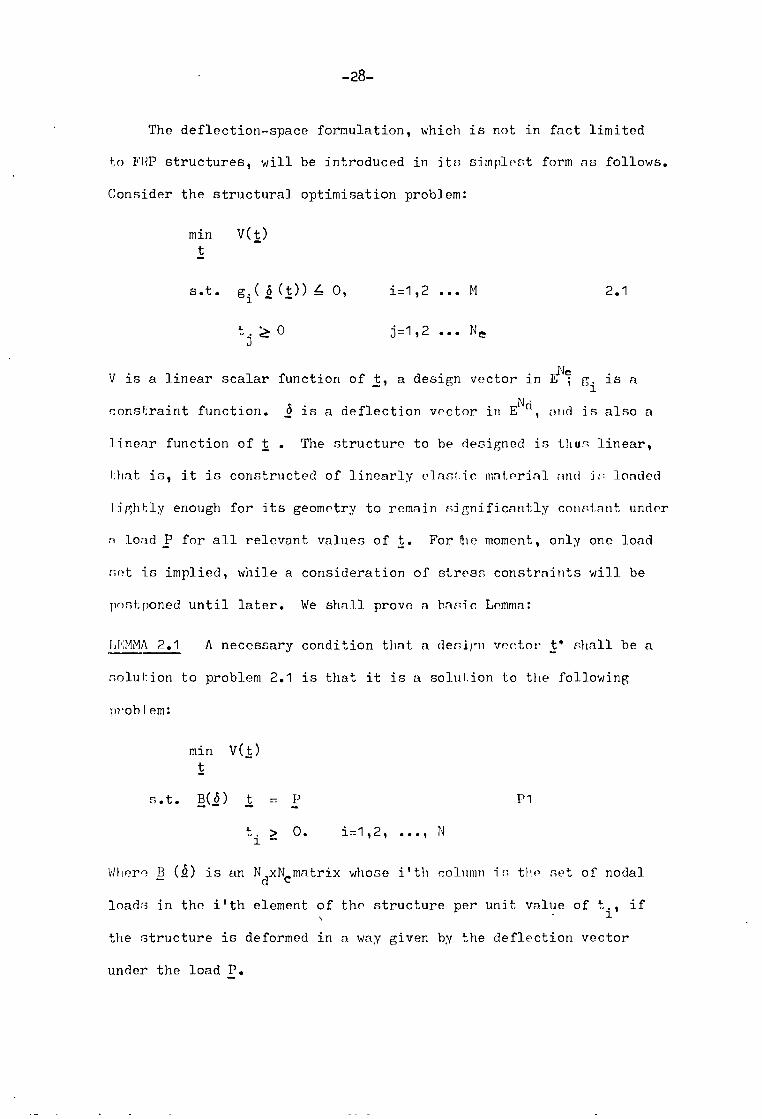
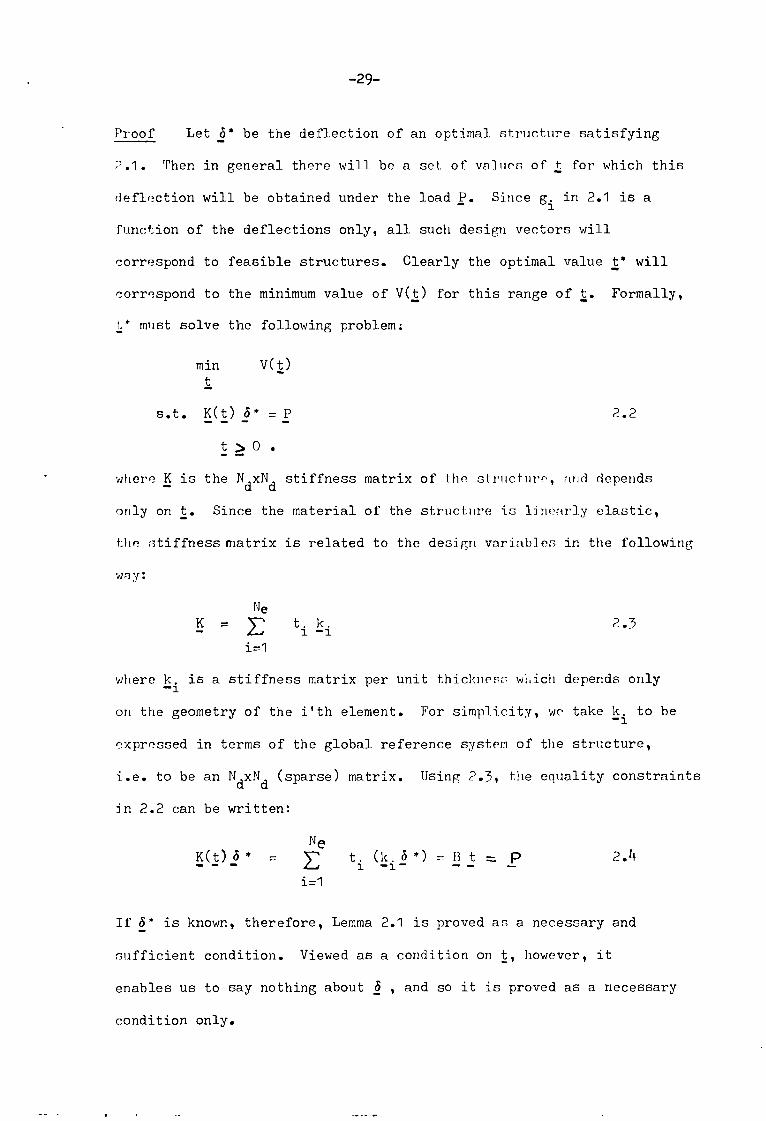
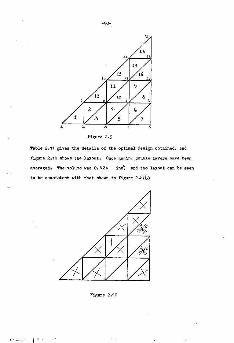
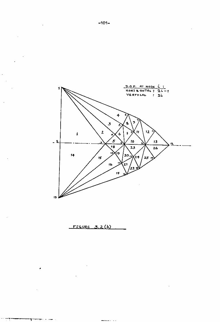
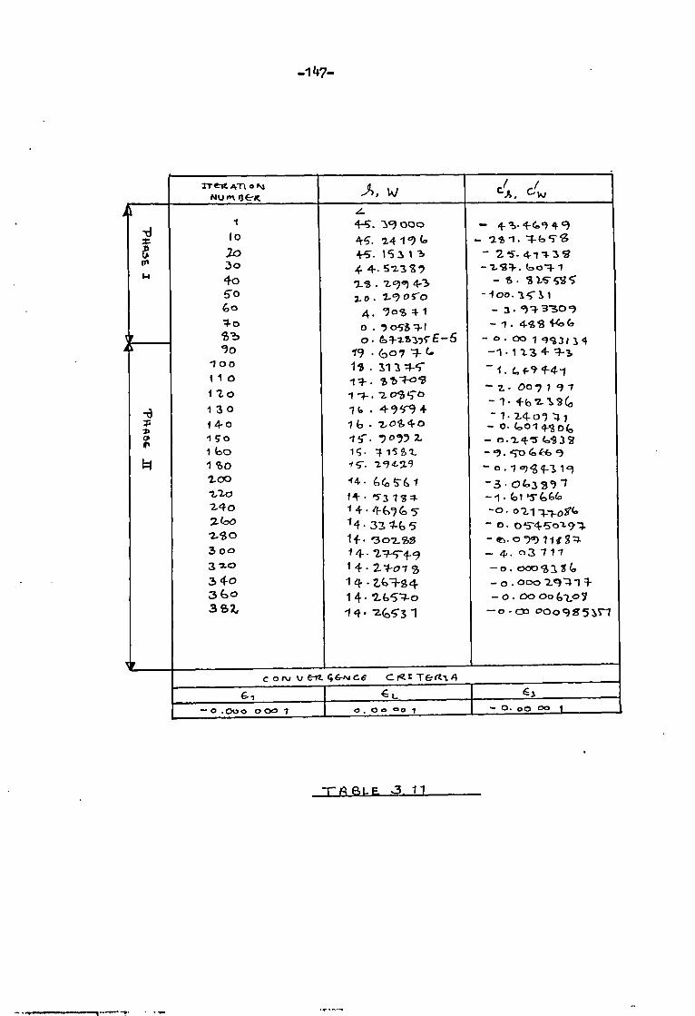
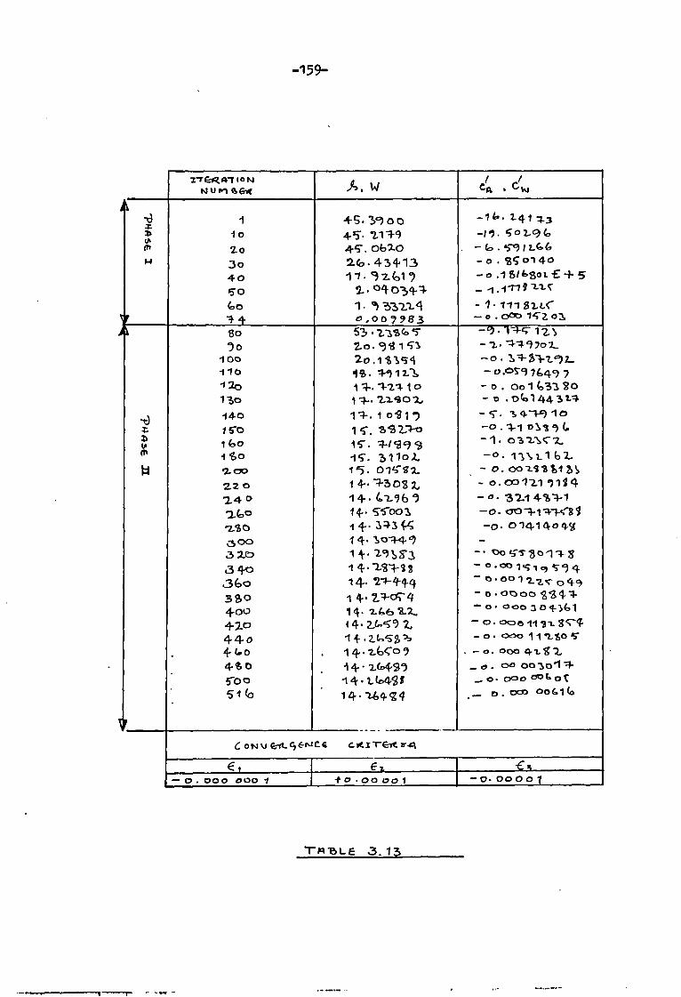
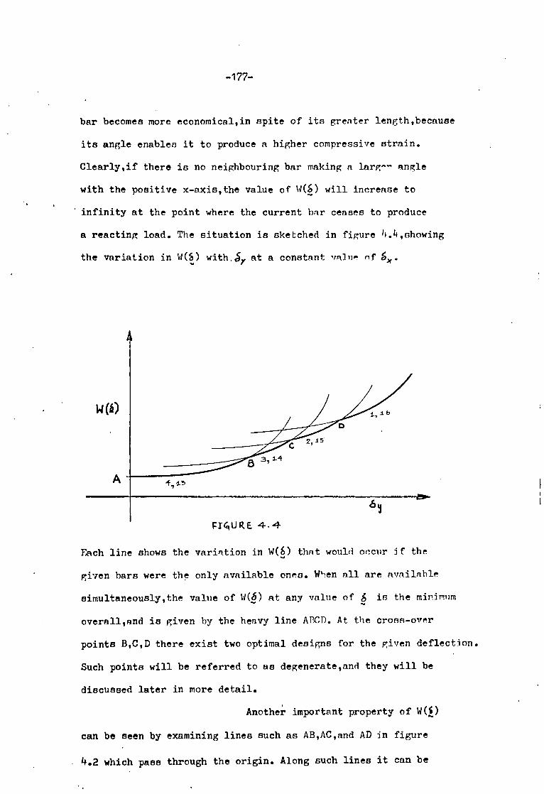
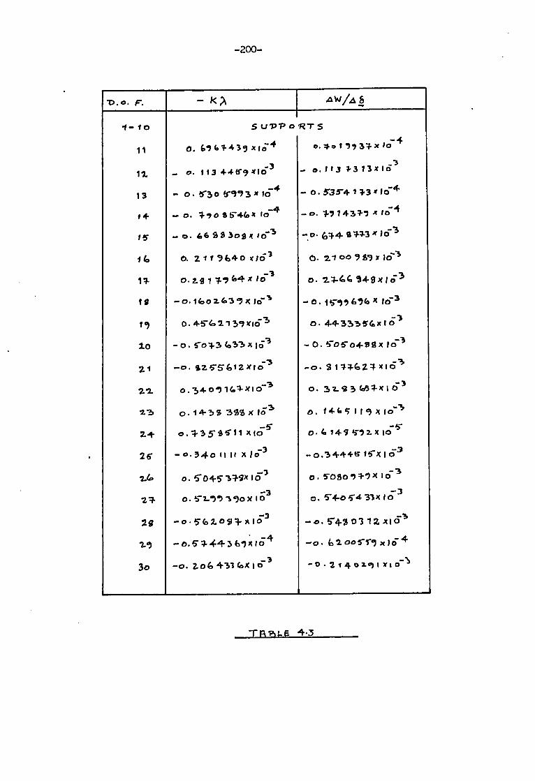
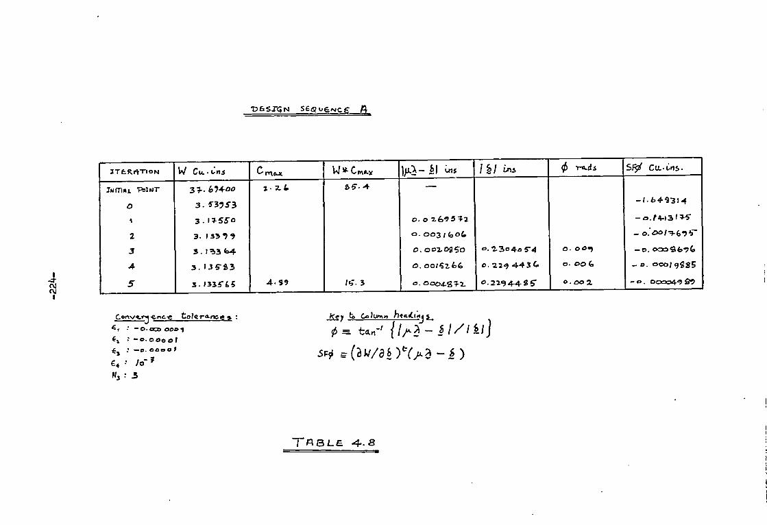
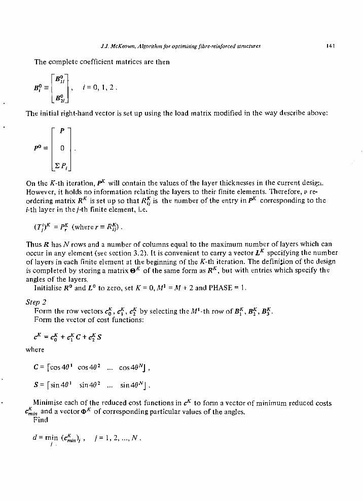
9 6 16 Pay- . Co-e6-tkm ,t4 . -ILA,/ k.., cilio.ovv1,4 2 • I , ..- -k 2...g,
iNA 644,1, 3 • 1 , 'w -t 2 . I
,9 ( I I Ai k (1)-1- / tA1 4- I.
10 C-K/ 0131 G , (ato-,t. c tis 61,trit
g-o : 619/0_91-0U1k 2 ' ,
I 4;2 F • 4.1 1- at4LA, 10rt
190 1-71 .4.. If part a-7 = (-wiz .