by Soumil Chugh

An Eye Tracking System for a Virtual Reality Headset

by

Soumil Chugh

A thesis submitted in conformity with the requirementsfor the degree of Masters of Applied Science

Graduate Department of Electrical and Computer EngineeringUniversity of Toronto

c© Copyright 2020 by Soumil Chugh

Abstract

An Eye Tracking System for a Virtual Reality Headset

Soumil Chugh

Masters of Applied Science

Graduate Department of Electrical and Computer Engineering

University of Toronto

2020

This research describes a head-mounted eye tracking system for a commercial virtual reality (VR) system.

The system uses infrared LEDs that illuminate the eyes and cameras to capture eye images and a 3D

gaze estimation model that uses the locations pupil center and corneal reflections in the eye images. It

generates gaze estimates that are insensitive to headset slippage. A key contribution of the work is a

novel method to determine the correspondence between the corneal reflections and the LEDs. This is

done using a fully convolutional neural network (CNN) based on the UNET architecture, which correctly

identifies and matches 91% of reflections in tests. The eye tracking system has an average gaze accuracy

of 1.1◦, which is at least 100% better than current VR eye tracking systems. The high accuracy of the

system was maintained with up to 10 mm of headset slippage.

ii

Acknowledgements

I want to thank my supervisors Prof. Jonathan Rose and Prof. Moshe Eizenman, for their invaluable

support and for giving me almost unlimited freedom during the past two years. I enjoyed the remarkable

learning experience you get when working with Prof. Rose and Prof. Eizenman. I also thank my co-

workers for providing support and assistance whenever I needed and making my time at UofT delightful.

I would also like to thank my family and friends for their continued support over the past two

years, driving me to do compelling research at UofT. Finally, I thank the Department of Electrical and

Computer Engineering, Huawei, and NSERC for funding this research.

iii

Contents

1 Introduction 1

1.1 Eye Tracking and its Applications . . . . . . . . . . . . . . . . . . . . . . . . . . . . . . . 1

1.2 Importance of Eye Tracking in XR systems . . . . . . . . . . . . . . . . . . . . . . . . . . 1

1.3 XR vs non-XR systems . . . . . . . . . . . . . . . . . . . . . . . . . . . . . . . . . . . . . 3

1.4 Challenges . . . . . . . . . . . . . . . . . . . . . . . . . . . . . . . . . . . . . . . . . . . . . 4

1.5 Contributions . . . . . . . . . . . . . . . . . . . . . . . . . . . . . . . . . . . . . . . . . . . 4

1.6 Thesis Organization . . . . . . . . . . . . . . . . . . . . . . . . . . . . . . . . . . . . . . . 4

2 Background and Prior Work 6

2.1 Virtual Reality System . . . . . . . . . . . . . . . . . . . . . . . . . . . . . . . . . . . . . . 6

2.1.1 Hardware . . . . . . . . . . . . . . . . . . . . . . . . . . . . . . . . . . . . . . . . . 6

2.1.2 Software . . . . . . . . . . . . . . . . . . . . . . . . . . . . . . . . . . . . . . . . . . 8

2.1.3 VR Coordinate Systems . . . . . . . . . . . . . . . . . . . . . . . . . . . . . . . . . 8

2.2 Eye Tracking . . . . . . . . . . . . . . . . . . . . . . . . . . . . . . . . . . . . . . . . . . . 9

2.2.1 Camera Configuration of Eye Trackers in XR systems . . . . . . . . . . . . . . . . 9

2.2.2 Pupil Labs Module for a VR Headset . . . . . . . . . . . . . . . . . . . . . . . . . 9

2.2.3 Eye Tracking Methods . . . . . . . . . . . . . . . . . . . . . . . . . . . . . . . . . . 11

2.2.4 Feature Extraction Methods . . . . . . . . . . . . . . . . . . . . . . . . . . . . . . . 16

3 End-to-End Eye Tracking Software System 20

3.1 Pupil Capture Application . . . . . . . . . . . . . . . . . . . . . . . . . . . . . . . . . . . . 21

3.2 3D scene for Calibration/Testing . . . . . . . . . . . . . . . . . . . . . . . . . . . . . . . . 21

3.3 Eye Tracking Algorithm . . . . . . . . . . . . . . . . . . . . . . . . . . . . . . . . . . . . . 21

3.3.1 Feature Extractor . . . . . . . . . . . . . . . . . . . . . . . . . . . . . . . . . . . . 21

3.3.2 Gaze Estimator . . . . . . . . . . . . . . . . . . . . . . . . . . . . . . . . . . . . . . 22

3.3.3 Calibrator . . . . . . . . . . . . . . . . . . . . . . . . . . . . . . . . . . . . . . . . . 24

3.4 Physical System Configuration . . . . . . . . . . . . . . . . . . . . . . . . . . . . . . . . . 25

3.5 Gaze Visualisation . . . . . . . . . . . . . . . . . . . . . . . . . . . . . . . . . . . . . . . . 25

4 Corneal Reflections Detection and Matching 27

4.1 Network Architecture . . . . . . . . . . . . . . . . . . . . . . . . . . . . . . . . . . . . . . 28

4.1.1 Objective Function . . . . . . . . . . . . . . . . . . . . . . . . . . . . . . . . . . . . 28

4.2 Data Collection . . . . . . . . . . . . . . . . . . . . . . . . . . . . . . . . . . . . . . . . . . 29

4.3 Data Labelling . . . . . . . . . . . . . . . . . . . . . . . . . . . . . . . . . . . . . . . . . . 30

iv

4.4 Dataset Generation . . . . . . . . . . . . . . . . . . . . . . . . . . . . . . . . . . . . . . . . 31

4.5 Data Augmentation . . . . . . . . . . . . . . . . . . . . . . . . . . . . . . . . . . . . . . . 32

4.6 Post Processing . . . . . . . . . . . . . . . . . . . . . . . . . . . . . . . . . . . . . . . . . . 32

4.7 Artificial Spurious Reflections vs Real Corneal Reflections . . . . . . . . . . . . . . . . . . 33

4.8 Dataset Splitting . . . . . . . . . . . . . . . . . . . . . . . . . . . . . . . . . . . . . . . . . 34

4.9 Hyperparameter Tuning . . . . . . . . . . . . . . . . . . . . . . . . . . . . . . . . . . . . . 35

4.9.1 Specific Hyperparameters Explored . . . . . . . . . . . . . . . . . . . . . . . . . . . 35

4.10 Training/Exploration Process . . . . . . . . . . . . . . . . . . . . . . . . . . . . . . . . . . 36

4.11 Corneal Reflection Detection and Matching Performance on the Test Dataset . . . . . . . 37

4.12 Feature Extractor Performance Comparison with State-of-the-art Methods . . . . . . . . . 38

4.13 Corneal Reflection Pair Accuracy . . . . . . . . . . . . . . . . . . . . . . . . . . . . . . . . 39

4.14 Effect of Spurious Reflections . . . . . . . . . . . . . . . . . . . . . . . . . . . . . . . . . . 40

4.15 Real Time Performance of the Network . . . . . . . . . . . . . . . . . . . . . . . . . . . . 40

4.16 Selection of Corneal Reflections for Gaze Estimation . . . . . . . . . . . . . . . . . . . . . 41

5 Pupil Center Estimation 43

5.1 Data Collection . . . . . . . . . . . . . . . . . . . . . . . . . . . . . . . . . . . . . . . . . . 43

5.2 Data Labelling . . . . . . . . . . . . . . . . . . . . . . . . . . . . . . . . . . . . . . . . . . 43

5.3 Objective Function . . . . . . . . . . . . . . . . . . . . . . . . . . . . . . . . . . . . . . . . 44

5.4 Post Processing . . . . . . . . . . . . . . . . . . . . . . . . . . . . . . . . . . . . . . . . . . 45

5.5 Hyperparameter Tuning Results . . . . . . . . . . . . . . . . . . . . . . . . . . . . . . . . 46

5.6 Pupil Center Estimation Performance on Test Dataset . . . . . . . . . . . . . . . . . . . . 48

5.7 Performance Comparison with State-of-the-art Methods . . . . . . . . . . . . . . . . . . . 49

5.8 Real Time Performance of the Network . . . . . . . . . . . . . . . . . . . . . . . . . . . . 50

5.9 Effect of Boundary Aware Loss Function . . . . . . . . . . . . . . . . . . . . . . . . . . . . 50

5.10 Gaze Estimation Rate . . . . . . . . . . . . . . . . . . . . . . . . . . . . . . . . . . . . . . 51

6 Eye Tracking Results 52

6.1 Eye Tracking Performance with no Headset slippage . . . . . . . . . . . . . . . . . . . . . 52

6.1.1 Performance Metrics . . . . . . . . . . . . . . . . . . . . . . . . . . . . . . . . . . . 53

6.1.2 Eye tracking Performance . . . . . . . . . . . . . . . . . . . . . . . . . . . . . . . . 53

6.2 Comparison with State-of-the-art Eye Tracking Systems . . . . . . . . . . . . . . . . . . . 54

6.3 Testing the System at a Larger Field of View . . . . . . . . . . . . . . . . . . . . . . . . . 56

6.4 Eye Tracking Performance with Headset Slippage . . . . . . . . . . . . . . . . . . . . . . . 56

7 Conclusion and Future Work 63

7.1 Conclusion . . . . . . . . . . . . . . . . . . . . . . . . . . . . . . . . . . . . . . . . . . . . 63

7.2 Future Work . . . . . . . . . . . . . . . . . . . . . . . . . . . . . . . . . . . . . . . . . . . 64

7.2.1 Use of On-Axis Camera Configuration . . . . . . . . . . . . . . . . . . . . . . . . . 64

7.2.2 Synchronization Between Camera and Light sources . . . . . . . . . . . . . . . . . 64

7.2.3 Reducing the Effects of Lens Distortion . . . . . . . . . . . . . . . . . . . . . . . . 65

7.2.4 Eye tracking System for Augmented or Mixed Reality . . . . . . . . . . . . . . . . 65

v

A Hyperparameter Tuning Results 66

A.1 Hyperparameter Results for the Pupil Center Estimation Network . . . . . . . . . . . . . 66

A.2 Hyperparameter Results for the Corneal Reflection Detection and Matching Network . . . 67

Bibliography 67

vi

List of Tables

3.1 Calibration Parameters . . . . . . . . . . . . . . . . . . . . . . . . . . . . . . . . . . . . . 25

3.2 Physical System Parameters . . . . . . . . . . . . . . . . . . . . . . . . . . . . . . . . . . . 25

4.1 Hyperparameters Explored . . . . . . . . . . . . . . . . . . . . . . . . . . . . . . . . . . . 36

4.2 Unchanged Hyperparameters . . . . . . . . . . . . . . . . . . . . . . . . . . . . . . . . . . 36

4.3 Results for Corneal reflection Detection and Matching when max pooling used as down-

sampling with Biliner Interpolation as upsampling layer . . . . . . . . . . . . . . . . . . . 37

4.4 Performance metrics based on number of valid reflections present in the image . . . . . . 38

4.5 Accuracy of pair detection as a function of number of valid corneal reflections . . . . . . . 39

5.1 Hyperparameter tuning results for the networks which uses Strided Convolution in each

of the four downsampling blocks and Transposed CNN in each of the four upsampling

blocks . . . . . . . . . . . . . . . . . . . . . . . . . . . . . . . . . . . . . . . . . . . . . . . 47

5.2 Pupil Center Estimation Network Performance on the Test dataset . . . . . . . . . . . . . 49

5.3 Comparison with Rule based algorithms on the test dataset . . . . . . . . . . . . . . . . . 49

5.4 Pupil Detection Rate (%) on LPW and Swriski Datasets . . . . . . . . . . . . . . . . . . . 50

6.1 Comparison with non-XR systems . . . . . . . . . . . . . . . . . . . . . . . . . . . . . . . 54

6.2 Comparison with learning based XR systems (◦) . . . . . . . . . . . . . . . . . . . . . . . 55

6.3 Mean Accuracy during headset slippage (◦) . . . . . . . . . . . . . . . . . . . . . . . . . . 58

A.1 Hyperparameter results for pupil center networks when used Strided Convolution in the

four downsampling blocks and Bilinear Interpolation in the four upsampling blocks . . . . 66

A.2 Hyperparameter results for pupil center networks when used Strided Convolution in each

of three downsampling blocks and Bilinear Interpolation in each of the three upsampling

blocks . . . . . . . . . . . . . . . . . . . . . . . . . . . . . . . . . . . . . . . . . . . . . . . 66

A.3 Hyperparameter results for pupil center networks when used Max Pooling in each of the

four downsampling blocks and Transposed CNN in each of the four upsampling blocks. . . 67

A.4 Hyperparameter results for pupil center networks when using Max Pooling in each of the

three downsampling blocks and Transposed CNN in each of the three upsampling blocks . 67

A.5 Hyperparameter results for corneal reflections networks when max pooling used as down-

sampling with Bilinear Interpolation as upsampling layer. Number of blocks set to 3 . . . 68

A.6 Hyperparameter results for corneal reflections networks when max pooling used as down-

sampling with Transposed CNN as upsampling layer. Number of blocks set to 4 . . . . . . 68

vii

A.7 Hyperparameter results for corneal reflections networks when strided CNN used as down-


A.8 Hyperparameter results for corneal reflections networks when strided CNN used as down-


viii

List of Figures

1.1 Commercially available XR systems . . . . . . . . . . . . . . . . . . . . . . . . . . . . . . 2

1.2 VR Eye Tracking System . . . . . . . . . . . . . . . . . . . . . . . . . . . . . . . . . . . . 3

1.3 Commercially available non-XR systems . . . . . . . . . . . . . . . . . . . . . . . . . . . . 3

2.1 HTC Vive Virtual Reality Headset . . . . . . . . . . . . . . . . . . . . . . . . . . . . . . . 6

2.2 Lenses and Displays inside HTC Vive . . . . . . . . . . . . . . . . . . . . . . . . . . . . . 7

2.3 Comparison between two camera configurations as shown in [1]. Figure a) represents the

off-axis camera configuration. Figure b) shows the on-axis camera configuration . . . . . 9

2.4 Pupil Labs Module inside the HTC Vive headset . . . . . . . . . . . . . . . . . . . . . . . 10

2.5 Eye images captured from Pupil Labs Module . . . . . . . . . . . . . . . . . . . . . . . . . 10

2.6 Standard Convolution (left) vs Dilated Convolution (right) . . . . . . . . . . . . . . . . . 13

2.7 Depth-Wise Convolution followed by 1x1 Standard Convolution . . . . . . . . . . . . . . . 14

2.8 Upsampling using Transposed CNN . . . . . . . . . . . . . . . . . . . . . . . . . . . . . . 14

2.9 Eye images recorded with different eye tracking systems under varying environments . . . 17

2.10 The five Corneal reflections generated by five IR light sources inside a VR headset . . . . 18

3.1 Software Architecture . . . . . . . . . . . . . . . . . . . . . . . . . . . . . . . . . . . . . . 20

3.2 Eye Tracking Software System . . . . . . . . . . . . . . . . . . . . . . . . . . . . . . . . . 22

3.3 Components of the VR eye tracking system . . . . . . . . . . . . . . . . . . . . . . . . . . 22

3.4 The calibration points at ±5◦are denoted by color red. Blue (±10◦) and green color points

(±15◦) are the test points that will be used to evaluate the system. . . . . . . . . . . . . . 24

4.1 UNET Style Architecture . . . . . . . . . . . . . . . . . . . . . . . . . . . . . . . . . . . . 28

4.2 Images labelled with true corneal reflections for each of the light sources. Red denotes

Light Source 1, Orange denotes Light Source 2, Pink denotes Light Source 3, Green

denotes Light Source 4, and Blue denotes Light source 5. . . . . . . . . . . . . . . . . . . 30

4.3 Binary Masks for each of the corneal reflections for the Labelled image in 4.2 . . . . . . . 31

4.4 Images after data augmentation . . . . . . . . . . . . . . . . . . . . . . . . . . . . . . . . . 33

4.5 Post-processing results for one of the corneal reflections . . . . . . . . . . . . . . . . . . . 33

4.6 Validation and Test Datasets Distribution based on the number of valid corneal reflections

present in the image . . . . . . . . . . . . . . . . . . . . . . . . . . . . . . . . . . . . . . . 34

4.7 ROC for each of the Corneal Reflections . . . . . . . . . . . . . . . . . . . . . . . . . . . . 38

4.8 Bounding box indicates the region where the artificial reflections were added. The black

labelled regions are the corneal reflections, while all other bright dots are spurious reflections. 40

4.9 Pair Accuracy closest to Pupil Center vs Spurious Reflections . . . . . . . . . . . . . . . . 40

ix

4.10 Pair Accuracy vs Spurious Reflections . . . . . . . . . . . . . . . . . . . . . . . . . . . . . 41

4.11 Selection of different corneal reflections based on the gaze position. The reflections marked

with red, orange, pink, green and blue represent the different corneal reflections in the

image. Only the reflections falling inside the boundary region (denoted by white) are

considered for gaze estimation. . . . . . . . . . . . . . . . . . . . . . . . . . . . . . . . . . 42

5.1 Effect of changing illumination in the 3D scene on the pupil size . . . . . . . . . . . . . . 44

5.2 Example cases of the valid and invalid eye images . . . . . . . . . . . . . . . . . . . . . . . 45

5.3 Labelled eye images with pupil boundary denoted with colour Red . . . . . . . . . . . . . 45

5.4 Post processing . . . . . . . . . . . . . . . . . . . . . . . . . . . . . . . . . . . . . . . . . . 46

5.5 ROC for Pupil Network . . . . . . . . . . . . . . . . . . . . . . . . . . . . . . . . . . . . . 48

5.6 Eye images from the two publicly available datasets . . . . . . . . . . . . . . . . . . . . . 50

5.7 Occluded valid eye images labelled with pupil boundary . . . . . . . . . . . . . . . . . . . 51

6.1 Raw gaze estimates at ± 10◦for the nine target position at 1m fixation distance . . . . . . 54

6.2 Performance metrics for target points placed at ±10 ◦ . . . . . . . . . . . . . . . . . . . . 55

6.3 Raw gaze estimates at ± 15◦for every target position . . . . . . . . . . . . . . . . . . . . . 56

6.4 Performance metrics at ± 15◦ . . . . . . . . . . . . . . . . . . . . . . . . . . . . . . . . . . 57

6.5 Gaze estimates, target locations and headset position during no headset slippage . . . . . 59

6.6 Gaze estimates, target locations and headset position during the up/down movement of

the headset . . . . . . . . . . . . . . . . . . . . . . . . . . . . . . . . . . . . . . . . . . . . 60

6.7 Gaze estimates, target locations and headset position during the left/right movement of

the headset . . . . . . . . . . . . . . . . . . . . . . . . . . . . . . . . . . . . . . . . . . . . 62

7.1 Tobii VR . . . . . . . . . . . . . . . . . . . . . . . . . . . . . . . . . . . . . . . . . . . . . 65

x

Chapter 1

Introduction

1.1 Eye Tracking and its Applications

People move their eyes to gather information. An eye tracking or gaze estimation device tracks eye

movements and continuously estimates where a subject is looking. This capability of eye tracking

systems support applications in domains that include mental health [2, 3, 4], gaming [5, 6, 7], marketing

[8], automotive safety [9], and human-computer interaction[10, 11, 12].

Video-based eye tracking is the most widely used input basis for gaze estimation. These systems

consists of a camera for capturing eye images and light sources to illuminate the eyes. Video-based

eye tracking systems are further categorized into 1) Remote systems, typically desktop system where

the camera is placed far away from the eye, and 2) Head-mounted systems where the camera and light

sources are closer to the eye. We focus our research on head-mounted systems that are designed for

extended reality systems.

Extended Reality (XR) includes a set of computer-generated experiences that extend the real world

through virtual simulation or augmentation. The technologies that enable such experiences include

virtual reality (VR), augmented reality (AR) and mixed reality (MR). In AR, the physical world overlays

virtual content, while VR creates a fully computer-generated 3D virtual world. MR, on the other hand,

merges AR and VR.

XR systems have hardware capabilities to generate 3D graphics, spatialized sound and motion track-

ing necessary for simulated and augmented user experiences. The form factor of all XR systems is a

head-mounted system with integrated display screens and lenses for each eye. Commercially available

head-mounted AR, MR and VR systems can be seen in Figure 1.1.

The popularity of XR systems has led to increased interest in the use of eye tracking within the XR

system. We elaborate on the use of eye tracking in XR systems in the next section.

1.2 Importance of Eye Tracking in XR systems

The rise in the adoption of XR systems in recent years can largely be attributed to the field of gaming

[13]. However, XR technology has also shown potential to enhance human experiences in areas such as

education and training[14], healthcare[15], marketing[16], and sports [17].

There are many benefits of integrating eye tracking into XR systems. One of the significant hurdles

1

Chapter 1. Introduction 2

(a) AR system(b) VR system

(c) MR system

Figure 1.1: Commercially available XR systems

to XR adoption has been the high cost, partly caused by the high graphics processing requirements of

current XR systems. The XR system’s displays must maintain high-resolution at all times for an im-

mersive user experience, which increases computational cost. Foveated rendering [18] saves considerable

computing resources by using the gaze information from the eye tracker, allowing the peripheral image

to degrade in a way that is unobtrusive for the user while rendering only the area of the display where

the user is looking.

Eye tracking also enables the use of multifocal displays to reduce the vergence accommodation effect

[19]. This occurs when the brain receives mismatching cues between the object’s actual distance from

the eye (vergence), and the focusing distance (accommodation) required for the eyes to focus on that

object. In XR systems, the focusing distance is fixed, while objects in the 3D world can move in the

virtual space. This conflict contributes to visual fatigue, especially during prolonged use of XR devices

[20, 21]. It can also, for some people, cause serious side-effects. Variable-focus lenses could allow the

lens’s focusing distance to change with the change in eye-gaze distance in the virtual 3D scene.

Eye tracking can also improve user interaction in XR devices, which is usually done using haptic,

hand, head and motion tracking, and can be slow and tedious [22]. Gaze-based interaction has been

shown to be faster and more natural [23, 24].

For these reasons, eye tracking may play a pivotal role in the future of XR devices. There are four

fundamental requirements that an eye tracking system has to satisfy for this to be possible:

• Gaze estimation should be highly accurate.

• Gaze estimation accuracy should be maintained regardless of the fixation distance in the 3D scene.

• Gaze estimation accuracy should not be affected by the eye tracker’s movement relative to the

head. These movements, also known as headset slippage, result from head movements, or user

adjustment of the headset (which can cause displacements as large as 10mm).


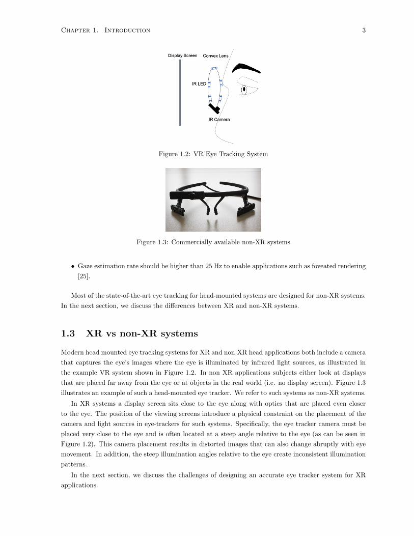
Figure 1.2: VR Eye Tracking System

Figure 1.3: Commercially available non-XR systems

• Gaze estimation rate should be higher than 25 Hz to enable applications such as foveated rendering

[25].

Most of the state-of-the-art eye tracking for head-mounted systems are designed for non-XR systems.

In the next section, we discuss the differences between XR and non-XR systems.

1.3 XR vs non-XR systems

Modern head mounted eye tracking systems for XR and non-XR head applications both include a camera

that captures the eye’s images where the eye is illuminated by infrared light sources, as illustrated in

the example VR system shown in Figure 1.2. In non XR applications subjects either look at displays

that are placed far away from the eye or at objects in the real world (i.e. no display screen). Figure 1.3

illustrates an example of such a head-mounted eye tracker. We refer to such systems as non-XR systems.

In XR systems a display screen sits close to the eye along with optics that are placed even closer

to the eye. The position of the viewing screens introduce a physical constraint on the placement of the

camera and light sources in eye-trackers for such systems. Specifically, the eye tracker camera must be

placed very close to the eye and is often located at a steep angle relative to the eye (as can be seen in

Figure 1.2). This camera placement results in distorted images that can also change abruptly with eye

movement. In addition, the steep illumination angles relative to the eye create inconsistent illumination

patterns.

In the next section, we discuss the challenges of designing an accurate eye tracker system for XR

applications.


1.4 Challenges

Our eye tracking system makes use of the 3D gaze estimation model [26], which requires precise estimation

of two eye features: locations of the pupil center and the locations of the virtual images of the IR light

sources created by reflections from the cornea [26]. We will refer to these latter virtual images as

corneal reflections. Example corneal reflections can be seen in Figure 2.10. Information regarding the

correspondence between the reflection and its originating LED also needs to be known to our system

[26].

The combination of poor quality eye images, and physical constraints make accurate eye feature

extraction for XR systems prone to errors. Also, failures to match corneal reflections with its corre-

sponding light sources increases due to: corneal reflections having varying shape and intensity levels,

corneal reflections disappearing due to rotation of the eye, or the presence of spurious reflections.

In a previous paper, authors demonstrated that deep learning-based eye feature extraction methods

could be more accurate and robust [27] than traditional handcrafted computer vision methods [28]. This

leads to the contributions of this work, which is discussed next.

1.5 Contributions

The main contributions of this thesis are:

• Developing a novel corneal reflection detection and matching algorithm using a fully convolutional

neural network. The proposed approach is based on the UNET architecture [29] which correctly

identify and matches 91% of corneal reflections in the test dataset.

• Developing an accurate end-to-end eye tracking system using the 3D gaze estimation model that

runs on an HTC Vive VR headset [30] with a binocular eye tracking module manufactured by

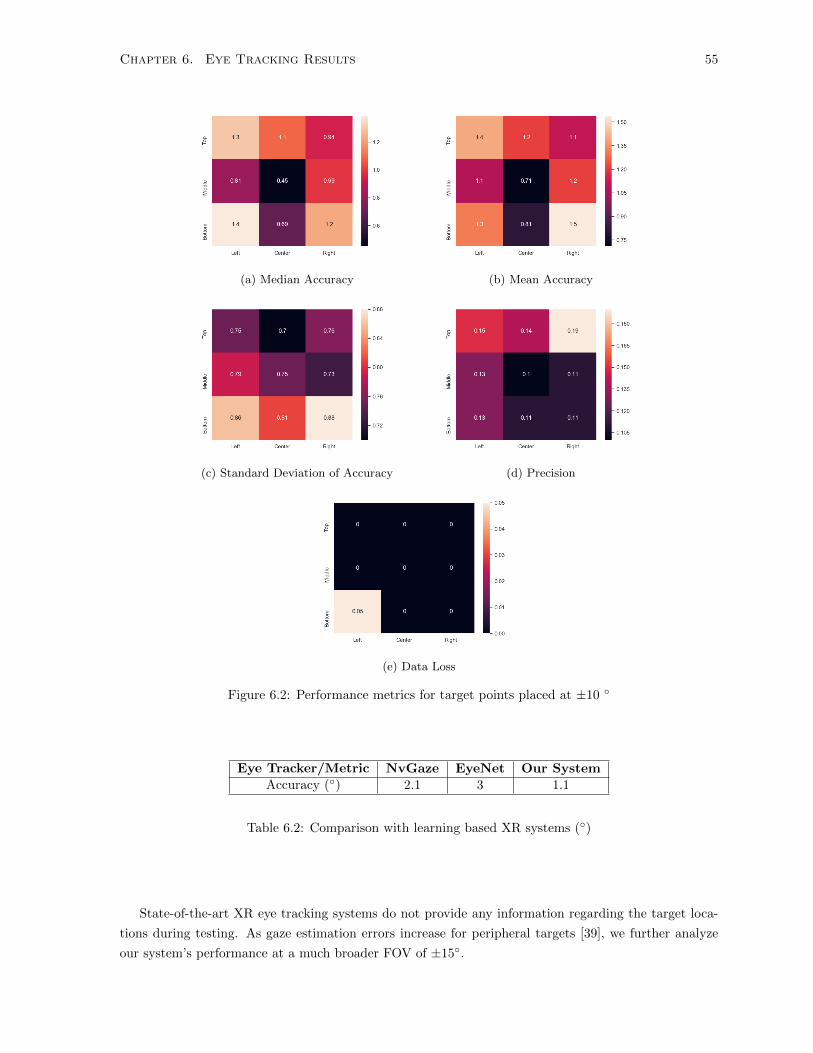
Pupil Labs [31]. Our system reports an accuracy (median) of 1◦ in the central field of view (FOV)

of ±10◦ and 1.6◦ in FOV of ±15◦. These results are reported after testing the system on six

different subjects at different fixation distances. We compare the system’s performance with the

state-of-the-art XR [1, 32] and non-XR systems [33]. Our system accuracy for the field of view

of ±10◦ is 40% higher than state-of-the-art non-XR systems and at least 100% better than XR

eye tracking systems. With headset slippage of up to 10mm when the subject focuses on the most

central point in the display, the average accuracy decreases from 0.6◦ to 1.9◦. This is comparable

to the state-of-the-art non-XR systems.

In the next section, we provide an outline for the thesis.

1.6 Thesis Organization

The organization of the remainder of the thesis is as follows: Chapter 2 provides background information

on Virtual Reality and eye tracking systems. This involves a discussion regarding the software and

hardware components of a VR system. Chapter 2 also covers topics including state-of-the-art gaze

estimation techniques and the front-end feature extraction methods that employ them. Chapter 3 gives

a top-level overview of the software architecture for the end-end eye tracking system. Chapters 4 and

5 describe the feature extractions networks that include corneal reflection detection and matching, and


pupil center estimation. Chapter 6 presents the end-to-end eye tracking system results with a detailed

comparison with the existing XR and non-XR head-mounted eye trackers. Finally, Chapter 7 offers

conclusions and directions for future work.

Chapter 2

Background and Prior Work

This chapter describes the components of the Virtual Reality (VR) system that we build on and provides

a review of eye tracking algorithms and systems. The discussion of the VR system includes both software

and hardware aspects of such systems. The discussion of eye tracking systems includes an overview of

head-mounted eye tracking systems and methods to estimate eye-features used to determine the point-

of-gaze in such systems.

2.1 Virtual Reality System

A VR system uses computer technology to create a simulated 3D environment that can be explored by

a person. In this section, we described the hardware components involved.

2.1.1 Hardware

The hardware components are responsible for generating and interacting with the 3D virtual world. The

components consist of a processor, headset, sensors and controllers. The processor generates images of

a virtual world displayed on a screen within the headset while sensors and controllers enable real-time

interactions with 3D objects in the virtual world. VR systems measure motion of the head in the headset

using an inertial measurement unit (IMU) that includes gyroscopes and accelerometers. There is also a

set of hand-held controllers that can be driven by touch, that enable real-time interaction with the VR

environment.

Figure 2.1: HTC Vive Virtual Reality Headset

Our prototype eye tracking system uses an HTC Vive [34] VR system which is illustrated in Figure

2.1.

6

Chapter 2. Background and Prior Work 7

Below we discuss the hardware components of the HTC Vive VR headset used in this work.

Display

HTC Vive consists of two displays (OLED or LCD) one for each of the eyes. These displays have a

resolution of 1080x1200 per eye running at 90Hz. Convex lenses are placed between the displays and

the eyes to magnify and project display to a comfortable viewing distance. This viewing distance is said

to be approximately 75cm (equivalent to 1 arms-length). The projected magnified image of the display

is the 3D virtual scene that the user sees. An inside view of the HTC Vive VR headset can be seen in

Figure 2.2.

Figure 2.2: Lenses and Displays inside HTC Vive

Sensors

HTC Vive enables rotational and positional tracking required for the control of the virtual world content

when users move and rotate their heads in the real world. While rotational tracking is achieved using

a gyroscope, positional tracking is done using an accelerometer. The accelerometer sensor provides the

headset’s position in 3D world coordinates by double integration of the measured acceleration. Double

integration is very sensitive to drifts in the measured acceleration, and within a matter of seconds, the

positional tracking can be off by a significant factor. To overcome this problem, the HTC Vive headset

has an array of infrared photo-diodes sensors on its outer covering and base-stations (”Lighthouses”)

that emit two dimensional IR laser beams that sweep across the room one axis at a time, repeatedly.

These lighthouses are squared shaped sensors, as can be seen in Figure 2.1. Before each sweep, the

base-stations emit a powerful IR flash of light. A chip embedded inside the VR headset measures the

time between the IR flash and the response of the photo-diodes sensors to each axis’s sweeping laser

beam. From this information, along with the accelerometer data, the headset position in the room is

determined. Tracking headset positions in real-time are often termed head tracking (assuming that the

headset does not slip on the user’s head). In the HTC, the head tracking information is transferred to

the processor (i.e., the Virtual World Generator running on a PC) using wired communication. Based

on this information, the Virtual World Generator updates the 3D scene.

Processor

The processor is responsible for running the virtual world generator (VWG) and sending out the in-

formation to be displayed on the VR headset’s display. In addition to the central processor, most VR


headsets require specialized additional computing hardware for rendering displays at high resolutions

with a high frame rate. This task is usually accomplished by Graphical processing units (GPUs) that

are optimized for fast rendering of graphics to a screen. In the next section, we discuss the main software

modules of VR systems.

2.1.2 Software

A VR software engine running on a PC is responsible for generating the virtual world/ 3D scene. The

VR software engine updates the 3D scene using the information from the head tracker and other sensors

in the system.

The most popular VWG engines are OpenSimulator [35], Unity 3D [36], and Unreal Engine[37] by

Epic Games. These engines allow the user to customize a particular VR experience by choosing menu

options and writing high-level scripts.

We selected Unity 3D[36] due to its popularity and extensive developer support. In the next section,

we provide a detailed description of the Unity3D software.

Unity3D Software Engine

Unity 3D is a cross-platform game engine used for designing 2D games and XR applications [36]. Unity

allows the creation of 3D objects such as spheres, cubes, and cylinders, also called ‘GameObjects’ in

the 3D scene. Every GameObject has components attached, which control its behaviour. For instance,

a transform component controls the position, orientation and size of the GameObject. Unity allows

creating new components using scripts. These scripts are programmed in a particular language that

Unity can understand called C#. Using scripts, Unity allows changing the GameObject properties over

time, trigger events and respond to events. GameObjects in a 3D scene are placed relative to a coordinate

system. The different coordinate systems in a 3D scene are discussed next.

2.1.3 VR Coordinate Systems

There are two coordinate systems in a 3D scene: the virtual world coordinate system and the virtual

camera coordinate system. These coordinates systems are discussed next.

A 3D scene is defined relative to the virtual world coordinate system. This coordinate system is a

right-hand coordinate system and has three axes about which an object in a 3D scene is placed: x,y and

z. The coordinates in the virtual world are expressed in units of metres.

For a coordinate system, an origin must also be defined. In the virtual world coordinate system, this

is achieved by calibrating the VR system in the real world. The position of the VR device at the time

of calibration become the virtual world coordinate system’s origin. The orientations of the three axes of

the virtual world coordinate system are also determined during calibration. 3D objects fixed in the 3D

scene (i.e., objects that do not move with the user’s movements) are considered to be locked relative to

the world coordinate system.

A virtual world spreads across a field of view (FOV) of 110◦ around the user’s eye. However, a user

can only see and interact with the 3D objects that fall under the FOV of a virtual camera placed in the

3D scene. A virtual camera has its coordinate system known as a virtual camera coordinate system.

In this coordinate system, a 3D object is locked relative to the virtual camera. Placing an object in


the virtual camera coordinate system is usually done for a seated or standing the only experience. The

headset tracker controls the position and orientation of the virtual camera in the virtual world.

A transformation between the virtual world coordinate system and virtual camera coordinate system

can be done using the head tracker’s rotation and translation matrices. In the next section, we provide

an overview of the head-mounted eye tracking systems.

2.2 Eye Tracking

Video-based eye tracking systems for XR systems usually involve a camera to capture eye images and

light-emitting diodes for eye illumination. Infrared is the preferred source of eye illumination since it

does not interfere with the normal vision and provide good contrast between the pupil and iris for people

with brown irises.

The placement of the camera inside an XR system affects the quality of the captured eye images.

The possible camera placement configuration is discussed next.

2.2.1 Camera Configuration of Eye Trackers in XR systems

Cameras in XR systems can be placed on-axis or off-axis relative to the optical axis of the eye. These

two camera configurations can be seen in Figure 2.3.

The off-axis camera configuration occupies less space inside an XR headset, at the cost of accuracy

in gaze estimation [1]. On the other hand, the on-axis configuration requires more space but provides

a frontal view of the eye, which is better for accurate gaze estimation. Installing a camera in an on-

axis configuration requires modification in the physical design of an XR system. This modification is

beyond the scope of this research. The only other option is to consider off-axis camera configuration

since it requires an easy installation of cameras inside an XR system. For our system, we make use of a

commercially available off-axis eye tracking module, described next.

Figure 2.3: Comparison between two camera configurations as shown in [1]. Figure a) represents theoff-axis camera configuration. Figure b) shows the on-axis camera configuration

2.2.2 Pupil Labs Module for a VR Headset

Pupil Labs, an open-source eye tracking company, manufactures an off-axis eye tracking module for

AR/VR systems [31]. The hardware consists of a ring of five IR LEDs and an IR camera for each eye,

as illustrated in Figure 2.4. The IR light sources are placed evenly on the ring structure, with the IR


camera placed at the ring’s bottom. The camera images are streamed in real-time via a high-speed USB

3.0 connection to an application software called ’Pupil Capture’ running on a PC.

A CMOS camera sensor with a rolling shutter is present in the two eye cameras. The focus of these

cameras can be adjusted manually. The physical camera sensor for one of the cameras is flipped 180

degrees, which results in an inverted image. The camera’s image resolution can be set to four different

resolutions which include 320x240, 640x480, 1280x720 and 1920x1080. It is only at the resolution of

640x480, where frame rates within a range of 30-120 can be used. The captured left and right eye images

from this hardware can be seen in Figure 2.5.

Figure 2.4: Pupil Labs Module inside the HTC Vive headset

Pupil Capture application running on the PC, which controls the two eye cameras, associates a

timestamp with the captured images. This timestamp is the time at which the Pupil Capture software

receives the eye images from the cameras. Timestamps can be later used to synchronize the images from

the two eye cameras.

After selecting the hardware that can be used for gaze estimation, the next step is to select a gaze

estimation method. The next section describes the state-of-the-art gaze estimation methods, including

learning-based and geometrical methods used in XR and non-XR head-mounted systems. We then

discuss the recent eye feature extraction methods that employ rules-based approaches and deep learning-

based approaches, for pupil center and corneal reflection detection and correspondence matching.

(a) Left Eye Image (b) Right Eye Image

Figure 2.5: Eye images captured from Pupil Labs Module


2.2.3 Eye Tracking Methods

Head-mounted eye tracking systems employ gaze estimation methods that are broadly categorized into

a) feature-based (which directly use the location of features of the eye to compute gaze), b) model-based

(which explicitly model the anatomy of the eye and the eye tracking system) and c) appearance-based

(which directly compute gaze from an input eye image, such as a deep learning approach).

Feature Based Gaze estimation

Feature-based methods use spatial features of the eye to estimate the point of gaze. One of the popular

feature-based methods uses only the pupil center [38]. In this approach, using the results of a calibration

procedure, one computes a mapping function between the detected 2D pupil center in the eye image and

the 2D/3D gaze. The work in [39] uses this approach inside a VR headset with gaze estimates computed

in the screen coordinate system (X-Y plane). The authors report that the accuracy in gaze estimates for

all the 3D target points projected onto the 2D screen space is less than 1.5◦. In another approach [40],

a geometric transformation on the pupil center is applied to compute the gaze location on a 2D plane

inside an AR system. Testing only on calibration points (such a test suffers from less error) resulted in

a mean gaze estimation accuracy of 0.8◦.

The approaches discussed thus far compute gaze location in a 2D plane. To fully utilize the 3D

content of XR devices, eye trackers must generate point-of-gaze in 3D. One way to estimate the 3D

gaze from 2D estimates is by projecting the 2D gaze estimates in the 3D vector space using the inverse

perspective projection matrix. However, this approach is prone to errors and requires knowledge of

distance of the object from the camera in the 3D scene. Another way to compute the 3D point of gaze

involves computing the 3D gaze from the pupil center directly by finding a polynomial mapping function

between the two variables [41]. However, [41] shows that such gaze estimation error increases as the test

plane moves away from the calibration plane with errors as high as 2◦.

An essential consideration for head-mounted eye tracking systems is maintaining the accuracy of the

systems with headset slippage, i.e. with small relative translational and rotational movements between

the eye tracker system and the head [33]. Due to this problem, [39] reports that eye tracker’s recalibration

is required every 10 mins of use, to prevent significant gaze errors.

The issue of headset slippage relative was addressed in [42], in which the optical axis of the eye is

first computed using the pupil center. The optical axis is then normalized and parameterized to obtain

a slippage robust feature. This method, also known as Grip, has shown to reduce the errors associated

with device motion by four times (change from 8◦to 2◦) compared to a method that uses only the pupil-

center in a non-XR system [38]. However, such an approach is prone to camera projection errors due to

the use of only a pupil center, and frequent recalibration is still required.

A recent approach designed for a VR system [43], uses the saliency information of the displayed 3D

scene, to compensate for the error due to device slippage in systems that use pupil location for gaze

estimation [38]. Saliency maps are produced using the information from the 3D scene and the computed

gaze. The saliency maps are translated into the pupil location space. If there is no device slippage,

then the pupil location will be positioned at the saliency map’s center. Authors report 3◦ accuracy in

scenarios when apparent salient objects are visible and 4◦ otherwise. This a significant improvement

compared to the 12◦ gaze accuracy during device slippage reported in [43] when using the approach

described in [38] inside a VR headset. However, this approach of compensating for device slippage is


dependent on what is displayed on the screen and assumes the user is looking at only salient elements.

A feature-based method that is robust to headset slippage uses vector connecting the corneal reflection-

pupil center to estimate the point of gaze [44]. This approach has shown to exhibit a high accuracy of

1◦ in non-XR systems.

Model-Based Gaze Estimation

Model-based gaze estimation approaches can provide accurate gaze estimation in 3D while compensating

for headset slippage [26, 45, 46, 47]. In such systems, the point of gaze is the intersection between the

visual axis of the eye with the scene of interest. The visual axis is the vector that connects the nodal

point of the eye and the fovea (the most sensitive part of the retina).

We decided to use the model described in [26] due to its proven performance in the related field of

desktop and smartphone-based eye tracking systems. This model has been shown on a desktop system to

achieve a gaze accuracy of 0.5◦ even when the head is allowed free movement relative to the camera [26].

Another system for eye tracking in the context of a hand-held smartphone, the same 3D gaze estimation

model, achieved an average accuracy of 0.72◦, better than any state-of-the-art mobile eye tracker [27].

These two systems, which use the 3D model approach [26], have superior accuracy than current XR

and non-XR head-mounted eye tracking systems. This approach’s motion insensitivity motivated our

use of this 3D model to address the accuracy issue that occurs when there is device slippage in the XR

context. A detailed analysis of the model is provided in Chapter 3.

Appearance Based Eye Tracking Systems

Appearance-based gaze-estimation systems perform a direct computation from an eye’s image to either

determine gaze direction or the point of gaze. Such systems rely on a training process that uses a set of

labelled training images, as is commonly used in all supervised learning. In eye tracking applications,

learning this direct mapping to achieve accurate gaze estimations can be challenging due to changes in

illumination, appearance and eye occlusions. Due to these challenges, appearance-based gaze estimation

methods required large, diverse training datasets and typically leverage some form of neural network

architecture.

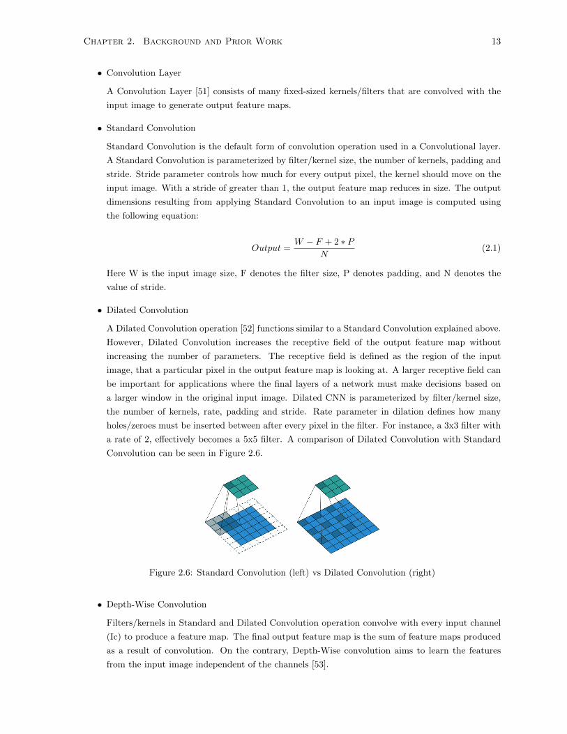
Recently, Convolutional Neural Networks (CNN) [48] have proven to be more robust to visual ap-

pearance variations than conventional neural networks. Before discussing the use of CNN’s in gaze

estimation systems, we first give a brief description of some of the common elements of a CNN image

processing pipeline since we employ such networks even for our feature extractor.

Convolutional Neural Networks Convolutional Neural networks (CNN’s) are artificial neural net-

works optimized to find the spatial relationship in data [48]. They are explicitly used in computer

vision for classification, regression, segmentation and object detection tasks [49, 50]. A typical CNN

architecture consists of several types of computational layer. Each computation layer consists of con-

volutional layers, pooling layers and batch normalization. Convolution operation used in convolutional

layers can itself be of different forms, including Standard Convolution, Depth-Wise Convolution, Dilated

Convolution and Transposed Convolution.

Other essential elements of a CNN include optimization algorithm, loss function, weight initialization

and activation function. Each of these elements is discussed in detail.


• Convolution Layer

A Convolution Layer [51] consists of many fixed-sized kernels/filters that are convolved with the

input image to generate output feature maps.

• Standard Convolution

Standard Convolution is the default form of convolution operation used in a Convolutional layer.

A Standard Convolution is parameterized by filter/kernel size, the number of kernels, padding and

stride. Stride parameter controls how much for every output pixel, the kernel should move on the

input image. With a stride of greater than 1, the output feature map reduces in size. The output

dimensions resulting from applying Standard Convolution to an input image is computed using

the following equation:

Output =W − F + 2 ∗ P

N(2.1)

Here W is the input image size, F denotes the filter size, P denotes padding, and N denotes the

value of stride.

• Dilated Convolution

A Dilated Convolution operation [52] functions similar to a Standard Convolution explained above.

However, Dilated Convolution increases the receptive field of the output feature map without

increasing the number of parameters. The receptive field is defined as the region of the input

image, that a particular pixel in the output feature map is looking at. A larger receptive field can

be important for applications where the final layers of a network must make decisions based on

a larger window in the original input image. Dilated CNN is parameterized by filter/kernel size,

the number of kernels, rate, padding and stride. Rate parameter in dilation defines how many

holes/zeroes must be inserted between after every pixel in the filter. For instance, a 3x3 filter with

a rate of 2, effectively becomes a 5x5 filter. A comparison of Dilated Convolution with Standard

Convolution can be seen in Figure 2.6.

Figure 2.6: Standard Convolution (left) vs Dilated Convolution (right)

• Depth-Wise Convolution

Filters/kernels in Standard and Dilated Convolution operation convolve with every input channel

(Ic) to produce a feature map. The final output feature map is the sum of feature maps produced

as a result of convolution. On the contrary, Depth-Wise convolution aims to learn the features

from the input image independent of the channels [53].


Depth-Wise Convolution is parameterized by kernel size, stride, padding, and channel multiplier

(Cm). The parameter Cm decides how many input channels a kernel should convolve with. In

Figure 2.7, Cm is set to a value of 1. The number of channels in the output of a Depth-Wise convo-

lution operation is equivalent to Ic*Cm. The output of Depth-Wise Convolution is usually followed

by a pointwise (1x1) Standard Convolution operation to average out the channel’s information.

Figure 2.7: Depth-Wise Convolution followed by 1x1 Standard Convolution

• Transposed Convolution

Transposed Convolution, also known as deconvolution [54], is parameterized by the number of

kernels, kernel size, padding and stride. Transposed Convolution is used to increase the resolution

of the input image. For every pixel in the input image, a kernel in a Transposed Convolution

strides over the output feature map. The value of stride is usually higher than 1.

The kernel values get multiplied with the corresponding input pixel. The resulting weighted kernel

values get copied to the overlapping region in the output feature map. An illustration of how

transposed convolution works can be seen in Figure 2.8. Here an input image of 2x2 is upsampled

to a feature map of size 4x4.

Figure 2.8: Upsampling using Transposed CNN

• Pooling Layer

Pooling layers also reduce the size of the feature maps [55]. They are generally used after a

convolutional layer. These layers typically reduce the size using averaging neighbouring elements

or selecting the maximum value within a local window. Pooling increases the receptive field of a

neuron, increasing the network’s performance for some tasks.


• Batch Normalisation

Batch normalization normalizes the output feature maps of the hidden layers in a CNN network

[56]. Batch normalization has a regularization effect, which can reduce overfitting and improves

generalization.

• Activation Function

An activation function introduces non-linearity into the output of the system. Many different

activation functions are used in neural networks, with some of the popular ones being Sigmoid,

Rectifier Linear Unit (ReLU) and Tanh.

Sigmoid and Tanh are usually used at the output layer of the network. The range of the tanh

function is [-1,1] and that of the sigmoid function is [0,1].

ReLU activation function [57] is the most widely used activation function in the hidden layers of

a neural network. This function is computationally faster than Sigmoid and Tanh and allows the

network to train faster.

• Optimization Algorithm

The optimization algorithm defines how the trainable parameters should be updated to minimize

the loss function. Gradient descent is the most commonly used optimization algorithm in which

parameters are updated in the negative gradient direction. The amount of step taken in this

direction is determined by a hyperparameter called the learning rate. To ensure minimization is

achieved quickly, Gradient descent with momentum adds velocity in the negative gradient direction

by using the previously computed gradients [58].

The more recent self-learning optimization algorithms, such as Adam [59], have momentum and

varying learning rates for each of the parameters depending on the gradient’s value. For instance,

smaller gradients require more significant learning rates while larger gradient requires small learning

rates for faster minimization.

• Initialisation Parameters

An initialization function defines how to set a neural network’s weights before the first training step

occurs. Standard options include uniform random or Gaussian distributions. Popular initialisations

used across neural networks is proposed by He and Xavier [60] which use Gaussian distributions

with zero mean and variance that is proportional to the inverse of the number of weights of each

layer.

The use of CNN’s for gaze estimation in head-mounted systems is seen in [1, 32]. The methods

described in [1, 32] addressed the issues of large training data requirements by making use of synthetic

eye images. Synthetic eye images allow these systems to model varying illumination effects, camera,

and eye pose under different gaze directions [61, 62]. In [1], authors train a CNN using 240K synthetic

eye images from ten synthetic subjects and 15K images from three real people to determine the gaze

direction in 3D inside an AR and VR headsets. The authors also generated synthetic eye images under

device slippage by moving the synthetic eye model by a small random offset. When the system was

tested on images of seven real people (approximately 7500 images), with targets displayed on a fixed

plane in the 3D scene, the mean accuracy was 2.1◦.


A different approach of using a CNN to estimate gaze direction is described in [32]. Here a hierarchy

of CNN networks is used to emulate every step of 3D model-based eye tracking is proposed, based on the

model approach of [26]. Eye images from 600 people were collected inside an MR headset while subjects

were looking at target points in a 3x3 grid at six different fixation distances. The authors ensured that

as the fixation distance varies, the target points are updated such that the gaze direction remains the

same. Testing on 160 people resulted in an average gaze accuracy of 3◦.

Appearance-based systems are promising but require extensive training datasets and are less accurate

than feature-based and model-based approaches. There are also limited reports on the effect of device

motion on system performance.

We have now discussed all the various gaze estimation methods. From the discussed approaches,

the model-based approach [26] is the only method that satisfies the fundamental requirements of an eye

tracking system for head-mounted XR systems (discussed in Chapter 1). A prerequisite in using the 3D

gaze estimation model [26] is the accurate estimation of eye features. These eye features are the centers

of the pupil and corneal reflections. Also, matching between the corneal reflections and its corresponding

light sources must be known. In the next section, we summarize the state-of-the-art feature extraction

methods for pupil center estimation, corneal reflection detection and corresponding matching.

2.2.4 Feature Extraction Methods

One key to the success of the 3D model-based eye tracking is the accuracy of the eye features extracted

from the eye images, particularly locating the center of the pupil and a very accurate location of the

corneal reflections along with finding its correspondence with a light source. In this section, we review

prior works in these areas.

Pupil Center Estimation

A pupil is said to be detected if the Euclidean distance between the actual pupil center and the estimated

pupil center is less than 5-pixels [63]. In contrast, a pupil center is estimated with high precision if the

distance between the actual pupil center and the estimated center is minimal. The 3D gaze estimation

model requires precise pupil center estimation.

However, in recent years, there has been considerable attention to pupil detection in IR head-mounted

eye tracking systems. This also has resulted in a wide variety of publicly available pupil detection datasets

[64, 65, 63, 66, 67]. These consist of IR eye images recorded in several challenging scenarios and have led

to the formulation of many pupil detection methods that are rule-based (the term we use for traditional

algorithmic approaches) [65, 64, 68, 69] as well as based on deep learning [1, 70]. Example images for

some of these datasets, including an image from our system, can be seen in Figure 2.9. Before we discuss

the state-of-the-art methodologies for pupil center estimation, we next provide an outline for the pupil

detection approaches.

Rule-based pupil detection algorithms for IR head-mounted eye tracking systems include Ellipse

Selection (ElSe) [64], Exclusive Curve Selector (ExCuSe)[65], Pupil Reconstructor (PuRe) [68], and

Pupil Reconstructor with Subsequent Tracking (PuReST) [69]. Both ELSe and ExCuSe consist of two

approaches for finding a pupil. Their main approaches use canny edge detector to find the edges in the

image, followed by edge filtering and finally fitting an ellipse to the edges which belong to the pupil.

Similarly, PuRe starts with morphological edge filtering, followed by each curved edge segment scoring


based on the likelihood that it belongs to a pupil. Scoring is done based on the ellipse aspect ratio,

angular spread of edges, among other factors. Finally, edge segments with high scores are combined to

form the pupil boundary.

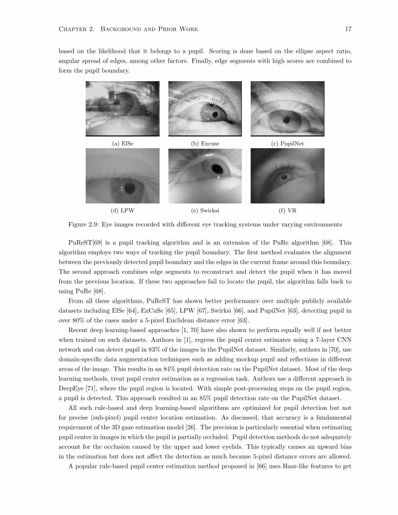
(a) ElSe (b) Excuse (c) PupilNet

(d) LPW (e) Swirksi (f) VR

Figure 2.9: Eye images recorded with different eye tracking systems under varying environments

PuReST[69] is a pupil tracking algorithm and is an extension of the PuRe algorithm [68]. This

algorithm employs two ways of tracking the pupil boundary. The first method evaluates the alignment

between the previously detected pupil boundary and the edges in the current frame around this boundary.

The second approach combines edge segments to reconstruct and detect the pupil when it has moved

from the previous location. If these two approaches fail to locate the pupil, the algorithm falls back to

using PuRe [68].

From all these algorithms, PuReST has shown better performance over multiple publicly available

datasets including ElSe [64], ExCuSe [65], LPW [67], Swirksi [66], and PupilNet [63], detecting pupil in

over 80% of the cases under a 5-pixel Euclidean distance error [63].

Recent deep learning-based approaches [1, 70] have also shown to perform equally well if not better

when trained on such datasets. Authors in [1], regress the pupil center estimates using a 7-layer CNN

network and can detect pupil in 83% of the images in the PupilNet dataset. Similarly, authors in [70], use

domain-specific data augmentation techniques such as adding mockup pupil and reflections in different

areas of the image. This results in an 84% pupil detection rate on the PupilNet dataset. Most of the deep

learning methods, treat pupil center estimation as a regression task. Authors use a different approach in

DeepEye [71], where the pupil region is located. With simple post-processing steps on the pupil region,

a pupil is detected. This approach resulted in an 85% pupil detection rate on the PupilNet dataset.

All such rule-based and deep learning-based algorithms are optimized for pupil detection but not

for precise (sub-pixel) pupil center location estimation. As discussed, that accuracy is a fundamental

requirement of the 3D gaze estimation model [26]. The precision is particularly essential when estimating

pupil center in images in which the pupil is partially occluded. Pupil detection methods do not adequately

account for the occlusion caused by the upper and lower eyelids. This typically causes an upward bias

in the estimation but does not affect the detection as much because 5-pixel distance errors are allowed.

A popular rule-based pupil center estimation method proposed in [66] uses Haar-like features to get


a rough estimate of the pupil. K means clustering on the intensity histogram around the course pupil

estimate followed by modified RANSAC ellipse fitting is used to estimate the pupil boundary. Pupil

Labs, a commercial eye tracking company, employs a similar approach to get a rough estimate of the

pupil followed by edge filtering [38]. The dark region in the eye image is then estimated using the

intensity histogram and user-defined threshold. The edges corresponding to this dark region is used to

find the pupil boundary.

Deep learning for pupil center estimation in head-mounted systems has also been previously used

[32], where multiple CNNs were employed. This work achieved an average Euclidean distance error of 0.7

pixels (on images with a resolution of 160 x 120 pixels). Another approach used a CNN-based regression

model [72], (with a wearable IR camera was attached to the user’s head) and achieved a mean Euclidean

distance error of 1 pixel on 120x80 resolution images.

In our work, we show that the pupil center in head-mounted VR systems can be estimated with high

precision under varying scenarios using a deep-learning-based semantic segmentation approach. Using

our method, we show that our model can also detect pupil with accuracy comparable to new rule-based

and deep learning-based solutions on some of the challenging head-mounted IR datasets.

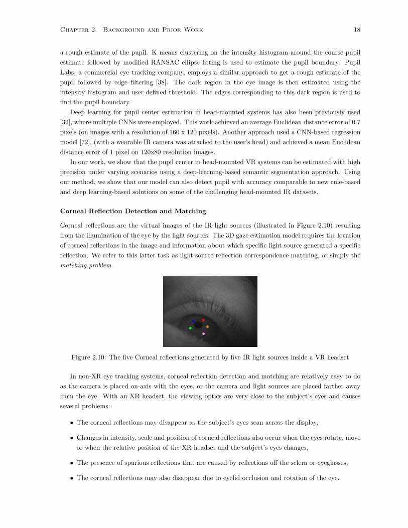
Corneal Reflection Detection and Matching

Corneal reflections are the virtual images of the IR light sources (illustrated in Figure 2.10) resulting

from the illumination of the eye by the light sources. The 3D gaze estimation model requires the location

of corneal reflections in the image and information about which specific light source generated a specific

reflection. We refer to this latter task as light source-reflection correspondence matching, or simply the

matching problem.

Figure 2.10: The five Corneal reflections generated by five IR light sources inside a VR headset

In non-XR eye tracking systems, corneal reflection detection and matching are relatively easy to do

as the camera is placed on-axis with the eyes, or the camera and light sources are placed farther away

from the eye. With an XR headset, the viewing optics are very close to the subject’s eyes and causes

several problems:

• The corneal reflections may disappear as the subject’s eyes scan across the display,

• Changes in intensity, scale and position of corneal reflections also occur when the eyes rotate, move

or when the relative position of the XR headset and the subject’s eyes changes,

• The presence of spurious reflections that are caused by reflections off the sclera or eyeglasses,

• The corneal reflections may also disappear due to eyelid occlusion and rotation of the eye.


State-of-the-art methodologies for detecting two or more corneal reflections and solving the matching

problem use rule-based and deep learning-based techniques.

Rule-based methods are designed for non-XR systems. The work in [73] uses a pattern of nine

light sources, and a corneal reflection is matched if it falls within the specified square in the 3x3 grid.

However, this method is unable to differentiate between a spurious and real corneal reflection. Another

approach [74] employs pattern matching to identify and find the correspondence between four corneal

reflections and four light sources. This method cannot compensate for the scaling of corneal reflections

due to changing Z distance between the eye tracker and the head and can only compensate for X/Y

translational movements. This method also assumes that the reflection closest to the pupil is a “true”

corneal reflection, which is a problem when there are spurious reflections present. Another approach

presented in [75] can track four corneal reflections based on a multivalued threshold algorithm, but

spurious reflections mislead this method. In [76], a homography-based approach is used to identify

corneal reflection patterns. It finds sub-patterns of corneal reflections accurately; however, the capacity

to compensate for translation and scaling effects is reduced when some corneal reflections are not present.

Also, this method requires the tuning of a scaling factor.

There is only one prior use of a CNN to solve the corneal reflection detection and the matching

problem described in [32]. In this approach, the authors use a hierarchy of three CNN networks to

detect and match four corneal reflections inside an XR system. The base architecture of the proposed

network is a RESNET-50 [77] network with feature pyramid outputs [78]. The base network output

is passed to two networks, one for matching corneal reflections with its light source and another for

corneal reflection localization. The localization accuracy reported by this system is under one pixel for

all four corneal reflections (in an image with resolution 160x120). The classification accuracy achieved

in matching a corneal reflection with its light sources is, on average, 96%. However, the authors fail to

report the accuracy to track corneal reflection’s patterns when some of the reflections are missing in the

images. Also, it is unclear how spurious reflections from the sclera or eyeglasses affect the accuracy of

the system.

Our work shows that by using just one CNN network, we can achieve similar accuracy and precision

of localization and correspondence matching under varying experimental conditions. The next chapter

discusses the software architecture of our end-to-end eye tracking system.

Chapter 3

End-to-End Eye Tracking Software

System

In this chapter, we present the software design of the end-to-end eye tracking system. The eye tracking

hardware module [31] used in our system was described in Chapter 2.

The top-level end-to-end software architecture for our eye tracking system is shown in Figure 3.1.

The Unity 3D virtual world generator provides the central control of the software system. Upon receiving

eye images from the left and right cameras (this operation is controlled by Pupil Capture application)

the Unity 3D engine passes this information to the eye tracking algorithm. The eye tracking algorithm

extracts eye features from the eye images (pupil and corneal reflection locations) and computes the gaze

direction using the 3D gaze estimation model. After receiving the computed gaze direction vector, the

Unity 3D engine draws this vector in the 3D scene. The point where the 3D gaze vector intersects with

a GameObject is the point-of-gaze. Unity 3D engine visualizes the computed point-of-gaze by rendering

a visual marker at the gaze position in the 3D scene. It also sends the point-of-gaze information to a

python based plotting application to display eye movements in real-time.

Figure 3.1: Software Architecture

This chapter describes the software blocks as mentioned in Figure 3.1, starting with the Pupil Capture

application.

20

Chapter 3. End-to-End Eye Tracking Software System 21

3.1 Pupil Capture Application

The Pupil Capture application is an open-source eye tracking application provided by Pupil Labs [31].

Pupil Capture provides the necessary USB video class device (UVC) interface with the cameras present

in the eye tracking hardware module. In addition to configuring the camera settings such as resolution

and frame rate, Pupil Capture allows accessing real-time video stream from the eye cameras. An interface

between the Unity 3D engine and Pupil Capture is provided by Pupil Labs [31].

Unity 3D engine generates the 3D scene with which a user interacts with. In the next section, we

describe the 3D scene used in our work.

3.2 3D scene for Calibration/Testing

The 3D scene used in our eye tracking system consists of a virtual camera, directional light source and

a 3D sphere.

• Virtual Camera: A virtual camera is an important component of a 3D scene. Recall from the

previous chapter, the 3D objects that fall within the FOV of the virtual camera, are visible to the

user. The VR headset’s head tracker controls the position and orientation of the virtual camera.

• Light Source : To ensure the 3D scene is properly illuminated we use a directional light source.

Illumination levels of a scene can be changed by changing the position and orientation of this light

source.

• 3D sphere: The 3D sphere is the target at which the user is instructed to gaze during the calibra-

tion/testing phase of our eye tracking system.

In the next section, we discuss the software components of our eye tracking algorithm in detail.

3.3 Eye Tracking Algorithm

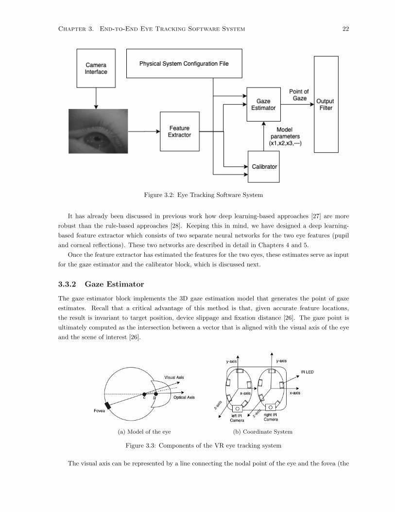
The top-level software architecture for our eye tracking algorithm is shown in Figure 3.2. This system

is attached to each of the two eyes. The output from both eyes is subsequently passed to a filter that

computes the final gaze estimate based on each eye’s estimates. The key software components are the

feature extractor (which determines the locations of the pupil centre and corneal reflections, and the

gaze estimator (which computes the point of gaze on the screen given the eye-features). For these to

work well with specific individuals, the system must be calibrated to each individual using the calibrator.

The three software components of our eye tracking algorithm are described in detail in the following

sections.

3.3.1 Feature Extractor

The feature Extractor block in our end-to-end eye tracking system is responsible for extracting eye

features from the images recorded using the left and right eye cameras. These features include the

pupil center, corneal reflections locations and their correspondence with the light sources. The 3D gaze

estimation model requires the locations of the center of the pupil and at least two corneal reflections in

the image of the eye to estimate the point of gaze [26].


Figure 3.2: Eye Tracking Software System

It has already been discussed in previous work how deep learning-based approaches [27] are more

robust than the rule-based approaches [28]. Keeping this in mind, we have designed a deep learning-

based feature extractor which consists of two separate neural networks for the two eye features (pupil

and corneal reflections). These two networks are described in detail in Chapters 4 and 5.

Once the feature extractor has estimated the features for the two eyes, these estimates serve as input

for the gaze estimator and the calibrator block, which is discussed next.

3.3.2 Gaze Estimator

The gaze estimator block implements the 3D gaze estimation model that generates the point of gaze

estimates. Recall that a critical advantage of this method is that, given accurate feature locations,

the result is invariant to target position, device slippage and fixation distance [26]. The gaze point is

ultimately computed as the intersection between a vector that is aligned with the visual axis of the eye

and the scene of interest [26].

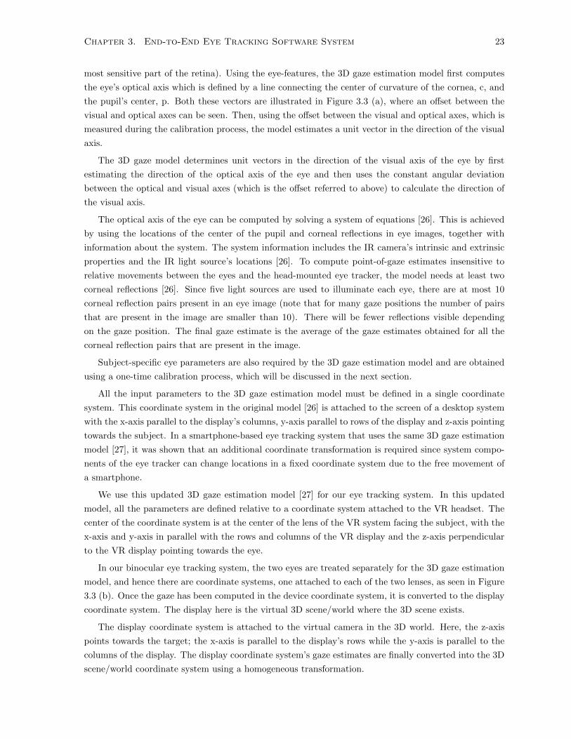
(a) Model of the eye (b) Coordinate System

Figure 3.3: Components of the VR eye tracking system

The visual axis can be represented by a line connecting the nodal point of the eye and the fovea (the


most sensitive part of the retina). Using the eye-features, the 3D gaze estimation model first computes

the eye’s optical axis which is defined by a line connecting the center of curvature of the cornea, c, and

the pupil’s center, p. Both these vectors are illustrated in Figure 3.3 (a), where an offset between the

visual and optical axes can be seen. Then, using the offset between the visual and optical axes, which is

measured during the calibration process, the model estimates a unit vector in the direction of the visual

axis.

The 3D gaze model determines unit vectors in the direction of the visual axis of the eye by first

estimating the direction of the optical axis of the eye and then uses the constant angular deviation

between the optical and visual axes (which is the offset referred to above) to calculate the direction of

the visual axis.

The optical axis of the eye can be computed by solving a system of equations [26]. This is achieved

by using the locations of the center of the pupil and corneal reflections in eye images, together with

information about the system. The system information includes the IR camera’s intrinsic and extrinsic

properties and the IR light source’s locations [26]. To compute point-of-gaze estimates insensitive to

relative movements between the eyes and the head-mounted eye tracker, the model needs at least two

corneal reflections [26]. Since five light sources are used to illuminate each eye, there are at most 10

corneal reflection pairs present in an eye image (note that for many gaze positions the number of pairs

that are present in the image are smaller than 10). There will be fewer reflections visible depending

on the gaze position. The final gaze estimate is the average of the gaze estimates obtained for all the

corneal reflection pairs that are present in the image.

Subject-specific eye parameters are also required by the 3D gaze estimation model and are obtained

using a one-time calibration process, which will be discussed in the next section.

All the input parameters to the 3D gaze estimation model must be defined in a single coordinate

system. This coordinate system in the original model [26] is attached to the screen of a desktop system

with the x-axis parallel to the display’s columns, y-axis parallel to rows of the display and z-axis pointing

towards the subject. In a smartphone-based eye tracking system that uses the same 3D gaze estimation

model [27], it was shown that an additional coordinate transformation is required since system compo-

nents of the eye tracker can change locations in a fixed coordinate system due to the free movement of

a smartphone.

We use this updated 3D gaze estimation model [27] for our eye tracking system. In this updated

model, all the parameters are defined relative to a coordinate system attached to the VR headset. The

center of the coordinate system is at the center of the lens of the VR system facing the subject, with the

x-axis and y-axis in parallel with the rows and columns of the VR display and the z-axis perpendicular

to the VR display pointing towards the eye.

In our binocular eye tracking system, the two eyes are treated separately for the 3D gaze estimation

model, and hence there are coordinate systems, one attached to each of the two lenses, as seen in Figure

3.3 (b). Once the gaze has been computed in the device coordinate system, it is converted to the display

coordinate system. The display here is the virtual 3D scene/world where the 3D scene exists.

The display coordinate system is attached to the virtual camera in the 3D world. Here, the z-axis

points towards the target; the x-axis is parallel to the display’s rows while the y-axis is parallel to the

columns of the display. The display coordinate system’s gaze estimates are finally converted into the 3D

scene/world coordinate system using a homogeneous transformation.


3.3.3 Calibrator

The calibrator estimates subject-specific eye properties. These properties are used by the 3D gaze

estimation model to estimate the unit vector in the direction of the visual axis. For each eye three

parameters are derived during the calibration process. These parameters are saved and can be used

later to estimate the gaze position of the same subject (i.e., each subject requires only one calibration

procedure). The calibration procedure include the following stages:

Data Collection – In this stage, the calibration routine displays several gaze targets at ± 5◦ field

of view one at a time at fixed fixation distance on the VR screen (Figure 3.4). This fixation distance

can be at various distances in the 3D world, but one has to ensure that the target is visible in the 3D

scene. For our system, we selected a fixation distance of 1m and a target in a shape of a sphere with a

radius of 2.5 cm (i.e., the sphere subtends a solid angle of approximately ±1.4◦ to the eye).The subject

is instructed to gaze at the middle of the target while the feature extractor estimates the pupil center

and corneal reflections at each target position (50 estimates at each position). Once completed, the

calibration target moves to the next location. Our calibration routine has nine target positions.

Figure 3.4: The calibration points at ±5◦are denoted by color red. Blue (±10◦) and green color points(±15◦) are the test points that will be used to evaluate the system.

Outlier Removal – This stage identifies which eye features collected in the previous stage are inac-

curate and discarded. The first step is to initialize the three subject-specific eye parameters estimated

during the calibration routine to the average expected human values. Then for each of the eye features

collected from the previous step, a point of gaze is determined. Outliers are gaze estimates that are

located two or more standard deviations away from that target’s mean.

Parameter Optimization – A non-convex optimization process minimizes the sum of squared Eu-

clidean distances between the known calibration targets and the calculated gaze locations, by varying

the calibration parameters in Table 3.1.

The last two steps (outlier removal and parameter optimization) of the calibration processes are

repeated for every pair of corneal reflections in the eye images and a different set of calibration parameters

is computed for every corneal reflection pair. The unique set of parameters that is computed for each

pair of corneal reflections is used by the gaze-estimation module when this pair is used for the estimation

of the gaze vector. In a later section, we describe how we select the corneal reflections used for gaze

estimation.

The gaze estimator and calibrator modules are based on software that was developed for a smartphone-


Name Description valueK Distance between center of corneal curvature and center of pupil mm

Alpha Horizontal angle between optical and visual axis degreesBeta Vertical angle between optical and visual axis degrees

Table 3.1: Calibration Parameters

based eye tracking system [27]. Minor modifications were required to accommodate changes between

the two systems. An interface which allow the eye tracking algorithm for the two eyes to be executed in

parallel was also created.

3.4 Physical System Configuration

The 3D gaze estimation model requires information about the optical and geometrical properties of the

eye-tracking system. The system properties include the locations of light sources and cameras, and the

camera’s intrinsic parameters (see Table 3.2). As described in a previous section, all the parameters

are defined relative to the device coordinate system, which in our case is attached to the VR lens. The

center of the VR lens acts as the origin of the device coordinate system. The camera and light source’s

physical locations relative to the lens’s center were measured with a caliper and the the cameras’ yaw,

pitch, and roll angles relative to orientation of the lens with a protractor.

Param Description UnitsCamera Focal Length Distance between the nodal point of lens and image sensor mmCamera Resolution Resolution of camera sensor pixels

Camera Principal Point Location of intersection of the optical axis on the image sensor pixels

Camera Location X Y Z location of the principal point mm

Camera Pixel X Y Z location of the principal point mm

Camera Orientation Rotation about the x,y and z axis mm

Infrared LED locations X,Y and Z locations of the two infrared light sources mm

Table 3.2: Physical System Parameters

We have now discussed the major blocks of our eye tracking algorithm. In the next section, we

discuss the final step in our eye tracking system which is the visualisation of gaze estimates.

3.5 Gaze Visualisation

Once the Unity 3D engine receives a gaze vector from the eye tracking algorithm, this gaze vector is

drawn in the 3D scene. The point in the 3D scene, where the gaze vector intersects with a GameObject

is the point-of-gaze. To visualise the point-of-gaze, a visual marker is created in the 3D scene. Another

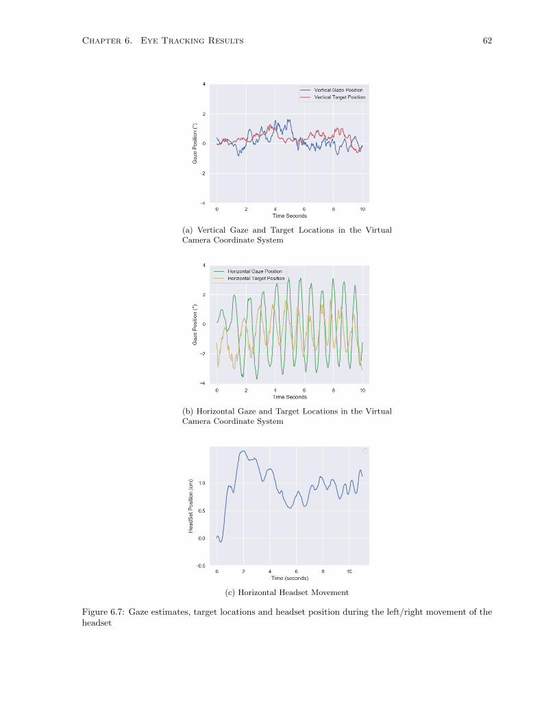
method to visualise gaze estimates is by plotting gaze in real-time. Plotting gaze estimates over time

(time-chart) support viewing of eye movements traces. This helps in understanding how eye movements

change with changing target position.

We have now described all the major blocks of the end-to-end eye tracking system. In the next


two chapters, we describe the two eye feature estimation networks that are part of the feature extrac-

tor: pupil center and corneal reflections. We also compare the proposed networks with state-of-the-art

methodologies.

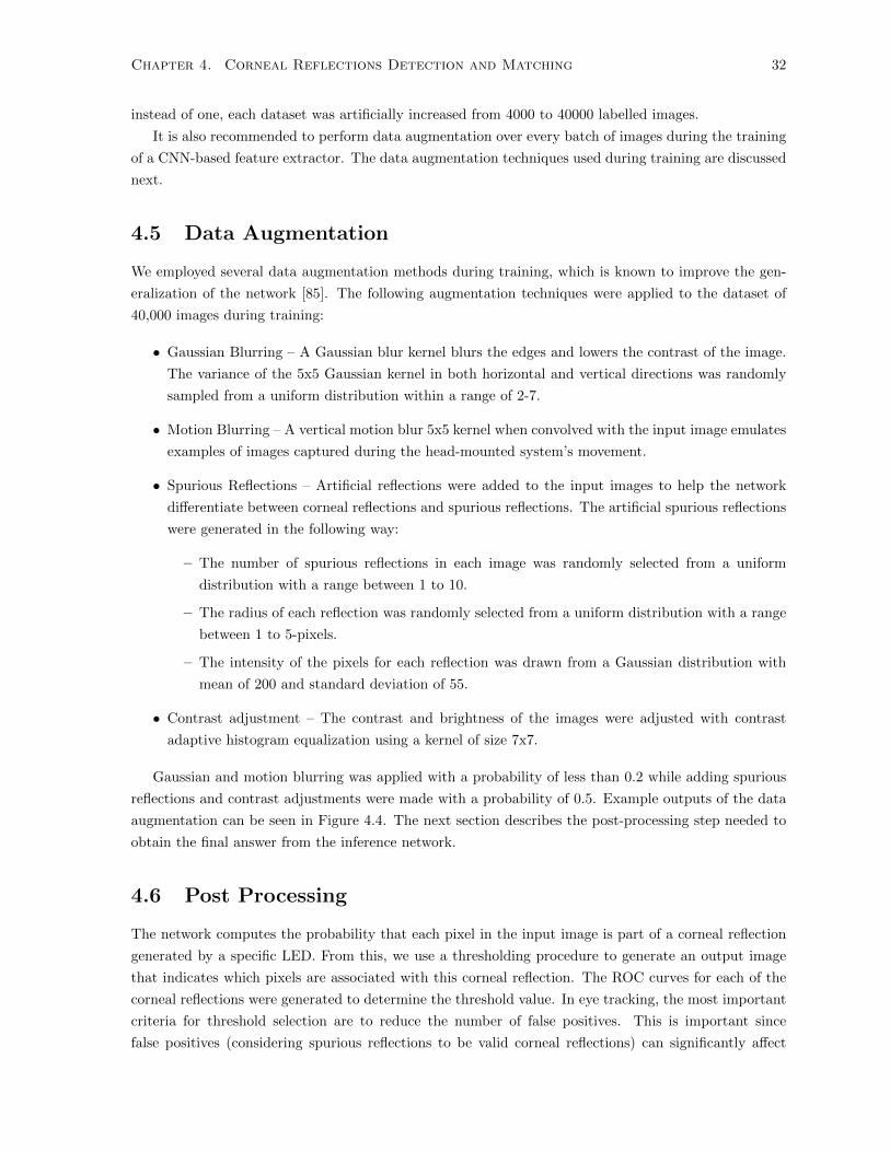
Chapter 4

Corneal Reflections Detection and

Matching

Corneal reflections are the virtual images of the IR light sources on the cornea. The coordinates of two

or more corneal reflections along with information about the correspondence with their light source is

required by the 3D gaze estimation model to calculate gaze direction [26].

Our eye tracking system has five light sources per eye, which results in five corneal reflections. The use

of five light sources introduces a difficult problem: the need to match each of the five corneal reflections

with the corresponding light source over the range of expected eye movements. In Chapters 1 and 2, we

have already discussed the challenges associated with corneal reflection detection and matching in XR

systems. We also described the reasons why solving this problem is relatively easier to do in non-XR

systems.

The focus of this chapter is to introduce a new method to locate corneal reflections and determine

the correct matching to their corresponding light sources in an XR system. These steps are essential to

successful eye tracking XR systems.

State-of-the-art methodologies discussed in Chapter 2 for solving the detection and matching of

more than two corneal reflections include rule-based and deep learning-based methods. While rule-

based methods are designed for non-XR systems, only one prior use of a CNN to solve the corneal

reflection detection and the matching problem is described in [32] for an XR system. In this approach,

the authors use a hierarchy of three CNN networks to detect and match four corneal reflections. The

base architecture of the proposed network is a RESNET-50 [77] network with feature pyramid outputs

[78]. The base network’s output is passed to two networks, one for matching corneal reflections with its

light source and another for corneal reflection localization.

By contrast, in our approach, we perform localization and classification of corneal reflections within

a single network, using semantic segmentation [79]. One of the most popular architectures for semantic

segmentation in biomedical applications is UNET [29], which has been recently used to locate the pupil

and iris regions within eye images [80, 81]. We use a UNET-style architecture to locate the corneal

reflections present in the image and solve the corneal reflection-LED correspondence matching problem.

To our knowledge, this is a novel solution to the correspondence matching problem.

Our proposed system takes input an image of the eye region of size 320x240 pixels (downsampled

from the original image of size 640x480). The system’s output is five probability maps also of size

27

Chapter 4. Corneal Reflections Detection and Matching 28

320x240 with one map for each of the five corneal reflections. Each of the five maps represents the

probability that a pixel in the original image is part of a corneal reflection generated by one of the five

light sources. To train the network, labels of the same size as that of input are generated. Each pixel in

the label images is encoded as 1 or 0, depending on whether it belongs to a corneal reflection. A detailed

discussion of the data labelling procedure is given in Section 4.3. Since the labels have an encoding of

0’s and 1’s, we also refer to them as binary masks.

4.1 Network Architecture

Our system’s architecture is based on the UNET architecture described in [29]. The UNET architecture

as seen in Figure 4.1 is symmetric and consists of two major parts — a contracting path constituted by

the general convolutional process for learning features at different resolutions; the expansive path, which

is constituted by upsampling and convolutional layers to produce an output of the same size as input.

Input and Output share the same size since UNET performs pixel-wise classification, also known

as semantic segmentation [79]. The information in the downscaled feature map is concatenated with

the upsampled feature map (also known as skip connection). Concatenation is done to ensure that

the networks learn the information it needs for feature estimation and understand the learned feature’s

spatial locations in the original image.

Figure 4.1: UNET Style Architecture

In the next section, we will discuss the objective function used to train such a network.

4.1.1 Objective Function

Our goal is to find the five regions in the image that correspond to the five corneal reflections. To train

the network, we use an equally weighted combination of Cross-Entropy (CE) [82] and the Soft Dice loss

[83] as the objective function that we now discuss in detail.

CE loss measures the divergence between the ground truth (manually labelled) and the prediction for

each pixel in the image [82]. Our network’s goal is to find the five regions in the image that correspond

to the five corneal reflections. As a result, the divergence between prediction and label across each pixel

for all five regions is first computed and then is averaged across all the regions.


Let the number of pixels in the image be P where p ( P , the number of corneal reflection regions as

S (== 5 in our case) where s ( S, the pixel value in the binary mask l, and the prediction pixel value

r. Then the CE loss for a single image can be represented as:

CE =1

S

S∑s=1

p∑p=1

lsp ∗ log(rsp) (4.1)

This objective function is insufficient because the number of pixels belonging to the region where

the corneal reflections exist is much less than the number of background pixels. Thus, the CE loss

function has a bias to predict that a pixel is part of the background, rather than the corneal reflection.

A common way to overcome this kind of imbalance is to use the Soft Dice loss function [83], which deals

with the problem of imbalance between target and background sizes without the need for explicit class

weighting. The Soft Dice loss function is differentiable and acts as a global operator since it operates

at the image-level compared to the CE loss, which works at the pixel level. The soft Dice coefficient is

computed across the five regions corresponding to each of the corneal reflections and is given by:

SoftDice = 1−∑s

s=1

∑pp=1 2 ∗ lsp ∗ rsp∑s

s=1

∑pp=1(lsp)2 + (rsp)2 + ε

(4.2)

A small value of epsilon (ε) is added to the denominator to handle the cases where the prediction

and label pixels contain only zeros, representing scenarios where no corneal reflection is present in the

image.

In the next section, we discuss how the model was trained, starting with data collection.

4.2 Data Collection

We collected eye images from 15 people using an eye tracking hardware module manufactured by Pupil

Labs [31] inside an HTC Vive VR headset [34]. This binocular eye tracking module includes an IR

camera and five IR light sources for each eye. The IR camera recorded images with a resolution of

640x480 pixels of both the left and right eyes while the subjects looked at targets on the VR display.

The screen’s targets spanned horizontal and vertical ranges of ± 15◦ of the Field of View (FOV). This

range ensured that many of the training examples were missing some of the corneal reflections due to

the light sources reflecting the sclera rather than the cornea or eyelid occlusion. Three subjects out of

the 15 were wearing glasses during the study.

Recognizing that this is a small (by subject count) dataset, we explored different ways of increasing

our dataset. We had looked for public datasets that were relevant, but typical eye feature estimation

datasets are meant for pupil/iris detection[63, 67, 84] and do not have the right number of corneal

reflections (our system requires images that have up to five corneal reflections, which is dependent on

our hardware system). One publicly available unlabelled dataset (from NVIDIA) [1] is collected using

hardware similar to what we are using in our system. In this dataset from NVIDIA, data, which contained

ten people, is available under various conditions (eyeglasses, contact lenses, and lighting conditions). We

added these ten people to our dataset and manually labelled the corneal reflections. Thus, in total, there

are 25 people in our dataset. The labelling methodology for this data is described next.


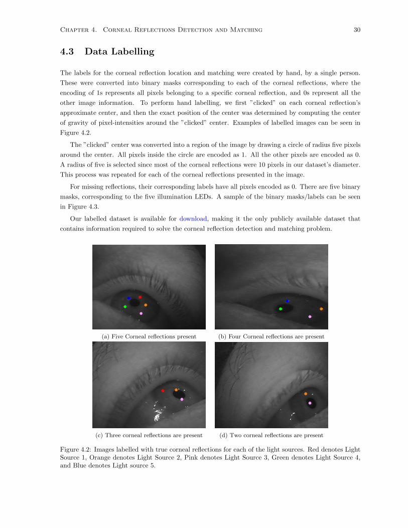
4.3 Data Labelling

The labels for the corneal reflection location and matching were created by hand, by a single person.

These were converted into binary masks corresponding to each of the corneal reflections, where the

encoding of 1s represents all pixels belonging to a specific corneal reflection, and 0s represent all the

other image information. To perform hand labelling, we first ”clicked” on each corneal reflection’s

approximate center, and then the exact position of the center was determined by computing the center

of gravity of pixel-intensities around the ”clicked” center. Examples of labelled images can be seen in

Figure 4.2.

The ”clicked” center was converted into a region of the image by drawing a circle of radius five pixels

around the center. All pixels inside the circle are encoded as 1. All the other pixels are encoded as 0.

A radius of five is selected since most of the corneal reflections were 10 pixels in our dataset’s diameter.

This process was repeated for each of the corneal reflections presented in the image.

For missing reflections, their corresponding labels have all pixels encoded as 0. There are five binary

masks, corresponding to the five illumination LEDs. A sample of the binary masks/labels can be seen

in Figure 4.3.

Our labelled dataset is available for download, making it the only publicly available dataset that

contains information required to solve the corneal reflection detection and matching problem.

(a) Five Corneal reflections present (b) Four Corneal reflections are present

(c) Three corneal reflections are present (d) Two corneal reflections are present

Figure 4.2: Images labelled with true corneal reflections for each of the light sources. Red denotes LightSource 1, Orange denotes Light Source 2, Pink denotes Light Source 3, Green denotes Light Source 4,and Blue denotes Light source 5.

https://www.eecg.utoronto.ca/~jayar/datasets/xreyetrack.html


(a) Corneal Reflection - Light Source 1 (b) Corneal Reflection - Light Source 2

(c) Corneal Reflection - Light Source 3 (d) Corneal Reflection- Light Source 4

(e) Corneal Reflection - Light Source 5

Figure 4.3: Binary Masks for each of the corneal reflections for the Labelled image in 4.2

4.4 Dataset Generation

A neural network is typically trained using a large dataset. Since labelling is a slow and time-consuming

step, one can speed up the processing by using the labelled information and generate new images. Our

labelled image is of size 640x480, while our feature extractor is designed to take an input image of

320x240. To increase the dataset and avoid labelling of more images, we use the labelled information

and generate ten fixed size crops of size 320x240 from 640x480. It is ensured that the pupil and all

corneal reflections are inside this crop. Each crop around the same eye location would vary the pupil

center’s relative placement within that window under the constraint that both corneal reflections and

the pupil must be contained in the windows for valid regions.

The ten specific crop locations were generated randomly from the set of all possible crop locations

for a specific eye region that meets these constraints. By taking ten fixed size crops per eye location


instead of one, each dataset was artificially increased from 4000 to 40000 labelled images.

It is also recommended to perform data augmentation over every batch of images during the training

of a CNN-based feature extractor. The data augmentation techniques used during training are discussed

next.

4.5 Data Augmentation

We employed several data augmentation methods during training, which is known to improve the gen-

eralization of the network [85]. The following augmentation techniques were applied to the dataset of

40,000 images during training:

• Gaussian Blurring – A Gaussian blur kernel blurs the edges and lowers the contrast of the image.

The variance of the 5x5 Gaussian kernel in both horizontal and vertical directions was randomly

sampled from a uniform distribution within a range of 2-7.

• Motion Blurring – A vertical motion blur 5x5 kernel when convolved with the input image emulates

examples of images captured during the head-mounted system’s movement.

• Spurious Reflections – Artificial reflections were added to the input images to help the network

differentiate between corneal reflections and spurious reflections. The artificial spurious reflections

were generated in the following way:

– The number of spurious reflections in each image was randomly selected from a uniform

distribution with a range between 1 to 10.

– The radius of each reflection was randomly selected from a uniform distribution with a range

between 1 to 5-pixels.

– The intensity of the pixels for each reflection was drawn from a Gaussian distribution with

mean of 200 and standard deviation of 55.

• Contrast adjustment – The contrast and brightness of the images were adjusted with contrast

adaptive histogram equalization using a kernel of size 7x7.

Gaussian and motion blurring was applied with a probability of less than 0.2 while adding spurious

reflections and contrast adjustments were made with a probability of 0.5. Example outputs of the data

augmentation can be seen in Figure 4.4. The next section describes the post-processing step needed to

obtain the final answer from the inference network.

4.6 Post Processing

The network computes the probability that each pixel in the input image is part of a corneal reflection

generated by a specific LED. From this, we use a thresholding procedure to generate an output image

that indicates which pixels are associated with this corneal reflection. The ROC curves for each of the

corneal reflections were generated to determine the threshold value. In eye tracking, the most important

criteria for threshold selection are to reduce the number of false positives. This is important since

false positives (considering spurious reflections to be valid corneal reflections) can significantly affect


(a) With spurious reflections (b) With all techniques applied

Figure 4.4: Images after data augmentation

errors in the gaze estimation. By contrast, a false negative only prevents the use of that reflection in

gaze computation (i.e., one can still use the other reflections). After determining the thresholds for

each corneal reflection such that a false positive rate is less than 0.2, the most significant connected

component in the image represents the corneal reflection, as shown in Figure 4.5.

If, after thresholding, no connected component is present in a specific map, it signifies that this specific

corneal reflection is missing from the image. Finally, the center of a corneal reflection is computed as

the center of mass of the probabilities across the X and Y-axes of the connected component.

(a) Raw Output from the network (b) Image after thresholding

Figure 4.5: Post-processing results for one of the corneal reflections

4.7 Artificial Spurious Reflections vs Real Corneal Reflections

Since we are not controlling the generated spurious reflection’s location, there can be cases where the

spurious reflections overlap with the true corneal reflections or their boundaries are touching. To dif-

ferentiate between the artificially generated spurious reflections and valid reflections, we computed the

Euclidean distance between the labelled corneal reflection centers and the predicted reflection. If the

Euclidean distance is greater than 5 pixels, then the predicted corneal reflection is considered spurious,

and the false-positive counter is incremented.

Until now, we have discussed all the steps involved in training a feature extractor. In the next section,

we discuss how the datasets for training, testing are generated.


4.8 Dataset Splitting

Three datasets, one for training, one for validation and one for testing were created from the generated

dataset of 40,000 images and 25 distinct subjects. The training data contained images from 19 different

people and used 76% of the available dataset. The remaining people were split equally between the

validation (12%) and test (12%) sets. We ensured that all the eye regions of any specific subject were

in one of these two subsets and not split between them. Subjects with eyeglasses were divided equally

among the three datasets, ensuring similar distribution across all three sets.

(a) Validation Dataset

(b) Test Dataset

Figure 4.6: Validation and Test Datasets Distribution based on the number of valid corneal reflectionspresent in the image

Both the test and the validation dataset consists of 4000 images each. Images in the test and

validation datasets represent the cases where three or more corneal reflections are present, as shown

in Figure 4.6. However, there are only a few instances where two or fewer reflections were present

since such scenarios mostly occur due to eyelid occlusion and blinking. Also, as a result of dividing the

dataset based on the number of people, we see a different distribution of images in the validation and

test datasets.

In the next section, we go deeper into the network architecture, starting with discussing the crucial


hyperparameters involved in this process.

4.9 Hyperparameter Tuning

The feature extraction network hyperparameters play an essential role in determining the accuracy and

real-time performance of the feature extraction system. As a common practice, the network is trained on

the training dataset, and the validation dataset is used to select the best values for the hyperparameters.

The test set is used to determine the final accuracy and performance metrics.

In tuning a network’s performance, we are concerned with both inference quality and the time required

to compute the inference. Low latency eye tracking is a fundamental requirement for eye tracking systems

in XR devices, especially for applications such as foveated rendering [25]. The work in [25] shows that

a gaze estimation rate above 25 frames/s is acceptable for foveated rendering. Our goal is to achieve a

gaze estimation rate of at least 30 frames/s cumulatively across the two feature estimation networks and

for both eyes running on a GPU available in VR enabled laptops (RTX 2060 in our case).

4.9.1 Specific Hyperparameters Explored

We have already described the corneal reflection detection and matching network’s overall structure,

which employs the UNET architecture [29]. This structure has two computation paths in sequential

order: a contracting path consisting of four downsampling blocks followed by an expansive path, con-

sisting of four upsampling blocks. Each of these blocks is a stack of two CNN layers with additional

downsampling and upsampling layers. Four hyperparameters arise in this global structure – the number

of blocks in the contracting and expansive paths (which must be equal), the number of CNN layers in

a block, the type of downsampling layer and the type of upsampling layer used. Because the original

architecture is too large and slow for the frame rates required in our system, we a priori restrict the

number of CNN layers per block to be one. However, the number of blocks was varied, as mentioned in

Table 4.1.

The choice of downsampling and upsampling layers is discussed next. Downsampling of the input

image can be achieved by either using a CNN layer with a stride greater than one or using a pooling

layer. In the case of upsampling, Transposed Convolution and Bilinear Interpolation are the two widely

used methods. Transposed Convolution [54] is a learnable convolution operation designed to learn the

pixel’s value that should be placed in the upsampled positions of the new image. A detailed explanation

can be seen in Chapter 2, Section 2.2.3. Bilinear interpolation [86] produces an upsampled feature map

by interpolating the new pixel’s value using its neighbouring pixels. We explored the combinations of

upsampling and downsampling layers, as listed in Table 4.1.

An influential design parameter for the CNN layers used in each of the blocks is the nature of the

convolution operation, as different approaches can significantly affect accuracy and computation time

[87]. We explored numerous alternatives between the three kinds of convolution, as listed in Table

4.1. These include Standard Convolution, Dilated Convolution, and Depth-Wise convolution. A detailed

explanation of the functioning of these convolution operations can be found in Chapter 2, Section 2.2.3.

The choice of convolution in CNN layers varied as a function of the type of block. This meant that

the CNN layers in upsampling blocks could use one of the three forms of convolution, while the CNN

layers in downsampling blocks could use either the same form of convolution as used in the upsampling

block or a different one.


Hyperparameter Possible ChoicesConvolution Type Standard, DepthWise, Dilated

Convolution Type used at which stage Upsampling, Downsampling, BothUpsampling Technique Bilinear Interpolation, Transposed Convolution

Downsampling Technique Strided Convolution, Max PoolingNumber of upsampling and downsampling blocks 3,4

Table 4.1: Hyperparameters Explored

Most of the hyperparameters discussed until now are further parameterized with at least 3-4 param-

eters. As discussed before, not all parameters were tuned because of limited resources and significant

training times of such networks. Table 4.2 presents the values for every possible value of the parameters

that were unchanged during hyperparameter tuning.

Hyperparameter ValuesKernel Size in CNN layers 3x3

Number of kernels in each CNN layer of the downsampling blocks For 4 blocks - 32, 64,128,256,For 3 blocks – 32,64,128

Rate when using dilation CNN (Nh) 2Channel multiplier when using depth wise CNN (Cm ) Strided Convolution, Max Pooling

Max Pooling Kernel Size 2x2Transposed CNN kernel size 2x2

Table 4.2: Unchanged Hyperparameters

4.10 Training/Exploration Process

The networks explored included Batch Normalization after every CNN layer [56] and used a ReLU

activation function [50]. The hyperparameters in Table 4.1 were explored by training each architecture

with the training dataset discussed above and measuring the quality of results on the validation set.

Training occurred for 120 epochs, with a batch size of 8 and a learning rate of 0.001. The network

was saved if the difference between validation and training loss showed no variation for five consecutive

epochs to permit early stopping. In training, we found that the Stochastic Gradient Descent (SGD)

with momentum [58] optimizer achieved a better generalization on the validation dataset compared to

self-adaptive optimizers [88].

We evaluate the trained networks on the validation dataset based on two metrics: the first metric

considers the accuracy which is defined as the proportion of all true corneal reflections that are found

and correctly matched with the originating light source.

The second metric, which was considered, is the computational cost of one forward inference through

the network. Precisely, this was measured as the inference time (in milliseconds), when running on

an RTX 2060 GPU. This value was determined by the neural network training’s profiler that we used

Tensorflow version 1.14 [89].

Appendix A presents the results for all the explored networks. Table 4.3 shows the results for the

networks that make use of max-pooling as the downsampling layer in the four downsampling blocks and


bilinear interpolations as the upsampling layer in the four upsampling blocks. These networks exhibit

higher accuracy than the rest of the explored networks.

From the list of possible networks presented in Table 4.3, the network that uses Dilated Convolution

in each of the CNN layers in the upsampling blocks and Standard Convolution in each of the CNN layers

in the downsampling blocks exhibits the best performance with a reported average accuracy of 95%.

This accuracy is 5% better than the network, which uses Standard Convolution in the upsampling and

downsampling blocks.

The use of dilated Convolution increases the inference time by 1.5 ms compared to the use of Standard

Convolution. However, even with increased inference time, the final network can still run at a frame

rate higher than 30 frames/sec, which is a requirement of our system.

Convolution Typein

Upsampling Blocks

Convolution Typein

Downsampling Blocks

CRDetection Rate (%)

InferenceTime(ms)

Dilated Dilated 93 6.5Standard Standard 90 4.2

Dilation Standard 95 5.7Standard Dilated 91 5.2

Depth-Wise Standard 91 4.7Depth-Wise Depth-Wise 90 4.5

Standard Depth-Wise 90 4.5

Table 4.3: Results for Corneal reflection Detection and Matching when max pooling used as downsam-pling with Biliner Interpolation as upsampling layer

To conclude, the selected corneal reflection network used the following hyperparameters:

• A Dilated Convolution is used in each of the CNN layers of the four upsampling blocks.

• A Standard Convolution is used in each of the CNN layers of the four downsampling blocks.

• Bilinear Interpolation is used as the upsampling layer.

• Max Pooling layer is used for downsampling.

Before discussing the performance of the final selected network on the test data set, it is required

to determine the threshold levels for each of the corneal reflections. This is an essential step in the

post-processing stage, as described in Section 4.6.

The threshold level for each corneal reflection is determined from the ROC curves (illustrated in

Figure 4.7), such that the false-positive rate is less than 0.2. A probability of 0.8 was determined to be

the threshold for each of the corneal reflections. A probability level of 0.8 corresponds to a grayscale

value of 200.

4.11 Corneal Reflection Detection and Matching Performance

on the Test Dataset

On the test dataset, our proposed network achieved an accuracy (defined in Section 4.10) of approxi-

mately 91%. This accuracy is reduced to 80% (as seen in 4.4) when tested on images which have only


Figure 4.7: ROC for each of the Corneal Reflections

two valid corneal reflections. The reduction of accuracy can be attributed to an increase in the mis-

classification due to incorrect matching, resulting in more false positives. When three or more corneal

reflections are present in the image, the average accuracy increased to 94%.

The confidence level of the network is evaluated using the Dice coefficient. The Dice coefficient [90]

measures the similarity between the label and the output. For perfect agreement between the generated

output and the prediction, this coefficient would be 1. The average Dice coefficient is 0.81 for images

where more than 3 corneal reflections are present. The coefficient drops by 3% when the number of valid

corneal reflections in the image decreases from 5 to 2 (as shown in Table 4.4). This indicates that the

network uses information associated with all corneal reflections (their relative position, pattern, etc.) to

solve the LED-reflection matching problem.

Valid Corneal reflections Accuracy (%) Dice Coefficient2 80.3 0.78

3-5 94.3 0.81

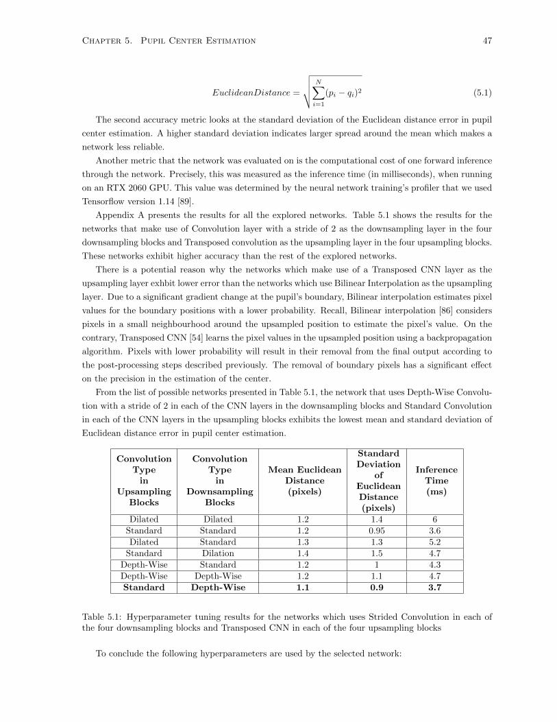
Table 4.4: Performance metrics based on number of valid reflections present in the image

In the next section, we compare our system’s performance with state-of-the-art rule-based and deep

learning methods.

4.12 Feature Extractor Performance Comparison with State-

of-the-art Methods

Existing rule-based approaches for corneal reflection detection and matching [74, 75, 76, 73] are designed

for non-XR systems. It is important to note that non-XR systems have far better images than XR systems

due to reasons described in the Chapter 1, Section 1.3. Therefore existing rule based approaches report a


relatively higher accuracy of 94% [73] compared to our system. However, this accuracy is not comparable

to the approaches designed for XR system due to the difference in the quality of the images.

The only previously-published approach designed for an XR system is based on deep learning [32].

The network in [32] reports an accuracy of 96%. However, our proposed network solves the more complex

problem of tracking five corneal reflections compared to the four in [32]. Also, our approach requires

1000 times less floating-point operations than [32] during inference.

It is hard to make a direct comparison between [32] and our network due to the lack of open-source

labelled datasets for corneal reflection detection and matching. However, we can compare the two

networks by evaluating the performance of the end-to-end eye tracking system, since both [32] and our

system makes use of corneal reflections for gaze estimation. The accuracy of the eye tracking system

will deteriorate if the performance of the corneal reflection detection and matching network (dependent

on the training dataset) is poor. A detailed comparison of these two eye tracking systems is given in

Chapter 6.

In the next section, we discuss the accuracy of detecting and matching pairs of corneal reflections,

which helps in evaluating our system’s eye tracking performance.

4.13 Corneal Reflection Pair Accuracy

To estimate the direction of gaze in an eye tracker, the 3D gaze estimation model [26] calculates the in-

tersection of two or more rays that connect the light sources to their corresponding corneal reflections in

the eye images. This intersection is the cornea’s center of curvature [26]. The location of the intersection

can be estimated with just two valid corneal reflections. Since valid corneal reflections that are a signif-

icant distance from the pupil center will suffer from significant distortions, we consider two evaluating

system performance methods. The first is to measure the accuracy of the system in detecting any pair

of corneal reflections when there are no false positives (as discussed previously, false-positive estimates

can result in significant gaze estimation errors). The second method is to measure the system’s accuracy

in detecting the pair that is closest to the pupil center while ignoring the results of the other corneal

reflections. In the first method, our network’s accuracy for identifying one or more corneal reflection

pairs is 94% (and is shown in Table 4.5). Table 4.5 also shows the accuracy of detecting and matching

the corneal reflection pair closest to the pupil center as a function of the number of corneal reflections

present in the image. On average, the network can track the corneal reflection pair closest to the pupil

center with an accuracy of 91%. The failed (9%) cases are mostly due to the requirement to achieve

high specificity (i.e. low false positives).

Metrics Valid Corneal Reflections3 4 5

Corneal ReflectionPair Accuracy (%)

92 91 99

Corneal ReflectionPair Accuracy

Closest toPupil Center (%)

90 93 94

Table 4.5: Accuracy of pair detection as a function of number of valid corneal reflections


4.14 Effect of Spurious Reflections

The addition of spurious reflections near the pupil can affect the accuracy of detection and finding

correspondence of a corneal reflection pair that is closest to the pupil center. To evaluate this effect, we

introduced up to 10 additional spurious reflections into the original image around or within the pupil

boundaries. This region is defined by ± 50 pixels of the pupil center in both axes as shown in Figure

4.8. We investigated how the accuracy of identifying the corneal reflection pair that is closest to the

pupil center and matching them with their light sources varies as a function of the number of artificial

spurious reflections.

Figure 4.8: Bounding box indicates the region where the artificial reflections were added. The blacklabelled regions are the corneal reflections, while all other bright dots are spurious reflections.

As expected, there is a decrease in accuracy with an increase in additional reflections with a drop of

18% when 10 additional spurious reflections are added as shown in Figure 4.9.

Figure 4.9: Pair Accuracy closest to Pupil Center vs Spurious Reflections

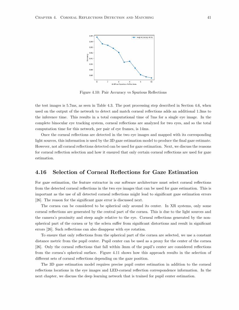
However, if we consider the effect of adding spurious reflections on the corneal reflection pairs other

than the one closest to the pupil center, then the decrease in accuracy is only 7% as seen in Figure 4.10.

4.15 Real Time Performance of the Network

We evaluate the network’s real time performance by measuring the inference time for a single eye frame

on an RTX2060 GPU. A forward pass of a 32-bit floating-point image of size 320x240 averaged across


Figure 4.10: Pair Accuracy vs Spurious Reflections

the test images is 5.7ms, as seen in Table 4.3. The post processing step described in Section 4.6, when

used on the output of the network to detect and match corneal reflections adds an additional 1.3ms to

the inference time. This results in a total computational time of 7ms for a single eye image. In the

complete binocular eye tracking system, corneal reflections are analyzed for two eyes, and so the total

computation time for this network, per pair of eye frames, is 14ms.

Once the corneal reflections are detected in the two eye images and mapped with its corresponding

light sources, this information is used by the 3D gaze estimation model to produce the final gaze estimate.

However, not all corneal reflections detected can be used for gaze estimation. Next, we discuss the reasons

for corneal reflection selection and how it ensured that only certain corneal reflections are used for gaze

estimation.

4.16 Selection of Corneal Reflections for Gaze Estimation

For gaze estimation, the feature extractor in our software architecture must select corneal reflections

from the detected corneal reflections in the two eye images that can be used for gaze estimation. This is

important as the use of all detected corneal reflections might lead to significant gaze estimation errors

[26]. The reason for the significant gaze error is discussed next.

The cornea can be considered to be spherical only around its center. In XR systems, only some

corneal reflections are generated by the central part of the cornea. This is due to the light sources and

the camera’s proximity and steep angle relative to the eye. Corneal reflections generated by the non-

spherical part of the cornea or by the sclera suffer from significant distortions and result in significant

errors [26]. Such reflections can also disappear with eye rotation.

To ensure that only reflections from the spherical part of the cornea are selected, we use a constant

distance metric from the pupil center. Pupil center can be used as a proxy for the center of the cornea

[26]. Only the corneal reflections that fall within 3mm of the pupil’s center are considered reflections

from the cornea’s spherical surface. Figure 4.11 shows how this approach results in the selection of

different sets of corneal reflections depending on the gaze position.

The 3D gaze estimation model requires precise pupil center estimation in addition to the corneal

reflections locations in the eye images and LED-corneal reflection correspondence information. In the

next chapter, we discuss the deep learning network that is trained for pupil center estimation.


(a) Two corneal reflections are selected (b) All five corneal reflections are selected

(c) Three corneal reflections are selected (d) Four corneal reflections are selected

Figure 4.11: Selection of different corneal reflections based on the gaze position. The reflections markedwith red, orange, pink, green and blue represent the different corneal reflections in the image. Only thereflections falling inside the boundary region (denoted by white) are considered for gaze estimation.

Chapter 5

Pupil Center Estimation

Our eye tracking system, along with locations of two or more corneal reflection also requires accurate

estimates of pupil center to produce a gaze estimate [26]. In the previous chapter, we already discussed

how corneal reflections could be accurately detected and matched with its originating light source within

the same neural network.

We design a UNET [29] style network for pupil center estimation. Using such an architecture allows

estimating pupil center only on a ’valid’ set of eye images. An eye image is said to be ’valid’ if at

least 50% of the pupil is visible. Estimating pupil center with high precision on occluded eye images is

challenging and usually results in significant gaze errors.

The proposed pupil estimation network’s goal is to find the region of a pupil in the eye image. The

input to the network is an image of the eye of size 320x240, while the output is a probability for each

pixel in the original image. Here the probability represents whether a pixel is part of a pupil region.

To train such a network, labels of the same size as that of input are generated, similar to the corneal

reflection network discussed in the previous chapter. Each pixel in the label image has an encoding of 1

or 0 depending on whether it belongs to a pupil. A discussion of the data collection procedure is done

next.

5.1 Data Collection

Eye images for training and testing the neural networks are recorded following the procedure similar

to the one described in the previous chapter. However, to increase pupil variability in eye images,

illumination levels of the 3D scene are varied while collecting the eye images.

Figure 5.1 illustrates the three different illumination levels of the 3D scene that have a significant

effect on the pupil’s size. Recall, that the position and orientation of light source in the 3D scene affects

the illumination levels of a scene.

Once data is collected, it must be labelled appropriately. Data labelling process is discussed next.

5.2 Data Labelling

A single person manually labelled the dataset. In the first stage of labelling, each eye region is labelled

as either a valid eye or an invalid eye. An eye region is considered invalid if the pupil is significantly

43

Chapter 5. Pupil Center Estimation 44

(a) Bright Screen (b) Small Pupil

(c) Medium Lighting (d) Medium Sized Pupil

(e) Dark Environment (f) Dilated Pupil

Figure 5.1: Effect of changing illumination in the 3D scene on the pupil size

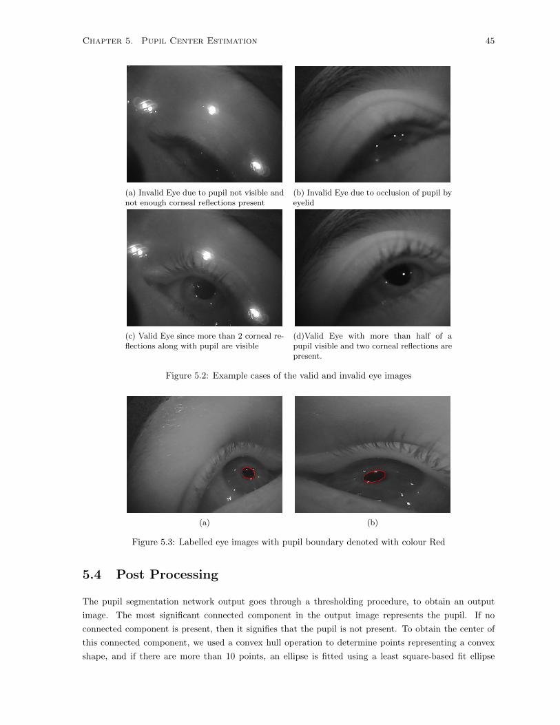
occluded, or if more than three corneal reflections are missing. Invalid eye regions can naturally occur

during a blink or rotation of the eye. Examples of eye regions labelled as valid and invalid are shown in

Figure 5.2.

In the second stage of labelling, the pupil center labels must be determined. The human annotator

first clicks on atleast 10 points along with the pupil–iris boundary on the valid eye images. These ten

boundary points are used to fit an ellipse to the pupil–iris boundary using the OpenCV function fitellipse

[91]. Labelled eye images with pupil boundary can be seen in Figure 5.3 All the pixels inside the fitted

ellipse are encoded as 1’s while all the other pixels are set as 0. This encoding of 1’s and 0’s results in a

’binary’ mask.

In the next section, we discuss the objective function used to train this network.

5.3 Objective Function

We use the same objective function as used in Corneal reflection detection and matching network (CE

+ Soft Dice) for locating pupil region in eye images. However, an additional factor is added into the

CE loss function to consider the vertical bias in pupil center estimation. Recall that this bias is due

to eyelid occlusion that occurs when the subject is gazing at lower points on the screen or during

blinking. When the eye is occluded, some of the pupil boundary pixels are not visible. This results in

the network predicting a lower probability for the pixels that belong to the pupil in the occluded region.

To ensure that the occluded pupil’s boundary pixels are estimated with higher confidence, a weighted

factor is added to the CE loss for only the pixels belonging to the pupil boundary [92]. The next section

describes the post-processing step needed to obtain the final answer from the inference network.


(a) Invalid Eye due to pupil not visible andnot enough corneal reflections present

(b) Invalid Eye due to occlusion of pupil byeyelid

(c) Valid Eye since more than 2 corneal re-flections along with pupil are visible

(d)Valid Eye with more than half of apupil visible and two corneal reflections arepresent.

Figure 5.2: Example cases of the valid and invalid eye images

(a) (b)

Figure 5.3: Labelled eye images with pupil boundary denoted with colour Red

5.4 Post Processing

The pupil segmentation network output goes through a thresholding procedure, to obtain an output

image. The most significant connected component in the output image represents the pupil. If no

connected component is present, then it signifies that the pupil is not present. To obtain the center of

this connected component, we used a convex hull operation to determine points representing a convex

shape, and if there are more than 10 points, an ellipse is fitted using a least square-based fit ellipse


function (from the OpenCV library [91]). If less than 10 points are present, then the image is deemed

an ’invalid’ eye image.

Eyelid occlusion due to the subject blinking will also affect the estimation of the pupil center. To

identify a blink, we first compute the average probability for all the pixels inside the fitted ellipse. The

average probability of pixels inside the ellipse must be above a threshold. Also, if the area of the ellipse

is above another threshold, only then an eye image is deemed to be ’valid’.

Figure 5.4, illustrates the output of the network and the resulting pupil region in the original image

as a result of applying the post processing step described above.

(a) Raw output from the network (b) Pupil After Ellipse Fitting

Figure 5.4: Post processing

In the next section, we will discuss the estimation network’s training procedure along with the related

hyperparameters search.

5.5 Hyperparameter Tuning Results

We use the same set of hyperparameters (as mentioned for the corneal reflection network in the previous

chapter) to tune the pupil center estimation network. In tuning a network’s performance, we are con-

cerned with inference quality and the time required to compute the inference. Remember that our goal

is to achieve a gaze estimation rate of at least 30 frames/s cumulatively across the two feature estimation

networks and for both eyes running on a GPU available in VR enabled laptops (RTX 2060).

The hyperparameters in Table 4.2 (can be seen in Chapter 4) were explored by training each archi-

tecture with the training dataset discussed above and measuring the quality of results on the validation

set. Training occurred for 120 epochs, with a batch size of 8 and a learning rate of 0.001. The networks

explored included Batch Normalization after every CNN layer [56] and used a ReLU activation function

[50]. The network was saved if the difference between validation and training loss showed no variation

for five consecutive epochs to permit early stopping. In training, we found that the Stochastic Gradi-

ent Descent (SGD) with momentum [58] optimizer achieved a better generalization on the test dataset

compared to self-adaptive optimizers [88].

The pupil center estimation network is evaluated on two accuracy metrics. The first accuracy metric

looks at the mean Euclidean distance error between the annotated pupil center pi and the predicted

center qi where i is one of the 4000 validation images.

Euclidean distance is given by:


EuclideanDistance =

√√√√ N∑i=1

(pi − qi)2 (5.1)

The second accuracy metric looks at the standard deviation of the Euclidean distance error in pupil

center estimation. A higher standard deviation indicates larger spread around the mean which makes a

network less reliable.

Another metric that the network was evaluated on is the computational cost of one forward inference

through the network. Precisely, this was measured as the inference time (in milliseconds), when running

on an RTX 2060 GPU. This value was determined by the neural network training’s profiler that we used

Tensorflow version 1.14 [89].

Appendix A presents the results for all the explored networks. Table 5.1 shows the results for the

networks that make use of Convolution layer with a stride of 2 as the downsampling layer in the four

downsampling blocks and Transposed convolution as the upsampling layer in the four upsampling blocks.

These networks exhibit higher accuracy than the rest of the explored networks.

There is a potential reason why the networks which make use of a Transposed CNN layer as the

upsampling layer exhbit lower error than the networks which use Bilinear Interpolation as the upsampling

layer. Due to a significant gradient change at the pupil’s boundary, Bilinear interpolation estimates pixel

values for the boundary positions with a lower probability. Recall, Bilinear interpolation [86] considers

pixels in a small neighbourhood around the upsampled position to estimate the pixel’s value. On the

contrary, Transposed CNN [54] learns the pixel values in the upsampled position using a backpropagation

algorithm. Pixels with lower probability will result in their removal from the final output according to

the post-processing steps described previously. The removal of boundary pixels has a significant effect

on the precision in the estimation of the center.

From the list of possible networks presented in Table 5.1, the network that uses Depth-Wise Convolu-

tion with a stride of 2 in each of the CNN layers in the downsampling blocks and Standard Convolution

in each of the CNN layers in the upsampling blocks exhibits the lowest mean and standard deviation of

Euclidean distance error in pupil center estimation.

ConvolutionType

inUpsampling

Blocks

ConvolutionType

inDownsampling

Blocks

Mean EuclideanDistance(pixels)

StandardDeviation

ofEuclideanDistance(pixels)

InferenceTime(ms)

Dilated Dilated 1.2 1.4 6Standard Standard 1.2 0.95 3.6

Dilated Standard 1.3 1.3 5.2Standard Dilation 1.4 1.5 4.7

Depth-Wise Standard 1.2 1 4.3Depth-Wise Depth-Wise 1.2 1.1 4.7Standard Depth-Wise 1.1 0.9 3.7

Table 5.1: Hyperparameter tuning results for the networks which uses Strided Convolution in each ofthe four downsampling blocks and Transposed CNN in each of the four upsampling blocks

To conclude the following hyperparameters are used by the selected network:


• A Depth-Wise Convolution is used in CNN layers of four downsampling blocks

• A Standard Convolution is used in the CNN layers of four upsampling blocks.

• A transposed CNN layer is used as the upsampling layer.

• For downsampling, the CNN layers in the downsampling block have a stride of 2.

Before discussing the performance of the final selected network on the test data set, it is required to

determine the threshold levels for locating the pupil region in the output probability map. This is an

important step in the post processing stage as described in Section 5.4.

The threshold level is determined from the ROC curve as seen in Figure 5.5, such that the false-

positive rate is less than 0.2. The final threshold level was determined to be a probability of 0.8. A

probability level of 0.8 corresponds to a gray-scale value of 200.

Figure 5.5: ROC for Pupil Network

In the next section, we discuss the performance of the selected network on the test dataset.

5.6 Pupil Center Estimation Performance on Test Dataset

Table 5.2 presents the pupil center estimation results on the test dataset for the selected network. The

network exhibits 1.2-pixel Euclidean distance error in pupil center estimation. The standard deviation

of the Euclidean distance error in pupil center estimation is observed to be 1.1, as illustrated in Table

5.2. The proposed network can also correctly differentiate between valid and invalid eye images, 95%

of the time. The network’s confidence level is evaluated using the Dice coefficient [90]. It measures the

similarity between the label and the output. Perfect agreement between the generated output and the

prediction gives a coefficient of 1. An average Dice coefficient of 0.94 indicates a large overlap between

the output of the network and label (a binary mask of the pupil region).

In the next section, we compare the network’s performance with state-of-the-art rule-based and deep

learning-based approaches.


ClassifierPerformance

(Valid/Invalid Eye)(%)

Mean EuclideanDistance Error

(pixels)

Standard Deviationof

Euclidean DistanceError (pixels)

Mean DiceCoefficient

MeanInference

Time (ms)

95 1.2 1.1 0.94 3.6

Table 5.2: Pupil Center Estimation Network Performance on the Test dataset

5.7 Performance Comparison with State-of-the-art Methods

Recent rule-based and deep learning approaches are optimized for pupil detection instead of pupil center

estimation. A pupil is said to be detected if the difference between labelled and the predicted center

is within 5 pixels (discussed in Chapter 2). However, for our eye tracking system, precise pupil center

estimation is a fundamental requirement. We consider two evaluating system performance methods: 1)

the precision of estimating a pupil center on our test dataset and 2) Accuracy of detecting a pupil on

publicly available datasets. In the next section, we use pupil center estimation to compare our proposed

network with the state-of-the-art methods.

Pupil Center Estimation Performance

Rule-based approaches which include PuReST, PuRe and ExCuse [68, 69, 65] (discussed in Chapter 2)

are applied to our test dataset. The pupil center obtained from the ‘valid’ eye images were analyzed.

PuReST [68] shows the lowest Euclidean distance error among all the rule-based approaches (as seen in

Table 5.3). However, the error reported by PuReST is three times more than our method. The standard

deviation of the Euclidean distance for our method is eight times less than PuReST, 11 times less than

ExCuSe, and 15 times less than PuRe. Recall that higher standard deviation indicates a larger spread

of the error around the mean, which reduces the reliability of a method.

Pupil Method/Metric PuRe PuReST ExCuse Our MethodMean Euclidean Distance

(pixels)3 3.8 5 1.2

Standard Deviationof Euclidean Distance

(pixels)15 8.5 11.2 1.1

Table 5.3: Comparison with Rule based algorithms on the test dataset

In the next section, we evaluate our network’s pupil detection performance on publicly available

datasets and compare it with state-of-the-art methods.

Pupil Detection Performance on Publicly Available Datasets

We compare our network’s pupil detection performance with both rule-based and deep learning-based

methods on the publicly available datasets LPW and Swirski [67, 66]. Both these datasets are recorded

using an off-axis camera inside a non-XR head-mounted system. Figure 5.6 shows the example images

from the two pupil detection datasets [67, 66] used in this experiment.


(a) Swirksi (b) LPW

Figure 5.6: Eye images from the two publicly available datasets

Table 5.4 presents the results for pupil detection of our network along with state-of-the-art rule

based PuRe [68], PuReST [69], ExCuSe [65]) and the deep learning-based approaches (DeepEye) [71]

and Domain-Specific Data Augmentation CNN network (DSDA) [70].

Pupil Method/Dataset PuRe PuReST ExCuse DeepEye DSDA Our MethodLPW 75 82 60 50 84 76

Swirksi 80 84 65 54 74 82

Table 5.4: Pupil Detection Rate (%) on LPW and Swriski Datasets

Our proposed network’s performance is comparable to the most accurate rule-based (PuReST) [69]

and deep learning-based (DSDA) pupil detection approach [70]. In the next section, we discuss the

real-time performance of the pupil center estimation network.

5.8 Real Time Performance of the Network

The pupil center estimation network takes around 3.6ms for completing inference on a single image of

size 320x240 with 32-bit floating-point precision on an RTX 2060 GPU. Once inference is complete, the

post processing step (as described in Section 5.4) takes around one millisecond for each eye. This means

that the total time taken by the network to produce a final answer is 4.6 ms. Since our eye tracking

system computes gaze for both left and right eye, this means that the pupil center estimation network

also has to run for the two eyes. This means that a total time of 9.2 ms for our network to produce a

final pupil center estimate for the two eyes.

5.9 Effect of Boundary Aware Loss Function

The objective function used to train the pupil center estimation network, as discussed in Section 5.3,

has a weighting factor added to the CE loss for the pixels belonging to the boundary of a pupil. The

addition of a weighting factor makes the CE loss aware of the boundary pixels.

In occluded images, to get a precise pupil center estimate, pixels that belong to the pupil’s occluded

region (these pixels are not visible) need a high probability of belonging to a pupil region in the output


probability map. Some of the occluded images can be seen in Figure 5.7. A probability lower than the

threshold used in the post-processing step will ensure that the pixels which are not visible but belong

to the pupil are removed from the final output. The removal of boundary pixels affects the precision in

the pupil center’s estimation.

The addition of this weighting factor in the CE loss helps the network estimate the boundary pixels

with a confidence higher than the threshold used in the post-processing step. We saw a 10% reduction

in the Euclidean distance error (pixels) of pupil center estimation in occluded eye images (a change from

2.3 pixel error to 2.1 pixel error) using the boundary-aware cross-entropy loss in the objective function.

The value of the weighted factor was set to 30, as used in [92].

(a) Pupil occluded by upper eyelid (b) Pupil occluded by lower eyelid

Figure 5.7: Occluded valid eye images labelled with pupil boundary

5.10 Gaze Estimation Rate

The two feature extraction networks (corneal reflection and pupil center) discussed in this and the

previous chapter cumulatively take around 24ms for finding the pupil and corneal reflections for the two

eyes on an RTX2060 GPU. The resolution of the input eye images is 320x240, with 32-bit floating-point

precision.

In our eye tracking system, once the features have been detected, it only takes a fraction of a

millisecond to compute the gaze. Hence all the time needed to produce a point-of-gaze can be attributed

to the time taken by the feature extractor, resulting in a final gaze estimation rate of 40 frames/sec.

The next chapter evaluates the end-end eye tracking system, using the designed feature extraction

networks, the calibrator, and the 3D gaze estimation model.

Chapter 6

Eye Tracking Results

This chapter describes a series of experiments to determine the performance of the end-end eye tracking

system (see Chapter 3) using the feature extraction methods outlined in Chapters 4 and 5. The results of

these experiments are compared to the results of state-of-the-art XR and non-XR eye tracking systems.

Eye tracking performance is usually measured by computing the error between the actual and the

predicted point-of-gaze. The actual points are specific targets placed on a display screen (in case of XR

systems) or in the real world (in case of non-XR systems). The predicted points are the gaze estimates

produced by an eye tracking system. Head-mounted system performance can be evaluated either when

the eye tracking system is fixed relative to the head or when the eye tracking system moves relative to the

head. The eye tracker’s movement is also referred to as headset slippage. Recall that the fundamental

requirements of a head-mounted eye tracking system require high accuracy and insensitivity to headset

slippage.

The analysis for all the experiments in this chapter was done offline, which means that the eye images

could be captured at a higher frame rate of 90 frames/sec than the online gaze estimation rate of the

eye tracking system (as discussed in the previous chapter).

6.1 Eye Tracking Performance with no Headset slippage

The system’s performance was evaluated with six subjects. Each subject first completed a calibration

procedure. During the procedure, subjects fixated on the center of a circular target. The target point

moves every two seconds to a new location within a box of ± 5◦ (total of 9 locations). The fixation

distance in the 3D scene for all target locations was set to 1m. The range of the calibration target on the

display screen was kept relatively small to maximize the probability of computing calibration parameters

for all of the ten corneal reflections pairs (see Chapter 3). The calibration procedure computes the

subject-specific eye parameters for all the pairs of corneal reflections.

Following the calibration procedure, subjects were asked to remove the headset and wear the headset

again to test the system. This was done to demonstrate that an eye tracking system that uses the

3D gaze estimation model does not require repeated calibration procedures [26]. This is in contrast

to some current XR and non-XR eye tracking systems that use feature-based gaze estimation methods

and require recalibration every time a user wears the headset [39]. While our system does not require

recalibration, we perform a short bias correcting step every time a user wears the headset to align the

52

Chapter 6. Eye Tracking Results 53

display and eye coordinate systems [26]. In the bias correcting step, subjects look at the center of the

display for 2 seconds, and the horizontal and vertical deviations (biases) from the center of the display

are measured. We add these biases to the gaze estimates produced by our system.

With known calibration parameters and system information, the 3D gaze estimation model [26]

computes the point-of-gaze. To test the eye tracker’s performance, targets were moved in the horizontal

and vertical direction to nine different positions within a box spanning a range of ± 10◦. At each target

position, the target was stationary for two seconds. Gaze estimates corresponding to eye movements in

response to the change in target positions were ignored (data collection for each target position started

after a delay of 300ms from the time that the target position was changed). Fixation distances in the

3D scene were either 1m or 2m.

In the next section, we discuss the parameters used for the evaluation of our eye tracking system.

6.1.1 Performance Metrics

We evaluate system performance using the following three metrics [33]. These include:

• Accuracy: The Euclidean distance between the estimated point-of-gaze and the target location.

• Precision: The root mean square difference between two consecutive estimates of the points-of-gaze

during fixations on the same target.

• Data Loss: The number of missing samples expressed as a percentage of the expected number of

samples for each target.

In the next section, we evaluate our eye tracking system using the above three performance metrics.

6.1.2 Eye tracking Performance

Figure 6.1 shows the raw gaze estimates for one of the six subjects at a fixation distance of 1m while

the user was gazing at the nine target positions. At each target position, our system computes gaze

estimates for 2 seconds. At 90 frames/sec, this corresponds to 180 gaze estimates.

Figure 6.2 shows heat-maps for the three performance metrics at the nine target positions. For each

target position, the performance metrics were computed by averaging gaze estimates of all six subjects

at fixation distances of 1m and 2m. Three statistical measures describe the accuracy at the nine target

position: mean accuracy, median accuracy and standard deviation of the accuracy.

Our eye tracking system shows a median accuracy of 1◦ and a mean accuracy of 1.1 ◦averaged across

the nine target points. The standard deviation of the accuracy is consistent across all the nine target

points with an average value of 0.78◦(can be seen in Figure 6.2 (c)). A higher standard deviation of

0.78◦attributes to the variable number of corneal reflections used for gaze estimation.

The system’s accuracy at the center of the display is better than the accuracy at the four corners of

the display (Figure 6.2 (a), (b)). This is mainly due to the reduced number of corneal reflection pairs in

eye images at the four corners.

Figure 6.2 (d) shows that our system exhibits consistent high precision at all the nine target points

for the six subjects. High precision with negligible data loss Figure 6.2 (e) across the target points

reflects the robustness of the deep learning-based feature extractor to changes in the appearance of eye

features in eye images.


Figure 6.1: Raw gaze estimates at ± 10◦for the nine target position at 1m fixation distance

6.2 Comparison with State-of-the-art Eye Tracking Systems

We compare our system performance with that of state-of-the-art XR and non-XR head-mounted sys-

tems. State-of-the-art non-XR eye tracking systems include Tobii [93], Pupil Labs [38] and SMI [94].

These systems are commercially available eye trackers evaluated in [33]. State-of-the-art XR systems

include machine learning-based systems including NvGaze [1] and EyeNet [32].

Table 6.1 presents the comparison results of our system with the non-XR systems. Please note that

for non-XR systems, median accuracy across the nine points is reported in [33]. Our system has a 40%

higher median accuracy averaged across the nine target points compared to the best performing non-XR

head-mounted eye tracking system (SMI). While data loss and precision across the nine target points

of our system are comparable with SMI [94], the average standard deviation of the accuracy across the

nine points is slightly higher. The reason for the higher standard deviation has already been discussed

in Section 6.1.

Pupil Labs [38], which uses a feature-based method to compute the final point-of-gaze, exhibits lower

accuracy than our system. Later in this chapter, we will show that both Pupil Labs and SMI are sensitive

to headset slippage.

Eye Tracker/Metric Tobii Pupil Labs Grip SMI Our SystemAccuracy (◦) 2.6 2.3 1.6 1.4 1Precision (◦) 0.3 0.1 0.85 0.11 0.13

Standard Deviation (◦) 0.6 0.22 0.77 0.3 0.78Data Loss (%) 4 0.5 1.54 0 0

Table 6.1: Comparison with non-XR systems

Table 6.2 presents the results for eye tracking systems that were designed for XR applications. For

these systems, only mean accuracy is reported across the test points. Our system’s mean accuracy across

the target points is 100% more than NvGaze [1] and 200% more than EyeNet [32].


(a) Median Accuracy (b) Mean Accuracy

(c) Standard Deviation of Accuracy (d) Precision

(e) Data Loss

Figure 6.2: Performance metrics for target points placed at ±10 ◦

Eye Tracker/Metric NvGaze EyeNet Our SystemAccuracy (◦) 2.1 3 1.1

Table 6.2: Comparison with learning based XR systems (◦)

State-of-the-art XR eye tracking systems do not provide any information regarding the target loca-

tions during testing. As gaze estimation errors increase for peripheral targets [39], we further analyze

our system’s performance at a much broader FOV of ±15◦.


Figure 6.3: Raw gaze estimates at ± 15◦for every target position

6.3 Testing the System at a Larger Field of View

Figure 6.3 shows the raw gaze estimates for one of the six subjects at a fixation distance of 1m while

the user is gazing at nine target positions at ± 15◦on the screen. At each target position and for every

fixation distance, our system computes 180 gaze estimates.

Figure 6.4 shows the heat-maps for the three performance metrics at the nine test points for all six

subjects. Three statistical measures describe the accuracy at the nine target position: mean accuracy,

median accuracy and standard deviation of the accuracy.

Our system exhibits worse performance for the peripheral target points relative to the results obtained

at 10◦ (discussed in Section 6.1). Poor accuracy at the periphery attributes to lens distortion [39].

In this section, we discussed our eye tracking system’s performance when the eye tracker is stable

relative to the head. However, since most applications for XR systems require head movements, eye

tracker, which is attached to the XR headset keeps changing its position relative to the head. This

movement is also known as headset slippage. In the next section, we discuss the performance of our eye

tracking system under headset slippage.

6.4 Eye Tracking Performance with Headset Slippage

We use the same procedure that was outlined in [33] to evaluate our eye tracking system’s performance

when the headset moves relative to the eyes (headset slippage). Each of the six subjects moved the

VR headset up/down and left/right at approximately 1Hz, where each motion lasted 10 seconds (10

cycles). During the headset movements, subjects fixated on a stationary target (stationary relative to

the subject’s eyes), and therefore, changes in eye-position during the test indicate noise induced by

movements of the headset.

To ensure that the target is stationary relative to the eyes, we defined the target’s coordinates on

the VR display in the 3D world coordinate system. Please note that the eye tracker’s gaze estimates


(a) Median Accuracy (b) Mean Accuracy

(c) Standard Deviation of Accuracy (d) Precision

(e) Data Loss

Figure 6.4: Performance metrics at ± 15◦

are computed in the coordinate system of a virtual camera attached to the headset and not in the 3D

world coordinate system (described in Chapter 3). This means that if the headset moves, the target

on display will move in the opposite direction so that the target will appear stationary to the subject

in the 3D world coordinate system. As the eye tracker’s gaze estimates are relative to the display, the

subject eye movements will be in a direction opposite to that of the headset. Headset tracking sensors

track the headset in the real world, and the headset’s position is used by the Unity 3D game engine [36]

(a detailed description of the software system is provided in Chapter 3) to update the position of the

target during headset movements.

The experiment described in [33] for eye tracker evaluation with headset slippage is divided into two

stages. In the first stage, with no intentional headset slippage, subjects are instructed to fixate for ten

seconds on a target placed at the center of the display. The first stage results are used as a baseline for


comparison with the results of the second stage.

Figure 6.5 shows the horizontal and vertical gaze estimates and the corresponding target positions

during baseline reading for one of the subjects. In a few instances, there are transient changes of 1.5◦

in the horizontal and vertical gaze estimates. These errors attribute to blinking. The blinking of the

user results in eye images that are significantly occluded. Gaze estimates, if computed on such occluded

images, are prone to errors.

The second stage of the experiment involves subjects fixating on a stationary target in the 3D world

coordinate system, while the headset moved in the up/down direction for 10 seconds and then the

left/right direction for 10 seconds. The range of movements in each direction was 5mm. Table 6.3

presents the results of these experiments for our system and the non-XR systems, as reported in [33].

During the headset movements, there is an average change of 1.3◦ (0.6◦ to 1.9◦) in gaze estimation

accuracy relative to the baseline.

Eye Tracker/Experiment Stage Tobii Pupil Labs Grip SMI Our SystemBaseline Reading 0.8 1.8 1.1 1.0 0.6

Movement 1.5 8 1.8 18 1.9

Table 6.3: Mean Accuracy during headset slippage (◦)

These results are worse than the results obtained for non-XR systems such as Tobii [93] (0.7◦) and

Grip [42] (0.7◦). Three factors contribute to the higher sensitivity of our system to headset movements:

• Subjects have to look through the non-central part of the VR lens during headset slippage. Dis-

tortion due to the lens at these instances will lead to a distorted view of the fixation target and

add bias to the eye tracker’s gaze estimates (we observed this in the previous experiment for the

points placed within 15◦under no headset slippage).

• The second and the most important reason is the delay between the time at which the head tracker

tracks the headset position in the real world and the time at which VR display renders the target.

When the headset changes its direction in the real world, the VR head tracker sends the new

headset position information to the Unity 3D game engine, and then the target position on the

display is updated. This process takes time, and during this time, the display’s target still moves in

the direction of the headset. The result is gaze estimates that follow the target on display showing

more significant transient changes than the target locations. This can be seen in Figure 6.6 (c),

where under the up/down movement of the eye tracker, the target exhibits transient changes up

to 2◦ while the gaze following the target in the vertical direction shows changes up to 4◦. Both

the gaze and target are defined in the virtual camera coordinate system.

Figure 6.7 shows the positions of the target (on the visual display) and the computed raw gaze

estimates in the horizontal and vertical direction during the left/right (horizontal) movement of

the headset. The horizontal movement of the headset over time can be observed in Figure 6.7 (c).

The horizontal gaze estimates and the target locations defined in the virtual camera coordinate

system exhibit a transient change during the headset’s left/right movement (as seen in Figure 6.7

(b)). The transient changes in the target location (indicated by red colour) are as high as 2◦, while

a transient change in horizontal gaze estimates is as high as 4◦. No effect of left/right headset

movement can be seen on the vertical gaze estimates (Figure 6.7 (a)).


(a) Horizontal Gaze and Target locations

(b) Vertical Gaze and Target locations

(c) Headset Movement

Figure 6.5: Gaze estimates, target locations and headset position during no headset slippage

• The third factor that contributes to gaze error during headset slippage is due to changes in the

number of pairs of corneal reflections that are used for the computation of the point of gaze when

the headset moves.


(a) Vertical Headset Movement

(b) Horizontal Gaze and Target Locations in the VirtualCamera Coordinate Systems

(c) Vertical Gaze and Target Locations in the VirtualCamera Coordinate Systems

Figure 6.6: Gaze estimates, target locations and headset position during the up/down movement of theheadset

None of these issues affect the non-XR system’s performance since no physical screen or lenses are


attached to the headset. Even with the issues described above, our eye tracking system exhibits a mean

accuracy of 1.9◦ under continuous headset slippage. This is comparable to the best performing non-XR

eye tracking systems, which includes Tobii [93] and Grip [42]. On the contrary, SMI [94], which showed

the most promising results under no headset slippage (discussed in the previous section), is affected the

most by headset slippage with reported accuracy much worse than our system. Also, Pupil Labs [38],

which uses feature-based methods for gaze estimation, reports four times less accuracy relative to our

system during headset slippage.


(a) Vertical Gaze and Target Locations in the VirtualCamera Coordinate System

(b) Horizontal Gaze and Target Locations in the VirtualCamera Coordinate System

(c) Horizontal Headset Movement

Figure 6.7: Gaze estimates, target locations and headset position during the left/right movement of theheadset

Chapter 7

Conclusion and Future Work

This chapter provides a conclusion for the research work and directions that can be taken in the future.

7.1 Conclusion

We have presented an eye tracking system designed for XR applications using commercially available

eye tracking hardware module from Pupil Labs [31] and a VR headset [34]. Our system which uses the

3D gaze estimation model satisfies the four fundamental requirements for an XR eye tracking system

which includes: 1) high accuracy, 2) maintenance of high accuracy irrespective of fixation distance, 3)

robustness to headset slippage and 4) high gaze estimation rate (¿ 25 Hz). The eye tracker uses a 3D

gaze estimation model that requires a one-time calibration procedure and accurate estimation of eye

features that include pupil center and corneal reflections. The 3D Model also requires knowledge of the

correspondence between the corneal reflections and their originating light sources.

Feature estimation is relatively tricky in XR systems due to the physical constraints that result in

the camera placed at a significant off-axis angle relative to the eye’s optical axis with the LED’s having

steep illumination angles. These physical constraints result in poor-quality eye-images and inconsistent

patterns of eye-illumination. The inconsistent patterns make the determination of the correspondences

between corneal reflections and their light sources, a very challenging problem.

In this work, we present a novel deep learning-based feature extractor developed for VR devices to

estimate the position of eye-features and find the correspondence between corneal reflections and light

sources. Our deep learning-based feature extractor consists of two separate networks for the two eye

features: pupil and corneal reflections. Both the networks make use of the UNET architecture, to find

the regions in the image that belongs to the pupil and corneal reflections. The pupil center estimation

network can estimate the pupil center with an average Euclidean distance error of 1.2 pixels. The corneal

reflection detection and matching network can detect and match each of the five corneal reflections with

their light source, with an average accuracy of 91%. The feature extractor networks for the two eyes

cumulatively run at 40 frames/sec on a GPU available in standard gaming laptops, thus enabling low

latency eye tracking.

We evaluate our eye tracking system under two scenarios: 1) when the eye tracker is fixed relative

to the head and 2) when the eye tracker moves relative to the head. The eye tracker movement is also

known as headset slippage. For each scenario, the system was tested on six subjects.

63

Chapter 7. Conclusion and Future Work 64

In scenario 1, every subject was asked to look at the points placed within a box that spanned a

field of view ± 10◦. Our system reports a median accuracy of 1◦averaged across the nine target points.

This is 40% better than the best performing non-XR eye tracking system. Our system reports a mean

accuracy of 1.1◦, which is 100% better than learning-based XR eye tracking systems.

For scenario 2, the experiment was performed in two stages. In the first stage, under no headset

slippage, subjects are instructed to fixate for ten seconds on a target placed at the center of the display.

The results from the first stage are used as a baseline for comparing the results from the second stage.

In the second stage, each subject moved the VR headset up/down and left/right at a frequency of 1Hz,

where each motion lasted 10 seconds (10 cycles). During the headset movements, subjects fixated on

a stationary target (stationary relative to the subject’s eyes), and therefore, eye-movements during the

test indicate noise induced by movements of the headset.

Our system shows an average variation of 1.3◦under horizontal and vertical device movement relative

to the baseline reading. Most of this variation can be attributed issues relevant only to XR systems that

include constrained eye relief, lens distortion and a lack of synchronization between the head tracker and

the display. Even under the presence of the above-listed issues, our system reports a mean accuracy of

1.9◦, comparable with the best performing state-of-the-art non-XR eye tracking systems.

7.2 Future Work

Many avenues are available to extend and improve the capability of the novel XR eye tracking system

presented in this work.

7.2.1 Use of On-Axis Camera Configuration

Our eye tracking system has the camera placed off-axis relative to the optical axis of the eye. The result

of using an off-axis camera is eye images that are distorted and change dramatically with eye movements.

Recall that this makes accurate feature extraction, especially corneal reflection detection and matching,

much more challenging.

With the use of an on-axis camera configuration, the quality of the eye images significantly improves.

Such a camera configuration is typical in recent commercial eye trackers designed for XR systems. One

such system from Tobii [93] can be seen in Figure 7.1. Here, the light sources are placed around the

lens, but the camera finds its place between the two VR lenses. Using our eye tracking system inside

such a VR headset will further boost our system’s performance and accuracy.

7.2.2 Synchronization Between Camera and Light sources

One of the reasons why the detection of corneal reflections among spurious reflection is a challenging task

for our system is the lack of synchronization between the camera and light sources. Ideally, only when

the camera captures the image should the light sources be ON to reduce image smear. Image smearing

results in corneal reflections to appear either very dim or disappear altogether. Synchronization between

light sources and the camera will allow LED to turn ON only when the camera is capturing the eye

image.

Chapter 7. Conclusion and Future Work 65

Figure 7.1: Tobii VR

7.2.3 Reducing the Effects of Lens Distortion

We evaluate our system on points placed within the FOV of 10◦and 15◦. In our system, to robustly track

corneal reflections, the subject’s eyes were placed relatively far away from the lens of the VR system.

With such placement, significant lens distortion is experienced when gazing at points placed at 15◦.

In the future, installing the light sources in a way that is not affected by the distance between the lens

and the eye will enable testing the system at points placed in a larger field of view with a minimal effect

of lens distortion.

7.2.4 Eye tracking System for Augmented or Mixed Reality

Our eye tracking system is designed in the context of Virtual Reality. We chose to select Virtual Reality

as it is among the most popular XR system in the consumer market today. However, other XR devices

that include Augmented and Mixed Reality are also seeing a rise in consumer adoption. Companies such

as Microsoft [95] and Magic Leap [96] are launching standalone mixed reality headsets.

An IR camera (placed on-axis or off-axis) and multiple IR light sources installed on such devices can

use the eye tracking system proposed in this work for a VR headset for an AR or MR headset. The

only significant modification required when making use of the proposed system is the retraining of the

corneal reflection detection and matching network. Recall that this network is dependent on the number

of light sources used to illuminate the eye region.

Appendix A

Hyperparameter Tuning Results

A.1 Hyperparameter Results for the Pupil Center Estimation

Network

ConvolutionType

inUpsampling

Blocks

ConvolutionType

inDownsampling

Blocks

MeanEuclideanDistance(pixels)


Euclidean Distance(pixels)

InferenceTime(ms)

Standard Standard 1.2 1 3.6Depth-Wise Standard 1.2 1 4.5Depth-Wise Depth-Wise 1.2 1.2 4.9

Standard Depth-Wise 1.1 1 4

Table A.1: Hyperparameter results for pupil center networks when used Strided Convolution in the fourdownsampling blocks and Bilinear Interpolation in the four upsampling blocks

ConvolutionType

inUpsampling

Blocks

ConvolutionType

inDownsampling

Blocks




InferenceTime(ms)

Standard Standard 1.5 1.3 3.2Depth-Wise Standard 1.2 1.2 4.1Depth-Wise Depth-Wise 1.3 1.4 4.3

Standard Depth-Wise 1.3 1.5 3.5

Table A.2: Hyperparameter results for pupil center networks when used Strided Convolution in each ofthree downsampling blocks and Bilinear Interpolation in each of the three upsampling blocks

66

Appendix A. Hyperparameter Tuning Results 67

ConvolutionType

inUpsampling

Blocks

ConvolutionType

inDownsampling

Blocks




InferenceTime(ms)

Dilated Dilated 1.3 1.5 5.8Standard Standard 1.2 1 3.4

Dilation Standard 1.3 1.4 5Standard Dilated 1.4 1.5 4.5

Depth-Wise Standard 1.1 1 4.1Depth-Wise Depth-Wise 1.1 1 4.6

Standard Depth-Wise 1.1 1 3.5

Table A.3: Hyperparameter results for pupil center networks when used Max Pooling in each of the fourdownsampling blocks and Transposed CNN in each of the four upsampling blocks.

ConvolutionType

inUpsampling

Blocks

ConvolutionType

inDownsampling

Blocks




InferenceTime(ms)

Dilated Dilated 1.3 1.7 5.4Standard Standard 1.3 1.2 3.1

Dilation Standard 1.6 1.5 4.7Standard Dilated 1.5 1.6 4.2

Depth-Wise Standard 1.3 1.3 3.4Depth-Wise Depth-Wise 1.3 1.3 4.2

Standard Depth-Wise 1.4 1.2 3.2

Table A.4: Hyperparameter results for pupil center networks when using Max Pooling in each of thethree downsampling blocks and Transposed CNN in each of the three upsampling blocks

A.2 Hyperparameter Results for the Corneal Reflection Detec-

tion and Matching Network


Convolutionin

Upsampling

Convolutionin

Downsampling


InferenceTime(ms)

DilatedCNN

DilatedCNN

91 6

StandardCNN

StandardCNN

87 3.7

DilationStandard

CNN92 5.2

StandardCNN

DilatedCNN

88 4.7

Depth-WiseCNN

StandardCNN

89 4.2

Depth-WiseCNN

Depth-WiseCNN

86 4.0

StandardCNN

Depth-WiseCNN

88 4.2

Table A.5: Hyperparameter results for corneal reflections networks when max pooling used as downsam-pling with Bilinear Interpolation as upsampling layer. Number of blocks set to 3

Convolutionin

Upsampling

Convolutionin

Downsampling


InferenceTime(ms)

DilatedCNN

DilatedCNN

86 5.5

StandardCNN

StandardCNN

85 3.4

DilatedCNN

StandardCNN

88 4.9

StandardCNN

DilatedCNN

84 4.2

Depth-WiseCNN

StandardCNN

78 3.8

Depth-WiseCNN

Depth-WiseCNN

80 4.0

StandardCNN

Depth-WiseCNN

81 3.7

Table A.6: Hyperparameter results for corneal reflections networks when max pooling used as downsam-pling with Transposed CNN as upsampling layer. Number of blocks set to 4


Convolutionin

Upsampling

Convolutionin

Downsampling


InferenceTime(ms)

Depth-WiseCNN

StandardCNN

80 3.8

Depth-WiseCNN

Depth-WiseCNN

82 4.0

StandardCNN

Depth-WiseCNN

83 3.7

StandardCNN

StandardCNN

82 3.4

Table A.7: Hyperparameter results for corneal reflections networks when strided CNN used as down-sampling with Transposed CNN as upsampling layer. Number of blocks set to 4

Convolutionin

Upsampling

Convolutionin

Downsampling


InferenceTime(ms)

Depth-WiseCNN

StandardCNN

75 3.5

Depth-WiseCNN

Depth-WiseCNN

77 3.7

StandardCNN

Depth-WiseCNN

81 3.4

StandardCNN

StandardCNN

81 3.2

Table A.8: Hyperparameter results for corneal reflections networks when strided CNN used as down-sampling with Transposed CNN as upsampling layer. Number of blocks set to 3

Bibliography

[1] J. Kim, M. Stengel, A. Majercik, S. De Mello, D. Dunn, S. Laine, M. McGuire, and D. Luebke,

“Nvgaze: An anatomically-informed dataset for low-latency, near-eye gaze estimation,” in Proceed-

ings of the 2019 CHI Conference on Human Factors in Computing Systems, 2019, pp. 1–12.

[2] M. Eizenman, H. Y. Lawrence, L. Grupp, E. Eizenman, M. Ellenbogen, M. Gemar, and R. D.

Levitan, “A naturalistic visual scanning approach to assess selective attention in major depressive

disorder,” Psychiatry research, vol. 118, no. 2, pp. 117–128, 2003.

[3] J. Chung, “A novel test of implicit memory; an eye tracking study,” International Journal of Applied

Mathematics, Electronics and Computers, vol. 2, no. 4, pp. 45–48, 2014.

[4] T. Falck-Ytter, S. Bolte, and G. Gredeback, “Eye tracking in early autism research,” Journal of

neurodevelopmental disorders, vol. 5, no. 1, p. 28, 2013.

[5] H. Istance, S. Vickers, and A. Hyrskykari, “Gaze-based interaction with massively multiplayer on-

line games,” in CHI’09 Extended Abstracts on Human Factors in Computing Systems, 2009, pp.

4381–4386.

[6] P. Isokoski, M. Joos, O. Spakov, and B. Martin, “Gaze controlled games,” Universal Access in the

Information Society, vol. 8, no. 4, p. 323, 2009.

[7] V. Sundstedt, “Gazing at games: using eye tracking to control virtual characters,” in ACM SIG-

GRAPH 2010 Courses, 2010, pp. 1–160.

[8] M. Wedel and R. Pieters, “A review of eye-tracking research in marketing,” in Review of marketing

research. Routledge, 2017, pp. 123–147.

[9] T. Hayami, K. Matsunaga, K. Shidoji, and Y. Matsuki, “Detecting drowsiness while driving by

measuring eye movement-a pilot study,” in Proceedings. The IEEE 5th International Conference on

Intelligent Transportation Systems. IEEE, 2002, pp. 156–161.

[10] T. E. Hutchinson, K. P. White, W. N. Martin, K. C. Reichert, and L. A. Frey, “Human-computer

interaction using eye-gaze input,” IEEE Transactions on systems, man, and cybernetics, vol. 19,

no. 6, pp. 1527–1534, 1989.

[11] K.-N. Kim and R. Ramakrishna, “Vision-based eye-gaze tracking for human computer interface,”

in IEEE SMC’99 Conference Proceedings. 1999 IEEE International Conference on Systems, Man,

and Cybernetics (Cat. No. 99CH37028), vol. 2. IEEE, 1999, pp. 324–329.

70

Bibliography 71

[12] L. E. Sibert and R. J. Jacob, “Evaluation of eye gaze interaction,” in Proceedings of the SIGCHI

conference on Human Factors in Computing Systems, 2000, pp. 281–288.

[13] M. N. J. Dani, “Impact of virtual reality on gaming,” Virtual Reality, vol. 6, no. 12, 2019.

[14] M. Hsieh and J. Lee, “Preliminary study of vr and ar applications in medical and healthcare

education,” J Nurs Health Stud, vol. 3, no. 1, p. 1, 2018.

[15] K. Srivastava, R. Das, and S. Chaudhury, “Virtual reality applications in mental health: Challenges

and perspectives,” Industrial psychiatry journal, vol. 23, no. 2, p. 83, 2014.

[16] S. Barnes, “Understanding virtual reality in marketing: Nature, implications and potential,” Im-

plications and Potential (November 3, 2016), 2016.

[17] S. Gradl, B. M. Eskofier, D. Eskofier, C. Mutschler, and S. Otto, “Virtual and augmented reality

in sports: an overview and acceptance study,” in Proceedings of the 2016 ACM International Joint

Conference on Pervasive and Ubiquitous Computing: Adjunct, 2016, pp. 885–888.

[18] B. Guenter, M. Finch, S. Drucker, D. Tan, and J. Snyder, “Foveated 3d graphics,” ACM Transac-

tions on Graphics (TOG), vol. 31, no. 6, pp. 1–10, 2012.

[19] G. Kramida, “Resolving the vergence-accommodation conflict in head-mounted displays,” IEEE

transactions on visualization and computer graphics, vol. 22, no. 7, pp. 1912–1931, 2015.

[20] D. M. Hoffman, A. R. Girshick, K. Akeley, and M. S. Banks, “Vergence–accommodation conflicts

hinder visual performance and cause visual fatigue,” Journal of vision, vol. 8, no. 3, pp. 33–33,

2008.

[21] S. Reichelt, R. Haussler, G. Futterer, and N. Leister, “Depth cues in human visual perception

and their realization in 3d displays,” in Three-Dimensional Imaging, Visualization, and Display

2010 and Display Technologies and Applications for Defense, Security, and Avionics IV, vol. 7690.

International Society for Optics and Photonics, 2010, p. 76900B.

[22] L. Yang, J. HUANG, T. Feng, W. Hong-An, and D. Guo-Zhong, “Gesture interaction in virtual

reality,” Virtual Reality & Intelligent Hardware, vol. 1, no. 1, pp. 84–112, 2019.

[23] F. Hulsmann, T. Dankert, and T. Pfeiffer, “Comparing gaze-based and manual interaction in a

fast-paced gaming task in virtual reality,” in Proceedings of the Workshop Virtuelle & Erweiterte

Realitat 2011, 2011.

[24] F. L. Luro and V. Sundstedt, “A comparative study of eye tracking and hand controller for aiming

tasks in virtual reality,” in Proceedings of the 11th ACM Symposium on Eye Tracking Research &

Applications, 2019, pp. 1–9.

[25] R. Albert, A. Patney, D. Luebke, and J. Kim, “Latency requirements for foveated rendering in

virtual reality,” ACM Transactions on Applied Perception (TAP), vol. 14, no. 4, pp. 1–13, 2017.

[26] E. D. Guestrin and M. Eizenman, “General theory of remote gaze estimation using the pupil center

and corneal reflections,” IEEE Transactions on biomedical engineering, vol. 53, no. 6, pp. 1124–1133,

2006.

Bibliography 72

[27] B. Brousseau, J. Rose, and M. Eizenman, “Hybrid eye-tracking on a smartphone with cnn feature

extraction and an infrared 3d model,” Sensors, vol. 20, no. 2, p. 543, Jan 2020. [Online]. Available:

http://dx.doi.org/10.3390/s20020543

[28] B. Brousseau, J. Rose, and M. Eizenman, “Smarteye: An accurate infrared eye tracking system for

smartphones,” in 2018 9th IEEE Annual Ubiquitous Computing, Electronics Mobile Communication

Conference (UEMCON), 2018, pp. 951–959.

[29] O. Ronneberger, P. Fischer, and T. Brox, “U-net: Convolutional networks for biomedical image

segmentation,” in International Conference on Medical image computing and computer-assisted

intervention. Springer, 2015, pp. 234–241.

[30] N. Pino, “Htc vive review,” 2016.

[31] “Pupil labs vr/ar add-on,” https://pupil-labs.com/products/vr-ar/, accessed: 2020-06-21.

[32] Z. Wu, S. Rajendran, T. Van As, V. Badrinarayanan, and A. Rabinovich, “Eyenet: A multi-task

deep network for off-axis eye gaze estimation,” in 2019 IEEE/CVF International Conference on

Computer Vision Workshop (ICCVW). IEEE, 2019, pp. 3683–3687.

[33] D. C. Niehorster, T. Santini, R. S. Hessels, I. T. Hooge, E. Kasneci, and M. Nystrom, “The impact

of slippage on the data quality of head-worn eye trackers,” Behavior Research Methods, pp. 1–21,

2020.

[34] “Htc vive,” https://www.vive.com/eu/product/#vive%20series, accessed: 2020-06-21.

[35] “Opensimulator,” http://opensimulator.org/wiki/Main Page, accessed: 2020-06-21.

[36] “Unity3d,” https://unity.com/, accessed: 2020-06-21.

[37] “Unreal,” https://www.unrealengine.com/en-US/, accessed: 2020-06-21.

[38] M. Kassner, W. Patera, and A. Bulling, “Pupil: an open source platform for pervasive eye tracking

and mobile gaze-based interaction,” in Proceedings of the 2014 ACM international joint conference

on pervasive and ubiquitous computing: Adjunct publication, 2014, pp. 1151–1160.

[39] V. Clay, P. Konig, and S. Konig, “Eye tracking in virtual reality,” Journal of Eye Movement

Research, vol. 12, no. 1, Apr. 2019. [Online]. Available: https://bop.unibe.ch/JEMR/article/view/

4332-Clay-final-sub

[40] S.-H. Lee, J.-Y. Lee, and J.-S. Choi, “Design and implementation of an interactive hmd for wearable

ar system,” in 2011 17th Korea-Japan Joint Workshop on Frontiers of Computer Vision (FCV).

IEEE, 2011, pp. 1–6.

[41] M. Mansouryar, J. Steil, Y. Sugano, and A. Bulling, “3d gaze estimation from 2d pupil positions

on monocular head-mounted eye trackers,” in Proceedings of the Ninth Biennial ACM Symposium

on Eye Tracking Research & Applications, 2016, pp. 197–200.

[42] T. Santini, D. C. Niehorster, and E. Kasneci, “Get a grip: slippage-robust and glint-free gaze

estimation for real-time pervasive head-mounted eye tracking,” in Proceedings of the 11th ACM

symposium on eye tracking research & applications, 2019, pp. 1–10.

http://dx.doi.org/10.3390/s20020543

https://pupil-labs.com/products/vr-ar/

https://www.vive.com/eu/product/#vive%20series

http://opensimulator.org/wiki/Main_Page

https://unity.com/

https://www.unrealengine.com/en-US/

https://bop.unibe.ch/JEMR/article/view/4332-Clay-final-sub

https://bop.unibe.ch/JEMR/article/view/4332-Clay-final-sub

Bibliography 73

[43] P. Shi, M. Billeter, and E. Eisemann, “Salientgaze: Saliency-based gaze correction in virtual reality,”

Computers & Graphics, 2020.

[44] L. R. Young and D. Sheena, “Eye-movement measurement techniques.” American Psychologist,

vol. 30, no. 3, p. 315, 1975.

[45] A. Villanueva, R. Cabeza, and S. Porta, “Eye tracking: Pupil orientation geometrical modeling,”

Image and Vision Computing, vol. 24, no. 7, pp. 663–679, 2006.

[46] J.-G. Wang, E. Sung, and R. Venkateswarlu, “Estimating the eye gaze from one eye,” Computer

Vision and Image Understanding, vol. 98, no. 1, pp. 83–103, 2005.

[47] A. Villanueva and R. Cabeza, “Models for gaze tracking systems,” EURASIP Journal on Image

and Video Processing, vol. 2007, pp. 1–16, 2007.

[48] J. Schmidhuber, “Deep learning in neural networks: An overview,” Neural networks, vol. 61, pp.

85–117, 2015.

[49] Z.-Q. Zhao, P. Zheng, S.-t. Xu, and X. Wu, “Object detection with deep learning: A review,” IEEE

transactions on neural networks and learning systems, vol. 30, no. 11, pp. 3212–3232, 2019.

[50] A. Krizhevsky, I. Sutskever, and G. E. Hinton, “Imagenet classification with deep convolutional

neural networks,” in Advances in neural information processing systems, 2012, pp. 1097–1105.

[51] J. Gu, Z. Wang, J. Kuen, L. Ma, A. Shahroudy, B. Shuai, T. Liu, X. Wang, G. Wang, J. Cai et al.,

“Recent advances in convolutional neural networks,” Pattern Recognition, vol. 77, pp. 354–377,

2018.

[52] X. Lei, H. Pan, and X. Huang, “A dilated cnn model for image classification,” IEEE Access, vol. 7,

pp. 124 087–124 095, 2019.

[53] F. Chollet, “Xception: Deep learning with depthwise separable convolutions, 2016,” arXiv preprint

arXiv:1610.02357, 2016.

[54] V. Dumoulin and F. Visin, “A guide to convolution arithmetic for deep learning,” arXiv preprint

arXiv:1603.07285, 2016.

[55] D. Scherer, A. Muller, and S. Behnke, “Evaluation of pooling operations in convolutional architec-

tures for object recognition,” in International conference on artificial neural networks. Springer,

2010, pp. 92–101.

[56] S. Ioffe and C. Szegedy, “Batch normalization: Accelerating deep network training by reducing

internal covariate shift,” arXiv preprint arXiv:1502.03167, 2015.

[57] R. Arora, A. Basu, P. Mianjy, and A. Mukherjee, “Understanding deep neural networks with rectified

linear units,” arXiv preprint arXiv:1611.01491, 2016.

[58] S. Ruder, “An overview of gradient descent optimization algorithms,” arXiv preprint

arXiv:1609.04747, 2016.

[59] D. P. Kingma and J. Ba, “Adam: A method for stochastic optimization,” arXiv preprint

arXiv:1412.6980, 2014.

Bibliography 74

[60] C. A. de Sousa, “An overview on weight initialization methods for feedforward neural networks,”

in 2016 International Joint Conference on Neural Networks (IJCNN). IEEE, 2016, pp. 52–59.

[61] E. Wood, T. Baltrusaitis, L.-P. Morency, P. Robinson, and A. Bulling, “Learning an appearance-

based gaze estimator from one million synthesised images,” in Proceedings of the Ninth Biennial

ACM Symposium on Eye Tracking Research & Applications, 2016, pp. 131–138.

[62] ——, “A 3d morphable eye region model for gaze estimation,” in European Conference on Computer

Vision. Springer, 2016, pp. 297–313.

[63] W. Fuhl, T. Santini, G. Kasneci, and E. Kasneci, “Pupilnet: Convolutional neural networks for

robust pupil detection,” arXiv preprint arXiv:1601.04902, 2016.

[64] W. Fuhl, T. C. Santini, T. Kubler, and E. Kasneci, “Else: Ellipse selection for robust pupil detection

in real-world environments,” in Proceedings of the Ninth Biennial ACM Symposium on Eye Tracking

Research & Applications, 2016, pp. 123–130.

[65] W. Fuhl, T. Kubler, K. Sippel, W. Rosenstiel, and E. Kasneci, “Excuse: Robust pupil detection in

real-world scenarios,” in International Conference on Computer Analysis of Images and Patterns.

Springer, 2015, pp. 39–51.

[66] L. Swirski, A. Bulling, and N. Dodgson, “Robust real-time pupil tracking in highly off-axis images,”

in Proceedings of the Symposium on Eye Tracking Research and Applications, 2012, pp. 173–176.

[67] M. Tonsen, X. Zhang, Y. Sugano, and A. Bulling, “Labelled pupils in the wild: a dataset for

studying pupil detection in unconstrained environments,” in Proceedings of the Ninth Biennial

ACM Symposium on Eye Tracking Research & Applications, 2016, pp. 139–142.

[68] T. Santini, W. Fuhl, and E. Kasneci, “Pure: Robust pupil detection for real-time pervasive eye

tracking,” Computer Vision and Image Understanding, vol. 170, pp. 40–50, 2018.

[69] ——, “Purest: robust pupil tracking for real-time pervasive eye tracking,” in Proceedings of the

2018 ACM Symposium on Eye Tracking Research & Applications, 2018, pp. 1–5.

[70] S. Eivazi, T. Santini, A. Keshavarzi, T. Kubler, and A. Mazzei, “Improving real-time cnn-based pupil

detection through domain-specific data augmentation,” in Proceedings of the 11th ACM Symposium

on Eye Tracking Research & Applications, 2019, pp. 1–6.

[71] F. J. Vera-Olmos, E. Pardo, H. Melero, and N. Malpica, “Deepeye: Deep convolutional network for

pupil detection in real environments,” Integrated Computer-Aided Engineering, vol. 26, no. 1, pp.

85–95, 2019.

[72] W. Chinsatit and T. Saitoh, “Cnn-based pupil center detection for wearable gaze estimation sys-

tem,” Applied Computational Intelligence and Soft Computing, vol. 2017, 2017.

[73] F. Li, S. Kolakowski, and J. Pelz, “Using structured illumination to enhance video-based eye track-

ing,” in 2007 IEEE International Conference on Image Processing, vol. 1. IEEE, 2007, pp. I–373.

[74] C. A. Hennessey and P. D. Lawrence, “Improving the accuracy and reliability of remote system-

calibration-free eye-gaze tracking,” IEEE transactions on biomedical engineering, vol. 56, no. 7, pp.

1891–1900, 2009.

Bibliography 75

[75] Z. Ding, J. Luo, and H. Deng, “Accelerated exhaustive eye glints localization method for infrared

video oculography,” in Proceedings of the 33rd Annual ACM Symposium on Applied Computing,

2018, pp. 620–627.

[76] D. W. Hansen, L. Roholm, and I. G. Ferreiros, “Robust glint detection through homography nor-

malization,” in Proceedings of the Symposium on Eye Tracking Research and Applications, 2014,

pp. 91–94.

[77] K. He, X. Zhang, S. Ren, and J. Sun, “Deep residual learning for image recognition,” in Proceedings

of the IEEE conference on computer vision and pattern recognition, 2016, pp. 770–778.

[78] T.-Y. Lin, P. Dollar, R. Girshick, K. He, B. Hariharan, and S. Belongie, “Feature pyramid net-

works for object detection,” in Proceedings of the IEEE conference on computer vision and pattern

recognition, 2017, pp. 2117–2125.

[79] F. Sultana, A. Sufian, and P. Dutta, “Evolution of image segmentation using deep convolutional

neural network: A survey,” Knowledge-Based Systems, p. 106062, 2020.

[80] Y.-H. Yiu, M. Aboulatta, T. Raiser, L. Ophey, V. L. Flanagin, P. zu Eulenburg, and S.-A. Ah-

madi, “Deepvog: Open-source pupil segmentation and gaze estimation in neuroscience using deep

learning,” Journal of neuroscience methods, vol. 324, p. 108307, 2019.

[81] S. Bazrafkan, S. Thavalengal, and P. Corcoran, “An end to end deep neural network for iris seg-

mentation in unconstrained scenarios,” Neural Networks, vol. 106, pp. 79–95, 2018.

[82] K. Janocha and W. M. Czarnecki, “On loss functions for deep neural networks in classification,”

arXiv preprint arXiv:1702.05659, 2017.

[83] F. Milletari, N. Navab, and S.-A. Ahmadi, “V-net: Fully convolutional neural networks for volu-

metric medical image segmentation,” in 2016 fourth international conference on 3D vision (3DV).

IEEE, 2016, pp. 565–571.

[84] S. J. Garbin, Y. Shen, I. Schuetz, R. Cavin, G. Hughes, and S. S. Talathi, “Openeds: Open eye

dataset,” arXiv preprint arXiv:1905.03702, 2019.

[85] C. Shorten and T. M. Khoshgoftaar, “A survey on image data augmentation for deep learning,”

Journal of Big Data, vol. 6, no. 1, p. 60, 2019.

[86] A. Youssef, “Image downsampling and upsampling methods,” National Institute of Standards and

Technology, 1999.

[87] P. Wang, P. Chen, Y. Yuan, D. Liu, Z. Huang, X. Hou, and G. Cottrell, “Understanding convolution

for semantic segmentation,” in 2018 IEEE winter conference on applications of computer vision

(WACV). IEEE, 2018, pp. 1451–1460.

[88] N. S. Keskar and R. Socher, “Improving generalization performance by switching from adam to

sgd,” arXiv preprint arXiv:1712.07628, 2017.

[89] M. Abadi, P. Barham, J. Chen, Z. Chen, A. Davis, J. Dean, M. Devin, S. Ghemawat, G. Irv-

ing, M. Isard et al., “Tensorflow: A system for large-scale machine learning,” in 12th {USENIX}symposium on operating systems design and implementation ({OSDI} 16), 2016, pp. 265–283.

Bibliography 76

[90] L. R. Dice, “Measures of the amount of ecologic association between species,” Ecology, vol. 26, no. 3,

pp. 297–302, 1945.

[91] G. Bradski and A. Kaehler, Learning OpenCV: Computer vision with the OpenCV library. ”

O’Reilly Media, Inc.”, 2008.

[92] A. K. Chaudhary, R. Kothari, M. Acharya, S. Dangi, N. Nair, R. Bailey, C. Kanan, G. Diaz,

and J. B. Pelz, “Ritnet: real-time semantic segmentation of the eye for gaze tracking,” in 2019

IEEE/CVF International Conference on Computer Vision Workshop (ICCVW). IEEE, 2019, pp.

3698–3702.

[93] Tobii. (2015) Tobii vr. [Online]. Available: https://vr.tobii.com/

[94] “Smi,” https://imotions.com/hardware/smi-eye-tracking-glasses/, accessed: 2020-06-21.

[95] “Microsoft,” https://www.microsoft.com/en-us/mixed-reality/windows-mixed-reality/, accessed:

2020-06-21.

[96] “Magicleap,” https://www.magicleap.com/en-us, accessed: 2020-06-21.

https://vr.tobii.com/

https://imotions.com/hardware/smi-eye-tracking-glasses/

https://www.microsoft.com/en-us/mixed-reality/windows-mixed-reality/

https://www.magicleap.com/en-us

Date post:	20-Feb-2022
Category:	Documents
Upload:	others
View:	5 times
Download:	0 times

by Soumil Chugh

Documents