C O M M U N I C A T I O N S C O M M U N I C A T I O N S 5 Csaba Balázsi – Ferenc Wéber – Zsolt Kasztovszky MANUFACTURE AND COMPOSITIONAL ANALYSIS OF SILICON NITRIDE COMPOSITES WITH DIFFERENT CARBON ADDITIONS 10 Grzegorz Kłapyta SHAPE MEMORY ALLOY – MODERN SMART MATERIAL FOR VARIOUS APPLICATIONS 15 Wojciech Żórawski – Rafał Chatys INFLUENCE OF HEAT TREATMENT ON THE MICROSTRUCTURE AND COMPOSITION OF PLASMA SPRAYED COATINGS 19 Mirosław Wendeker ADAPTIVE FUELLING OF THE SI ENGINE 26 Rastislav Isteník - Dalibor Barta - Wladyslaw Mucha INFLUENCE OF THE WHEELS ON THE AUTOMOBILE DYNAMICS 29 Peter Choroba DYNAMIC AIR TRAFFIC CONTROL WAKE VORTEX SAFETY AND CAPACITY SYSTEM 34 Gergely Biczók – Kristóf Fodor – Balázs Kovács HANDOVER LATENCIES IN BCMP NETWORKS 38 Martin Kuchař – Pavel Brandštetter DEVELOPMENT AND DSP IMPLEMENTATION OF ANN-BASED VPWM IN A VOLTAGE SOURCE INVERTER 42 Libor Štěpanec – Pavel Brandštetter DSP IMPLEMENTATION AND SIMULATION OF IM DRIVE USING FUZZY LOGIC 46 Martina Blašková INDIVIDUAL AND SECTIONAL COMMUNICATION SYSTEMS IN MANAGEMENT AND DEVELOPMENT OF HUMAN POTENTIAL 50 Michal Žarnay HUMAN FACTOR IN DECISION-MAKING IN SIMULATION MODEL OF TRANSPORTATION SYSTEM AND APPROACHES TO ITS MODELLING 54 Mariana Strenitzerová CHANGE MANAGEMENT: THE PEOPLE DIMENSION OF CHANGE 58 Eva Remišová THEORY AND MEASUREMENTS OF BITUMEN BINDERS ADHESION TO AGGREGATE 64 Ján Leľak – Dušan Slávik – Martin Mečár STATIC AND DYNAMIC TESTS OF THE RAILWAY SUBGRADE CONSTRUCTION MODEL 68 Slávka Tkáčová THE EIGENVALUE APPROXIMATIONS OF THE LAPLACE OPERATOR DEFINED ON A DOMAIN WITH STRONGLY DEFORMED BOUNDARY 72 Andrzej Surowiecki – Edward Hutnik TESTS OF DEFORMATION AND TENSIONS IN REINFORCED NON-COHESIVE SOIL LAYER
Transcript
C O M M U N I C A T I O N SC O M M U N I C A T I O N S
5Csaba Balázsi – Ferenc Wéber – Zsolt KasztovszkyMANUFACTURE AND COMPOSITIONAL
ANALYSIS OF SILICON NITRIDECOMPOSITES WITH DIFFERENT CARBON
ADDITIONS
10Grzegorz Kłapyta
SHAPE MEMORY ALLOY – MODERN SMARTMATERIAL FOR VARIOUS APPLICATIONS
15Wojciech Żórawski – Rafał Chatys
INFLUENCE OF HEAT TREATMENT ON THEMICROSTRUCTURE AND COMPOSITION
DYNAMIC AIR TRAFFIC CONTROL WAKEVORTEX SAFETY AND CAPACITY SYSTEM
34Gergely Biczók – Kristóf Fodor – Balázs Kovács
HANDOVER LATENCIES IN BCMPNETWORKS
38Martin Kuchař – Pavel Brandštetter
DEVELOPMENT AND DSPIMPLEMENTATION OF ANN-BASED VPWM
IN A VOLTAGE SOURCE INVERTER
42Libor Štěpanec – Pavel Brandštetter
DSP IMPLEMENTATION AND SIMULATION OF IM DRIVE USING FUZZY LOGIC
46Martina Blašková
INDIVIDUAL AND SECTIONALCOMMUNICATION SYSTEMS IN
MANAGEMENT AND DEVELOPMENT OF HUMAN POTENTIAL
50Michal Žarnay
HUMAN FACTOR IN DECISION-MAKING INSIMULATION MODEL OF TRANSPORTATION
SYSTEM AND APPROACHES TO ITSMODELLING
54Mariana Strenitzerová
CHANGE MANAGEMENT: THE PEOPLE DIMENSION OF CHANGE
58Eva Remišová
THEORY AND MEASUREMENTS OF BITUMENBINDERS ADHESION TO AGGREGATE
64Ján Leľak – Dušan Slávik – Martin Mečár
STATIC AND DYNAMIC TESTS OF THE RAILWAY SUBGRADE
CONSTRUCTION MODEL
68Slávka Tkáčová
THE EIGENVALUE APPROXIMATIONS OF THE LAPLACE OPERATOR DEFINED ON
A DOMAIN WITH STRONGLY DEFORMEDBOUNDARY
72Andrzej Surowiecki – Edward Hutnik
TESTS OF DEFORMATION AND TENSIONS INREINFORCED NON-COHESIVE SOIL LAYER
C O M M U N I C A T I O N SC O M M U N I C A T I O N S
Dear reader,
the 5th International scientific conference TRANSCOM 2003, organised also as an activity in theframework of the CETRA project (Centre for Transportation Research, University of Žilina, Slovak
Republic – Centre of Excellence supported by the European Commission), was held in the University ofŽilina, Slovak Republic, in June 2003.
The main purpose of the conferences TRANSCOM organised regularly every other year since 1995,is a presentation of scientific works (from the fields of transportation, telecommunications, mechanical,electrical and civil engineering) of young research workers incl. PhD. students up to the age of 35 fromuniversities, scientific institutions and industry.
More than 362 contributions were published in seven proceedings of the conference TRANSCOM2003 (213 contributions were from abroad, Bulgaria, Czech Republic, Yugoslavia, France, Germany,Hungary, Italy, Poland, Romania, Russia, Republic of Belarus, Sweden, Ukraine, 15 were from theuniversities of the Slovak Republic and 134 contributions were from the University of Žilina).
This volume of Communications is devoted to the selected contributions (recommended by scientificcommittee) of the 5th International scientific conference TRANSCOM 2003, Žilina, Slovak Republic.
Otakar Bokůvka
C O M M U N I C A T I O N SC O M M U N I C A T I O N S
5K O M U N I K Á C I E / C O M M U N I C A T I O N S 1 / 2 0 0 4 ●
1. Introduction
Ceramics based on silicon nitride are well-known as low densitymaterials with high strength and toughness. With this combinationof properties silicon nitride based ceramics are an ideal candidatefor several structural applications, even at high temperatures. Lately,by in-situ tailoring the microstructure, new observations were per-formed on structural and morphological development on siliconnitride ceramics in order to understand the governing principlesof sintering processes [1, 2]. In this way, through formation oftough interlocking microstructure mechanical properties may beimproved. Intensive research work has been done to improve phys-ical and mechanical properties of silicon nitride ceramics throughnanocomposite processing [3]. To increase the fracture toughness,incorporation of various energy-dissipating components into ceramicmatrices have been performed [4, 5].
These components can be introduced in whisker, platelets,particles or fibre forms. A low cost silicon carbide-silicon nitridenanocomposite processing route has been reported by Hnatko etal [6]. In this case, the formation of bulk silicon nitride basednanocomposite is realized by carbothermal reduction of SiO2 bycarbon in the Y2O3–SiO2 system at the sintering temperature,with SiC nanoparticles as result. Although, the mechanical prop-erties of as-prepared samples should be further optimized, thisprocess seems to be a perspective choice for silicon nitride-siliconcarbide nanocomposite production [7]. In this paper silicon nitridebased nanocomposites were prepared through carbon black addi-tion by mechanochemical synthesis and hot isostatic pressing (HIP).Results about structural, morphological and compositional mea-surements are presented.
2. Experimental method
Details about sample preparation can be followed in Table 1.The compositions of the starting powder mixtures of the four mate-rials were the same: 90 wt.% Si3N4 (Ube SN-ESP), 4 wt.% Al2O3,and 6 wt.% Y2O3. In addition to batches carbon black (TaurusCarbon black, N330, average particle size between � 50–100 nm),graphite (Aldrich, synthetic, average particle size 1–2 �m) andcarbon fibre (Zoltek, PX30FBSWO8) were added. The powdermixtures were milled in ethanol in a planetary type alumina ballmill for 150 hours. The samples were compacted by dry pressingat 220 MPa. Samples from 644 and 645 batches were collectedduring milling process after several stops. Carbon fibres were addedto mixtures only before dry pressing (samples 629 from Table 1.)Samples were passed to FTIR examinations. Infrared absorptionspectra were taken by BOMEM MB-102 FTIR spectrophotometerequipped with a deutero-triglicine-sulfate detector, at a resolutionof 4 cm�1, in the range of 400-4000 cm�1; 2 mg/g KBr pelletswere used. The materials were sintered at 1700 °C in high puritynitrogen by a two-step sinter-HIP method using BN embeddingpowder. First, some of the samples were sintered without applyingpressure. In second step, the samples from first sintering step(serving as reference samples) were re-introduced in the HIP,together with the rest of examined samples. Then, pressure of 20 barwas applied for one hour.
The dimensions of the as-sintered specimens were approxi-mately 3.5 � 5 � 50 mm.
After sintering the weight-gain values were determined. Thedensity of the as-sintered materials was measured by the Archimedesmethod. To identify the crystalline phases X-ray diffraction of Cu
MANUFACTURE AND COMPOSITIONAL ANALYSIS OF SILICONNITRIDE COMPOSITES WITH DIFFERENT CARBON ADDITIONSMANUFACTURE AND COMPOSITIONAL ANALYSIS OF SILICONNITRIDE COMPOSITES WITH DIFFERENT CARBON ADDITIONS
Csaba Balázsi – Ferenc Wéber – Zsolt Kasztovszky *
* 1Dr. Csaba Balázsi, 1Ing. Ferenc Wéber, 2Dr. Zsolt Kasztovszky1Ceramics and Refractory Metals Laboratory, Research Institute for Technical Physics and Materials Science, Hungarian Academy of Sciences,1121 Budapest, Konkoly-Thege út 29-33, E-mail: [email protected], [email protected] of Nuclear Research, Institute of Isotope and Surface Chemistry, Chemical Research Center, POB 77, H-1525 Budapest, Hungary, E-mail: [email protected]
Carbon black and graphite nano/micrograins and sintering additives (Al2O3 and Y2O3) were added to silicon nitride starting powder.These mixtures were mechanochemically activated several hours in a planetary type alumina ball-mill in order to achieve a homogenous mass.As an alternative to nano- and micrograins, carbon fibres were added to carbon free silicon nitride batches. After dry pressing of rectangularbars sinter-HIP was applied. Structural, morphological and compositional analyses were performed on as-prepared samples. Bending strengthand elastic modulus were found to be influenced by amount of carbon black and graphite introduced in silicon nitride matrix.
C O M M U N I C A T I O N SC O M M U N I C A T I O N S
6 ● K O M U N I K Á C I E / C O M M U N I C A T I O N S 1 / 2 0 0 4
K� radiation was applied. Morphology of the solid products wasstudied by scanning electron microscopy, with a JEOL-25 micro-scope. The elastic modulus and the four-point bend strength weredetermined by a bending test with spans of 40 mm and 20 mm.Three-point strength was measured on broken pieces with a spanof 20 mm.
The compositional analysis of sintered samples was performedby prompt-gamma activation analysis (PGAA) which is based onthe detection of prompt gamma rays originating from (n, �) reac-tion, and gives average elemental composition of the total volumeof the sample [8].
The composition of starting powder mixtures. Table 1.
3. Results and discussion
Infrared spectroscopy measurements are presented in Fig. 1.Samples extracted from 644 batch during long duration millingexperiment can be followed in Fig. 1c, Fig. 1d and Fig. 1e. Infraredspectra of yttria and alpha silicon nitride starting powders are pre-sented in Fig. 1a and Fig. 1b. iN yttria powder spectra we can dis-tinguish two characteristic peaks at 606 and 631 cm�1. The mixtureof powders mechanically activated for 1 hour (Fig. 1c) is charac-terized mainly by alpha silicon nitride vibration modes (as in Fig.1b). O-H stretching modes at 3432 cm�1 and O-H bending at1634 cm�1 can be found in infrared spectra.
These vibrations are assigned with N-H vibrations in case ofinert atmosphere working conditions. At the end of mechanicalactivation (Fig. 1d) as a result we have a mixture with dominantalpha silicon nitride vibration modes. The vibration modes con-sidered to be Si-N at 600 cm�1 and yttria at 640 cm�1 appeared.At the end of activation O–H bonds disappeared from spectra.After oxidation at 800° C for 2 hours (Fig. 1e) peaks characteris-tic to alpha silicon nitride and yttria can be observed on infraredspectra. Alumina which has a broad band at 798 cm�1 (not pre-sented in figure) and presents 4 wt% of the mixture can not beseen and has no substantial effect on the spectra of mixtures.
We found the same characteristic vibrations in the case of prepa-rations with graphite (batch 645). After performing the mechanicalactivation of powder mixtures, rectangular samples were obtained
by dry pressing at 220 MPa. The as-obtained samples were oxidizedat different temperatures. Oxidizing at different temperatures result-ed in samples with different carbon content as presented in Fig. 2.An interesting remark can be added to observations presented inFig. 2. The behavior of nanocrystalline carbon black and graphiteadded to silicon nitride matrix was found to be sharply differentregarding the oxidation process.
From 450 °C up to 600 °C the carbon black content hasa decreasing tendency, at 600 °C was 0.4 wt%. At this stage, thegraphite content is around 10 wt%. From this point the graphitecontent has also a decreasing tendency with increasing tempera-
C/Si3N4 C/Si3N4 wt% tomolar ratio molar ratio batch
642 90 4 6 – – –
644 90 4 6 3 – –
645 90 4 6 – 3 –
629 90 4 6 – – 1
Fig. 1 FTIR spectra of starting materials and milling products (batch644); a – Y2O3 starting sintering additive powder; b – �–Si3N4 startingpowder; c – Resulting mixture after 1h activation; d – Resulting mixtureafter 150 h activation; e – Resulting mixture after 150 h activation and
oxidation at 800 °C for 2 h.
Fig. 2 Samples with different carbon contents after oxidation in atmosphere. In each point the average value of four samples
is presented.
C O M M U N I C A T I O N SC O M M U N I C A T I O N S
7K O M U N I K Á C I E / C O M M U N I C A T I O N S 1 / 2 0 0 4 ●
ture. Continuing the oxidation process above 800 °C, according toweight losses, we obtained a carbon free structure.
Morphological study was performed after two-step sinteringby scanning electron microscopy. In Fig. 3a. the microstructure ofa reference sample (642) consisting of equiaxial grains can be seen.The structure of the sample characterized by high content ofnanocrystalline carbon black is sharply different, the grains areconnected through elongated necks (Fig. 3b). Huge sticking grainscan be also observed, which developed during a milling process.On the microstructure of sample with no carbon content, derivedfrom oxidation at 800 °C of carbon black containing sample, moredeveloped grains can be observed (Fig. 3c).
Similarly developed grains and sticking tendency can be fol-lowed in the case of a sample with high graphite content (Fig. 3d).
A morphological study was made on fractured surfaces asshown in Fig. 4. In Fig. 4a the homogenous microstructure ofa reference sample (642) can be seen. From these micrographs
can be foreseen that the fracture, crack propagation in this sampleinvolves a combination of intra- and intergranular path whichneeds higher energy demand. As regards the samples from batch644 however, the sticking grains of 10–30 �m in size (Fig. 4b, and4c) act as inclusions in structure and induce intergranular frac-tures, which requires less energy input.
In Fig. 5a and Fig. 5b carbon fibers pulled out from the matrixand embedded in the matrix can be seen. A deterioration of carbonfibers, cavities developing on the surface of fibers should be noticed.
Relation between apparent density of samples containing carbon(644 and 645) and reference (642) carbon free sample and modulusof elasticity after sintering are presented in Fig. 6.
A higher apparent density and higher modulus than sampleswith carbon content characterize the 642 reference samples. Samples
644 (nanocrystalline carbon black) have higher modulus valuesthan samples with graphite (645). Linearly fitted straight line 176were added to Fig. 6 from Ref. 9.
Fig. 3 Scanning electron micrographs of the surface of the samples after two-step sintering process. a - reference sample (642). b – sample from batch 644, with 11,9 wt% carbon content after oxidation at 450 °C (as in Fig. 2) c – sample from batch 644, with no carbon content after oxidation
at 800°C (as in Fig. 2). d – sample from batch 645, with 12 wt% graphite content after oxidation at 500 °C (as in Fig. 2).
Fig. 4 Scanning electron micrographs of fracture surface of the samples after two-step sintering process. a – reference sample (642). b – sample from batch 644, with 11,9 wt% carbon content after oxidation at 450 °C (as in Fig. 2) c – sample from batch 644, with no carbon content after
oxidation at 800°C (as in Fig. 2). d – sample from batch 645, with 12 wt% graphite content after oxidation at 500 °C (as in Fig. 2).
C O M M U N I C A T I O N SC O M M U N I C A T I O N S
8 ● K O M U N I K Á C I E / C O M M U N I C A T I O N S 1 / 2 0 0 4
These lines were produced to study partial and final sinteringprocesses. From Fig. 6 it seems that carbon content variation hasthe same role as partial sintering. The same curves (regression lines)as in the case of line 176, but different gradients can be observedat samples 644 and 645. The linear regression line 176 has theintersection with x axis is at 1.88 value. As conclusion can be drawnthat samples 644 at low densities have higher modulus values thanthe reference samples. This means that at the initial stage of sin-tering a certain amount of carbon addition has a beneficial role tothe modulus of elasticity. This tendency is maintained till 2.338value obtained from intersection of regression lines 176 and 644.Above this value, although modulus of batches 644 and 645 have anincreasing tendency, compared with reference 176 carbon contenthas a detrimental role to modulus.
In Fig. 7a the x-ray diffractogram of a reference sample can beseen after sintering at 1700 °C, nitrogen atmosphere and withoutapplying pressure. The structure consists of �–Si3N4 and �–Si3N4.
After the second sintering step (Fig. 7b) mostly the reflection of�–Si3N4 can be recognized. At d � 0.3041 nm however, an uniden-tified peak has appeared. At this stage of study identification of thispeak is still uncertain, however this reflection is close to �–Y2Si2O7
reflections. In Fig. 7c the reflections of sample from batch 644 canbe seen after first sintering step. The structure consists of �–Si3N4,�–Si3N4 and a minor contribution of SiC (JCPDS 31–1231) canbe observed. In addition to this reflections at d � 0.3613 nm and d � 0.3041 nm can be observed, which may be attributed to�–Y2Si2O7 reflections. After the second sintering step the struc-ture is converting to �–Si3N4 phase, but retains some of the pos-sible �–Y2Si2O7 reflections (d � 0.3613 nm and d � 0.3041 nm)and some of the �–Si3N4 reflections (d � 0.2259 nm, 0.2619 nmand 0.280 nm).
Fig. 5 Scanning electron micrographs of fracture surface of the carbonfiber containing samples (629) after sintering process. a – fibers pulled
out from matrix. b – fibers embedded in matrix, presentingdeterioration (holes) on surface.
Fig. 6 Relation between apparent density and modulus of elasticity after sintering. 644 and 645 samples containing carbon, 642 and
176 carbon free samples.
Fig. 7 X-ray diffractograms of one and two step sintered samples; a – reference sample (642) sintered without pressure; b – referencesample (642) sintered under pressure; c – nanocrystalline carbon
added (644) sample first step sintered; d – carbon added sample (644)after two-step sintering. Black points mark the new phase(s).
Fig. 8 Relation between carbon content and four point bending strength(BS4) and three point bending strength (BS3). Carbon contents forsamples 644 and 645 resulted from oxidation process as in Fig. 3.
Samples 629 are characterized by 1 wt% carbon content as in Table 1.
A comprehensive view about the carbon content effect tostrength can be seen in Fig. 8. Samples with added carbon (629,644, 645) present lower values for strength as compared with 642reference samples.
The compositions of sintered samples were determined byprompt-gamma activation analyses. Comparing the Si/N mass frac-tions of the reference sample and the composite sample (samplefrom batch 644, with 11.9 wt% carbon content after oxidation at450 °C) the effect of carbon content on the complex sinteringprocess is observed, namely in the presence of carbon, the Si/Nmass fraction has decreased. Because of high relative uncertaintythe amount of oxygen was neglected.
4. Conclusion
Preparation of C/Si3N4 nanocomposites was performed. Themilling product of added carbon black and graphite could be char-acterized by the same structural characteristics, nearly by the same
vibration modes. Carbon addition has the same role as partial sin-tering. In the initial stage of sintering the carbon addition hasa beneficial role to the modulus of elasticity. Above a certain valuehowever, carbon content has a detrimental role to the modulus. The
morphological studies showed the sticking tendency of powders.Carbon added samples are characterized by lower bending strengthsthan reference monolithic samples. During a pressureless sinteringstep the structure retains the �–Si3N4 phase, after the second sin-tering step the alpha silicon nitride to beta silicon nitride phasetransformation was completed. The Si/N fraction decreasedduring sintering process because of the presence of carbon.
5. Acknowledgements
Csaba Balázsi thanks for OTKA Postdoctoral Research Grant(D38478), János Bolyai Research Grant and Hungarian StateEötvös Fellowhsip. Support from OTKA T043704 is greatlyacknowledged.
C O M M U N I C A T I O N SC O M M U N I C A T I O N S
9K O M U N I K Á C I E / C O M M U N I C A T I O N S 1 / 2 0 0 4 ●
The composition of sintered samples Table 2
Reference sample from batch 642 Carbon black-silicon nitride composite
Z El M atomic % wt% rel. unc % Z El M atomic % wt% rel. unc %
1 H 1.01 0 0.001 1 H 1.01 0.438 0.023 7.9
5 B 10.8 0.036 0.019 0.9 5 B 10.8 0.13 0.073 0.9
7 N 14 56.05 37.62 1.9 6 C 12 23.33 14.677 12.8
13 Al 27 1.588 2.053 2.9 7 N 14 38.21 28.028 2.3
14 Si 28.1 41.16 55.38 2.3 13 Al 27 12.03 16.995 2.3
39 Y 889 1.154 4.915 1.9 14 Si 28.1 25.15 36.998 2.6
39 Y 889 0.678 3.156 2.4
Si/N � 1.47 0.04 Si/N � 1.32 0.04
References:
[1] SHEN, Z., ZHAO, Z., PENG, H., NYGREN, M.: Nature, Vol. 417, 16 May 2002, 266.[2] THOMPSON, D. P.: Nature, Vol. 417, 16 May 2002, 237.[3] BHADURI, S., BHADURI, S. B.: JOM, January (1998) 44-50.[4] STERNITZKE, M.: Journal of European Ceramic Society, 17 (1997) 1061-1082.[5] DJURICIC, B., LACOM, W., KRUMPEL, G., BRABETZ, M.: Nano-Science, It’s time 02/02, 1-8. [6] HNATKO, M., SAJGALIK, P., LENCES, Z., MONTEVERDE, F., DUSZA, J., WARBICHLER, P., HOFER, F.: Key Eng. Mat. Vols
J. Anal. At. Spectrom., 14 (1999) 593-596.[9] ARATÓ, P., BESENYEI, E., KELE, A., WÉBER, F.: J. Mat. Sci. 30 (1995) 1863.
C O M M U N I C A T I O N SC O M M U N I C A T I O N S
10 ● K O M U N I K Á C I E / C O M M U N I C A T I O N S 1 / 2 0 0 4
1. Introduction
Shape Memory Alloys (SMA) are new very specific materialswith unique properties. It has an ability to perform physical workunder temperature rise or fall. This feature is due to two differentinternal structures that depend on the range of temperature. Thegoal of this paper is to characterise shape memory alloys and presentsome recent interesting applications.
2. History
In 1932 a Swedish researcher Arne Ölander observed the shaperecovery abilities of a gold-cadmium alloy (Au-Cd). He gave thisphenomenon the name: Shape Memory Effect (SME). Later, thesame effect was observed in many other alloys like Fe–Pt, In–Tl,Ni-Al, Cu–Zn, Cu–Al, Cu–Sn, Cu–Zn–X (where X�Al, Si, Ga,Sn, Ni), Cu–Al–X (where X�Ni, Fe, Be, Mn), Ni–Ti–Cu etc.
In 1950 C. Chang and T.A. Read at Columbia University inNew York used X-rays to test an alloy Au-Cd and in 1958 theyshowed that this material can be used in mechanical systems forperforming physical work.
In 1962 William J. Buehler at the U.S. Naval Ordnance Labo-ratory (NOL) investigated the shape memory effect in an alloy ofnickel and titanium. He named this alloy briefly “NiTiNOL”(NIckel – TItanium – Naval Ordnance Laboratory) and patentedits technology. This was a starting point for a great material revo-lution.
In 1989 Dr. Darel E. Hodgson at Shape Memory Applications,Inc., after years of experiences, began to produce high qualitySMA wires that are named Flexinol.
3. What is The Shape Memory Effect?
The shape memory effect is caused by temperature and stressdependent shift in the material’s crystalline structure changing
between two different phases called martensite and austenite.Martensite, the low temperature phase, is relatively soft whereasaustenite, the high temperature phase, is relatively hard. The changeof state follows as a result of the heating or cooling of the alloy.During state change the phenomenon of the temperature hystere-sis appears. Hysteresis width (T1 in Fig. 1) is defined as the dif-ference between the temperatures at which the material is 50 %transformed to austenite upon heating and 50 % transformed tomartensite upon cooling. This difference of temperatures canreach 20–30 °C.
If any NiTiNOL part (Fig. 2a) is annealed at 540 °C and isallowed to cool below the phase transition temperature (Mf), thecrystalline structure will change to martensite (Fig. 2b) withoutshape change. Now, if the part is plastically deformed (Fig. 2c),for example by bending, and then reheated above the phase tran-sition temperature (Af), it returns to its original shape. This phe-nomenon is material property and is called one-way shape memoryeffect (Fig. 2.).
SHAPE MEMORY ALLOY – MODERN SMART MATERIAL FOR VARIOUS APPLICATIONSSHAPE MEMORY ALLOY – MODERN SMART MATERIAL FOR VARIOUS APPLICATIONS
Grzegorz Kłapyta *
* MSc Grzegorz KłapytaSilesian University of Technology, Electrical Faculty, Institute of Theoretical and Industrial Electrotechnical, Division of Mechatronics, Ul. Akademicka 10a, 44-100 Gliwice, Poland, Tel.: (+48 32) 237-28-03, Fax: (+48 32) 237-12-58, E-mail: [email protected]
The article deals with modern materials – Shape Memory Alloys. The author presents short history of its discovery and its particularproperties. One-way and two-way shape memory effects are illustrated and explained. Advantages and disadvantages of SMA are listed andpossibilities of usage are discussed. There are also given some interesting applications in various fields of life illustrated by pictures and photosgathered from Internet sites.
Fig. 1 Hysteresis of SME
C O M M U N I C A T I O N SC O M M U N I C A T I O N S
11K O M U N I K Á C I E / C O M M U N I C A T I O N S 1 / 2 0 0 4 ●
There is also a phenomenon called two-way shape memoryeffect (Fig. 3.). Its main feature is that during a change of crystallinestructure from austenite to martensite (during cooling) a sample ofmaterial also changes its shape. The material is as if it had remem-bered two shapes and becomes transformed between them withoutpart of external stresses but only due to a change of temperature.However, the two way shape memory effect is no longer materialproperty, but is acquired in technological process, which is calledtraining. It consists of serial repetition of the following procedure:● Max. 3% bending in martensite;● Heating over austenite transformation temperature (material
recovers its primary shape);● Cooling to martensite.
After many repetitions, finally we get shape memory alloycapable of recovering a pre-set shape upon heating above its trans-formation temperatures and returning to an alternate shape uponcooling.
4. Basic Properties
In industrial applications only AlCuZn and NiTi alloys arebeing used. The latter known as NiTiNOL (or Flexinol) is usedmost often. Beside the above-mentioned effect it has severaladditional properties as e. g.:
Superelasticity – in some temperature range (Ms T As)NiTiNOL shows its unusual elasticity and as soon as the stress isremoved it returns to its original shape. The reason for this is thatin this temperature range the material is over its normal marten-site temperature.
Relatively constant force during decompressing in quite widerange of deformation (few %).
Biomechanical and biological compatibility – unlike steel orTitan, NiTiNOL has non-linear mechanical characteristics likenatural tissues: hair, bone or tendon. This causes that NiTiNOL isideal prosthetics material. Even though it includes more Nickel(considered as toxic) than steel it is safe because in NiTi alloyintermolecular bonds are stronger and the alloy is covered witha layer of TiO2 so less Nickel is released. Experiments confirmthat NiTiNOL is chemically more stable and more resistant tostain than stainless steel.
Magnetic properties – NiTiNOL is non-ferromagnetic witha lower magnetic susceptibility than stainless steel.
The following tables present basic physical and chemicalparameters of NiTiNOL (Tab. 1.) and Flexinol wires (Tab. 2.)
Elementary properties of NiTiNOL Tab. 1
5. Possibility of usage
Possible applications are based on basic properties of shapememory alloys. They are most frequently used as temperature-controlled actuators. Such actuator has various advantages:– It has a very simple structure - it is small and safe, – It offers linear movement without any transmission needed in
rotary machines,– The stroke and force can be easily modified by the selection of
the SMA element,– It works clean, silently, makes no vibrations, no dust (there is
no friction), no sparks - it does not need high voltage,– It can be safely used in very flammable environments,– SMA element can be easily controlled in range of small move-
ments and accelerations,– These elements offer very high power to weight (power to volume)
ratio. They can lift about thousand more than their own mass.
All this means that shape memory alloys are extremely attrac-tive in microactuator technology. But, of course, there are somedisadvantages of SMA actuators:
Fig. 2 One-way shape memory effect
Fig. 3. Two-way shape memory effect
Activation start temperature 68 °C
Activation finish temperature 78 °C
Effective transition temperature 70 °C
Relaxation start temperature 52 °C
Relaxation finish temperature 42 °C
Annealing temperature 540 °C
Melting temperature 1300 °C
Heat capacity 0.322 J/g °C
Density 6.45 g/cm3
Energy conversion efficiency 5 %
Max. deformation ratio 8 %
Recommended deformation ratio 3 – 5 %
Young’s Modulus 28 GPa
C O M M U N I C A T I O N SC O M M U N I C A T I O N S
12 ● K O M U N I K Á C I E / C O M M U N I C A T I O N S 1 / 2 0 0 4
Low energy efficiency – the maximum theoretical efficiency ofa Carnot cycle between the temperature at which a shape memoryalloy finishes transforming to austenite upon heating and the tem-perature at which a shape memory alloy finishes transforming tomartensite upon cooling is about 10 %. In reality, that efficiencyis at least one order smaller than the theoretical Carnot value.
Limited bandwidth due to heating and cooling restrictions – shapememory actuators can be heated in different ways, radiation or con-duction (thermal actuators) and by inductive or resistive heating(electrical actuators), and this is generally fast. The response speedis mainly limited by the cooling capacities.
Degradation and fatigue – the reliability of shape memorydevices depends on its global lifetime performance. Parametershaving strong influence on the lifetime are: time, temperature,stress value, deformation value, number of cycles, the alloy system,composition, the heat treatment, and the processing technology.
The table (Tab. 3.), presented by D. Stöckel in 1992, showsmaximum values of stress and strain according to number ofcycles for standard binary Ni-Ti alloys.
Maximum values of strain and stress Tab. 3.for assumed number of cycles
Complex control – shape memory alloys show complex three-dimensional thermomechanical behaviour with hysteresis. More-
over, this behaviour is influenced by a large number of parameters.It follows that there are, in general, no direct and simple relationsbetween the temperature and the position or force. Therefore,accurate position or force control by SMA actuators requires theuse of powerful controllers and the experimental determination ofcomplex data. Many mathematical models are being developednowadays by different research groups to overcome this importantlimitation.
In spite of these limitations, SMA has a lot of advantages andthis is why shape memory alloy actuators are widely used in manyfields of life.
6. Interesting applications
Nowadays shape memory alloys are no longer eccentrics butthey have widely entered our environment. We can meet them ineveryday life and we often do not even know about their existence.The number of known applications exceeds several thousands.Shape Memory Alloys are most often used as thermostats, grip-pers, valves, catheters, actuators or connectors. Let’s take a lookat some interesting applications.
Figure 4 shows the idea of SMA usage to control position ofsteering flaps on aircraft’s wing instead of heavy and complicatedhydraulic systems. System using SMA wires is lighter and morereliable.
A submarine presented in Fig.5 is propelled, like natural fish,by moves of its body. SMA wires and bias springs are used to con-tract submarine sides alternately. They are supplied with a batteryand controlled by a computer stored in the nose. This kind of propul-sion is very silent and such a submarine is difficult to be detectedby sonar. One-meter long prototype has been already built.
Wire diameter ((m) 25 37 50 100 150 250
Min bend radius (mm) 1.3 1.8 2.5 5.0 7.5 12.5
Linear resistance (Ohm/m) 1770 860 510 150 50 20
Recommended current (mA) [1] 20 30 50 180 400 1000
Recommended power (W/m) [1] 0.71 0.77 1.28 4.86 8.00 20.0
Elementary properties of Flexinol for different wire diameters Tab.2
[1] In still air at 20 °C [2] Wire stress 600 MPa [3] Wire stress 190 MPa [4] Wire stress 35 MPa
Cycles Max. strain Max. stress
1 8 % 500 MPa_
100 4 % 275 MPa_
10000 2 % 140 MPa_
100000+ 1 % 70 MPa_
C O M M U N I C A T I O N SC O M M U N I C A T I O N S
13K O M U N I K Á C I E / C O M M U N I C A T I O N S 1 / 2 0 0 4 ●
In medicine Shape Memory Alloys are widely used for dif-ferent kinds of prostheses because of their biocompatibility. But
there are also other applications. Figure 6 shows surgical toolsthat can be easily deformed to a required shape and during sterili-zation process they come back to their original form. Orthodon-tic archwires presented in figure 7 have great advantage – theyneed not be regulated so often. When teeth straighten up the wiresstill press them in quite a wide range.
Miniature grippers can be used in medicine as well as in nano-technology. The microgrippers presented in figures 8 and 9 aresmaller than 2 millimetres.
SMA materials are very often used as thermostats in variousdevices – cars, coffeepots, fire systems, ventilation systems andmany others. Figure 10 presents an automatic ventilation systemwith a thermostat using Shape Memory Alloys.
Robotics is a modern field of science and it makes use ofmodern technologies and materials. In robot dynamics it is veryimportant to move quickly and precisely. It is easier to move andcontrol a smaller mass, so SMA actuators are willingly used inrobotics because of their weight to force ratio. Figures 11 and 12present the usage of SMA wires for actuating the whole robot(Fig. 11.) or its particular parts (Fig. 12.).
Fig. 4. SMA wires (instead of hydraulic system) manipulate a flap on the end of airplane’s wing.
C O M M U N I C A T I O N SC O M M U N I C A T I O N S
15K O M U N I K Á C I E / C O M M U N I C A T I O N S 1 / 2 0 0 4 ●
1. Introduction
Composite ceramic coatings produced by plasma spraying havea great number of applications. The desired properties such asresistance to wear, erosion, or corrosion, as well as thermal insula-tion are obtained by means of various methods of plasma spraying,various techniques of powder feed, as well as various compositionsof the coating material [1, 2]. Although it is possible to modify thecomposition and morphology, the high temperature of the plasmastream reaching 15,000 K causes that the chemical and phasecomposition of the coatings is different from that of the solidmaterial. Moreover, a number of defects (i.e. porosity, microcracks,non-molten powder grains, poor cohesion between lamellae) areobserved in the microstructure, all having a negative influence onthe mechanical properties. Undesirable changes in the coating com-position can be reduced if plasma spraying is performed in a specialchamber with a regulated atmosphere, the process being extremelycostly, though [3]. Another method allowing changes in the struc-ture of coatings is thermal treatment. Numerous works, see Refs.[4, 5, 6, 7], present and discuss the results of the research into theinfluence of carburizing, nitriding, and laser or electron beam treat-ment on the properties of plasma sprayed coatings. It is possibleto obtain a coating with a homogeneous structure characterisedby better properties and better adhesion to the substrate. It has notyet been explained, however, what impact the process of reductionhas on such structures. The investigations described in this paperaimed at determining the influence of the reduction process onthe structure of plasma sprayed Al2O3-NiO coatings.
2. Experiment
2a. Material
The material used for the coating was a mixture of powders,the proportion by weight being 50 % Al2O33TiO2 (Metco 101NS)
and 50 % NiO. The two materials were mixed in a V type blenderfor 1 hour. Their morphology is shown in Fig. 1a, b. The sharpedges of the Al2O33TiO2 grains prove that the powder was ground.The other component of the composite, the NiO powder, is a chem-ical reagent.
Fig. 1. Grains of the a) Al2O33TiO2 and b) NiO powders
INFLUENCE OF HEAT TREATMENT ON THE MICROSTRUCTUREAND COMPOSITION OF PLASMA SPRAYED COATINGSINFLUENCE OF HEAT TREATMENT ON THE MICROSTRUCTUREAND COMPOSITION OF PLASMA SPRAYED COATINGS
Wojciech Żórawski – Rafał Chatys *
* Wojciech Żórawski, M.Sc.Eng, Rafał Chatys, DrSc.Technical University of Kielce, Al. 1000-lecia P.P. 7, 25-314 Kielce Poland Tel. (41)3424513, 34245027, Fax: (41)3424519, 3424515, E-mail: [email protected], [email protected]
Plasma sprayed coatings have been used in various industries for a number of purposes. To increase their mechanical properties, differentmethods of thermal treatment are being applied. This work is concerned with composite coatings obtained by plasma spraying of the Al2O33TiO2
and NiO powders (50 % and 50 % by weight), which were then reduced at an atmosphere of dissociated ammonia. Their chemical compositionand morphology were determined by means of the EDS microprobe and the Joel 5400 scanning microscope respectively. It has been reportedthat the process of reduction contributes to the homogeneity of the coating, and that the modified structure contains Al2O3 and Ni.
C O M M U N I C A T I O N SC O M M U N I C A T I O N S
16 ● K O M U N I K Á C I E / C O M M U N I C A T I O N S 1 / 2 0 0 4
The distribution of grains was determined using the Helos(Sympatec GmbH) laser particle size analyser. The range of grainsize for Al2O3 and NiO was �45 � 11 �m and �20 �5 �mrespectively.
Fig. 2. Grain size distribution and relative density of the a) Al2O33TiO2 and b) NiO powders
2b. Plasma spraying
Plasma spraying belongs to semi-molten state surface coatingtechniques and basically consists of the injection of selected powdersinto a direct current plasma jet, where they are molten, acceler-ated and directed onto the substrate surface. The coatings areactually splats of molten droplets instantly solidified on the sub-strate surface because of its lower temperature. The principles ofplasma spraying are shown in Fig 3.
In the experiment the composite coatings were sprayed on3 mm thick low-carbon steel samples. Before the spraying, thesamples were blasted using alundum EB 12 with a grain size of1.5�2 mm at a pressure of 0.5 MPa. The plasma spraying was per-formed by means of the PLANCER set equipped with the PN 120gun and the Thermal Miller 1264 powder feeder. Argon plasma with7% hydrogen was used for the process. The plasma spraying para-meters are given in Table1.
Plasma spraying parameters Table 1.
2c. Heat treatment
The process of reduction involves a reaction during which themetal valency drops to zero. The material being surrounded bya protective gas does not oxidize. The pressure of oxygen particlesis smaller than the pressure of the pairs of oxides dissociating inthe material at the reduction temperatures. The atmosphere ofpure hydrogen is one of the most common atmospheres of sintering.Dissociated ammonia can substitute hydrogen, though it is equallycostly. Ammonia is dissociated (2NH3 � N2 � 3H2) at a temper-ature ranging between 600 and 950 °C. The protective atmosphereis selected depending on the chemical composition of the sinteredmaterial, the furnace type and economic factors. It is quite diffi-cult to prevent oxidization when the materials contain oxides thatare hard to reduce (Cr, Ti, Al).
For reduction purposes the plasma sprayed coatings wereplaced in a pipe furnace with a reducing atmosphere. The processof reduction was carried out for an hour at a temperature of 900 °Cand an atmosphere of dissociated ammonia. Hydrogen being theresult of the dissociation of ammonia joined the oxygen originat-ing from the oxides reducing them to a pure metal and producingvapour.
2d. Methodology
The microstructure of the sprayed composite coatings beforeand after the thermal treatment was analysed by means of the JeolJSM-5400 scanning microscope. To study their chemical compo-sition, and perform a point or linear analysis we used the ISIS 300Oxford Instruments microprobe. The distribution of elements, onthe other hand, was determined by applying the EDS method.
3. Results and discussion
3a. Structure and composition of the coating after spraying
Some lateral microsections of the sprayed coatings wereanalysed for morphology (Fig. 4a,b,c) and it was reported that thestructures consist of deformed particles well-adjacent to each other.
a)
b)
Voltage Current Spraying distance Powder feed rate(V) (A) (mm) (g/min)
60 550 100 8
C O M M U N I C A T I O N SC O M M U N I C A T I O N S
17K O M U N I K Á C I E / C O M M U N I C A T I O N S 1 / 2 0 0 4 ●
This testifies to good remelting of the powder grains. The numberof pores is small, which is characteristic of the plasma sprayingtechnology.
In the structure of the Al2O33TiO2 coating we distinguishbetween three phases: the white one, the grey one, and the darkone. In the predominant white phase, there are bands of the darkphase containing bands of the grey phase (Fig. 4a). The test resultsconcerning the chemical composition of the phases based on thepoint analysis are presented in Table 2. As can be seen from thetable, Al2O3 with minute quantities of TiO2 constitutes the whitephase. Then, TiO2 with a considerable amount of Al2O3 and minutequantities of other oxides is the predominant component of thegrey phase. The analysis of the dark phase in three points showsthat the proportions of the main components vary, but all of themcontain a considerable amount of ZrO2 and that the chemical com-position specified by the producer is quite different. The linearanalysis (Fig. 5) confirmed the lamellar system of each compo-nent.
Chemical composition of the Al2O33TiO2 coating (EDS). Table 2
As far as the NiO coating structure is concerned, we observesome lateral microcracks in the adjacent lamellae. By contrast, theAl2O3 coating structure exhibits no such cracks. They occur eitherin a single lamella or go through several lamellae. The same para-meters were applied for the NiO and Al2O33TiO2 powders. Asa result, there was an excessive increase in the melting tempera-ture of the grains of the finer NiO powder. Its melting point being1984 °C was lower than that of Al2O3. Hence, some local stressesoccured, which caused microcracks in the coating. The analysis ofthe chemical composition of the NiO coating showed someminute quantities of CoO and MgO. The composite coating obtained
by spraying a mixture of the above-mentioned components is char-acterised by a homogeneous lamellar microstructure. The consid-erable difference in the size of grains of both components andmore than half as great density of NiO did not cause any separa-tion of the components during their feeding into the plasma gunor in the plasma stream. Great extension of the grey phase, i.e.nickel oxide, was observed.
Fig. 5. Linear analysis (EDS) of the Al2O33TiO2 coating
3b. Structure and composition of coatings after heat treatment
The analysis of the coating microstructure showed that thereduction process had influence on the particular components.The morphology of the Al2O33TiO2 coating (Fig. 6a) did notchange.
The point and linear analyses showed no difference in the com-position of the phases, either. Yet, we observe some modification ofthe structure and the chemical composition of the NiO coating.The boundaries between the badly adherent lamellae, the pores,the micropores, and the microcracks increased considerably dueto the occurrence of vapour (Fig. 6b). The hardly visible bound-aries between the well adherent lamellae vanished. The analysis ofthe chemical composition of the NiO coating showed that it wascompletely reduced to pure nickel. Similar behaviour was observedafter the process of reduction. (Fig. 6c). The amount of nickel oxidein the Al2O33TiO2 matrix, not modified either structurally orchemically, was reduced. The test results concerning the chemicalcomposition of the nickel oxide phases based on the point analy-sis before and after heat treatment are presented in Table 3 and inFig. 7.
a) b) c)
Fig.4. Microstructure of coating a) Al2O33TiO2 b) NiO c) Al2O33TiO2/NiO
Compound Al2O3 TiO2 MgO SiO2 CaO ZrO2
[%wt.] Phase
white 98.71 1.25 — — — —
grey 17.86 77.28 1.44 0.49 0.99 1.95
dark 1 74.49 12.11 1.76 8.11 2.42 1.11
dark 2 52.76 24.56 4.11 3.07 1.01 14.49
dark 3 40.63 31.99 3.91 2.56 0.99 19.92
C O M M U N I C A T I O N SC O M M U N I C A T I O N S
18 ● K O M U N I K Á C I E / C O M M U N I C A T I O N S 1 / 2 0 0 4
Chemical composition of the NiO phase before Table 3.and after heat treatment (EDS).
The vapour observed in the composite structure, i.e. in thenickel lamella, caused the formation and partial defragmentationof micropores.
4. Conclusions
1. The plasma spraying process makes it possible to obtaincomposite coatings by mixing two or more powders, each witha different granulometeric composition.
2. Nickel oxide was reduced at an atmosphere of dissociatedammonia. The chemical composition of alumina did not changedue to its greater affinity with oxygen.
3. The reduction of a plasma sprayed Al2O33TiO2/ NiOcoating resulted in the formation of an Al2O3/Ni compositecoating.
a) b) c)
Fig. 6. Microstructure of the coating after heat treatment a) Al2O33TiO2 b)NiO c) Al2O33TiO2/NiO
NiO phase
Before heat treatment [%wt.] After heat treatment [%wt.]
NiO – 98.09 Ni – 98.97
CoO – 1.24 Co – 1.23
MgO – 0.67 —
References
[1] PAWLOWSKI, L.: The science and engineering of thermal spray coatings. John Wiley & Sons Ltd, Chichester 1995.[2] Art. LLORCA-ISERN, N., LUCCHESE, P., JEANDIN, M.: Advances in plasma spraying technologies and applications, Finishing
2/1997.[3] NESTLER, M. C., SPIES, H. J., HERMAN, K.: Improvement of coating characteristics and end-use performance of thermal spray coat-
ings through post-treatments like hardening, nitriding or carburizing. Proc. of United Thermal Spray Conference, Düsseldorf 1999.[4] WIELAGE, B., STEINHÄUSER, S., PAWLOWSKI, L., SMUROV, I., COVELLI, L.: Laser treatment of vacuum plasma sprayed CoCrAlY
alloy. Surface Engineering, Vol. 14, No 5, 1998.[5] BINSHI, X., SHICAN, L., XIANGYANG, X., MEILING, Z.: Structure and fretting wear resistance of electron beam remelting CoCrW
coating. Proc. of International Thermal Spray Conference, Essen 2002.[6] MATEOS, J., CUETOS, J. M., VIJANDE, R., FERNÁNDEZ, E.: Tribological properties of plasma sprayed and laser remelted 75/25
Cr3C2/NiCr coatings. Tribology International 34 (2002) 345-351.[7] ŻÓRAWSKI, W., RADEK, N.: Influnce of laser treatment on the tribological properties of thermally sprayed nickel based alloys.
Przegląd Spawalnictwa Nr 8-10/ 2002.
Fig. 7. Point analysis (EDS) of the Al2O33TiO2/NiO coating after heat treatment
C O M M U N I C A T I O N SC O M M U N I C A T I O N S
19K O M U N I K Á C I E / C O M M U N I C A T I O N S 1 / 2 0 0 4 ●
1. Introduction
Despite various demands on fuelling of the engine during oper-ation, there is one global quality index of the control algorithm,which affects the whole vehicle. This quality index is representedby the amount of consumed fuel – optimal control algorithm pro-vides the highest fuel energy to engine output conversion efficiency,what meets the driver’s expectations. Some limitations have to betaken into account during optimisation of the control algorithm andtheir influence on the optimisation procedures cannot be neglected.These limitations have character of the inequalitive (acceptablelevel of toxic emissions) or equalitive (driving comfort and enginedurability) restrictions.
Experiments confirmed that the highest increase in hydrocar-bons and CO emissions occurs during the engine warm-up testphase. Lambda probe is unable to estimate mixture content andthe cold catalytic converter is ineffective, therefore vehicle cannotmeet any exhaust emission standards. Counteraction is usually basedon the use of the heated lambda probe and heated catalyst or appli-cation of a so-called start-up catalyst. Optimisation of the algo-rithm-controlling amount of fuel injected during the test warm-upphase requires labour-consuming experiments.
After completing the warm-up phase (i.e. when the catalystreaches its proper operation temperature) fuelling control proce-dures become more important. Only 1 % deviation from the stoi-chiometric mixture causes 50 % reduction of the catalyst efficiencywith only about 1 % difference in the fuel consumption level. Itmeans that in mathematical task of optimising the fuel consump-tion, a certain level of the exhaust emissions serves as a penaltyfunction. When the oxygen sensor becomes active, deviations ofthe mixture composition �(t) from the stoichiometric value can betreated as a quality measure J� of the fuelling control algorithm,what can be described by the following equation:
J� � �0
t�{T�}(�(t) � 1)2 dt � MIN (1)
where: T indicates time intervals, in which the rule of stoichio-metric mixture is obligatory (so without periods like engine start-up, engine breaking, full throttle opening). Minimising the qualityindex J is a basic problem during the synthesis process of thecontrol algorithm designed for the spark-ignited engine.
Mixture stabilisation around stoichiometric composition isa common problem met in many scientific researches, patents andapplications [1, 2, 5]. This problem (e.g. oxygen content in theexhaust gases) is solved by means of a feedback control, whereoxygen sensor serves as a feedback signal source and the amountof fuel in the inlet pipe is a controlled quantity. Fig. 1 presentsa simplified control scheme. The quality of control depends on theproper controller structure and its calibration. Automatic controlmostly requires controllers with parameters adjustable in a widerange. Proper selection of the parameters (tuning of the mixturecontroller) should lead to:– stabilisation of the mixture at the stoichiometric ratio,– stable operation of the controller,– suppression of noise which influences exhaust composition and
can be transmitted to the controller,– insensitiveness to changes of the dynamic properties of the
engine.
ADAPTIVE FUELLING OF THE SI ENGINEADAPTIVE FUELLING OF THE SI ENGINE
Mirosław Wendeker *
* dr hab. inż. Mirosław Wendeker, prof PLDepartment of Internal Combustion Engines, Technical University of Lublin, ul. Nadbystrzycka 36, 20-618 Lublin, PolandTel.: +48-81-5381272, E-mail: [email protected]
The paper presents some investigations concerning implementation of the adaptive control methods for the control of the fuel injection inan automotive gasoline engine. As quality index the difference between a current emission level and the level obtained during the stoichiometriccombustion was chosen. Stoichiometric mixture provides maximal conversion ratio of the catalytic converter. The paper presents mathematicalprocedures of the direct adaptive control, based on the adaptive algorithms, which use competitive estimators. Theoretical analysis was suppliedwith the results of computer simulation of the single point gasoline injection engine model.
Fig. 1 A control scheme of the fuel injection in a SI engine
C O M M U N I C A T I O N SC O M M U N I C A T I O N S
20 ● K O M U N I K Á C I E / C O M M U N I C A T I O N S 1 / 2 0 0 4
Designing an efficient fuelling control algorithm is not a simpletask. Such an algorithm should provide stoichiometric mixture,despite such factors as:– fast changes of the engine operating conditions,– signal noise, errors in the memorised map of the engine, – engine cyclic variations,– changes of the engine characteristics and exploitation interfer-
ence.
Quality of the control is influenced by:– type of the fuel injection system (SPI, MPI, GDI),– method of the airflow measurement,– structure and parameters of the engine model written into con-
troller’s memory– type of the control algorithm.
Because of a great variety of available solutions, which can beimplemented into electronic control systems of the SI engines, anycomparison requires detailed experiments. Moreover, the mostpromising adaptive control systems are seldom described in liter-ature [3, 4, 7].
An attempt to analyse adaptive control systems of the automo-tive engines requires computer-aided methods. In consequence,a mathematical model of the engine is necessary as a test objectfor the investigated control algorithms. Modelling of the engineneeds to be compact and one of the main factors influencing thistask is the availability of the data describing the object. Usage ofthe very complex model can be as well dangerous as to much sim-plification. Model of the engine should be easily identified, havingenough complexity for the control purposes. Structural and para-metric identification of the model requires experiments on the testbed, which are also the final verification of the simulated controlalgorithms.
This paper describes an implementation of the adaptive mixturecontrol for the fuel injection controlling in a 1500 ccm four-cylin-der SPI gasoline engine [6].
2. Adaptive mixture control
The fuel control system is the SISO (Single Input SingleOutput) system, where the input signal is dose of fuel and theoutput signal is the lambda signal. The mathematical descriptionof the model is now
y(t) � � �n
i�1gi(t) y(t � i) � �
m
i�1hi(t) u(t�i) � �(t) (2)
where y(t) means lambda signal as a function of time, u(t) meansquantity of the fuel and gi and hi are the coefficients of the model.We can write
The problem of discrete models of controlled analog plantsand the issue of identification of nonstationary object is the choice:velocity of identification versus quality of identification. Here isproposed a new approach to identification: parallel operating ofcompetitive adaptive filters. The efficiency of the parallel estima-tion technique in self-tuning control systems is much better thanusing only one estimator. In this proposition, a few results of esti-mations (with few learning factors �) are compared
�^
j(t) � �^
j(Nj , y, � t) (9)
and the best one is used for prediction of the next input
��(t) � �^(t) � �
j
j�1�j(t) �
^j(t) (10)
where �j is equal to 1 or 0.
In the next parts of the paper, some numerical experimentsare shown for checking a new method of adaptive control.
3. Computerised research system
Computer simulation is often the only way leading to compar-ative analysis of the control rules of the nonlinear objects, withstochastic parameters and operating conditions. Such simulationsreduce costs of the experiment and allow precise analysis, which isfree from disturbances unavoidable during test stand experiments.Moreover, in case of the automotive engine, fast exhaust gas analy-sis requiring precise and very costly equipment can be avoided.
In order to investigate adaptive control algorithms used forcontrolling mixture composition, a computer system was designed.The core of this system was a mathematical model of the singlepoint fuel injection engine. Having an engine model capable ofdetailed representation of internal processes [5], the model of thecontroller was designed. It described reactions of the control algo-rithm (time of injection, spark advance, bypass air valve position)triggered by the data coming from on-board sensors. The most
P^(t � 1) �(t) � �T(t) P
^(t � 1)
����� � �T(t) P
^(t � 1) �(t)
C O M M U N I C A T I O N SC O M M U N I C A T I O N S
21K O M U N I K Á C I E / C O M M U N I C A T I O N S 1 / 2 0 0 4 ●
common structure of the control system was accepted, typical forSPI automotive engines. It configured also the object of research:1500 ccm engine of the Polonez GLI vehicle. Several simplifica-tions were made. Such factors like: voltage of the wiring system,spark energy, ignition angle, hydraulic effects in the fuel system(caused by the fuel pump and fuel pressure governor), damping ofthe exhaust flow caused by the catalytic converter, impulse con-version of the rotational speed sensor, position of the ignitionswitch and vehicle speed were taken into account as factors influ-encing the controller, but with no search for detailed relations. Theinfluence was described as a part of general deviation of the mea-surement-control qualities from the preset values. Other elementswere described in the model as logical values or numbers. Afterreduction the modelled control system simulates indications fromseveral sensors (crankshaft position, rotational speed, coolant tem-perature, throttle position, intake air pressure, oxygen content inexhaust gases) and simulates operation of actuators. Figs. 2 and 3describe accepted model of the measurement-control system.
The model assumes that control system reacts when the crank-shaft reaches TDC of the current piston in a compression stroke -for the 4-cylinder engine it happens every 180 deg. At this momentcontrol algorithm has data from the sensors gathered betweenconsecutive TDCs as a voltage course. The algorithm (e.g. to cal-culate mean values) can process regarding to actual needs thesesignals, but the readouts can be simulated by the algorithm fora given period as well. According to the quality index and limita-tions, control qualities are calculated for the cylinder being in thecompression stroke. Injection starts immediately after determin-
ing injection time, stepper motor of the bypass air valve begins themovement towards its new position and ignition advance is trig-gered with advance to next estimated TDC position.
The model assumes that sensors have their specific metrologicalproperties: precision, linearity, dynamic. Simulated measurementnoise was added to their indications so as to reflect the enginecyclic variability. Successive sensors were described using the first-degree inertia model:
�dy
dP
t
(t)� � �
T
1� yP(t) � �
T
kP
P
� yM(t) (11)
where yM denotes value of the physical quantity in the enginemodel, yP is an indication of the physical to electrical converter,kP – converter gain, TP – conversion time constant.
The sensor indication has an error with normal distributionand variance dyp. Using the method of determining the deviationof normal distribution the following equation describes indicationyC of the sensor:
where RND denotes random function within the range (0, 1). It isassumed that the calculated value yC cannot exceed limits for thesignal level:
yC, min � yC(t) � yC, max (13)
Fig. 2 General view on the control system accepted in the model
C O M M U N I C A T I O N SC O M M U N I C A T I O N S
22 ● K O M U N I K Á C I E / C O M M U N I C A T I O N S 1 / 2 0 0 4
Corresponding quantities kP , TP , yC,min , yC,max and dyp for suc-cessive sensors are calculated on the basis of a manufacturer’sdata and experimental results. Rotational speed is calculated fromthe time difference between consecutive (k�1, k) TDCs of theengine (with the assumed measurement error), according to theformula:
n(t) � (14)
It is also assumed that time of the injection �tinj calculated bythe control algorithm is subject to various interferences influenc-ing the fuel injection process, which leads to the difference betweenthe assumed mass of injected fuel and the actual mass of injectedfuel. Calculations are made on the basis of the following equation:
mfuel, inj(t) � m^ fuel, inj(�tinj(t)) �
� ��2 ��minj lo�g(RND�)� cos(2 � RND) (15)
where stands for theoretical dependence between injected fuel andinjection duration, �minj is a variance of the injected mass of thefuel, both these quantities were identified on the engine test bed.
The computer system enabled modifications of the control algo-rithm. Having in mind necessity of stoichiometric mixture compo-sition, it was possible to determine the influence of the algorithmcontrolling injection time on the exhaust gases composition forthe consecutive engine cycles. The verified and identified mathe-matical model of the engine was used for the calculations. Theengine model was able to simulate thermodynamic processes inthe inlet pipes and in successive cylinders.
30 N���tTDC(k) � tTDC(k � 1)
4. Simulations
Simulations were made according to the previously establishedplan of the experiment, which included three steps. The first stepwas to select the most valuable methods of estimation of the fueland air mass reaching cylinders both at steady state and transientconditions. The second step was supposed to establish optimalstructure and parameters of the controller according to the rules:PID, model adaptation and estimators cooperation. After theoptimal structure was found, the third step of the experiment wasinitiated. 4 types of controllers were compared in conditions ofsignificant deviations of the model parameters from their originalvalues, written in the controller’s memory. This comparison enabledto evaluate reactions of the controllers on the deviations, espe-cially in the context of confirming the advantage of the controllerbased on the estimator battery cooperation.
Calculations of the engine work for the single investigation pointwere done both for the steady state and transient throttle posi-tions. During the experiment the rotational speed and the coolanttemperature of the engine remained constant as well as parame-
Fig. 3 Scheme of the control system accepted in the model
stabilisation
1000 strokes 350 200 200 450
50% load
100% load
tip-in 50%-100%tip-out 100%-50%
800
Fig. 4 Throttle position during one-point calculations
C O M M U N I C A T I O N SC O M M U N I C A T I O N S
23K O M U N I K Á C I E / C O M M U N I C A T I O N S 1 / 2 0 0 4 ●
4
6
8
120
60
01.2
1.1
1.0
0.9
0.8
1.2
1.1
1.0
0.9
0.8
0.90
0.45
0.00
2
0
∆tinj
Uλ
Uλ [mV]
λ
α
α
λ
λ
1.2
1.1
1.0
0.9
0.8
0.90
0.45
0.00
Uλ [mV]
0.90
0.45
0.00
0 400 800 1200 1600 2000
Cyde number [-]
Uλ [mV]
λ
λ
λ
4
6
8
2
0
∆tinj [ms]
∆tinj [ms]
4
6
8
2
0
∆tinj [ms]
Fig. 5 Examples of the throttle movement, injection time, exhaust gases composition and lambda probe signal for the one point calculations for the three adaptive control algorithms characterised by different values of the learning ratio – from the top: 0,7, 0,8, 0,9.
C O M M U N I C A T I O N SC O M M U N I C A T I O N S
24 ● K O M U N I K Á C I E / C O M M U N I C A T I O N S 1 / 2 0 0 4
ters of the surrounding air. Before the proper calculations, enginewas running for 1000 consecutive cycles at the speed of 1500 rpmand throttle position giving mean inlet pressure level of 50 kPa (14 % throttle opening). The second steady state was set for thefully opened throttle and constant speed. Transient states wererealised by the fast throttle repositioning (tips) between these twosteady conditions. Fig. 5 shows throttle movement and steps ofthe calculations.
For the investigated control algorithm calculations were repeat-ed five times. It was caused by the simulated signal noise, givingstochastic deviation values of the mixture composition, inlet pres-sure or on-board sensors readouts. The results of the calculationsconsisted of many quantities characterising physical processes inthe engine and calculation process of the control algorithm. Themost important were mixture composition signal and lambda signal(voltage) from the exhaust pipe. There were five indexes describ-ing quality of the control:– global control error – deviation of the mixture from the stoi-
chiometric composition
��g � �T
1� �
i�T
i�1(�i � 1)2 (16)
– static control errors – deviations of the mixture from the stoi-chiometric composition in steady state conditions (for the 50 %and 100 % engine load)
��S1 � �T
1
S1
� �i�TS1
i�1(�i � 1)2 (17)
��S2 � �T
1
S2
� �i�TS2
i�1(�i � 1)2 (18)
– dynamic control errors – of the mixture from the stoichiomet-ric composition in transient conditions (for the load changes)
��D1 � �T
1
D1
� �i�TD1
i�1(�i � 1)2 (19)
��D2 � �T
1
D2
� �i�TD2
i�1(�i � 1)2 (20)
Additionally an index for the lambda probe voltage was cal-culated, characterising deviation around 450-mV value
pU� � p(U� � 450 �U�) (21)
Fig. 6 shows results of the calculations in the time domain.The following figures show influence of the inlet air and fuel massassessment on the quality of the control both for the steady andnon-steady conditions.
Fig. 7 depicts results of the calculations for the variousparameters of the adaptive controller.
Fig. 8 shows comparison of the control quality with four typesof control for deviations of the model parameters from their valuespreset in the algorithm. These parameters [percent values] are:– k1 – difference in the fuel remaining on the inlet pipe walls,– k2 difference in the time constant of the fuel evaporating from
the walls– k3 difference in the air reaching the cylinder.
Types of controllers are:PID1 – optimal (for the whole test procedure) PID controller,PID2 – dynamic PID controller (useful at occurrence of rapidchanges of model parameters)
3.002.93
1.46
1.64
1.29
Without fuel film model
Without fuel film model
Air mass estimation procedures
Intel pipepressure
throttleposition
inletpipe
model
Air mass estimation procedures
Intel pipepressure
throttleposition
fuel filmmodel
2.71
∆λC [%]
2.90
2.80
2.70
2.60
2.50
1.80
∆λC [%]
1.60
1.40
1.20
1.00
Fig. 6 Comparison of the total control error for the three methods of the cylinder air assessment and two methods including influence
of the fuel film phenomena.
Fig. 7 Influence of the learning ratio on the total control error for thetwo different methods of including fuel film phenomena: no film
(above), film present (below)
6
5
∆λ [%]
beta [%]
4
3
2
1
0.25 0.50 0.75 1.00
C O M M U N I C A T I O N SC O M M U N I C A T I O N S
25K O M U N I K Á C I E / C O M M U N I C A T I O N S 1 / 2 0 0 4 ●
Adaptation – optimal adaptive controller (� � 0,90)Competitive – cooperating three adaptive estimators with differentlearning rations.
5. Conclusions
The results of the simulations have confirmed that:
– the best method of the in-cylinder air assessment is based onthe inlet pipe modelling, considering fuel deposition and evap-oration from the walls significantly increases control efficiency,
– optimal adaptation speed can be established,– controller based on the set of competitive estimators is more
efficient than other investigated types, operation in conditionsof erratic model results in smaller control error.
Global error without control
Static phase error Dynamic phase error
Test phases
Load variants
Control variants
Global error after control12.0
8.0
4.0
1.46
1.501.43
1.67
1.44
1.05 1.040.99
7.54
4.036.12
3.96
17.13
7.28
4.74
2.95
1.18
8.96 9.01
1.61
5.22
4.93
2.48 2.271.61
+5%0
-5%
+5%0
-5%
+5%0
-5%
load
k1
k2
k3
0.0
1.8
1.6
1.4
1.2
1.0
0.8
20.0
15.0
10.0
5.0
0.0
load50%
load 50% load 100%
Tip variants
load 50% load 100%
tip50%-100%
load100%
Tip50%-100%
global PID1
PID1
PID 2
Adaptation
Competitive
PID1PID 2AdaptationCompetitive
PID2 Adap-tation
Compe-titive
6.0
4.0
2.0
0.0
∆λ [%] ∆λ [%]
∆λ [%]∆λ [%]
Fig. 8 Calculation results for the four types of the controller with presence of deviations in engine model parameters from their preset values.
References
[1] BENNINGER N., PLAPP G.: Requirements and Performance of Engine Management Systems under Transient Conditions. SAE Tech-nical Paper No 910083, 1991.
[2] HENDRICKS E. e, a.: Transient A/F Ratio Errors in Conventional SI Engine Controllers. SAE Technical Paper No 930856, 1993.[3] LENZ U., SCHROEDER D.: Transient Air-To-Fuel Ratio Control Using Artificial Intelligence. SAE Technical Paper No. 970618, 1997.[4] SHAFAI E., RODUNER CH., GEERING H.: Indirect adaptive control of a three-way catalyst. SAE Technical Paper No. 961038,
1996, pp. 185-193.[5] WENDEKER M.: Experimental Results of the Investigation of the Mixture Preparation in Spark Ignition Engine. SAE Technical Paper
No 98456.[6] WENDEKER M.: Adaptive Control of the Fuel Injection in the Spark Ignition Engine. Technical University of Lublin 1998, 176 pp. (in
Polish).[7] YAOZHANG B., YIQUN H.: Decrease emissions by adaptive air-fuel ratio control. SAE Technical Paper No 910391, 1991.
C O M M U N I C A T I O N SC O M M U N I C A T I O N S
26 ● K O M U N I K Á C I E / C O M M U N I C A T I O N S 1 / 2 0 0 4
1. Introduction
Contemporary automotive producers allow to equip each oftheir cars with disks and pneumatics of various sizes. In general,there are several combinations available among them. The influ-ence analysis of some disks and pneumatics combinations onchosen dynamical characteristics of the automobile starting up ismade in the paper. The vehicle Škoda Felicia 1.3MPI 40 kW waschosen for the solution of the problem. There were comparedcombinations of these disks and pneumatics: 165/70 R13, 155/80R14, 195/65 R15. Especially, rotational speed of the engine wasmonitored in detail from a large number of parameters.
2. Analysis of the car wheels type influence
A numerical simulation with utilization of the programDYNAST [1] solved the problem of the vehicle starting up. Themathematical model [2] consists of a motion equation and sup-plementary equations defining resistances against movement andfunctional dependences of important quantities [3]. The speedcharacteristic of the considered engine 1.3 MPI 40 kW is in Fig. 1.
Analyses of the running up dynamics were made for twovalues of RPM at gear change – 5500 min�1 (maximum, given bythe engine characteristic) and 4000 min�1 (a lower value for usualdrive). Other analyses were made for various values of the roadinclination - horizontal road, uprising �10% (�5.71°), decreasing�10% (�5.71°) and for various values of the total vehicle mass(standard value 1025 kg, maximum 1420 kg).
INFLUENCE OF THE WHEELS ON THE AUTOMOBILE DYNAMICSINFLUENCE OF THE WHEELS ON THE AUTOMOBILE DYNAMICS
* doc. Ing. Rastislav Isteník, PhD., Ing. Dalibor Barta, Ing. Wladyslaw Mucha,Department of Railway Vehicles, Engines and Lifting Equipment , Faculty of Mechanical Engineering, University of Žilina, Moyzesova 20, 010 26 Žilina, Slovak Republic, Tel.: ++421–41– 6462660, fax: ++421–41–53016, E-mail: [email protected], [email protected], [email protected]
The analysis of the vehicle dynamics with various types of wheels (R13, R14, R15) in two shifting modes and at the driving on a horizontalplane, at downhill- and uphill- driving as well as with different vehicle total mass is described in this paper.
Fig. 1 Speed characteristics of the engine ŠKODA 1.3 MPI / 40 kW
Fig. 2 Dynamic characteristics of the engine rotational speed, gear change at 5500 min�1
1.
2.3.
4.
4.4.
5.
Fig. 3 Dynamic characteristics of the engine rotational speed, gearchange at 4000 min�1
Fig. 4 Dynamic characteristics of the engine rotational speed, up rise �5.71°.
1.
2.3.
Fig. 5 Dynamic characteristics of the engine rotational speed(unlimited), decrease �5.71°.
1. 2. 3. 4. 5.
C O M M U N I C A T I O N SC O M M U N I C A T I O N S
27K O M U N I K Á C I E / C O M M U N I C A T I O N S 1 / 2 0 0 4 ●
Influence of rotational speed at the gear change Tab. 1 (road inclination 0°, total vehicle mass 1025 kg)
Influence of the road inclination - decreasing, Tab. 2(gear change at 5500 min�1, road inclination �5.71°, total vehicle mass 1025 kg)
Influence of the road inclination – uprising, Tab. 3(gear change at 5500 min�1, road inclination �5.71°, total vehicle mass 1025 kg)
Influence of the total vehicle mass Tab.4(gear change at 5500 min�1, road inclination 0°)
3. Conclusion
The results of analysis show that the parameters as the maximalvehicle velocity and the time of achieving 100 km.h�1 velocity arenot clearly equivalent to the wheel size (with respect to the chosenvalue of rotational speed during the gear changing and the timevariances of the gear changing).
For example, as shown in the table 1, from the compared wheelsR13, R14 and R15 in the case of the gear changing at 5500 rpm(min�1), the maximal velocity is achieved by the wheels R14 andthe maximal acceleration is achieved by the wheels R13. With thewheels R15 the value of the maximal vehicle speed is the lowest,which is due to a smaller traction force on the bigger driving wheel,
Fig. 6 Dynamic characteristics of the engine rotational speed, vehicle mass 1420 kg, 0°
Fig. 7 Gear change at 4000 min�1
Wheel Gear change at 5500 min�1 Gear change at 4000 min�1
typeTime to Maximal Time to Maximal
100 km/h velocity 100 km/h velocity
R13 16.215 s 153.09 km.h�1 19.664 s 153.08 km.h�1
R14 16.568 s 155.11 km.h�1 20.410 s 150.50 km.h�1
R15 16.773 s 154.75 km.h�1 20.701 s 148.72 km.h�1
Wheel Total mass Total mass type of the vehicle 1025 kg of the vehicle 1420 kg
Time to Maximal Time to Maximal100 km/h velocity 100 km/h velocity
R13 16.215 s 153.09 km.h�1 22.012 s 147.88 km.h�1
R14 16.568 s 155.11 km.h�1 22.537 s 150.32 km.h�1
R15 16.773 s 154.75 km.h�1 22.804 s 149.86 km.h�1
Wheel Time to 100 km/h Maximal velocitytype
R13 (inaccessible 100 km/h) 98.85 km.h�1
R14 (inaccessible 100 km/h) 97.41 km.h�1
R15 (inaccessible 100 km/h) 96.20 km.h�1
Wheel Without rotational Limitation to type speed limitation n = 5500 min�1
Time to Maximal Time to Maximal100 km/h velocity 100 km/h velocity
R13 10.512 s 213.95 km.h�1 at 10.517 s 187.58 km.h�1
n = 6273.77 min�1
R14 10.639 s 214.1559 km.h�1 at 10.637 s 205.47 km.h�1
n = 5732.71 min�1
R15 10.726 s 214.0691 km.h�1 at 10.727 s 212.62 km.h�1
n = 5537.44 min�1
C O M M U N I C A T I O N SC O M M U N I C A T I O N S
28 ● K O M U N I K Á C I E / C O M M U N I C A T I O N S 1 / 2 0 0 4
in addition, the engine also operates at a little smaller rotationalspeed with an equivalent lower power. In the case of a gear chang-ing at 4000 rpm (min�1) the maximal speed of vehicle is achievedby the wheels R13 due to the highest traction force on the smalldriving wheels.
In spite of worse vehicles dynamic properties, the big wheelscan be advantageous on the score of the lower fuel consumption -the engine operates at a lower rotational speed (in the case ofequal vehicle speed) and (also) the rolling resistance is smallertoo.
Reference:
[1] ISTENÍK R., FITZ P.: The program DYNAST – solved examples from area of transport and handling machinery (in Slovak), EDIS, Uni-versity of Žilina, ISBN 80-7100-829-X, Žilina, 2001.
[2] ISTENÍK, R., BARTA, D.: Simulation analysis of a type of engine on dynamical characteristics of an automobile (in Slovak), In: PER-NER’S CONTACT 2003, Section 3, University Pardubice, DFJP, Pardubice, 2003, ISBN 80-7194-522-6.
[3] LABUDA, R.: Experimental results from the combustion engine electronic regulator research (in Slovak), Mechanical engineering ineconomy and industry 3/1999, Žilina, 1999, ISSN 1335-2938.
C O M M U N I C A T I O N SC O M M U N I C A T I O N S
29K O M U N I K Á C I E / C O M M U N I C A T I O N S 1 / 2 0 0 4 ●
1. Introduction
Just as a ship leaves a wave behind it in the sea, an aircraftleaves a wake in the air. An aircraft’s wake is in the form of twocounter-rotating swirling rolls of air – the wake vortices – that trailfrom the wings of the aircraft. The wake vortex pair may last forseveral minutes and may stretch for many kilometres behind theaircraft. The strength of the vortices basically depends on the air-craft weight, divided by the product of air density, flying speed andwingspan. This property generally increases with aircraft weight.The lifetime of a vortex depends upon local meteorological con-ditions. Vortices last longer in calm air and atmospheric turbu-lence hastens their decay.
Why do wake vortices matter? It is a question of safety. Therapidly swirling air in a vortex can catch the wings of a followingaircraft with potentially disastrous results. Tests with experiencedtest pilots have shown that even heavy size commercial airlinerscan be thrown out of control if they follow too close behind a largeaircraft such as a Boeing 747. Wake vortices are normally invisibleand pilots have no warning that they are flying into one. For thisreason, the International Civil Aviation Organization (ICAO) laysdown strict rules about the permitted spacing between aircraft,based on their size. In instrument flying conditions aircraft mayfollow no closer than three nautical miles (5.56 km), and a smallaircraft must follow at least six nautical miles (11.12 km) behinda heavy jet such as a Boeing 747.
Many airline pilots have had encounters with vortices, usuallyon the final approach to airports. They are experienced as a buf-feting of the aircraft. While of little concern to passengers andcrew who are wearing seat belts at this stage, pilots regularly reportminor injuries to crewmembers standing up or moving around thecabin. However, thanks to ICAO regulations on separations (Fig. 1),there have been no serious accidents reported with passenger air-
liners until November 12 2001, when an Airbus 300 crashed in NewYork and one of the mentioned reasons was the wake encounter.
“ICAO separations are conservative: they do not completelyavoid the effects of wake vortices, but they are sufficient to be safein most meteorological conditions.” [2] Particularly noteworthy isthat appropriate regulation for closely spaced parallel runways(separated by less than 2500 ft) is lacking, resulting in inefficientuse of some of the runway configurations. The present regulationprescribes that such runways must be used as single runways whenthe spacing is less than 2500 ft (or 760 m) and in case of instru-ment meteorological conditions (IMC). Since building an addi-tional closely spaced parallel runway at existing European airportsis often the only possible feasible extension possibility, this matteris of crucial importance to increase airport capacity.
Since new high capacity aircraft (such as the Airbus A380)will be heavier and larger, and air traffic has grown continuouslywith an average rate of 4 % per year, today’s aircraft separation rulesare considered increasingly inefficient, and may result in unneces-sary delays. An integrated Air Traffic Control (ATC) wake vortexsafety and capacity system (including a controller Human Machine
DYNAMIC AIR TRAFFIC CONTROL WAKE VORTEX SAFETY AND CAPACITY SYSTEMDYNAMIC AIR TRAFFIC CONTROL WAKE VORTEX SAFETY AND CAPACITY SYSTEM
Peter Choroba *
* Peter ChorobaThis work was supported by Eurocontrol Experimental Centre. The author is with the Eurocontrol Experimental Centre, Centre des Bois desBordes, B.P. 15, F-91222 Bretigny sur Orge Cedex, France (Tel: +33-1-6988-7858; E-mail: [email protected]).
International regulations require aircraft to be separated in approach phase of flight by up to six nautical miles (11.12 km) due to the poten-tial hazard caused by the swirling air left in their wakes. This ‘wake vortex’ is now the subject of intense worldwide research to understand thenature of the phenomenon and find ways of making air travel safer while reducing congestion around airports. “With the world airline fleetexpected to double in size over the next 15 years and the giant A380 entering service in 2005, solutions to the wake-vortex problem cannot cometoo soon for the aerospace industry and therefore there is a strong need for developing a dynamic air traffic control wake vortex safety andcapacity system.” [1] This paper describes the concept of integrated transportation system regarding the current state-of-the-art technologies.
Fig. 1. ICAO separation scheme for single runway approaches
C O M M U N I C A T I O N SC O M M U N I C A T I O N S
30 ● K O M U N I K Á C I E / C O M M U N I C A T I O N S 1 / 2 0 0 4
Interface (HMI)) used in combination with new modified wakevortex safety regulation is expected to provide the means to sig-nificantly enhance airport capacity, basically on runway through-put.
2. The components of the system
The impact of weather on wake vortex safety is a crucial aspect,and the uncertainty in predicting the behavior of wake vortices indifferent weather conditions implies that continuous monitoringof both wake vortices and weather will be necessary. This will enablecontinuous verification – and possibly update – of safe predictionsof required aircraft spacing (separation minima). The integratedwake vortex safety and capacity system should therefore integratethe following subsystems: ● Wake detection sensors● Weather forecast and now cast systems● Wake vortex prediction tool● Air Traffic Controller Human Machine Interface (HMI)
A. Wake detection sensors
The basic requirements for a wake vortex sensor are to detect,locate and quantify the strength of aircraft wake vortices. There areseveral tools (systems), which enable detection of wake vorticeswith different limitations in range, accuracy, and weather sensibility.The simplest one is WINDLINE, based on mechanical approachof vortex detection by set of anemometers. This system is highlyaccurate, but cannot be used for higher altitudes, since anemome-ters are placed on the ground. On the other hand, advantage ofthis sensor is usability in all weather conditions.
Vortices can be detected by ground-based or in the future byonboard-pulsed lidars. LIDAR (LIght Detection And Ranging) issimilar to the more familiar radar and can be thought of as laserradar. In radar radio waves are transmitted into the atmosphere,which scatters some of the power back to radar’s receiver. LIDAR
transmits and receives electromagnetic radiation but at a higherfrequency (ultraviolet, visible and violent region). Different typesof physical processes in the atmosphere are related to differenttypes of light ring. Choosing different types of scattering processesallows atmospheric composition, temperature and wind to be mea-sured. LIDAR in general consists of 3 main parts: transmitter,receiver and detector system (Fig.2).
LIDARs use extremely sensitive detectors so called photomultiplier tubes. An individual quantum of light is converted firstinto electric currents and then into digital photo counts, whichcan be stored and processed on a computer. The received photocounts are recorded for fixed time intervals during the return pulse.The times are converted to heights called range bins since the speedof light is well known. The range-gated photo counts are then storedand analysed by a computer.
“CW (continuous wave) lidar has the best range resolutionbut is limited to about 300 meters in range, so it used close to therunway threshold. The pulsed lidar can measure wakes out toseveral kilometers, but has poorer resolution (�30 meters).” [3]However, LIDAR capability in rain and fog has not been demon-strated.
The SODAR (Sound detection and ranging) may also becapable to detect wake vortex. The newest SODAR systems usesteered beam, phased array technology. Three independent beamsare generated: one directed vertically and two tilted in perpendic-ular directions. Their compact design is ideal for measuring andproviding high-resolution wind and wind turbulence profiles froma wide variety of platforms such as ships, buildings, trailers andtrucks. The SODAR acoustic signal processor is engineered forreliable, unattended field operation. Data analysis software is alsoavailable to process SODAR data, including automatic generationof data reports and summary plots. SODAR’s height range isdepending on the model in interval 15 – 750 meters, with resolu-tion 5- 20 m.
A building block necessary to build sufficient confidence inthe model predictions for wake vortices evolution in relation toweather will be to use data from a C-Band Doppler weather radarfor weather monitoring but also wake vortex detection. Several USreferences in scientific literature put forward the idea that a Dopplerradar can detect wake vortices, and it must be stated that currentlysome research centers are starting to use C-band Doppler radardata as experimental trials relevant data. The interest of radar forweather analysis is that of a system complementary to the lidarsystem: ● It can provide additional meteorological parameters besides per-
forming turbulences detection (especially for mapping of pre-cipitations areas where lidar is not efficient)
● The potential detection range on wake vortex is at least the sameas for lidar in clear air, but is larger in humid air and in rain.
Principles and algorithms (for e.g. atmospheric turbulencedetection and weather forecasting) previously developed withinthree European studies of the 4th Research Technology and Devel-Fig. 2. Schematic view of LIDAR’s architecture
C O M M U N I C A T I O N SC O M M U N I C A T I O N S
31K O M U N I K Á C I E / C O M M U N I C A T I O N S 1 / 2 0 0 4 ●
opment Framework Program. These algorithms improve significantlythe Doppler radar analysis performances and are well adapted forwake vortex monitoring. Some principles have already been vali-dated on low altitude wind-shears detection.
Nevertheless, the limitations as well as uncertainties in mea-surements of wake turbulence detections are yet to be evaluated asmost technologies are still under development.
B. Weather forecast and now cast systems
Since the weather impact on wake vortex behavior is signifi-cant, the weather forecast and now cast must be provided as one therequired data sets for further calculations, especially for vortex pre-diction computing. Weather subsystem is crucial and must providedetailed wind, vertical wind shear, atmospheric turbulence and tem-perature gradient information to the prediction subsystem for thecurrent time and up to an hour in the future. Besides the commonused airport weather radars (mostly C-Band Doppler radars) it isnecessary to use wind profilers to get accurate wind and tempera-ture profiles.
“Wind profilers are pulse-Doppler radars that look into theatmosphere and make high-resolution measurements of wind, tur-bulence, and echo strength in a vertical column above the radarsite.” [4] Typically, wind measurements are made by pointing theradar’s antenna beam in three (or sometimes five) different direc-tions. The Doppler shifts of the echoes from each direction arecompared to determine the wind speed and direction. Profilerscan operate continuously, providing wind measurements approxi-mately every 5 minutes. The scattering targets from which echoesare received depend on the wavelength used. In the case of UHF-band profilers, the targets include rain, snow, and turbulent fluc-tuations (causing changes in refractive index) of clear air. Someprofilers can also measure temperature using a Radio AcousticSounding System (RASS) in which sound waves are also emittedand tracked by the radar head. The measured speed of the soundis related to air temperature.
The effective altitude range of a profiler depends on the wave-length used and other factors such as the antenna size, transmitterpower, and the availability of scattering targets. “For a typical pro-filer, the range in fair weather is from about one half to five kilo-meters during the summer, although on cold, clear, winter dayssometimes no measurements can be made at all.” [4] In rain orsnow, measurements can be made from as low as 100 meters andoften up to ten-km altitude or higher. These profilers are often calledboundary layer profilers because of the region in which they aremost effective. Other profilers, operating in the VHF band, aredesigned to make measurements higher in the atmosphere; some,for example, probe the mesosphere, stratosphere, and troposphere.
C. Wake vortex prediction tools
The core of the integrated system is the prediction subsystem.The predictor utilizes weather data and an aircraft characteristic
database to predict the wake and threshold of wake vortex strengthfor an acceptable encounter, airport layout data and wake sensorfeedback.
Two most capable prediction tools in Europe nowadays are:P2P developed by DLR (Deutsches Zentrum fur Luft- und Raum-fahrt) and Vortex Forecast System (VFS) developed by TransportCanada but with European cooperation.
“A new parametric wake vortex transport and decay model isproposed that predicts probabilistic wake vortex behavior as a func-tion of aircraft and environmental parameters in real-time.” [5] TheProbabilistic Two-Phase wake vortex decay model (P2P) accountsfor the effects of wind, turbulence, stable stratification, and groundproximity. The model equations are derived from the analyticalsolution of the spatial-temporal circulation evolution of the decay-ing potential vortex and are adapted to wake vortex behavior asobserved in large eddy simulations. Vortex decay progresses in twophases, a diffusion phase followed by rapid decay. Vortex descentis a non-linear function of vortex strength. Probabilistic compo-nents account for deviations from deterministic vortex behaviorinherently caused by the stochastic nature of turbulence, vortexinstabilities and deformations, as well as uncertainties and fluctu-ations that arise from environmental and aircraft parameters. Theoutput of P2P consists of confidence intervals for vortex positionand strength.
To reliably assign a defined degree of probability to the predic-tions, the model design allows you for the continuous adjustmentof decay parameters and uncertainty allowances, based on a growingamount of data. “The application of a deterministic version of P2Pto the Memphis wake vortex database yields favorable agreementwith measurements.” [6]
Fig. 3. Comparison of prediction and detection (DLR project Wirbelschleppe)
C O M M U N I C A T I O N SC O M M U N I C A T I O N S
32 ● K O M U N I K Á C I E / C O M M U N I C A T I O N S 1 / 2 0 0 4
Comparison between wake vortex prediction made by P2Pand measurements conducted by LIDAR is shown in Fig. 3. Thebold lines present the predicted confidence interval in vertical (z)and lateral (y) plane, as well as circulation (�) data. Measurementswere made by two lidar systems.
“Vortex Forecast System (VFS) is a prediction tool based ona combination of theory (method of discrete vortices) and exper-imental data. Its accuracy and speed in predicting potentially dan-gerous wake vortices may allow the safe distances between aircraftto be reduced, thus increasing capacity of congested airport.” [7]
VFS uses real-time information about the environment and theaircraft, predicted meteorological conditions, and accurate real-timemodeling of vortex transport and decay to predict conditions underwhich the separation may be safely reduced below the currentwake vortex standards. The principal components of VFS are theNear Wake, Far Wake, and Danger Area Models. The Near WakeDatabase (NWDB) is calculated offline for each aircraft type basedon the information available on the aircraft geometry. The farwake evolution is calculated in real time. The far wake calculationmay start from the NWDB, or alternately from a universal nearwake profile. The far wake calculations are based on the 2-D cross-plane method of discrete vortices equations describing the vortexmotion in incompressible flows.
D. Air Traffic Controller Human Machine Interface(ATC HMI)
The role of the ATC HMI is to provide the traffic situationpicture and automated support for various ATC tactical roles e.g.approach, tower. It is foreseen to integrate wake vortex relatedinformation together with flight information (position, altitude,ground speed, aircraft type) in order to improve the safety andcapacity. Current ATC systems do not take into account wake tur-bulence information, hence controllers rely on the ICAO separa-tion standards or very often just on their own experience. TheAVOSS (Advance vortex spacing system) study shows [8], that inspecific weather conditions even the ICAO separations are notenough and there is a potential of wake vortex encounter. On theother hand, separations are quite often too conservative, thus lim-iting capacity. Wake vortex information visualization can be inte-grated in any of the current air traffic control human machineinterfaces and can be used for optimization of separations.
HMI has to be developed and optimized for tower and Termi-nal Area / en-route controllers, under the commitment to the prin-ciples of human centered automation. That means, with priorityto providing optimal decision support to the controllers, who willkeep the ultimate responsibility for their decisions, HMIs willhave to reflect a synthesis between● Specific controller needs for information and decision support● Usability and acceptability of the HMIs● Airport operational requirements and constraints● Traffic demands (e.g. amount of inbound/outbound traffic)
● Technical functionality provided by the integrated system, par-ticularly for wake vortex prediction and monitoring, and air-craft spacing prediction.
A further issue is merging those functionalities with other func-tions at the controller working positions (e.g. approach planning,departure planning). This issue has to be addressed through ananalysis of the interoperability with existing ATC systems and theusability and acceptability of the system.
3. Sensor and data fusion
To develop an integrated wake vortex safety and capacitysystem it is necessary to combine all the components mentionedabove and to deal with the data fusion. Fig. 4 illustrates the dataflow.
Standard weather forecast data are used as input for localweather forecast at the particular airport using also data fromweather monitoring at the same airport. Wake monitoring (detec-tion) requires also input from local weather monitoring subsystemand also provides wake information to pilots and air traffic con-trollers, especially in the case of detected very strong wake turbu-lence to avoid an encounter.
Wake vortex prediction is computed with an input of airportlayout and traffic data including weather forecast and wake moni-
Fig. 4. Diagram of data flow in the integrated system
C O M M U N I C A T I O N SC O M M U N I C A T I O N S
33K O M U N I K Á C I E / C O M M U N I C A T I O N S 1 / 2 0 0 4 ●
toring data. After the wake prediction, safety and separation pre-diction can be computed regarding to safety management, incidentreporting and regulatory requirements. Output of this step pro-vides “new” spacing criteria to controllers and pilots.
Integration of the heterogeneous subsystems requires state-of-the-art facilities, including a variety of methods for integration (e.g.static/dynamic interaction, tool chaining, workflow chains). Designof the integrated platform comprises the design of system architec-ture, interfaces, common database, scenario manager, and human-machine interfaces (including controller HMI).
4. Conclusion
The local installation of the integrated system at the airportswill require new safety regulation, since the present wake vortex
safety recommendations and best practices do not take new mod-ified ATC systems into account. Specific attention must be givento the issue of development and harmonization of new wake vortexsafety regulation. To enhance acceptability of the integrated system(and other new technologies, including high capacity aircraft suchas the Airbus A380 and on-board wake detection and warninginstrumentation), possible end-users and regulatory authoritiesshould be involved in the development of such system to achievethe goal as soon as possible. The concept of the integrated systemwill be validated firstly through the fast-time simulation followedby real-time simulation, including assessment of safety and capac-ity benefit.
References
[1] EUROPEAN COMMISSION RESEARCH PROJECTS OVERVIEW: Wake vortex, 2002 [2] GERZ, T., HOLZAPFEL, F, DARRACQ, D.: Aircraft wake vortices (A position paper), 2001[3] HINTON, D. A.: An aircraft vortex spacing system (AVOSS), NASA Langley, 2001[4] CARTER, L. A.: Developments in UHF lower troposphere wind profiling at NOAA, 1995[5] HOLZAPFEL, F.: A probabilistic two-phase wake vortex decay and transport model, DLR 2001[6] HOLZAPFEL, F., ROBINS, E. R.: Probabilistic wake vortex decay model predictions compared with observations, DLR 2002[7] JACKSON, W.: Wake vortex prediction – an overview, Transport Canada 2001[8] Wake vortex measurements data – DFW Deployment of September 15 to October 3, 1997
Peter Choroba is a Ph.D. student in the Innovative R&D of Eurocontrol Experimental Centre in Bretigny sur Orge/Paris. He holdsa Master in Air Transportation engineering from the University of Zilina in the Slovak Republic.
C O M M U N I C A T I O N SC O M M U N I C A T I O N S
34 ● K O M U N I K Á C I E / C O M M U N I C A T I O N S 1 / 2 0 0 4
1. Introduction
Nowadays, wireless local area networks are of increasing impor-tance. They provide comfortable network connectivity in suchplaces, where cables are not affordable or disturbing. In the past fewyears, the evolution of radio technology made high bandwidth linksavailable so that they are also suitable for audio and video appli-cations.
Driven by the increasing demand for mobile and cordless broad-band services, the BRAIN (Broadband Radio Access for IP basedNetworks) project [1] was to provide a true broadband multimediaIP-based radio technology. In addition, BRAIN offers the integra-tion of end-to-end services over IP and evolves IP towards mobility.The project MIND [2, 3] (Mobile IP-based Network Develop-ments) has been formed to research the extension of IP-based radioaccess networks (ANs) to include ad-hoc and wireless elementsboth within and attached to the fixed infrastructure. MIND isa follow up to the successful BRAIN project. The project will takean IP core as a starting point, accessed by a variety of technolo-gies. They put the focus on the access network, where different IPQoS protocols could run and where IP micro-mobility manage-ment would be introduced.
One of the most important requirements in wireless accessnetworks is to provide fast and smooth handovers because of real-time applications. There are several ongoing research projects tolessen handover latency, for example, BETH [4] is an extension tothe Fast Mobile IPv6 handover protocol, which reduces layer 3latency to zero. There is also a need to lower the handover latencycaused by the link layer of IEEE 802.11 [5], to make it VoIP-enabled.
As a large umbrella project, BRAIN/MIND includes the devel-opment of a number of IP-based technologies. One of them isBCMP (BRAIN Candidate Mobility Protocol) an IP micro-mobil-ity solution. As it was mentioned earlier, on the way to voice andother real-time applications, latency is a key point. That is why we
conducted an experiment-based analysis of latency caused by dif-ferent kinds of handovers (HO) in a BCMP-enabled access network.
2 A Short Overview on Access Networks and BCMP
For a better understanding of the measurement results, a briefdescription of the participating entities in an AN is needed [6].These are the following:● Mobile Hosts (MHs) are computers which can move from a loca-
tion to another one and from a network to another one. Theyhave to be supported by IP-mobility enabled routers.
● BCMP Access Routers (ARs) are situated at the border of the ANand offer IP-connectivity to the MHs. They act as the defaultrouter to the served MHs.
● Anchor Points (ANPs) are located inside the AN at selected posi-tions. They own and allocate IP addresses, authenticate users,maintain user records and tunnel packets towards MHs.
● Access Network Gateways (ANGs) form an explicit boundary ofthe AN. They work as standard border routers, so they do notneed to implement mobility functions.
● Internal Routers (IRs) are supporting routers between an ANPand ARs.
Mobility management in the access network is considered asa single problem in most cases, but the BRAIN concept treats itas several separate issues. According to this idea there are threemain responsibilities of an IP-mobility solution.
Packet forwarding and Path Updates: this refers to the mecha-nism for installing information in the interior of the AN so thatpackets can be successfully delivered to the MH at its new AR. Ithas to be well scalable (to support large networks), robust (to havea quick recovery process from failures) and it should allow multi-ple gateways (for improved scalability and reliability).
Handover Management: this refers to the impact of handoverson the MH. It deals with the local signalling involving the MH and
HANDOVER LATENCIES IN BCMP NETWORKSHANDOVER LATENCIES IN BCMP NETWORKS
Gergely Biczók – Kristóf Fodor – Balázs Kovács *
* Gergely Biczók, Kristóf Fodor, Balázs KovácsHigh Speed Networks Laboratory, Department of Telecommunications and Mediainformatics, Budapest University of Technology and Economics,E-mail: [email protected]
In this article, we give a short overview on wireless access networks and the BRAIN Candidate Mobility Protocol (BCMP). The two differenthandover mechanisms of BCMP are introduced. With the help of standard network tools and an own measurement program, latencies causedby both kinds of handovers were examined. We show that latency values are largely hardware-dependent and that by an adequate hardwareconfiguration, BCMP provides smooth and fast handovers. This makes BCMP suitable for using with real-time applications, such as packet-switched voice or video.
C O M M U N I C A T I O N SC O M M U N I C A T I O N S
35K O M U N I K Á C I E / C O M M U N I C A T I O N S 1 / 2 0 0 4 ●
the ARs to facilitate re-attachment to a new AR. The primary goalhere is to minimize packet loss and delay during a handover.
Support for Idle Mobile Hosts: an idle mobile host (i.e. one notactively involved in data transmission) can lessen its signallingmessages over the air and save on its terminal power. Its locationis tracked through a combination of paging and location updates,which reduces router states in the AN.
From the article’s point, the most interesting one among thesefunctions is handover management. BCMP supports two basickinds of handoffs [2].
Regular handoff (non-planned): if the MH wants to hand off toa new AR, but it has no contact to its current AR, then the pro-cedure that can be seen in Fig. 1 takes place.
Prepared handoff (planned): this handoff occurs if the MHknows in advance which AR it is moving to, and it is still in contactwith its current AR. In this case, first, the new AR processes thecontext data sent by the old AR, and if the new AR has sufficientresources, then a temporary tunnel is constructed by the old ARtowards the new AR, which stores the incoming packets in itsbuffer. After that, the process is quite similar to the one in the pre-vious case (Fig. 2).
As it can be expected, the prepared handoff has better per-formance in the field of packet loss, but latency – which is a key
factor in real-time applications – is lower at non-planned han-dovers.
3. Design of the Experiment
The experiment was done in two phases at the BCMP testbedof the High Speed Networks Laboratory (HSNLab) at the Depart-ment of Telecommunication and Telematics, Budapest Universityof Technology and Economics. At the first stage, the network con-sisted of an ANG, an ANP, an IR and two ARs. The ARs’ con-figuration was: Pentium 133Mhz processor, 32 MB of RAM, butAR2 had 64 MB. The ANG was also built upon P133 with 32 MBRAM. The IR and the ANP had an AMD Duron 700Mhz proces-sor with 128MB RAM. The AN was linked with 100Mbit/s Eth-ernet connections. The wireless interface of the ARs and the MHwas type 802.11b, up to 11Mbit/s maximum throughput. For theMH we used a notebook with Pentium III 800 MHz processor and128MB RAM. All of the computers were equipped with the sameLinux distribution and kernel.
The ARs were quite close to each other so a program initiatedthe different types of handovers. The test bed used MAC filteringwhich disables packets arriving from the old AR of a MH. Theexperiment was logged on the MH.
During our experiment we measured packet inter-arrival timesto analyze handover outage effects. We used two methods: tcpdumpand an own test program. These programs let us show both thelow and the user level handover outage impacts.
Our program consists of a packet sender and a packet receiver.The packet sender emits 65-byte-long UDP packets at a definedrate. We used the UDP transport protocol to avoid TCP’s trafficcontrol mechanisms. The receiver logs the sequence number ofthe packet arrived, the inter-arrival times, packet loss and if therewas exchange in the packet sequence.
At the second stage, we had an opportunity to use a test bedhaving more powerful machines. All the fixed computers (ANG,ANP, ARs) had AMD Athlon 1800+ and 512MB of system memory,
Fig. 1 Non-planned handover
Fig. 3 Topology of the test bed
Fig. 2 Planned handover
C O M M U N I C A T I O N SC O M M U N I C A T I O N S
36 ● K O M U N I K Á C I E / C O M M U N I C A T I O N S 1 / 2 0 0 4
the MH was a notebook equipped with a 1800 MHz Pentium 4-Mprocessor and 256 MB RAM.
4. Stage 1: Results and Analysis
As it was mentioned earlier, our measurements were based ontwo kinds of handovers. Fig. 4 shows the planned handover laten-cies. We can see two mean values changing (60ms and 100ms).This is due to the different AR hardware configuration. If we donot take this into consideration we can say that the outage timecaused by handovers is quite deterministic. In Fig. 5, it can be seenthat the packet-sending interval is 10 ms (as we set it), the han-dover outage time – which includes the creation of the tunnel aswell – hits nearly 60ms, but after the preparation phase the queuedpackets are re-sent towards the MH through the tunnel at maximumperformance. After the “equalization” of the impact of the delayedpacket, arriving intervals are set back to normal. The results of themeasurement show that packet loss is close to zero in the case ofplanned handovers, except for very high sending rates. Exchangesin the packet sequence are also more common at smaller inter-departure times.
In the case of non-planned handovers, outage times are a littlebit lower due to a lack of the preparation phase and the construc-tion of a temporary tunnel, but accordingly, it has disadvantagesin the quality of transmission. We can see handover latency values,oscillating between 60 and 75 ms (Fig. 6), instead of the 80 msaverage of a planned handover. However, upon inter-arrival times
caused by non-planned HOs, we cannot draw the interfere that forhow long exactly the HOs last. In order to do that, checking packettypes in tcpdump output are necessary. Fig. 7 shows the timevalues elapsed from the HOFF message to the HOFF_ACK. (Inthe planned case, latency and real HO duration are fairly equal.)In the non-planned case the presence of packet loss is quite sta-tionary and changes in the packet sequence are more frequentthan in the planned case.
5. Stage 2: Results and Analysis
The second batch of measurements was conducted in order toobserve if serious hardware upgrades could result in a significantdrop of handover latency values. Meanwhile, a new measurementtechnique was designed to achieve better efficiency. As we knewthe frequency of handovers and the packet-sending interval inadvance, we could well localize the first arriving data packet in thedata flow after a handover. In this way, we do not take “pseudo-handovers” into consideration (when packets are delayed due tosome other reason). This method enhances the quality of the exper-iment. Since the aim of the second stage was to show the differencein latencies caused by new hardware, only handover outage timeswere logged with tcpdump. A packet is sent every 10 ms, andhandovers are performed with a period of 2 seconds (as in thefirst stage).
Fig. 4 Planned HO latency
Fig. 5 Planned HO rate equalization
Fig. 6 Non-planned HO latency
Fig. 7 Exact duration of non-planned HO
C O M M U N I C A T I O N SC O M M U N I C A T I O N S
37K O M U N I K Á C I E / C O M M U N I C A T I O N S 1 / 2 0 0 4 ●
Fig. 8 shows planned handover latency values. As it followsfrom the upgraded hardware resources, values are around 25 ms:a significant reduction occurred (see Fig. 4 for comparison). As weexpected, BCMP performed even better at the second stage.
There is some improvement in the case of non-planned han-dovers, as well (Fig. 9). The average latency is around 10.7 ms,which is only 0.7 ms more than the normal packet inter-arrival time(i.e. without switching Access Routers). Although non-plannedhandover latencies are smaller than that of planned handover, packetloss may occur. For this very reason, planned handover is preferred,since its performance is more than enough for real-life applica-tions, such as packet-switched voice data or streaming video.
6. Conclusion and Future Work
It can be recognized that more powerful hardware has anadvantageous effect on BCMP handover duration and data outagetimes. This explains the variation of values in the diagrams. Fastand smooth handovers are crucial for ensuring micro-mobility, whiletransceiving e.g. packet-switched voice data (a maximum delay of50 ms is acceptable). According to the results, it seems that withthe support of adequate hardware infrastructure BCMP is able tomake the mobile hosts capable of sending and receiving real-timedata. In the future, we plan to examine more complex accessnetworks, which are equipped with more access routers, further-more, to investigate the effects of simultaneous handovers causedby the presence of multiple mobile hosts.
Fig. 8 Planned HO latency (Stage 2)
Fig. 9 Non-planned HO latency (Stage 2)
References
[1] BRAIN HOME PAGE: www.ist-brain.org[2] IST MIND: Core Report, November 2002[3] MIND HOME PAGE: www.ist-mind.org[4] KEMPF, J. et al.: Bidirectional Edge Tunnel Handover for IPv6, Internet Draft, September 2001.[5] MISHRA, A., SHIN, M., ARBAUGH, W.: An Empirical Analysis of the IEEE 802.11 MAC Layer Handoff Process, ACM CCR, 2002.[6] KESZEI, CS., GEORGANOPOULOS, N., TURÁNYI, Z., VALKÓ, A.: Evaluation of the BRAIN Candidate Mobility Management
Protocol, IST Global Summit, Barcelona, 2001.
C O M M U N I C A T I O N SC O M M U N I C A T I O N S
38 ● K O M U N I K Á C I E / C O M M U N I C A T I O N S 1 / 2 0 0 4
1. Introduction
Induction motors are often a preferred choice in variable-speeddrive applications. The PWM inverters are most commonly appliedin such induction motor drives. The PWM voltage source inverter,based on IGBTs, has gained a dominant position in AC drivesmarket due to its ease of application, good power factor and poten-tial to provide good dynamic performance.
Pulse-width modulation (PWM) has been one of the most inten-sively studied areas of power electronics in the past three decades.The fast development of the switching capabilities of power semi-conductor switches requires faster, more accurate and simpler mod-ulation techniques. Although the digital implementation of a space-vector modulator is simple, the required computations for the pulsetimes and the corresponding execution times limit the minimumsampling time. However, to reduce hardware and software complex-ity, to increase the accuracy, and to reduce the required computationtimes, it is also possible to use an ANN-based space-vector modu-lator, which utilizes vector classification concepts associated withcompetitive ANNs [1].
The on-line implementation of the conventional space-vectormodulator requires that at every sampling time the sector wherethe space-vector reference lie must be established, and pulse timesmust be evaluated too. It follows that the trigonometric function sinmust also be computed on-line. In one possible form of the con-ventional implementation, the sine function is stored in a look-uptable.
However, this approach has two main disadvantages:● Use of any look-up table requires additional memory.● Interpolation of non-linear functions leads to poor accuracy and
thus to increased harmonics in the PWM waveforms.
It is possible to use such technique where the direct computa-tion of trigonometric functions is completely avoided. The tech-nique is presented in the paper and it does not require a complicatedcomputation.
2. Description of presented ANN-based VPWM
The space-vector modulation is basically a classificationproblem. Therefore, it is possible to use competitive type artificialneural network. The entire structure is shown in Fig. 1. For thispurpose it is necessary to modify conventional competitive typeANN. Similarly that is a feedforward two-layer ANN and the inputsare stator reference voltages uS�*, uS�*. This is followed by a layerof six neurons (the outputs – n1 , n2 , … , n6). These outputs corre-spond to the real part of the product of the reference voltage spacevector u1* and one of the normalized nonzero switching vectors uk
(k � 1, 2, …, 6; modulus is equal to 1).
DEVELOPMENT AND DSP IMPLEMENTATION OF ANN-BASED VPWM IN A VOLTAGE SOURCE INVERTERDEVELOPMENT AND DSP IMPLEMENTATION OF ANN-BASED VPWM IN A VOLTAGE SOURCE INVERTER
Martin Kuchař – Pavel Brandštetter *
* Ing. Martin Kuchař, Prof. Ing. Pavel Brandštetter, CSc.Department of Power Electronics and Electrical Drives, Faculty of Electrical Engineering and Computer Science, VŠB - Technical University ofOstrava, 17. Listopadu, 708 33 Ostrava - Poruba, Czech Republic, Tel. +420–59–6994283, E-mail: [email protected]
This paper deals with development, simulation and DSP implementation of space vector modulator based on artificial neural network. Themodulator is designed for a voltage source inverter utilization. In the contribution an explanation of presented ANN-based VSI-VPWM isdescribed. Main features and advantages of the used algorithm are summarized too. The entire AC electrical drive consists of a frequencyconverter, induction motor and microprocessor control system. In the paper a description of the control system with TMS 320C40 DSP is alsogiven. A very important part of the development is simulation, because it is necessary to verify rightness of the algorithm. The entire drive wassimulated in the program Matlab with Simulink toolbox.
C O M M U N I C A T I O N SC O M M U N I C A T I O N S
39K O M U N I K Á C I E / C O M M U N I C A T I O N S 1 / 2 0 0 4 ●
Main equations leading to the final relation of the algorithmwill be described here.
The non-zero switching vectors can be expressed as follows:
uk � exp[j(k � 1)�/3] (1)
Real parts of the products of the reference voltage space vectorand one of the normalized nonzero switching vectors are as follows:
nk � Re(uk uS*) � Re{exp[j(k �1)�/3](uS�*� j uS�*)} �
� cos[(k �1)�/3]uS�*� cos[(2k � 1)�/6]uS�*;
k = 1, 2, …, 6 (2)
From the relation (2) it is easy to express the weight matrixfor competitive type ANN. Each neurons of ANN realises the innerproduct of the reference voltage vector and corresponding non-zero-switching vector.
w = � �It is clear that the presented weight matrix allows simple
implementation of the ANN onto the microprocessor controlsystem.
The pulse times can be evaluated from the largest networkvalues in the following way.
Conventional VPWM utilizes the trigonometric function fordetermining right pulse times:
ti � mTs sin(60 � �) (3)
ti � 1 � mTs sin� (4)
t0 � Ts � ti � ti � 1 (5)
where � is the angle between the reference stator voltage vectorand the closest clockwise switching vector, m is the modulationindex and Ts is the sampling period.
For the final equations of the pulse times it is necessary to usethe following relations:
ni � Ius* Icos� (6)
ni�1 � Ius* Icos(60 � �) (7)
then, by considering the trigonometric relationships
0�3�/2�3�/2
0��3�/2��3�/2
10.5
�0.5�1
�0.50.5
cos� � ���2
3����sin �(60
2
� �)� � sin�� (8)
cos(60 � �) � ���2
3����sin(60 � �) � sin ��
2�� (9)
and also equations (6), (7), (8), (9), it possible to obtain the fol-lowing pulse times equations from the relations (3), (4):
ti � (2Ts/3)(2ni � ni�1) (10)
ti�1 � (2Ts/3)(2ni�1 � ni) (11)
The pulse time for zero switching vector can be obtained inthe same way as in the conventional method:
t0 � Ts � ti � ti�1 (12)
It can be seen that the pulse times are estimated simply fromthe largest net values.
To summarise the important steps of the mentioned ANN-based VPWM:1. Competitive type ANN evaluates the inner product of vectors
us* and uk , (k � 1, 2, …, 6).2. Determination of the two largest values ni , ni�1 and corre-
sponding indexes i, i�1.3. The pulse times for adjacent switching space vectors are
obtained by simple equations using ni , ni�1.4. The switching combinations ui , ui�1 are selected according to
the values i and i�1.
3. Simulation
The induction motor drive was simulated in the programMATLAB-Simulink. The simulation stage was important to verifyrightness of the presented algorithm and to find out behaviour ofthe drive. The simulation results have confirmed our assumptions,then the algorithm has been implemented into DSP. Stator voltageand current of the induction motor working in steady state areshown in Fig. 2.
4. Induction motor drive implementation
The mentioned algorithm was implemented into a digital signalprocessor TMS320C40. The processor works with 32-bit data infloating-point arithmetic. To test the method a wound-rotor induc-tion machine 2,7 kW supplied by a frequency converter was used.The entire control system is shown in Fig. 3., and it was realizedat the Technical University of Ostrava (Czech Republic).
The core of the system is the mentioned DSP, which utilizesadditional information from other peripherals – Analog to Digitaland Digital to analog converter (A/D, D/A), Block of SwitchingPulses (BSP), Block of Evaluation of Rotor Position (BEPR) pro-
C O M M U N I C A T I O N SC O M M U N I C A T I O N S
40 ● K O M U N I K Á C I E / C O M M U N I C A T I O N S 1 / 2 0 0 4
cessing the signals from the incremental encoder. BSP is needfulfor right communication with a modern IGBT frequency converter(TFC). A Block of Isolated Amplifiers (BIA) is important to getsignals of stator currents, which are monitored by means of LEMcurrent sensors.
5. Experimental results
In the chapter measured stator voltage and ANN-based vectorpulse width modulator controls current of the motor will be pre-
sented. You can then set the desired magnitude of output voltageand the desired output voltage frequency. The presented resultswere obtained by U/f = const control. The switching strategy opti-misation was implemented in the algorithm. The method is basedon choosing the right switching vectors in the correspondinginstants. After the zero switching vector the algorithm choosesone of two selected non-zero switching vectors by the followingcondition: the mentioned right vector has to cause minimumchanges of IGBT switches in the frequency converter. This algo-rithm allows reduction of switches changes per one vector from1.33 to 1. It is clear that it reduces the switching losses of the con-verter. This application was used as the function block in vectorcontrol of an induction motor.
6. Conclusions
Conventional vector pulse-width modulation requires on-linecomputations with trigonometric functions. It causes the disadvan-tages mentioned at the beginning of the paper. It is possible to avoidthe problems by means of the presented algorithm. The method uti-lizes a competitive artificial neural network and it works with
Fig. 2. Stator voltage and corresponding stator current while the motor is working in steady state (fs � 10 kHz, fUout � 50 Hz (MATLAB simulation))
Figure 4. Stator voltage and corresponding stator current while the motor is working in steady state, ch1: us � f(t), ch2: is � f(t), VDClink � 300V, fs � 2 kHz, fUout � 10Hz, mu � 100 V/V, mi = 1,5 A/V
a) not optimised switching strategy, b) optimised switching strategy
Fig. 3. DSP control system
a) b)
C O M M U N I C A T I O N SC O M M U N I C A T I O N S
41K O M U N I K Á C I E / C O M M U N I C A T I O N S 1 / 2 0 0 4 ●
simple mathematical operations. It is clear that this type of VPWMis very simple to be implemented into microprocessor systems.Rightness of the algorithm has been verified by the simulations,then the method including the switching strategy optimisationwas implemented into DSP powered by Texas Instruments. Thementioned strategy reduces switching losses of the converter. Inthe end, VPWM was integrated into vector control of an induction
motor and all experimental results were presented at the EPE2003 conference.
AcknowledgementIn the paper there are results of the project LN00B029, which
was supported by The Ministry of Education of the Czech Repub-lic.
Figure 5. Stator voltage and corresponding stator current while the motor is working in steady state,ch1: us � f(t), ch2: is � f(t), VDClink � 540 V, fs � 2 kHz, fUout � 20 Hz, mu � 100 V/V, mi � 1,5 A/V
a) not optimised switching strategy, b) optimised switching strategy
a) b)
References
[1] VAS, P.: Artificial-Intelligence-Based Electrical Machines and Drives, Oxford Science Publication, 1999, ISBN 0 19 859397 X[2] BRANDSTETTER, P.: AC regulation drives - Modern control methods, VSB-TU Ostrava 1999, ISBN 80-7078-668-X[3] NEBORAK, I.: Modelling and simulation of electrical regulation drives, VSB-TU Ostrava 2002, ISBN 80-248-0083-7[4] TEXAS INSTRUMENTS: TMS 320C40 Users Guide, Digital Signal Processing Product, 1995[5] BRANDSTETTER, P., KUCHAR, M., PALACKY, P., VINKLAREK, D.: Sensorless Induction Motor Drive with Vector Control, EPE-
PEMC 2002, Dubrovnik 2002[6] DEMUTH, H., BEALE, M.: Neural Network Toolbox, for use with Matlab, ver. 4.[7] FEDOR, P., PERDUKOVA, D., TIMKO, J.: Study of Controlled Structure Properties with Reference Model, Acta Technica, ISSN 0001-
7043, CSAV 46, 2001.
C O M M U N I C A T I O N SC O M M U N I C A T I O N S
42 ● K O M U N I K Á C I E / C O M M U N I C A T I O N S 1 / 2 0 0 4
1. Introduction
Variable-speed drives are being continually innovated. Theirdevelopment is characterised by process made in various areasincluding power and microelectronics, control systems etc. Theintroduction of various vector-controlled drives has allowed thedynamic performance of AC drives to match or sometimes evento surpass that of the DC drive. Vector-controlled drives providehigh-dynamic performance and they are used in many industrialapplications. Induction motors are often a preferred choice in vari-able-speed drive applications. Nowadays low cost microprocessorsenable the development of cost effective digital drives and thewidespread availability of DSPs enable the development of a largevariety of drives with advanced features and, of course, use of newcontrol methods. The applications of artificial intelligence (AI) inelectrical drives can lead to improved performance, enhancedtuning and adaptive capabilities. There are further possibilities formuch wider range of AI-based applications in variable-speed ACand DC drives [1].
Considerable research has been performed in the field of AI.Recent trends and advancements in this field have stimulated thedevelopment of various systems for electrical machine and driveapplication. Fuzzy logic control is receiving great interest world-wide. The essential part of fuzzy logic controller is a set of linguis-tic control rules related by the dual concepts of fuzzy implicationand compositional rule of inference. Thus fuzzy logic control pro-vides an algorithm into an automatic control strategy. Experienceshows that fuzzy logic control may yield results superior to thoseusing conventional control algorithms. A main advantage of the useof fuzzy logic is that fuzzy logic controllers can work well withouthaving to construct any mathematical model of the process (orplant). Their application can also lead to reduced developmenttimes. In general, the application of artificial intelligence, includ-
ing fuzzy logic, in drives can lead to increased performance androbustness to parameter and load variations.
2. Structure of vector controlled induction motor
For vectors control it is used indirect orientation on magneticrotor flux (indirect FOC). In the paper a speed regulation of thedrive is discussed. Controller uses Mamdani type of fuzzy logic(fuzzy logic controller FLC). The overall structure of the systemis shown in Fig. 1. The system contains a voltage-source inverter(TFC) with PWM, induction motor, fuzzy logic controller forspeed, classical PI controllers and blocks for processing signals.As shown in Fig. 1, in the induction motor (IM) drive there arefour controllers: controller 1 is the speed controller, controller 2 isthe torque producing stator current controller, controller 3 is therotor magnetizing current (rotor flux) controller and controller 4is the flux producing stator current controller.
Voltage signals of measured stator currents are transformedfrom the stationary reference frame [�, �] into the reference frameoriented on the rotor flux linkage space vector [x,y], which isdone in the Block of Vector Shift 2 (BVS2). Outputs of this blockare real stator currents i1x , i1y , which are feedback signals to thecurrent controllers Ri1x , Ri1y . The decoupling rotation voltagecomponents uxe , uye , which are evaluated in the Block of Decou-pling Circuit (BDC), are added to the outputs of the mentionedcontrollers. The inverse shift (from the reference frame orientedon the rotor flux linkage space vector to the stationary referenceframe) is done in the Block of Vector Shift 1 (BVS1). It is neces-sary to determine the oriented angle �, which is used in BVS1,BVS2. The angle is evaluated in the Block of Evaluation of Ori-ented Quantities (BEOQ). Rotor position (angle ε) is obtained bymeans of a speed sensor. BEOQ is based on the so-called current
DSP IMPLEMENTATION AND SIMULATION OF IM DRIVE USING FUZZY LOGICDSP IMPLEMENTATION AND SIMULATION OF IM DRIVE USING FUZZY LOGIC
Libor Štěpanec – Pavel Brandštetter *
* Ing. Libor Štěpanec, Prof. Ing. Pavel Brandštetter, CSc., Department of Power Electronics and Electric Drives, Faculty of Electrical Engineering and Computer Science, VŠB - Technical University ofOstrava, 17. Listopadu 15, 708 33 Ostrava - Poruba, Czech Republic, Tel. +420–59–6994283, E-mail [email protected]
This paper deals with vector-controlled induction motor drive, which uses fuzzy logic as a part of artificial intelligence. There are threephases: development, simulation and DSP implementation, which are discussed in this paper. In the first part of the paper fuzzy logic anddevelopment of the given problem are described. Next, there is a description of the used control structure. Important simulations were realised,which confirm the rightness of proposed structure and good behaviour of developed fuzzy controller. The simulation results are also given. Inthe end part of the paper, there are presented a control system with DSP TMS 320C40 and experimental results. There are also presentedadvantages of fuzzy logic and main features of used method are summarised too.
C O M M U N I C A T I O N SC O M M U N I C A T I O N S
43K O M U N I K Á C I E / C O M M U N I C A T I O N S 1 / 2 0 0 4 ●
model. The controller R� processes a control error between themeasured �m and reference value �m* of mechanical speed.
3. Brief description of presented fuzzy controller
There are many types of fuzzy logic controllers (FLC), butnow the classical structure of Mamdani type of fuzzy logic con-troller is used. It should be noted that, in general, this type offuzzy logic controller contains four main parts: fuzzifier, knowl-edge base (rule base � data base), inference engine and defuzzi-fier (Fig. 2). The real FLC consists of pre-processing (matching ofinput values) and post-processing, which is very important fortuning FLC.
Mentioned facts are used for the fuzzy logic controller inprogram Matlab – Simulink and the implementation to DSP.
In this case the fuzzy logic controller is used as an analogy toPI-type controller, but it is possible to set its non-linear behaviourby means of base rules in the other side of a classical PI controller.
A fuzzy controller is an expert system where a set of base rules isbased on knowledge and experience of a system expert.
The result of the proposed fuzzy controller is control surfaceshown in Fig. 3, which is a more easily implemented, for example,as a table to the microcontroller. Figure 3 shows the highly non-linear three-dimensional control profile. The control profile of thePI controller is simpler due to its linear nature.
4. DSP implementation
The DSP controlled vector drive contains single fuzzy logiccontroller, which is the speed controller. The DSP (digital signalprocessor) used is the Texas Instruments TMS320C40. The
Fig. 1 Structure of vector controlled induction motor drive
Fig. 2 Block scheme of fuzzy controller
Fig. 3 Non-linear three-dimensional control profile
C O M M U N I C A T I O N SC O M M U N I C A T I O N S
44 ● K O M U N I K Á C I E / C O M M U N I C A T I O N S 1 / 2 0 0 4
processor works with 32-bit data in floating-point arithmetic andprovides high computing power for presented control. Instructioncycle interval is 50 ns, while most instructions are performed inone machine cycle. The overall structure of the system is shown inFig. 4 and was realised at the Technical University of Ostrava(Czech Republic). The system contains a voltage-source inverter,a 2,7 kW wound-rotor induction motor, analogue circuits for thevoltage and current transformations, a TMS320C40 DSP systemboard and interface boards. There are A/D converter (12-bit includesfour-channel), D/A converter with 8 channels, Block of SwitchingPulses (BSP), Block of Evaluation of Rotor Position (BEPR),which process signals from the incremental encoder (1024 pulsesper rotation with two shifted outputs �� overall 4096 pulses/rota-tion). BSP is needful for right communication with modern IGBTfrequency converter (TFC). The Block of Isolated Amplifiers(BIA) is important to get signals of stator currents, which aresensed by means of LEM current sensors. Communication betweenDSP and PC is ensured by serial interface.
The DSP software contains the algorithms for the fuzzy con-trollers, vector control and control of inverter. During operationup to 8 inner drive quantities can be simultaneously shown bya D/A converter.
5. Simulation and experimental results
Based on the description of the presented FLC and structureof vector controlled induction motor, the fuzzy logic controller andthe whole structure of the vector controlled IM in the programMatlab-Simulink were created. The conventional PI controller isreplaced by a fuzzy controller, where it is possible to set its non-linear behaviour by means of rule base in the other side of a clas-sical PI controller. A fuzzy controller is an expert system, wherethe set of rule base is based on knowledge and experience of thesystem expert.
An extensive range of digital simulations has been performedto obtain the appropriate values of scaling factors, membershipfunctions and rule base. Two types of simulation have been per-formed, the former uses direct calculation and the latter uses look-up tables. The execution time of the table lookup form was foundto be approximately half of the direct form. In this way it was alsopossible to verify the suitability of the look-up table based on theFLC approach in the vector drive. The simulation stage was madeto verify fuzzy controller features and to get information about
behaviour of the drive. The used scheme of FLC is shown in Fig.5. This stage was followed by the real-time implementation of thefuzzy logic controller considered. Entire control of the drive wasimplemented onto DSP.
In real implementation of the fuzzy controlled drive a fuzzylogic controller (speed controller) was implemented, the othercontrollers are classical PI controllers. Thus, in this case, the twoinputs to the fuzzy speed controller are the speed error and thechange of the speed error respectively.
Figures 6 to 8 show the responses of the DSP controlled drive.It can be seen from figures in the left column that the drive runsup to 300 rpm with load. In the right column the reference rotorspeed is first set to zero then to 300 rpm and then to �300 rpm.In Fig. 6 the rectangular curve is the reference rotor speed, the“trapezoidal” curve is the real angular rotor speed. Torque pro-ducing stator current is shown in Fig. 7.
6. Conclusion
The absence of widespread industrial application of fuzzy con-trollers in variable-speed drives is also related to the fact that thereare no straightforward procedures for the tuning of fuzzy controllers.Only a few papers discuss implementations and mainly concen-trate on simulations. However, techniques for determination ofclassical controller can be time-consuming and fixed controllerscannot necessarily provide acceptable dynamic performance overthe complete operating range of the drive. Performance will degrademainly because of machine non-linearity, parameter variation, etc.Considerable advantage of fuzzy controller is possibility to createa suitable controller by means of base rules. As fuzzy controllersare generally non-linear system we can achieve better regulationresults. Not always the use of a fuzzy controller is a better solution.It depends on the system complexity and its linearity. For a simplelinear system it is not suitable to implement a fuzzy controller. Asfolow from the experimental results fuzzy control brings a betterutilisation of the proposed vector control. Rightness of the con-troller has been verified by simulations, so then the fuzzy controllerhas been implemented into DSP powered by Texas Instruments.The dynamics of the drive is better for the proposed controller.
AcknowledgementThe paper is based on the results of the project LN00B029,
which was supported by The Ministry of Education of the CzechRepublic.
Fig. 4 Entire control system
Fig. 5 Structure of FLC in program Matlab – Simulink
C O M M U N I C A T I O N SC O M M U N I C A T I O N S
45K O M U N I K Á C I E / C O M M U N I C A T I O N S 1 / 2 0 0 4 ●
References
[1] VAS, P.: Artificial-Intelligence-Based Electrical Machines and Drives. Oxford Science Publication, 1999. ISBN 0 19 859397 X.[2] BRANDSTETTER, P.: A.C. Control Drives - Modern Control Methods. VŠB-Technical University of Ostrava, 1999. ISBN 80-7078-668-X.[3] NEBORAK, I.: Modelling and Simulation of Electrical Control Drives. VŠB-Technical University of Ostrava, 2002. ISBN 80-248-0083-7.[4] TEXAS INSTRUMENTS: TMS 320C40 Users Guide. Digital Signal Processing Product, 1995 [5] LEONHARD, W.: Control of Electrical Drives. Springer - Verlag Berlin, 1997. ISBN 3-540-59380-2.[6] THE MATH WORKS: Fuzzy Logic Toolbox for Use with Matlab, ver. 2.[7] FEDOR, P., PERDUKOVA, D., FEDAK V.: Reference Model Robust Control of MIMO Systems with an Incomplete Access to
State Variables. Proceedings of International Conference Motion Control for Intelligent Automation. Vol. II, Perugia, 1992, p.183
Run-up to 300 rpm with load
Fig. 6 Reference and real speed (ch1: n* � f(t), ch2: n � f(t), mn � a) 100 b) 60 rpm/V)
Fig. 7 Reference and real torque producing stator current (ch1: iSy* � f(t), ch2: iSy � f(t), mi � 1 A/V)
Fig. 8 Phase stator current (iSa � f(t), mi � 1,5 A/V)
Run-up to 300 and reversation to �300 rpm without load
C O M M U N I C A T I O N SC O M M U N I C A T I O N S
46 ● K O M U N I K Á C I E / C O M M U N I C A T I O N S 1 / 2 0 0 4
1. Introduction
Each single company and all its integral parts (individuals,groups, teams, departments, sectors) have their own communica-tion system. This system provides immediate or mediate informa-tion and communication exchange among the participants of workand extra-work relations in a company. Whereupon it is possibleto regard the company, sectional and individual communicationsystems, which all together form the communication platform ofthe internal as well as relevant external business environment.
2. Specification of Communication Systems
Communication system of a company presents a complex systeminside a company, used communication channels, forms, sources,“dictionaries”, communication situations and resources, reciprocalsharing, understanding and feedback and implanted visions andexpectations of all communicating participants, now members ofa company. It can be pointed out that it is the widest form of thesectional communication system, while the setting of the com-munication in this case, is the whole company. It involves andreflects all the individual and sectional communication systemsthat exist in the business environment. Despite the fact that companycommunication system retroacts with the sectional and individualcommunication systems, which are its immanent parts, it also aimsat correct alignment of progress and requisite influence and adap-tation to the context of a real and current company situation.
Sectional communication systems in a narrow sense presentcommunication systems of offices, departments, sectors, sectionsetc. In a larger view, the communication system of the whole hier-archic level of the company management can be taken into theconsideration, e.g. communicational system of the lowest, middleor the highest level of management. All the sectional communication
systems imply and reflect the individual communication systems.However, compared to simple “sum” of individual communicationsystems, this system is complicated as well as enriched by neces-sary integration of group values, norms, habits, visions, preferredcommunication channels and dictionaries and also by obstaclesand barriers occurring in effective communication in a particularenvironment. From this point of view, sectional communicationsystems are able to influence in negative and positive sense, bothindividual communication systems as well as the company one.
Individual communication systems present subjectively built andalleged patterns and forms of communication of an individual(manager or employee) with other individuals or groups inside oroutside of the company. Each of these individual systems is ina great part formed by a personality of a particular communicant.It is formed by lifelong working and extra-working experiences,feedback from the others, subjective appraisal of reaction accuracyof a particular individual in communication situations (pleasant,usual or confrontational). It is marked by achieved qualification,pursuit of permanent improvements, aspirations and ambitions ofan individual, as well as by influence of the other individual andsectional communication systems.
Moreover, it is usually heavily marked and it is characterisedby the occurrence of many communicative errors. Out of theseinadequacies the most common are inappropriate formulation ofparticular information, selective perception, drawing of early andincorrect conclusions, filtration of information, incapability tochoose a reliable source of information, inability to ask for, acceptand provide a feedback, information overload etc. As these com-munication faults occur quite often and can have large-scale conse-quences in a field of possible destruction of individual, sectionaland business communication systems, it is necessary to pay anappropriate attention and seriousness to their identification andelimination.
INDIVIDUAL AND SECTIONAL COMMUNICATION SYSTEMS INMANAGEMENT AND DEVELOPMENT OF HUMAN POTENTIALINDIVIDUAL AND SECTIONAL COMMUNICATION SYSTEMS INMANAGEMENT AND DEVELOPMENT OF HUMAN POTENTIAL
Martina Blašková *
* Ing. Martina Blašková, PhD.University of Žilina, Faculty of Management Science and Informatics, Tel. +421–41–5134455, E-mail: [email protected]
The article deals with identification of communication systems existing inside the organization: individual, group and organizational. Thearticle deals with possibility to perceive human potential management and development processes as communicational processes, it means, theprocesses, which we can understand through prism of communication. The quality of basic communicational skills using (active listening,assertivity, empathy and persuasion) is an important condition of permanent growth of human potential management and development system.
Keywords: communication systems, communication, human potential, efficiency, feedback
C O M M U N I C A T I O N SC O M M U N I C A T I O N S
47K O M U N I K Á C I E / C O M M U N I C A T I O N S 1 / 2 0 0 4 ●
3. Management and Development of Human Potentialby Prism of Communication
Management and development of a human potential is repre-sented by systematically and meaningfully realised processes ofjudgment and strategically directed level raising of motivation,skills and knowledge of all employees and management personnelin a company. All the processes connected with the human poten-tial can be viewed through the prism of continuous and open com-munication led in internal and external business environment. Itmeans that the processes of work with people (including processes ofstrategic preparation of suitable conditions) can be considered ascommunication processes (scheme 1).
For example, the vision and mission of a company motivateand communicate the future conceptions and present the purposeof a company existence. To have a clear vision and strategy isinsufficient. It is necessary to overcommunicate it and clearly under-stand it in an entire company [3]. Culture and philosophy repre-sents the verbalisation and reflection of values, norms, persuasion,priorities and principles of company manners in a relation toemployees, customers, own development, public and nature. Strate-gic objectives of development of the human potential constitutedesired conditions and wanted results in this field. Personal strat-egy and politics imply trajectories, constraints, sources, principles,practices and effective realisation of particular personal processes.
Work analysis is communication about difficulty, responsibility,merits and character of a particular working place – e.g. by the useof questionnaires, interviews, observations (acquisition of verbalmanners and monitoring of non-verbal manners of employees aswell as management personnel in their job performance). Acqui-sition, i.e. process of gaining and selection, means representationof requirements and attraction of both communication sides –company representatives as well as applicants. Orientation is a com-munication-adaptation-socialisation process, which in full lean onpreliminary, running and consecutive informative interviews. Allo-cation implies, on the basis of communication of visions and realoutput as well as company potentials, movement of employees ina company. Yet, always with an essential and early notice of futureimpacts on employees and managers.
In an evaluation process of a complex working output, employ-ees expect an opportunity to confront their own visions about them-selves and their potentials with the visions of their superior andaccording to that they orientate their own working and qualifyingendeavour. They also expect to gain the feedback, i.e. informationabout their job performance. All the same they need to havea space to submit their own conception of remuneration [1].Concurrently, managers in a position of evaluators need a feed-back about the efficiency of their motivation-communicationalendeavour exerted on their subordinate colleagues.
Individualcom. systemof employee
Individualcom. systemof employee
Individualcom. systemof employee
Individualcom. systemof employee
Individualcom. systemof employee
Individualcom. systemof employee
Individualcom. systemof employee
Individualcom. systemof employee
Individualcom. systemof employee
Individualcom. systemof employee
Individualcom. systemof employee
Individualcom. systemof employee
Individualcom. systemof employee
Individualcom. systemof employee
Individualcom. systemof employee
Individualcom. systemof employee
Individualcom. systemof employee
Individualcom. systemof employee
SectionalSectional SectionalSectional
SectionalSectionalSectionalSectional
SectionalSectional SectionalSectional
Scheme 1 Communication systems and human potential management and development system
C O M M U N I C A T I O N SC O M M U N I C A T I O N S
48 ● K O M U N I K Á C I E / C O M M U N I C A T I O N S 1 / 2 0 0 4
Leadership is based on communication and direction of employ-ees and managers to adjust their individual aims and individualcommunication systems with the sectional and company ones.Education and development of knowledge and skills representcommunication of all the other possibilities of the professionaland personal development, while quite often it concentrates onthe communication skills training and elimination of basic com-munication mistakes and barriers.
Motivation presents recognition and accosting of value scales,needs and aims of employees by open verbal and also non-verbalcommunication (application of persuasion, active listening andemphaty). Relevance of effective communication in motivationstress out the fact, that “the highest value is achieved when employ-ees identify themselves with their working tasks and are convincedabout their importance.” [2].
4. Development of Communication Skills
Common way of enhancement and harmonisation of individ-ual and sectional communication systems with the company one,and also dynamisation of all processes of management and devel-opment of human potential, is the way of development and applica-tion of basic communicative skills of all employees and managers.These skills, in contemporary understanding, are assertivity (skill toactively and “ethically” communicate), emphaty (skill to understandthe view and experiences of a communication partner), active listen-ing (skill to show the interest in communication topic and com-
munication partner) and persuasion (skill to positively persuade).Suitable integration or creation of these communication skills intocommunication systems of individuals and sections will be defi-nitely reflected in enhancement of complex results of employees,managemers as well as a company in future (scheme 2).
Call for meaningful and balanced application of these commu-nication skills can be directed from the complex company commu-nication system. However, individuals or groups in a company canalso invoke it so it can be directed even from the individual andsectional communication systems. This call can be also invoked byindividual processes of management and development of humanpotential in a company as a natural reaction to a need to eliminatethe faults and demonstrative inefficiency.
5. Conclusion
Enhancement of individual, sectional and company communica-tion system can positively influence and generate certain pressure ondynamisation of particular processes of management and developmentof human potential and vice-versa. This positive reciprocal influ-ence of quality of communication systems and working processeswith the human potential is realised mostly by application andacceptation of direct and indirect feedback and by use of ideasand suggestions made by employees and management in a company.It is also realised by common sharing of communicated expecta-tions and duties and by endeavour to gain, maintain and commu-nicate “the wisdom” of all members of the company on the basis
Sectional
Scheme 2 Positive consequences of communicational skills implying in organization
C O M M U N I C A T I O N SC O M M U N I C A T I O N S
49K O M U N I K Á C I E / C O M M U N I C A T I O N S 1 / 2 0 0 4 ●
of learning from the previous positive and negative experiences,reciprocal knowledge and skill beneficiation and effective use anddevelopment of unique human potential.
Enhancement of communication systems can be achieved by,e.g. meaningfully directed arrangements, which are identified asknowledge of outputs of evaluation processes of complex employ-ees and management job performance. It could be achieved byhigher motivation effort of managers, staff managers and ordinalemployees and by application of creative (participative) manage-ment centred on this field. Desired planing of human potentialand its development in short-term, medium-term and long-termtime and logical perspective can form it. In this layer an analysisof working places and especially the way and philosophy of cre-
ation of new and redesign of already existing places can be veryhelpful. Equally, the process of new employees orientation andtheir consecutive placement can obtain the view of balanced anddesired reinforcement of communication skills and communica-tion systems of individuals, sections and company.
Enhancement and dynamisation of system of management anddevelopment of human potential can be achieved by creation of rec-iprocal, open and unblocked communication environment, and byhigh quality and balanced function of individual as well as sec-tional communication systems of a company.
AcknowledgementThis paper is supported by the grant of VEGA 1/1243/04.
References
[1] HITKA M.: Hodnotenie práce riadiacich pracovníkov vo výrobnom podniku. Zvolen. Vydavateľstvo TU Zvolen. 2002[2] KACHAŇÁKOVÁ A.: Podniková kultúra. Bratislava. Ekonóm. 2003[3] KUCHARČÍKOVÁ A. – VODÁK J.: Dnešný pohľad na zajtrajšiu budúcnosť – tvorba a implementácia stratégie. In: Produktivita
5/2002.
C O M M U N I C A T I O N SC O M M U N I C A T I O N S
50 ● K O M U N I K Á C I E / C O M M U N I C A T I O N S 1 / 2 0 0 4
1. Introduction
Computer simulation model of transportation system repre-sents one of tools that help us in solving problems and makingimprovements in transportation systems. This tool may havea various level of capture of details from real transportation system– its master, depending mainly on what is it designed for.
When we focus on detailed analysis and improvement of tech-nological processes, we may happen to work with complex simu-lation models containing hundreds of objects and thousands ofparameters. In such models, management of interaction of objectsgains high importance and more sophisticated decision-making isrequired.
In this paper, I’ll discuss more in detail what problems in deci-sion-making may be encountered when modelling a transportationsystem.
2. Decision-Making in Simulation Model
Simulation models intend to model real systems as closely aspossible. Objects with their attributes in reality serve as masters forcreation of objects in a simulation model. Relations among objectsin a model also reproduce relations among objects in the mastersystem. In this way also decision-making processes in the modelsare made based on decision-making processes in real systems.
There is one significant difference in decision-making in a realtransportation system and in its simulation model: human factor.While it is people who make decisions in a real system, in its sim-ulation model built on the computer, they are supposed to bemade by the computer.
As we know, modelling of human thinking is not as an easytask as modelling of non-human objects and their behaviour. Withgrowing complexity of the transportation system grows impor-tance of human decision-making, and also difficulties in model-ling it in a simulation model rise.
3. Deadlock
A major problem is appearance of deadlocks. Deadlock isa name for a situation when a process in the system is waiting foranother process to be finished and at the same time, the latterprocess is waiting for the former process to be finished. Neither ofthem can finish, because they wait for each other. This happenscommonly when more processes can use the same resources.
For instance (fig. 1), the locomotive A is moving from a loco-motive depot to a train in the station, where it is assigned. At thesame time, the locomotive B is moving from the station to thelocomotive depot. Both locomotives are supposed to use the sameroute between the depot and the station, the former in one direction,the latter in the opposite direction. They get their routes assignedgradually, section by section, as they move. They are moving simul-taneously until they come to a point, when next section in theroute of the locomotive A is occupied by the locomotive B and
HUMAN FACTOR IN DECISION-MAKING IN SIMULATION MODEL OF TRANSPORTATION SYSTEM AND APPROACHES TO ITS MODELLING
HUMAN FACTOR IN DECISION-MAKING IN SIMULATION MODEL OF TRANSPORTATION SYSTEM AND APPROACHES TO ITS MODELLING
Michal Žarnay *
* Ing. Michal ŽarnayDepartment of Transportation Networks, Faculty of Management Science and Informatics, University of Žilina, Moyzesova 20, 010 26 Žilina,Slovak Republic, Tel: +421–41–5134224, E-mail: [email protected]
The article deals with human factor in decision-making in simulation model of transportation system. It points to the difference betweenthe management in reality and in a model, where it is more difficult to represent the human thinking. The consequence of this is a higherprobability of deadlock appearances that can be developed after operation has deflected from the plan. The effort to minimize the operationdeviations leads to processing larger amount of information and to more complicated decision-making algorithms, which makes the simulationmodel more complicated and slower. The task of the developer is to set the level of details in the decision-making subsystem.
In the end of the article, few different approaches to the modelling of human decision-making are mentioned.
Fig. 1 Deadlock
C O M M U N I C A T I O N SC O M M U N I C A T I O N S
51K O M U N I K Á C I E / C O M M U N I C A T I O N S 1 / 2 0 0 4 ●
next section in the route of the locomotive B is taken by the loco-motive A. They stop to wait for their resources to be assigned. Andif they have no alternatives for movement, they can wait forever –they are in deadlock.
4. Plan and Management
In most transportation systems (e.g. railway station, airport,local bus network), an operation is planned in advance. A planassumes time points when events will happen and contains actionsthat should follow the events in context of current situation.Because of stochastic influence, events do not happen alwaysaccording to the plan. Thus deviations from the plan appear – e.g.deviations in time or in selection of used resources.
In this situation, it is a task of an operative management sub-system to adapt the plan to the reality. It must take such actionsthat the system comes back to the plan. If there are enoughresources to cope with the deviation (time reserves, available per-sonnel or equipment), the management subsystem can remove thedeviations and bring the system back to the plan. If any of requiredresources fails, the deviation may grow, and come to a deadlockeventually (fig. 2).
For instance, in a railway station, the plan is represented bya timetable that predicts events of departures and arrivals of trains.Based on this, plans of corresponding technological processes andservices to passengers are developed. In this way, employees at thestation know when the train should be shunted, cleaned, or inspect-ed. Each employee has an individual working plan with a list oftime points and train numbers to work on.
Stochastic influence causes that trains may run late, cargotrains may contain more loaded cars, or any cars for special manip-ulation, or unexpected failures may cause delay of technologicaloperations.
The deviations in this example could be: using a track thatwas not planned for the given train, delay in processing of thetrain or using another personnel group for certain operation thanoriginally planned.
5. Problem in Modelling of Human Decision-Making
In a real transportation system, the management subsystemcontains human factor, which is able to spot deviations that maylead later to a deadlock. This person monitors the system and doesnecessary operations to keep it running closely to the plan.
In a simulation model, in most cases, the human being in themanagement subsystem is replaced by computer logic. The sub-system contains also tools for monitoring the system and for per-forming necessary operations. These are prescribed in a form ofalgorithms by a human being in advance. Each algorithm is sup-posed to make a decision in a given situation. The situation isrecognised from available information about the current situationin the system. Based on it, a decision is made.
Quality of the decision depends on two factors: quality ofprocessed information and quality of decision-making algorithm.The processed information must contain basic data that is absolutelynecessary for the decision-making. It can also contain additionalinformation that can influence quality of the solution. Similarly,the decision-making algorithm must contain some absolutely nec-essary minimum to make the requested decision. To ensure higherquality of solution, the algorithm may be also more sophisticatedand contain mechanisms for processing additional information andevaluating additional criteria when choosing a decision.
Let’s see an example (fig.3). Passenger train No. 340 comesto a train station delayed. According to the plan, it is supposed touse the platform track No. 3 in the station. However, at its delayedarrival another train No. 2801 should occupy the track. To solvethis conflict, an additional track must be used.
We have two options: platform tracks No. 2 or No. 4. Thisinformation (list of additional tracks for use) is the necessaryminimum to solve the situation. A simple algorithm may use theFirst-In-First-Out method. According to this the train No. 340, ascoming later, will use the track No. 2, which is selected as the firstin the list.
However, as consequence of this decision, the evident deviationfrom the plan may be spread further to other trains and tracks,
Fig. 3 Example of conflict situation
Fig. 2 Stochastic influence and operative management in transportation
C O M M U N I C A T I O N SC O M M U N I C A T I O N S
52 ● K O M U N I K Á C I E / C O M M U N I C A T I O N S 1 / 2 0 0 4
because use of the track No. 2 will influence the processing ofanother train planned for that track. Another decision, use of thetrack No. 4 in this case, could have other consequences. It couldspread the deviations from the plan to other parts of the model aswell, more or less than the former decision. Our simple algorithmdoes not compare them.
If additional information about consequences was available orthe decision-making algorithm processed available information inmore sophisticated way, another solution could be chosen bringingthe deviation closer to its end in near future. In this example, itcould use information from the occupation plan of the platformtracks No. 2 and No. 4 in the next 10 minutes, or check howmodified routes of trains through the station will influence othermovements. This information could be compared with additionalcriteria for use of the platform tracks and for movements in thestation planned in the near future. Results of this evaluation couldcontribute to the selection of one of the two alternatives.
It is obvious that making decisions of better quality wouldrequire more information in the phase of monitoring or moredetailed processing of available information in the phase of decision-making (fig. 4). However, the more parameters a simulation modelhas, the larger is variety of different situations to solve, the moresensitive is model to stochastic events and probability of deadlocksis higher.
In order to prevent a complex simulation model from dead-locks and to keep it in line with the plan, requirements on thecomputer management subsystem are higher which means a largerscale of information needed for decision-making and more com-plicated algorithms. Both aspects require deeper knowledge ofmanagement subsystem in the transportation system by a simula-tion model designer. Information from more sources in the modeland more ways of combining it must be taken into account.
Apart from that decision-making processes last longer andrequire more computing power. This makes simulation modelsslower.
6. Possible Approaches in Modelling of HumanDecision-Making
There is a wide range of possible approaches for solving thisissue: from application of exact algorithms (e.g. from mathemati-cal programming), through heuristic algorithms to application ofartificial intelligence with fuzzy logic. It can be also a combina-tion of all.
Exact algorithms can be used in only a small extent of situa-tions, since their application usually requires unacceptable simpli-fication of the problem or they need too long time to come toa solution, or both. That is why heuristic algorithms and artificialintelligence are applied in most of the cases.
In the described area, in our department, so far we have usedthe exact algorithms for solving simple problems. For complicateddecision-making situations, heuristic algorithms are used. The devel-opment goes on and we are improving heuristic algorithms andinvestigating the area of artificial intelligence.
Another way that can help in solving, is modelling with helpof Petri Nets. This formal tool allows not only modelling, but alsosimulation and analysis of the modelled system. There are differ-ent classes of Petri Nets used in different cases, e.g. coloured PetriNets, timed Petri Nets or fuzzy Petri Nets.
An idea that we would like to investigate is to use colouredPetri Nets and their analysis space for solving individual decision-making situations that will be extracted from the modelled system.It is also possible that for representation of facts and rules fordecision-making, fuzzy logic will be used.
7. Conclusion
A result of the development of management subsystem toa more complex version is its complexity and slower speed of thesimulation model. This can harm some of the advantages of sim-ulation models: speed and clarity.
In this way, a simulation model designer is between twoextreme approaches leading to: ● On one side a faster and clearer model with simpler manage-
ment subsystem, but with more difficult task of managing sto-chastic events in the model (deviations from plan),
● On the other side a more robust model able to deal with morevarious situations as results of stochastic events, but slower withmore complex management subsystem.
It is a task for a designer to find a compromise between thetwo approaches and to define how close the compromise will beto any of them. This compromise depends most often on goal(s)carried out by simulation.
Possible approaches in modelling of human decision-makingare various. One of them, connected with application of PetriNets, is to be investigated.
Fig. 4 Phases of focus when improving decision-making
C O M M U N I C A T I O N SC O M M U N I C A T I O N S
53K O M U N I K Á C I E / C O M M U N I C A T I O N S 1 / 2 0 0 4 ●
References:
[1] ŽARNAY, M.: Decision-making support in simulation models of nodes of railway network. Perner’s Contact 2001, Pardubice, 2001[2] ŽARNAY, M.: Analysis of decision-making in simulation model of node of railway network. Perner’s Contact 2001, Pardubice, 2001[3] KAVIČKA, A., KLIMA, V.: Interactive problem solving in simulation model of marshalling yard operation. In: Proceedings of the 3rd
international symposium “ŽEL 96”, Žilina, 1996, pp. 229-233[4] KLIMA, V., KAVIČKA, A.: Agent-based simulation model design. In: Proceedings of European simulation multiconference, SCS
Budapest, 1996, pp. 254-258.
C O M M U N I C A T I O N SC O M M U N I C A T I O N S
54 ● K O M U N I K Á C I E / C O M M U N I C A T I O N S 1 / 2 0 0 4
1. Introduction
Change management is the process, tools and techniques toeffectively manage people and the associated human resourceissues that surface when implementing business changes. Someauthors integrate change management techniques with businessimprovement methodologies. This integrated approach is neitherright or wrong. What is important is that you can recognize thedifference between the two and understand the relationships betweenbusiness improvement techniques and change management.
Change management as a field of study finds its roots in twoareas: business process improvement and psychology. From thebusiness process improvement disciplines such as total qualitymanagement (TQM) and business process reengineering (BPR),change management came about after many project failures. Theroot cause of many failures was a lack of change leadership andpoor management of employee resistance to change.
In fact many process improvement disciplines that were “engi-neering” centric and problem solving in nature ignored changemanagement.
From the psychology field, change management was recognizedearly on as a necessary component to manage the “human side” ofchange in the workplace. However, the soft and personal approachto managing change, sometimes referred to as the “touchy feely”approach, did not fit well with the problem-solving staff membersso often picked to tackle critical business issues.
As a result, the marriage of business process improvement(meant in this case to comprehensively cover any business changeincluding new business models, business processes, technology orrestructuring) and change management took many years to develop.Early change management books were authored beginning in theearly 80’s. However, integrated models for designing business solu-
tions and managing the change process did not appear until thelate 90’s and many of these models are still not widely recognized.
Research has shown clearly that projects that effectively inte-grate change management as a part of their business change aremore successful and received better by those impacted by thechange.
Change management occurs on two levels: the organizationallevel and the individual level. This framework of viewing changemanagement from the management view and the employee view iscritical for understanding.
The field of change management can be confusing and some-times complicated to research and study, especially for new prac-titioners. Change management is the application of many differentideas from the engineering, business and psychology fields. Aschanges in organizations have become more frequent and a neces-sity for survival, the body of knowledge known as “change man-agement” has also grown to encompass more skills and knowledgefrom each of these fields of study.
While this may be a good trend overall, the result for manychange leaders is growing confusion about what change manage-ment really means.
Change Management: The convergence of two fields of thought
To understand change management as we know it today, youneed to consider two converging and predominant fields of thought:an engineer’s approach to improving business performance anda psychologist’s approach to managing the human-side of change.
The table below summarises the key differences and contraststhe two approaches in terms of focus, business practice, measuresof success and perspective on change.
CHANGE MANAGEMENT: THE PEOPLE DIMENSION OF CHANGECHANGE MANAGEMENT: THE PEOPLE DIMENSION OF CHANGE
Mariana Strenitzerová *
* Ing. Mariana Strenitzerová, PhD.Department of Communications, Faculty of Operation and Economics of Transport and Communications, University of Žilina, Moyzesova 20, 010 26 Žilina, Slovak Republic, Tel.: +421–41–5133131, Fax: +421–41–5655 615, E-mail: [email protected]
Change management is the process, tools and techniques to effectively manage people and the associated human resource issues that surfacewhen implementing business changes. Change management as a field of study finds its roots in two areas: business process improvement andpsychology. The ADKAR model for change management as the diagnostic tool helps employees understand where they are in the changeprocess. A manager can use this tool to identify gaps in his change management process and to provide effective coaching for his employees.
C O M M U N I C A T I O N SC O M M U N I C A T I O N S
55K O M U N I K Á C I E / C O M M U N I C A T I O N S 1 / 2 0 0 4 ●
Today, the term “change management” takes on a variety ofmeanings. The most practical and useful definition is:
Change management is the process, tools and techniques tomanage the people-side of business change to achieve the requiredbusiness outcome, and to realize that business change effectivelywithin the social infrastructure of the workplace.
This definition allows practitioners to separate change man-agement as a practice area from business improvement techniques.So whether you are doing Six Sigma, BPR, TQM or some othertechnique to improve business performance, change managementcan be viewed as an essential competency to overlay and integratewith these methods.
2. Change Management: Definitions and Strategies
In thinking about what is meant by “change management,” atleast three basic definitions come to mind: 1. The task of managing change 2. An area of professional practice 3. A body of knowledge
The Task of Managing Change The first and most obvious definition of “change manage-
ment” is that the term refers to the task of managing change. Theobvious is not necessarily unambiguous. Managing change is itselfa term that has at least two meanings.
One meaning of managing change refers to the making ofchanges in a planned and managed or systematic fashion. The aimis to more effectively implement new methods and systems in anongoing organization. The changes to be managed lie within andare controlled by the organization. However, these internal changesmight have been triggered by events originating outside the orga-nization, in what is usually termed “the environment.” Hence, thesecond meaning of managing change, namely, the response tochanges over which the organization exercises little or no control(e.g., legislation, social and political upheaval, the actions ofcompetitors, shifting economic tides and currents, and so on).Researchers and practitioners alike typically distinguish betweena knee-jerk or reactive response and an anticipative or proactiveresponse.
An Area of Professional PracticeThe second definition of change management is “an area of
professional practice.” There are dozens, if not hundreds, of independent consultants
who will quickly and proudly acknowledge that they are engagedin planned change, that they are change agents, that they managechange for their clients, and that their practices are change man-agement practices. There are numerous small consulting firmswhose principals would acknowledge these same statements abouttheir firms. And most of the major management consulting firmsclaim to have a change management practice area.
Some of these change management experts claim to help clientsmanage the changes they face, the changes happening to them.Others claim to help clients make changes. Still others offer tohelp by taking on the task of managing changes that must be made.In almost all cases, the process of change is treated separatelyfrom the specifics of the situation. It is the task of managing thisgeneral process of change that is laid claim to by professionalchange agents.
A Body of KnowledgeStemming from the view of change management as an area of
professional practice there arises yet a third definition of changemanagement: the content or subject matter of change management.This consists chiefly of the models, methods and techniques,tools, skills, and other forms of knowledge that go into making upany practice.
The content or subject matter of change management is drawnfrom psychology, sociology, business administration, economics,industrial engineering, systems engineering, and the study of humanand organizational behaviour. For many practitioners, these com-ponent bodies of knowledge are linked and integrated by a set ofconcepts and principles known as General Systems Theory (GST).It is not clear whether this area of professional practice should betermed a profession, a discipline, an art, a set of techniques, ora technology. For now, suffice it to say that there is a large, rea-sonably cohesive albeit somewhat eclectic body of knowledge under-lying the practice and on which most practitioners would agree –even if their application of it does exhibit a high degree of vari-ance.
To recapitulate, there are at least three basic definitions ofchange management:
Engineer Psychologist
Focus Processes, systems, Peoplestructure
Business BPR, TQM, ISO 9000, Human resources, ODpractices Quality
Starting point Business issues or Personal change, opportunities employee resistance (or
potential for resistance)
Measure of Business performance, Job satisfaction,success financial and statistical turnover, productivity
metrics loss
Perspective “Shoot the stragglers, “Help individuals makeon change carry the wounded.” sense of what the change
means to them.”
C O M M U N I C A T I O N SC O M M U N I C A T I O N S
56 ● K O M U N I K Á C I E / C O M M U N I C A T I O N S 1 / 2 0 0 4
1. The task of managing change (from a reactive or a proactiveposture)
2. An area of professional practice (with considerable variationamong practitioners)
3. A body of knowledge (consisting of models, methods, techni-ques, and other tools)
3. “ADKAR” – A Model for Change Management
Prosci developed the ADKAR model in 2001 after researchwith more than 700 companies undergoing major change projects.This model is intended to be a coaching tool to help employeesthrough the change process. The ADKAR model is not an orga-nizational change management model or strategy.
The ADKAR model for change management as the diagnos-tic tool helps employees understand where they are in the changeprocess. As a manager, you can use this tool to identify gaps inyour change management process and to provide effective coach-ing for your employees. The ADKAR model can be used to:● Diagnose employee resistance● Help employees transition through the change process● Create a successful action plan for personal and professional
advancement during change● Develop a change management plan for your employees
The ADKAR model has the ability to identify why changesare not working and help you take the necessary steps to make thechange successful. You will be able to break down the change intoparts, understand where the change is failing and address thatimpact point.
To use the ADKAR model effectively, you will need to under-stand the underlying framework for change initiatives. In thediagram below, change happens on two dimensions: the businessdimension (vertical axis) and the people dimension (horizontalaxis). Successful change happens when both dimensions of changeoccur simultaneously.
Business dimension of change The business dimension of change includes the typical project
elements.● Business need or opportunity is identified.● Project is defined (scope and objectives).● Business solution is designed (new processes, systems and orga-
nizational structure).● New processes and systems are developed.● Solution is implemented into the organization.
These are the standard elements of a business change thatmanagers feel most comfortable managing.
People dimension of changeThe people dimension of change is how employees experience
the change process. Research shows that problems with this dimen-sion of change are the most commonly cited reason for projectfailures. In a study with 248 companies, effective change manage-ment with employees was listed as one of the top-three overallsuccess factors for the project. Helping managers be effectivesponsors of change was considered the most critical success factoroverall.
Effective management of the people dimension of changerequires managing five key phases that form the basis of theADKAR model: ● Awareness of the need to change● Desire to participate and support the change● Knowledge of how to change (and what the change looks like)● Ability to implement the change on a day-to-day basis● Reinforcement to keep the change in place
Strategy Description
Rational-Empirical People are rational and will follow their self-interest - once it is revealed to them. Change is based on the communication of information and the proffering of incentives.
Normative-Reeducative People are social beings and will adhere to cultural norms and values. Change is based on redefining and reinterpreting existing norms and values, and developing commitments to new ones.
Power-Coercive People are basically compliant and will generally do what they are told or can be made to do. Change is based on the exercise of authority and the imposition of sanctions.
Environmental-Adaptive People oppose loss and disruption but they adapt readily to new circumstances. Change is based on building a new organization and gradually transferring people from the old one to the new one.
The table below summarises four basic strategies of change management.
C O M M U N I C A T I O N SC O M M U N I C A T I O N S
57K O M U N I K Á C I E / C O M M U N I C A T I O N S 1 / 2 0 0 4 ●
4. Conclusion
This contribution presents an overview of the ADKAR modelfor change management. This diagnostic tool helps employeesunderstand where they are in the change process. As a manager,you can use this tool to identify gaps in your change managementprocess and to provide effective coaching for your employees.
The power of the ADKAR model is that it creates focus onthe first element that is the root cause of failure. When youapproach a change using this model, you can immediately identifywhere the process is breaking down and which elements are beingoverlooked. This avoids generic conversations about the changethat rarely produce actionable steps.
References
[1] JURAJ CAJCHAN, OĽGA PONIŠČIAKOVÁ: Principles of process managing, V. International conferences in Transport, VysokeTatry, October 2002
[2] www.change-management.com[3] www.prosci.com
C O M M U N I C A T I O N SC O M M U N I C A T I O N S
58 ● K O M U N I K Á C I E / C O M M U N I C A T I O N S 1 / 2 0 0 4
1. Introduction
The wearing surface of the road is exposed to both verticaland tangential forces caused by the moving vehicle. The bitumenelements and aggregate stripping from the tyre are torn out by thesuction effect of the wearing course, thus causing the continualdestruction of the wearing course. The loss of bitumen cohesionand adhesion between the bitumen and aggregate is a major causeof defects in bitumen road surfacing. By the traffic effects, ravellingoccurs. It is caused by material fatigue and stress pressure in tyre/surface contact area, weather effects, especially water which resultsin stripping the aggregate grains in the wearing surface (water isforced by the tyre engravement into the tyre/pavement contactarea, and arises forces with similar effect as suction) and theageing of the bitumen binder in the wearing surface which becomesharder and more fragile to the breaking.
The basis for the construction of the high quality wearingcourse with a long service life is the adhesion between the binderand the aggregate. It is important to achieve a strong bond amongall materials during the service life at the varied climatic condi-tions. Adhesion knowledge allows to design a suitable technology,thus preventing defects and ensuring longer service life of thewearing course.
2 Methodological Approach
2.1 Adhesion
Generally, adhesion is defined as the affinity force betweensurface molecules of two materials that cause a close contactwithout chemical change. It depends on the interfacial surfacetension and the binder wetting.
The ability of binder to cover aggregate (wetting ability) iscalled active adhesion. Passive adhesion expresses the binder coat
resistance to the stripping from aggregate surface by the watereffect. If the conditions of coating are properly designed and per-formed, there is no active adhesion [1].
Besides the mechanical interaction at the contact surface(liquid bitumen penetration into the pores of solid material), whichdepends on the physical properties of aggregate and bitumen – alsomechanical adhesion exists. It is also necessary to ensure suffi-cient bond strength of physical and chemical bonds between con-tacted binder and aggregate – specific adhesion. Incipient chemicalcohesion caused by the effect of chemical (interatomic) bonds ismore energetically stable than physical cohesion initiated by a phys-ical (intermolecular, van der Waals) bond effect [2].
2.2 Theories of adhesion mechanism
From the general point of view, adhesion is the force thatbonds the binder to solid surfaces and prevents its tearing away.Several mechanisms have been used to explain adhesion between
THEORY AND MEASUREMENTS OF BITUMEN BINDERSADHESION TO AGGREGATETHEORY AND MEASUREMENTS OF BITUMEN BINDERSADHESION TO AGGREGATE
Eva Remišová *
* Eva RemišováFaculty of Civil Engineering, University of Žilina, Slovakia, E-mail: [email protected]
The pavement as unit is able to perform services, provided that we ensure good synergy of layers and especially good adhesion betweenused materials. Adhesion knowledge allows to design suitable technology by preventing defects and to ensure service ability and life of pavement.
In the paper there is a theoretical analysis of problem of bitumen binders adhesion to aggregate, basic methodologies to evaluate thisproperty and specific results achieved at measuring by the method STN 65 7089 and EN 12272-3. At the same time the results are comparedfrom the type of aggregate point of view as one of the most important factors that influenced adhesion.
Theories of adhesion mechanism Tab. 1
Theory Mechanism Strength of interaction
adsorption (Bruyne) van der Waals, H-bonding moderate to strong
diffusion (Voyutskii) inter-diffusion binder variablemolecules to solid material
bonding (Bickerman, mechanical diffusion of variablemechanical interlock) binder to aggregate pores,
close contact wetting
surface energy theory binder and aggregate surface variablewith more critical surface tension, wetting
reactive theory, covalent bond very strongchemical bonding
C O M M U N I C A T I O N SC O M M U N I C A T I O N S
59K O M U N I K Á C I E / C O M M U N I C A T I O N S 1 / 2 0 0 4 ●
materials [3]. We can say about none of them to be perfect andgeneral. Some of them are presented in Table 1.
The adhesion is closely related to the surface properties ofmaterials – binders and aggregates. Generally, material surfacesare characterized by the surface energy, esp. surface tension thatinfluences their ability to adhere to each other and to a createstrong bond.
Excess of acting forces in the surface level per length unit ofa line on the surface is surface tension. Surface tension is positivewhen affects following the direction of surface contracting. If thebitumen surface tension is low and if the bitumen has affinity toaggregate surface, the bitumen is able to cover aggregate and adhereto its surface [4].
Performance of bitumen – aggregate bond (liquid – solidphases) is with the presence of the gas phase, if this bond does notoccur in vacuum. The calculation of the surface tension of thetriple contact is difficult because surface interface tension iseffected by all contact phases – solid phase, liquid phase and gasphase where the surface tension of solid phase is �SV , surfacetension of liquid phase is �LV and �SL is interface tension betweensolid and liquid phases (fig.1).
The equilibrium (or stability) of surface tensions of interfaceof solid – liquid – gas phase is expressed generally in Young –Dupré equation:
�SV � �SL � �LV . cos � (1)
where � [°] is contact angle between liquid drop and surface ofsolid material with the presence of air.
Direct relation exists between perfection of wetting and inten-sity of adhesion strength stability. Bond strength is changed anal-ogously as cos �. Interface tension increases directly proportionalwith cos �, and the ability to coat solid material with the binder.If � � 0, total and spontaneous coating and adherence occur. If � � 180° coating cannot come into force.
Initial surface energy decreases during bitumen aggregatecoating due to the absence of air membranes covering the liquid(bitumen) and solid materials (aggregate),while performing thework W:
W � �SV � �LV � �SL (2)
where: �SV is surface energy of solid phase,�LV is surface energy of liquid phase,�SL is energy of solid – liquid phase interface.
Measurement of surface energies, interface energies and contactangles are difficult under the conditions of conventional laborato-ries. Thus, the comparison of properties of different surfaces withthe binder is difficult because the measurement of the contactangle requires even surface of solid material and then the surfacemust be modified [5].
Specific value of the surface tension of the binder and aggre-gate contact above which spontaneous coating does not occur isthe critical surface tension. Only binders with surface tension lessthan critical value will cover solid surfaces spontaneously.
It is necessary that bitumen have good wetting ability to createthe stable coat on the aggregate. Wetting and adhesion performon the phases interface and relate to the intermolecular forces. Thebitumen covers aggregate surface well if its surface tension is low.Surface tension of bitumen decreases when temperature increases.The viscosity of bitumen decreases at higher temperature; bitumencovers aggregate well and adheres to the aggregate surface.
3 Experimental measuring
As mentioned above, it is difficult to measure adhesion as theforce that bonds bitumen to aggregate therefore methodologicaltechniques have been developed for evaluating adhesion by mea-suring the properties of the bitumen mixtures. Methods used toadhesion measurement are based on one of following principles:– visual evaluation by estimation of uncovered surface of the aggre-
gate by the water effect,– adhesion measurement by the mechanical test (adhesion evalu-
ating as the resistance to mechanical stresses),– adhesion evaluation as the resistance to water by measuring
mechanical property of mixture before and after tempering inwater,
– evaluating the chemical adhesion.
The basic test method of adhesion evaluating in the SlovakRepublic is the procedure which follows the technical standardSTN 65 7089 – Determination of Adhesion of Asphalt Products toAggregates from year 1982 [6]. According to this standard theadhesion of asphalt products to aggregates is the resistance of theasphalt film on the aggregate surface to the water displacement(passive adhesion). The adhesion influences asphalt mixtures qualityand service life. This method also indicates the efficiency of adhe-sion additives.
The methods able to evaluate adhesion of the binders pene-tration 35 – 210, cut-back bitumen with the flow time C/5/60 to170 s and C/5/25 to 70 s and asphalt anionactive emulsions to theaggregates. Dry aggregates and wet aggregates are covered by the
a) binder drop on adhere surface b) binder drop on non adhere(� 90°) surface (� � 90°)
Fig. 1 Surface tensions between liquid and solid phases
C O M M U N I C A T I O N SC O M M U N I C A T I O N S
60 ● K O M U N I K Á C I E / C O M M U N I C A T I O N S 1 / 2 0 0 4
tested bitumen. After 24 hours of tempering it is exposed to theeffects of tempered water (at the temperature of �60 °C res.�40 °C) for one hour. Adhesion is expressed as a mean value ofstripping of the asphalt film on the grains of the aggregate surface.Thus, adhesion is accepted if some uncovered points appear onthe surfaces of covered aggregate grains or stripped borders andcorners on more than two grains of the aggregate. If there arelarger stripped areas on the grains of aggregate surface (two andmore aggregate chippings), adhesion is not acceptable.
The degree of stripped asphalt on aggregate surface is evaluatedvisually. In this way, the evaluation becomes subjective dependingon the technician performing the test. Methodology, test specimen,and test procedure predetermine this test to the asphalt evaluationand aggregate adhesion used in asphalt mixtures.
The European standard prEN 12697-11 [7] belongs to thistest group. Standard measures evaluate the compatibility betweenthe aggregate and bitumen, expressed by visual observation of theloss of adhesion in uncompacted bitumen-coated aggregate mix-tures in the presence of the water. Test specimen is also affectedby mechanical load with the presence of water.
From the second group of tests that evaluates adhesion by themechanical test is Vialit test. The test methodology is the base forEuropean standard EN 12272-3 Determination of Binder AggregateAdhesivity by the Vialit Plate Shock Test Method [8]. This standardspecifies test methods for determining the binder – aggregatesadhesion as two main components of surfacing.
The standard applies to the measurement of binder – aggre-gate adhesion and the influence of adhesion agents on adhesioncharacteristics as the aid to design binder – aggregate systems forsurface dressing. This methods allows to evaluate adhesion of:– hydrocarbon binders used for surface dressings,– paving grade and modified bitumens,– cut-back bitumens,– asphalt emulsions,– to all aggregate types (with size 6–8, 8–11, 11–16 and 4–6,
6–10, 10–14).
The principle is the measurement of the binder – aggregateadhesion after mechanical exposure. European standard specifiesthe test method for determining:
– mechanical adhesion of the binder to the aggregate – Vm (prop-erty to bond dry aggregate chippings with their natural dust andfine particles)
– active adhesion – Va (the property to bond dump aggregatechippings in their natural state in which they occur in thedumping sites)
– improvement of mechanical and active adhesion using someadhesive agents to the binder or to binder – aggregate interface.
In terms of the standard European requirements prEN 12271-5[9], the value of mechanical adhesion and active adhesion has tobe minimum 95 % res. 90 % to reach value 2 res. 1 (for value 0there is no adhesion requirement).The standard has three basic divisions:– active adhesion and mechanical adhesion,– wetting temperature,– fragility temperature.
In the first part, the test procedure is defined according to theknown test method Vialit and determining the active adhesion. Inthe second part, the treatment for the determinng wetting tem-perature at the lowest binder temperature before the spreadingaggregate is described when the grinding of the aggregate is pos-sible with minimum 90 % adhesion (90 of 100 grains of aggregateremain adherent to the experimental plate). And the other treat-ment to determine fragility temperature at the temperature atwhich minimum 90 % aggregate chippings remain bonded to theplate is carried out at Vialit premises.
The binder – aggregate adhesion is expressed by the totalnumber of aggregate chippings bonded to the plate and the aggre-gate with the binder fallen off after test. The advantage of this testmethod is that it allows measuring and evaluating the adhesionwith different types of binders and aggregates. At the same time,it is possible to verify adhesion agents efficiency. Test results areinfluenced by binder – aggregate adhesion and also by bindercohesion, especially at low temperatures.
3.1 Experimental measuring - materials
For experimental measurements of bitumen and aggregateadhesion by the above presented test procedures, we used aggre-gates from different local sources, especially from the northern
The aggregate composition Tab. 2
Aggregate Varín Šuja Biely Potok Dubná Skala Malužiná Hanišberg Kameneccontent [%] p. Vtáčnikom
SiO2 1.04 0.30 0.30 70.74 56.77 56.5 59.27
Al2O3 0.21 0.20 0.07 17.31 12.96 19.5 19.72
Fe2O3 0.20 0.10 0.25 5.65 4.77 6.50 5.82
CaO 47.02 30.90 31.60 3.49 9.06 7.50 5.81
MgO 6.86 21.40 20.70 0.63 2.68 5.00 2.17
C O M M U N I C A T I O N SC O M M U N I C A T I O N S
61K O M U N I K Á C I E / C O M M U N I C A T I O N S 1 / 2 0 0 4 ●
Slovakia, representing these rocks: limestone from the localityVarín, dolomite from two localities (Šuja, Biely Potok), granodi-orite from the locality Dubná Skala, melaphyre from the localityMalužiná and andesite from two the localities (Hanišberg, Kamenecpod Vtáč-nikom), and bitumen binders from by-products in Slov-naft oil refinery, both paving grade and modified (with the SBSrubber) [10].
Measured bitumen properties Tab. 3
3.2 Comparison of laboratory results
Experimental measurements of adhesion was performed bytwo test methods, according to the standard STN 65 7089 andVialit test [11].
After bitumen and aggregate having been mixed, the process ofinteraction between aggregate and bitumen begins. These processesare determined by chemical and physical-technical properties ofaggregate. The aggregate composition is evaluated from both chem-ical or mineralogical point of view. The chemical structure hasonly indirect effect on the aggregate used. From mineral point ofview, the aggregate contains mostly one dominant component andsome minor mineral components. For example, the limestone rockconsists of dominant component limestone, and silica, clay, micaousminerals as minor components. In term of adhesion, the contentof SiO2 in aggregate is the most important. The bitumen – aggre-gate adhesion results by method of STN 65 7089 (tab. 4) andVialit test (fig. 2) show that the content of SiO2 in aggregate hasnegative influence on the adhesion of bitumen. The basic aggregatewith minor content of SiO2 has good adhesion of bitumens. Theadhesion of acid aggregate and bitumens has mostly poor adhe-sion level.
The worst adhesion results obtained by the Vialit method showthe aggregate with high content of SiO2 70.74 % granodiorite formDubná Skala locality. On the contrary, the adhesion results with
limestnones and dolomites with low content of SiO2 showed thebest results of adhesion with all used bitumens by Vialit test 98.7to 100 % adhesion. These results were confirmed by both testmethods, adhesion measuring of specimens aggregate with theirnatural dust and fines and specimens tempering in water. Neutralaggregate (andesites and melaphyre) had average adhesion values96 to 100 %.
Regression analysis of relation to content of SiO2 in aggregateshows that there is a linear dependence between adhesion resultsand aggregate content of SiO2. This dependence obtained fromthe measurements with all used bitumens and aggregates and alsowith measuring dry aggregate and aggregate with their natural dustand fines, and also adhesion measuring of specimens tempered inwater. From the analysis of these dependencies, we can concludethat the adhesion decreases in dependence on the content of SiO2.With the increase of SiO2 in aggregate about 1 %, the adhesionvalue decreases about 0.037 % (paving grade bitumen) eventuallywith 0.055 % modified bitumen.
From other mineral ingredients which can be found in theaggregate, some minor minerals that show an increased content ofAl2O3 are important. These minerals with SiO2 have an apparenthydrophilic character in contrast with hydrophobic character oflimestone. These minerals show very different reactions towardthe bitumen binder and the water.
From these data it is evident that thickness of bitumen coataround the limestone chipping is essentially higher than aroundsilica (quartz) chipping. On the surface of limestone chipping con-tents adsorption we can find centers in the form of limestonecations (CaO), magnesia (MgO) and ferrate (Fe2O3), with theintense positive potential. The anion exchange of bitumen binderconducts to the strong binder film bonds.
The adhesion results of bitumens and aggregates by STN 65 7089 Tab. 4
Binder Penetration Softening Ductilityat 25 °C point R&B at 25 °C in cm.
in 0.1 mm v °C. minimum minimum
bitumen 70/100 83.7 53 114.9
modified Apollobit 93.9 75 62.2MCA-S
bitumen70/100
modifiedbitumen
Fig. 2 The results of bitumens and aggregates adhesion
Binder Adhesion
bitumen 70/100 good – suitable suitable – poor poor
C O M M U N I C A T I O N SC O M M U N I C A T I O N S
62 ● K O M U N I K Á C I E / C O M M U N I C A T I O N S 1 / 2 0 0 4
Adhesion results comparison in dependence on the content oflimestone (CaO) and magnesia (MgO) show that rocks with highcontent of these minerals have good adhesion (fig. 3 and fig. 4).The dependence is expressed in regression function. ParametersA and k depend on the type of binder and also the system of mea-suring (measurement with washed and dry aggregate, aggregatewith their natural dust and fines, measurement of experimentalsamples tempered in water).
Positive effect of CaO and MgO content in the aggregate onthe bitumen binder adhesion was confirmed by the adhesion resultstested by standard STN 65 7089.
From the measurement results based on the comparison ofthe observed specimens we can conclude that the best level of adhe-sion was exibited with basic aggregates with the high of CaOcontent and MgO, then with neutral aggregates, and from theadhesion point of view the acid aggregate with the high content ofSiO2 and Al2O3 had the worst results with all used binders. Themodified bitumen adhesion to aggregate had better results thanpaving grade bitumen adhesion. Regarding to a limited space of thepaper, detailed adhesion results of binders to aggregates at differ-ent conditions (wet aggregate, aggregate with dust on the surface,
different temperatures, specimens tempering in water, etc.) are notpresented in paper.
4. Conclusions
Most workplaces in other countries have developed their ownlaboratory test methods measuring the adhesion, and their ownspecific criteria of evaluation of bitumen adhesion to aggregate.At our workplace we evaluated the possibility of using the newadhesion test and evaluation method Vialit. Test results and their
comparison with the results obtained from measuremets by STN65 7089 show the suitability of this method to determine adhesionof different binders and aggregates. The test method enables todetermine the adhesion and at the same time to study differentfactors effecting the adhesion: the type of aggregate and binder,surface characteristics of aggregate, temperature sensitivity ofbinder-aggregate bond, resistance to water, etc. Considering thesimplicity of the test equipment servicing, this test method can beincluded among the general tests of road building materials.
Fig. 3 The adhesion results of bitumen binder to aggregate in dependence on content CaO in aggregate
Fig. 4 The adhesion results of bitumen binder to aggregate in dependence of content MgO in aggregate
The adhesion results of bitumens and aggregates by STN 65 7089 Tab. 5
C O M M U N I C A T I O N SC O M M U N I C A T I O N S
63K O M U N I K Á C I E / C O M M U N I C A T I O N S 1 / 2 0 0 4 ●
References
[1] BENEŠ, V.: Asphalts, production and application, Praha SNTL, 1961[2] SCHULZE, W., TISCHER, W., ETTEL, W., LACH, V.: Non-cement mortars and concretes, 1990[3] BAREŠ, R.: Composite materials, Praha SNTL, 1988[4] MOORE, W. J.: Physical chemistry, SNTL Praha, 1981[5] KELLO, V., TKÁČ, A.: Physical chemistry, Alfa Bratislava, 1969[6] STN 65 7089: Determination of adhesion of asphaltic products to aggregates, 1982[7] PREN 12697-11 Determination of the compatibility between aggregate and bitumen[8] EN 12272-3: Determination of binder aggregate adhesivity by the Vialit plate shock test method 2003 [9] PREN 12271-5: Binder – aggregates adhesivity
[10] SLOVAK GEOLOGICAL INSTITUTE: Geological exploration, Final reports and calculation resources, Slovak geological instituteBratislava
[11] REMIŠOVÁ, E.: Theoretical aspects of bitumen binders’ adhesion to aggregates, dissertation work, Univerzity of Žilina 2000
C O M M U N I C A T I O N SC O M M U N I C A T I O N S
64 ● K O M U N I K Á C I E / C O M M U N I C A T I O N S 1 / 2 0 0 4
1. Introduction
In railway engineering the use of reinforcing geosyntheticsplays more and more important role. It should either strengthen thewhole railway subgrade construction or reduce the thickness ofsub – base layer which would otherwise be required. However, thepositive or negative response of the construction under the rein-forcing has not been shown in the contemporary specifications sofar.
Deformation characteristics are the base of the designing of therailway subgrade construction at ŽSR. Our approach consisted incarrying out of static and dynamic loading tests. Their results arethe deformation characteristics aiming to verify the effect of twodifferent reinforcing geosynthetic materials in the railway subgradeconstruction.
2. Model measurements
Model measurements took place at the Department of RailwayEngineering since the year 2001 up to now. During this timea number of static and dynamic loading tests was carried out.
Two basic types of construction were proposed for makinga comparison between type one and type two according to ourdetermined criterions. They are described in section 2.2.
2.1 The testing box description
In order to carry out the considered trials there was builta testing box embedded to a concrete base to prevent a damage ofits bottom created only by a steel plate in a relatively moderatethickness of 6 mm reinforced by transverse steel ribs. Further, itconsists of a thin steel plate web in thickness of 3 mm partly rein-forced by vertical angle reinforcement. The box is equipped witha beam serving as a support against the load which is allowed tovary its position namely in three different locations. Under the
test the beam is fixed cross – above the box into two columns ofthe box. Two different places are tested on each position of thebeam.
The scheme of the box which is 3400 mm long 1950 mm wideand 1200 mm high is shown in Fig. 1. There is a photo of the boxin Fig. 2.
2.2 The testing constructions description
As mentioned above two types of railway subgrade construc-tion (Fig. 3) were tested. The basic part of construction consistedof the soft soil subgrade where this cohesive soil was classified inaccordance with USCS as clay with intermediate plasticity (CI).In addition to this the main part of the construction was a sub –base layer consisted of crushed rocks determined as soil GP �poorly graded gravel within the coarser fractions of 0 – 32 mm.These two basic materials were used for both type one and typetwo. The subgrade and the sub – base materials are very dissimilarand to not occur mechanism of soil fines pumping into aggregatevoids or mechanism of aggregate particles intrusion into soil sub-
STATIC AND DYNAMIC TESTS OF THE RAILWAY SUBGRADECONSTRUCTION MODELSTATIC AND DYNAMIC TESTS OF THE RAILWAY SUBGRADECONSTRUCTION MODEL
Ján Leľak – Dušan Slávik – Martin Mečár *
* Ing. Ján Leľak, Ing. Dušan Slávik, Ing. Martin MečárDepartment of Railway Engineering and Track Management, Faculty of Civil Engineering, University of Žilina, Komenského 52, 010 26 Žilina,Slovak Republic, Tel. +421–41–7634818, Fax: +421–41–7233502, E-mail: [email protected], [email protected], [email protected]
The presented paper deals with the research of railway subgrade construction. The purpose was to compare static and dynamic modulus of deformation
namely on two different railway subgrade constructions. The effect of reinforcing geosynthetics was found out as well, when a different type of reinforcing
geosynthetics was used.
a) b)
Fig.1 The scheme of the box with the localization of the static plate loading test sites
a) the plan view, b) the front – side view
C O M M U N I C A T I O N SC O M M U N I C A T I O N S
65K O M U N I K Á C I E / C O M M U N I C A T I O N S 1 / 2 0 0 4 ●
grade there had to be placed a suitable geotextile between thoselayers to separate them. That is why the integrity and functioningof both materials could remain intact or even be improved. In thecase of type one there was used Macrit GTW/100 – 100. It is geo-composit consisting of the nonwoven geotextile and the reinforc-ing geogrid Arter GT. This member has both a separating effect(geotextile) and a reinforcing effect (geogrid). In the other case(type two) there was used a flexible porous separating textileTatratex. The construction type two also included use of reinforc-ing geogrid Tensar SS30 laid down on the separating geotextileand away from the box webs in range of 100 mm to activate itsfunction.
2.3 The procedures of the model construction building
The proper works were started by a constructing of the sub-grade layer in completely thickness of 600 mm, which was afterfinishing covered with Macrit or with the separating geotextile.Then there was gradually built the sub – base layer by parts of 300,450 and 600 mm1) (type one) and of 150, 300, 450, 600 mm1)(type two) (Fig. 3). It was determined that the thickness of freebagged loose gravelled material set by 10 mm on each 50 mm bycompaction. The maximum value of thickness of the part – layer
(150 mm) resulted from a request of the maximum density in thewhole sub – base layer. The thickness of every part – layer wascontrolled by levelling and then compacted with a step – power –rammer Weber mt SRV 70 and a vibrating – plate – compactorViDo 25/40.
2.4 The performance of the loading tests
Based on the results of the researchers considering the effectof reinforcing geosynthetics it is much more effective with lowervalues of the subgrade bearing capacity than its counterpart. Thatis why we needed to achieve that subgrade modulus of deforma-tion ranging from 5 to 10 MPa. However, at the beginning we mea-sured more than 10 MPa and thus it was inevitable to adjust it.The clayed soil was mellowed and watered to reach its lowerstrength.
The static loading tests (Fig. 5) were carried out with a platein 300 mm diameter and evaluated in accordance with a railwayguide of the subgrade S4 ŽSR [1]. There were performed 6 staticloading tests on every part – layer (see 2.3) including the subgradesurface. They were performed after bagging and compaction inthose places as marked in Fig. 1. Two loading cycles were gener-ally realized during the test. The final value of modulus of defor-
a) b)
Fig. 3 The figure presents two types of railway subgrade constructionthe “type one”, b) the “type two”
Fig. 2 Photography of the testing box at Department of RailwayEngineering and Track Management
Fig. 4 Building of the sub – base layer of thickness of 150 mm
Fig. 5 Static plate loading test in the testing box
C O M M U N I C A T I O N SC O M M U N I C A T I O N S
66 ● K O M U N I K Á C I E / C O M M U N I C A T I O N S 1 / 2 0 0 4
mation was calculated from the maximum load 0.20 MPa on thecontact area (plate/soil) and from difference of plate deflectionscalculated from the maximum load of the second loading cycleand from the zero load taken off the end of the first loading cycle.The example of the static loading test record is presented in Fig. 6.
There were also performed 15 dynamic loading tests for a com-parison between the static and the dynamic loading tests. Thedynamic loading tests were carried out in accordance with the fol-lowing method [4]: the measurement set was turned on after firstimpulse, which served for touch down of the plate (300 mm diam-eter); then three impulses were applied and deflections of the platewere recorded. The maximum applied impulse force was 7.07 kNand the impulse period was 18 ms.
2.5 Evaluation of the measuring results
After testing it was possible to calculate the numeric values ofstatic modulus of deformation due to the equation (1).
E � �1.5
�
r
y
�p� [MPa] (1)
where E – static modulus of deformation [MPa],r – loading plate radius [0,15 m],�p – loading stress [MPa],�y – deflection related to loading stress [m],
and the numeric values of dynamic modulus of deformation dueto the equation (2)
Evd � �d
F
yel
� (1 � �2) [MPa] (2)
where Evd – dynamic modulus of deformation [MPa],yel – elastic deflection in the middle of the loading plate
We calculated average values from the measured static anddynamic modulus of deformation which were arranged into therelation with thickness of sub – base layer by a simple function ofE � f(h). This relation is shown in graph no. 1 where are 4 curvesrepresenting both types of construction:a) curve no. 1 shows this relation in the case of Macrit with the
values of static modulus of deformation E,b) curve no. 2 shows similar relation with the difference of rein-
forcement, in this case by Tensar,Fig. 6 The example of the static loading test record
Graph 1 Relation between the values of static and dynamic modulus of deformation and the thickness of the sub – base layer
C O M M U N I C A T I O N SC O M M U N I C A T I O N S
67K O M U N I K Á C I E / C O M M U N I C A T I O N S 1 / 2 0 0 4 ●
c) curve no. 3 shows the relation with the dynamic modulus ofdeformation Evd in the case of Macrit,
d) and finally curve no. 4 includes the same relation in the caseof the use of Tensar.
Owing to the results we could consider these following state-ments:i) crushed rock material of fractions of 0 – 32 mm is suitable
enough for sub – base layers in a railway subgrade construc-tion [3],
ii) with the low bearing capacity of the subgrade there was observedsubstantially enormous increase of the bearing capacity afterbagging and compaction of crushed rock material in the caseof both Macrit and Tensar,
iii) the subgrade was still more and more compacted due to thebuilding of the sub – base layer and thus it increased its bearingcapacity (there was noticed two – times increase of its bearingcapacity after excavation of the sub – base material unlike theinitial measuring),
iv) a ratio between static and dynamic modulus of deformationhad a falling tendency on the sub – base layers except the sub-grade layer in both type one and type two,
v) a ratio between values of modulus of deformation (both staticand dynamic)
Tensar/ Macrit gradually decreases with the increase of thelayer thickness.
3. Conclusions
The present way of the checking of the railway subgrade con-struction increasingly tends mainly to applying of dynamic loadingtests which are much faster than static loading tests and whichrepresent greatly better the real behaviour of the construction.That is why we realized a set of the measurements of the static andthe dynamic modulus of deformation with the aim of their mutualcomparison but the current results do not allow generalization.
We suggest continuing in the model tests but with a betterfraction (0 – 63 mm) of aggregates with a fluent particle size dis-tribution than up to now. At the same time there would be needfulto regard the moisture, Atterberg limits and particle size changesof both subgrade and sub – base material.
The research, which is presented in this paper, has been con-ducted under the project VE0GA 1/0341/03.
References
[1] Guide S4 ŽSR Railway subgrade, Nakladelství dopravy a spojů, Praha 1988[2] LEĽAK, J.: Navrhovanie a posudzovanie konštrukcie podvalového podložia, Projekt dizertačnej práce, Žilina, 2002 [3] LEĽAK, J., SLÁVIK, D., MEČÁR, M.: The model measurements of the bearing capacity of the railway subgrade construction, 5-th
European Conference of Young Research and Science workers in Transport and Telecommunications TRANSCOM 2003, Žilina,Slovak Republic, 23 - 25 June 2003
[4] The guide for service and use of light dynamic plate LDD 100
C O M M U N I C A T I O N SC O M M U N I C A T I O N S
68 ● K O M U N I K Á C I E / C O M M U N I C A T I O N S 1 / 2 0 0 4
1. Introduction
The eigenvalue problem for the two-dimensional Laplace oper-ator defined on domains with complicated boundary shape arisesin many practical situations, for example in mechanical engineer-ing, microwave theory and techniques and biomechanics [3, 6].The complicated shape form of domains is of interest in practicewhen the Laplace operator defined on the standard domains asa circle and square does not offer the optimum eigenvalue distribu-tion needed for meeting the design requirements. Standard methodsand their combinations with various special techniques haveachieved the solution of such problems. The author of this paper[5] has recently presented the eigenvalue computations using thistechnique based on the sine trial functions. However, because ofthe presence of geometrical singularities of the exact eigenfunc-tions, the convergence of the Ritz eigenvalue approximations forthe large deformation of domain under consideration is very slow.
On the other hand, these singularities are of local character and inthis case more precise approximations can be obtained usinga local approximation, for example the spline approximation andfinite element method.
In this paper the eigenvalue approximations of the Laplaceoperator defined on a domain with strongly deformed boundaryare presented. Because of the presence of shape singularities of theexact eigenfunctions the B-spline trial functions are used in orderto improve the quality of the eigenfunction approximations nearthe singular points.
2. Formulation of the problem
The eigenvalue problem for the Laplace operator, known alsoas the homogeneous Helmholtz equation, is given by
THE EIGENVALUE APPROXIMATIONS OF THE LAPLACEOPERATOR DEFINED ON A DOMAIN WITH STRONGLYDEFORMED BOUNDARY
THE EIGENVALUE APPROXIMATIONS OF THE LAPLACEOPERATOR DEFINED ON A DOMAIN WITH STRONGLYDEFORMED BOUNDARY
Slávka Tkáčová *
* Ing. Slávka TkáčováDepartment of Mathematic Analysis and Applied Mathematics, Faculty of Science, University of Žilina, Hurbanova 15, 010 26 Žilina, Slovak Republic, Tel. +421–41–5625982, E-mail: [email protected]
In this paper the eigenvalue approximations of the Laplace operator defined on a domain with strongly deformed boundary are presented.Because the exact eigenfunctions exhibit complicated behaviour in the vicinity of singular points of the used conformal mapping, the B-splinetrial functions are used in order to improve the quality of the eigenfunction approximations near the singular points.
Fig. 1 Conformal mapping w � tg(z/2) maps the region Si onto the region �i .
C O M M U N I C A T I O N SC O M M U N I C A T I O N S
69K O M U N I K Á C I E / C O M M U N I C A T I O N S 1 / 2 0 0 4 ●
� �∂∂
2
s
�2� � �
∂∂
2
t
�2� � �� in � (1)
with the Dirichlet boundary condition
� � 0 on ∂�, (2)
where � is a bounded two-dimensional domain with a piecewisesmooth boundary.
We deal with the problem in which the domain � in the w –plane (w � s�it) is generated by conformal mapping w � f(z) ofa rectangle in the z – plane (z � x � iy). The conformal mappingw � tg(z/2) maps the region Si in the z – plane onto the region �i
in the w – plane bounded by arcs of the unit circle and a pair oforthogonal circles, see Fig. 1.
Using the conformal mapping w � f(z) the eigenvalue problem(1), (2) is transformed to the equation
��U(x, y) � �(x, y) �U(x, y) in (3)
with the Dirichlet boundary condition
U � 0 on ∂S. (4)
Here the function �(x, y) � �d
d
f(z
z
)� is defined as follows
�(x, y) ��(cos x �
1
cosh y)2� , (5)
The nearest singular points of conformal mapping w � tg(z/2)to the regions Si are T1 � [��, 0], T2 � [�, 0]. The shapes of thefunction �(x, y) corresponding to the weakly deformed domain�1 and to the strongly deformed domains �3 are plotted in theleft and right in Figure 2, respectively.
The domains �1 and �3 are created by the conformal mappingw � tg(z/2) of the square S1 � ���/2, �/2� � ���/2, �/2� andthe rectangle S3 � ��1.9�/2,1.9�/2� � ���/2,�/2�, respectively.
3. Spline approximation
Definition 1. Let ti , i � 1, 2. …, n be an increasing sequence ofpoints of the real axis. The function Bk
i (t) with i � k � n is calledi-th algebraic B-spline of order k (see Fig. 3), if the following prop-erties are satisfied:(a) Bk
i (t) � 0 only for t � (ti , ti�k),(b) Bk
i (t) is algebraic polynomial of order (k � 1) on the eachinterval �ti , tl�1) i � l � i � k �1,
(c) Bki (t) is continuous function with continuous derivatives up to
the order (k � 2) on the whole real axis.
For the calculation of the B-splines and their derivatives thefollowing numerically stable recurrence relations [2] are used
Bki (t) � t � ti�ti�k�1 � ti Bi
k�1(t) � �ti�
ti�
k
k
�
�
ti�
t
1
� Bi�1k�1(t) (6)
if B1i (t) � (7)
and Bki (t)(m) � (k�1)��Bt
ik
i�
�
k
1
�
(t
1
)(
�
m�
ti
1)
� � �B
ti
i
�
�
1k�
k
1(
�
t)(
t
m
i�
�
1
1)
��. (8)
4. Numerical experiments
The numerical experiments presented in this article are basedon the Rayleigh - Ritz method applied on the equation (3) usingthe B-spline trial functions of the form
t � �ti , tl�1)t � �ti , tl�1)
1�0�
Fig. 2 Shapes of the function �(x, y) corresponding to the domain �1 (left) and �3 (right)
Fig. 3 Shape of the i-th algebraic B-spline of order
C O M M U N I C A T I O N SC O M M U N I C A T I O N S
70 ● K O M U N I K Á C I E / C O M M U N I C A T I O N S 1 / 2 0 0 4
�k,l(x, y) � (cos x � cosh y) �~k,l(x, y), (9)
where
�~k,l(x, y)� (x � a)(b � x)y � ��
2���
�
2� � y� Br
k(x) Brl(y)
(10)
for r � 8, k � 1, 2, …, nx , l � 1, 2, …, ny and a � �b � ��/2 in thecase of the weakly deformed domain �1 and a � �b � �1.9�/2 inthe case of the strongly deformed domain �3. The function in (9)is used in order to allow the computations of the scalar products(�(x, y)�k,l(x, y), �m,n(x, y)) as the Cartesian product of onedimensional integrals. These integrals have been computed sepa-rately for the variable x and variable y by using the Gauss quadra-ture formula of order 20 used on each subinterval �xi ,xi�1�, wherexi are the B-spline knots in the interval �a,b� in the case of the vari-
able x. The resulting matrix eigenvalue problems of order n(n �� nx ny , nx � ny) have been solved by the subroutine NGHOUDfrom the FORTRAN package NICER [1]. The convergence of thecomputed eigenvalue approximations to exact eigenvalues of theequation (3) is prooved in [4].
The Rayleigh-Ritz eigenvalue approximations of the selectedeigenvalues using n trial functions are presented in Table 1 – 4. Forthe sake of convergence comparisons the eigenvalue approxima-tions shown in Table 1 and Table 2 are taken from the author’sprevious article [5] and correspond to the sine trial functions. Theeigenvalue approximations shown in Table 3 and Table 4 are com-puted using the B-spline trial functions (9). The results reported inTable 1 and Table 3 correspond to the case of weakly deformeddomain �1, while the results reported in Table 2 and Table 4 cor-respond to the case of strongly deformed domain �3.
Eigenvalue approximations for the weakly deformed domain �1 using n � 400, 900, 1600 and 2500 sine trial functions. Tab. 1
C O M M U N I C A T I O N SC O M M U N I C A T I O N S
71K O M U N I K Á C I E / C O M M U N I C A T I O N S 1 / 2 0 0 4 ●
5. Concluding remarks
The presented numerical results indicate that the B-spline trialfunctions offer more precise eigenvalue approximations than thesine trial functions. This difference in the eigenvalue convergenceis caused by the presence of shape singularities of the exact eigen-functions which are the consequence of very steep gradient of thefunction �(x, y) in the vicinity of the points [��, 0][�, 0] as seen
in Figure 2 (on the right). This case corresponds to the stronglydeformed domain �3. Because the B-spline trial functions are ableto match singular behaviour of functions more precisely thanapproximations based on the sine trial functions, the correspondingeigenvalue approximations exhibit essentially better convergence.Finally the B-spline trial functions are recommended for use at leastin the cases when the domain with complicated boundary shapeis generated by a conformal mapping of square or rectangle.
References
[1] BEPPU, Y., NINOMIYA, I.: NICER – Fast Eigenvalues Routines, Comput. Phys. Commun., Vol. 23, 1981, pp. 123 – 126.[2] DE BOOR, C.: A Practical Guide to Splines, Springer – Verlag, New York, 1978.[3] KUTTLER, J. R., SIGILLITO, V. G.: Eigenvalues of the Laplacian in Two Dimension, SIAM Review 26, No. 2 (1984), pp. 163 – 193.[4] REKTORYS, K.: Variational methods in engineering and in problems of mathematical physic, SNTL, Praha, 1974.[5] TKÁČOVÁ, S.: Computation of Eigenvalues for Domains with Complicated Boundary Shape, Journal of Electrical Engineering, No.
12/s, Vol. 53 (2002), pp. 24 – 26.[6] WILLIAMS, K. R., LESSER, T. H. J.: Natural Frequencies of Vibration of Fibre Supported Human Tympanic Membrane Analysed by
the Finite Element Method, Clin. Oraloryngol., No. 18 (1993), pp. 375 – 386.
C O M M U N I C A T I O N SC O M M U N I C A T I O N S
72 ● K O M U N I K Á C I E / C O M M U N I C A T I O N S 1 / 2 0 0 4
1. Introduction
The subject under analysis is the work of statically loaded soillayer reinforced with horizontal plates, on the basis of carried outtesting [5–9]. The models considered constitute an analogue ofpavement or road foundation, in relation to which they includenon-cohesive soil layer (river sand of medium-size graining, valleygravel 5/10, basalt grit 8/16 and basalt breakstone). The problemof the connection between horizontal and vertical deformationshas been discussed, and the attention was focused on the distrib-ution and values of vertical pressures of the models considered onthe single-parameter Winkler-type subsoil.
The scope of considerations comprises the following issues:– horizontal and vertical deformations, and vertical tensions on
the contact between soil layer (reinforcement with unwovenfabric) and subsoil;
– deformation of soil layer reinforced with geogrids;– formulation of the tension equilibrium condition, expressing the
relation between vertical pressures of loaded soil layer and hor-izontal deformations, in conditions of a laboratory model.
2. Remarks to the testing method
The modelled soil layer (soil sample) is placed in a test con-tainer, whose parameters were characterised in publications [5–9].Assuming the unidirectional work of the plates, e.g. as stringsstretched along the axis, it is enough to accept the reinforcementin the form of flat bars arranged in the direction of the occurrenceof tensile forces. The task of the reinforcement consists in partialtaking over of horizontal forces of lateral pressure caused by tensionfrom soil vertical load [1, 3, 4]. Due to this, the horizontally placedreinforcement was accepted, i.e. perpendicular to the plane of load-ing. The soil sample (model) considered is in the spatial state oftension and deformation. Therefore, for the reason of the direc-
tions of horizontal forces action, a suitable form of reinforcementmay be: mat, grate or grid. Reinforcement of this type can bemoulded out of flat bars or rods in the geometrical arrangementof a grid with rectangular or square meshes. The structure of thecontainer enables axial symmetry of load and deformation of theexamined soil sample. Taking into account the orthogonal char-acter of the directions of main tensions, reinforcement in the formof grids with straight weave was used in principle, in directionscorresponding to the directions of the main axes in the ratio to thecontainer horizontal projection. Generally, the following compo-nents were used as reinforcement: steel grids; ordinary plasticgrids; plastic grids with tensile strength comparable to steel (theso-called geogrids); geotextile mats (unwoven fabric of Polish andCzech manufacturing) [5–9].
3. Protective layer of soil reinforced with unwoven fabrics
The laboratory testing project and the scheme of sand samplesreinforced with unwoven fabrics: Polish WD-EB and Czech Terra-tex 600 are included in publication [7].
Figure 1 presents charts of horizontal pressures of sand sampleswith triple unwoven fabric reinforcement, in the function of its loca-tion. The figures presented above concern sample load q � 0,19Mpa. The value of total pressure for the standard (sample with noreinforcement) was accepted as Py � 100 %. Total lateral pressurein proportional relation in the standard ratio was calculated iden-tically as in case of samples reinforced with openwork plates.
As a result of its structure, the unwoven fabric (geotextile mat),totally delaminates soil, therefore the conditions of its work aredifferent than of a grid, i.e. an openrork plane. Moreover, theunwoven fabric is a significantly deformable material. Soil co-oper-ation with this type of plate is possible in the form of friction. Thesoil mass movement caused by deformations as an effect of load
TESTS OF DEFORMATION AND TENSIONS IN REINFORCED NON-COHESIVE SOIL LAYERTESTS OF DEFORMATION AND TENSIONS IN REINFORCED NON-COHESIVE SOIL LAYER
Andrzej Surowiecki – Edward Hutnik *
* Andrzej Surowiecki1, Edward Hutnik2
1Technical University of Wrocław, Institute of Civil Engineering; Agricultural University in Wrocław, Institute of Building and LandscapeArchitecture.2Agricultural University in Wrocław, Institute of Building and Landscape Architecture.
The paper describes the results of laboratory testing of vertical deformations, horizontal pressure and vertical tensions on the close contactbetween reinforced non-cohesive soil layer and single-parameter subsoil. In particular, the diagrams of deformations and vertical tensions havebeen presented in the function of static load and reinforcement parameters. The following parameters have been also formulated: pattern tothe calculation of coefficient of vertical tensions remittance and condition of equilibrium tensions in the reinforced soil model.
C O M M U N I C A T I O N SC O M M U N I C A T I O N S
73K O M U N I K Á C I E / C O M M U N I C A T I O N S 1 / 2 0 0 4 ●
is possible only along the mat surface. As for vertical relocationsof soil grains situated on the contact with the mat, they are possi-ble as a result of vertical deformations of the unwoven fabric, i.e.local deflections after the formation of a central trough or asa consequence of total settlement of the geosynthetic plane. As aneffect of loading, the mat mainly considerably deforms and settlestogether with the soil overlay. The value of settlement depends,among others, on the plate location in the soil sample.
One can draw a conclusion from the experimental tests as tothe functioning of two phases of geo-unwoven fabric, in the mechan-ical sense:
In this phase, the unwoven fabric undergoes purposeful defor-mation in the form of a central trough. Moreover, the expectedvertical deformation of the mat takes place, consisting in the col-lapse (pressing) of the mat plane under the influence of verticalconstituent tensions. The unwoven fabric stretching was observed.The increase of �L length (L is the length and width of the squaresurface of the mat used for reported tests) is accompanied by thedecrease of the cross-section (width) of the mat:
�g � g � g! � g � " � (1)
where: g – original mat width; g! – width after deformation; � �� �L/L is a unitary longitudinal deformation; " – transverse expan-sion coefficient.
Tearing horizontal forces, originating from tensions of hori-zontal pressure in the loaded soil, may have certain influence onthe change of element �g. These forces are partially taken over bythe unwoven fabric in the form of friction. The change of �gdepends, among others, on the following elements:
– settlement caused by durable changes in the soil layer (sealingof layer);
– settlement, as a result of elastic deformations of soil grain arrange-ment.
The value of �g may be a durable deformation, partially ortotally elastic. The degree of the mat “pressing” �g depends,among others, on the quantity and distribution of the plates. Theinfluence of unwoven fabric on the lateral pressure reduction andon the change of pressure graph course was observed, dependingon the quantity and distribution of these plates. Yet, the effects ofunwoven fabric (in the quantative sense) are less considerablethan, for example, of a steel grid, for which the pressure reductionwas achieved by approx. 50 %. Only the triple layer of unwovenfabric secures the lateral pressure reduction by approx. 31 %. Thequalitative phenomena proceed similarly as for the effect of steelgrids or geo-grids, because the zonal reduction of pressure ordinatesalso occurs. However, most frequently the maximum reduction ofthe pressure ordinate takes place below the level of mat location,since the unwoven fabric settled by this value in the first phase ofwork under the load from the soil overlay (see Fig. 1).
The vertical pressures of soil samples (sand) on the modelledsubsoil (vertical tensions on the container bottom from the soillayer weight and external load) were measured in central axes x, yof the container bottom. The value and distribution of these pres-sures is a function of many variables, thus it depends, among others,on: – type of soil layer (i.e. on graining from which the value of the
interior pressure angle results),– level of soil layer consolidation (which determines the value of
the interior pressure angle), – type of external load (static, dynamic) and load geometry and
load history,– reinforcement parameters (e.g. material, number of plates, dis-
tribution).
Phase I – mat settlement (vertical relocation) with loaded soil overlay. Phase II – partial transmission of tensile forces from the soil layer, in
the form of friction.
Fig. 1 Lateral pressure of sand samples reinforced with triple unwovenTerratex 600 in the function of changeable location [5]: a – cycle I of
load; b – cycle IX; 0 – standard; 1 – unwoven fabric Terratex 600 on the level z2 ; 2 – on the level z4 ; 3 – on the level z6 .
Fig. 2 Chart of vertical pressures on the soil. Sand reinforced with tripleunwoven fabric Terratex 600 at changeable depth [6, 7].
Load 0,19 MPa, cycle I of load. Symbols: 0 – no reinforcement; 1 – reinforcement at the depth of z2 � 0,09 m; 2 – reinforcement
at the depth of z4 � 0,21 m; 3 – reinforcement at the level of z6 � 0,33 m.
C O M M U N I C A T I O N SC O M M U N I C A T I O N S
74 ● K O M U N I K Á C I E / C O M M U N I C A T I O N S 1 / 2 0 0 4
The changeability of pressures on the soil is closely connectedwith a global (spatial) level of soil sample tension, i.e. with thevariability of lateral pressure. The chart of vertical pressures on
the soil for sand reinforced with triple unwoven fabric Terratex600 situated on the changeable depth is presented in Fig. 2. Fig.3 illustrates vertical deformations for models with identical rein-forcement (at load of 0,19 Mpa). The mean from vertical reloca-tions was accepted as a measure of vertical deformations; thevertical relocations were measured in four corners of a loadingplate with dimensions in the plan 0,315 � 0,315 m.
4. Soil layer reinforced with geo-grids
Mean pressures on the modelled soil (expressed by mean ver-tical relocation �zśr of sensors of the container bottom with a soilsample) in the function of load is presented in Fig. 4. The chartshave been worked out for selected cases of reinforcement andcomparatively for the standard.
As we can see in the drawing, the pressures increase linearlyin reinforced and not reinforced sand, together with the increaseof load up to the value which is accompanied by active boundarylevel of pressure. Fig. 5 shows the distribution of vertical pressureson the bottom (measured in one of main central axes of bottomsurface) for selected cases of reinforced and not reinforced soil.
Table 1 presents the results of measurements of mean pressureson the soil for selected cases of sample reinforcement and com-paratively for the standard. The comparison was conducted withstable load qmax .
5. Condition of tension equilibrium in reinforced soilmodel and coefficient of pressure transmission to the soil
The variability of pressures �z on the soil is closely connectedwith the variability of lateral pressure (i.e. horizontal deformabil-ity controlled directly with reinforcement):
Fig. 3 Vertical deformations of sand samples reinforced with unwovenfabrics [6, 7]. Symbols in the text.
Fig. 4 Chart of vertical pressures on the soil in the function of load [6, 7]: a – standard; b – single reinforcement at level 4;
c – reinforcement with two plates at levels 3 and 5d – reinforcement with three plates 2, 4 i 5.
Fig. 5 Distribution of vertical pressures of the layer on the subsoil along axis y [6, 7]. a – not reinforced (standard); b – reinforcementwith single grid; c – reinforcement with two grids; d – reinforcement
with three grids.
C O M M U N I C A T I O N SC O M M U N I C A T I O N S
75K O M U N I K Á C I E / C O M M U N I C A T I O N S 1 / 2 0 0 4 ●
Mean pressures on the subsoil for selected cases Table 1.of soil sample reinforcement, with maximum load qmax � 0.24 Mpa
�*z � f (�*x , �*y) (2)
where: (�*x , �*y – unitary lateral pressure in the directions of mainaxes of a co-ordinate system of base x, y.
The mean value of pressures �z can be calculated using theelementary method from the equation of equilibrium of forcesacting on the soil sample (Fig. 6) considering the technical con-ditions of the testing facility. This equation acquires the followingform for the standard sample:
q Fpl � �zśr Fd � sśr 4 Fs � 0 (3)
where: q[kPa] – unitary vertical load,Fpl [m2] – loading plate surface,�zśr [kPa] – mean pressure of soil sample on the modelled single-
parameter subsoil,Fd [m2] – surface of container bottom with soil,sśr � fs �zśr [kPa] – mean unitary friction force between the soil
and inner areas of container walls, fs – coefficient of friction between the soil layer and inner
area of container walls (as it is provided in a chapter concerning a test stand, the layer-wall contact is indi-rect: through two layers of PCV foil separated with bearing grease in order to decrease the value of fscoefficient),
�zśr [kPa] – mean lateral pressure of the layer in the direction of horizontal axes,
Fs [m2] – surface of container wall.
Equation (3) for soil sample with reinforcement has the fol-lowing form:
q Fpl � �zśr* Fd � fs �zśr* (4 Fs) � 0 (4)
As it is known from experiments, in the reinforced soil:
�zśr* �zśr (5)
and
�zśr* � �zśr (6)
The inequality (6) results from considerations over equation(4) after accepting condition (5). Because of the above, the follow-ing functional dependence for reinforced soil can be formulated:
�zśr* � f (�, �, �) � f (�) (7)
where: � – reinforcement rigidity, � – number of plates (quantityof reinforcement), � – reinforcement distribution. The vertical rangeof anisotropic cohesion, which the soil sample receives as a resultof reinforcement, is connected with these three parameters.
One of the parameters, characterising the work of loaded non-cohesive soil layer, is the coefficient of pressure transfer to thesubsoil. It was introduced by S. Mazur [2] on the basis of testresults of vertical tensions transmitted through a layer 0.10 mthick; 0.20 and 0.30 m of basalt breakstone 20/60. It is specifiedas a ratio of observed value of pressure on the subsoil to meanvalues of pressures transmitted to the soil layer:
Wp � �z,max (�0)�1 (8)
where: �z,max – the highest pressure on the subsoil,�0 – unitary pressure of a panel loading the soil layer.
Coefficient Wp is approximately a stable value for a given typeof a soil layer and a specified area transferring the load, in case ofa layer 0.30 m thick.
6. Conclusion
The dependence of mean values of horizontal pressures ofa soil layer from elastic flexibility of a modelled subsoil was observed(in specified conditions of laboratory representation). The highestpressure value is achieved at rigid subsoil. The differences of flex-ibility of the order of 50 10�6 N/m3 do not influence the value ofhorizontal pressures in an unquestionable way. The subsoil hard-ening (Cp � #) causes the increased displacement of the layer fromunder the panel, and in consequence also influences the increase ofvertical deformations (settlement).
Fig. 6. Scheme for the static analysis of the soil sample work [6,7].
Reinforcement Total lateral Maximum Mediumdistribution pressure pressures on pressures on
[%] subsoil subsoil�xmax [mm] �zmed [mm]
pattern 100 1.700 1.238
Z4 54.1 1.520 1.243
Z3 – Z6 33.6 2.580 1.614
Z2 – Z4 – Z6 23.6 3.200 1.805
C O M M U N I C A T I O N SC O M M U N I C A T I O N S
76 ● K O M U N I K Á C I E / C O M M U N I C A T I O N S 1 / 2 0 0 4
The following parameters result from the analysis of the ver-tical pressure values of the layer:– the values and distribution of the sample pressure on the subsoil
are in given soil a function of load, number and distribution ofreinforcement;
– a change of the pressure values at stable loading but variableparameters related to reinforcement (number of plates and dis-tribution) takes place together with the change of the shape ofa curve of their distribution on the surface of the containerbottom;
– the variability of pressure values of the layer is closely connectedwith the variability of horizontal pressure, and in tested modelsit results from technical conditions of the test stand.
The reinforcement placed horizontally influences the increaseof the load-carrying ability of the soil layer loaded vertically,
through the reduction of vertical and horizontal deformations.The reduction of deformability denotes the improvement of strengthparameters.
Less significant vertical deformations of the loaded soil areconnected with the reduction of the horizontal pressure value.Horizontally located reinforcement partially takes over the forcesof soil horizontal pressure.
Laboratory tests of lateral pressure of the loaded reinforcedsoil, carried out at an original stand, enabled the control of variablefactors operation, concerning the soil layer and reinforcement aswell as establishing general regularities related to the behaviour oftwo-component composites (consisting of materials with extremelydifferent mechanical properties: soil layer – reinforcement plates)at static loading.
References
[1] LONG N.T.: Badania gruntów zbrojonych [Tests of reinforced soils]. W: Wybrane zagadnienia geotechniki [Selected issues of geot-echnics], PAN-IBW, Ossolineum, Wrocław 1978, s. 185–210.
[2] MAZUR S.: Wybrane zagadnienia nośności nawierzchni kolejowej [Selected issues of load-carrying ability of track structure], PraceNauk. Instytutu Inżynierii Lądowej P.Wr. [Scientific Papers of the Institute of Civil Engineering], Nr 27, Seria: Monografie,Wrocław 1983
[3] SAWICKI A.: Statyka konstrukcji z gruntu zbrojonego [Statics of structures made of reinforced soil]. IBW-PAN, Gdańsk 1999.[4] SCHLOSSER F.: JACOBSON H. M., JURAN J., Soil reinforcenment. Second Int. Conf. on geotextiles, Las Vegas 1982, s. 1158–1180.[5] SUROWIECKI A.: Arbeit der bewehrten Sandschicht unter Dauerbelastung. Tiefbau Ingenieurbau Strassenbau, Nr 3, 1988, s. 130–135.[6] SUROWIECKI A.: Laborversuche zum Einfluss ausgewaehlter Parameter auf die Wirkung der Bewehrung in lockeren Boeden. Bauin-
genieur, Nr 5, 1989, s. 215–217.[7] SUROWIECKI A.: Laboruntersuchungen von mechanischen Eigenschaften bewehrter lockerer Bodenschichten. Bautechnik, 71, Heft
11, 1994, s. 707–711. [8] SUROWIECKI A.: Badania modelowe sypkiego gruntu zbrojonego [Model testing of non-cohesive reinforced soil]. Drogownictwo
[Highway engineering], Nr 7, 1994, s. 155–158.[9] SUROWIECKI A.: Warunki współdziałania elementów gruntu zbrojonego [Conditions of co-operation of reinforced soil elements], Dro-
gownictwo [Highway engineering], Nr 12, 1997, s.383–387.
C O M M U N I C A T I O N SC O M M U N I C A T I O N S
77K O M U N I K Á C I E / C O M M U N I C A T I O N S 1 / 2 0 0 4 ●
Názov doktorandskej dizertacnej práce: Oscilatorické vlastnosti diferenciálnych rovníc
s posunutým argumentom a ich aplikácieAutor: RNDr. Beatrix BacováVedný odbor: 11-14-09 Aplikovaná matematikaŠkoliace pracovisko: Katedra matematickej analýzy a aplikovanej matematiky
Fakulty prírodných vied Žilinskej univerzity v ŽilineŠkolitel: Doc. RNDr. Rudolf Olach, CSc.
Resumé:Dizertačná práca sa zaoberá vyšetrovaním oscilatorických vlastností riešení lineárnych diferen-
ciálnych rovníc tretieho rádu neutrálneho typu nasledujúceho tvaru:
�d
d
t
3
3� [x(t) � p(t)x((t))] � q(t)x($(t)) � 0 , t % t0
s týmito predpokladmi:(a) p � C [[t0 , #) ; (0, #)];(b) �, q, $ � C [[t0 , #) ; R] �, $, sú rastúce lim
t→#�(t) � # , lim
t→#$(t) � # ,
q(t) � 0; na žiadnom podintervale intervalu [t0 , #)
Výsledky sú sformulované do 5 viet, ktoré dávajú nové postačujúce podmienky, aby každé rieše-nie uvedenej diferenciálnej rovnice bolo oscilatorické.
Práca sa ďalej zaoberá oscilatorickými vlastnosťami nelineárnych diferenciálnych systémovs posunutým argumentom. Systémy diferenciálnych rovníc s posunutým argumentom, podobne akoaj diferenciálne rovnice takéhoto typu, majú uplatnenie najmä v aplikáciách. Rieši sa tu oscilácianelineárnych diferenciálnych systémov s oneskoreným argumentom nasledujúceho tvaru:
pričom sa predpokladá splnenie nasledujúcich podmienok: n % 3, n je nepárne číslo, � � 0, � � 0sú konštanty, pi : [a, #) → [0, #), a � R, i � 1, 2, …, n, sú spojité funkcie, ktoré nie sú identickyrovné nule na žiadnom podintervale intervalu [a, #),
�#
api(t) dt � #, i � 1, 2, …, n � 1,
h1 : [a, #) → R, hn : [a, #) → R sú spojité neklesajúce funkcie a h1(t) t, hn(t) t na intervale[a, #), lim
t→#h1(t) � #, lim
t→#hn(t) � #.
Výsledok práce je tu sformulovaný do 6 liem a 4 viet, ktoré rozširujú už existujúce podmienky.Tieto nové podmienky zaručia, že všetky riešenia, ktoré im budú vyhovovať, budú oscilatorické.
Posledná čast práce, vzhľadom na nezastupiteľné miesto diferenciálnych rovníc s posunutýmargumentom v aplikačných úlohách, je venovaná osciláciám v epidemickom modeli. Tieto modelysú vhodné všade tam, kde riešenia rovnice sú závislé od neznámej funkcie. Vychádza sa tu z funk-cionálnej diferenciálnej rovnice tvaru: x�(t) � a x(t�h(t, x(t))), ktorá reprezentuje epidemickýmodel. Neznáma funkcia x(t) predstavuje počet jedincov, pri ktorých sa predpokladá, že v čase t môžeu nich vzniknút infekcia. Argument (t�h(t, x(t))) predstavuje spätný mechanizmus, ktorý je ovplyv-nený počtom jedincov, ktorí následkom infekcie uhynuli. Samotný vznik nákazy závisí od viacerýchfaktorov. V prípade zmeny životných podmienok sa môžu začať objavovať jedinci, ktorí sú náchylník infekcii a následkom toho môže prepuknúť epidémia. Tieto zmeny sú vyjadrené deriváciou nezná-mej funkcie x(t). Opätovná zmena podmienok má za následok, že počet nakazených jedincov sa môžezvýšiť, ale môže sa aj znížiť, resp. vznik epidémie sa môže zopakovať po určitom časovom období.
Sú tu sformulované 4 vety, ktorých podmienky zaručujú, že každé riešenie uvedenej rovnice jeoscilatorické alebo bude existovať jej neoscilatorické riešenie. Uvažuje sa tu rovnica tvaru: x�(t) �a(t)x(t � h(t, x(t))) � 0, t % t0 , kde a(t), h(t, x(t)) sú spojité funkcie. Uvedená rovnica reprezen-tuje epidemický model. V uvažovanom modeli z dôkazov dvoch viet taktiež vyplýva, že počet jedin-cov reprezentujúcich funkciou x(t) časom klesá, bude dokonca menší ako 1, čo z praktickéhohladiska znamená, že epidémia sa prestane šíriť.
ŽILINSKÁ UNIVERZITA V ŽILINEFakulta prírodných vied
Katedra matematickej analýzy a aplikovanej matematiky
Autor: Beatrix Bačová
Školiteľ: Doc. RNDr. Rudolf Olach, CSc.
OSCILATORICKÉ VLASTNOSTIDIFERENCIÁLNYCH ROVNÍC S POSUNUTÝM
ARGUMENTOM A ICH APLIKÁCIE
Vedný obor:11-14-09 Aplikovaná matematika
špecializáciaAplikácie diferenciálnych rovníc s posunutým argumentom
dizertačná práca
Žilina 2003
C O M M U N I C A T I O N SC O M M U N I C A T I O N S
78 ● K O M U N I K Á C I E / C O M M U N I C A T I O N S 1 / 2 0 0 4
COMMUNICATIONS – Scientific Letters of the University of ŽilinaWriter’s Guidelines
l. Submissions for publication must be unpublished and not be a multiple submission.2. Manuscripts written in English language must include abstract also written in English. The
submission should not exceed 7 pages (format A4, Times Roman size 12). The abstractshould not exceed 10 lines.
3. Submissions should be sent: by e-mail (as attachment in system Microsoft WORD) to oneof the following addresses: [email protected] or [email protected] or [email protected] a hard copy (to be assessed by the editorial board) or on a 3.5& diskette with a hardcopy to the following address: Zilinska univerzita, OVaV, Moyzesova 20, SK-10 26 Zilina,Slovakia.
4. Abbreviations, which are not common, must be used in full when mentioned for the firsttime.
5. Figures, graphs and diagrams, if not processed by Microsoft WORD, must be sent in elec-tronic form (as GIF, JPG, TIFF, BMP files) or drawn in contrast on white paper, one copyenclosed. Photographs for publication must be either contrastive or on a slide.
6. References are to be marked either in the text or as footnotes numbered respectively.Numbers must be in square brackets. The list of references should follow the paper (accord-ing to ISO 690).
7. The author’s exact mailing address of the organisation where the author works, full names, e-mail address or fax event. telephone number, must be enclosed.
8. The editorial board will assess the submission in its following session. In the case that thearticle is accepted for future volumes, the board submits the manuscript to the editors forreview and language correction. After reviewing and incorporating the editor’s remarks, thefinal draft (before printing) will be sent to authors for final review and adjustment.
9. The deadlines for submissions are as follows: September 30, December 31, March 31 andJuny 30.
10. In the year 2004 each issue will be dedicated to one of the following topics: Material engi-neering, Transport building, Telecommunications and information networks.
POKYNY PRE AUTOROV PRÍSPEVKOV DO ČASOPISUKOMUNIKÁCIE – vedecké listy Žilinskej univerzity
1. Redakcia prijíma iba príspevky doteraz nepublikované alebo inde nezaslané na uverejnenie.2. Rukopis musí byť v jazyku anglickom. Príspevok by nemal prekročiť 7 strán (formát A4,
písmo Times Roman 12 bodové). K článku dodá autor resumé v rozsahu maximálne 10riadkov (v anglickom jazyku).
3. Príspevok prosíme poslať: e-mailom, ako prílohu spracovanú v aplikácii Microsoft WORD,na adresu: [email protected] alebo [email protected] príp. [email protected] (alebodoručiť na diskete 3,5&) a jeden výtlačok článku na adresu Žilinská univerzita, OVaV, Moy-zesova 20, 010 26 Žilina.
4. Skratky, ktoré nie sú bežné, je nutné pri ich prvom použití rozpísať v plnom znení.5. Obrázky, grafy a schémy, pokiaľ nie sú spracované v Microsoft WORD, je potrebné
doručiť buď v digitálnej forme (ako GIF, JPG, TIFF, BMP súbory), prípadne nakresliťkontrastne na bielom papieri a predložiť v jednom exemplári. Pri požiadavke na uverejne-nie fotografie priložiť ako podklad kontrastnú fotografiu alebo diapozitív.
6. Odvolania na literatúru sa označujú v texte alebo v poznámkach pod čiarou príslušnýmporadovým číslom v hranatej zátvorke. Zoznam použitej literatúry je uvedený za príspev-kom. Citovanie literatúry musí byť podľa STN 01 0197 (ISO 690) „Bibliografické odkazy“.
7. K rukopisu treba pripojiť plné meno a priezvisko autora a adresu inštitúcie v ktorej pracuje,e-mail adresu alebo číslo telefónu event. faxu.
8. Príspevok posúdi redakčná rada na svojom najbližšom zasadnutí a v prípade jeho zarade-nia do niektorého z budúcich čísiel podrobí rukopis recenziám a jazykovej korektúre. Predtlačou bude poslaný autorovi na definitívnu kontrolu.
9. Termíny na dodanie príspevkov do čísiel v roku sú: 30. september, 31. december, 31. marec a 30. jún.
10. V roku 2004 budú tieto nosné témy jednotlivých čísiel: Materiálové inžinierstvo, Dopravnéstaviteľstvo, Telekomunikačné a informačné siete.
VEDECKÉ LISTY ŽILINSKEJ UNIVERZITYSCIENTIFIC LETTERS OF THE UNIVERSITY OF ŽILINA
5. ROČNÍK – VOLUME 5
Šéfredaktor – Editor-in-chief:Prof. Ing. Pavel Poledňák, PhD.
Redakčná rada – Editorial board:Prof. Ing. Ján Bujňák, CSc. – SK
Prof. Ing. Karol Blunár, DrSc. – SKProf. Ing. Otakar Bokůvka, CSc. – SK
Prof. RNDr. Peter Bury, CSc. – SKProf. RNDr. Jan Černý, DrSc. – CZ
Prof. Ing. Ján Čorej, CSc. – SKProf. Eduard I. Danilenko, DrSc. – UKRProf. Ing. Branislav Dobrucký, CSc. – SK
Prof. Dr. Stephen Dodds – UKDr. Robert E. Caves – UK
Dr.hab Inž. Stefania Grzeszczyk, prof. PO – PLPhDr. Anna Hlavňová, CSc. – SK
Prof. Ing. Vladimír Hlavňa, PhD. – SKProf. RNDr. Jaroslav Janáček, CSc. – SK
Dr. Ing. Helmut König, Dr.h.c. – CHProf. Ing. Gianni Nicoletto – I
Prof. Ing. Ľudovít Parilák, CSc. – SKIng. Miroslav Pfliegel, CSc. – SK
Prof. Ing. Pavel Poledňák, PhD. – SKProf. Bruno Salgues – F
Prof. Andreas Steimel – DProf. Ing. Miroslav Steiner, DrSc. – CZ
Prof. Ing. Pavel Surovec, CSc. – SKProf. Ing. Hynek Šertler, DrSc. – CZ
Prof. Josu Takala – SUProf. Dr. Zygmund Szlachta – PL
Prof. Ing. Hermann Knoflacher – A
Adresa redakcie:Address of the editorial office:
Žilinská univerzitaOddelenie pre vedu a výskum
Office for Science and ResearchMoyzesova 20, Slovakia
SK 010 26 ŽilinaTel.: +421/41/5620 392Fax: +421/41/7247 702


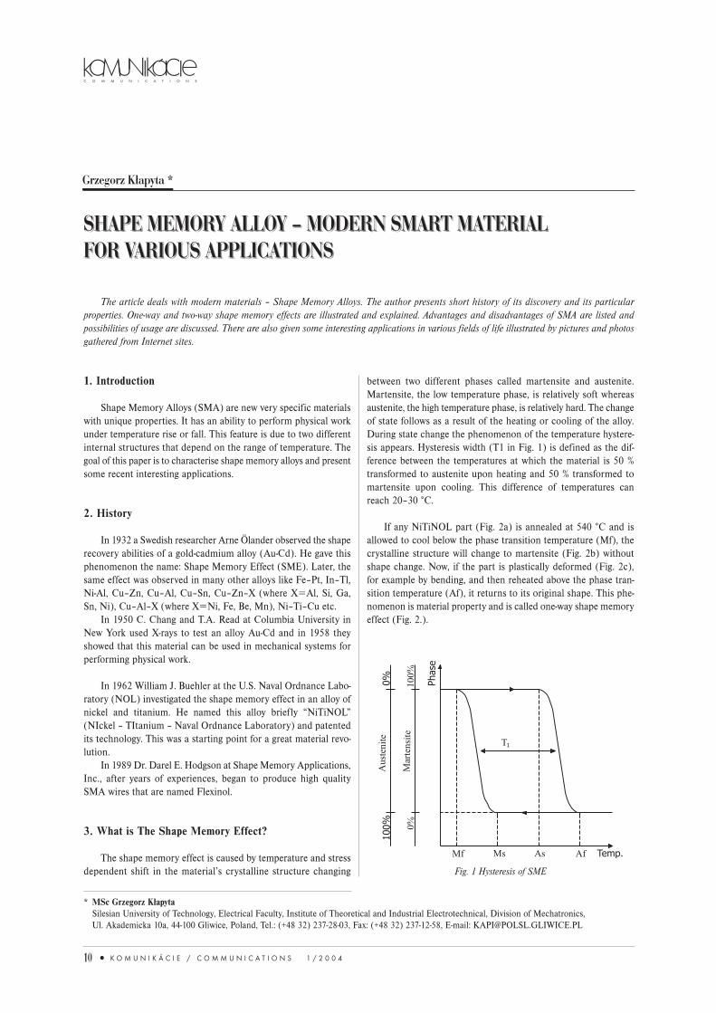


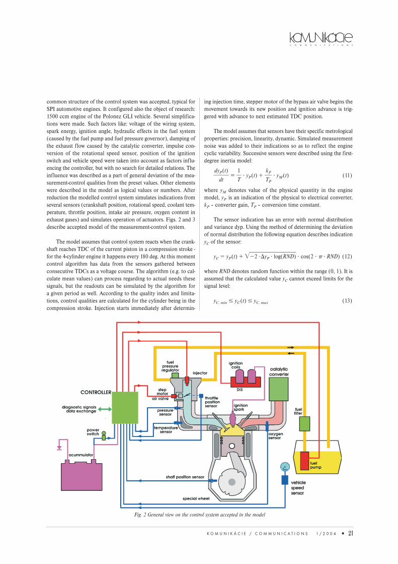

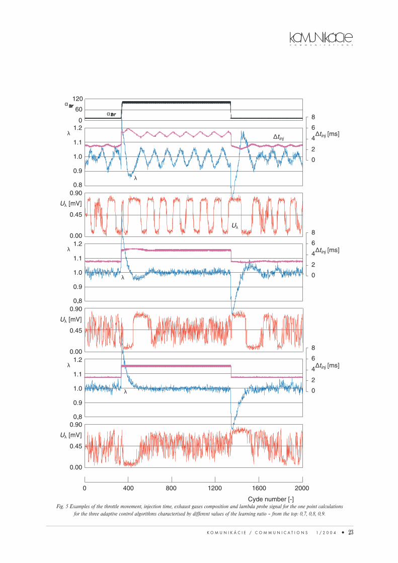


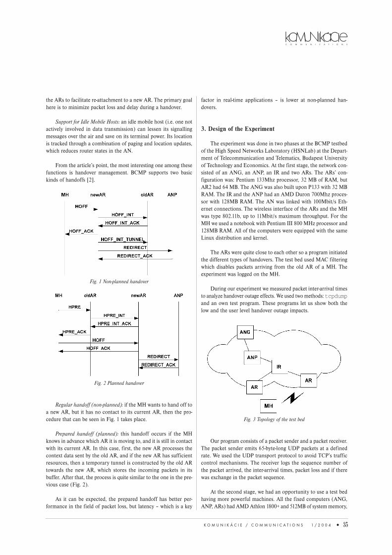


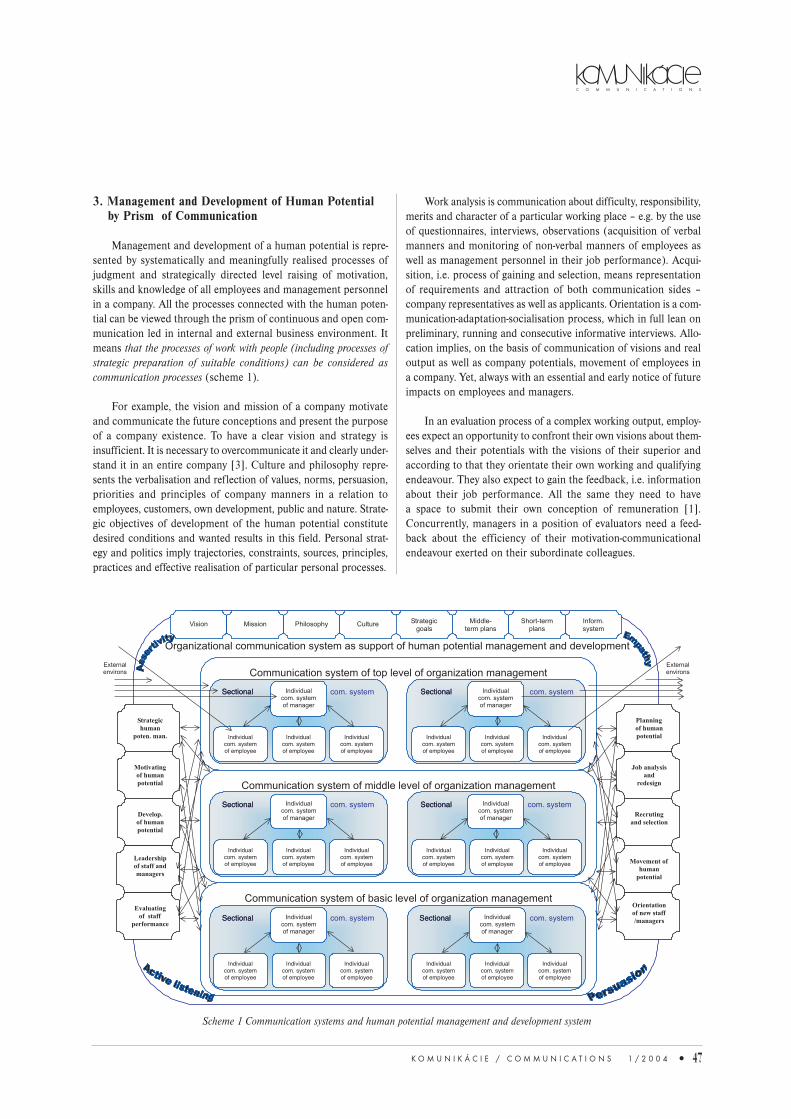


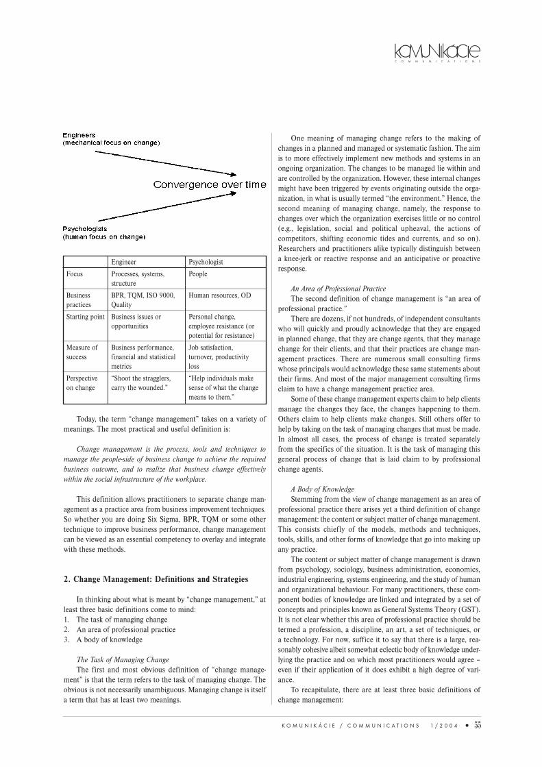


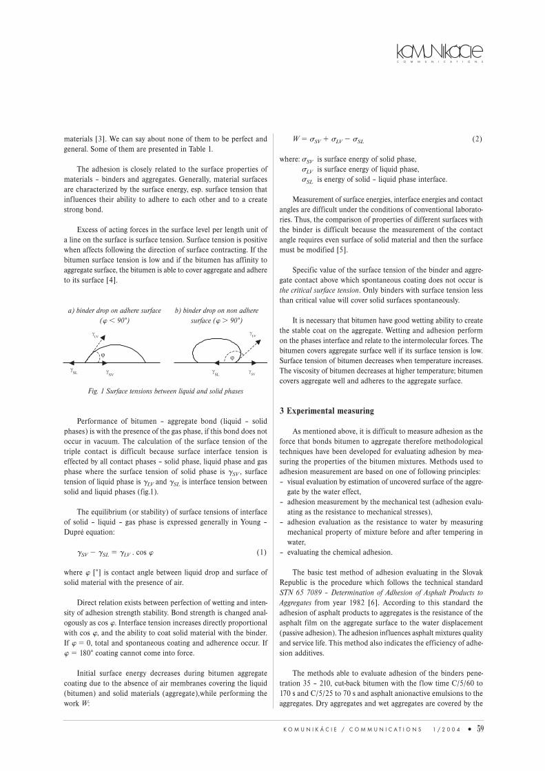


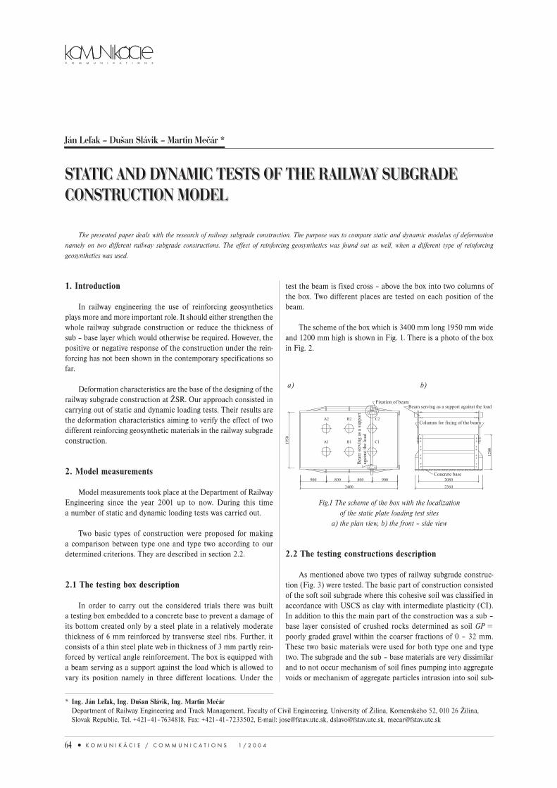


![C OMMUNIC A TIONS2005/04/04 · C OMMUNIC A TIONS K OMUNIKÁCIE / COMMUNICATIONS 2/2004 51. Introduction The HSDPA concept (High Speed Downlink Packet Access, e.g., [1], [2]) of UMTS](https://static.documents.pub/doc/80x56/5f9735d6b26a6e7d453e68bc/c-ommunic-a-20050404-c-ommunic-a-tions-k-omunikcie-communications-22004.jpg)


