49
Calculating the Market-Based Emissions- Intensity of Electricity Consumed in Australia SP0021
Calculating the Market-Based Emissions-Intensity of Electricity Consumed in Australia SP0021
Authors Philip Harrington, Strategy. Policy. Research.; Dr Hugh Saddler, Sustainability Advice Team.
Title Calculating the Market-Based Emissions-Intensity of Electricity Consumed in Australia
ISBN
Format
Keywords Renewable energy, greenhouse gas intensity, market-based intensity factors.
Editor
Publisher
Series
ISSN
Preferred citation

Report Template 2
Acknowledgements The authors wish to acknowledge the considerable support and assistance provided by the Project Steering Committee members:
• Dr Iain Macgill, Associate Professor, University of NSW
• Maria Balabat, Senior Lecturer, University of NSW
• Graham Sinden, Director – Climate Change and Sustainability Services, Ernst & Young
• Caitlyn Melia (Director) and Rachael Burgess (Director, Acting), National Inventory Team, Australian Government Department of the Environment and Energy
• Stewart Wallace, CRC for Low Carbon Living.
The project was delivered by:
• Philip Harrington, Principal, Strategy. Policy. Research
• Dr Hugh Saddler, Principal, Sustainability Advice Team.
Calculating the Market-Based Emissions-Intensity of Electricity Consumed in Australia – Final Report
Prepared for: Date:
CRC for Low Carbon Living March 2019
iv
Revision History
Rev No.
Description Prepared by Reviewed by Authorised by Date
00 Discussion Paper HS PH PH 31/8/2018
01 Exposure Draft Final Report
HS PH PH 16/1/2019
02 Final Report HS PH PH 13/2/2019
v
Table of Contents
Contents Executive Summary ........................................................................................................................................................................... 1 1. An Overview of the Problem ................................................................................................................................................ 2
1.1. Overview .............................................................................................................................................................................. 2 1.2. Background and NEM Context ............................................................................................................................................ 4 1.3. Objective and Timing ........................................................................................................................................................... 6 2. Accounting for Electricity-Related Greenhouse Emissions ...................................................................................... 7 2.1. Regional Approach .............................................................................................................................................................. 7 2.2. Market-based Approach ...................................................................................................................................................... 9 3. Defining the Market-based Methodology ..................................................................................................................... 13 3.1. System boundaries ............................................................................................................................................................ 13 3.2. Identification of supply sources ........................................................................................................................................ 13 3.3. Explicitly contracted sources ............................................................................................................................................. 14 3.3.1. Electricity supplied behind the meter from rooftop PV installed on-site ................................................................... 14 3.3.2. Electricity supplied behind the meter from other on-site generators, such as gas fuelled cogeneration ................. 14 3.3.3. Electricity supplied through a direct connection to an independently operated nearby generator, i.e. supplied “behind” the connection to the local network .............................................................................................................................. 15 3.3.4. Electricity acquired contractually through a GreenPower contract with a retailer .................................................... 15 3.3.5. Electricity acquired contractually through a Power Purchase Agreement with a grid connected generator, either renewable or fossil fuel .................................................................................................................................................................. 16 3.3.6. Large generation certificates (LGCs) purchased and cancelled, independently of electricity acquisition ................. 17 3.4. Residual supply and implicitly contracted sources ........................................................................................................... 17 3.4.1. Residual supply: Item 7, Large Renewable Energy Target cost ................................................................................... 18 3.4.2. Residual supply: Item 8, Small Renewable Energy Scheme cost ................................................................................. 19 3.4.3. Residual supply: Item 9, Remaining component ......................................................................................................... 20 4. Options for calculating the emissions intensity of “residual grid supply ........................................................... 21 4.1. Calculating at the whole system level ............................................................................................................................... 21 4.2. Alternative method: Use of the AEMO CDEII ................................................................................................................... 25 4.3. The issue of interconnector flows ..................................................................................................................................... 27 4.3.1. Queensland/NSW ......................................................................................................................................................... 29
NSW/Victoria ............................................................................................................................................................................ 29 4.3.2. Victoria/Tasmania ........................................................................................................................................................ 30 4.3.3. Victoria/SA .................................................................................................................................................................... 30 5. Choosing an ideal approach to calculate emissions intensity ............................................................................... 31 5.1. Defining the problem ........................................................................................................................................................ 31 5.2. Identifying feasible options ............................................................................................................................................... 34 5.2.1. Excluding the effect of EITE exemptions ...................................................................................................................... 34
vi
5.2.2. Use of a single NEM average emissions intensity ........................................................................................................ 35 5.3. Comparison of options ...................................................................................................................................................... 35 6. Other issues ........................................................................................................................................................................ 37 6.1. Marginal Loss Factors ........................................................................................................................................................ 37 6.2. Inclusion of small rooftop solar......................................................................................................................................... 37 6.3. Diurnal and seasonal variations in the emissions intensity of electricity consumed ...................................................... 39 7. Conclusions and Next Steps ........................................................................................................................................... 41
Index of Figures Figure 1: Moving annual net interconnector flows between states/regions in the NEM .................................................................. 28 Figure 2: Moving annual gross interconnector flows ........................................................................................................................... 28 Figure 3: Interconnector flows and total demand in SA ...................................................................................................................... 29 Figure 4: Emissions Intensity of Residual Supply Calculation Flow Diagram ...................................................................................... 33
Index of Tables Table 1: Shares of LRET accredited sent out renewable generation by state, 2016-17 ..................................................................... 31 Table 2: Sent out emissions intensity of residual supply in each state under the three options, 2016-17, in t CO2-e/MWh .......... 35 Table 3: Sent out emissions intensity of residual supply in each state under the three options, 2017-18, in t CO2-e/MWh
(preliminary values only) .............................................................................................................................................................. 36
Making the business case for sustainability 1
Executive Summary This report highlights that, at present in Australia, two different approaches to defining the greenhouse emissions associated with electricity consumption are being used by different parties and in different contexts. These are known as the regional and market-based approach. While both are valid and appropriate in different contexts, the use of the two by different parties, and without reconciliation or transparency, raises certain risks:
1. Non-recognition, in certain contexts, of the zero-carbon status of electricity consumption being paid for and consumed by certain parties, which may lead to economic losses for them;
2. The potential for double-counting of the emissions-benefits of renewable energy generation projects or output by different parties.
At the same time, there is an opportunity to define, and populate with available data, a market-based methodology for greenhouse gas emissions associated with electricity consumption. This approach – which would complement and not replace current regional-based accounting constructs – is consistent with international best practice as set out in the World Resources Institute’s GHG Protocol Scope 2 Guidance.
A transparent and well-defined market-based emissions accounting methodology may be better suited than the alternative (and current default) approach of regional emissions-intensity factors to the increasing scale and complexity of renewable electricity generation and trade in Australia, at least for some parties and in some circumstances. The tensions between the two approaches are perhaps best illustrated at present in the Australian Capital Territory (ACT), with the two generating vastly different observations of the emissions associated with electricity consumption in that Territory. However, the ACT only illustrates a particular example of a more general and growing phenomenon.
Indeed, it is timely to address these issues now, as there are expectations that the take-up of power purchase agreements (PPAs) will only continue to grow in Australia in future, driven by market fundamentals such as the increasing cost-effectiveness of renewable electricity generation. PPAs can also offer terms and conditions that are attractive to at least some consumers, and which may enable them to better manage electricity price risks.
The methodology and available data sets explored here may not provide a complete response to the issues described, and there may be a need for further work by the relevant agencies. However, we expect that this report provides a sound starting point and approach for addressing the issues. This Exposure Draft Final Report will be circulated to the project’s Steering Committee for further review and feedback, with a Final Report to be issued as soon as this occurs.
Ultimately, our aspiration is that this Report will assist governments and other parties to put in place effective arrangements to reduce the risks noted.
Making the business case for sustainability 2
1. An Overview of the Problem
1.1. Overview
This project addresses a rapidly-growing anomaly in the way that greenhouse gas emissions associated with electricity consumption are accounted for in Australia. The anomaly arises because of the increasing complexity in the ownership rights related to renewable electricity, and it is rapidly growing in extent and significance because of the increasing volume of renewable energy generation and trade in Australia.
To know the greenhouse gas emissions that are attributable to the consumption of a unit of (grid-based) electricity in a particular state or territory, for example, it is no longer sufficient to refer the state-/territory-wide emissions intensity average for the year in question. These averages are based primarily on the electricity generation mix within each state/territory (or, strictly, National Energy Market (NEM) region) and each year, with adjustment for interstate trade as measured by energy flows on the various interconnectors. However, the emissions induced by consumption by a particular consumer (or group of consumers) in a particular location can no longer be assumed to be the same as that implied by the generation mix in that state/territory because, increasingly, that consumption may be covered by a contract that guarantees delivery of 100% renewable electricity, but such contracts are not recognised in the ‘regional’ or state-based method of calculating greenhouse gas emissions.
In the case of the Australian Capital Territory (ACT), for example – which is not a region of the National Energy Market (NEM), but rather treated as part of the New South Wales (NSW) region – the consumption of grid-based power is attributed with generating emissions at the rate specified by the relatively-high NSW emissions average. However, the ACT Government holds renewable energy power purchase agreements (PPAs), or contracts, covering over 80% of the Territory’s total annual consumption, with this figure set to reach 100% by 2020. Taking these contracts into account, the greenhouse gas emissions associated with a unit of electricity consumption in the ACT are already very low and will soon be zero. However, under national emissions reporting schemes and at least some government programs, not only will these contracts be ignored, but the additional renewable generation they induce will be attributed as an emissions reduction benefit in the state/territory where the power was generated, and not in the state/territory that is paying for the investment.
The key issue highlighted in this Report is that, depending upon the context, the consumption of electricity by one consumer in the one location and at the one time can be associated with two different greenhouse gas emission observations: one based on a ‘regional’ approach (the state/territory annual generation intensity averages), and the second a ‘market-based’ approach, which recognises the particular contracts that different parties may hold.
Arising from this are two key risks:
Making the business case for sustainability 3
1. That the emissions benefit which a particular consumer is paying for may not be recognised, in certain contexts, in ways that create losses or other damage for the consumer;
2. That the emissions-abatement benefits associated with renewable electricity consumption may be double-counted.
On the first issue, and in an era in which carbon emissions are not explicitly priced, it may be thought that the potential confusion arising about the emissions attributable to a particular consumer is not material. However, a consumer’s legal obligations and entitlements may already be affected by their attributable emissions, at least in specific contexts. Reporting duties under the National Greenhouse and Energy Reporting (NGER) Act, for example, are based on triggers that include total emissions (and also energy production/consumption). The quantity of (Scope 2) emissions recognised for this purpose will depend on the accounting construct used.
Ratings under national ratings schemes, such as the National Australian Built Environment Rating Scheme (NABERS), are influenced by state/territory emissions averages (including the NSW electricity emissions average apply to buildings rated in the ACT). Doubtless for historical reasons, NABERS recognises Green Power purchases as emissions-free but does not recognise renewable energy PPAs. Eligibility for certain grants or other benefits may be affected by a person’s or entity’s emissions profile.
Beyond these direct implications, some consumers are paying premiums (but see below) to be supplied with 100% renewable electricity that is ‘additional’ to that which would have to be generated in any case, to fulfil the requirements of the large-scale renewable energy target (LRET) scheme. Some do this for ethical reasons, for reputational or branding reasons, or to meet local or international corporate policy requirements. In addition, with new renewable energy generation costs falling below that of other available sources, there is also a growing financial incentive for parties to contract for electricity with specific counterparties. However, these transactions are effectively not recognised in current greenhouse gas emissions accounting in Australia.
The ACT is only one example of the impacts that contracts can have on the emissions intensity of a particular consumer’s, or group of consumers’, electricity consumption. In recent years, the market for renewable energy PPAs has been growing rapidly, and not only because of the zero emissions footprint of the power. Increasingly, new renewable energy PPAs are being concluded at ‘below (wholesale) market’ prices, and with long terms that are otherwise unavailable in the NEM. For this reason, in particular, many commentators expect the volume of (renewable) electricity supplied under PPAs to increase rapidly in coming years. Therefore, there is the risk that confusion around the emissions accounting could grow, and it seems timely to address the issue now, before such confusion is too wide-spread.
Whether consumers are paying a premium or a discount for renewable energy, they are paying for certified renewable energy and we can be confident that the consumer will wish to have the renewable nature of their power supply arrangements recognised. They would not welcome being
Making the business case for sustainability 4
treated – under any law or government program – as if their emissions were in fact higher, simply as a function of their geographic location.
On the second issue – the risk of double-counting of the same renewable generation – if the ACT’s demand for renewable electricity, for example, is supplied, in part, from a wind farm in South Australia, it is very likely that both the selling and purchasing jurisdictions will claim emissions benefits from the same generation. To be clear, these claims are being made under two different accounting constructs, as is discussed in detail below, and no laws are being broken. However, the double-counting may occur all the same. Essentially this is because the ‘regional’ and ‘market-based’ approaches to emissions accounting are not reconciled with each other and, for the most part, the market-based approach is not being fully recognised.
1.2. Background and NEM Context
Before diving deeply into the specifics of this issue, and also before we propose a detailed methodology that could be used to account for market-based emissions and reconcile them with regional emissions factors, we should recall some context. The NEM is both a single interconnected physical system and a wholesale market in electricity traded across the system. A key feature of the design of the NEM is that the consumption and generation of electricity may occur in locations physically remote from each other, including in different (inter-connected) states.
The NEM is a ‘gross pool’ design, often described by analogy as a bathtub with a missing plug: provided that the amount of water flowing into the tub (generation) is matched by the volume flowing out of the tub (consumption) at all times, then a constant water height is achieved (reflected, in the NEM, by a (relatively) constant frequency of 50 hertz). Indeed, this dynamic balance must occur in all time periods for a stable power system. Provided this dynamic balance is achieved, it matters relatively little, from the perspective of the energy market, at which points in the system power is injected or removed – accounting for energy losses, of course, and for particular network constraints that may limit power flows between regions.
The gross pool design was intended to facilitate efficient pricing of wholesale electricity, as all power was and is required to be traded and settled through the one ‘clearing house’ (the Australian Energy Market Operator). This enables certain forms of price discovery; in particular, for short-term or spot prices. This approach is also consistent with the underlying physics of inter-connected grids, in that generation from any one unit on a grid is effectively blended with all other generation, subject, as noted, to physical constraints such as interconnector capacity. Linking generation from a particular unit to a particular consumer (on different sites) can be done, but only using contracts and financial instruments.
Also, from the initial design phase of the NEM, it was recognised that market participants would require financial contracts (‘hedges’) of various kinds in order to manage their risks in what was expected, and has proven to be, a volatile pricing environment. These are transactions that are separate from, but linked to, triggers or events in the pool, that are equivalent to insurance
Making the business case for sustainability 5
products. Hedges are highly varied in form and detail but are generally longer-lived contracts (one or two years). Retailers and generators typically hold a diverse and constantly-changing portfolio of hedges that balance risk-mitigation, on the one hand, with profit maximisation, on the other.
Further, and increasingly over time, the emissions-intensity, or ‘renewableness’ of specific electricity production and consumption was recognised as having additional and independent value from the value associated with the electrons supplied by renewable energy generators. Like a hedge, this value is traded separately from the energy market – sometimes referred to as the market for electrons. In particular, under what is now the LRET, large generation certificates (LGCs), equivalent to 1 MWh of certified renewable electricity, may be earned by renewable generators at the same time as they generate power. These certificates, however, can be sold to third parties – that is, parties not involved in the consumption of the electricity in question.
This history is reviewed firstly because it underscores that the problem highlighted in this paper is not new. It was always uncertain where a unit of generation would occur in response to a particular demand for electricity and, therefore, what greenhouse gas emissions would be caused. Initially this was considered of little import in the NEM. However, with the design of the then MRET (mandatory renewable energy target) in the late 1990s (now LRET), and its start in 2000, the value of low-carbon electricity was recognised. The development of renewable energy certificates (RECs), now LGCs, as separately tradeable instruments, was consciously done in order to facilitate the efficient development of the renewable electricity sector. The separation of RECs/LGCs from energy enabled- and still enables today – renewable energy generators to trade the ‘renewableness’ of their power with any party in the NEM, ensuring efficient competition between renewable energy suppliers, and therefore efficient pricing of renewable electricity.
The second reason for reviewing this history is to highlight that it has always been the case in the NEM, and it continues to be the case today (including with PPAs and other complexities), that the power actually consumed in given location may have been generated anywhere in the NEM, and this holds true regardless of whether the generation is renewable or otherwise. A PPA does not guarantee that the power consumed in a particular location was generated at a particular generation facility.
For example, if I am a university in NSW and I hold a PPA with a solar generator, also located in NSW, for the supply of (a certain volume of) renewable electricity, this does not mean that the power I consume will necessarily have been generated at that site. What it means is that the particular generator named in the paper (the solar farm) is required to supply a volume of LGCs in a year that is at least sufficient to cover the volume of energy contracted by the university. The solar farm can generate those LGCs by generating at any time and regardless of where the power is consumed. Indeed, it can and mostly will arrange its own hedges with other renewable energy generators, to ensure that it is able to manage any risk of shortfalls in its supply of LGCs. Since an LGC ultimately represents an additional MWh of renewable electricity, regardless of where that electricity is generated, then a PPA for a certain volume of renewable electricity simply makes the generator accountable for ensuring the outcome that the customer is paying for – that is, that a specific volume
Making the business case for sustainability 6
of additional renewable electricity is generated, somewhere in Australia, to cover their particular requirements, and on agreed terms.
1.3. Objective and Timing
It is timely to address the issues raised in this report now, as renewable energy generation and trade is growing rapidly, as is the use of PPAs. Parties holding PPAs, as noted, are likely to insist – in specific contexts – that their emissions footprint should take these legally-binding contracts into account. Identifying a methodology that would enable this outcome is the primary focus on this report. More and more companies, organisations, cities and even states and territories (notably, the ACT) are already accounting for their emissions and emissions abatement not on a location basis, but rather using a market-based method that takes into account the contracts they hold.
As is discussed below, it is feasible to reconcile emissions-intensity of electricity consumption on both regional and market-based constructs. However, this is not occurring at present in Australia and, as a result, we have two conflicting and mutually irreconcilable sets of emissions and abatement claims being made by different entities in Australia. The objective of this report is therefore the development of a clear, repeatable and rules-based methodology for market-based emissions accounting. We hope that such a methodology could be applied to reduce the risks associated with the use of these two accounting constructs.
Making the business case for sustainability 7
2. Accounting for Electricity-Related Greenhouse Emissions For most buildings and other energy using establishments in Australia, the largest source of greenhouse gas emissions associated with their operation is scope 2 emissions arising from the generation of the electricity used at or in the establishment. The exception to this generalisation is Industrial establishments which use gas or, in a minority of cases, coal or other fuels, to provide industrial process heat. These would be the minority of individual establishments or non-residential electricity consumers and therefore, for simplicity of expression, the remaining text assumes that the electricity using establishment is a building. The method is thus intended to be applicable to any type of establishment.
Some existing buildings (but probably few if any new buildings) generate electricity on-site in gas-fuelled cogeneration facilities. Owners/operators of such buildings report all emissions arising from on-site consumption of gas and any other fossil fuel used under scope 1, irrespective of the uses to which the energy services to which use of these fuels is (notionally) linked. If electricity generation is one of those services, then scope 2 emissions linked to the electricity generated and consumed on-site, i.e. behind the meter, are reported separately, but are not additional to the total scope 1 emissions. However, if any additional electricity is imported from the grid, then scope 2 emissions associated with these imports are additional. Similarly, if some of the of the cogenerated electricity is exported to another party, then that party reports the scope 2 emissions associated with the electricity it acquires from the first party. These reporting protocols ensure that all emissions are fully accounted for and that responsibility for those emissions can be correctly attributed to the party which is the end user of the energy associated with those emissions.
2.1. Regional Approach
Returning to the main topic of scope 2 emissions associated with electricity acquired for use in a building, the starting point is to note that these are calculated as the product of the quantity of electricity consumed, as measured by metered purchases, multiplied by the emissions intensity of that electricity. This method is specified for entities required to report their emissions under the NGER Scheme in Section 7.2, p. 301 of the National Greenhouse and Energy Reporting (Measurement) Determination 20081 in the following terms:
7.2 Method 1—purchase and loss of electricity from main electricity grid in a State or Territory
(1) The following method must be used for estimating scope 2 emissions released from electricity purchased from the main electricity grid in a State or Territory and consumed from the operation of a facility during a year:
1 http://www.environment.gov.au/climate-change/climate-science-data/greenhouse-gas-measurement/nger/determination
Making the business case for sustainability 8
where:
Y is the scope 2 emissions measured in CO2 e tonnes.
Q is the quantity of electricity purchased from the electricity grid during the year and consumed from the operation of the facility measured in kilowatt hours.
EF is the scope 2 emission factor, in kilograms of CO2 e emissions per kilowatt hour, for the State or Territory in which the consumption occurs as mentioned in Part 6 of Schedule 1.
Note: There is no other method for this section.
The NGERS Technical Guidelines,2 which are a comprehensive but somewhat more user-friendly interpretive expression of the Measurement Determination, go on to explain (p. 527) that EF is calculated as the sum of all emissions from power stations within a state, plus emissions associated with imports of electricity into the state, calculated as the quantity of electricity from each relevant state multiplied by the in-state emissions intensity of that electricity, minus emissions associated with exports from the state, calculated as the product of the total export volume multiplied by the in-state emissions intensity of generation. This calculated total emissions quantity is then divided by the sum of total electricity sent out from power stations within the state, plus the quantity of electricity imported, minus the quantity of electricity exported. The Technical Guidelines set out the complete algorithm for this calculation.
EF values are updated each year and are published in Schedule 1, Part 5 (p. 323 in the 2018 compilation) of the Measurement Determination, and are those specified, in a somewhat more accessible format, by the National Greenhouse Accounts Factors for the most recent available year, termed hereafter NGA Factors. 3 These are normally published in July or August each year, and, because of the unavoidable delays associated with input data availability, are calculated from data for the financial year ending in June of the previous year. Thus the current values, in the July 2018 edition of NGA Factors, are based on data for 2016-17. The NGER Technical Guidelines state, on p. 34 of the current edition, that:
The scope 2 emission factors are state-based emission factors from on-grid electricity generation calculated systematically from the physical characteristics of the electricity grid. The state-based emission factor calculates an average emission factor for all electricity consumed from the grid in a given state, territory or electricity grid. All emissions attributable
2 http://www.environment.gov.au/climate-change/climate-science-data/greenhouse-gas-measurement/publications/nger-technical-guidelines-reporting-year-2017-18 3 http://www.environment.gov.au/climate-change/climate-science-data/greenhouse-gas-measurement/publications/national-greenhouse-accounts-factors-july-2018
EFY = Q 1 000
×
Making the business case for sustainability 9
to a state territory or grid’s electricity consumption are allocated amongst individual consumers in proportion to their relative level of consumption. In effect, the likelihood of a particular generator supplying a particular consumer is assumed to reflect each generator’s relative level of supply to the grid. The reason for this approach is that within an electricity grid it is impossible to physically trace or control the actual physical source of electricity received by each customer.
This approach minimises information requirements for the system and produces factors that are relatively easy to interpret and apply, and which are used to support a range of specific government programs and policies. Consistent adoption of these ‘physical’ state-based emission factors ensures the emissions generated in each state are fully accounted for by the end-users of the purchased electricity and double counting is avoided.
It is recognised that this approach does not serve all possible policy purposes and that alternative, more data-intensive approaches are possible. Reporters will be able to provide additional data on a voluntary basis on consumption of certain renewable products.” (pp. 527-8)
The final paragraph quoted above is a succinct summary of the purpose of this project. Over the past year, the number of commercial and industrial electricity consumers entering into direct Power Purchase Agreements (PPAs) with renewable electricity generators has grown from a trickle to a substantial flow. Most of these agreements are with generators remote from the consumer – in many cases in different regions (states) within the National Electricity Market (NEM). This means that the physical supply of electricity will continue to be provided through the transmission grid and the local distribution network closest to the location of the consumer. However, the consumer has a financial contract with, and is therefore paying for, electricity supplied by the remotely located generator to the grid in its immediate neighbourhood. In other words, there is a separation between physical supply and contractual supply.
As noted in Chapter 1, this distinction has been a fundamental aspect of the operation of the NEM since its inception. Most large generators contract for much of their output with large consumers, including both retailers, which on-sell to mass consumers, and some large individual industrial and commercial consumers. Such financial contracts protect both generators and consumers from the worst of the large price fluctuations often seen in the spot wholesale market of the NEM. The only relevant attributes of the electricity being traded in these contracts are its price, its volume, and when the contracted volume is to be supplied, including hour of day, day of week and week of year. Other attributes, such as emissions intensity, are not normally considered.
2.2. Market-based Approach
However, even before the NEM started (in late 1998), it became apparent that some consumers wished to be able to consume emissions-free electricity. The GreenPower scheme was established in 1997 to meet the wishes of such consumers. Under GreenPower, electricity retailers contract
Making the business case for sustainability 10
with customers to supply zero emission electricity in quantities needed to supply part or all of their consumption. The retailers in turn enter into contracts with accredited zero emission generators in volumes sufficient to cover their contracted sales of zero emission electricity. Participating retailers are required to report quarterly on volumes sold and volumes purchased, and all parties are audited annually to ensure that purchases and sales are in balance. By virtue of these administrative processes, GreenPower consumers are able to claim, with a high degree of certainty, that some or all of the electricity they consume (depending of the terms of the contract with their retailer) is zero emission. On the other side of the contract, generators receive (at least until now) a premium price for their output, which the retailer recovers through higher prices charged to the consumer. In the last couple of years, the rapid reduction in the cost of new renewable generation has reduced the additional cost of zero emission generation, but, for consumers, has also made rooftop solar generation a more attractive option for electricity consumers wishing to reduce their emissions.
GreenPower certification enables consumers to set scope 2 emissions for that part of their electricity consumption supplied by GreenPower at zero. The residual part of their total consumption has, until now, been allocated the emissions intensity specified by the applicable NGA factor value. This project seeks to generalise from the specific example of GreenPower, with the aim of providing a method which can be used to calculate scope 2 emissions for all possible combinations of arrangements which consumers may use to acquire the electricity they consume.
The need for such a method was anticipated internationally by the World Resources Institute, in the Global Protocol for Community-Scale Greenhouse Gas Emission Inventories, released in 20144. This document is designed to be used by sub-national, and, especially, local, governments to prepare greenhouse gas emission inventories for their areas and does not apply to individual electricity consumers. Importantly, however it departs from the original Greenhouse Gas Protocol Corporate Accounting Standard5 in providing two distinct options for calculating scope 2 emission factors. In 2015, a further document, called GHG Protocol Scope 2 Guidance6, was released. This sets out for corporate entities, i.e. individual electricity consumers, more detail about the two options, called the location-based method and the market-based method. Under the location-based method, the relevant scope 2 emission factor is the average emission factor of the grid from which electricity is supplied to the reporting establishment. For Australia, this is functionally equivalent to the approach used to calculate the NGA factors. Under the market-based method, emissions factors are derived from contractual instruments, which include any type of contract between two parties for the sale and purchase of energy bundled with attributes about the energy generation, or for unbundled attribute claims. Markets differ as to what contractual instruments are commonly
4 https://www.wri.org/publication/global-protocol-community-scale-greenhouse-gas-emission-inventories 5 https://www.wri.org/publication/greenhouse-gas-protocol 6 https://www.wri.org/publication/ghg-protocol-scope-2-guidance
Making the business case for sustainability 11
available or used by companies to purchase energy or claim specific attributes about it, but they can include energy attribute certificates (RECs, GOs, etc.), direct contracts (for both low-carbon, renewable, or fossil fuel generation), supplier specific emission rates, and other default emission factors representing the untracked or unclaimed energy and emissions (termed the “residual mix”) if a company does not have other contractual information that meets the Scope 2 Quality Criteria. (p. 8)
The GHG Protocol Scope 2 Guidance specifies that reporting corporate entities should, to be compliant with the Greenhouse Gas Protocol Corporate Accounting Standard, report scope 2 emissions using both methods.
As can be seen from the quoted definition above, the Guidance document is necessarily very general regarding how to calculate a scope 2 market-based emission factor. The objective of this project is to define a much more explicit calculation procedure, which is applicable to Australian electricity market circumstances and could, in due course, be adopted as a universal method, to stand alongside the location-based emission factor calculated by the Department of Environment and Energy are specified in the Measurement Determination.
The general approach of the market-based method, as defined in GHG Protocol Scope 2 Guidance, follows five steps.
1) Define the boundaries of the system for which the calculation will be undertaken.
2) Identify all separate sources of electricity acquired and used by a consumer, where,under the market-based method, acquisition may mean a financial contract with agenerator, not physical supply of electrical energy from that generator, and determinethe quantities acquired from each source (activity levels).
3) Identify all such acquisitions which take the form of a payment, either explicit or implicit,per unit of electrical energy acquired.
4) Specify the emissions intensity of each of the sources which meet the criteria defined inboth steps (2) and (3).
5) For each such source, multiply activity (quantity of electricity acquired and paid for) byemissions intensity and sum the resultant emissions quantities across all sources.
In the following pages this report works through these steps in turn. The approaches to accounting and reporting set out in the Scope 2 Guidance document rightly place strong emphasis on data integrity and the importance of being able to document, in particular, claims as to the quantities of electricity acquired from various sources (activity data) and the emissions intensity of electricity supplied from those sources. This document provides detailed specifications as to data sources and documentation, which is particularly important because most of the parameter values input to the emissions calculation are calculated by the user, i.e. the reporting electricity consumer. In this respect, the market-based method differs significantly from the location-based method which

Making the business case for sustainability 12
uses an algorithm specified in the Measurement Determination, and an emission factor calculated by a government agency for use by all reporting entities.
The method is presented in the format appropriate for a single consumer (building or group of buildings and other establishments under common ownership and operational control). The initial discussion is framed in terms of calculating total annual emissions. The later part of this Paper discusses calculating over shorter time periods, which would be needed to identify seasonal and diurnal patterns.
Lastly, all the parts of the paper assume current policy settings. This includes taking account of the fact that the volume of wind and solar generation installed is likely to continue to grow for several years after 2020, beyond the quantity needed to meet the requirement of the Large Renewable Energy Target7.
7 http://www.environment.gov.au/system/files/resources/128ae060-ac07-4874-857e-dced2ca22347/files/australias-emissions-projections-2018.pdf
Making the business case for sustainability 13
3. Defining the Market-based Methodology
3.1. System boundaries
By far the largest electricity system in Australia is the National Electricity Market (NEM) grid, through which about 85% of electricity consumed in Australia is supplied. The other major system is the South West Interconnected System (SWIS) in WA, which supplies about 9% (both percentages depend somewhat on how the national total is defined). Other smaller systems include the North West Interconnected System covering the Pilbara region of WA, the Darwin-Katherine Interconnected System in the NT and Mount Isa in Queensland. There are also a number of small isolated systems, typically with only one major source of generation. Most of these are in WA, with smaller numbers in Queensland, the NT and SA.
The discussion in this Paper is largely confined to the NEM and the SWIS.
3.2. Identification of supply sources
The process of defining sources proceeds by identifying all sources which are contractually specific to the consumer, which is assumed to be network/grid connected. The quantities acquired from each identified source are then summed. If this sum is less than total electricity consumed, the balance of consumption (residual supply) is assumed to be acquired from the grid. The list of possible sources is intended to be comprehensive, and it is unlikely that any individual consumer will use all of the possible sources.
The list of sources is as follows.
1. Electricity supplied behind the meter from rooftop PV installed on-site.
2. Electricity supplied behind the meter from other on-site generators, such as gas fuelledcogeneration.
3. Electricity supplied through a direct connection to an independently operated nearbygenerator, i.e. supplied “behind” the connection to the local network.
4. Electricity acquired contractually through a GreenPower contract with a retailer.
5. Electricity acquired contractually through a Power Purchase Agreement with a gridconnected generator, either renewable or fossil fuel.
6. Large generation certificates (LGCs) purchased and cancelled, independently ofelectricity acquisition
7. Electricity paid for through the Large Renewable Energy Target cost component in astandard retail contract.
8. Deemed quantities of electricity generated and paid for through the Small RenewableEnergy Scheme cost component in a standard retail contract.
Making the business case for sustainability 14
9. Residual supply from the local distribution network in a standard retail contract.
Items 1 to 6 are all explicit contractual arrangements. Items 7 and 8 are arrangements which, because of the Renewable Energy (Electricity) Act 2000, as amended, form part of all standard retail contracts. They can therefore be considered as implicit contractual arrangements. Defining and determining/measuring both the emissions intensity and activity levels for items 1 to 6 is straightforward. Doing the same for items 7 to 9 is, by contrast, complex. We therefore discuss each of the two groups in turn.
3.3. Explicitly contracted sources
Each of the six listed sources is discussed in turn.
3.3.1. Electricity supplied behind the meter from rooftop PV installed on-site
Most suppliers of rooftop PV systems install inverters with a capability to report total generation, total consumption of energy imported from the local network, and total energy exported to the local network. If the system does not automatically provide total energy consumed by/in the building this can easily be calculated as: generation, minus exports, plus imports. The emissions intensity of this source is zero.
Behind the meter consumption from generation located on-site reduces the requirement for electricity acquired from another party and supplied through the meter or from a separate off-site source. It therefore does not need to appear in any part of the calculation of emissions intensity, or the subsequent calculation of total scope 2 emissions. However, every consumer will want and need to include behind the meter consumption when monitoring and analysing their total electricity consumption.
3.3.2. Electricity supplied behind the meter from other on-site generators, such as gas fuelled cogeneration
As previously noted, given the relative costs of gas and installed PV, there are unlikely to be any new installations of this kind in buildings, though there may be some at industrial sites with requirements for moderate to high temperature thermal energy. The host building/site would report emissions arising from a facility of this type under scope 1. The organisation will, however, need to have documentation, probably in the form of electricity retailer bills, showing energy imported and exported (if any). It is assumed that the cogeneration installation will monitor and record total electricity generation.
As with source 1, any behind the meter consumption would have the effect of reducing through the meter consumption, and therefore will not need to appear explicitly in the calculation.
Making the business case for sustainability 15
3.3.3. Electricity supplied through a direct connection to an independently operated nearby generator, i.e. supplied “behind” the connection to the local network
Documentation of any volumes of electricity falling into this category will take the form of bills from the supplying generator.
Calculation of scope 2 emissions from any electricity supplied from this source would have to be based on emissions intensity, as advised by the supplier. The most important question is how best to verify the advised emissions intensity figure. For a renewable supplier, this could be readily achieved by ensuring that the supplier is a renewable energy power station accredited under the LRET.
If supply is from a non-renewable source, such as an adjacent gas-fired cogeneration installation, emissions-intensity would have to be supported by a statement from the supplier of the sent out emissions intensity, supported by some form of auditable documentation. The most appropriate source for this would be the generator’s most recent NGERS report, as accepted by the Clean Energy Regulator. Regulatory and/or legislative changes may be required to ensure that the purchaser of such electricity can have full access to the relevant parts of the supplier’s NGERS report without breaching the strict commercial confidentiality protections applying to NGERS reports. If the supplier is not required to report under NGERS, it should be required to report to the purchaser that part of its energy use and emissions relating to the electricity, using the relevant NGERS reporting guidelines, and to submit the report to independent verification.
3.3.4. Electricity acquired contractually through a GreenPower contract with a retailer
Most retailers offer a range of GreenPower products which differ mainly in the fraction of accredited and audited zero emission electricity included contractually in each unit of electricity supplied. Thus, even if the total supply of renewable electricity is not itemised in each monthly bill it can be easily calculated from the total billed electricity supply. Note that purchases of GreenPower have been declining for many years. In 2017, total sales were 76% below the peak level, which was achieved in 2009, and accounted for less than 0.3% of total national electricity sales. The fall in GreenPower sales to commercial consumers has been even steeper – 81% from the 2009 peak8. The reasons for this decline are unclear, but it seems likely that a combination of other, more direct options for large consumers to acquiring zero emissions electricity supply, and, for small electricity consumers, the low cost of rooftop solar, have contributed. When established, roughly two decades ago, GreenPower was a pioneering scheme, and the only realistic option for consumers to actively
8 Data extracted from GreenPower Annual Audit and compliance Reports https://www.greenpower.gov.au/About-Us/Audits-And-Reports/
Making the business case for sustainability 16
reduce the emissions intensity of the electricity they used. It seems likely that the product is now nearing the end of its useful life.
The emissions intensity of GreenPower is zero and this is assured by the GreenPower accreditation and auditing processes.
3.3.5. Electricity acquired contractually through a Power Purchase Agreement with a grid connected generator, either renewable or fossil fuel
The quantity sent out from the contracted generator and charged to the purchasing party will be specified in invoices issued. However, uncertainties arise about how to treat transmission and distribution losses. If it were argued that, notionally, electricity is assumed to flow from the generator all the way to the consumer’s premises, losses might be quite large. However, in terms of real physics, the electrical energy generated will mostly flow to consumers close to the location of the contracted generator, meaning that actual losses will be smaller. We return to the question of losses later in the Paper.
Note that in order for this electricity to count towards the consumer’s supply of zero emission electricity, the contract must specify that payment is for both “black” and “green” components of the generation, i.e. for the electrical energy, and the Large Generation Certificates (LGCs) associated with that quantity of renewable electricity, and the LGCs must be cancelled (voluntarily surrendered). If the LGCs were not surrendered, but on-sold, they would have the effect of displacing renewable electricity which would otherwise have been generated to meet the LRET, thereby reducing the total quantity of renewable electricity generated. In effect, both the electricity and the LGCs must be “consumed” at the same time, if supply under the PPA is to count as renewable.
In the case of a renewable generator, the consumer should ensure that the PPA is with an LRET accredited generator. It can be reasonably assumed that, until 2020, all renewable generators will be LRET accredited, since that is the requirement for being able to generate, and earn revenue from, the sale of LGCs, as well as electricity. In the case of a non-renewable generator, the issues and associated questions are the same as those arising in relation to Source 3.
In the case of a contract with a non-renewable generator, the consumer should obtain from the supplier a statement of its sent out emissions intensity, as recommended above for similar behind the meter supply.
The approach proposed here assumes that, not only will the Clean Energy Regulator (or any successor body) continuer to accredit renewable generators and audit LGCs required to meet the ongoing LRET target out to 2030, but will also perform the same function for renewable generators which do not participate in the LRET, assuming continued growth in renewable generation capacity beyond that needed to fulfil the LRET.
Making the business case for sustainability 17
3.3.6. Large generation certificates (LGCs) purchased and cancelled, independently of electricity acquisition
An electricity consumer may purchase LGCs in the open market, independent of purchase of electricity. If the certificates are then cancelled, the certificates are not available to a liable party under the legislation, meaning that additional renewable generation will be required. The net effect, therefore is that the consumer is purchasing accredited zero emission electricity in MWh quantity equal to the number of certificates bought and cancelled. To put it another way, a quantity of standard “black” electricity purchased through a standard retail contract is converted to zero emission electricity. Documentation of the number of certificates bought and cancelled will be required.
The Clean Energy Regulator operates a rigorous certificate validation process and the REC Registry of LGCs appears to always contain a number of certificates which have been rendered “Invalid due to audit”9. It follows that each valid LGC is, by definition, equivalent to 1 MWh of zero emission electricity.
3.4. Residual supply and implicitly contracted sources
Any consumer wishing to claim one hundred percent zero emission supply of electricity must source their entire supply from some combination of the above six sources. However, a consumer moving towards one hundred percent will also be using some residual grid supply and will therefore wish to know the emissions intensity of this supply.
The total volume of residual supply is the difference between total electricity consumed and the sum of quantities of electricity supplied from each of the sources listed above. This will be calculated as:
Total supply through the meter
minus GreenPower purchases (if any)
minus PPA purchases (however defined)
minus Number of LGCs purchased and cancelled
minus Exports through the meter
As already explained, residual supply, for the purpose of calculating emissions using a market-based approach, consists of three distinct components, listed as items 7 to 9 above. We discuss each in turn.
9 http://www.cleanenergyregulator.gov.au/RET/Scheme-participants-and-industry/Power-stations/Large-scale-generation-certificates/Creating-and-registering-large-scale-generation-certificates/Large-scale-generation-certificate-validation
Making the business case for sustainability 18
3.4.1. Residual supply: Item 7, Large Renewable Energy Target cost
Activity level
Liability to pay for Large Generation Certificates (LGCs) is calculated as the quantity of electricity acquired from the network/grid, multiplied by the Renewable Power Percentage (RPP) for the applicable year. The LRET operates on a calendar year basis and the legislation requires the Clean Energy Regulator to announce the RPP for each year by 31 March in the year concerned10. The RPP for calendar year 2018 was announced on 29 March and is 16.06%. The main parties liable to pay for LGCs are the retailers, and they recover the cost through a (relatively small) component of their total retail prices. Thus a consumer pays a small premium on every kWh acquired through the grid to cover the retailers’ expenditure on buying LGCs. This is perhaps best thought of as a premium which makes the quantity of electricity represented by the number of LGCs renewable electricity, rather than “ordinary” fossil fuel grid electricity. In this respect this is very similar to the GreenPower premium, and it is for this reason that it can be considered part of the renewable electricity supply.
Liability for LGCs applies to all electricity acquired through the grid/network, and therefore also includes contracted supply through a PPA, because such supply passes through the grid/network. The PPA contract will include a component to pay for the LGC liability. Hence the quantity of electricity acquired from the network/grid, as specified above, is equal to residual network purchases, as defined above, plus purchases though a PPA, plus GreenPower purchases (if any). The renewable component of this acquisition is equal to the total quantity multiplied by the RPP. Some consumers, classified as those undertaking Emissions Intensive Trade Exposed (EITE) activities, are exempted from LRET liability for a fraction of their total electricity consumption, the fraction being specified by the Clean Energy Regulator.
Emissions intensity
Emissions intensity for most of this electricity is zero and automatically verified as such through the LRET procedures. However, in each year until 2020 (the LRET legislation is based on calendar years, not financial years), the total target includes 850 GWh reserved for electricity supplied by a small group of power stations which use waste coal mine gas (WCMG) as fuel. In 2020 the full target is 33,000 GWh for renewable generators and 850 GWh for WCMG generators. The eligibility of waste coal mine gas power stations to earn LGCs ends after 2020. Hence, in every year from 2021 until 2030, when the legislated program terminates, the annual target is 33,000 GWh of renewable electricity. What all this means is that until the end of 2020 the average emissions intensity of electricity paid for through the LRET cost component is slightly higher than zero.
There are currently seven WCMG power stations registered under the LRET legislation, and extremely unlikely to be any more. These power stations are Glennies Creek, Tahmoor, Teralba and
10 http://www.cleanenergyregulator.gov.au/RET/Scheme-participants-and-industry/the-renewable-power-percentage
Making the business case for sustainability 19
West VAMP (Ventilation Air Methane Power, located at the Westcliff colliery) in NSW, and German Creek, Moranbah North and Oaky Creek in Queensland. Two of these, Teralba and West VAMP are no longer operating. The other five generated in total 1,146.2 GWh in 2017-18, according to the NGERS Designated Generation Facilities public report 11 , which is based on financial year data provided by entities liable to report. However, some of the electricity generated by each of these plants is used within the plant for various auxiliary functions. This means that energy sent out is less than energy as generated, and it is sent out energy which determines the number of certificates generated. Sent out energy for all generators is treated as commercially confidential. We have estimated, using AEMO default auxiliary factor values, that energy sent out by these five generators was 1,044 GWh. The REC Registry shows that in calendar year 2017 there were 849,996 certificates generated by registered WCMG power stations, meaning that the 850,000 MWh target was effectively fully met.
We suggest that the average emissions intensity of electricity paid for by consumers through the LRET component be calculated as follows:
Total scope 1 emissions from all registered WCMG power stations in kt
divided by Total generation sent out from all registered WCMG power stations in GWh
multiplied by 850 GWh
divided by applicable LRET target for the year
Ignoring temporarily, for simplicity, the difference between financial and calendar years, and also the distinction between as generated and sent out, the calculation for 2018 would be:
(556.8 / 1,044.2) x (850 / 27,534.7) = 0.0165 t CO2-e/MWh
3.4.2. Residual supply: Item 8, Small Renewable Energy Scheme cost
Small Technology Certificates (STCs) are based on the deemed output of a small PV system (defined in the legislation s being a system of less than 100 kW capacity) over the period from the date of installation until 2030, based on capacity and location. They also cover electricity deemed to be displaced by solar and heat pump water heaters. Since certificate numbers are not based on actual renewable electricity generation, consumer payments for STCs should be viewed as a size (capacity) linked subsidy to support installation of rooftop PV and low emissions water heaters, not a payment for renewable electricity generation. As such, they should be excluded from the list of electricity supply sources.
11 http://www.cleanenergyregulator.gov.au/NGER/National%20greenhouse%20and%20energy%20reporting%20data/electricity-sector-emissions-and-generation-data/electricity-sector-emissions-and-generation-data-2016-17
Making the business case for sustainability 20
3.4.3. Residual supply: Item 9, Remaining component
The volume supplied under this item, i.e. the activity level, is equal to the total residual supply, as defined in Section 6 above, minus the LRET component, as also defined in Section 7 above. This is a very simple calculation for an individual consumer because it is, as the name indicates the residual component of electricity supplied through the meter, defined as:
Total residual supply
minus LGC liability related to total supply
Calculating the emissions intensity of this supply, however, is, as will be seen, far from easy, and most of the remainder of this paper explores various options for doing so. In the next chapter, we first examine how emissions intensity might be calculated at whole of system level, i.e. as a single average value for the NEM, or the SWIS as a whole. We then examine the feasibility of disaggregating the calculation to the level of NEM regions, i.e. the five separate states making up the NEM, recognising that this is the level at which the location based emissions intensity is currently calculated.
Making the business case for sustainability 21
4. Options for calculating the emissions intensity of residualgrid supply
4.1. Calculating at the whole system level
The general approach to calculating the volume weighted emissions intensity of electricity supplied by an electricity supply system or grid is as follows:
Volume weighted average emissions intensity is equal to:
sum of total emissions from identified power stations
divided by sum of total electricity sent out from identified power stations
This is the approach which AEMO uses each day in calculating its Carbon Dioxide Equivalent Intensity Index (CDEII) for electricity supplied each day in the NEM12. The calculation is undertaken for each NEM region and for the NEM as a whole.
Since the primary objective of the method being developed is to enable annual reporting of market-based scope 2 emissions, residual emissions intensity needs to be calculated on an annual basis. Calculating the volume weighted annual average emissions intensity of “residual” NEM generation is most easily understood as a series of steps.
Step 1 : Identify power stations to be included
For the NEM, AEMO publishes, and updates at regular intervals, a list of registered generators13. The list includes both the large grid connected generators and a great many of the small generators embedded within distribution networks. Many, but by no means all, of the latter are renewable, e.g. landfill gas. The obvious starting point for defining the power stations to be part of the residualsupply is to include all fossil fuel generators which are registered as market participants in the NEMor the SWIS, as applicable. However, this list will then need to be adjusted by both additions andremovals.
The main addition will be so-called below baseline generation by pre-LRET hydro generators. When the LRET started, in January 2001, there was a significant amount of hydro generation in all four eastern states. By far the largest amount of electricity being supplied by hydro was from large power stations in Tasmania, in the Snowy scheme in NSW, and in the Kiewa scheme in Victoria. There were also two power stations in far north Queensland and a number of much smaller embedded generators at storage reservoirs, most of which were in NSW and Victoria. For each of
12 http://www.aemo.com.au/Electricity/National-Electricity-Market-NEM/Settlements-and-payments/Settlements/Carbon-Dioxide-Equivalent-Intensity-Index
13 http://www.aemo.com.au/Electricity/National-Electricity-Market-NEM/Participant-information/Current-participants/Current-registration-and-exemption-lists
Making the business case for sustainability 22
these generators the LRET legislation defines a so-called baseline level of generation, originally related to their average level of output during the 1990s, but in some cases amended from time to time over the years since then. The LRET legislation allows any one of these “old” hydro generators, which is able to increase its output above the baseline level, to earn LGCs on generation above the baseline level. This provision was intended to provide the owners of “old” hydro generators with a financial incentive to make investments, such as turbine upgrades, which would enable them to increase their generation efficiency.
The consequence of this provision is that all below baseline generation from “old” hydro generators should be included in the calculation of residual supply, while any above baseline generation goes into the national “pool” of LRET supply. In doing so, some design details will need to be resolved. For example, should below baseline hydro generation be defined on a year by year basis, or on a multi-year moving average basis, given that total generation levels change quite markedly year by year, depending on a variety of factors, including water availability and the price of LGCs. The ACT uses a five-year moving average as the basis for its calculation of the emissions intensity of its electricity supply, but this may not be appropriate on a national basis because of the way it would interact with the calculation of LRET generation.
On the other side of the ledger, until after 2020, part of the output from the five currently operating WCMG power stations will have to be moved out of the residual category, into the LRET category. As already explained, the LRET total target each year includes a component of 850 GWh, i.e. 850 thousand LGCs, which is reserved for output from accredited waste coal mine methane generators. There are currently seven of these: Glennies Creek, Oaky Creek I and II, Tahmoor, Moranbah North, Teralba, and Westcliff, of which, as previously noted, Westcliff and Teralba are not currently operating. NGERS data shows that the first five generated a total of 1,146.2 GWh in 2016-17. Thus 1,146 - 850 = 296 GWh from these generators should be included in the residual category, because, while covered by the LRET, they are not zero emission generators.
The third qualification concerns grid connected cogeneration facilities, as previously mentioned. The AEMO registered generators list includes five such plants, all with a capacity of 1 MW or less. The associated list of exempt [from registration] small generators includes a further fifteen such facilities, all of which are exempt on the basis that they are smaller than 5 MW and export less than 20 GWh (about 0.01% of total NEM supply) in any 12 month period. The NGERS list of designated generation facilities includes 23 generators which appear to be cogeneration facilities. However, less than half of these appear on either the AEMO registered generators or the AEMO exempt list, suggesting that the majority do not export electricity at all. This is a presumption only, because there is no publicly available data on quantities supplied to local networks by any of these small facilities. We conclude from both the lack of data and from this rather confusing overlap of listings in some cases, and lack of overlap in other cases, that the total quantity of electricity exported into local networks from these gas-fired cogeneration facilities is negligibly small, relative to total generation. Consequently, excluding them from the calculation of emissions intensity is necessary
Making the business case for sustainability 23
on the practical ground that the required data are not publicly available, but will cause no significant distortion of the emissions intensity calculation.
This would conform with the approach used by AEMO to calculate its daily CDEII, which excludes all small non-market generators from its calculation.
In conclusion, therefore, the list of power stations to be included in the calculation of residual emissions intensity consists of:
all fossil fuel generators trading in the NEM
plus below baseline generation from “old” hydro generators
minus generation from accredited waste coal mine methane generators up to a maximum of 850 GWh per year until 2020.
Step 2: Determine total annual emissions from identified fossil fuel power stations
The best source of data for emissions is the annual Greenhouse and energy information for designated generation facilities prepared and published by the Clean Energy Regulator, based on NGERS returns by generators14. These data are published on a financial year basis, on the last day of February following the end of the financial year to which they relate, i.e. with a lag of precisely 8 months.
The NGERS data provide total annual emissions emitted by all power stations trading in the NEM, calculated on the strict principle of no double counting of emissions. Determining total emissions is therefore a simple matter of summing the reported emissions from all of the power stations identified in Step 1. This will include all emissions from the waste coal mine methane generators discussed above, even though not all of the electricity sent out from these generators will be included, for the reason described there.
Step 3: Determine annual electricity sent out from identified fossil fuel power stations
Generation data for individual power stations are available from the NGERS report. They are also available, with a much smaller lag, either direct from AEMO, in a format requiring a considerable amount of manipulation to be user friendly, or through a third-party service, such as NEM Review, which processes the raw AEMO data.
The key challenge in making the data from either of these sources useful for this project is converting from electricity generated to electricity sent out, i.e. determining what auxiliary load factor to use for each power station. This is a challenge, because measured electricity sent out from a power station, as opposed to electricity generated by the same power station, is commercially sensitive, and therefore not published, except in highly aggregated form, such as total dispatch.
14 See note 12 above.
Making the business case for sustainability 24
It is therefore necessary to use a set of specific auxiliary factor numbers for each power station to convert actual as generated figures to estimated actual sent out. In preparing its annual National Electricity Forecasting Reports, AEMO has to make the opposite conversion – from modelled consumer demand inclusive of transmission and distribution losses to modelled as generated energy. It uses for this purpose a set of standard auxiliary factor values which were originally developed for use in preparing its annual National Transmission Network Development Plan15. These values were originally sourced from a report commissioned from ACIL Allen in 2016, and subsequently published by AEMO16. However, AEMO has now published the relevant numbers in a much more convenient workbook format, containing all of the input assumptions used to prepare its Integrated System Plan17. It should be noted that AEMO does not use these values, which may vary slightly from year to year, when calculating its CDEII, as it has access to the metered sent out electricity from each power station on a continuous basis, because these data are integral to its role as the market operator. See the next section for more about the CDEII.
The AEMO input data workbook also contains a set of generic as generated emission intensity values for each power station. Scope 1 combustion emission factors are shown and also Scope 3 emission factors, mainly related to upstream fugitive emissions associated with the extraction of coal and gas. These scope 1 values, which are also derived from a report commissioned from ACIL Allen, could be used as an alternative to the values calculated from the NGERS data each year. If used, this source of emissions data would have to be used in conjunction with generation data sourced from the AEMO data system, as described above.
This approach, because the values are generic, would remove the need for annual recalculations. However, this very reality would make the approach less accurate, as the emission values would not be explicitly linked to power station operation in one actual year. The approach would also remove any relationship with the NGA factors for electricity, since these are based on actual year by year emissions as calculated for the National Greenhouse Gas Inventory. A further disadvantage of using the AEMO data is that this source does not include power stations outside the NEM, whereas the NGERS data includes all power stations, including those in the SWIS and the NT (though it may be hard to get auxiliary factor values for generators outside the NEM).
15 http://www.aemo.com.au/Electricity/National-Electricity-Market-NEM/Settlements-and-payments/Settlements/Carbon-Dioxide-Equivalent-Intensity-Index 16 https://www.aemo.com.au/-/media/Files/Electricity/NEM/Planning_and_Forecasting/NTNDP/2016/Data_Sources/ACIL-ALLEN---AEMO-Emissions-Factors-20160511.pdf 17 http://www.aemo.com.au/Electricity/National-Electricity-Market-NEM/Planning-and-forecasting/Integrated-System-Plan
Making the business case for sustainability 25
As previously noted, public NGERS data for each financial year are published on or before 1 March of the following year. It is recommended that NGERS data be used as the source for annual generation and emissions of individual power stations.
Step 4: Add below Baseline generation from “old” hydro generators
For each “old” hydro generator, the quantity of generation forming part of residual generation in the relevant region is equal to whichever is the less of the LRET Baseline for the relevant year of the quantity actually generated and the Baseline for that year. Note that, in doing the calculation for each NEM region, Snowy power stations are divided between Victoria and NSW. Murray 1 and Murray 2 are part of the Victorian region, while Tumut 1, Tumut 2, Tumut 3 (Talbingo), Blowering, and Guthega are part of the NSW region.
Step 5. Calculate volume weighted average emissions intensity of residual generation in each NEM region and SWIS and DKIS
For each power station in each year, sent out energy is equal to:
as generated energy
multiplied by (1 - auxiliary factor)
For each state/NEM region in each year, sent out electricity and total emissions are then summed across all identified generators in the state/region, to calculate the volume weighted emissions intensity of all generation in the region, as set out at the beginning of this Section. Note that total electricity generation will include below baseline generation by “old” hydro generators.
4.2. Alternative method: Use of the AEMO CDEII
As explained above, AEMO calculates and publishes its CDEII each day for each NEM state/region, using a procedure essentially identical to that described in the previous section. The key difference is that AEMO uses different input data, particularly for sent out generation. For the reasons explained, the AEMO data is certain to be more accurate than the public data proposed to be used in the method described above. As also explained, the AEMO calculation uses essentially the same sets of generators in each state as are proposed to be used in the calculation described above.
The key difference is that the AEMO calculation includes generation by all the LRET accredited generators, including both those generating LGCs, those supplying GreenPower, and those contracted through separate PPAs, of which the most important currently are the wind generators located in NSW, Victoria, and SA, but contracted by the ACT government. Another important difference is that the AEMO emissions estimates include scope 3 as well as scope 1 emissions18.
18 ) According to a statement by the Clean Energy Regulator which appears at the head of the first page of the Designated Facilities workbook for 2016-16: http://www.cleanenergyregulator.gov.au/NGER/National%20greenhouse%20and%20energy%20reporting%20data/electricity-sector-emissions-and-generation-data/electricity-sector-emissions-and-generation-data-2016-17

Making the business case for sustainability 26
Scope 3 emissions from electricity generation are mainly fugitive emissions arising from the extraction and processing of coal and gas supplied to power stations. It would not be consistent with the overall approach proposed in this study to include scope 3 emissions.
That said, for completeness, we set out a process for using the CDEII data to calculate the emissions intensity of residual electricity supply. The exercise is facilitated by the fact that the published daily data includes not only the average emissions intensity, but also estimated total emissions and total electrical energy sent out from all the generators in each state.
The requirement for this project is a single average annual residual generation emissions intensity value for each state. The calculation process which would be used is set out as a series of steps.
Step 1. Sum daily AEMO total state sent out generation and emissions across all days in the year
AEMO publishes what it calls its summary results as a single csv file for each calendar year19. Calculating an annual total is simply a matter of summing the relevant numbers for each day in the year concerned. The publishing lag is less than two weeks, so there will be no difficulty in calculating the required figure for the most recent financial year.
Step 2. Identify generators to be excluded from the calculation
AEMO publishes a list of all generators included in its calculation20, so it will be a simple matter to identify the accredited renewable generators, and the five WCMM generators to be excluded.
Step 3. Calculate electricity sent out during the year by excluded generators and subtract from total generation
This will be done using the same approach and sources used to calculate annual sent out energy under Step 4 of the procedure described above. Uncertainties associated with the need to assume auxiliary factor values will be very small because auxiliary factors for solar and wind generators are very small. AEMO uses 1% for all wind and solar (and hydro) generators.
Step 4. Make appropriate adjustments, as required, for “old” hydro and WCMM generators
The performance of these two sets of generators is assessed on an annual basis against their respective threshold values: individual annual LRET baselines for the “old” hydro generators and 850 GWh for the WCMM generators. Whether or not it will be necessary to make an adjustment to the annual total generation figure, additional to the adjustment described in Step 3, above, will be determined using the procedures described under Step 5 in section 5 above.
19 http://www.aemo.com.au/Electricity/National-Electricity-Market-NEM/Settlements-and-payments/Settlements/Carbon-Dioxide-Equivalent-Intensity-Index 20 See note 16 above
Making the business case for sustainability 27
Step 5. Divide AEMO total emissions by adjusted total generation to obtain emissions intensity of residual generation
This final calculation is the same as that used for the other method.
In conclusion, the fact that the emissions factors used to calculate the CDEII include Scope 3 emissions means that it is not an appropriate basis for the method, which should be confined to Scope 1 electricity generation emissions only. However, it may be helpful to use the CDEII method as a consistency check when doing annual calculations of residual emissions intensity
4.3. The issue of interconnector flows
The preceding sections have discussed options for calculating the average emissions intensity of residual electricity sent out from all relevant power stations in the NEM. An identical calculation could be done for each state/NEM region based on the generators located within the state. However, that is not equal to average emissions intensity of electricity supplied to consumers within any of the five NEM regions, because there are substantial flows between regions through interconnectors between each state transmission grid. The result is that in some regions total (residual plus LRET and other contracted renewable) generation exceeds consumption, in others consumption exceeds generation, and in others again the two are close to balance. Moreover, these relationships vary quite significantly over time.
There are four sets of interconnectors, as follows:
• between Queensland and NSW, a large capacity AC link, located between the Northern Tablelands of NSW and the Darling Downs in Queensland, and a smaller DC link located on the coast, near Coolangatta;
• between NSW and Victoria, three AC links: through the Snowy scheme, near Albury-Wodonga, and near Mildura;
• between Victoria and SA, one AC link in the south, and one smaller DC link in the north (of Victoria) between Mildura in Victoria and Renmark in SA; and
• between Victoria and Tasmania, an underwater DC cable.
Physical flows across these various interconnectors are quite substantial, as can be seen in the following graphs. The graphs also show how the size and net direction of flows have changed over time. Particularly obvious over the past year has been the changed status of Victoria, from being a large net exporter to NSW and SA, and also a net exporter to Tasmania, prior to the closure of Hazelwood power station, to an almost balanced net relationship with all three neighbouring regions. Figure 3 shows that, for SA in particular, interconnector flows have been a significant fraction of total electricity consumption in the state. It follows that, in physical terms, a significant share of electricity consumed in SA is sourced from Victoria. Given that the average emissions intensity of electricity generated in Victoria is much higher than the average emissions intensity of that generated in SA, the interconnector flows have implications for calculating the average
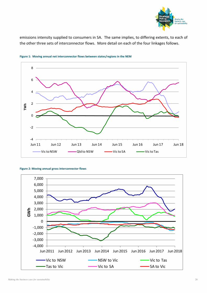
Making the business case for sustainability 28
emissions intensity supplied to consumers in SA. The same implies, to differing extents, to each of the other three sets of interconnector flows. More detail on each of the four linkages follows.
Figure 1: Moving annual net interconnector flows between states/regions in the NEM
Figure 2: Moving annual gross interconnector flows
-4
-2
0
2
4
6
8
Jun 11 Jun 12 Jun 13 Jun 14 Jun 15 Jun 16 Jun 17 Jun 18
TWh
Vic to NSW Qld to NSW Vic to SA Vic to Tas
-4,000-3,000-2,000-1,000
01,0002,0003,0004,0005,0006,0007,000
Jun 2011 Jun 2012 Jun 2013 Jun 2014 Jun 2015 Jun 2016 Jun 2017 Jun 2018
GWh
Vic to NSW NSW to Vic Vic to TasTas to Vic Vic to SA SA to Vic
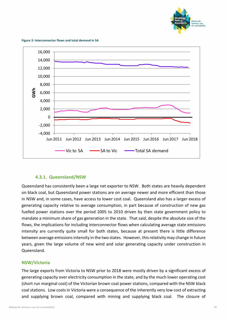
Making the business case for sustainability 29
Figure 3: Interconnector flows and total demand in SA
4.3.1. Queensland/NSW
Queensland has consistently been a large net exporter to NSW. Both states are heavily dependent on black coal, but Queensland power stations are on average newer and more efficient than those in NSW and, in some cases, have access to lower cost coal. Queensland also has a larger excess of generating capacity relative to average consumption, in part because of construction of new gas fuelled power stations over the period 2005 to 2010 driven by then state government policy to mandate a minimum share of gas generation in the state. That said, despite the absolute size of the flows, the implications for including interconnector flows when calculating average state emissions intensity are currently quite small for both states, because at present there is little difference between average emissions intensity in the two states. However, this relativity may change in future years, given the large volume of new wind and solar generating capacity under construction in Queensland.
NSW/Victoria
The large exports from Victoria to NSW prior to 2018 were mostly driven by a significant excess of generating capacity over electricity consumption in the state, and by the much lower operating cost (short run marginal cost) of the Victorian brown coal power stations, compared with the NSW black coal stations. Low costs in Victoria were a consequence of the inherently very low cost of extracting and supplying brown coal, compared with mining and supplying black coal. The closure of
-4,000
-2,000
0
2,000
4,000
6,000
8,000
10,000
12,000
14,000
16,000
Jun 2011 Jun 2012 Jun 2013 Jun 2014 Jun 2015 Jun 2016 Jun 2017 Jun 2018
GWh
Vic to SA SA to Vic Total SA demand
Making the business case for sustainability 30
Hazelwood power station in March 2017 brought supply capacity in Victoria into a much closer balance with state consumption. Over the past year, therefore, interconnector flows have mainly reflected market arbitrage opportunities, i.e. they are determined by variations in wholesale market prices between the two regions, which vary up and down over time in response to a variety of factors. Irrespective of the size of the net flows from Victoria to NSW, the much higher average emissions intensity of Victorian generation has obvious implications for the emissions intensity of electricity supplied to consumers in NSW, though these are currently less important than they were prior to this year.
4.3.2. Victoria/Tasmania
When the Basslink cable was built it was anticipated that electricity flows would be largely driven by arbitrage opportunities. Energy would be exported from flexible (fast response) hydro generators in Tasmania during peak demand times on the mainland, while at low demand times overnight Tasmania would import energy from inflexible (so-called baseload) brown coal generators in Victoria, allowing hydro storage levels to replenish. This is essentially the role envisaged for Tasmania under the “battery of the nation” proposal, and it has been a role which has been realised in practice. Over the years covered by Figures 1 and 2, however, that implied balance has been overridden by drought affecting energy availability in Tasmania and by commercially driven “over-generation” in Tasmania during the two year carbon price period, plus the cable outage lasting for six months from December 2015 to June 2016. Return to near balance means that on average electricity supplied to consumers in Tasmania includes some energy sourced from high emissions brown coal generators in Victoria, thereby increasing the average emissions intensity from the near zero level of the almost 100% hydro and wind generation in the state.
4.3.3. Victoria/SA
Until recently, SA was, like NSW, a large net importer of electricity from Victoria. As with NSW, this was largely driven by cost relativities; apart from a single, relatively high cost coal generator, which closed in 2016, SA depended on high cost gas generation, meaning that Victorian brown coal generators could almost always provide lower cost supply. However, the combination of the Hazelwood closure with the steadily growing supply of wind generation in SA has changed that balance. Victoria imports energy from SA when wind generation is at high levels and exports to SA during low wind periods, meaning that interconnector flows are now close to balance. However, the continuing flow of energy from Victoria to SA means that the average emissions intensity of electricity supplied to consumers in SA is higher than the emissions intensity of generation in the state.
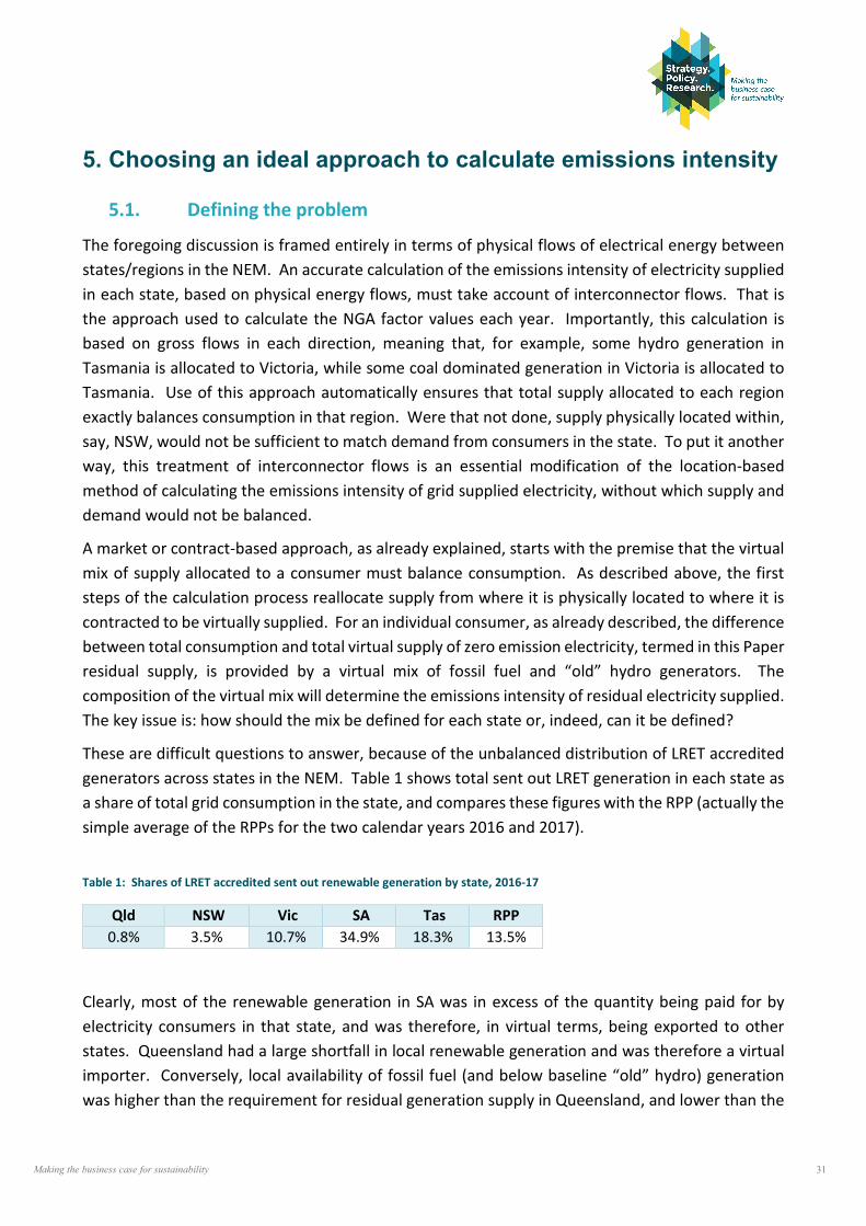
Making the business case for sustainability 31
5. Choosing an ideal approach to calculate emissions intensity
5.1. Defining the problem
The foregoing discussion is framed entirely in terms of physical flows of electrical energy between states/regions in the NEM. An accurate calculation of the emissions intensity of electricity supplied in each state, based on physical energy flows, must take account of interconnector flows. That is the approach used to calculate the NGA factor values each year. Importantly, this calculation is based on gross flows in each direction, meaning that, for example, some hydro generation in Tasmania is allocated to Victoria, while some coal dominated generation in Victoria is allocated to Tasmania. Use of this approach automatically ensures that total supply allocated to each region exactly balances consumption in that region. Were that not done, supply physically located within, say, NSW, would not be sufficient to match demand from consumers in the state. To put it another way, this treatment of interconnector flows is an essential modification of the location-based method of calculating the emissions intensity of grid supplied electricity, without which supply and demand would not be balanced.
A market or contract-based approach, as already explained, starts with the premise that the virtual mix of supply allocated to a consumer must balance consumption. As described above, the first steps of the calculation process reallocate supply from where it is physically located to where it is contracted to be virtually supplied. For an individual consumer, as already described, the difference between total consumption and total virtual supply of zero emission electricity, termed in this Paper residual supply, is provided by a virtual mix of fossil fuel and “old” hydro generators. The composition of the virtual mix will determine the emissions intensity of residual electricity supplied. The key issue is: how should the mix be defined for each state or, indeed, can it be defined?
These are difficult questions to answer, because of the unbalanced distribution of LRET accredited generators across states in the NEM. Table 1 shows total sent out LRET generation in each state as a share of total grid consumption in the state, and compares these figures with the RPP (actually the simple average of the RPPs for the two calendar years 2016 and 2017).
Table 1: Shares of LRET accredited sent out renewable generation by state, 2016-17
Qld NSW Vic SA Tas RPP 0.8% 3.5% 10.7% 34.9% 18.3% 13.5%
Clearly, most of the renewable generation in SA was in excess of the quantity being paid for by electricity consumers in that state, and was therefore, in virtual terms, being exported to other states. Queensland had a large shortfall in local renewable generation and was therefore a virtual importer. Conversely, local availability of fossil fuel (and below baseline “old” hydro) generation was higher than the requirement for residual generation supply in Queensland, and lower than the
Making the business case for sustainability 32
corresponding requirement in SA. In SA the shortfall in local residual supply was exacerbated by the fact that in 2016-17 it was a large (physical) net importer of electricity from Victoria.
As can be seen from the table, the other three states lie in a range between SA and Queensland. REC Registry figures suggest that WA also may have been a virtual net importer of LRET electricity. Note that it is not possible to be precise about any of these relativities because the total LGC requirement is not known on a state by state basis. This is because, according to advice from the Clean Energy Regulator, the distribution of EITE exempt consumption across states is commercially confidential and therefore not known, meaning that the volume of LRET liable retail sales in each state cannot be calculated.
In theory, the most obvious way to calculate the emissions intensity of residual supply would be to start by calculating the total requirement for residual supply in each state, following the series of steps shown in the flow diagram below – see Figure 4.
Unfortunately, the lack of state level data on EITE exemptions means that the first step cannot be undertaken. We explain here the nature and size of the calculation problems this presents, before examining possible second-best calculation options.
The size of these exemptions is material; nationally in 2017, including in WA, the NT and Mt. Isa, total relevant retail sales were 211.8 TWh. EITE exemptions for the same year totalled 40.2 TWh, i.e. about 20% of total relevant retail sales21. The referenced data show that aluminium smelting accounted for 62% of total exemptions. There are currently four aluminium smelters in Australia: one in Queensland and one in NSW, each of about equal capacity, a somewhat smaller one in Victoria, and a much smaller one in Tasmania22.. Based on the reported capacity and/or output of each, these smelters alone would reduce the “relevant acquisitions” of retail electricity by about 8.5 TWh in Queensland, 8.0 TWh in NSW, 5.5 TWh in Victoria, and 3.0 TWh in Tasmania. LGC requirements in each state in 2016-17 would be reduced by 13.5% of these amounts.
While currently small in volume, direct end user PPAs may also present data availability problems in future years. Current trends suggest that the volume of such contracts could grow quite rapidly. In principle, it may be possible to estimate the volume of electricity supplied through PPAs which combine the “black” (electrical energy) and “green” (LGS) components as the difference between total sent out generation from accredited wind and solar generators over a period and the number of LGCs generated over the same period. In practice, this number is likely to be quite small, at least for some time, meaning that errors and uncertainties related to either of the two large numbers may swamp the difference between them.
21 http://www.cleanenergyregulator.gov.au/DocumentAssets/Pages/Emissions-intensive-trade-exposed-activities-2017.aspx 22 https://aluminium.org.au/australian-industry/industry-description/australian-aluminium/
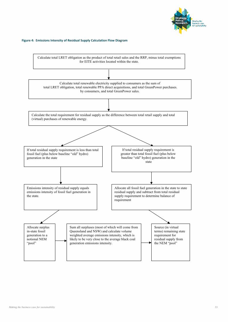
Making the business case for sustainability 33
Figure 4: Emissions Intensity of Residual Supply Calculation Flow Diagram
Calculate total LRET obligation as the product of total retail sales and the RRP, minus total exemptions for EITE activities located within the state.
Calculate total renewable electricity supplied to consumers as the sum of total LRET obligation, total renewable PPA direct acquisitions, and total GreenPower purchases.
by consumers, and total GreenPower sales.
Calculate the total requirement for residual supply as the difference between total retail supply and total (virtual) purchases of renewable energy.
If total residual supply requirement is greater than total fossil fuel (plus below baseline “old” hydro) generation in the
state
Allocate all fossil fuel generation in the state to state residual supply and subtract from total residual supply requirement to determine balance of requirement
Emissions intensity of residual supply equals emissions intensity of fossil fuel generation in the state.
Sum all surpluses (most of which will come from Queensland and NSW) and calculate volume weighted average emissions intensity, which is likely to be very close to the average black coal generation emissions intensity.
Source (in virtual terms) remaining state requirement for residual supply from the NEM “pool”
Allocate surplus in-state fossil generation to a notional NEM “pool”
If total residual supply requirement is less than total fossil fuel (plus below baseline “old” hydro) generation in the state
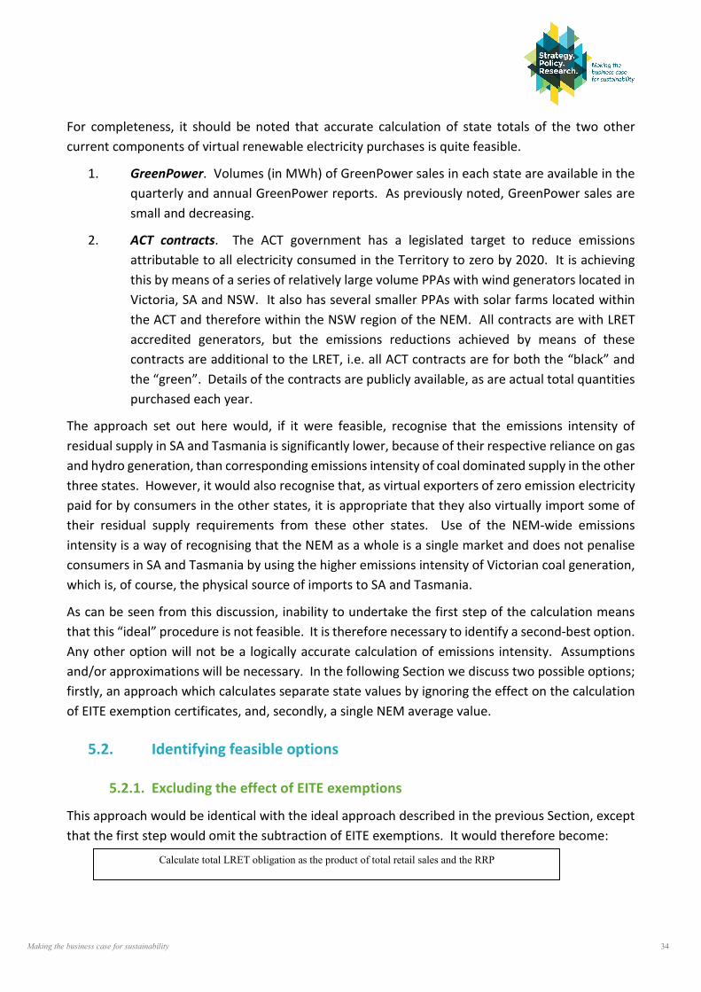
Making the business case for sustainability 34
For completeness, it should be noted that accurate calculation of state totals of the two other current components of virtual renewable electricity purchases is quite feasible.
1. GreenPower. Volumes (in MWh) of GreenPower sales in each state are available in the quarterly and annual GreenPower reports. As previously noted, GreenPower sales are small and decreasing.
2. ACT contracts. The ACT government has a legislated target to reduce emissions attributable to all electricity consumed in the Territory to zero by 2020. It is achieving this by means of a series of relatively large volume PPAs with wind generators located in Victoria, SA and NSW. It also has several smaller PPAs with solar farms located within the ACT and therefore within the NSW region of the NEM. All contracts are with LRET accredited generators, but the emissions reductions achieved by means of these contracts are additional to the LRET, i.e. all ACT contracts are for both the “black” and the “green”. Details of the contracts are publicly available, as are actual total quantities purchased each year.
The approach set out here would, if it were feasible, recognise that the emissions intensity of residual supply in SA and Tasmania is significantly lower, because of their respective reliance on gas and hydro generation, than corresponding emissions intensity of coal dominated supply in the other three states. However, it would also recognise that, as virtual exporters of zero emission electricity paid for by consumers in the other states, it is appropriate that they also virtually import some of their residual supply requirements from these other states. Use of the NEM-wide emissions intensity is a way of recognising that the NEM as a whole is a single market and does not penalise consumers in SA and Tasmania by using the higher emissions intensity of Victorian coal generation, which is, of course, the physical source of imports to SA and Tasmania.
As can be seen from this discussion, inability to undertake the first step of the calculation means that this “ideal” procedure is not feasible. It is therefore necessary to identify a second-best option. Any other option will not be a logically accurate calculation of emissions intensity. Assumptions and/or approximations will be necessary. In the following Section we discuss two possible options; firstly, an approach which calculates separate state values by ignoring the effect on the calculation of EITE exemption certificates, and, secondly, a single NEM average value.
5.2. Identifying feasible options
5.2.1. Excluding the effect of EITE exemptions
This approach would be identical with the ideal approach described in the previous Section, except that the first step would omit the subtraction of EITE exemptions. It would therefore become:
Calculate total LRET obligation as the product of total retail sales and the RRP
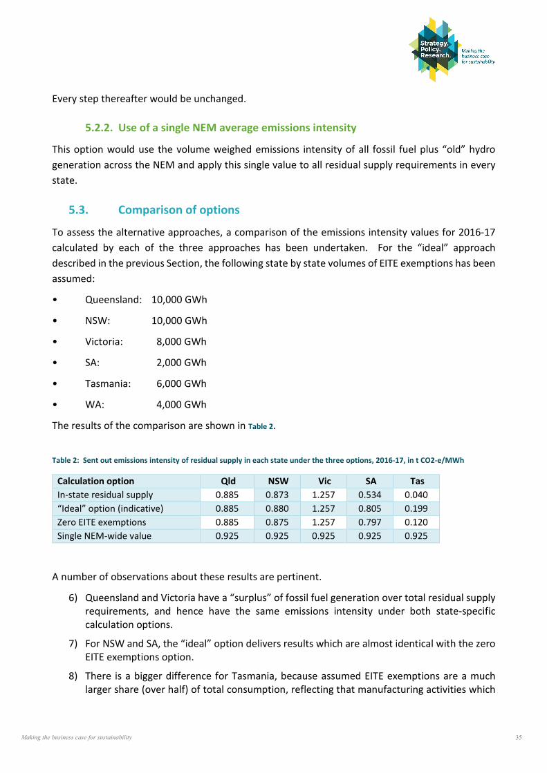
Making the business case for sustainability 35
Every step thereafter would be unchanged.
5.2.2. Use of a single NEM average emissions intensity
This option would use the volume weighed emissions intensity of all fossil fuel plus “old” hydro generation across the NEM and apply this single value to all residual supply requirements in every state.
5.3. Comparison of options
To assess the alternative approaches, a comparison of the emissions intensity values for 2016-17 calculated by each of the three approaches has been undertaken. For the “ideal” approach described in the previous Section, the following state by state volumes of EITE exemptions has been assumed:
• Queensland: 10,000 GWh
• NSW: 10,000 GWh
• Victoria: 8,000 GWh
• SA: 2,000 GWh
• Tasmania: 6,000 GWh
• WA: 4,000 GWh
The results of the comparison are shown in Table 2.
Table 2: Sent out emissions intensity of residual supply in each state under the three options, 2016-17, in t CO2-e/MWh
Calculation option Qld NSW Vic SA Tas In-state residual supply 0.885 0.873 1.257 0.534 0.040 “Ideal” option (indicative) 0.885 0.880 1.257 0.805 0.199 Zero EITE exemptions 0.885 0.875 1.257 0.797 0.120 Single NEM-wide value 0.925 0.925 0.925 0.925 0.925
A number of observations about these results are pertinent.
6) Queensland and Victoria have a “surplus” of fossil fuel generation over total residual supply requirements, and hence have the same emissions intensity under both state-specific calculation options.
7) For NSW and SA, the “ideal” option delivers results which are almost identical with the zero EITE exemptions option.
8) There is a bigger difference for Tasmania, because assumed EITE exemptions are a much larger share (over half) of total consumption, reflecting that manufacturing activities which
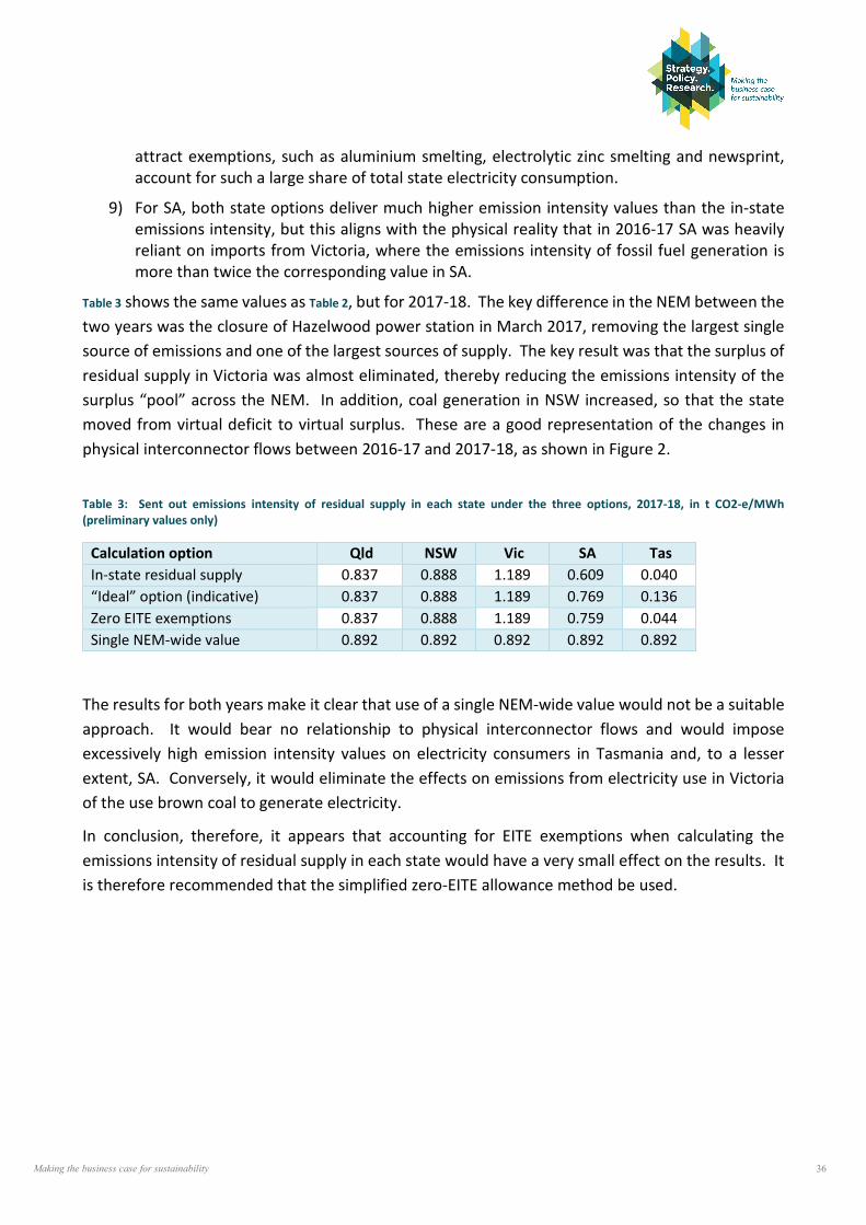
Making the business case for sustainability 36
attract exemptions, such as aluminium smelting, electrolytic zinc smelting and newsprint, account for such a large share of total state electricity consumption.
9) For SA, both state options deliver much higher emission intensity values than the in-state emissions intensity, but this aligns with the physical reality that in 2016-17 SA was heavily reliant on imports from Victoria, where the emissions intensity of fossil fuel generation is more than twice the corresponding value in SA.
Table 3 shows the same values as Table 2, but for 2017-18. The key difference in the NEM between the two years was the closure of Hazelwood power station in March 2017, removing the largest single source of emissions and one of the largest sources of supply. The key result was that the surplus of residual supply in Victoria was almost eliminated, thereby reducing the emissions intensity of the surplus “pool” across the NEM. In addition, coal generation in NSW increased, so that the state moved from virtual deficit to virtual surplus. These are a good representation of the changes in physical interconnector flows between 2016-17 and 2017-18, as shown in Figure 2.
Table 3: Sent out emissions intensity of residual supply in each state under the three options, 2017-18, in t CO2-e/MWh (preliminary values only)
Calculation option Qld NSW Vic SA Tas In-state residual supply 0.837 0.888 1.189 0.609 0.040 “Ideal” option (indicative) 0.837 0.888 1.189 0.769 0.136 Zero EITE exemptions 0.837 0.888 1.189 0.759 0.044 Single NEM-wide value 0.892 0.892 0.892 0.892 0.892
The results for both years make it clear that use of a single NEM-wide value would not be a suitable approach. It would bear no relationship to physical interconnector flows and would impose excessively high emission intensity values on electricity consumers in Tasmania and, to a lesser extent, SA. Conversely, it would eliminate the effects on emissions from electricity use in Victoria of the use brown coal to generate electricity.
In conclusion, therefore, it appears that accounting for EITE exemptions when calculating the emissions intensity of residual supply in each state would have a very small effect on the results. It is therefore recommended that the simplified zero-EITE allowance method be used.
Making the business case for sustainability 37
6. Other issues
6.1. Marginal Loss Factors
Marginal Loss Factors (MLFs) are prescribed by the NEM Rules as a means of allowing for energy losses in the transmission system when accounting for volumes of electricity supplied by a generator and received by a customer. As such, they are an essential component of the contractual settlement process in the National Electricity Market. Each year AEMO publishes a list of MLFs for all generators and all load connection points in each of the five NEM regions. There are a large number of different locations in each list. For example, the list of MLF values for 2018-19 for NSW includes 160 load locations (not including the ACT) and 51 supply locations.
In theory, MLFs could be applied to the calculations described above in two ways:
• they could be applied to generators to (in most cases) slightly reduce the volume of electricity they are effectively supplying to a load, meaning that more sent out generation would be required to deliver a specified quantity of electrical energy to a load, or
• they could be applied to a load to (in most cases) slightly increase the volume of sent out electricity required to supply the load.
However, adopting either approach would encounter a number of both conceptual and practical problems. AEMO has recently examined the effect of adjusting for MLFs in its calculation of the CDEII, by preparing what it calls Industry-Benchmark-Emission-Index (IBEI) values 23 . We have undertaken a systematic comparison of daily CDEII and IBEI values, as published by AEMO from the beginning of January to mid-June 2018. The outcome is that the daily IBEI values are higher than the corresponding CDEII values over that period by an average amount of 3.4% across the NEM as a whole, varying, depending on state/region, between a low of 2.0% in SA to a high of 4.8% in Victoria. We conclude that these differences are too small to justify the considerable additional complexity and labour required to use MLFs in the emissions calculations.
6.2. Inclusion of small rooftop solar
As previously noted, a small component of the cost of electricity for all electricity consumers (except those with EITE exemption) subsidises the installation of rooftop PV systems of a capacity less than 100 kW, through the workings of the Small Renewable Energy Scheme (SRES). That cost to consumer has not, however, been treated as a contract for the virtual supply of electricity, because
23 http://www.aemo.com.au/Electricity/National-Electricity-Market-NEM/Data/Settlements/Industry-Benchmark-Emission-Index
Making the business case for sustainability 38
the payment to rooftop PV owners is, in effect, a payment for capacity installed, not a payment for electricity supplied. The great majority of installations, especially household installations, supply some of the output to on-site consumption behind the meter and export the remainder into the local distribution network. Conceptually, the exported energy, at least, could be viewed as an additional source of renewable electrical energy to be accounted as part of the contracted zero emission electricity being supplied (in virtual terms) to all consumers. The case for doing so, however, is much less clear cut than it is for LRET generation. In the LRET case, the cost of LGCs represents the additional cost of making electricity “green”, relative to the basic wholesale price. Hence consumers are paying the whole cost of “greenness” (putting aside volatility in the cost resulting from the fact that LGCs are a market traded instrument). The same simple relationship between the SGC cost component of retail electricity prices and the cost of rooftop solar generation does not apply, because of the completely different structure of the cost of rooftop solar. There is no way of saying whether the SRES subsidy received by consumers who install rooftop solar is equal to, greater than, or less than the additional cost of the electricity supplied by rooftop solar. Hence, there is no way of saying whether the SRES component of retail prices is enough, less than enough, or more than enough to pay for a pro rata share the “greenness” of this electricity.
In addition, the practical and financial difficulties of including this electricity in the calculation of total emissions intensity would be almost insuperable. Most new rooftop solar installations now have the WiFi capability needed to transmit data to a relevant agency, but in a great many installations this capability is not enabled. Until a year or two ago, most installation did not even have the capability, so that a massive retrofit program would be required to even be able to collect the necessary data. Thus, while each individual rooftop solar owner knows precisely how much electricity the installation supplies in total, and how much of this total is exported, there are no aggregate totals for either at a state-wide level.
Several organisations, notably the Australian Photovoltaic Institute (APVI) and AEMO, make daily estimates of total generation, based on metered output from a sample of installations and total installed capacity. The two estimates usually vary by non-trivial margins, and these margins themselves also often vary, presumably because of differences in sample data and method, making it difficult to know which to prefer. The only comprehensive data on exports is that contained in the annual Regulatory Information Notice (RIN) responses, which each electricity network business submits to the Australian Energy Regulator (AER). The reporting template for electricity distribution businesses requires each business to report the volume of electrical energy received into the network from “residential embedded generation”. It is reasonable to assume that all, or almost all, of this energy is exports from rooftop solar systems. However, the same cannot be said for the corresponding energy received from “non-residential embedded generation”. This category will include some exports from smaller commercial rooftop solar (less than 100 kW), but it will also include exports from gas fuelled cogeneration installations. In addition, it will include exports from a wide variety of small-scale stand-alone generators, based on landfill gas, sewage gas, mini hydro, rooftop solar installations larger than 100 kW, and many other sources and technologies, all of which are LRET accredited and therefore already accounted for in the method we have proposed. The
Making the business case for sustainability 39
published data are not disaggregated by fuel or generation technology. Consequently, there is no complete source of data on exports from SRES accredited rooftop solar installations.
6.3. Diurnal and seasonal variations in the emissions intensity of electricity consumed
In Queensland, NSW and Victoria, the emissions intensity of electricity used overnight is usually higher than that of electricity used during the day and early evening. This has been the situation for many years, indeed, for decades, and is a manifestation of the inflexible technical and economic characteristics (frequently, and misleadingly, called baseload characteristics) of coal generation. This variation is of course a consequence of the normal shape of the diurnal load curve. The historical pattern was that larger, more modern coal generators were lower cost and therefore higher on the dispatch merit order. They ran for the full 24 hours, supplying what was called base load (note, a description of load, not of supply). As load increased during the day, higher cost, lower merit order coal generators increased output, but so too did lower emission gas and hydro generators. These general relationships remain today but have been given additional impetus by the rapid growth in small scale solar output, which is eroding the concept of baseload by often pushing the requirement for coal generation in the middle of the day to levels below the minimum overnight level. Since the start of 2018, the surge in new grid scale solar farm supply, particularly in NSW and Queensland, is exacerbating this effect.
Trading interval (30 minute) generation data provided by AEMO make it possible to calculate the average residual generation mix, following the procedures described in this Paper, in each of the 48 daily trading intervals over any period, such as a year. An electricity consumer would then be able to apply the resultant 30-minute emissions intensity to consumption during each of the three metering periods across a week (peak, shoulder and off-peak), or any other daily period for which comprehensive consumption data are available. Depending on its diurnal load shape, accurately reflecting differing emissions intensity during the three billing intervals could have quite a significant impact on a consumer’s total scope 2 emissions. On the other hand, this approach will obviously involve more analytical work than the default annual average approach we are proposing.
A separate, but also potentially important issue is that average daily emissions vary by season, because the mix of generation plant varies. We have undertaken a simple analysis of the seasonal effects in the NEM, starting in July 2014 (in order to avoid any effect of the short-lived price on emissions, which ended on 14 July 2014). Our proprietary model of NEM emissions has been used to calculate average NEM-wide emissions over this period in the four winter months, May to August, and the four summer months, December to March. Total electricity consumption in each of these eight months is consistently (in every year) higher than consumption in any of the remaining four months of each year.
Across the four-and-a-half-year period, the average emissions intensity of generation was consistently between 3 and 4 per cent higher in the summer months than in the winter months. Part way through the period, the closure of Hazelwood power station caused average NEM
Making the business case for sustainability 40
emissions intensity to fall by about 7 per cent, an effect increased somewhat by the fact that wind generation capacity grew steadily over the period, and so was higher after Hazelwood closed than before. These changes affected both summer and winter emissions, with the result that the average difference between summer and winter was much the same after the Hazelwood closure as before.
The main reason that emissions intensity is lower in winter, is that both hydro and wind generation are higher, on average, in winter than summer. However, more limited data on solar generation, covering the past two years only, show, as would be expected, that solar generation is significantly higher in summer than in winter. In future years, the more rapid growth of solar generation over the next few years can therefore be expected to moderate the difference in average NEM emissions intensity between winter and summer.
These calculations rely on the AEMO default set of average annual power station emission intensities, because the more accurate, recommended to be used for calculating annual emissions intensity, cannot be used for periods of less than one year.
Making the business case for sustainability 41
7. Conclusions and Next Steps This report notes that, at present in Australia, there are important risks associated unreconciled frameworks for accounting for greenhouse gas emissions associated with electricity consumption, and renewable energy consumption in particular. The risks include:
1. Non-recognition, in certain contexts, of the zero-carbon status of electricity consumption under PPAs, with potential detriment to those investing in PPAs
2. Double-counting of the emissions-benefits of renewable energy generation by different parties.
The report also highlights, however, that there is an opportunity to define, and populate with available data, a market-based methodology for greenhouse gas emissions associated with electricity consumption. This approach – which would complement and certainly not replace current regional-based accounting constructs – is consistent with international best practice as set out in the World Resources Institute’s GHG Protocol Scope 2 Guidance.
We expect that the market-based approach may be better suited than the alternative (and current default) approach of regional emissions-intensity factors to the increasing scale and complexity of renewable electricity generation and trade in Australia, at least in some circumstances.
It is timely to address these issues now, as there are expectations that the take-up of PPAs will only continue to grow in Australia in future, driven by market fundamentals such as the increasing cost-effectiveness of renewable electricity generation. PPAs can also offer terms and conditions that are attractive to at least some consumers, and which may enable them to better manage electricity price risks.
The methodology and available data sets explored here may not provide a complete response to the issues noted. However, they do provide a sound starting point and approach for addressing them. Ultimately, our aspiration is that this Report will assist governments and other parties to put in place effective arrangements to reduce the risks noted.

Contact
Philip Harrington
0419 106 449
Strategy. Policy. Research. Pty Ltd
ABN 38 615 039 864
www.strategypolicyresearch.com.au


