Calculation method based on CASMO/SIMULATE for …561359/FULLTEXT01.pdfCalculation method based on...

UPTEC-12027

Examensarbete 30 hpOktober 2012

Calculation method based on CASMO/SIMULATE for isotopic concentrations of fuel samples irradiated in Ringhals PWR

Tariq Zuwak

Teknisk- naturvetenskaplig fakultet UTH-enheten Besöksadress: Ångströmlaboratoriet Lägerhyddsvägen 1 Hus 4, Plan 0 Postadress: Box 536 751 21 Uppsala Telefon: 018 – 471 30 03 Telefax: 018 – 471 30 00 Hemsida: http://www.teknat.uu.se/student

Abstract

Calculation method based on CASMO/SIMULATE forisotopic concentrations of fuel samples irradiated inRinghals PWRTariq Zuwak

This is a M. Eng. degree project at Uppsala University carried out at Vattenfall NuclearFuel AB. The goal of it is to present a best estimate method based on the codepackage CASMO/SIMULATE for the purpose of calculating the isotopicconcentrations of a specified number of isotopes in a fuel sample. The calculationsdone with the method shall produce small deviations from reliable measured values,which characterize the accuracy of CASMO/SIMULATE, but also simplicity based onthe computing time and handling of the amount of data is an important factor in thedevelopment of the method.

The development of the method has been based on a sensitivity calculation withCASMO/SIMULATE on a number of relevant parameters affecting the isotopeconcentrations. The proposed method has then been applied on three samplesirradiated in Ringhals 4 and Ringhals 3. At last the calculated isotopic concentrationshave been benchmarked against measured data from Studsvik Laboratory.

The sensitivity analyzes has shown that the parameters affecting the neutronmoderation are very important for calculating the isotopic concentrations. The coreaxial resolution is also an important factor for the samples taken from top of the rod,where the power gradient is large. The comparison of the calculated and measuredvalues has shown that SIMULATE, in the analysed cases, simulates a lower finalburnup. This has created a need to correct the final burnup in order to get betterresults in terms of lower relative deviations between the measured and calculateddata.

Sponsor: Vattenfall Nuclear Fuel ABISSN: 1650-8300, UPTEC ES12027Examinator: Kjell PernestålÄmnesgranskare: Michael ÖsterlundHandledare: Klaes-Håkan Bejmer

1

Populärvetenskaplig sammanfattning Energiproduktion från kärnkraftsreaktorer följs idag med hjälp av mätningar och avancerade simuleringskoder. Exempel på parametrar som simuleras är effekt, neutronflödet i härden, utbränning av bränslestavar samt uppbyggnad av olika isotoper. För tryckvattenreaktorer använder Vattenfall kodpaketet CASMO/SIMULATE som är utvecklat av Studsvik Scandpower (SSP). Detta kodpaket förbättras kontinuerligt av SSP i syfte att öka nogrannheten och applikationerna. För att visa hur noga det verkliga förloppet simuleras kan koderna jämföras mot mätningar. Målet med detta arbete är att baserat på kod-‐paketet CASMO/SIMULATE ta fram en metod som på ett enkelt sätt kan beräkna halter av ett specifikt antal isotoper i ett bränsleprov. Metoden skall kunna användas för att verifiera beräkningsmodellen för isotopuppbyggnad i CASMO. Den skall ge ett bra resultat, d.v.s. beräkna olika isotoper vars avvikelser från tillförlitliga uppmätta värden är rimliga och karakteriserar beräkningsosäkerheten i CASMO/SIMULATE. Korta beräkningstider och enkelhet med tanke på hantering av mängden data är också viktiga faktorer i utvecklingen av metoden.

Utvecklingen av metoden har grundat sig på känslighetsanalyser av ett antal parametrar i CASMO/SIMULATE som påverkar isotopkoncentrationer. Metoden har sedan tillämpats på tre prover bestrålade i Ringhals 4 och Ringhals 3. Slutligen har de beräknade koncentrationerna jämförts med uppmätta värden från Studsvik laboratoriet.

Känslighetsanalyserna visade att de parametrar som påverkade neutron-‐modereringen är mycket viktiga för beräkningen av isotopkoncentrationer. Härdens axiella upplösning är av en stor betydelse för de prover som har tagits från toppen av staven, där effektgradienten är hög. Vid jämförelsen av de beräknade isotophalterna med de uppmätta värdena, har SIMULATE i samtliga fall simulerat en lägre slutlig utbränning. Detta har skapat behov av att korrigera den slutliga utbränningen och därmed få bättre resultat i form av lägre relativ avvikelse gentemot uppmätt data.

2

Executive summary The purpose of this project was to present a best estimate method based on the code package CASMO/SIMULATE for the purpose of calculating a specified number of isotopes in spent fuel sample. The method presented in this report calculates the isotopic concentration with reasonable deviations from measurements, which gives a reliable view of the amount of different isotopic concentrations in spent fuel. This may be useful to know for several purposes. One, and possibly even the most important purpose may be to use the appropriate materials for the final disposal of the spent fuel.

3

Table of Contents 1 Introduction ................................................................................................................. 4 1.1 Background ....................................................................................................................... 4 1.2 Goal ....................................................................................................................................... 4 1.3 Samples ............................................................................................................................... 5 1.3.1 Ringhals 4 PWR samples ....................................................................................................... 5 1.3.2 Ringhals 3 PWR samples ....................................................................................................... 6

1.4 Measurements .................................................................................................................. 7 1.4.1 Isotope Dilution Analysis ...................................................................................................... 7 1.4.2 Gamma Scan ............................................................................................................................... 8

1.5 Calculation tools .............................................................................................................. 9 1.5.1 SIMULATE ................................................................................................................................... 9 1.5.2 CASMO and CMSLINK ............................................................................................................. 9

2 Calculation method ................................................................................................. 10 2.1 SIMULATE ........................................................................................................................ 12 2.1.1 MATLAB .................................................................................................................................... 13

2.2 CASMO .............................................................................................................................. 13 2.3 CMPR ................................................................................................................................. 13 2.4 Correction of burnup ................................................................................................... 14 2.5 Sensitivity Analysis ...................................................................................................... 16 2.5.1 Number of depleted steps ................................................................................................. 17 2.5.2 Number of axial nodes ........................................................................................................ 17 2.5.3 Number of boron values ..................................................................................................... 17 2.5.4 Uranium enrichment ........................................................................................................... 17 2.5.5 Fuel temperature .................................................................................................................. 17 2.5.6 Uranium density .................................................................................................................... 17 2.5.7 Moderator density and inlet water temperature .................................................... 17 2.5.8 Water gap ................................................................................................................................. 18

3 Results ......................................................................................................................... 20 3.1 Sensitivity Analysis ...................................................................................................... 20 3.1.1 Group one ................................................................................................................................. 20 3.1.2 Group two ................................................................................................................................. 22 3.1.3 The best estimated method .............................................................................................. 26

3.2 Isotope concentrations of the assembly 50T and 3V5 ..................................... 27 3.2.1 Correction of burnup ........................................................................................................... 27 3.2.2 Comparison of the calculated and measured concentrations ............................ 27

4 Discussion .................................................................................................................. 32

5 Conclusions ................................................................................................................ 34 6 Acknowledgments ................................................................................................... 35

7 Bibliography .............................................................................................................. 36 Attachments ..................................................................................................................... 37 A. Isotope concentrations as function of burnup ...................................................... 37 B Calculation of burnup correction with Nd-‐isotopes ............................................. 47 C. Script ................................................................................................................................... 48

4

1 Introduction

1.1 Background The nuclear energy production is carefully followed in the operation by measurements and calculations. The power, neutron flux, burnup and the production of different isotopes in the fuel are simulated with advanced calculation codes during the whole fuel lifetime in the reactor. For this purpose Vattenfall uses different types of calculation codes. For the PWRs, the code package CASMO/SIMULATE (S3) supplied by Studsvik Scandpower (SSP) is used. This code package is continuously improved by SSP referring to accuracy and applications. In order to show the degree of improvement, the codes are benchmarked against other codes, but also against measurements. In this master of diploma work the calculation of burnup and isotopic concentrations are benchmarked against measured fuel samples. However, the calculation of isotope concentrations for a certain fuel rod is not straightforward. A lot of data must be calculated and used in the right way in order to get results with high accuracy.

1.2 Goal The goal is to present a best estimate method for comparisons of CASMO calculated vs measured isotopic concentrations. The development of the method shall be based on a sensitivity calculation with CASMO/SIMULATE on a number of relevant parameters affecting the isotope concentrations, see the project specification [1]. The calculations done with the method shall correctly calculate the isotopic concentration. The relative deviations from reliable measured values will characterize the uncertainty of CASMO/S3. But also the simplicity based on the computing time and handling of the amount of data is an important factor in the development of the method. The proposed method is applied on three samples irradiated in Ringhals 4 (R4) and Ringhals 3 (R3).

5

1.3 Samples

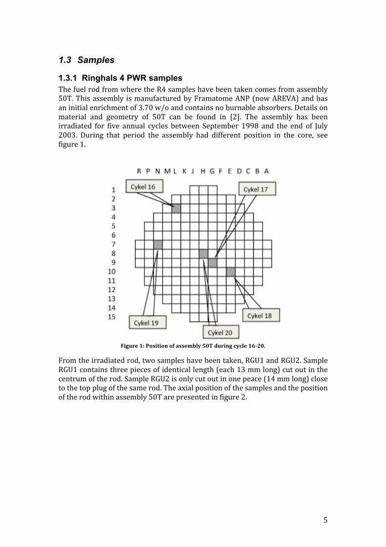
1.3.1 Ringhals 4 PWR samples The fuel rod from where the R4 samples have been taken comes from assembly 50T. This assembly is manufactured by Framatome ANP (now AREVA) and has an initial enrichment of 3.70 w/o and contains no burnable absorbers. Details on material and geometry of 50T can be found in [2]. The assembly has been irradiated for five annual cycles between September 1998 and the end of July 2003. During that period the assembly had different position in the core, see figure 1.

Figure 1: Position of assembly 50T during cycle 16-‐20.

From the irradiated rod, two samples have been taken, RGU1 and RGU2. Sample RGU1 contains three pieces of identical length (each 13 mm long) cut out in the centrum of the rod. Sample RGU2 is only cut out in one peace (14 mm long) close to the top plug of the same rod. The axial position of the samples and the position of the rod within assembly 50T are presented in figure 2.

6

Figure 2. The axial position of the sample and the position of the sample rod within assembly 50T.

1.3.2 Ringhals 3 PWR samples The isotope data for Ringhals 3 comes from the assembly 3V5. The sample rod was manufactured by Siemens (now AREVA) and operate for five annual cycles between July 2000 and May 2005 [3]. Figure 3 shows the position of the assembly 3V5 for each cycle.

Figure 3: Position of assembly 3V5 for each cycle.

The axial position and the position of the sample rod within assembly 3V5 are presented in figure 4.

7

Figure 4. The axial position of the sample and the position of the sample rod within assembly 3V5.

1.4 Measurements The isotope concentrations for these samples are experimentally determined at Studsvik Laboratory. The contents of the different isotopes are measured by different methods and some nuclides are analyzed with more than one method. Here are the methods, which have been used in the analysis [2]:

• Isotope Dilution Analysis (IDA) • Gamma Scan • ICP-‐MS Analysis with Separately Determined Response Factors • Analyses with external calibration • Residue Analysis

Only two of them are here below shortly presented, IDA and Gamma scan, since almost all the measured data come from these two methods. For details about the other methods, please, see [2].

1.4.1 Isotope Dilution Analysis The Isotope Dilution Analysis is used for most of the isotopes. This method is based on addition of a known amount of an enriched isotope, called "spike", to a sample. Isotopic ratios between the added isotope and the isotope to be analysed are determined by mass spectrometry. And then the amount of the isotope to be determined in the sample can be calculated according to following formula [2]:

NbS = Na

Sp ⋅

1− RMRSp

RM − R s

(1)

where

a = Spike isotope

8

b = Isotope to be analysed

Rs = Isotope ratio (a/b) in sample

RSp= Isotope ratio in spike

RM = Isotope ratio in mixture

NbS = Number of isotope b in sample

NaSp = Number of isotope a in spike

Once the isotope b has been determined, all other isotopes of the same element can be determined by the isotopic ratios measured by mass spectrometry.

The measured accuracy for the isotopes analyzed with the IDA is estimated to 1-‐5 %. However, the uncertainty for 142Ce is above 30 % for RGU1 and for 241Am and 243Am 25 and 22 %, respectively for RGU2.

1.4.2 Gamma Scan Axial gamma scanning was performed applying the technique of closely spaced point measurements. Instrument for the measurements, a high-‐purity germanium detector behind a 0.5 mm tungsten collimator was used. The detector and collimator system was adjusted to give photon energy independent activity values for a fuel rod with a certain diameter. The activities were decay corrected to the end of irradiation. A well-‐characterized reference rod segment (F3F6) was scanned together with the segments [2]. The main idea behind this method is to identify a number of correction factors in order to determine the absolute activity of the sample. The contributions of all these parameters are summarized in a general formula for determining of the absolute activity see equation 2.

dgEf

caa ⋅⋅⋅⋅=)(

1

γ

(2)

where a = Absolute activity [Bq/mm] a = Apparent (measured) activity [Bq/mm] f = Absorption factor Eγ = Energy peak g = Geometry factor d =Dead time correction factor

c= 137Cs reference rod correction c =aRR (tref )aRR (tref )

9

aRR =Activity of reference rod aRR= Apparent (measured) activity of reference rod tref = Time at end of irradiation of rod of concern For RGU1 and RGU2 the isotopes 103Ru, 106Ru, 134Cs, 137Cs and 154Eu have been analyzed with this method. All these isotopes have accuracy of about 5 %, except 154Eu, which has accuracy of about 20 %. Also, the prediction of the sample burnup was done using the gamma activity results for 137Cs. In addition to this gamma activity CASMO is used to determine the final burnup.

1.5 Calculation tools

1.5.1 SIMULATE SIMULATE (S3) is a three-‐dimensional calculation program used for both the PWR-‐ and BWR cores. In the calculation, the neutron flux are divided into high-‐energy flux (fast) and thermal flux, and the core is divided into a specific set of nodes. For example a fuel assembly is divided in 24 axial and four radial nodes, which means 96 nodes per fuel assembly. Simply, this means that SIMULATE solves a three-‐dimensional diffusion equation for the neutron flux at each node and connect the solutions between the different nodes with boundary conditions in order to describe the entire fuel core. Necessary input to SIMULATE is cross-‐sectional data describing the fuel design calculated by CASMO and is accessed through a linking program, CMSLINK. As further input to SIMULATE, core operating data as well as specification of the included fuel assemblies with their burnout histories can be mentioned.

1.5.2 CASMO and CMSLINK CASMO is a two-‐dimensional depletion transport theory code designed for fuel rods inside a fuel assembly. The idea behind this program is to place the fuel assembly in an infinite lattice in order to simulate the neutron transport inside and around the assembly. CASMO computes a multi-‐dimensional neutron flux distributions by solving the neutron transport eigenvalue problem. The solutions are used to compute different types of reactor physics’ parameters such as neutron flux, cross-‐sections, neutron age, buckling, isotope concentrations etc. CASMO contains a library of microscopic cross-‐section for a large number of nuclides. The input-‐data is given to CASMO via a file, which specifies lattice data (the fuel geometry, construction material, fuel enrichment and density), and boron level, power, fuel temperature, moderator density and temperature. The output consists of a large amount of data; the most important for this study is the isotope concentrations of the predefined nuclides. CMSLINK is a tool to convert the cross-‐sections from CASMO to a table used by SIMULATE.

10

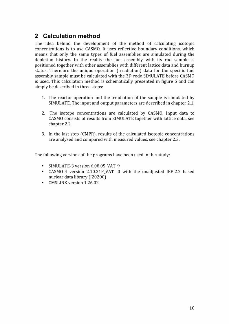
2 Calculation method The idea behind the development of the method of calculating isotopic concentrations is to use CASMO. It uses reflective boundary conditions, which means that only the same types of fuel assemblies are simulated during the depletion history. In the reality the fuel assembly with its rod sample is positioned together with other assemblies with different lattice data and burnup status. Therefore the unique operation (irradiation) data for the specific fuel assembly sample must be calculated with the 3D code SIMULATE before CASMO is used. This calculation method is schematically presented in figure 5 and can simply be described in three steps:

1. The reactor operation and the irradiation of the sample is simulated by SIMULATE. The input and output parameters are described in chapter 2.1.

2. The isotope concentrations are calculated by CASMO. Input data to CASMO consists of results from SIMULATE together with lattice data, see chapter 2.2.

3. In the last step (CMPR), results of the calculated isotopic concentrations are analysed and compared with measured values, see chapter 2.3.

The following versions of the programs have been used in this study:

• SIMULATE-‐3 version 6.08.05_VAT_9 • CASMO-‐4 version 2.10.21P_VAT -‐0 with the unadjusted JEF-‐2.2 based

nuclear data library (J20200) • CMSLINK version 1.26.02

11

Figure 5. Schematic view of the calculation method.

12

2.1 SIMULATE The simulation of the operation for the 5 cycles require a number of cycle specific input data as:

• Cycle length • Core operation power • Core loading pattern • Assembly burnup history data • Core cooling flux

The core follow operation and cooling flux values are measured by Ringhals with certain uncertainties, and consequently they can affect the calculation simulation of the core cycles. They are used as best estimated values and are not included in the sensitivity analysis of this study. Instead, the following input parameters are included in the sensitivity calculation, and hence the development of the isotopic concentration calculation method:

• Control rod bank position • Core inlet water temperature • Depletion steps • Number of axial nodes

Both the control rod bank position and core inlet water temperature are functions of the depletion. As more depletions steps are used, more different bank positions and temperatures must be given. The number of axial nodes affects the resolution of the results. A large number of axial nodes and depletions steps create a large number of data and long computing time. Simulation with S3 gives following output parameters:

• Nodal power density (3RPD) • Nodal fuel temperature (3TFU) • Nodal assembly exposure (3EXP) • Nodal density and reactor temperature of the moderator (3DEN and

TMO) • Nodal flux of both high-‐energy and thermal neutrons (3FLX, group 1 and

2)

13

2.1.1 MATLAB The output-‐file from SIMULATE contains a huge amount of data for all assemblies, at all nodes and for all parameters. MATLAB has been used for the purpose of reading the relevant parameters at the specific sample node for the specific assembly. The author has designed a script, exjobb_tz, used for this purpose. See Attachment C. Exjobb_tz is based on the script read_cms, which was first designed by Studsvik Scandpower. Read_cms reads the output-‐file from SIMULATE into Matlab. Exjobb_tz is divided into three parts.

• In the first part, the relevant parameters at the specific node for the specific assembly are read.

• In the second part boron values for each cycle are read and written. • In the last part an input-‐file including all the parameters necessary for

CASMO is generated.

2.2 CASMO When calculating the isotope concentrations with CASMO, all the output parameters (except nodal flux) from SIMULATE listed in chapter 2.1 are used as input, completed with:

• Initial lattice data (fuel enrichment, material and geometry) • Isotope specification

Using these parameters as input, CASMO calculates isotopic concentrations as function of nodal pin (sample) burnup.

2.3 CMPR Comparison of the calculated and measured concentrations has been done by calculating the relative deviation for each isotope, according to the following formula:

Re leative_ deviation = Calculated −MeasuredMeasured

(3)

The analysis is done in an excel-‐file, “Analysis-‐of-‐Isotope-‐concentrations.xls”.

14

2.4 Correction of burnup In order to make a fair comparison of the CASMO calculated and the measured isotopic concentrations, the concentrations must be compared at the same burnup level. There are a number of ways to do this correction.

One way is to use the fact that some isotopes are very well known to be both calculated and measured with high accuracy. For example the Neodymium (Nd) isotopes are often used in this type of studies. They are good burnup indicators also because of their weak neutron spectrum dependence and their none migration quality. By matching (linear regression) the calculated concentrations of the Nd-‐isotopes to their measured concentrations, the final burnup value can be corrected, see figure 6.

The 8 last calculated burnup values are presented in the figure with dots connected with a line. The measured values are presented with big dots at the final burnup value based on the 137Cs measured gamma profile.

Figure 6. Regression lines of the calculated concentrations and measured values

Every Nd-‐isotope contributes to the burnup value by its weight, which is dependent on the slope of its burnup dependence and the accuracy of the measurement of that isotope. The weight is proportional to the slope and inversed proportional to the measurement uncertainty. For example, the weight will be high for isotope curves with steep slopes and small measured uncertainties, for details see Attachment B.

15

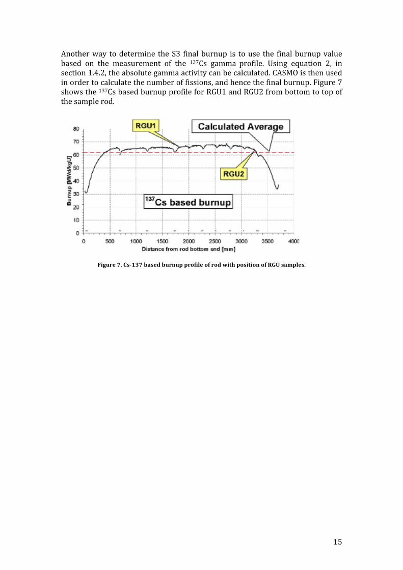
Another way to determine the S3 final burnup is to use the final burnup value based on the measurement of the 137Cs gamma profile. Using equation 2, in section 1.4.2, the absolute gamma activity can be calculated. CASMO is then used in order to calculate the number of fissions, and hence the final burnup. Figure 7 shows the 137Cs based burnup profile for RGU1 and RGU2 from bottom to top of the sample rod.

Figure 7. Cs-‐137 based burnup profile of rod with position of RGU samples.

16

2.5 Sensitivity Analysis As mentioned in section 2.1-‐2.3 a large number of parameters are input to both SIMULATE and CASMO. Each parameter has a different impact on the results. To find out how these parameters affect the isotopic concentrations and thus are important for the accuracy, a sensitivity analysis for some of the most important parameters is done, table 9.

Table 1. Sensitivity parameters

Parameters Reference Sensitivity

Number of depleted steps (NDS)

Best estimate Standard

Number of axial nodes (NAN)

12 24

Number of boron values (NBV)

1 value/depl.step 1 value/cycle

Uranium enrichment (UE)

Nominal +0,05 w/o (+1.4 %)

Fuel temperature (FT) 1 value/depl.step +50 K (+6 %)

Uranium density (UD) Nominal +0,1 g/cm3 (≈ +1%)

Moderator density (MD) 1 value/depl.step +0,05 g/cm3 (≈ +7%)

Inlet moderator temp. Best estimate +2 K

Water gap (WG) Nominal 0,01 cm (= +1,5 % volume water fuel ratio)

The sensitivity has been calculated by dividing the isotope concentrations for each case with the reference values, according to the following formula:

Sensitivity =[A]'−[A]ref[A]ref

(4)

Where

[A]'= Concentration of isotope A in the sensitivity case

[A]ref = Concentration of isotope A in the reference case

17

It should be noted that in this sensitivity study, no measured values are involved.

2.5.1 Number of depleted steps In order to carefully (with high resolution) follow the operation the number of depletion steps and operation data will be very high and hence the amount of data difficult to be handled. The aim of this calculation is to study the sensitivity on the results for a standard resolution compared to high resolution depletion steps. It is known that at the beginning and end of each cycle, the power gradient is high. This study investigates if more depletion steps, at the beginning and end of each cycle affect the results.

2.5.2 Number of axial nodes This part of the sensitivity analysis refers to core axial resolution. In the reference case, the core is divided into 12 axial nodes. In this part the sensitivity of changing the axial nodes to 24 is studied.

2.5.3 Number of boron values Usually, the boron depletion is simulated during the cycles. This means that a new boron value is used for each depletion step. In the sensitivity case only one average boron value is used for each cycle.

2.5.4 Uranium enrichment The suppliers deliver reliable fuel. However, there are still small uncertainties due to manufacturing reasons. The uncertainty in the 235U enrichment is typically less than 0.05 w/o. The initial enrichment level of the assembly 50T was 3.70 w/o with tolerance limit of ± 0.05 w/o. In this sensitivity case the enrichment level is increased to 3.75 w/o.

2.5.5 Fuel temperature Benchmarking of computer code predictions against measured fuel temperatures indicates that there is considerable uncertainty in calculated values. The resonance escape probability factor decreases with the fuel temperature, which in turn decreases the reactivity. However, the reactivity decrease will be partly compensated for by larger plutonium build up. In order to study how this phenomenon affects the isotope concentrations, a sensitivity analysis has been done for a 50 K higher fuel temperature.

2.5.6 Uranium density In this sensitivity case 0.1 g/cm3 higher uranium density than nominal has been studied. Besides the effect on the isotope concentrations, it is also interesting to compare the results with the corresponding results from the enrichment increase.

2.5.7 Moderator density and inlet water temperature The moderator density affects the neutron spectrum, which in turn affects the burnup and the build up of the different isotopes. The inlet water temperature, the water flux with its distribution inside the vessel, the control rod bank and the

18

power are the operation parameters, which are of great importance in the calculation of the local moderator density. Another source of error in order to predict the true moderator density is the calculation method itself with the interaction between S3 and CASMO. By comparing the neutron spectrum calculated by S3 and CASMO, this code interaction effect on the moderator density can be estimated. In this study two different calculations showing the sensitivity results for the uncertainties of the reactor operation parameters have been done. The first calculation aim to study the sensitivity results for the inlet water temperature, which is here increased by +2 K. The second calculation takes care of the rest of the input operation parameter uncertainties. The parameters affect each other in different degrees, which make the calculation difficult to perform. By assuming that the accumulated effect of the uncertainties of the input parameters affect the SIMULATE output of the moderator density with a certain value, the final effect of the CASMO isotopic concentration can be calculated. In this case, the accumulated value has been estimated to 0.05 g/cm3, which means about 7 % higher moderator density. This is however a very high density increase, which is based on the largest possible input error.

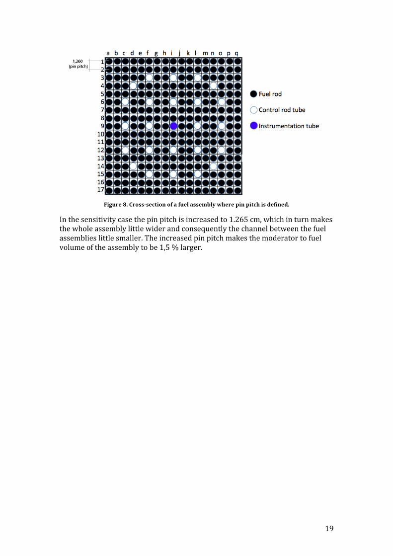
2.5.8 Water gap An important design parameter is the water gap between fuel assemblies. Experience from measurement of assemblies shows that the fuel assembly tends to be bend more or less. Both assembly bowing and rod bowing are well know, which means that the distance between the fuel rods in the assembly or the assemblies itselves are changed. This bowing phenomena gives rise to water gaps between rods and assemblies which deviate from nominal values. Figure 8 shows the cross-‐section of an ideal fuel assembly where the distance between two fuel rods is defined (pin pitch).

19

Figure 8. Cross-‐section of a fuel assembly where pin pitch is defined.

In the sensitivity case the pin pitch is increased to 1.265 cm, which in turn makes the whole assembly little wider and consequently the channel between the fuel assemblies little smaller. The increased pin pitch makes the moderator to fuel volume of the assembly to be 1,5 % larger.

20

3 Results

3.1 Sensitivity Analysis In order to clearly present the results, they are presented in two groups, with 5 and 4 sensitivity parameters in each group, respectively. The results are presented in figures 9-‐12 and in table 2 and 3.

3.1.1 Group one Group one consists of the following sensitivity parameters:

• Moderator density • Number of boron values • Number of depleted steps • Inlet temperature • Number of axial nodes

Figure 9. Sensitivity of number of depleted steps, axial nodes, boron values and moderator density for RGU1..

Figure 9 shows clearly that number of depleted steps, boron values, axial nodes and inlet water temperature have very low sensitivity for RGU1. The small inlet water temperature increase (0.8 %) affects the moderator density 0.5 % and hence affects the isotopic concentration very little. However, the second calculation with the 7 % higher moderator density affects the isotopic concentration very much, especially the actinides; 235U and 239Pu, which are the most important isotopes. The isotopes 235U and 239Pu have decreased by 11 % and 6 %, respectively. This is was also expected due to the exaggerated increase of the moderator density.

21

Figure 10. Sensitivity of the depleted steps, axial nodes, boron values and moderator density for

RGU2.

According to figure 10, the number of axial nodes has a larger impact on the results for the majority of the isotopes, especially for 235U, which has increased by over 10 %. The impact on 239Pu is, however, insignificant. The number of depleted steps and boron values and inlet water temperature has negligible impact on the results. Sensitivity of the moderator density is similar for RGU2 as RGU1. The isotopes 235U and 239Pu are decreased by 9 % and 7 % respectively.

22

3.1.2 Group two Group two contains the remaining parameters, which are:

• Uranium enrichment • Fuel temperature • Uranium density • Water gap

Figure 11. Sensitivity of uranium enrichment, fuel temperature, uranium density and water gap for

RGU1.

The sensitivity of uranium enrichment for RGU1 is relatively low for most of the isotopes including the actinides according to figure 11. Influence of this parameter is negligible for Pu isotopes and about 1 % for 235U. Fuel temperature has also a low sensitivity for majority of the isotopes, except 235U, which has sensitivity of about -‐1 %. The impact on Pu isotopes is less than 1 %. Uranium density and water gap are the parameters, which have largest sensitivity for most of the isotopes. Increasing uranium density and the volume ratio between moderator and fuel give less amount of 235U left, -‐3 % and -‐4 % respectively. For 239Pu the corresponding figures are +1.5 % and -‐1.0 % respectively.

23

Figure 12. Sensitivity of the uranium enrichment, uranium density, fuel temperature and water gap for RGU2.

Sensitivity of all the parameters for RGU2 shown in figure 12 looks almost the same as for RGU1. The uncertainty in uranium enrichment has a little influence on the fission products and the plutonium isotopes. The 235U left, is however, increased by about 3 %. Fuel temperature has a different sensitivity for RGU2 than for RGU1. For most of the isotopes the results are small negative values. However, the 235U has increased by 1 %. Notable parameters are still the uranium density and water gap. The 235U is decreased by 2 % and 3 % respectively. The239Pu is increased by 1 % and 0.25 %, for uranium density and water gap respectively. In table 2 and 3, all the sensitivity analyses of all parameters for different isotopes are presented for both RGU1 and RGU2. Total uncertainty is calculated for the parameters in group 2, by taking the square root of the quadratic sum of the parameters. All these parameters values without the fuel temperature contain uncertainties, which are impossible to avoid. Only the vendors of the fuel can minimize the tolerances by their own manufacturing process.

24

Table 2. Sensitivity analysis of group one parameter, RGU1.

GROUP 1 Group 2 Isotopes Number

of depleted steps

Number of axial nodes

Number of boron values

Inlet water temp.

Mod. dens.

Fuel temp.

Uran. dens.

Uran. enrich.

Water gap

Total uncertainty of group2

Mo95 -‐0,08% 0,04% -‐0,04% 0,44% -‐0,10% 0,36% 1,28% 0,71% 0,76% 1,80% Tc99 -‐0,08% 0,28% 0,01% 0,45% -‐0,13% 0,42% 1,14% 0,67% 0,62% 1,65% Ru101 -‐0,12% 0,32% -‐0,03% 0,52% -‐0,31% 0,42% 1,43% 0,56% 0,81% 1,95% Ru103 -‐1,15% 1,90% -‐0,97% 0,04% -‐1,15% 0,04% -‐0,18% -‐0,81% -‐0,40% 0,93% Ru106 0,14% 1,81% -‐0,79% 0,51% -‐1,31% 0,43% 1,04% -‐0,69% 0,34% 1,36% Rh103 -‐0,30% 0,11% -‐0,30% 0,40% -‐1,46% 0,50% 1,07% 0,40% 0,33% 1,29% Ag109 -‐0,29% 0,41% -‐0,14% 0,66% -‐0,59% 0,64% 1,91% 0,10% 1,05% 2,45% Cs133 -‐0,05% 0,25% 0,03% 0,43% 0,08% 0,43% 1,11% 0,68% 0,63% 1,62% Cs134 -‐0,12% 1,07% -‐0,72% 0,71% -‐3,04% 0,36% 2,21% -‐0,06% 0,79% 2,40% Cs135 0,07% -‐0,94% -‐0,37% 0,81% -‐3,90% 0,40% 1,90% 0,83% 0,00% 2,07% Cs137 -‐0,15% 0,32% -‐0,20% 0,51% -‐0,57% 0,39% 1,42% 0,43% 0,75% 1,80% La139 -‐0,15% 0,29% -‐0,05% 0,48% -‐0,45% 0,36% 1,44% 0,65% 0,80% 1,92% Ce140 -‐0,11% 0,31% 0,00% 0,53% -‐0,33% 0,39% 1,46% 0,68% 0,93% 2,04% Ce142 -‐0,14% 0,33% -‐0,04% 0,50% -‐0,44% 0,37% 1,43% 0,64% 0,80% 1,91% Ce144 0,65% 2,12% -‐0,96% 0,23% -‐1,31% 0,20% -‐0,24% -‐0,41% -‐0,51% 0,76% Pr141 -‐0,11% 0,24% -‐0,03% 0,50% -‐0,44% 0,38% 1,49% 0,67% 0,83% 1,99% Nd142 0,14% 0,58% 0,31% 1,03% 2,09% 0,64% 2,97% 0,72% 2,25% 4,27% Nd143 -‐0,62% -‐0,11% -‐0,69% 0,20% -‐4,17% 0,04% 0,63% 0,42% -‐0,38% 0,95% Nd144 0,01% 0,13% 0,41% 0,66% 1,66% 0,49% 1,97% 0,99% 1,59% 3,09% Nd145 -‐0,10% 0,24% -‐0,12% 0,41% -‐0,34% 0,36% 1,01% 0,71% 0,59% 1,51% Nd146 -‐0,24% 0,35% -‐0,14% 0,58% -‐0,53% 0,37% 1,65% 0,52% 1,01% 2,18% Nd148 -‐0,27% 0,37% -‐0,16% 0,53% -‐0,52% 0,39% 1,46% 0,56% 0,80% 1,95% Nd150 -‐0,29% 0,25% -‐0,21% 0,60% -‐0,82% 0,44% 1,63% 0,33% 0,91% 2,07% Pm147 0,11% 0,63% -‐0,30% 0,19% -‐0,10% 0,34% -‐0,14% 0,44% -‐0,24% 0,52% Sm147 -‐0,76% -‐1,31% 0,94% 0,36% 2,52% 0,67% 1,00% 1,74% 0,86% 2,59% Sm148 -‐0,29% -‐0,25% 0,03% 0,71% -‐1,32% 0,49% 2,21% 0,73% 1,00% 2,67% Sm150 -‐0,13% 0,50% -‐0,39% 0,47% -‐1,32% 0,32% 1,24% 0,29% 0,57% 1,47% Sm152 -‐0,11% 0,43% -‐0,17% 0,42% 0,89% 0,39% 0,85% 0,54% 0,71% 1,45% Sm154 -‐0,32% 0,53% -‐0,21% 0,72% -‐1,12% 0,62% 2,16% 0,16% 1,18% 2,69% Eu153 -‐0,10% 0,42% -‐0,04% 0,60% -‐0,63% 0,50% 1,67% 0,41% 0,93% 2,16% Eu154 -‐0,68% 0,16% -‐0,83% 0,51% -‐7,01% 0,44% 2,59% -‐0,58% -‐0,01% 2,66% Gd156 -‐0,24% 0,62% -‐0,03% 1,17% -‐0,05% 0,62% 3,53% 0,34% 2,32% 4,61% Gd158 -‐0,39% 1,06% -‐0,36% 1,15% -‐1,30% 0,66% 3,52% -‐0,11% 2,05% 4,44% U234 0,13% -‐0,30% 0,17% -‐0,39% 0,55% 0,00% -‐1,39% 1,68% -‐0,95% 2,45% U235 -‐1,58% -‐1,04% -‐1,79% -‐0,94% -‐11,16% -0,83% -‐3,30% 1,36% -‐4,30% 6,90% U236 -‐0,71% 0,05% -‐0,03% 0,26% -‐0,06% 0,09% -‐0,01% 1,56% -‐0,05% 1,56% U238 0,03% 0,03% 0,03% 0,06% 0,03% 0,03% 0,03% 0,03% 0,03% 0,06% Np237 -‐0,60% 0,16% -‐0,61% 0,42% -‐4,01% 0,36% 1,52% 0,74% 0,05% 1,69% Pu238 -‐1,37% -‐0,12% -‐0,91% 0,68% -‐6,38% 0,17% 3,01% 0,40% 0,78% 3,15% Pu239 -‐0,84% -‐0,17% -‐1,10% -‐0,09% -‐8,22% 0,35% 1,44% -‐0,80% -‐1,06% 2,10% Pu240 -‐0,97% -‐0,06% -‐0,61% 0,21% -‐2,49% -0,03% 0,62% -‐0,01% -‐0,04% 0,68% Pu241 -‐0,99% -‐0,15% -‐1,01% 0,19% -‐7,84% 0,38% 1,53% -‐0,78% -‐0,87% 2,02% Pu242 -‐0,10% 0,66% 0,03% 0,96% 1,02% 0,76% 2,32% 0,21% 1,80% 3,44% Am241 -‐1,66% -‐2,17% -‐1,22% -‐0,08% -‐10,08% 0,13% 1,80% 0,20% -‐0,81% 2,22% Am243 0,01% 0,73% -‐0,24% 1,20% -‐1,58% 1,31% 3,96% -‐0,22% 2,00% 4,99%

25

Table 3. Sensitivity analysis of all parameters for RGU2.

GROUP 1 GROUP 2 Isotopes Number

of depleted steps

Number of axial nodes

Number of boron values

Inlet water temp.

Mod. dens.

Fuel temp.

Uran. dens.

Uran. enrich.

Water gap

Total uncertainty of group 2

Mo95 -0,02% -2,82% -0,01% -0,15% -0,10% -0,15% 0,95% 0,72% 0,86% 1,65% Tc99 0,07% -2,78% -0,03% -0,12% -0,03% -0,12% 0,94% 0,61% 0,74% 1,52% Ru101 0,04% -3,53% -0,01% -0,13% -0,31% -0,13% 1,09% 0,55% 1,00% 1,81% Ru103 0,86% -5,60% -0,11% 0,07% -0,40% 0,07% 0,25% 0,20% 0,69% 1,16% Ru106 1,63% -6,89% 0,02% 0,01% -0,74% 0,01% 1,03% 0,11% 1,33% 2,16% Rh103 -0,09% -1,96% -0,05% -0,08% -1,15% -0,08% 0,98% 0,45% 0,53% 1,37% Ag109 0,00% -4,36% -0,06% -0,20% -0,63% -0,20% 1,51% 0,08% 1,28% 2,36% Cs133 0,06% -2,50% -0,04% -0,12% 0,07% -0,12% 0,83% 0,59% 0,71% 1,45% Cs134 0,96% -6,90% 0,18% 0,24% -2,42% 0,24% 1,91% 0,78% 1,85% 3,11% Cs135 -1,93% 0,73% 0,05% 0,27% -3,96% 0,27% 1,39% 1,09% 0,25% 1,79% Cs137 0,23% -3,71% 0,00% -0,12% -0,47% -0,12% 1,17% 0,61% 1,03% 1,90% La139 0,07% -3,28% 0,00% -0,11% -0,47% -0,11% 1,09% 0,67% 0,92% 1,76% Ce140 0,08% -3,50% 0,00% -0,03% -0,23% -0,03% 1,18% 0,75% 1,11% 2,03% Ce142 0,11% -3,49% 0,00% -0,03% -0,29% -0,03% 1,17% 0,75% 1,11% 2,03% Pr141 0,03% -3,21% 0,00% -0,12% -0,38% -0,12% 1,13% 0,66% 0,92% 1,83% Nd142 0,05% -7,41% 0,00% -0,30% 1,61% -0,30% 2,26% 0,44% 2,25% 3,71% Nd143 -0,14% -0,97% 0,06% 0,13% -3,28% 0,13% 0,60% 0,95% 0,24% 1,16% Nd144 -0,32% -4,09% -0,03% -0,29% 1,32% -0,29% 1,48% 0,59% 1,35% 2,37% Nd145 0,00% -2,57% -0,02% -0,11% -0,27% -0,11% 0,83% 0,69% 0,64% 1,43% Nd146 0,10% -4,18% 0,02% -0,13% -0,51% -0,13% 1,33% 0,65% 1,18% 2,12% Nd148 0,15% -3,71% 0,00% -0,12% -0,38% -0,12% 1,20% 0,59% 1,04% 1,96% Nd150 0,09% -3,97% 0,00% -0,11% -0,78% -0,11% 1,33% 0,49% 1,19% 2,12% Pm147 0,45% -1,20% -0,14% -0,14% 0,20% -0,14% -0,20% 0,58% -0,14% 0,64% Sm147 -2,13% 2,69% -0,14% -0,08% 1,70% -0,08% 0,78% 0,73% -0,14% 1,15% Sm148 -0,84% -3,34% 0,08% -0,01% -1,44% -0,01% 1,77% 0,73% 1,17% 2,46% Sm150 0,55% -4,12% 0,00% -0,09% -0,92% -0,09% 1,04% 0,60% 1,08% 1,85% Sm152 0,05% -3,00% -0,26% -0,34% 0,75% -0,34% 0,69% 0,41% 0,68% 1,24% Sm154 0,22% -5,13% 0,01% -0,13% -1,09% -0,13% 1,71% 0,28% 1,48% 2,66% Eu153 0,20% -4,07% 0,04% -0,10% -0,58% -0,10% 1,29% 0,44% 1,19% 2,10% Eu154 0,00% -4,18% 0,55% 0,69% -6,04% 0,69% 2,34% 0,76% 1,45% 3,13% Gd156 0,01% -8,32% 0,03% -0,36% -0,33% -0,36% 2,70% 0,24% 2,66% 4,27% Gd158 0,67% -8,97% 0,05% -0,18% -1,28% -0,18% 2,78% 0,21% 2,71% 4,44% U234 -0,18% 3,56% -0,04% 0,06% 0,62% 0,06% -1,05% 1,49% -1,16% 2,28% U235 -0,90% 10,21% 0,10% 0,88% -8,78% 0,88% -2,20% 2,56% -3,04% 5,19% U236 -0,86% -0,42% -0,07% 0,05% -0,06% 0,05% 0,02% 1,47% 0,00% 1,47% U238 0,00% 0,00% 0,00% 0,00% 0,00% 0,00% 0,00% 0,00% 0,00% 0,00% Np237 0,02% -3,03% 0,09% 0,25% -3,57% 0,25% 1,32% 1,22% 0,78% 2,07% Pu238 -0,57% -5,47% 0,23% 0,12% -5,72% 0,12% 2,59% 1,15% 1,92% 3,64% Pu239 0,12% 0,25% 0,37% 0,81% -7,34% 0,81% 1,39% 0,43% 0,25% 1,59% Pu240 -0,75% -1,73% -0,23% -0,02% -2,33% -0,02% 0,50% 0,18% 0,32% 0,62% Pu241 0,15% -1,28% 0,46% 0,63% -6,68% 0,63% 1,58% 0,52% 0,53% 1,91% Pu242 0,16% -6,31% -0,10% -0,30% 0,79% -0,30% 1,87% 0,00% 1,83% 3,16% Am241 -1,99% 3,97% 0,05% 0,40% -9,12% 0,40% 1,66% 0,78% -0,11% 1,84% Am243 0,70% -8,17% 0,11% -0,04% -1,55% -0,04% 3,33% -0,02% 2,63% 5,01% Cm244 0,94% -12,35% 0,16% 0,05% -3,96% 0,05% 4,89% -0,04% 4,10% 7,29% Cm245 1,36% -13,51% 0,82% 1,04% -11,26% 1,04% 6,52% 0,33% 4,78% 8,98%

26

3.1.3 The best estimated method It can be noticed from the sensitivity analysis that number of boron values and the depleted steps do not have remarkable effect on the results for both samples. Therefore it is enough accurate and simple to use the boron values and depletion data from the core follow standard calculation. Here simplicity and data handling have higher priority than calculation accuracy. The sensitivity analysis also shows that number of axial nodes has a significant influence on isotope concentrations for RGU2. Therefore In order to produce accurate results the method shall contain at least 24 axial nodes. It indicates that a high axial resolution is needed for samples close to the top and bottom nodes of the fuel. The sensitivity results of the moderator density indicate its large impact on the calculation of isotope concentrations. The input operation data to S3 affect that mostly, but also the way S3 and CASMO interact with each other might affect the results. By comparing the results of the neutron flux spectrum from the two codes, the calculation method can be studied. For all the 5 cycles the neutron flux ratio between fast and thermal neutrons from both S3 and CASMO were exactly the same, thereby confirming that the interaction between SIMULATE and CASMO for this aspect is excellent. One can conclude that the uncertainties coupled to moderator density are connected only to the input operation data and the calculation procedure in S3/CASMO codes themselves. Therefore, no correcting of the moderator density is needed and the best estimate values calculated by Simulate are good enough. Except fuel temperature, all the other parameters from group two are related to manufacturing with certain tolerance limits. There is a number of advanced fuel temperature codes, but all of them contain significant uncertainties. Benchmarking of theses codes against measured fuel temperature indicates that there is a considerable uncertainty in calculated values (about 100 K). It is nowadays difficult to find a code with uncertainty less than 50 K. For that reason the results of fuel temperature sensitivity analysis are included in the manufacturing product tolerances and a total impact of these uncertainties on the isotope concentrations are calculated. For 235U and 239Pu for RGU1 the total impact are 7 % and 2 %, respectively. The corresponding figures for RGU2 are 5 % and 2 %, respectively.

27

3.2 Isotope concentrations of the assembly 50T and 3V5

3.2.1 Correction of burnup For the correction of the final burnup, both methods described in section 2.4 have been studied. The method based on neodymium isotopes was first attempted, which for 50T-‐RGU1 and -‐RGU2 gave little higher burnup than S3 calculated, but lower than measured, based on gamma profile of 137Cs, as shown in table 4. For 3V5, the method of neodymium isotopes gave the lowest burnup compared to the other burnup values. Table 4. The S3 calculated, corrected and measured burnup.

S3 calculated burnup

The corrected burnup, based on Nd-‐isotopes

Measured burnup, based on gamma scan of 137Cs

Sample Assembly Sample Assembly Sample Sample

50T-‐RGU1 61.3 63.3 63.8 65.9 68 50T-‐RGU2 55.1 57.1 57.6 59.6 62 3V5 61.5 63.5 60 62 65 In this study the best agreement between the calculated and measured concentrations are achieved by adjusting the S3 final burnup value to the 137Cs gamma profile based value. All the comparison between measured and calculated isotope concentrations are presented before and after burnup correction, table 5-‐7.

3.2.2 Comparison of the calculated and measured concentrations The results in terms of relative deviation between the calculated and measured concentrations are presented in figure 13 and table 5, 6 and 7 for RGU1, RGU2 and 3V5 respectively.

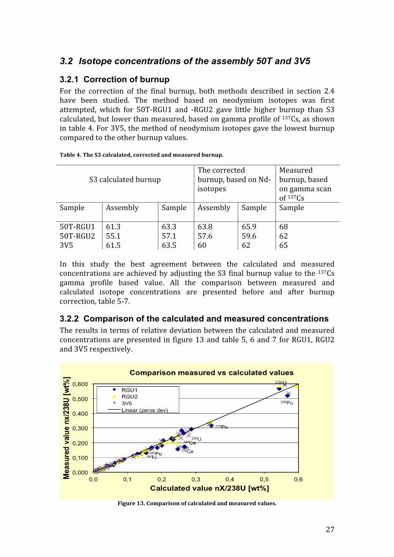
Figure 13. Comparison of calculated and measured values.

28

Figure 13 aims to show the agreement between the results from measurements and calculation, but also identify the points positioned far outside the “zero deviation” line for all three cases. The points with high values far from the line, here defined as outlayers, are clearly seen in this type of plot. The out layers are 99Tc, 239Pu, 240Pu, 242Pu and 142Ce for RGU1, 236U and 140Ce for RGU2 and 140Ce, 235U, 236U, 239Pu and 240Pu for 3V5. The relative deviation between calculated and measured values is shown in table 5,6 and 7. For the absolute values, please see attachment D. It can be noticed that for some fission products the deviation between calculated and measured values increases after burnup correction. However, the most important nuclides, which are the actinides, generally give best results after burnup correction. For 235U, the deviation before the correction was 31.3 %, 24.8 % and 21.8 %, which decreased to -‐0.5 %, -‐1.7 % and 5.5 % for RGU1, RGU2 and 3V5 respectively. For 239Pu, the deviation before the correction was 12.0 %, 3.6 % and 7.5 %, which decreased to 9.3 %, 2.0 % and 2.5 % for RGU1, RGU2 and 3V5 respectively. Most of the fission product isotopes have been improved after burnup correction in the three cases. The relative deviations of the isotopes 140Ce and 142Ce for RGU1, after burnup correction, are 54 % and 57 %, which are quite unreasonable. The corresponding values for RGU2 are 20.1% and 10.9 % and for 3V5 10.2 and 2.9 %, respectively. The burnup correction has resulted in a higher relative deviation for the isotopes 147Pm, 152Sm, 153Eu, 154Eu, 158Gd, 234U, 244Cm and 245Cm. Common for these isotopes is that they are in small quantities and in some cases combined with a larger uncertainty in measured data. However, it can be mentioned that 18 of 42 isotopes has resulted in a lower relative deviation for RGU1. The corresponding values for RGU2 and 3V5 are 23 of 42 and 18 of 34 isotopes, respectively. The isotopic concentrations as function of burnup at the end of the cycle are shown in attachment A for all three cases. It can be mentioned that some isotopes are more or less dependent on the burnup, depending on how steep the slope of the curve is. The steeper the slope curve has, the stronger the dependence and vice versa. The 235U is strongly dependent on burnup while 234U, which is almost constant and not affected at all.

29

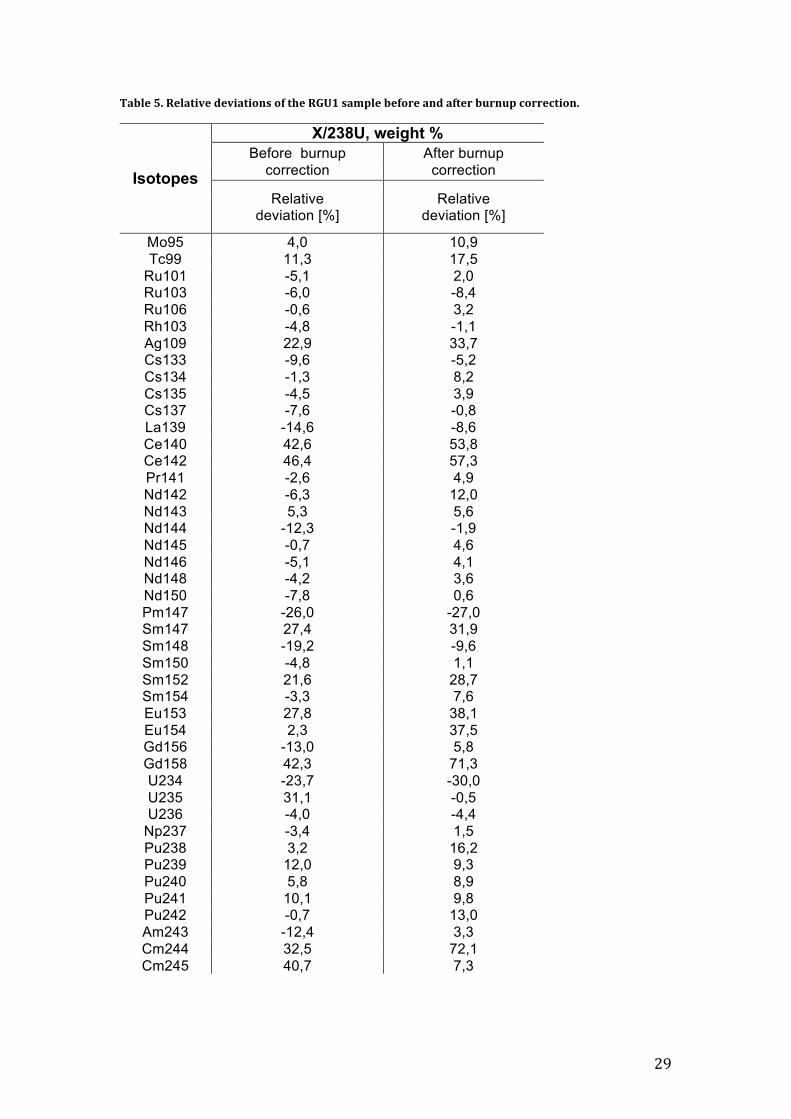
Table 5. Relative deviations of the RGU1 sample before and after burnup correction.

Isotopes

X/238U, weight % Before burnup

correction After burnup

correction

Relative deviation [%]

Relative deviation [%]

Mo95 4,0 10,9 Tc99 11,3 17,5

Ru101 -5,1 2,0 Ru103 -6,0 -8,4 Ru106 -0,6 3,2 Rh103 -4,8 -1,1 Ag109 22,9 33,7 Cs133 -9,6 -5,2 Cs134 -1,3 8,2 Cs135 -4,5 3,9 Cs137 -7,6 -0,8 La139 -14,6 -8,6 Ce140 42,6 53,8 Ce142 46,4 57,3 Pr141 -2,6 4,9 Nd142 -6,3 12,0 Nd143 5,3 5,6 Nd144 -12,3 -1,9 Nd145 -0,7 4,6 Nd146 -5,1 4,1 Nd148 -4,2 3,6 Nd150 -7,8 0,6 Pm147 -26,0 -27,0 Sm147 27,4 31,9 Sm148 -19,2 -9,6 Sm150 -4,8 1,1 Sm152 21,6 28,7 Sm154 -3,3 7,6 Eu153 27,8 38,1 Eu154 2,3 37,5 Gd156 -13,0 5,8 Gd158 42,3 71,3 U234 -23,7 -30,0 U235 31,1 -0,5 U236 -4,0 -4,4

Np237 -3,4 1,5 Pu238 3,2 16,2 Pu239 12,0 9,3 Pu240 5,8 8,9 Pu241 10,1 9,8 Pu242 -0,7 13,0 Am243 -12,4 3,3 Cm244 32,5 72,1 Cm245 40,7 7,3

30

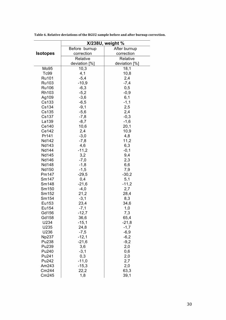
Table 6. Relative deviations of the RGU2 sample before and after burnup correction.

Isotopes

X/238U, weight % Before burnup


correction Relative

deviation [%] Relative

deviation [%] Mo95 10,3 18,1 Tc99 4,1 10,8

Ru101 -5,4 2,4 Ru103 -10,9 -7,4 Ru106 -6,3 0,5 Rh103 -5,2 -0,9 Ag109 -3,6 6,1 Cs133 -6,5 -1,1 Cs134 -9,1 2,5 Cs135 -5,6 2,4 Cs137 -7,8 -0,3 La139 -8,7 -1,6 Ce140 10,6 20,1 Ce142 2,4 10,9 Pr141 -3,0 4,8 Nd142 -7,8 11,2 Nd143 4,6 6,3 Nd144 -11,2 -0,1 Nd145 3,2 9,4 Nd146 -7,0 2,3 Nd148 -1,8 6,6 Nd150 -1,5 7,9 Pm147 -29,5 -30,2 Sm147 0,4 5,1 Sm148 -21,6 -11,2 Sm150 -4,0 2,7 Sm152 21,2 28,4 Sm154 -3,1 8,3 Eu153 23,4 34,6 Eu154 -7,1 1,0 Gd156 -12,7 7,3 Gd158 36,6 65,4 U234 -15,1 -21,8 U235 24,8 -1,7 U236 -7,5 -6,9

Np237 -12,1 -6,2 Pu238 -21,6 -9,2 Pu239 3,6 2,0 Pu240 -3,1 0,6 Pu241 0,3 2,0 Pu242 -11,0 2,7 Am243 -15,3 2,0 Cm244 22,2 63,3 Cm245 1,8 39,1

31

Table 7. Relative deviation of the 3V5 sample before and after burnup correction.

Isotopes

Calculations, X/238U, weight % Before burnup


correction

Deviation [%] Deviation [%]

Cs133 -7,7 -6,1 Cs134 26,1 25,9 Cs135 -8,6 -5,0 Cs137 -5,7 -3,7 La139 -4,2 -2,0 Ce140 7,1 10,2 Ce142 0,6 2,9 Nd142 1,3 7,4 Nd143 10,6 11,6 Nd144 -4,1 0,6 Nd145 6,3 8,1 Nd146 0,7 3,7 Nd148 0,2 2,6 Nd150 2,2 5,1 Sm147 -10,8 -6,1 Sm148 -16,1 -12,4 Sm150 -1,1 0,6 Sm152 20,9 23,3 Sm154 1,6 5,0 Eu153 32,8 36,4 Eu154 73,4 75,6 Gd156 3,6 11,8 Gd158 59,9 68,7 U234 -15,3 -17,2 U235 21,8 5,5 U236 -5,0 -5,0

Np237 -4,6 -2,5 Pu238 -9,0 -4,1 Pu239 7,5 2,5 Pu240 2,6 0,6 Pu241 10,0 9,0 Pu242 1,3 5,7 Am241 -35,3 -27,0 Am243 -15,0 1,7

32

4 Discussion The fresh nuclear fuel consists only of the uranium isotopes. The actinides, Pu Cm, Np and Am, as well as the fission products are produced during the operation. The neptunium isotopes and 238Pu originate from neutron capturing of 235U while the other actinides are a result of neutron capturing of 238U. The isotopes 235U, 239Pu and 241Pu make the major contribution to the energy release and maintenance of the chain reaction. Some actinides, which are build-‐up faster than they decay, will increase along with burnup. Other isotopes, which are created as fast as they decay, achieve a balance and will remain constant along with burnup. However, 235U, which makes the major contribution to the energy release and is not build-‐up during the operation, will obviously decrease along with burnup. This means that the final burnup of a fuel is an important parameter for the concentrations of the isotopes highly influenced by burnup, for example 235U, 144Nd, 150Sm, 237Np, 152Sm and 137Cs. It is also confirmed by the burnup correction giving better results for these types of isotopes, except the isotopes 140Ce and 142Ce, which have a positive gradient along with burnup and the measured value is much lower than calculated for both RGU1 and RGU2. In this case, the measured concentrations of these isotopes must be uncertain. The other isotopes giving worse results after burnup correction are usually in small amounts and combined with greater uncertainties. Increasing the uranium enrichment in the sensitivity analyzes, was a good example of a parameter affecting the final burnup. An increase in uranium enrichment means increasing the fissile nuclei, 235U. Since there are increasing number of 235U, it means there should be relatively more 235U left at the end of the cycle, as demonstrated by sensitivity analysis. For RGU1 the increase of 235U was about 1 % and the corresponding value for RGU2 was almost 3 %. The 239Pu was decreased by about 1 % for RGU1 and for RGU2 the isotope was increased by 0.4 %. This may be due to better moderating at the position of RGU1, which caused more fission of 235U and less build up of 239Pu. At position of RGU2, the moderator density is lower, which means that the neutron spectrum is harder and consequently the more 239Pu are built up. Another phenomenon affecting the isotopic concentrations is the neutron spectrum in the core. The neutron spectrum affects not only the build up of plutonium but also the distribution of the fissions products from 235U and 239Pu. This will affect the isotopic concentrations because these isotopes have slightly different fission product yields, and hence tendency to form some isotopes more than others. This is the second main phenomenon that affects the isotopic concentration and appears in some of the sensitivity analyzes. Moderator density is a good example of the parameter causing a change in the neutron spectrum. For the RGU1 sample the isotopes 235U and 239Pu has decreased by 11 % and 6 % due to higher value of the moderator density. A higher moderator density means that more neutrons are slowed down to

33

thermal energy, which in turn increases the fissions of 235U and decreases the build up of 239Pu. This explains the decrease of 235U and 239Pu concentrations. Furthermore, it should also be noted that in this sensitivity analysis the moderator density was changed by +0.05 g/cm3, which is a high perturbation. It may be compared with the sensitivity analysis of inlet water temperature, which was changed only by 2 degrees resulting in a change in moderator density of only -‐0.004 g/cm3. Even that little change could affect 235U about -‐1 % and +1 % for RGU1 and RGU2 respectively. Increasing the pin pitch 0.01 cm made the moderator to fuel volume ratio 1.5 % larger. This is another example on the parameter causing a change in the neutron spectrum. A higher moderator to fuel volume ratio increases the resonance passage factor (p) because of increasing the probability for the neutron to be slowed down to thermal energy before being captured in 238U. On the other hand, the thermal utilization factor (f) is decreased by a larger volume ratio of moderator and fuel, because of increasing probability for the neutron capture in the moderator. Since these two parameters are included in the four-‐factor formula, the product of these parameters gives the optima. For PWR reactors, which are in general undermoderated an increased moderator to fuel volume ratio means an increased reactivity level. The results from this analysis show a decrease of 4 % and 3 % of 235U for RGU1 and RGU2 respectively, indicating on a softer neutron spectrum and less 239Pu buildup. The sensitivity analyses of the depletion steps showed not much impact on the isotopic concentrations. This is because SIMULATE follows the operation curve well enough, which means that there is no need for additional depletion steps. The number of axial nodes was an important parameter for the samples taken from top and bottom of the rod where the power gradient is large. A large number of axial nodes means a better resolution that gives more accurate information about the core. The RGU2 sample that was taken from a quite high level of the rod is an excellent example showing a high sensitivity for 235U, which was 11 %. The corresponding value for RGU1 sample, where the power is quite constant, was -‐1 %. The sensitivity analysis of boron values has shown no remarkable impact on isotopic concentrations. This is because the average boron values remains the same for all five cycles, hence there is no change in the neutron spectra.

34

5 Conclusions Benchmarking the calculated data against measured is not that easy since there are a lot of parameters inducing uncertainties. The uncertainties could be involved at the measured data as well as the calculated, which makes it difficult to point out what is wrong. But calculation of the relative deviation is still a good indicator. Based on this, the following conclusions are drawn:

• The results of the comparison between measured and calculated isotopic concentrations show good agreement on the most important isotopes, which indicates that the calculation method (CASMO/S3) is accurate. For example 235U and 239Pu.

• The isotopes with small measured amount and with small burnup

dependence show large deviation. For example 241Am, 152Sm, 153Eu, 244Cm and 158Gd.

• The core axial resolution is very important parameters for a sample taken

from top or bottom of the rod, where the power gradient is large.

• The accuracy of the results is very much dependent on correct sample burnup and correct simulation of the neutron spectrum. A larg part of these uncertainties have their origin in the input parameters of the calculation method. The combined impact of tolerances for fuel temperature, enrichment, uranium density and standard rod/assembly bowing are for 235U and 239Pu 5-‐7 % and 2 % respectively.

• The calculation procedure for isotopic comparisons is fast and more or

less automatic. SIMULATE runs the reactor simulation, CASMO calculates the different isotope concentrations and CMPR analyses the data and make table and figures. The data between the different programs are easily handled by scripts in MATLAB.

• The goal of the project has been achieved by presenting a best estimate

method for comparisons of CASMO calculated vs measured isotopic concentrations. The calculations done with the method calculates the isotopic concentration correctly and the relative deviations from reliable measured values characterize the uncertainty of CASMO/S3.

35

6 Acknowledgments I would like to express my most sincere thanks to my supervisor at Vattenfall Nuclear Fuel AB, Klaes-‐Håkan Bejmer. He has assisted me throughout the entire project and given me lots of good advices. I have always felt welcome to him with any question and he has answered in a very friendly manner, which is something I have really appreciated. I can also not forget some professional advices I have received from Ewa Kurcyusz-‐Ohlofsson at Vattenfall Nuclear Fuel AB. Her advices have been very crucial in some situations. Furthermore I want to thank Thomas Smed at Studsvik Scandpower who has helped me with loading files into MATLAB. My script is based on some functions in his script, which has been of crucial importance to the execution of the project. Hans-‐Urs Zwicky and Michael Granfors at Studsvik invited my supervisor and I to the Studsvik Laboratory, where they described the methods of measurements and I am very grateful for their contribution to this project.

36

7 Bibliography

1. Tariq, Z. (2012). Project specification. Stockholm.

2. Zwicky, H.-‐U., Low, J., & Granfors, M. (2011). MALIBU Extension Nuclide Analyses Performed at Studsvik. Studsvik.

3. Zwicky, H.-‐U., Low, J., & Ekeroth, E. (March 2011). Corrosion Studies with

High Burnup Ligher Water Reactor Fuel. Studsvik: Studsvik Nuclear AB.

37

Attachments

A. Isotope concentrations as function of burnup

38

39

40

41

42

43

44

45

46

47

B Calculation of burnup correction with Nd-isotopes Assume that the adjusted burnup value, Xm (matching value), has small impact on the calculated shape of the isotopic concentration curve (as a function of burnup). Use only those isotopes, which are, based on experience, easy to calculate and measure with high accuracy. The burnup for a certain isotope, Xi, can be given as a function of the calculated concentration and the shape. Instead of the calculated concentration, use the measured one, Yi. The new burnup value, Xmi is then;

Xmi = Xmi(Yi,Si) and X1mi = X1mi((Yi+Di),Si) (determined with regression analysis) Where;

• Yi = the measured value for the matching isotope i, D is the measured accuracy for that isotope.

• Si = the calculated shape, which for a line is characterized by the slope and

a constant. The slope is inverse proportional to the burnup and the constant is proportional.

The weight for this isotope can then be calculated as; Wi = 1/(X1mi-‐Xmi) The adjusted burnup is calculated as; Xm = Si (Xmi*Wi)/S Wi

48

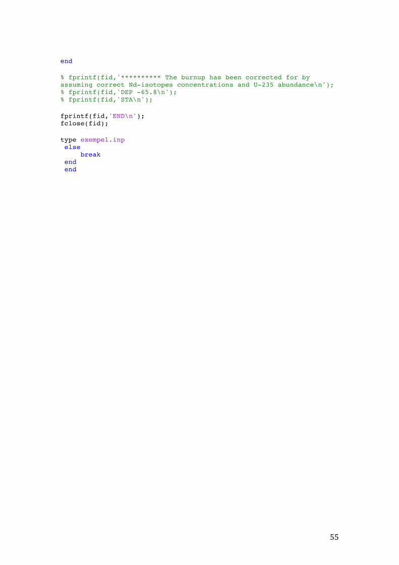
C. Script %% Denna script anv√§nds f√∂r att l√§sa ut n√•gra f√∂rutvalda parametrar i en specifik nod %% och i x antal cyklar, fr√•n en cms-fil. % Scripten best√•r av 3 delar, uppdelade i 3 kapitel. % Del 1 h√§mtar data fr√•n en cms fil och visar slutresultat enligt tidigare beskrivning i matrisen 'Resultat'. %Del 2 h√§mtar borv√§rdena och utbr√§nningar fr√•n en csv-fil och ritar en regressionslinje s√• att man kan %ber√§kna borv√§rde utifr√•n ett valfritt v√§rde p√• utbr√§nning. %Del 3 skriver ut n√•gra av de tidigare parametrarna och f√∂rbereder en textfil %som sedan ska k√∂ras i CASMO. %% 1.1 Hittar r√§tt mapp till filen och l√§gger till path-filerna som √§r n√∂dv√§ndiga f√∂r att kunna anropa CMSREAD-metoden clear all clc cd /home/pwr/Projekt/Isotopber-2011/Exjobb-2012/sim3/ % hitta r√§tt mapp till filen %al√§gg till path-filerna addpath /home/user/tzuw/Mfiler addpath /home/prog/dvlp/CMSCODES/CMSlab/S3kPlot addpath /home/prog/dvlp/CMSCODES/CMSlab/cmsview addpath /home/prog/dvlp/CMSCODES/CMSlab/CmsTools addpath /home/prog/dvlp/CMSCODES/CMSlab/CmsPlot addpath /home/prog/dvlp/CMSCODES/CMSlab/cmscore addpath /home/prog/dvlp/CMSCODES/CMSlab/CmsRead cmsinfo=read_cms('simout_50T_16-20.cms'); mat=[]; %skapa en tom matris som senare fylls i m.h.a for-loopen nedan: %% 1.2 Metod f√∂r att k√§nna av antalet utbr√§nningssteg och l√§ngden av respektive cykel utbsteg= read_cms_scalar(cmsinfo,'CYCLE EXPOSURE (GWD/MT)');%l√§s samtliga utbr√§nningssteg utbsteg=utbsteg'; utbsteg; tempo=[];% entempor√§r vektor n=0; % ----"---- cykellangd=[]; %vektorn kommer senare att inneh√•lla antalet steg i varje cykel % hitta slutpunkter i varje cykel och spara dess v√§rde i vektorn tempo. for r=1:max(size(utbsteg)-1) while (utbsteg(r+1)<utbsteg(r)) if (utbsteg(r+1)<utbsteg(r)) r; n=n+1; tempo(1,n)=r; break

49

end end end tempo2=max(size(tempo)); tempo(tempo2+1)=max(size(utbsteg)); tempo; %kopiera element fr√•n vektorn, rakna ut steglangd och spara l√§ngen av %cyklar i vekorn cykellangd. cykellangd(1)=tempo(1); for i=2:max(size(tempo)) cykellangd(i)=(tempo(i) - tempo(i-1)); end tempo; %[11 20 25 32 43] cykellangd; %[11 11 5 7 15] tempo2=[0]; tempo2=[tempo2 tempo]; cykelnamn=[18 19 20 21 22]; %% 1.3 H√§mtar r√§tt v√§rde f√∂r nedanst√•ende parametrar vid r√§tt nod, r√§tt position, r√§tt cykel och r√§tt utbr√§nningssteg. Under processf√∂rloppet sparas v√§rdena i matrisen 'mat' som senare finjusteras i matrisen 'Resultat' positioner=[12 95 111 59 79]; %3v5 -[129 75 136 9 79]; nod=11; [k,l]=size(mat); % position=positioner(x); position=12; den3=read_cms_dist(cmsinfo,'3DEN'); %nu inneh√•ller variabeln den3 informationen i kortet '3D DEN' rpf3=read_cms_dist(cmsinfo,'3RPF'); exp3=read_cms_dist(cmsinfo,'3EXP'); tfu3=read_cms_dist(cmsinfo,'3TFU'); flx31=read_cms_dist(cmsinfo,'3FLX - Group 1 Flux'); flx32=read_cms_dist(cmsinfo,'3FLX - Group 2 Flux'); tem=read_cms_scalar(cmsinfo,'TMO AVE (K)'); usteg=read_cms_scalar(cmsinfo,'CYCLE EXPOSURE (GWD/MT)'); pow3=read_cms_scalar(cmsinfo,'%POWER'); [m,n]=size(den3); %best√§m storleken av den3-arrayen, m=1 och n=43 i detta fall. % for x=1:length(cykellangd) % position=positioner(x) for x = 1:(length(tempo2)-1) position = positioner(x); for i=(tempo2(x)+1):tempo2(x+1) mat(k+1,i)=den3{i}(nod,position); %i=utbr√§nningssteg i kronologisk ordning. nod=nodposition. position kolumnnummer. Datat f√∂r det aktuella knippet, dvs 50T, finns i kolumnnummer 12. end end [k,l]=size(mat); % rpf3=read_cms_dist(cmsinfo,'3RPF');

50

for x = 1:(length(tempo2)-1) position = positioner(x); for i=(tempo2(x)+1):tempo2(x+1) mat(k+1,i)=rpf3{i}(nod,position); end end [k,l]=size(mat); for x = 1:(length(tempo2)-1) position = positioner(x); for i=(tempo2(x)+1):tempo2(x+1) mat(k+1,i)=exp3{i}(nod,position); end end [k,l]=size(mat); for x = 1:(length(tempo2)-1) position = positioner(x); for i=(tempo2(x)+1):tempo2(x+1) mat(k+1,i)= tfu3{i}(nod,position); end end [k,l]=size(mat); for x = 1:(length(tempo2)-1) position = positioner(x); for i=(tempo2(x)+1):tempo2(x+1) mat(k+1,i)=flx31{i}(nod,position); end end [k,l]=size(mat); for x = 1:(length(tempo2)-1) position = positioner(x); for i=(tempo2(x)+1):tempo2(x+1) flx32{i}(nod,position); if flx32{i}(nod,position) >= 10; flx32{i}(nod,position)/10; elseif flx32{i}(nod,position)<1; flx32{i}(nod,position)*10; end mat(k+1,i)=ans; end end [k,l]=size(mat); for x = 1:(length(tempo2)-1) position = positioner(x); for i=(tempo2(x)+1):tempo2(x+1) mat(k+1,i)=tem(i); end

51

end [k,l]=size(mat); for x = 1:(length(tempo2)-1) position = positioner(x); for i=(tempo2(x)+1):tempo2(x+1) mat(k+1,i)=usteg(i); end end [k,l]=size(mat); for x = 1:(length(tempo2)-1) position = positioner(x); for i=(tempo2(x)+1):tempo2(x+1) mat(k+1,i)=pow3(i); end end Resultat=[]; Resultat(:,1)=mat(8,:); Resultat(:,2)=mat(7,:); Resultat(:,3)=mat(3,:); Resultat(:,4)=mat(2,:); Resultat(:,5)=mat(1,:); Resultat(:,6)=mat(4,:); Resultat(:,7)=mat(5,:).*10^14; Resultat(:,8)=mat(6,:).*10^13; disp (' [usteg] [TMOD] [3EXP] [3RPD] [3DEN] [3TFU] [3FLUX 1] [3FLUX 2] ') format short g Resultat disp (' [usteg] [TMO] [3EXP] [3RPD] [3DEN] [3TFU] [3FLUX 1] [3FLUX 2] ') UTB_sim3=mat(8,:)'; TMO_sim3=mat(7,:)'; DEN_sim3=mat(1,:)'; TFU_sim3=mat(4,:)'; POW_sim3=mat(9,:)'.*2775/100; RPD_sim3=mat(2,:)'; DEP_sim3=mat(3,:)'; %Berk√§kning av PDE, dvs omvandla effekten i MW till effektdensitet i KWL konstant=1e6/(365.76*157*21.5*21.5); for i=1:length(POW_sim3) DPE(i)=POW_sim3(i).*RPD_sim3(i).*konstant; end DPE=DPE'; %% 2.1 H√§r h√§mtas borv√§rdena fr√•n en csv-fil. Ange filnamn tex. %%r4-c16-fxmsummary-2006-11-01.csv reply=input('Vill du forts√§tta med laborationen och h√§mta borv√§rdena fr√•n en csv-fil? [Y/N] ', 's'); if reply=='Y' utbranning=[];

52

bor=[]; fid=fopen('exp.txt','r'); expfil = textscan(fid,'%s','delimiter','\n'); expfil = expfil{1}; fclose(fid); for kk=1:length(cykelnamn) reply= expfil{kk}; [A B C]=importdata(reply,','); j=1; [w,q]=size(A.textdata); for i=4:w utbranning(j,kk)=str2num(A.textdata{i,1}); j=j+1; end % utbranning=utbranning'; utbranning; j=1; [w,q]=size(A.data); for i=1:w bor(j,kk)=A.data(i,3); j=j+1; end bor; end bor; utbranning=utbranning./1000; [w,q]=size(bor); borz={}; utbranningz={}; bestfit={}; for i=1:q borz{i}=strcat('bor_', num2str(cykelnamn(i))); utbranningz{i}=strcat('utb_', num2str(cykelnamn(i))); bestfit{i}=strcat('utb_', num2str(cykelnamn(i))); end for i=1:q testa=isnan(bor(1,i)); if testa ==1 borz{i}=bor(2:end,i) ;

53

utbranningz{i}=utbranning(2:end,i); elseif testa==0 borz{i}=bor(:,i) ; utbranningz{i}=utbranning(:,i) ; end end borz2={}; utbranningz2={}; for i=1:q for j=1:length(borz{i}) if (borz{i}(j)>0) borz2{i}(j)=borz{i}(j); utbranningz2{i}(j)=utbranningz{i}(j); else break end end end for i=1:q bestfit{i}=polyfit(utbranningz2{i}(:),borz2{i}(:),1); end borreg1=[]; borreg3=[]; borreggg=[]; for x = 1:(length(tempo2)-1) borreg1=polyval(bestfit{x},utbsteg); borreggg=[borreggg borreg1]; for i=(tempo2(x)+1):tempo2(x+1) borreg3=[borreg3; borreggg(i,x)]; end end test=[]; borreg=[]; for i=1:length(borreg3) if (borreg3(i)>1) borreg(i)=borreg3(i); else borreg(i)=0; end end

54

% ressss=[utbsteg borreg]; disp (' [usteg] [TMOD] [3EXP] [3RPD] [3DEN] [3TFU] [3FLUX 1] [3FLUX 2] [BOR] ') format short g Resultat2=[Resultat borreg'] disp (' [usteg] [TMO] [3EXP] [3RPD] [3DEN] [3TFU] [3FLUX 1] [3FLUX 2] [BOR] ') %% 3.1 H√§r b√∂rjar sista steget i f√∂rloppet som f√∂rst skapar en exempel.txt fil med en viss f√∂rutvald struktur. %%Filen fylls sedan p√• med nedanst√•ende specifika parametrar. reply=input('Vill du forts√§tta med laborationen? [Y/N] ', 's'); if reply=='Y' fid=fopen('50T-RGU1-3.templ','r'); TOCASMO = textscan(fid,'%s','delimiter','\n','whitespace',''); TOCASMO = TOCASMO{1}; fclose(fid); fid=fopen('exempel.inp','w'); for i=1:106 fprintf(fid,'%s \n',TOCASMO{i}); end cyklar= [1 tempo2(2:length(tempo2))+1]; J=[]; for kk=1:length(cyklar)-1 for jj=cyklar(kk):cyklar(kk+1) J(jj)= cykelnamn(kk); end end TFU_sim3(:)=TFU_sim3+50 for i=1:max(size(DEN_sim3)) fprintf(fid,'*TTL * NOD=%s RRGU1 cy %1.0f\n',num2str(nod),J(i)); fprintf(fid,'PDE %0.2f ''KWL'' \n',DPE(i)); fprintf(fid,'COO %0.2f \n',DEN_sim3(i)); fprintf(fid,'TMO %0.2f \n',TMO_sim3(i)); fprintf(fid,'TFU %0.2f \n', TFU_sim3(i)); fprintf(fid,'BOR %0.2f \n',borreg(i)); fprintf(fid,'DEP -%0.2f \n',DEP_sim3(i)); fprintf(fid,'STA\n');

55

end % fprintf(fid,'********** The burnup has been corrected for by assuming correct Nd-isotopes concentrations and U-235 abundance\n'); % fprintf(fid,'DEP -65.8\n'); % fprintf(fid,'STA\n'); fprintf(fid,'END\n'); fclose(fid); type exempel.inp else break end end

Date post:	24-Mar-2020
Category:	Documents
Upload:	others
View:	23 times
Download:	0 times

Calculation method based on CASMO/SIMULATE for …561359/FULLTEXT01.pdfCalculation method based on...

Documents