100


DEPARTMENT OF TRANSPORT WELSH OFFICE
Calculation of Road Traffic Noise
LONDON: HER MAJESTY'S STATIONERY OFFICE
I

0 Crown copyright I988 First published 1988
ISBN 0 11 550847 3

Contents
Introduction Paragraphs
1-3
Definition and Interpretation
Requirements for use with the Noise Insulation Regulations
Section I - The prediction method (general procedures) Dividing the road scheme into segments Calculating the basic noise level for a road segment Traffic flow Percentage heavy vehicles and traffic speed Gradient Road surface Propagation Distance correction Unobstructed propagation Ground cover correction Obstructed propagation Barriers Safety fences Buildings Site layout Reflection effects Side roads Size of segment Combining contributions from segments
Section I1 - The prediction method (additional procedures) Low traffic flows End of scheme Curved roads Multiple roads including road junctions Houses fronting onto a main road Multiple screening Combined screening and reflection effects Section 111 -The measurement method When to measure Physical conditions for measurement Measuring equipment Measurement procedure Analysis of data Shortened measurement procedure Comparative measurements Appendices Type specification for measuring equipment Calibration of equipment Glossary of symbols
4-5
6-9
10-29 11
12-16 13 14 15 16
18 19 20 21 22 23 24
26 27 28 29
17-24
25-28
30-36 30 31 32 33 34 35 36
37-45 38 39 40 41 42
4 3 4 4 45
Appendix 1 Appendix 2 Appendix 3
Procedural charts Charts 1-16
Examples Annexes 1-18

,
Introduction
1. This memorandum describes the procedures for calculating noise from road traffic. These procedures are necessary to enable entitlement under the Noise Insulation Regulations to be determined but they also provide guidance appropriate to the calculation of traffic noise for more general applications e.g. environmental appraisal of road schemes, highway design and land use planning.
2. The method of calculation contained in this memorandum replaces the previous method first published in 1975. The revision was carried out by the Transport and Road Research Laboratory and the Department of Transport. The new method retains a great deal of the previous method including the philosophy of approach and most of the formulation but includes the results of recent research which extend the method to cover a wider range of applications. The presentation has also been changed to help to clarify some of the procedures to be adopted and to indicate the way the method is used in practice.
3. The memorandum is divided into three sections. In Section I, a general method of calculation is set out, step by step, for predicting noise levels at a distance from a highway, taking into account different traffic parameters, intervening ground cover, road configuration and site layout. Section I1 provides additional procedures that may need to be considered when applying the method given in Section I to specific situations e.g. road junctions. In deriving this prediction method, account has been taken of existing prediction methods together with additional published and unpublished data. The aim has been to permit prediction in as many cases as possible covering both free and non-free flowing traffic. Prediction will constitute the preferred calculation technique but in a small number of cases (see para 38) traffic conditions may fall outside the scope of the prediction method and it will then be necessary to resort to measurement. In Section 111 the procedure and requirements to be met during such measurements are detailed, together with details of a simplified measurement procedure which is acceptable in certain circumstances. Examples of the application of the procedures are given in Annexes 1-18.
Definition and interpretation
4. The procedures assume typical traffic and noise propagation conditions which are consistent with moderately adverse wind velocities and directions during the specified periods (see para 39.2). All noise levels are expressed in terms of the index Llo hourly or Ll0 (18-hour) dB(A). The value of L10 hourly dB(A) is the noise level exceeded for just 10% of the time over a period of one hour. The L ~ o (18-hour) dB(A) is the arithmetic average of the values of L10 hourly dB(A) for each of the eighteen one-hour periods between 0600 to 2400 hours. The source of traffic noise (the source line) is taken to be a line 0.5 metres above the carriageway level and 3.5 metres in from the nearside carriageway edge*.
~~ ~~ ~
* The edge of the carriageway is the edge of the traffic lanes excluding bus lay-bys, hard shoulders and hard strips.
- . -
2

5. The charts which form part of the memorandum include, where appropriate, a formula which is definitive over the quoted range of validity. While extrapolation outside these ranges can lead to progressive and significant error, calculations can be extended outside the quoted ranges for the purpose of assessing changes in noise levels, e.g. environmental appraisal of road schemes at distances greater than 300 metres from a road, and generally for situations where reduced accuracy in predicting absolute levels can be accepted. Care should be taken when interpreting noise level predictions which are close to the noise levels expected from non-traffic sources; the formulae given in the memorandum do not take account of extraneous noise sources. Site noise levels which are affected by noise from, eg trains, aircraft, industrial plant, general background sources etc, will tend to be under-estimated by the prediction method. In these circumstances and where overall site noise levels are required, recourse to the measurement method is advised.
Requirements for use with the Noise Insulation Regulation?;
6. When applying the memorandum for the purposes of calculating entitlement for noise insulation treatment under the Noise Insulation Regulations (see Annex 1) three conditions have to be tested:
(i) the combined expected maximum traffic noise level, i.e. the relevant noise level, from the new or altered highway together with other traffic in the vicinity must not be less than the specified noise level (68 dB(A) Ll0 (18-hour));
(ii) the relevant noise level is at least 1.0 dB(A) more than the prevailing noise level, i.e. the total traffic noise level existing before the works to construct or improve the highway were begun;
(iii) the contribution to the increase in the relevant noise level from the new or altered highway must be at least 1.0 dB(A).
7. The calculations shall be worked to 0.1 dB(A)*, keeping within the quoted range of validity of the charts or formulae, and these values used to determine whether the requirements under paras 6(ii) and 6(iii) are met. For comparison with the specified noise level, para 6(i), the relevant noise level from traffic expected to use any highway is to be rounded to the nearest whole number (0.5 being rounded up) (see Annex 1).
8. Noise shall be assessed at a reception point located 1 metre in front of the most exposed part of an external window or door of an eligible room.
9. The traffic flow to be used in the calculation shall be the maximum expected between 06.00 hours and 24.00 hours on a normal working day within a period of 15 years after opening to traffic. The estimate will normally be based upon the Annual Average Weekday Traffic (AAWT)** obtained for the base year and the traffic flow growth forecasts given in Charts 16 a-b. However, where particular local conditions indicate growth forecasts significantly different from these or where unusual traffic patterns exist then the local data are to be applied.
* Each step (involving a separate chart or formula) shall be rounded to the nearest 0.1 dB(A) (exact values of 0.05 dB(A) being rounded in such a direction that the overall predicted noise level is highest). This should ensure that different calculation processes give the same result and marginal rounding variations are avoided.
* * Traffic Appraisal Manual - Department of Transport.

Section I - The prediction method (general procedures)
10. The method of predicting noise at a reception point from a road scheme consists of five main parts:
(i) divide the road scheme into one or more segments such that the variation of noise within the segment is small (para 11 refers);
(ii) calculate the basic noise level at a reference dist'ance of 10 m away from the nearside carriageway edge for each segment (paras 12-16 refer);
(iii) assess for each segment the noise level at the reception point taking into account distance attenuation and screening of the source line (paras 17-24 refer);
(iv) correct the noise level at the reception point to take into account site layout features including reflections from buildings and facades, and the size of the source segment (paras 25-28 refer);
(v) combine the contributions from all segments to give the predicted noise level at the reception point for the whole road scheme (para 29 refers).
The above steps in the procedures are described in detail below and are shown diagrammatically in Chart 1.
Dividing the road scheme into segments
11. In practice, situations will be encountered where, due to changes in traffic variables, road gradient and curvature or due to progressive variation in screening, the generated noise varies significantly along the length of the road. In such cases the road is initially divided into a small number of separate segments so that within any one segment the noise level variation is less than 2 dB(A). Each segment is then treated as a separate road source and the noise contribution evaluated according to the method given below. Whilst it is not possible to give precise guidance on the procedure to adopt to determine segment boundaries for all road schemes the Annexes contain several examples of calculations on complex road schemes with multi-segment solutions which serve to illustrate the basic principles to be adopted.
Calculating the basic noise level for a road segment
12. The basic noise level at a reference distance of 10 m away from the nearside carriageway edge* is obtained from the traffic flow, the speed of the traffic, the composition of the traffic, the gradient of the road and the road surface. On any given road the traffic flow, mean speed and composition are interdependent; for example, increasing the traffic flow may cause a reduction in the mean speed so that the net increase in noise level may be comparatively small. Similar effects are observed with changes in composition. When estimating noise levels for projected road schemes, the values adopted for the traffic parameters should be compatible. When dealing with existing roads it may sometimes be desirable to make observations of these traffic parameters.
~ ~~
* The choice of reference point or distance is arbitrary and other reference distances could be used by changing the numerical values of constants appearing in certain of the predictions.
4 r

13. Traffic flow 13.1 On normal roads the flow of traffic in both directions shall be aggregated to obtain the total flow. But in cases where the two carriageways are separated by more than 5 metres or where the heights of the outer edges of the two carriageways differ by more than 1 metre, the noise level produced by each of the two carriageways shall be evaluated separately and then combined using Chart 21. In the case of the far carriageway the source line will be assumed to be 3.5 metres in from the far kerb and the effective edge of the carriageway used in the distance correction is 3.5 metres nearer than this, i.e. 7 metres in from the edge of the farside carriageway (see Annex 2).
13.2 Chart 2 gives the basic noise level hourly Llo in dB(A) for a given hourly traffic flow (9) at a mean speed of 75 km/h, with zero percentage of heavy vehicles (p), and zero gradient (G). Chart 3 gives the basic noise level Llo (18-hour)* in dB(A) for given traffic flows (Q) at a mean speed of 75 km/h, with zero percentage of heavy vehicles and zero gradient.
NB where hourly traffic flows are available the value of Llo (18-hour) should be determined using Chart 2 to obtain the eighteen, one-hour, Ll0 values over the prescribed period. Where 18-hour traffic flows only are available then Chart 3 applies.
13.3 When calculating noise levels from roads where the flow is low, i.e. below 200 veh/h or 4000 veh/l&hour day an additional correction may be required. Section 11 para 30 gives the procedure to be adopted to determine the correction for road schemes containing low traffic flows.
14. Percentage heavy vehicles and traffic speed The correction for percentage heavy vehicles (p) and traffic speed (V) is determined using Chart 4.
14.1 The value of p is given by
lOOF or - 1 OOf P = q Q
depending on whether the correction applies to hourly Llo dB(A) or Llo (18-hour) dB(A) respectively,
f and F are the hourly and 18-hour flows of heavy vehicles respectively, ie all vehicles with an unladen weight exceeding 1525 kg,
q and Q are the hourly and 18-hour flows respectively of all light and heavy vehicles. (NB Where motorcycle and moped flows are known then they should be included in the light vehicle group).
* Census data collected on a 16-hour day basis may be converted to 18-hour flows by the addition of 5 percent.
_ - 5

14.2 The value of V to be used in Chart 4 depends upon whether the road is level or on a gradient. For fevef roads the traffic speed to be used in the calculation is as set out below for the appropriate class of road (for exceptions see para 14.4).
~ ~
Road classification
Roads not subject to a speed limit of less than 60 mph Special roads (rural) excluding slip roads Special roads (urban) excluding slip roads All-purpose dual carriageways excluding slip roads Single carriageways, more than 9 metres wide Single carriageways, 9 metres wide or less (Slip roads are to be estimated individually)
Roads subject to a speed limit of 50 mph Dual carriageways Single carriageways
Roads subject to a speed limit of less than 50 mph but more than 30 mph Dual carriageways Single carriageways
Roads subject to a speed limit of 30 mph or less All carriageways
Traffic speed
108 km/h 97 km/h 97 km/h 88 km/h 81 km/h
80 km/h 70 km/h
60 km/h 50 km/h
50 km/h
14.3 For roads with a gradient traffic speeds will be reduced from the values given above for level roads (for exceptions see para 14.4 below). The reduction in traffic speed (AV) depends upon the percentage gradient (G) and the percentage heavy vehicles (p) according to the formula given on Chart 5. The value of traffic speed to be used in Chart 4 for roads with a gradient is obtained by determining the appropriate traffic speed from the road classification table and reducing this value by the amount AV (see Annex 3). In the case where carriageways are treated separately or for one way traffic schemes the speed correction should not be applied to the downward flow.
14.4The traffic speed values obtained under paras 14.2 and 14.3 do not apply when data based 0:: particular local conditions (including the criteria for speed limits) indicate a traffic speed significantly different from the prescribed mean speed for the type of road. In these cases the highway authority’s estimate or measurement of speed based on a representative sample shall be used.
15. Gradient Chart 6 provides the adjustment for the extra noise from traffic on a gradient (G) expressed as a percentage. It should be noted that corrections for traffic speed on a gradient have already been taken into account under paragraph 14. In the case of carriageways treated separately (see para 13.1) or one-way traffic schemes, the correction to the basic noise level applies only for the upward flow. (In the case of one-way traffic schemes where the flow is downhill and the gradient exceeds 10 per cent it may be appropriate to use the measurement method).
6
. -

16. Road surface The correction for road surface depends upon a number of factors, eg. the amount of texture on the road surface, whether this texture is random distributed chipping (as in bituminous surfaces) or transversely aligned (as for concrete surfaces) and, for bituminous surfaces, whether they are essentially impervious to surface water or have an open structure with rapid drainage qualities.
For roads which are impervious to surface water and where the traffic speed (V) used in Chart 4 is 2 75 km/h the following correction to the basic noise level is required;
for concrete surfaces
Correction = 10 LoglO (90 TD + 30) - 20 dB(A);
for bituminous surfaces
Correction = 10 Log,,, (20 TD + 60) - 20 dB(A);
where TD is the .texture depth*.
For road surfaces and traffic conditions which do not conform to these requirements a separate correction to the basic noise level is required.
16.1 Impervious road surfaces For impervious bituminous and concrete road surfaces, 1 dB(A) should be subtracted from the basic noise level when the traffic speed (V) used in Chart 4 is < 75 km/h.
16.2 Pervious road surfaces Roads surfaced with pervious macadams have different acoustic properties from the surfaces described above. For roads surfaced with these materials 3.5 dB(A) should be subtracted from the basic noise level for all traffic speeds.
Propagation
17. The level obtained by applying paragraphs 12-16 is the basic noise level for a specific road segment. Further corrections are now needed to take into account, as appropriate, the effects of distance from the source line, the nature of the ground surface, and screening from any intervening obstacles. At this stage no account needs to be taken of the size of the road segment in relation to the total road length or of the effects of reflections from nearby buildings and other site layout features etc. The method of calculating the effects of propagation and screening can generally be broken down into separate parts - (see Chart 1).
(i) Calculate the correction for distance disregarding the presence of ground or intervening obstacles.
(ii) Decide whether the road segment is obstructed or unobstructed.
(iii) For unobstructed road segments calculate the effect of absorbing ground where necessary. For obstructed road segments apply a screening correction.
Details of the calculation process are given in the following paragraphs (18-24). -
* Texture depth (TD) measured by the sand-patch test
7

18. Distance correction For reception points located at distances greater than or equal to 4 metres from the edge of the nearside carriageway, the distance correction given in Chart 7 is to be applied to the basic noise level. For distances less than 4 metres from the carriageway edge, the distance correction should be determined assuming the reception point is located at 4 metres from the nearside carriageway edge and Chart 7 applied. For the purposes of the Noise Insulation Regulations, the measurement method should be used when the predicted level at distances less than 4 metres is within 3 dB(A) of the specified level. The distance correction is calculated along the shortest slant distance signified (d’) from the source line to the reception point. This value is determined from the shortest horizontal distance (d) from the edge of the nearside carriageway to the reception point and the height (h) of the reception point relative to the source line at the point where the slant line intersects the source line at the effective source position, S, (see Fig 1). For some segments it may be necessary to extend the source line so that d’ is calculated along the line which passes through the reception point and is perpendicular to the extended source line. In such cases, the value of h is the height of the reception point relative to the source line at the effective source position where the slant line intersects the extended source line (see Annex 4).
18.1 Extending the source line as described above may exceptionally cause it to pass directly through or within 7.5 metres of the reception point, thereby precluding the use of Chart 7 since the reception point would then be less than 4 metres from the carriageway edge. In such cases, the noise level is to be calculated for at least two positions located nearby and either side of the reception point for which this anomaly does not occur and the mean value adopted (see Annex 5 ) .
19. Unobstructed propagation Having applied the distance correction it is necessary to decide whether the source line of the road segment is obstructed or unobstructed. In general, road segments will have been chosen such that within any segment the source line is either clearly obstructed or unobstructed in order to comply with the basic rules regarding segmentation - see paragraph 11. In some cases, however, the source line may be partially obscured by intervening obstacles or the degree of screening may be slight. For these cases, it is necessary to calculate the noise levels assuming both unobstructed and obstructed propagation taking the lower of the two resulting levels (see para 22.3). For unobstructed propagation a correction for the prevailing ground cover shall be applied.
20. Ground cover correction If the ground surface between the edge of the nearside carriageway of the road or road segment and the reception point is totally or partially of an absorbent nature, (eg grass land, cultivated fields or plantations) an additional correction for ground cover often referred to as ground absorption needs to be taken into account. The correction is progressive with distance and particularly affects reception points close to the ground. Chart 8 gives the correction for ground absorption in terms of the mean height of propagation (H) the distance (d) and the proportion of absorbing ground (I) between the edge of the nearside carriageway and the segmeat boundaries leading to the reception point R, see fig 2(a). To avoid the difficulty of defining adequately the many other more absorbent types of ground cover, the correction shown in Chart 8 is to be used for all predominantly absorbent surfaces. Thus the calculations will slightly underestimate attenuation effects, particularly where the intervening ground is intensively cultivated or planted.
8

Figure 1. ILLUSTRATION OF SHORTEST SLANT DISTANCE d' FOR A RECEPTION POINT R AT A HORIZONTAL DISTANCE (d+3.5) AND A RELATIVE HEIGHT h FROM THE EFFECTIVE SOURCE POSITION S
\ .-Reception point
Shortest slant distance
/ /
/ /
/
Edge of nearside
/-Effective source line
/ /
2 % d' = [h2+ (d+3.5) 3
9

20.1 Where the intervening ground cover is non-absorbent eg paved areas, rolled asphalt surfaces, water, the value of I is zero and no ground cover correction is applied.
~
% of absorbent ground cover within the segment*
< 10 10 - 39 40 - 59 60 - 89
290
20.2 Where the intervening ground cover is absorbent the correction given in Chart 8 is to be applied where the value of I = 1. The value of H is taken to be the average height above the intervening ground of the propagation path between the segment source line and the reception point. It is to be calculated along the bisector of the angle subtended by the segment source line at the reception point. Where the intervening ground is mainly flat, the value of H can be approximated by 0.5(h+l) metres, otherwise the value of H is calculated by taking the height of propagation above the ground at approximately equal intervals along the bisector, taking at least five height readings, and averaging the result (see Annexes 6 and 7). It should be noted that for values of H> (d+5)/6 metres no ground cover correction is required. In exceptional circumstances when values of HS0.75 metres, H may be set equal to 0.75 metres and Chart 8 applied.
~
value of I to be used with Chart 8
O* * 0.25 0.5 0.75 1.0
20.3 Where the intervening ground cover is partially of an absorbent nature further segmenting to separate areas where the ground cover can be defined as either absorbent or non-absorbent should be carried out, so that the 2 dB(A) variation within a segment is not reached (see para 11). The relevant ground cover correction paras 20.1 and 20.2 should then be applied.
20.4 In certain cases, where the intervening ground cover is a mixture of absorbent and non-absorbent areas the procedure outlined in para 20.3 may not be able to separate the areas into well defined ground cover types. For these cases the ground cover correction should be calculated in accordance with para 20.2 but with a value of I as shown below.
* the road surface should be ignored when calculating the area within the
**no correction required segment
For large segment areas the value of I can be determined by considering the ground cover contained within an area of 10d2 sq metres between the reception point and the edge of the nearside carriageway, see Fig 2(b). The area extends 5d metres either side of the shortest horizontal distance (d) from the edge of the nearside carriageway, and is contained within the rectangle Z1 Z2 Z5 Z7. For the segment with angle 01, the area to be considered for calculating the value of I is contained within the boundary R Z1 Z2 Z3. Similarly for segments with angles 02 , O3 and 04, the ground cover within the areas R Z3 Z4, R Z4 Z5 2 6 and R 2 6 2 7 respectively are used when calculating the value of I. In order to facilitate the calculation, areas of absorbent and non-absorbent ground can often by approximated by regular shapes whose area can be easily determined.
10
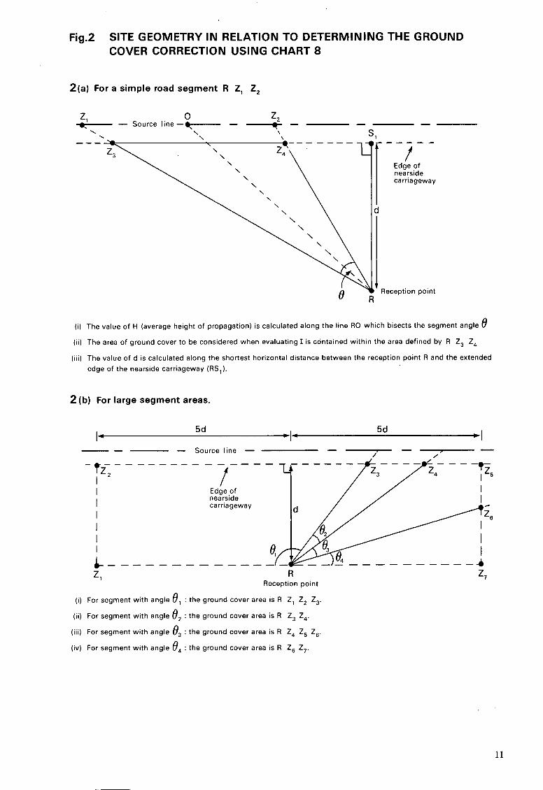
Fig.2 SITE GEOMETRY IN RELATION TO DETERMINING THE GROUND COVER CORRECTION USING CHART 8
2 ( a ) For a simple road segment R Z, 2,
- - 4 U L, r, - Source line-q- - - \
'\ \ SI \ \
(i) The value of H (average height of propagation) is calculated along the line RO which bisects the segment angle 8 (ii) The area of ground cover to be considered when evaluating I is contained within the area defined by R Z, Z,
(iii) The value of d is calculated along the shortest horizontal distance between the reception point R and the extended edge of the nearside carriageway (RS,).
2 (b) For large segment areas.
4 5d
- VI- 5d 14
-- - Source line - -r- / ,
- v - - - - - I I I I I
I Frlno nf I / / I
R Reception point
(i) For segment with angle 8, : the ground cover area is R Z, Z, Z,.
(ii) For segment with angle 8, : the ground cover area is R Z, Z,.
(iii) For segment with angle 8, : the ground cover area is R Z, Z, Z,.
(iv) For segment with angle 8, : the ground cover area is R Z, Z,.
11

20.5 In most cases when predicting for reception points 4 metres or more above ground, the presence of low walls, fences etc. may be ignored; below 4 metres screening effects such as reasonably continuous walls and other permanent features should be taken into account (but see also para 22.3).
20.6 Where the ground falls steeply away from the road, the screening effect of the road structure may also need to be taken into account by treating the edge of the structure as a barrier (see Annex 7).
21. Obstructed propagation The screening effect of intervening obstructions such as buildings, walls, purpose-built noise barriers etc* needs to be taken into account. The degree of screening depends on the relative positions of the effective source position S, the reception point R and the point B where the diffracting edge along the top of the obstruction cuts the vertical plane, i.e. normal to the road surface, containing both S and R, see Fig3(a). The region between the obstruction and the reception point is divided into the illuminated zone and shadow zone by the extended line SB, shown dotted in Fig 3(a). The degree of screening is calculated from the path difference of the diffracted ray path SBR and the direct ray path SR. Figs 3(b) and 3(c) show the calculation of the path difference depending on whether the reception point is in the illuminated zone or the shadow zone respectively. The path difference is used in Chart 9 to calculate the potential barrier correction (A). This correction is applied to the basic noise level corrected for distance according to the procedure given in para 18.
21.1 For the purposes of the Noise Insulation Regulations, it is required to calculate the path difference to the nearest 0.001 metres but the relative heights and horizontal distances need only be estimated to the nearest 0.1 metres. Chart 9a gives the polynomial expression for the value of A for both zones and should be used when calculating noise levels to the nearest 0.1 dB(A) (see para 7). However, Chart 9b may be used to estimate the value of A by rounding the value of the path difference ( 6 ) to the nearest 0.01 metres and reading the value of A from the table. Generally this will provide values of A equal to or within 0.1 dB(A) of the value obtained using the polynomial expression. However, where adjacent values of A in the table differ by more than 0.1 dB(A) the polynomial expression should be used.
21.2 The above procedure applies to all types of obstructions in calculating the potential barrier correction. The following paragraphs (22-24) deal with various types of obstructions and to the specific procedures to adopt when calculating the potential barrier correction (A).
* Hedges, bill hoardings etc should be regarded as temporary structures and their screening effect ignored.
12

Figure 3. SITE GEOMETRY TO EVALUATE THE PATH DIFFERENCE (6) FOR OBSTRUCTED PROPAGATION
Ill um i na ted zone
Diffracting edge
Edge of nearside carriageway
Shadow zone
Path difference (6) = SB+BR-SR
= SB+BR-d’
Source line
Illuminated zone
’c 3(c) SHADOW ZONE /
3(b) ILLUMINATED ZONE /
/ / /
/ / Shadow
zone / /
/ /
/
d+3.5 d+3.5 -
Path difference (6) = SB+BR-d’ Path difference(6) = SB+BR-d’
N.B. Path difference is calculated in the vertical plane,normal to the road surface, containing both R and S
13

22. Barriers Where a barrier is interposed between the noise source and reception point (either a purpose-built barrier or obstruction due to the site layout, buildings etc.) the additional correction shall be calculated using Chart 9* as outlined in para 21 and applied to the basic noise level corrected for distance according to the procedure given in para 18. The potential barrier correction is calculated in the same plane ie. normal to the road surface, as the distance correction (see Annex 8).
22.1 If the barrier is parallel to the source line but screens only part of a road segment then the barrier and the source line contained within the segment may need to be extended to enable the potential barrier correction to be calculated in the same plane, ie. normal to the road surface, as the distance correction (see Annex 9).
22.2 If the barrier is not parallel to the source line then the potential barrier correction will vary along the length of the barrier and it may be necessary to divide the barrier into a number of smaller segments. The number of segments required to calculate the screening of the barrier should be limited such that the variation in the potential barrier correction within each segment is less than 2dB(A). The potential barrier correction for each barrier segment is then determined by rotating the barrier segment about the point where the line bisecting the segment angle intersects the top edge of the barrier, so that the top edge of the barrier is parallel to the source line contained within the segment and then extended if necessary and Chart 9 applied (see Fig 4). An example of this procedure is given in Annex 10.
22.3 The additional attenuation referred to as ground absorption, para 20, is ignored when calculating the effects of barriers since the near ground rays are obstructed. However, under certain conditions (eg with low barriers erected on grassland) it is possible for these ground absorption effects to exceed the calculated screening provided by the barrier. The barrier will not raise the noise level in the screened zone, and in these circumstances the noise levels with and without the barrier should be calculated and the lower of the noise levels used (see Annexes 7 and 8).
22.4 Where more than a single barrier is interposed between the source line and the reception point a more complex procedure is required to calculate the potential barrier correction. The procedure is included in Section I1 para 35 (see Annex 11).
23. Safety fences It has been shown that conventional low safety fences of double corrugated beam construction and with a relatively small gap to the ground (mounting height of centre of beam above adjoining carriageway surface of not more than 610 mm) have broadly the same effect as noise barriers whose height is equal to the width of the solid portion of the safety fence, although the overall screening is slight. Other safety barriers of smaller cross-section, e.g. rolled hollow beams, chains, wire rope etc, or with larger gaps to the ground are to be ignored in the calculation. Since the screening effect is likely to be slight, it may be necessary to adopt the procedure given in paragraph 22.3 particularly when the ground cover is predominantly absorbent (see Annex 8).
~~ ~~
* Chart 9 gives the correction due to a massive barrier. The minimum superficial mass m (ie the mass per unit area) required to approximate this condition varies with the value of potential barrier correction (A) and for a solid barrier can be estimated from the formula m = 3 x Antilog,,, [ - (A + 10)/14] kg/m2. I t should be noted that the value of A, as derived from Chart 9, will always be negative.
14
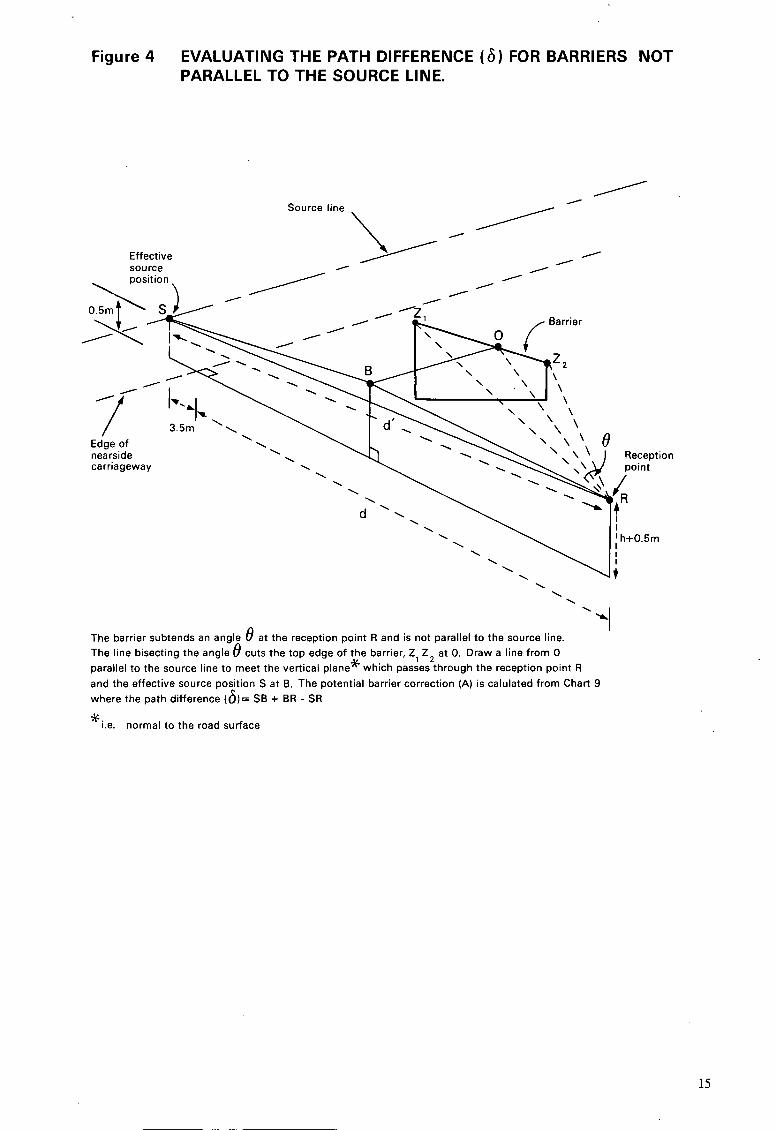
Figure 4 EVALUATING THE PATH DIFFERENCE ( 6 ) FOR BARRIERS NOT PARALLEL TO THE SOURCE LINE.
/' Source line
I I I I I
Effective source
I
carriageway
\ \ \
The barrier subtends an angle 8 at the reception point R and is not parallel to the source line. The line bisecting the angle 8 cuts the top edge of the barrier, 2, Z 2 at 0. Draw a line from 0 parallel to the source line to meet the vertical plane* which passes through the reception point R and the effective source position S at B. The potential barrier correction (A) is calulated from Chart 9 where the path difference (6)= SB + BR - SR
'i.e. normal to the road surface
15
24. Buildings To evaluate shielding due to an intervening building*, the effective height and position of the equivalent barrier shoud be determined geometrically, being defined by the intersection of two straight lines both just grazing the top edges of the building in question, one drawn from the reception point, the other drawn from the effective source position (see Annex 12). For equivalent barriers parallel to the source line the procedure given in para 22.1 applies, whereas for equivalent barriers not parallel to the source line the procedure given in para 22.2 applies.
Site layout
25. Having corrected the basic noise level from a road segment for propagation it is necessary to consider the effects of certain site layout features. Included in this part of the calculation are the effects of reflections from buildings and other hard rigid surfaces, propagation down side roads and corrections for the size of the segment. Situations where both screening and reflection effects combine, e.g. with retained cuts and dual noise barriers, require more complex correction procedures. These procedures are included in Section I1 para 36.
26. Reflection effects Reflection of noise from hard rigid surfaces adjacent to the source or in the neighbourhood of the reception point increases the noise level compared with that calculated under the above procedures, which give the free-field noise level. The ‘free-field’ noise level is appropriate where the site is open and clear and the reception point is away from other facades.
26.1 Facade effect To calculate noise 1 metre in front of a facade, a correction of +2.5 dB(A) is to be made. (Other noise calculations along side roads lined with houses but away from the facade still require the same addition of the 2.5 dB(A) because of the proximity of facades, see para 27).
26.2 Reflection f rom opposite facades Where there are houses, other substantial buildings or a noise fence or wall beyond the traffic stream along the opposite side of the road, a correction for reflection from the opposite facade facing the reception point is required. The correction only applies where the height of the reflecting surface is at least 1.5 metres above the road surface.
The correction for reflection from opposite facades is +1.5(8’/8) dB(A) where 8’ is the sum of the angles subtended by all the reflecting facades on the opposite side of the road facing the reception point, and 8 is the total angle subtended by the source line at the reception point (see Fig 5) . The above correction is required in addition to the +2.5 dB(A) facade correction described in para 26.1. For calculating the reflection correction for a reasonably uniform row of houses on the opposite side of the road see para 34.2.
* The evaluation must normally be on the basis of the built form ;IS it exists, but foreseeable changes may be taken in to account, eg where demolition without replacement i s a firm intention for the near future.
16

Figure 5 . CALCULATING THE REFLECTION CORRECTION FOR FACADES
TRAFFIC STREAM FACING THE RECEPTION POINT ON THE FAR-SIDE OF THE
Buildings
Reception point ' R
REFLECTION CORRECTION =
where e'= and 8 =
+ 1.5 (l) dB(A)
e, + e2+ e,+e, TOTAL SEGMENT ANGLE
17
27. Side roads For side roads the above correction applies only when there are houses or other substantial reflecting walls along the main road opposite the aperture of the side road and within the angle of view of the reception point. In this case however, 6 is the angle of view of the main road at the reception point defined by the aperture of the side road, and 6' is the sum of the angles subtended by all the reflecting facades on the opposite side of the main road facing the reception point contained within the total angle 6 (see Annex 13).*
28. Size of segment The noise level at the reception point from the segment of the road scheme depends upon the angle 6 subtended by the segment boundaries at the reception point. This angle is often referred to as the angle of view. The correction for angle of view is obtained using Chart 10.
Combining contributions from segments
29. The final stage of the calculation process, to arrive at the predicted noise level, requires the combination of noise level contributions from all the source segments which comprise the total road scheme**. For a single segment road scheme then, of course, there is no further adjustment to be made. For road schemes consisting of more than one segment the predicted noise level at the reception point shall be calculated by combining the contributions from all the segments using Chart 11 to give the overall noise level (L). For the purposes of the Noise Insulation Regulations each contribution should be rounded to the nearest 0.1 dB(A) in accordance with para 7. Where more than two contributions are to be combined, section (ii) of Chart 11 applies.
* Where the traffic on the side road is not negligible it will be necessary to take this into account in calculating the total noise level. Due to the proximity of walls along side roads the facade correction of +2.5 dB(A) applies at all points along the side road (para 26.1 refers). * * It is important to combine noise level contributions logarithmically when calculating the overall noise level (L).
18 -
Section II - The prediction method (additional procedures)
30. Low traffic flows The procedure given in Section I enables calculations of hourly Ll0 dB(A) and L ~ o (18-hour) dB(A) to be made for road schemes where traffic flows on any segment contained within the scheme are greater than or equal to 50 veh/h or 1000 veh/l&hour day. However, it is known that for traffic flows in the range 50 q < 200 veh/h or 1000 S Q < 4000 veh/l8-hour day, the noise level flow function takes a different form from that shown on Charts 2 and 3. For these flow ranges the noise level changes more rapidly with traffic flow than indicated. The rate at which the noise level changes with flow is also affected by the distance between the reception point and the effective source position. Consequently, for some road schemes where low traffic flows occur a further correction to the predicted noise level obtained by applying the procedure given in Section I may be needed. The following gives the method to be adopted in such cases. See Annex 14.
NB Low traffic flow segment: This term describes a road segment where the hourly traffic flow is in the range SO < q < 200 veh/h or the 18-hour traffic flow is in the range 1000 S Q < 4000 veh/l8-hour day and the shortest slant distance (d’) from the reception point to the effective source position is less than 30 metres.
Where the traffic flow on a segment is within the range quoted above but the shortest slant distance (d’) is equal to or greater than 30 metres no further correction is applied to the calculated noise level obtained following the procedure outlined in Section I.
Calculations of noise level for traffic flows below 50 veh/h or 1000 veh/l8-hour day are unreliable and measurements should be taken when evaluating such cases.
30.1 To calculate the noise level from an individual low traffic flow segment the procedure outlined below should be followed.
1. Calculate the predicted noise level for the segment (L) by applying the procedure outlined in Section I, paragraphs 12-28.
2. The corrected predicted noise level (LL) for the segment is given by
L , = L + K
where K = - 16.6 (LogloD)
and D = - 30 where d’ is the shortest slant distance between the reception point and d’ the effective source position,
and C = or Q 200 4000
depending upon whether the correction (K) is applied to an hourly Ll0 or Llo (18-hour) value respectively, and where q and Q are the hourly and 18-hour traffic flows respectively.
Chart 12 gives the correction value K.
NB The correction only applies when 50 s q < 200 veh/h or 1000 s Q < 4000 veh/l&hour day and d‘ < 30 metres, otherwise no correction should be applied.
30.2 Where a road scheme consists of one or more segments containing low traffic flows the overall predicted noise level from the road scheme is calculated by the following procedure.
1. Calculate the predicted noise level for each segment (L) by applying the procedure outlined in Section I paras 12-28.
2. For each low traffic flow segment apply the correction outlined in para 30.1.
3. Combine all the contributions from each segment using Chart 11.
NB (i) The method used for combining noise levels described above is an approxi- mation. However, although a more precise solution can be found, this tends to be rather complicated and, in most cases, the results are not significantly different from those obtained using the above procedure.
(ii) For low flows, prediction of Llo (18-hour) dB(A) using 18-hour traffic flows can differ from values obtained by averaging the hourly values over the same period. In general, predictions of Ll0 (18-hour) dB(A) for low traffic flows should be calculated, where possible, using hourly traffic flow data to obtain the eighteen, one hour, LIO values over the prescribed period and then averaging these values. It should be noted that hourly Llovalues are most sensitive to changes in traffic flow in the low flow region. For cases where the traffic flow cannot be determined accurately, the measurement method is preferred.
(iii) When determining the need to make corrections for low traffic flows special care should be taken to ensure that noise levels from non-traffic sources are substantially lower than the levels from the traffic otherwise site noise levels could be under predicted using the method (see also para 5) .
31. End of scheme Where a section of road has been improved or altered it may be necessary to predict the noise level at sites near to the end of the improved road scheme. The noise level is evaluated by treating the improved and non-improved sections of the road as separate segments. The noise level contribution from each segment at the receiver position is evaluated separately and finally combined using Chart 11. (Annex 15 gives an example calculation.)
32. Curved roads Curved roads should be broken down into several straight line segments and each segment treated separately as detailed in Section I . The separate contributions at the reception point are combined using Chart 11 to obtain the predicted noise level (see Annex 4).
33. Multiple roads including road junctions Calculation of noise from multiple roads is achieved as an extension of the procedures outlined in Section I. The contribution from each individual length of road .is calculated separately, using the appropriate mean speed (see para 14) and ignoring any speed change at the junction, and the overall predicted noise level obtained asing Chart 11. Some difficulties may be encountered, however, since the segment boundaries may not be precisely defined in all cases. In general, the location of segments will depend upon the presence of buildings and the position where the source lines of each road segment intersect. Annex 16 illustrates how segmentation of two particular junction designs could be achieved. For the roundabout site the source lines could have been drawn to intersect at different positions which would have resulted in different segment angles. In such situations the noise contribution from each road segment should be calculated for each possible segment angle and the maximum resultant predictedmoise level taken.
20

34. Houses fronting onto a main road 34.1 Screening effects Due to the need to take into account a large number of finite barriers, i t may become tedious to calculate the received noise level behind a reasonably uniform row of houses which face on to a major road especially in the case where the reception point is some distance from the row of houses (eg the noise level at the second row of houses) using the procedures in paras 22 and 24. In such cases an equivalent barrier segment can be determined whose subtended angle 8 is reduced to 0y where y is defined as
b y = a + b
where a is the mean opening between buildings and b is the mean length of building evaluated along the main road in the vicinity of the reception point. The original segment can then be treated as two separate segments whose subtended angles are Oy (the screened segment), and 0 (1 - y) which represents the unscreened portion. The two segments are treated separately and their noise level contributions combined using chart 11 to obtain the total contribution from the segment. NB. When evaluating the contribution from the unscreened segment an appropriate ground cover correction, para 20, may be required. In such cases the mean height of propagation (H) may be determined along the original segment bisector, ignoring the presence of the houses, and the proportion of absorbent ground determined from the type of ground enclosed by the original segment boundaries (see Annex 17).
34.2 Reflection effects Where a reasonably uniform row of houses exist which face the reception point on the opposite side of the traffic stream the reflection correction for opposite facades, see para 26.2, can be calculated using the value y defined above. The reflection correction is equal to + 1.5 y dB(A).
35. Multiple screening Where more than a single barrier is interposed between the source line and the reception point the following procedure shall be adopted to predict the overall noise level (see Annex 11).
(i) Where possible, segment the screened source line into single and multiple screened segments, in accordance with para 11 (see Fig 6).
(ii) For each segment, calculate the basic noise level in accordance with paras 12-16 and correct for distance in accordance with para 18.
(iii) For single screened segments, e.g. segment angle €I1 and O4 in Fig 6, calculate the potential barrier correction in accordance with para 22 and correct the values obtained in step (ii) accordingly for each segment.
(iv) For segments containing double screening, e.g. segment angle 82 calculate the potential barrier correction for each barrier separately in accordance with para 22 and combine their potential barrier corrections using the formula:-
Ac= -lOLoglo[Antiloglo(-AA/lO) + Antiloglo(-A~J/lO)-l]
where AA and AB are the potential barrier corrections derived from Chart 9 (NB values of A will be negative) such that AA 6 AB ie AA has the most negative value
21
M a n d J = ( - ) '
where M is the horizontal distance between the top edge of the barriers, and d is the shortest horizontal distance between the reception point and the edge of the nearside carriageway.
Correct the value obtained in step (ii) for the segment by adding the value Ac (NB Ac should be a negative value).
(v) For multiple screened segments, eg segment angle 03 in Fig 6, calculate the potential barrier correction for each barrier separately in accordance with para 22 and select the barrier which gives the most negative value, AA. Combine the potential barrier correction AA with each of the remaining potential barrier values, separately, as in step (iv) and select the Ac value which is most negative.
(vi) Correct the value obtained in step (ii) for the segment by adding the value Ac.
(vii) Correct the contributions from each segment to take account of reflection effects, angles of view and other site layout details and combine the values, para 29, to give the overall predicted noise level.
36. Combined screening and reflection effects Where a road is flanked on both sides by substantial reflecting surfaces such as retained walls or purpose-built noise barriers the screening performance of such barriers can be reduced due to reflection effects. The procedure to adopt when calculating the reflection correction for these situations is outlined below. * This correction is in place of and is not additional to the correction given in para 26.2.
NB (i) If the height of reflecting wall or barrier is less than 1.5 metres above the road surface no reflection correction should be applied.
(ii) Although superficially similar, the reflection effects associated with a uniform row of houses along both sides of a road are not so obtrusive. In such cases correction for reflection effects is to be made in accordance with para 34.2.
(iii) The corrections given by these procedures assume continuous, hard, reflecting surfaces. Surfaces covered with vegetation or constructed from purpose-built sound absorbing material will reduce reflection effects and where these are present noise levels will tend to be over-predicted by the method.
(iv) Where a road runs into a cutting where the sides are of earth material or where there are earth embankments alongside the road, no reflection correction is required, but see also para 36.2(i).
* Where the two carriageways are treated individually, see para 13.1, the reflection correction is calculated for each carriageway separately. The parameters used in calculating the correction will be related to the carriageway being considered.
22

Figure 6. COMBINING POTENTIAL BARRIER CORRECTIONS FOR MULTIPLE SCREENED ROAD SEGMENTS.
Source line I S
\
\ f '\ \ + \ BARRIER 1
\ E
+ D
\ I
4 \ \ BARRIER 2 \ \ \ 1
\ \ \ \ \
RZ, and RZ, are the bisectors of segments 3 and 4 respectively
U
Reception point /
Edge of nearside carriageway
I Effective source position
/ I
1- - I- I '-
/ 4- I SEGMENT 3
- 4
j SEGMENT 4 /
/
I IM13 /
I I
I 0 ' / 0
0
BARRIER 3 0
0
'/// -"
SEGMENT 1
SEGMENT 2
SEGMENT 3
SEGMENT 4
N.B.
BARRIER 1
BARRIER 1 BARRIER 2
BARRIER 1 BARRIER 2 BARRIER 3
BARRIER 3
Potential barrier correction = A,
Potential barrier correction = A, Potential barrier correction = A,
if A, < A, then using the same nomenclature as in para 35(iv) A,= A, and A,= A, and A,(the combined potential barrier correction) can be calculated with M = M,,.
Potential barrier correction = A , Potential barrier correction = A, Equivalent potential barrier correction = A,
if A, < A, < A, then using the same nomenclature as in para 35(iv) A, = A,and A, = A, or A, depending on which value gives the most negative A,value wi th M = M,, or M,3 respectively.
Equivalent potential barrier correction = A
(i) Path differences for all barriers are calculated in the vertical plane, ie normal t o the road surface, passing
through RS and used with Chart 9 to evaluate the potential barrier correction.
(ii) All potential barrier correctionsare negative values.
/ 0
23
36.1 Figures 7(a) and (b) show a section through a typical road element where dual barriers and retained cut run parallel to the source line. To calculate the noise level at the reception point, R, the following procedure should be adopted. (see Annex 18).
1. Segment the road scheme according to the procedure outlined in paragraph 11. Normally a length of road where dual barriers or walls of similar length run parallel to the source line will constitute a single segment.
NB The reflection correction is calculated in the same plane, i.e. normal to the road surface, as the distance correction and for some segments it may be necessary to extend the retaining walls and barriers together with the source line before the following procedures are applied.
2. Calculate the basic noise level and correct for distance and screening provided by the retained cut or barriers detailed in paragraphs 12-22.
3. Calculate the correction for reflections using the formula:
Correction = [1.5 + (A2 - A,) { 1 + A5 (AI - 1) } ] A4
(a) The value of A I , depends on the relative height of the screening barrier above the road surface (W), the height of the reflecting barrier above the road surface (Y), and the height of the reception point R above the road surface (a), see Fig 7(a). A, is determined in the following way:-
if Y Z= W and a > W A, = W if Y 2 W and a < W A I = a for a <1, A I = 1 i f Y < W a n d a > Y A I = Y i f Y < W a n d a < Y A I = a f o r a < l , A 1 = l .
(b) Apply Chart 13 to determine the value of A2 as a function of a and A, as a function of the horizontal distance from the reception point to the top edge of the screening barrier, (p). (c) Apply Chart 14 to determine the value of A4 as a function of the horizontal distance between the top edge of the screening barrier and the base of the reflecting barrier (E).
(d) Apply Chart 15 to determine the value of A, as a function of the angle of the reflecting barrier to the vertical (0). 4. Add the correction obtained in step 3 to the value obtained in step 2, and correct this value in accordance with the size of the segment - see paragraph 28.
5. Combine contributions from other segments using Chart 11 to obtain the predicted noise level. 36.2 The above procedure outlines the method to be adopted when calculating the reflection for typical dual barrier and retained cut situations. The following paragraphs give additional procedures to be adopted when calculating the reflection correction for some specific configurations. (i) For dual barriers where either barrier is erected on top of an earth embankment, or cut where the sides are of earth material, the reflection correction outlined in para 36.1 is applied but with A, = 0. (ii) Where a barrier is erected on top of a retained cut the reflection correction outlined in para 36.1 is applied and the relevant parameters ie W, Y and 0, where necessary, are calculated by treating the barrier and retaining wall as a single structure, see Fig 7(c). (iii) Where the retaining walls or barriers run non-parallel to the source line it is required to rotate them parallel to the source line by the method outlined in para 22.2 before applying the reflection correction para 36. I .
24

Figure 7 . EXAMPLES OF DUAL BARRIERS AND RETAINED CUTS
- -
7(a) DUAL BARRIERS.
E
(i) with vehical walls.
- - 13
\ I
Top edge of screening barrier
/ /
/ /
/ /
/ /
Effective source position
_--- 1 r Zl
- . Reception point
\ . . . \
.
Edge of nearside carriageway / s i 4 d
(ii) with sloping walls.
Top edge of screening barrier --* ’ I‘
Edge of nearside carriageway ’
I- E
N.B. Potential barrier correction (A) is calculated from the path difference ( 6 = SB + BR - SR) and ap.plying Chart 9.
. -
25
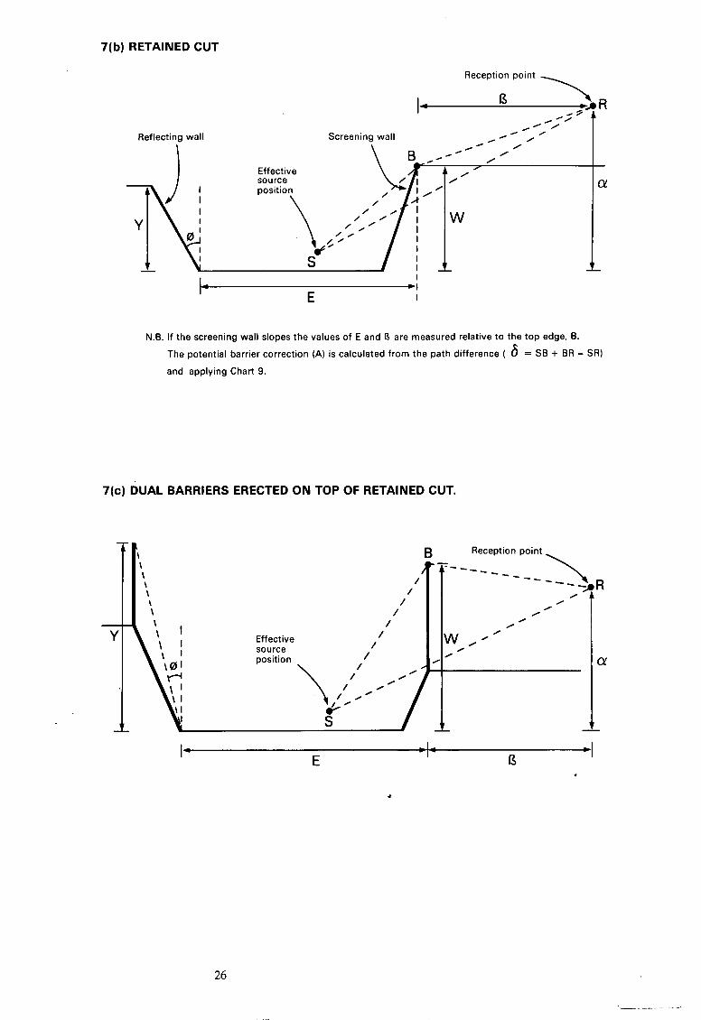
7(b) RETAINED CUT
Reflecting wall
I' E - I
I
N.B. If the screening wall slopes the values of E and I3 are measured relative to the top edge, B.
The potential barrier correction (A) is calculated from the path difference ( 6 = SB + BR - SR)
and applying Chart 9.
7 ( c ) DUAL BARRIERS ERECTED ON TOP OF RETAINED CUT.
T
R
- CY
B L \ \ \ \ \ \ \
\ I \ I k I
Reception point
- - - - - --- - -- 'I
/ 0
0 0
0 0
0 w / / 0
0
R
CY
- - - - )I E 13 I-
#
26
Section 111 - The measurement method
37. The method consists of measuring the noise from an actual flow of traffic on a road. Generally it will be required that the measurement position is close to the road so that other traffic or extraneous noises do not influence the measured level. The measured level is adjusted to give a noise level at 10 metres from the nearside carriageway edge by applying the necessary corrections in Section I. The algebraic sign of the corrections should be reversed before applying it to the measured level. The value obtained from the above procedure is the basic noise level and the calculation, as necessary, of L10 (18-hour) at the reception point is obtained using the procedures outlined in paras 17-28 of Section I.
37.1 For the purposes of the Noise Insulation Regulations and where there are no other significant noise sources in the area (or they are separately identifiable), measurements 1 metre from an eligible facade may be appropriate in such circumstances. The measured level can be used without the need to calculate the basic noise level when evaluating the Llo (18-hour) dB(A) level.
38. When to measure The measurement method may be used where:-
(i) traffic conditions fall outside the range of validity of the Charts;
or (ii) traffic or site layout conditions are sufficiently complex or unusual to make the use of standard traffic data unreasonable;
or (iii) measurement provides a more economic method of determining the particular level of traffic noise.
However, the highway authority shall use the prediction method unless’in their opinion it is inappropriate to the circumstances of the case.
39. Physical conditions for measurement The following conditions should prevail throughout the measurement period.
39.1 Road surface Measurements are to be made when the road surface in the measurement area is dry.
39.2 Wind Measurements should be made where:
(i) the wind direction is such as to give a component from the nearest part of the road towards the reception point exceeding the component parallel to the road;
(ii) the average wind speed at a height of 1.2 metres and mid-way between the road and the reception point is not more than 2 m/s in the direction from the road to the reception point;
(iii) the wind speed at the microphone in any direction should not exceed 10 m/s.
In all cases it is recommended that a wind shield be used on the microphone and that measurements should only be carried out when the peaks of wind noise at the microphone are 10 dB(A) or more below the measured value of LlO.
27

40. Measuring equipment Equipment used for the measurement of LLo should be capable of satisfying the specification given for guidance in Appendix 1. As regards calibration, evidence of general compliance with the requirements may be based upon manufacturers' published technical data but regular (not less than annual) checking is necessary to ensure that equipment is correctly calibrated. Guidance on minimum calibration requirements is given in Appendix 2.
41. Measurement procedure The following procedure should be adopted when carrying out the measurements.
41.1. Microphone position The measurement point should be chosen so that the view of the road in question is substantially unobstructed (0 > 160") and should normally be not less than 4 metres and not more than 15 metres from the nearside edge of the carriageway. The microphone should normally be placed at a height of 1.2 metres above the road surface and with the diaphragm or other sound-sensitive surface horizontal (grazing incidence). Where possible, free-field conditions should apply. However there should be no sound- reflecting surfaces (other than the ground) within 15 metres of the microphone position. Where there is doubt about whether free-field conditions prevail, particularly for the purposes of the Noise Insulation Regulations, a temporary screen to act as a facade should be erected (see also para 37.1). The screen should have an area of not less than 1 sq. metre and be positioned with its centre 1 metre behind the microphone. The screen may also assist in ensuring that extraneous noise sources do not affect the measured level. It should be noted that when a temporary screen is used the facade correction, para 26.1, should be subtracted from the measured level when evaluating the basic noise level.
41.2 Sampling times The minimum sample length tmin leading to a valid measurement of Llo depends upon the registration rate r in samples per minute (in order to ensure a sufficient overall number of samples) and on the total flow q, in vehicles per hour, passing the measuring point (in order to ensure measurements include an adequate sample of vehicles). Provided q is greater than or equal to 100 veh/h the minimum sampling time can be determined from
4000 + 120 minutes tmin = ( q - )
r
provided r is greater than 5 samples per minute and with the restriction that the sample length should not be less than 5 minutes in any one hour. For vehicle flows less than 100 veh/h the sampling rate, r , should be at least 1 sample per second and measurements should be taken for the full hour excluding time required for calibration and printer output, if required.
41.3 Traffic counts Where possible the measurements of traffic flow and composition should be concurrent with measurements of the traffic noise.
28
L

42. Analysis of data For any given sample, the noise level registrations are analysed to identify the number of registrations exceeding predetermined noise levels. These are converted to fractions of the measuring period, and Llo, the level exceeded for just 10% of the measuring period, determined by linear interpolation between the readings immediately on either side. (Care should be taken that the lower class limit of noise is used as independent variable and not the centre of the class interval.) To give adequate precision when determining the value of Llo by linear interpolation the interval between the predetermined noise levels is not to exceed 2.5 dB(A). However, systems with an inherent class-interval of 5 dB(A) may be employed provided that the analysis is repeated (eg by use of a tape recorder) with an additional 2.5 dB(A) attentuation in circuit in order to produce an effective interval of 2.5 dB(A).
42.1 Derivation of Llo (18-hour) dB(A) The above procedure enables hourly LIO dB(A) levels to be derived and the LIO (%hour) value is the arithmetic mean of the 18 one-hourly values of L ~ o covering the period 0600 to 2400 hours.
t=23
where t signifies the start time of the individual hourly L,o dB(A) values in the period 0600 to 2400 hours.
Unless measurements at the facade position have been carried out, see para 37.1, it is necessary to adjust the Llo (18-hour) value obtained above in accordance with the procedure outlined in para 37 to evaluate the Llo (18-hour) dB(A) value at the facade position.
42.2 Calculation of future values of Llo (]&hour) dB(A) To forecast the Llo (18-hour) value relating to future traffic conditions (signified Q’, V’, p’) the following procedure is adopted (where Q, V, p are the current traffic conditions).
1. From the measurement method evaluate (L) the Llo (18-hour) dB(A) value at the reception point for the current traffic conditions.
2. Calculate the correction (ALF) to take account of the change in traffic conditions.
r
29
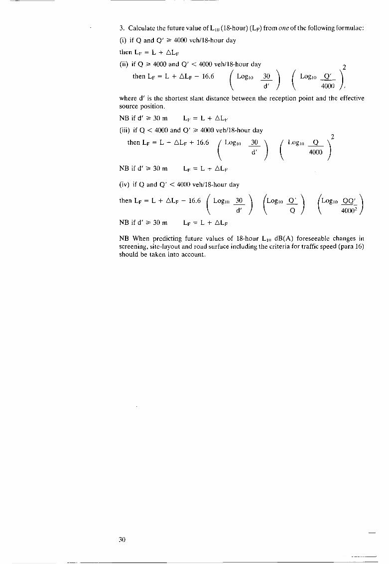
3. Calculate the future value of L lo (18-hour) (LF) from one of the following formulae:
(i) if Q and Q’ 3 4000 veh/lS-hour day
then LF = L + ALF
(ii) if Q 3 4000 and Q’ < 4000 veh/lS-hour day 2 Log10 - ( + ) ( ;i0 ), then LF = L + ALF - 16.6
where d’ is the shortest slant distance between the reception point and the effective source position.
NB if d’ 2 30 m (iii) if Q < 4000 and Q’ 2 4000 veh/lS-hour day
LF = L + ALF
,7
NB if d’ 3 30 m LF = L + ALF
(iv) if Q and Q’ < 4000 veh/lS-hour day
then LF = L + ALF - 16.6
NB if d’ 3 30 m LF = L + ALF
NB When predicting future values of 18-hour L10 dB(A) foreseeable changes in screening, site-layout and road surface including the criteria for traffic speed (para 16) should be taken into account.

Shortened measurement procedure
43. Within certain limits (see para 44) the following shortened measurement procedure may be used. Measurements of Llo are made over any three consecutive hours between 1000 and 1700 hours. Using Llo (3-hour) as the arithmetic mean of the three consecutive values of hourly Llo, the current value of Llo (18-hour) can be calculated from the relation:
Llo (18-hour) = Llo (3-hour) - 1 dB(A)
t+2
10<t<14 where Llo (3-hour) = 8 Llo (hourly),
and t signifies the start time of the individual hourly Llo dB(A) values.
The future value of Llo (18-hour) is calculated using the relevant formula given in para 42.2 above.
44. Provided that the future values of Llo (18-hour) estimated in this way are in excess of 69.0 dB(A) or are less than 66.0 dB(A) the calculated values may be used in part to determine entitlement under the Noise Insulation Regulations. Where the future value of LIO (18-hour) calculated in the shortened procedure lies within the range of 66.0-69.0 dB(A) or the increase in noise level of 1.0 dB(A) is critical (see para 6), full measurement of hourly Llo dB(A) throughout the 18-hour period is necessary, and the Llo (18-hour) dB(A) value calculated as outlined in para 42.1.
Comparative measurements
45. Comparative measurements of L10 (18-hour) may be made at a number of positions concurrently in terms of hourly Llo provided that the noise at each of the measuring positions is due to the same road carrying the same traffic under the same conditions. At one (control) position the noise should be measured through the period 0600 to 2400 hours on an average weekday. Relative measurements at the satellite positions should be made for not less than two identical periods each of at least 15 minutes duration* concurrently with measurements at the control position. The measurements at each satellite position should be taken at least 2 hours apart during the 18-hour period. Mean differences in the corresponding values of hourly Llo may then be applied to the values of Llo (18-hour) measured at the control position to determine Llo (18-hour) for the satellite positions.
* For certain vehicle flows ii longcr sampling time may bc required. Paragraph 41.2 should be applied to derive an appropriate sampling time i f longer than 15 minute periods are indicated.
31

Appendix 1 - Type specification tor measuring equipment
(a) Microphone and amplifier Over the frequency range of 63-5000 Hz the overall response of the measuring equipment including windshield, microphone, microphone preamplifier, measurement amplifier, and attenuators should comply with the A-weighting characteristics, accuracy requirements, and sensitivity to environmental factors such as temperature, relative humidity, shock and vibration, as specified for type 1 instruments in BS 5969: 1981, which is identical with IEC 651: 1979. Outside the frequency range 63-5000 Hz the overall sensitivity should not exceed the upper tolerance limit of the A-weighting characteristic specified in BS 5969: 1981.
(b) Magnetic tape recorder When direct analysis is not employed and a magnetic tape recorder is used to store audio-frequency data (as opposed to digital data) for subsequent analysis, the recordheplay system (including tape) should meet the following requirements.
(i) The gain of the recorder must be independent of input level (ie tape recorders using automatic gain control must not be used).
(ii) The device should be used in such a manner that the A-weighting characteristic is applied prior to tape recording.
(iii) The frequency-response of the complete measurement system including tape recorder should meet the tolerances specified in paragraph (a) above.
(iv) The performance of the recorder shall be such that the effective dynamic range is at least 35 dB (ie the difference between the output of the tape recorder when replaying a typical traffic noise spectrum at 3% distortion level and when replaying blank tape should be at least 35 dB). The system must be arranged so that the recorded value of Llo is at least 15 dB(A) above the inherent background noise level of the equipment and at least 10 dB(A) below the level corresponding to 3% pure-tone distortion at any frequency over the range 63-5000 Hz.
(v) The amplitude stability of a 1 kHz tone recorded at a level 10 dB below the 3% distortion level should be within k1 dB throughout any one spool of tape at the tape speed used for the noise measurement. Measurements to verify this should be made using a device with an averaging time equal to that used in the measuring chain.
(c) Characteristics of indicating instrument In principle the output from the measuring amplifier requires to be squared, averaged, converted to logarithmic form and finally displayed or digitally recorded. However, in some systems some of these operations may not be separable and it is therefore convenient to specify the overall performance of this part of the system.
The detector should operate over a minimum dynamic range of 40 dB and perform as a true mean square device to sinusoidal tone bursts having crest factors of up to 3 over the dynamic range corresponding to 50 to 85 dB(A) within an accuracy of k 0.5 dB.
The effective averaging time should be 250 milliseconds with tolerances of + 250 ms and -150 ms.
Note 1: A convenient means of checking compliance with the averaging time requirements is to apply $-octave band-limited white noise centred on a frequency of 500 Hz to the input of the detector and determine the standard deviation of the indicated level about the mean level. For a device complying with the above averaging time requirements the standard deviation of at least 500 independent samples of noise level should fall in the range 0.55 to 1.20 dB.
32
Note 2: An instrument complying with Section 7 . 2 of BS 5969: 1981 with dynamic characteristics designated F is deemed to comply with these requirements.
Note3: Logarithmic level recorders with 25 dB potentiometer, writing speed set to 100 mm/s and with a lower limiting frequency of 20 Hz are deemed to comply with these requirements.
(d) Level resolution of digital recording system In order to achieve adequate overall precision both in calibration and measurement the system should be generally capable of indicating changes in level of 0.5 dB(A).
33
Appendix 2 - Calibration of equipment
(a) On-site calibration Immediately prior to and following each session of work the overall sensitivity of the electroacoustical system should be checked using an acoustic calibrator generating a known sound pressure at a known frequency. Measurements may be accepted as valid only if calibration levels agree within 1 dB.
Note I : Sometimes a pistonphone operating at a nominal level of 124 dB at a frequency of 250 Hz is used for this purpose. As this level is outside the range required for traffic noise measurements, it will be necessary to introduce known additional attenuation (e.g. using a ‘range-switch’). Care will therefore need to be exercised when interpreting the calibration signals and it is recommended that the same attenuation (e.g. 50 dB) be adopted as routine. Attention is also drawn to the fact that where the A-weighting network is permanently connected in circuit due allowance must also be made for the relative response of the A-weighting network at the frequency used (e.g. -8.6 dB at 250 Hz).
Note 2: Where a tape recorder forms part of the measuring chain and is used to store audio-frequency data it is a requirement that, in addition to the above, a constant calibration signal corresponding to a known sound pressure level be applied at the beginning and end of each individual spool of tape used. A tape-recorded sample may be accepted as valid only if at the time of analysis the indicated levels of the two calibrating signals agree within 1 dB.
(b) System calibration To ensure overall measurement precision, within twelve months immediately prior to the measurement the overall system should have been directly compared with an independent reference system. This comparison is most easily effected by using both to measure and analyse the same noise sample. Likewise, the output level of the acoustic calibrator referred to in Appendix 2(a) should also have been checked by direct comparison with an independent reference device.
34
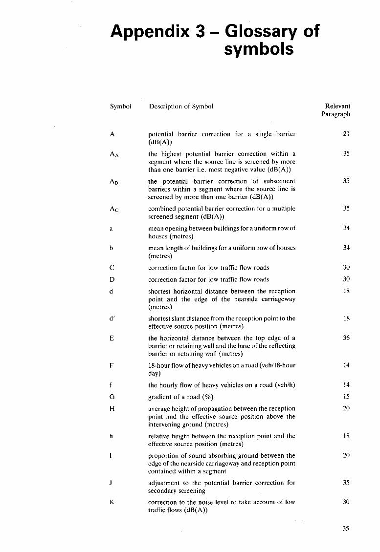
Appendix 3 - Glossary of symbols
Symbol Description of Symbol
A potential barrier correction for a single barrier
AA the highest potential barrier correction within a segment where the source line is screened by more than one barrier i.e. most negative value (dB(A))
AB the potential barrier correction .of subsequent barriers within a segment where the source line is screened by more than one barrier (dB(A))
combined potential barrier correction for a multiple screened segment (dB(A))
mean oper,ing between buildings for a uniform row of houses (metres)
mean length of buildings for a uniform row of houses (metres)
correction factor for low traffic flow roads
correction factor for low traffic flow roads
shortest horizontal distance between the reception point and the edge of the nearside carriageway (met res)
shortest slant distance from the reception point to the effective source position (metres)
the horizontal distance between the top edge of a barrier or retaining wall and the base of the reflecting barrier or retaining wall (metres)
18-hour flow of heavy vehicles on a road (veh/l8-hour
the hourly flow of heavy vehicles on a road (veh/h)
gradient of a road (%)
average height of propagation between the reception point and the effective source position above the intervening ground (metres)
relative height between the reception point and the effective source position (metres)
proportion of sound absorbing ground between the edge of the nearside carriageway and reception point contained within a segment
(dB(A))
AC
a
b
C
D
d
d'
E
F day)
f
G
H
h
I
J
K
adjustment to the potential barrier correction for secondary screening
correction to the noise level to take account of low traffic flows (dB(A))
Relevant Paragraph
21
35
35
35
34
34
30
30
18
18
36
14
14
15
20
18
20
35
30
35

Symbol
L
L F
ALF
LL
M
P
PI
Q Q'
9 r
t
tmin
V
V'
AV
W
Y
OL
P
Y
AI -A5
36
Description of Symbol
the noise level, L,o hourly or Ll0 (18-hour), dB(A) from a road segment or road scheme
L ~ o (18-hour) dB(A) level from a road for future traffic conditions
correction to the noise level to take account of future changes in traffic conditions (dB(A))
corrected contribution to the noise level from low flow traffic (dB(A))
the horizontal distance between the top edge of the barrier with the highest potential barrier correction and the top edge of subsequent barriers (metres)
percentage of heavy vehicles (%)
percentage of heavy vehicles for future traffic condi- tions (%)
18-hour traffic flow (veh/Whour day)
18-hour traffic flow for future traffic conditions (veh/lS-hour day)
hourly traffic flow (veh/h)
registration rate for sampling the noise level when measuring Llo dB(A) (samples/minute)
start time of the individual hourly Ll0 dB(A) values (hours)
the minimum sampling length, in minutes, required for a valid measurement of L10 dB(A)
mean speed of traffic on a road (km/h)
mean speed of traffic for future traffic conditions (km/h)
reduction in mean traffic speed on a road due to gradient (km/h)
height of screening barrier or retaining wall above road surface (metres)
height of reflecting barrier or retaining wall above road surface (metres)
height of reception point above road surface (metres)
the horizontal distance from the reception point to the top edge of the barrier or retaining wall (metres)
correction to the angle of view subtended by a uniform row of houses
parameters used for calculating the reflection correc- tion for dual barriers and retained cuts
Relevant Paragraph
29
42
42
30
35
14
' 42
13
42
13
41
42
41
14
42
14
36
36
36
36
34
36

Symbol Description of Symbol
6 path difference between the direct ray and diffracted ray due to screening of the source line (metres)
angle of view of a segment (degrees)
combined angle of view of reflecting surfaces on the farside of the traffic stream facing the reception point (degrees)
angle of the reflecting barrier or retaining wall to the vertical (degrees)
e 0'
0
Relevant Paragraph
21
28
26
36
37

CHART 1 FLOW CHART FOR PREDICTING NOISE FROM ROAD SCHEMES
Ground cover correction
I Stage 1 - Divide road scheme into segments I
Screening correction
/ I
Calculate noise level contribution from a segment
I Stage 2 - Basic noise level I Select hourly L,, or L,, ( 1 8- Hour)
Flow Speed Percentage heavies Gradient Road surface
I Stage 3 - Propagation I I
Distance Co rrect io n
I . I Stage 4 - Site layout I
I Correct for reflections I I ~ p p ~ y angle of view correction I
I Stage 5 - Combine contributions from all seaments
- ~~
Predicted noise level
38
-

U
s 0 4 LL * 3 0 I
4 a
3 0 I- LL 0
cy tr
0 (P c
0 0
8 F
0 0 5:
hl
c- L 3
0 0 cn In lu
.-
m
39

0 0 hl
0 0 s
0
U 3 0 T 00 r
cn r a W I-
r W
- > lu U L
0 In
0 hl
0 r
3 0 r
c, v
d
- lu
0 I- c,
In
hl
3 m U
d 0
A L 3 0 L
- a, > a, - .. .- 0 L
40

Chart 4 CORRECTION FOR MEAN TRAFFIC SPEED V AND PERCENTAGE HEAVY VEHICLES p
a v) a U S a > > > m a S
- .-
20 50 100 130
Mean traffic speed V(km/h)
Correction = 33 Log,, (V + 40 + 7 500 ) + 10 Log,, (1 +? ) - 68.8 dB(A)
41
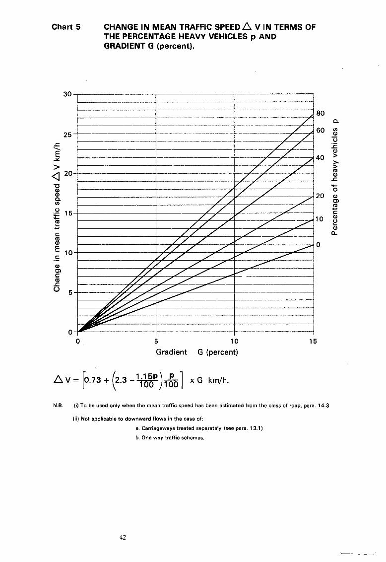
~~
Chart 5 CHANGE IN MEAN TRAFFIC SPEED A V IN TERMS OF THE PERCENTAGE HEAVY VEHICLES p AND GRADIENT G (percent).
80 Q
Y- 0
0
" I
0 I
5 I
10 I
15
Gradient G (percent)
15') ] x G km/h. -100 100 N.B. (i) To be used only when the mean traffic speed has been estimated from the class of road, para. 14.3
(ii) Not applicable to downward flows in the case of:
a. Carriageways treated separately (see para. 13.1 )
b. One way traffic schemes.
42
~

Chart 6 CORRECTION FOR GRADIENT G
+6
+5
+4 3 a U
+2
+1
0
I-
-
d I
!
I j
5 10
Gradient G (percent)
15
Correction = 0.3 G dB(A)
43

I- k 2
n2 W O
2 p o a
0 m
0 0 €9
0 In hl
L
8 - -:F h l - E
C tg: 0, L t %
0 I
-?-
44

\ "
0 c
Ln 0
L
.c 0
I
U rn - U A
a I 0 r
W s 1 ,-I
II 2
!-
a
P x 8 a
?la U
V r
,vi
? VI
0
0 U L
0 II 2
I- P x a a 0 U
VI $la A\ I
L
0 U
45
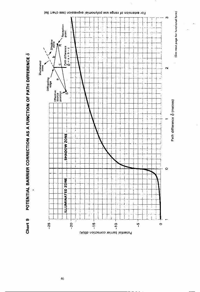
a a v)
2 0 F 0 w U U 0 0 U W z a 3
L
Lc 0 Q 0) 9 n
4-
X Q C Q 0)
",
!k U
5 m L
0
46

Chart 9a Polynomial expressions for potential barrier correction Potential barrier correction A = A,) + Alx + A2 x2 + . . . + A, x" where x = Loglo 6 (6 being the path difference in metres between the direct and diffracted rays), the coefficients A, being given in the table below.
Shadow zone Illurninured zone
- 15.4 -8.26 -2.787 -0.831 -0. I98 +O. 1539 +O. 12248 +0.02175
Range of validity -3 c x 6 + 1.2
0 +0.109 -0.815 +0.479 + 0.3284 +0.04385
- 4 s x s o
Outside the above ranges of validity the potential barrier correction is defined as follows:
Shadow zone Illurninured zone
For x < -3 A = -5.0 For x <-4 A = -5.0 For x >1.2 A = -30 Forx>O A = 0
Chart 9b Potential barrier correction A* dB(A) for path differences (6 = i + j)** calculated to the nearest 0.01 metres.
j -
I
0.0 0.1 0.2 0.3 0.4 0.5 0.6 0.7 0.8 0.9 1 .0 1.1 1.2 1.3 1.4 1.5 I .6 1.7 1.8 1.9 2.0
0.0 0.1 0.2 0.3 0.4 0.5 0.6
0.00 0.01 0.02 0.03 0.04 0.05 0.06 0.07 0.08 0.09
SHADOW ZONE 5.0 6.4 7.1 7.6 9.3 9.5 9.7 9.8
10.8 10.9 11.0 11.1 11.7 11.8 11.9 12.0 12.5 12.6 12.6 12.7 13.1 13.2 13.3 13.3 13.7 13.7 13.8 13.8 14.2 14.2 14.3 14.3 14.6 14.7 14.7 14.7 15.0 15.1 15.1 15.1 15.4 15.4 15.5 15.5 15.7 15.8 15.8 15.8 16.1 16.1 16.1 16.2 16.4 16.4 16.4 16.5 16.7 16.7 16.7 16.8 16.9 17.0 17.0 17.0 17.2 17.2 17.3 17.3 17.5 17.5 17.5 17.5 17.7 17.7 17.8 17.8 17.9 18.0 18.0 18.0 18.2 18.2 18.2 18.2
ILLUMINATED ZONE 5.0 3.5 2.8 2.3 1 . 1 1.0 . 1.0 0.9 0.6 0.5 0.5 0.5 0.3 0.3 0.3 0.3 0.2 0.2 0.2 0.2 0.1 0.1 0.1 0.1 0.1 0. I 0.1 0.1
7.9 10.0 11.2 12.1 12.8 13.4 13.9 14.4 14.8 15.2 15.5 15.9 16.2 16.5 16.8 17.1 17.3 17.6 17.8 18.0 18.3
2.0 0.8 0.5 0.3 0.2 0.1 0.1
8.2 10.1 11.3 12.1 12.8 13.4 13.9 14.4 14.8 15.2 15.6 15.9 16.2 16.5 16.8 17. I 17.3 17.6 17.8 18.1 18.3
1.8 0.8 0.4 0.3 0.2 0.1 0.1
8.5 10.3 11.4 12.2 12.9 13.5 14.0 14.5 14.9 15.3 15.6 15.9 16.3 16.6 16.8 17.1 17.4 17.6 17.8 18.1 18.3
1.6 0.7 0.4 0.2 0.1 0.1 0.0
8.7 10.4 11.5 12.3 13.0 13.5 14.0 14.5 14.9 15.3 15.6 16.0 16.3 16.6 16.9 17.1 17.4 17.6 17.9 18. I 18.3
1.5 0.7 0.4 0.2 0.1 0.1 0.0
9.0 10.5 11.6 12.4 13.0 13.6 14.1 14.5 14.9 15.3 15.7 16.0 16.3 16.6 16.9 17.2 17.4 17.7 17.9 18.1 18.3
1.3 0.6 0.4 0.2 0.1 0.1 0.0
9.2 10.6 11.7 12.4 13.1 13.6 14. I 14.6 15.0 15.4 15.7 16.0 16.3 16.6 16.9 17.2 17.4 17.7 17.9 18.1 18.4
1.2 0.6 0.3 0.2 0.1 0.1 0.0
* Values of A are negative
e.g. where the reception point is in the shadow zone and 6 = 1.45 metres: * * then i = 1.4 and j = 0.05 from the table the value of A is - 16.8 dB(A).
47

0
0 0 hl
0 U
8 3 5 W
W
U 0 2 0
LL
-
0 r
U? 0 hl +
0 hl
v)
'hl
3 0, > .-
w- 0 Q)
OY C
- a
0 r 4 m
U
0 00 F
\ m
C 0
0
0 0
.- c
2 L

Chart 11 PROCEDURE FOR COMBINING NOISE LEVELS.
3 +3 m U a > a
- - .- % +2 0 C
a L 0
0
U
L
.- I +1 .I-
a 0 0 2 4 6 8 10
Difference between two noise levels A d B (A)
(i) Given two noise levels L and L - A then the combined level is L + 1 0 Log,,[l + Antilogl,(-A/,O)] dB(A)
which can be evaluated using the above chart.
12 14 16
(ii) With n component noise levels L,, L,, ......, Ln the combined noise level due to all n components is given by
L = 10Log,,[f An t i l og , , (Ln /~o ) ] dB(A) 1
49
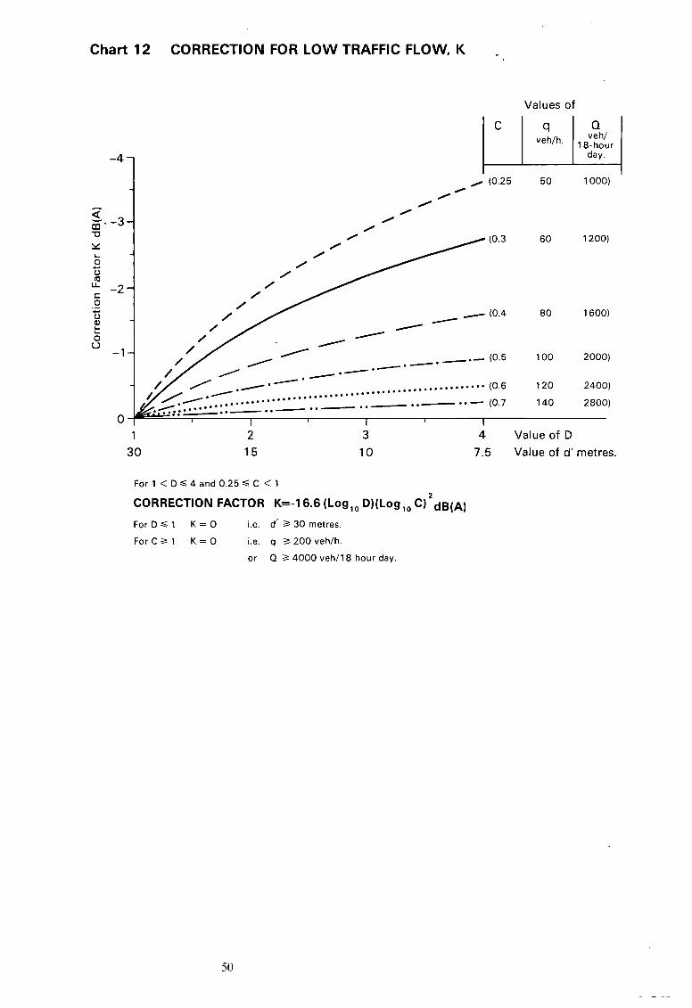
Chart 12 CORRECTION FOR LOW TRAFFIC FLOW, K
Values of
-4
z z. -3 U Y
0 0 m L
C 0 0
L
*-’
-2 .- w
2 L 0 0
-1
0 1 30
18-hour U (0.25
/ 0 -
0 0
0
50
60
8 0
100
120
140
1000)
1200)
1600)
2000)
2400)
2800)
2 15
3 10
4 Value of D 7.5 Value of d’ metres.
For 1 < D S 4 a n d 0.25 S C < 1
CORRECTION FACTOR K=-16.6 (Log,, D)(Log,, C ) ’ ~ B ( A )
F o r D S l K = O i.e. d’ 2 30 metres.
F o r C 3 - 1 K = O i.e. q 3 200 veh/h.
or Q b 4000 veh / l8 hour day.
50

a I- z 5 n z 0 E w 0 w U LL 0
0 a0 0 b
0 (0
0 v)
0 t
0 m
0 N
0 - r
I 2 I 2 I 0 - 0 0 +
v io~3 .e~ U O ! J W J O ~ E
v)
2 w
E d
0 U a 0 C
0
d
.- w
E! E E 2
U
LC
c C 0 Q C 0
Q a U
.-
.- c
2 LC 0 a U C m v) w .- n
v)
E
a U-
2
n
4-
E m
a > 0 m C 0 Q C 0
Q a 0
w .-
.- w
2
2 + 0
0 al I .-
51

Chart 14 CORRECTION FACTOR A, IN TERMS OF DISTANCE, E. [To be used in conjunction with Charts 13 and 151
Distance between diffracting edge and base of reflecting wall, E metres
CORRECTION FACTOR A4 = Log,,,[1+(270/E)] for E < 30,
for E > 70,
A4= 1
A 4 = 0.69
52

Chart 15 CORRECTION FACTOR As FOR ANGLE OF THE REFLECTING WALL TO THE VERTICAL TO BE USED IN CONJUNCTION WITH CHARTS 13 to 14.
VI
a
+ 0 a CJ) C m
0
-
L
+
i L 0 0
0 2 4 6 8 10 12 14
Angle of wall to vertical @ (degrees)
Correction Factor A5 = Exp(-O.OlS@')
where @5 = angle of the reflecting wall to the vertical in degrees.
53

Chart 16a - Traffic Forecast Table Light vehicles (1525kg or less unladen weight) Percentage change over b m e year
Future Base year year
1986 1987 1988 1989 1990 1991 1992 1993 1994 1995 - - ~ - - ~ - ~ ~ ~
1986 1987 1988 1989 1990 1991 1992 1993 1994 1995 1996 1997 1998 1999 2000 200 1 2002 2003 2004 2005 2006 2007 2008 2009 2010 201 1 2012 2013 2014 2015 2016 2017 2018 2019 2020 202 1 2022 2023 2024 2025
0 3 7
10 13 16 18 21 23 25 27 29 31 33 35 31 39 40 42 44 46 47 49 51 52 54 55 57 59 60 62 63 65 66 68 69 71 72 74 75
0 0 3 6 9
12 14 17 19 21 23 25 27 29 31 32 34 36 38 39 41 43 44 46 47 49 50
. 52 54 55 57 58 60 61 62 64 65 67 68 70
0 0 0 3 6 9
I I 13 15 17 19 21 23 25 26 28 30 32 33 35 37 38 40 41 43 44 46 47 49 50 52 53 55 56 57 59 60 62 63 64
0 0 0 0 3 5 8
10 12 14 16 18 19 21 23 25 26 28 30 31 33 34 36 31 39 40 42 43 44 46 47 49 50 51 53 54 56 57 58 60
0 0 0 0 0 2 5 7 9
I I 12 14 16 18 19 21 23 24 26 27 29 30 32 33 35 36 38 39 40 42 43 44 46 47 48 50 51 52 54 55
0 0 0 0 0 0 2 4 6 8
10 12 13 15 17 18 20 21 23 25 26 27 29 30 32 33 34 36 31 38 40 41 42 44 45 46 48 49 50 51
0 0 0 0 0 0 0 2 4 6 8 9
11 12 14 16 17 19 20 22 23 25 26 27 29 30 32 33 34 36 31 38 39 41 42 43 45 46 41 48
0 0 0 0 0 0 0 0 2 4 5 7 9
10 12 13 15 16 18 19 21 22 24 25 26 28 29 30 31 33 34 35 37 38 39 40 42 43 44 45
0 0 0 0 0 0 0 0 0 2 3 5 7 8
10 11 13 14 16 17 19 20 21 23 24 25 27 28 29 30 32 33 34 35
.37 38 39 40 41 43
0 0 0 0 0 0 0 0 0 0 2 3 5 6 8 9
I I 12 14 15 17 18 19 21 22 23 24 26 21 28 29 31 32 33 34 35 37 38 39 40
54

Chart 16b - Traffic Forecast Table Heavy vehicles (over 1525kg unladen weight) Percentage change over base year
Fitrure Base yecir yeor
1986 I987 1988 1989 1990 1991 1992 I993 1994 1995 - ~ ~ ~ - ~ - - - ~
1986 I987 I988 1989 1990 1991 I992 I993 I994 1995 1996 I997 1998 1999 2000 2001 2002 2003 2004 2005 2006 2007 2008 2009 2010 201 1 2012 2013 2014 2015 2016 2017 2018 2019 2020 202 1 2022 2023 2024 2025
0 1 2 2 3 4 5 5 6 7 7 8 9
10 10 I I I I 12 12 13 13 14 14 14 14 15 15 1.5 16 16 16 16 17 17 17 18 18 18 18 19
0 0 1 2 2 3 4 4 5 6 7 7 8 9 9
10 10 I I 12 12 12 13 13 13 14 14 14 14 15 1.5 1.5 16 16 16 16 17 17 17 17 18
0 0 0 1 1 2 3 4 4 5 6 6 7 8 8 9
10 10 I I 11 11 12 12 12 13 13 13 14 14 14 14 15 15 IS 15 16 16 16 17 17
0 0 0 0 I 1 2 3 4 4 5 6 6 7 8 8 9 9
10 10 11 11 11 12 12 12 12 13 13 13 14 14 14 14 15 15 15 15 16 16
0 0 0 0 0 1 1 2 3 3 4 5 6 6 7 7 8 9 9
10 10 10 10 11 11 11 12 12 12 12 13 13 13 13 14 14 14 15 15 15
0 0 0 0 0 0 1 1 2 3 3 4 5 6 6 7 7 8 8 9 9 9
10 10 10 11 11 11 11 12 12 12 12 13 13 13 14 14 14 14
0 0 0 0 0 0 0 I I 2 3 3 4 5 5 6 6 7 8 8 8 9 9 9 9
10 10 10 11 I I 11 11 12 12 12 12 13 13 13 13
0 0 0 0 0 0 0 0 I 1 2 3 3 4 5 5 6 6 7 7 8 8 8 8 9 9 9
10 10 10 10 11 11 I I 11 12 12 12 12 13
0 0 0 0 0 0 0 0 0 1 1 2 3 3 4 5 5 6 6 7 7 7 7 8 8 8 9 9 9 9
10 10 I0 10 11 11 11 11 12 12
0 0 0 0 0 0 0 0 0 0 1 1 2 3 3 4 4 5 5 6 6 6 7 7 7 8 8 8 8 9 9 9 9
10 10 10 10 11 I I 11
55

Annexes 1 - 18
The following annexes are included to illustrate the methodology. In all cases the road surface is assumed to be impervious with a zero correction for texture depth.
Previous page is blank 57

Annex. 1 ENTITLEMENT TO INSULATION UNDER THE NOISE INSULATION REGULATIONS 1975
CASE. 1. 1 (a) BEFORE IMPROVEMENT 1 (b) AFTER IMPROVEMENT
(within 15 years)
Improved highway L’A
CASE. 2. 2(a) BEFORE IMPROVEMENT
1
2(b) AFTER IMPROVEMENT (within 15 years)
1
New highway L’A
CASE. 3. 3(a) BEFORE IMPROVEMENT
3 (b) AFTER IMPROVEMENT (within 15 years)
.. . . . . .
58

ANNEX 1. ENTITLEMENT TO INSULATION UNDER THE NOISE INSULATION REGULATIONS 1975
The following definitions apply when considering the conditions for entitlement (see para 6).
Prevailing Noise Level (PNL) = 10 Loglo (Antiloglo- + Antiloglo -)
where LA =
LB =
LA LB 10 10
noise level from a highway or highways which are to be altered noise level from all other highways in the vicinity immediately before works to alter LA begin.
L‘B 10
L’A + Antiloglo -) Relevant Noise Level (RNL) = 10 Log10 (Antiloglo - 10
where L’A =
L’B =
maximum noise level, within 15 years, from altered highways and/or from completely new highways. maximum level from all other highways within 15 years.
Taking the above definitions a property will be eligible for insulation when
(i) RNL 2 68 dB(A) (ii) RNL - PNL 5 + 1.0 dB(A)
(iii) RNL - L’B 3 + 1.0 dB(A) For the purposes of illustration 3 cases are detailed below and a plan of each site is shown opposite. CASE 1. To calculate whether there is entitlement at No 6. The noise levels at lm from facade are
[NB 67.5 dB(A) and above is rounded up to 68 dB(A)]
Chart 11 Combined Noise Level PNL = 67.2 dB(A)
Chart 11 Combined Noise Level RNL = 69.8 dB(A)
1 1
LA = 64.2 dB(A)
LB = 64.1 dB(A)
L’A = 67.1 dB(A)
L’B = 66.4 dB(A) (i) RNL = 70 dB(A)
(ii) RNL - PNL = 2.6 dB(A) (iii) RNL - LIB = 3.4 dB(A) In this case there is possible entitlement, subject to Regulation 4. CASE 2. To calculate whether there is entitlement at No 1. The noise levels at l m from facade are
(rounded to the nearest whole number)
LA = 0 (A new highway is to be constructed) LB = 70.1 dB(A) Therefore PNL = 70.1 dB(A)
Chart 11 Combined Noise Level RNL = 68.7 dB(A) 1 L’A = 66.1 dB(A)
L’B = 65.2 dB(A) (i) RNL = 69 dB(A)
(ii) RNL - PNL = -1.4 dB(A) (iii) RNL - L ’ B = 3.5 dB(A) There is no entitlement since the second condition is not met. The traffic has been moved away from the property and the noise level reduced. CASE 3. To calculate whether there is entitlement at No 3. The noise levels at l m from the facade are
(rounded to the nearest whole number)
LA = 57.7 dB(A) 1 Chart 11 Combined Noise Level PNL = 67.6 dB(A) LB = 67.1 dB(A) J L1 = 61.7 dB(A)
L2 = 55.1 dB(A) L’A =.62:6 dB(A)
L’B = 69.3 dB(A)
Chart 11 Combined Noise Level L’A = 62.6 dB(A)
Chart 11 Combined Noise Level RNL = 70.1 dB(A)
1 i
(i) RNL = 70 dB(A) (ii) RNL - PNL = +2.5 dB(A)
(rounded to the nearest whole number)
(iii) RNL - L’B = +0.8 dB(A)
There is no entitlement since the third condition is not met. The actual contribution to the total noise level - from the improved road and the new road is 0.8 dB(A).
59

Annex. 2 HORIZONTALLY SEPARATED CARRIAGEWAYS.
PLAN VIEW
......................... 1 -- - - - - - - -- -
Sniirre l ine /
t Gardens Low wall
.........................*.*... ....................................... Pavement /Edge of nearside carriageway
-- - --------- -- - - - - Nearside carriageway
Source line 4:rside carriageway Effective edge of farside carriageway _ _ _ _ _ - / ---- --- - - - - - --
Pavement Farside kerb O O O b O 0 0 0 0 0 0 0 0 0 0 0 b 0 0 0 0 l 0 0 0 0 0 0 0 0 0 0 0 0 0 0 0 0 0 0 0 0 0 0 0 0 0 0 0 0 0 0 0 0 0 0 0 0 0 0 0 0 0
Brick Wall /
CROSS - SECTION AA'
8m
z, Farside carriageway
,,Brick Wall
8-i-
Key: R - Reception point L A
6m
Z 1
S, - Source position segment 1 S, - Source position segment 2
- Absorbent ground cover z, - Non-absorbent ground cover
8m
Z l L
Nearside carriageway Central reservation
0.5m Low \wall
c C 0,
i m a
Segment 1: H = 0.5(1 + 3.5) = 2.25m
Percentage of absorbent ground = g x 100 M 67 VO ; I.= 0.75 4
Segment 2: H = 2.25m
Percentage of absorbent ground =r x 100% 48% ; I = 0.50 4 + 6
60
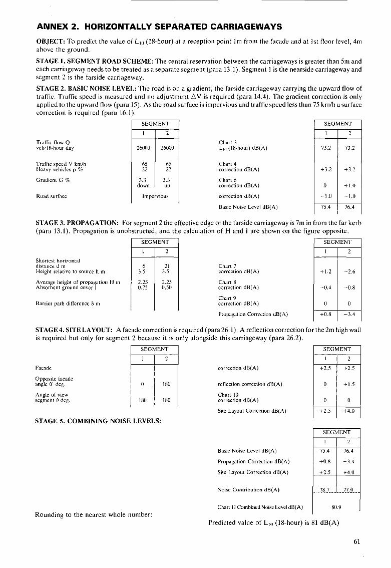
ANNEX 2. HORIZONTALLY SEPARATED CARRIAGEWAYS
OBJECT: To predict the value of Llo (18-hour) at a reception point I m from the facade and at 1st floor level, 4m above the ground.
STAGE 1. SEGMENT ROAD SCHEME: The central reservation between the carriageways is greater than 5m and each carriageway needs to be treated as a separate segment (para 13.1). Segment 1 is the nearside carriageway and segment 2 is the farside carriageway.
STAGE 2. BASIC NOISE LEVEL: The road is on a gradient, the farside carriageway carrying the upward flow of traffic. Traffic speed is measured and no adjustment AV is required (para 14.4). The gradient correction is only applied to the upward flow (para 15). As the road surface is impervious and traffic speed less than 75 km/h a surface correction is required (para 16.1).
Traffic flow Q vch/l8-hour day
Traffic speed V kmlh Heavy vehicles p %
Gradient G 5%
Road surface
SEGMENT I I
26000
65 22
3.3 down
26000
22
3.3 UP
Chart 3 Lj0 (IS-hour) dB(A)
Chart 4 correction dB(A)
Chart 6 correction dB(A)
correction dB(A)
Basic Noise Level dB(A) I Impervious
SEGMENT
+3.2 +3.2
STAGE 3. PROPAGATION: For segment 2 the effective edge of the farside carriageway is 7m in from the far kerb (para 13.1). Propagation is unobstructed, and the calculation of H and I are shown on the figure opposite.
Shortest horizontal distance d m Height relative to source h m
Average height of propagation H m Absorbent ground cover I
Barrier path difference 6 m
SEGMENT
1 1 2
3.: I 32;
2.25 0.75
2.25 0.50
Chart 7 correction dB(A)
Chart 8 correction dB(A)
Chart 9 correction dB(A)
Propagation Correction dB(A)
SEGMENT
I
+1.2
-0.4
0
+0.8
2
-2.6
-0.8
0
-3.4
STAGE 4. SITE LAYOUT: A facade correction is required (para 26.1). A reflection correction for the 21-13 high wall is required but only for segment 2 because it is only alongside this carriageway (para 26.2).
Facade Correction dB(A)
Opposite facade angle 8’ deg. reflection correction dB(A) +1.5
Angle of view Chart 10 segment 0 deg. 180 180 correction dB(A)
Site Layout Correction dB(A) +2.5 +4.0
STAGE 5. COMBINING NOISE LEVELS: SEGMENT
Basic Noise Level dB(A)
Propagation Correction dB(A) -3.4
Site Layout Correction dB(A) +2.5 +4.0
Rounding to the nearest whole number:
Noise Contribution dB(A)
Chart 1 1 Combined Noise Level dB(A)
Predicted value of LlO (18-hour) is 81 dB(A)
61
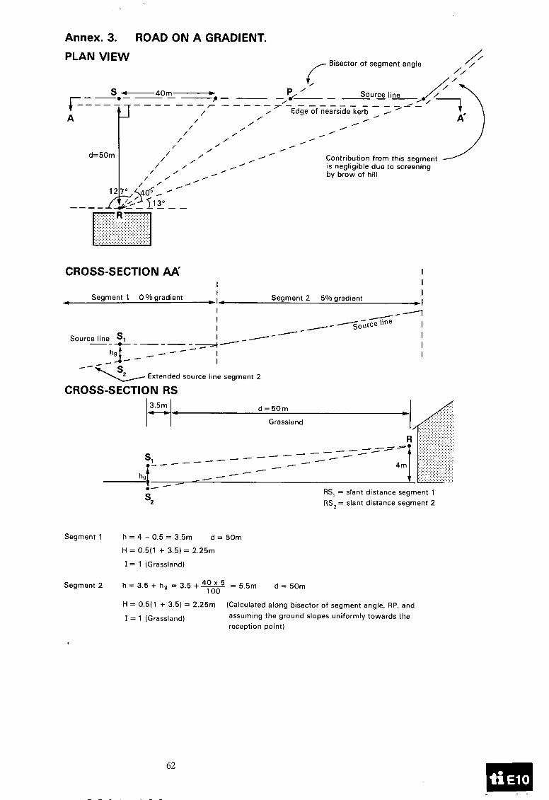
Annex. 3. PLAN VIEW
ROAD ON A GRADIENT.
0 , ’ / . / . . /
/ . / 0
/ /
/ 0 Contribution from this segment / . , is negligible due to screening
/ /
/ ’ / . d=50m
, . by brow of hill / ’
, / ’
0 / ’ ,
CROSS-SECTION AA‘ I I I
4 b I 4 Segment 2 5% gradient +I Segment 1 0 O/o gradient
I -4 I I /-,--o;‘s I
I *- I I I I
Source line Si I -/- -- +----- _--- hgf - - - - --%
Extended source line segment 2
CROSS-SECTION RS d = 5 0 m
Grassland
RS, = slant distance segment 1 RS,= slant distance segment 2
Segment 1
Segment 2
h = 4 - 0.5 = 3.5m
H = 0.5(1 + 3.5) = 2.25m
I = 1 (Grassland)
d = 50m
h = 3.5 + hg = 3.5 +U = 5.5m d = 50m 100
H = 0.5( 1 + 3.5) = 2.25m
I = 1 (Grassland)
(Calculated along bisector of segment angle, RP, and assuming the ground slopes uniformly towards the reception point)
62

ANNEX 3. ROAD ON A GRADIENT'
70 10
OBJECT: To predict the value of Llo (18-hour) at a reception point l m from the facade and at 1st floor level, 4m above the ground.
STAGE 1. SEGMENT ROAD SCHEME: The road scheme is divided into three segments. Segment 1 contains part of the road with zero gradient. Segment 2 contains part of the road with 5% gradient. Segment 3 contains the remaining part of the road screened by the intervening ground, its contribution is negligible and ignored in the calculation.
STAGE 2. BASIC NOISE LEVEL: The road is classified as a single carriageway with a 50 mph speed limit. Segment 2 has a gradient with an estimated speed of 70 km/h, an adjustment AV is required (para 14.3). Traffic speeds are less than 75 km/h and both segments have impervious road surfaces, a surface correction is required (para 16.1).
65.3* 10
SEGMENT SEGMENT
2 1
Traffic flow Q veh/lS-hour day
Traffic speed V krnlh Heavy vehicles p %
Chart 3 Ll0 (IS-hour) dB(A) 14000 I 14000 70.6
+1.8
0
-1.0
70.6
+1.4
+1 .5
-1.0
Chart 4 correction dB(A)
Chart 6 correction dB(A)
correction dB(A)
Basic Noise Level dB(A)
Gradient G 70
Road surface
* Chart 5 AV = 4.7 km/h
Impervious
71.4 72.5
STAGE 3. PROPAGATION: Propagation is unobstructed and the ground cover is grassland. For segment 1 the intervening ground is flat. For segment 2 the distance correction is calculated by extending the nearside edge of the carriageway (para 18) and ground attenuation is calculated along the bisector of the segment angle, see diagram opposite (para 20.2).
I SEGMENT SEGMENT
2 1
50 3.5
2.25 1
2
50 5.5
2.25 1
1
-6.0
-3.4
0
-9.4
Shortest horizontal distance d m Height relative to source h m
Average height of propagation H rn Absorbent ground cover I
Chart 7 correction dB(A)
Chart 8 correction dB(A)
Chart 9 correction dB(A)
Propagation Correction dB(A)
-6.0
-3.4
0
-9.4
Barrier path difference 6 rn
STAGE 4. SITE LAYOUT: A facade correction is required (para 26.1). SEGMENT I SEGMENT I 1
Facade
Opposite facade angle 8' deg.
Angle of view segment 8 deg.
correction dB(A)
0
127
reflection correction dB(A)
Chart 10 correction dB(A)
Site Layout Correction dB(A)
0
40
STAGE 5. COMBINING NOISE LEVELS:
I SEGMENT
Basic Noise Level dB(A)
Propagation Correction dB(A)
Site Layout Correction dB(A)
-9.4 -9.4
+1.0 -4.0
63.0 _ _ _ _ _ _ _ _ _ _ _ _ _ _ Noise Contribution dB(A)
Chart 1 1 Combined Noise Level dB(A) I 64.5
Predicted value of Llo (18-hour) is 65 dB(A) Rounding to the nearest whole number:
63
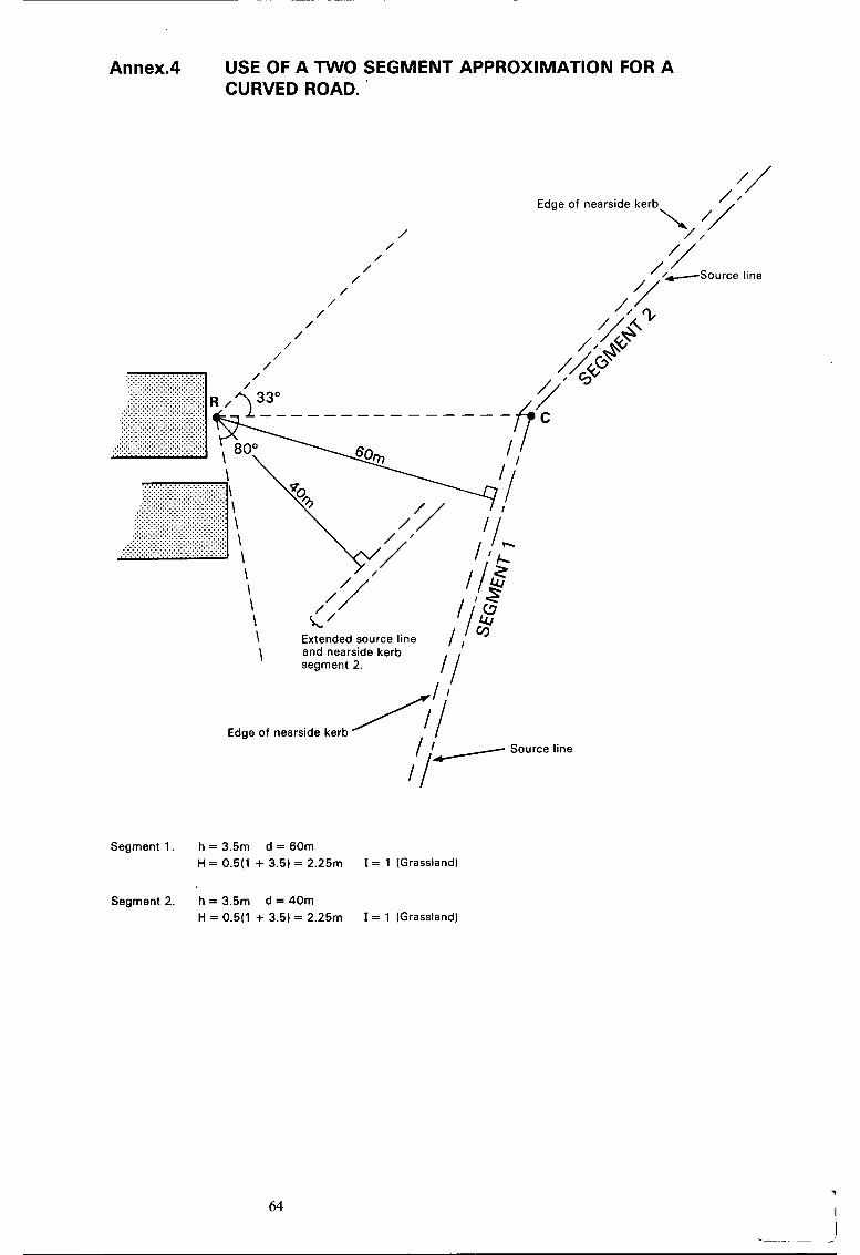
Annex.4 USE OF A TWO SEGMENT APPROXIMATION FOR A CURVED ROAD.
Edge of nearside kerb
line
Segment 1. h = 3.5m d = 60m H = 0.5(1 + 3.5) = 2.25m I = 1 (Grassland)
Segment 2. h = 3.5m d = 40m H = 0.5(1 + 3.5) = 2.25m I = 1 (Grassland)
64

ANNEX 4. USE OF A N O SEGMENT APPROXIMATION FOR A CURVED ROAD
OBJECT: To predict Llo (18-hour) value at a reception point lm from the facade and 4m above the ground.
STAGE 1. SEGMENT ROAD SCHEME: The curved road can be approximated, in this case, by two straight road segments. The segment boundary is determined by the point C where the two effective source lines intersect see diagram opposite.
STAGE 2. BASIC NOISE LEVEL: The road is subject to a speed limit of 30 mph. There is no gradient and no adjustment AV is required. The road surface is impervious and a surface correction is required as traffic speed is less than 75 km/h (para 16.1).
I SEGMENT 1 SEGMENT
1 2
Traffic flow Q vehll8-hour day
Traffic speed V km/h Heavy vehicles p %
7000
50 5
0
7000
50 5
0
Chart 3 L,c, (18-hour) dB(A)
Chart 4 correction dB(A)
Chart 6 correction dB(A)
correction dB(A)
Basic Noise Level dB(A)
Gradient G %
Road surface Impervious
STAGE 3. PROPAGATION: Propagation is unobstructed and the intervening ground cover is flat grassland. For Segment 2 the distance correction is calculated by extending the edge of the nearside carriageway (para 18).
SEGMENT SEGMENT 1
60 3.5
2.25 1
2 1
-6.7
-3.8
0
-10.5
2
-5.1
-2.9
0
-8.0
Shortest horizontal distance d m Height relative to source h m
Average height of propagation H m Absorbent ground cover I
40 3.5
2.25 1
Chart 7 correction dB(A)
Chart 8 correction dB(A)
Chart 9 correction dB(A)
Propagation Correction dB(A)
Barrier path difference 6 m
STAGE 4. SITE LAYOUT: A facade correction is required (para 26.1).
I SEGMENT SEGMENT
correction dB(A)
2
0
33
1
0
80
2 +2.5
0
-7.4
-4.9
Facade
Opposite facade angle 8’ deg.
Angle of view segment 8 deg.
reflection correction dB(A)
Chart 10 correction dB(A)
Site Layout Correction dB(A) -1.0
STAGE 5. COMBINING NOISE LEVELS: Fl -10.5
-1.0 -4.9
Basic Noise Level dB(A)
Propagation Correction dB(A)
Site Layout Correction dB(A)
Noise Contribution dB(A)
Chart 11 Combined Noise Level dB(A) 1 56.5 1 ---_-__ 54.1 J _ _ _ _ _ _ _ _ 52.7
Rounding to the nearest whole number: Predicted value of Llo (18-hour) is 57 dB(A)
65

Annex 5. EXTENDED SOURCE LINE PASSING CLOSE TO RECEPTION POINT.
For both sites A and B.
Segment 1 . h = 3.5m. d = 27.5m H = 0.5(1 + 3.5) = 2.25m I = 1 (Grassland)
Segment 2 h = 3.5m d = 10m H = 2.25 I = 1. (Grassland)
\ Source line
SEGMENT 1 - - - _ - - - - _ - - - - - - - -
Edge of /- nearside carriageway
Source line 4 I
carriageway
. - 1 - - - - -- - - -P Extended effective edge ’ of nearside carriageway
/ I of segment 2 for site B.
1 /
/ Extended effective edge of nearside carriageway of segment ,;- Extended source line segment 2.
. I -
/ for site A
/ /
The extended source line for segment 2 passes through the reception point R and precludes the use of Chart 7 (valid for d 2 4m). Two imaginary reception points A and B are chosen close to and either side of R so that this anomaly does not occur ie. at the reference distance d = 1 Om. The noise level at R is obtained by averaging the predicted values for sites A and B.
66
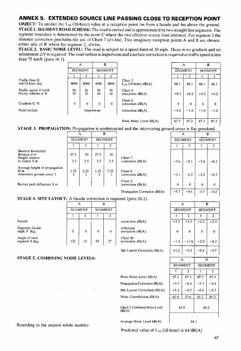
ANNEX 5. EXTENDED SOURCE LINE PASSING CLOSE TO RECEPTION POINT OBJECT: To predict the Llo (18-hour) value at a reception point lm from a facade and 4m above the ground. STAGE 1. SEGMENT ROAD SCHEME: The road is curved and is approximated by two straight line segments. The segment boundary is determined by the point C where the two effective source lines intersect. For segment 2 the distance correction precludes the use of Chart 7 (d<4m). Two imaginary reception points A and B are chosen, either side of R where for segment 2, d24m. STAGE 2. BASIC NOISE LEVEL: The road is subject to a speed limit of 30 mph. There is no gradient and no adjustment AV is required. The road surface is impervious and a surface correction is required as traffic speed is less
A
than 75 km/h (para 16.1).
B
_tB SEGMENT SEGMENT
1
61.3
-5.7
+1.2
62.8
2 1 2
61.3 61.3 67.3
-0.4 -5.1 -0.4
-9.3 -0.4 -5 .1
57.6 61.2 61.2 -------_--___________________
63.9 64.2 --------_-_-_________________
B
SEGMENT - 2
68.1
+0.2
0
-1.0
- 1
68.1
+0.2
0
-1.0
- 61.3
- 2
68.1
+0.2
0
-1.0
- 61.3
- 1
68.1
+0.2
0
-1.0
Traffic flow Q veh/18-hour day
Traffic speed V km/h Heavy vehicles p %
Chart 3 Llo (18-hour) dB(A)
Chart 4 correction dB(A)
Chart 6 correction dB(A)
correction dB(A)
Gradient G %
Road surface Impervious
Basic Noise Level dB(A) 67.3 61.3
STAGE 3. PROPAGATION: Propagation is unobstructed and the intervening ground cover is flat grassland. . - A B U SEGMENT SEGMENT SEGMENT SEGMENT -
2 -
2 -
I -
1
Shortest horizontal distance d m Height relative to source h m
27.5
3.5
2.25 1
10
3.5
2.25 1
27.5
3.5
2.25 1
10
3.5
2.25 I
Chart 7 correction dB(A)
Average height of propagation H m Absorbent ground cover I
Chart 8 correction dB(A)
Chart 9 correction dB(A)
Propagation Correction dB(A)
Barrier path difference 6 m
STAGE 4. SITE LAYOUT A facade correction is required (para 26.1). A
SEGMENT
B
SEGMENT
12 93 7, 1 1 2
+2.5 - +2.5 Facade
Opposite facade angle 0' deg.
Angle of view segment 0 deg.
correction dB(A)
reflection correction dB(A)
Chart 10 correction dB(A)
0
132
0 0
-1.3 -11.8
+1.2 -9.3 Site Layout Correction dB(A)
STAGE 5. COMBINING NOISE LEVELS:
Basic Noise Level dB(A)
Propagation Correction dB(A)
Site Layout Correction dB(A)
Noise Contribution dB(A)
Chart 11 Combined Noise Level dB(A)
Average Noise Level dB(A) Rounding to the nearest whole number:
Predicted value of Llo (18-hour) is 64 dB(A)
67
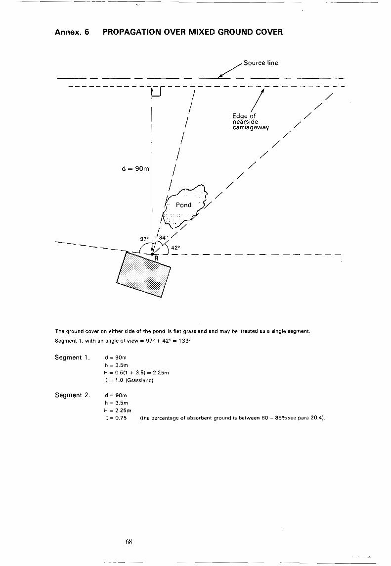
Annex. 6 PROPAGATION OVER MIXED GROUND COVER
d = 90m
I / /
/ Edge of nearside carriageway /
/ I
I
The ground cover on either side of the pond is flat grassland and may be treated as a single segment,
Segment 1, with an angle of view = 97" + 42' = 139O
Segment 1. d = 90m h = 3.5m H = 0.5(1 + 3.5) = 2.25m I = 1 .O (Grassland)
Segment 2. d = 90m h = 3.5m H = 2.25m I = 0.75 (the percentage of absorbent ground is between 60 - 89Vosee para 20.4).
68

ANNEX 6. PROPAGATION OVER MIXED GROUND COVER
OBJECT: To predict the Llo (18-hour) value at a reception point lm from a facade and 4m above the ground.
STAGE 1. SEGMENT ROAD SCHEME: Most of the intervening ground cover is grassland and therefore absorbent while the pond is designated as non-absorbent, para 20.1. The angle of the view subtended by the pond at the reception point defines the boundary of segment 2. The area either side of segment 2 can be treated together by combining their angles of view to form segment 1 (paras 20.3 and 20.4).
STAGE 2. BASIC NOISE LEVEL: The road is a single carriageway subject to a speed limit of 50 mph. There is no gradient and no adjustment AV is required. The road surface is impervious and a surface correction is required as traffic speed is less than 75 km/h (para 16.1).
Traffic flow Q veh/l8-hour day
Traffic speed V km/h Heavy vehicles p %
Gradient G %
Road surface
SEGMENT
1
20000
70 15
0
- 2
2000c
70 15
-
0
Impervious
Chart 3 L,,, (18-hour) dB(A)
Chart 4 correction dB(A)
Chart 6 correction dB(A)
correction dB(A)
Basic Noise Level dB(A)
SEGMENT
1
72.1
+2.6
0
-1.0
73.7
2
72.1
+2.6
0
-1.0
73.7
STAGE 3. PROP. .GATION: Propagation is unc,,.ructec. .md the intervening ground cover is flat. For Segment 2 it is estimated that the percentage of absorbent ground is between 60-89% and a value of I = 0.75 is used. (para 20.4).
Shortest horizontal distance d m Height relative to source h m
Average height of propagation H m Absorbent ground cover I
Barrier path difference 6 m
SEGMENT
1
90 3.5
2.25 1
2
90 3.5
2.25 0.75
Chart 7 correction dB(A)
Chart 8 correction dB(A)
Chart 9 correction dB(A)
Propagation Correction dB(A)
STAGE 4. SITE LAYOUT: A facade correction is required (para 26.1). SEGMENT
correction dB(A)
reflection correction dB(A)
Chart 10 139 34 correction dB(A)
Site Layout Correction dB(A)
Facade
Opposite facade angle 8’ deg.
Angle of view segment 0 deg.
STAGE 5. COMBINING NOISE LEVELS:
Rounding to the nearest whole number:
Basic Noise Level dB(A)
Propagation Correction dB(A)
Site Layout Correction dB(A)
Noise Contribution dB(A)
Chart 11 Combined Noise Level dB(A)
SEGMENT
1
-8.4
-4.6
0
-13.0
2
-8.4
-3.5
0
-11.9
I SEGMENT
SEGMENT
62.1
63.3
Predicted value of Llo (18-hour) is 63 dB(A)
69

Annex. 7 ELEVATED ROAD WITH GRASS BANKS.
PLAN OF SITE
Source line C-l
- - A S - / - I I I
- - - - - - - - - - _ - - _ - - - - _ - -
Edge of nearside carriageway / /
/ /
/ /
/ /
U
/ /
/ /
/
\
\ \ \ \ \ \ \ \ \ \
R $eception point I I
C ’ d
CROSS-SECTION OF SITE CC:
3.5m 2.5m 7.5m 50m
CONDITION 1: d = 60m h = 4 - 3.5 = 0.5m
H = 2 6(0.5 + 0.5) 63.5 ( 2
= 3.29m
I = 1 (Grassland)
CONDITION 2:
7.5 (0.5 + 3.5) + 50(3.5 + 3.5) 0.5 + 2 2 )+T
Path difference = SB + BR - SR
= (0.5’+ 6’) !5 + (1’+ 57.5*)
= 0.028m
- (0.5’+ 63.5’1%
70
.

ANNEX 7. ELEVATED ROAD WITH GRASS BANKS
OBJECT: To predict the Llo (18-hour) value prior to the development of residential houses. A reception point is chosen lm from the most exposed part of the proposed eligible facade and is 4m above the ground (para 8).
STAGE 1. SEGMENT ROAD SCHEME: The site is open with no changes in traffic variables or propagation conditions. The road can therefore be treated as a single segment.
STAGE 2. BASIC NOISE LEVEL: The road is classified as a dual carriageway with a speed limit of 50 mph. There is no gradient and no adjustment AV is required. The road surface is impervious and a surface correction is not required as traffic speed is greater than 75 km/h (para 16). Traffic flow Q veh/lS-hour day
Traffic speed V km/h Heavy vehicles p %
Gradient G %
Road surface
35000
80 10
0
Impervious
Chart 3 Llu (18-hour) dB(A)
Chart 4 correction dB(A)
Chart 6 correction dB(A)
correction dB(A)
Basic Noise Level dB(A)
74.5
+2.6
0
0
77.1
STAGE 3. PROPAGATION: The road is elevated on a grass embankment. The view of the source line is unobstructed but the propagation path passes close to the edge of the embankment. The intervening ground cover is absorbent. The propagation correction is therefore calculated assuming ground attenuation (Condition 1) or that the embankment provides screening with the reception point in the illuminated zone (Condition 2), para 22.3.
Shortest horizontal distance d m Height relative to source h m
Average height of propagation H m Absorbent ground cover I
Barrier path difference 6 m
CONDITION I
60 0.5
3.29 1
2
60 0.5
0.028
Chart 7 correction dB(A)
Chart 8 correction dB(A)
Chart 9 correction dB(A)
Propagation Correction dB(A)
CONDITION
0 -2.4
-9.5 -9.1
STAGE 4. SITE LAYOUT: Since residential development is planned a correction for the facade will normally be required (para 26.1).
Facade
Opposite facade angle €I' deg.
Angle of view segment 8 deg.
CONDITION
1
0
122
2
0
122
correction dB(A)
reflection correction dB(A)
Chart 10 correction dB(A)
Site Layout Correction dB(A)
CONDITION
1
+2.5
0
-1.7
+0.8
2
+2.5
0
-1.7
+0.8
STAGE 5. COMPARING NOISE LEVELS: I CONDITION I
Basic Noise Level dB(A)
Propagation Correction dB(A)
Site Layout Correction dB(A)
Noise Level dB(A) 68.4
The level redicted assuming the edge of the embankment acts as a barrier is higher than the level predicted assumingground attenuation. The lower of tge two noise levels is adopted for prediction purposes, giving a value of 68.4 db(A).
Rounding to the nearest whole number gives: Predicted value of Ll0 (18-hour) is 68 dB(A)
71

Annex. 8 ROAD W T H PURPOSE - BUILT NOISE BARRIER
PLAN OF SITE
C 9 Source line Edge of nearside carriageway I
- !S - - - - - _ _ - - - - - - - - _ _ - _ _ _
Noise barrier \ f ‘\ \ Safety \
\ \ fence \ \ \ \ \ \ \
SECT1 0 N
\ \
\ \ \
\ \
\
\ \ \
\ \
THROUGH CC‘
E d II ‘c
6
/ /
/ /
/ \ \
R I Reception point
/ /
/ /
/ /
/ /
/ 0
/ /
0 0
0 0
0 0
/ /
R
Noise barrier path difference, 6 = SB + BR - SR
= (2.5’+ 8.5’)’’ + (1’+ 37’)+ - (3.5’+ 45.5’)$
= 0 .239m
Safety fence path difference < 0.001 m
72

ANNEX 8. ROAD WITH PURPOSE-BUILT NOISE BARRIER OBJECT: To predict the Llo (18-hour) value 1 m from the rear facade of a dwelling. Reception point is4m above the ground. STAGE 1. SEGMENT ROAD SCHEME: Propagation is obstructed by a noise barrier which defines the boundaries of segment 1. A safety fence also runs along the whole length of the road. The segments either side of segment 1 can be treated as a single segment by combining their angles of view subtended at the reception point to form segment 2. The remainder of the site is effectively shielded by houses and may be ignored.
STAGE 2. BASIC NOISE LEVEL: Although the road is on a gradient no adjustment AV is required as the traffic speed is measured. A surface correction is not required as traffic speed is greater than 75 km/h (para 16).
SEGMENT I SEGMENT
+0.9
Traffic flow Q veh/Whour day
Traffic speed V kmlh Heavy vehicles p %
Chart 3 Llo (18-hour) dB(A)
Chart 4 correction dB(A)
Chart 6 correction dB(A)
correction dB(A)
Basic Noise Level dB(A)
6300 I 6300
91 12
91 12
Gradient G %
Road surface
3 1 3
Impervious
STAGE 3. PROPAGATION: Segment 1 consists effectively of two barriers (para 22.4) but the screening due to the safety fence is small compared with the noise barrier and may be ignored. For segment 2 the screening due to the safety fence is assumed greater than that offered by ground absorption (para 22.3). All path differences are calculated in the same vertical plane as the distance correction (para 21).
I SEGMENT SEGMENT
2
42 3.5
c.001
1
-5.3
0
-11.2
- 16.5
2 Shortest horizontal distance d m Height relative to source h m 3.5
Average height of propagation H m Absorbent ground cover I
Barrier path difference 6 m 1 0.239
Chart 7 correction dB(A)
Chart 8 correction dB(A)
Chart 9 correction dB(A)
Propagation Correction dB(A)
-5.3
0
-5.0
- 10.3
STAGE 4. SITE LAYOUT: A facade correction is required (para 26.1). SEGMENT I SEGMENT 7 -4.6
1 1 2
Facade
Opposite facade angle 0’ deg.
Angle of view segment 0 deg.
correction dB(A) +2.5
0
-3.3
-0.8
0
84
0
35
reflection correction dB(A)
Chart 10 correction dB(A)
Site Layout Correction dB(A)
STAGE 5. COMBINING NOISE LEVELS:
Basic Noise Level dB(A)
Propagation Correction dB(A)
Site Layout Correction dB(A)
Noise Contribution dB(A)
Chart 11 Combined Noise Level dB(A) I 59.0
Rounding to the nearest whole number: Predicted value of Llo (18-hour) is 59 dB(A)

Annex 9. CURVED ROAD WITH PURPOSE-BUILT NOISE BARRIER
/ so ke
E Noise barrier
Edge of nearside / barrier,
segment 1 . carriageway Segment 1. \ 8
/ \ ,
\ \ / Extended
urce line, rb and
Extended source line, kerb and barrier, segment 2. ----- ---- - --- - - - - -
Segment 1. Cross-section through RS,
R
- I
=;- Extended equivalent barrier *I
0.5m : +I 45m I-
Path difference= S,B,+B,R-S,R
= (2.5’+ 1 € 1 . 5 ~ ) ’ ~ + (12+45’)%- (3.5‘+ 63.5’)’’
= 0.083m.
Segment 2. Cross section through RS,
Path difference = S,B,+B,R-S,R
= (2.5’+ 18.52)k+ (12+ 77’)4 - (3.5’+ 95.5’).5
= 0.1 1 1 m.
74
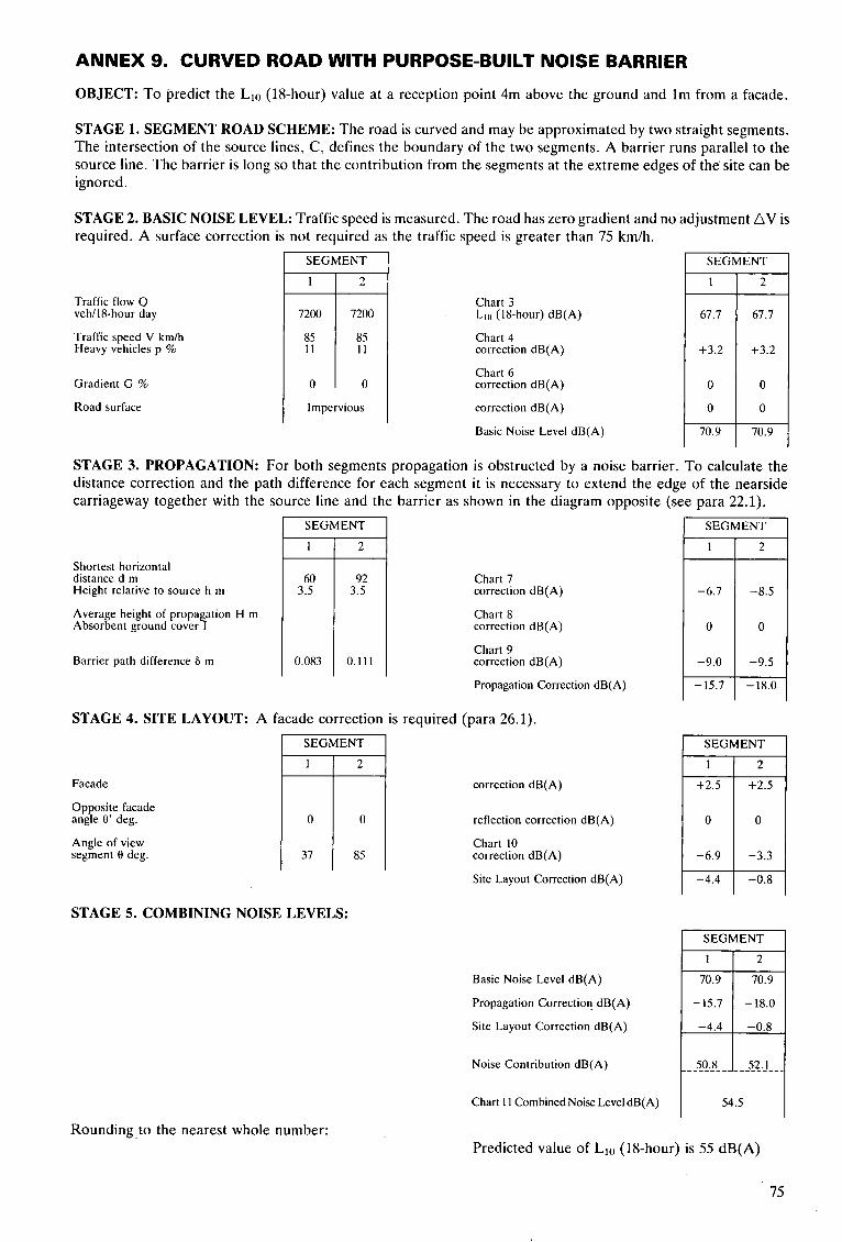
ANNEX 9. CURVED ROAD WITH PURPOSE-BUILT NOISE BARRIER
OBJECT: To predict the Ll0 (18-hour) value at a reception point 4m above the ground and lm from a facade.
STAGE 1. SEGMENT ROAD SCHEME: The road is curved and may be approximated by two straight segments. The intersection of the source lines, C, defines the boundary of the two segments. A barrier runs parallel to the source line. The barrier is long so that the contribution from the segments at the extreme edges of the site can be ignored.
STAGE 2. BASIC NOISE LEVEL: Traffic speed is measured. The road has zero gradient and no adjustment AV is required. A surface correction is not required as the traffic speed is greater than 75 km/h.
I SEGMENT SEGMENT
1
7200
85 11
0
2
7200
85 11
0
2
67.7
+3.2
0
0
70.9
Chart 3 L,,, (18-hour) dB(A)
Traffic flow Q vehll8-hour day
Traffic speed V km/h Heavy vehicles p %
Chart 4 correction dB(A)
Chart 6 correction dB(A)
1 +3.2
I 0 Gradient G %
Road surface l 0 correction dB(A) Impervious
Basic Noise Level dB(A) p- STAGE 3. PROPAGATION: For both segments propagation is obstructed by a noise barrier. To calculate the distance correction and the path difference for each segment it is necessary to extend the edge of the nearside carriageway together with the source line and the barrier as shown in the diagram opposite (see para 22.1).
SEGMENT SEGMENT
1 1 2 2 1
T 0.083 0.111
Shortest horizontal distance d m Height relative to source h m
Average height of propagation H m Absorbent ground cover I
Chart 7 correction dB(A)
Chart 8 correction dB(A)
-6.7
0
-9.0
-15.7
-8.5
0
-9.5
-18.0
Chart 9 correction dB(A) Barrier path difference 6 m
Propagation Correction dB(A)
STAGE 4. SITE LAYOUT: A facade correction is required (para 26.1).
I SEGMENT SEGMENT
-4.4
1 2 2
+2.5
0
-3.3
-0.8
Facade
Opposite facade angle 8’ deg.
Angle of view segment 0 deg.
correction dB(A)
0
37
0
85
reflection correction dB(A)
Chart 10 correction dB(A)
Site Layout Correction dB(A)
STAGE 5. COMBINING NOISE LEVELS:
I SEGMENT
-15.7 -18.0
-4.4 -0.8
50.8 _ _ _ _ _ _ _ _
Basic Noise Level dB(A)
Propagation Correction dB(A)
Site Layout Correction dB(A)
Noise Contribution dB(A)
Chart 11 Combined Noise Level dB(A) I 54.5
Predicted value of Ll0 (18-hour) is 55 dB(A) Rounding to the nearest whole number:
75

Annex 10. SCREENING DUE TO NOISE BARRIER WHICH IS NOT PARALLEL TO THE ROAD.
- - S - -e
RO bisects the angle of view of the barrier
-- _ - - - c--
Cross-Section through SR.
R ;;. Extended equivalent barrier ... ... ... ... ... . . . ... ... .... ... .... ... .... . . . .... .... ..... .... ..... ..... .....
* -- /-- ...
.. . . . ..... ..... ..... ...... ..... ...... . . . . . ...... ...... ...... ...... ...... ...... ...... ...... I I
I
-/---
I-
I /
! E
1-1-14
/ /
Im S -’- 0.5m
3.5m 20m 60m
The path difference is calculated by extending the equivalent barrier Z,Z, to B which lies in the vertical plane through SR, such that
path difference (6) = SB + BR - SR 1
= (2.5’+ 23.5’1% + (1 + (3.5’+ 83.5’)\
= 0.0681~1
76
. J

L a
ANNEX 10. SCREENING DUE TO NOISE BARRIER WHICH IS NOT PARALLEL TO THE ROAD OBJECT: To predict the L ~ o (18-hour) value 1m from a facade and 4m above the ground. STAGE 1. SEGMENT ROAD SCHEME: Propagation is obstructed by a noise barrier which defines the boundaries of segment 1. The barrier is not parallel to the source line. A preliminary investigation reveals that the variation of barrier potential calculated for equivalent barriers parallel to the source at various points along the length of the barrier differs by less than 2 dB(A) and therefore further subdivision is not necessary (para 11). Segment 2 consists of the remaining segments where propagation is unobstructed. STAGE 2. BASIC NOISE LEVEL: Traffic speed is measured. The road has zero gradient and no adjustment AV is required. A surface correction is not required as the traffic speed is greater than 75 km/h.
SEGMENT I SEGMENT I r 82.6 ! 82.6
1 2
Traffic flow Q vehll8-hour day
Traffic speed V km/h Heavy vehicles p %
Chart 3 Llo (18-hour) dB(A)
Chart 4 correction dB(A)
Chart 6 correction dB(A)
Correction dB(A)
Basic Noise Level dB(A)
50000
100 30
0
50000
100 30
0 Gradient G %
Road surface Impervious
STAGE 3. PROPAGATION: For segment 1 the barrier is rotated parallel to the source line about the bisector of the segment angle and extended so that the path difference is calculated in the same vertical plane as the distance correction (para 22.2). The intervening ground cover is grassland and flat.
SEGMENT SEGMENT
1
-7.9
0
-8.7
2
-7.9
-4.4
0
- 12.3
Shortest horizontal distance d m Height relative to source h m
Average height of propagation H m Absorbent ground cover I
Chart 7 correction dB(A)
Chart 8 correction dB(A)
Chart 9 correction dB(A)
Propagation Correction dB(A)
2.25
0.068 Barrier path difference 6 m
-16.6
STAGE 4. SITE LAYOUT: A facade correction is required (para 26.1). SEGMENT SEGMENT
zfz 2 1
0
25
Facade
Opposite facade angle 0’ deg.
Angle of view segment 0 deg.
correction dB(A)
0
125
reflection correction dB(A)
Chart 10 correction dB(A)
Site Layout Correction dB(A)
0
-8.6
0
-1.6
STAGE 5. COMBINING NOISE LEVELS: SEGMENT
71.2
71.5
Basic Noise Level dB(A)
Propagation Correction dB(A)
Site Layout Correction dB(A)
Noise Contribution dB(A)
Chart 11 Combined Noise Level dB(A)
Rounding to the nearest whole number: Predicted value of LIO (18-hour) is 72 dB(A)
77

Annex 11. ROAD SCREENED BY W O NOISE BARRIERS
- SEGMENT 1
- I / t Barrier 1 / B,
I + SEGMENT 2 - SEGMENT 3 /
\ -- ---- ...... ...... ................. ................ ................. ................ ................. ................ ................. ................ . . . . . . . . . . . . . . .
......
Barrier 2 extended to cut SR at 8 2
d = 6 0 m
Cross-Section through SR.
Extended equivalent barrier
I / / I /
/ / 1 /
15m 42.5 m Iu1-1- 3.5m 2.5m
Barrier 1. Path difference = SB, + B, R - SR
= (1.5’+ 6’)’z + (2’+ 57.5’1’2 - (3.5’+ 63.5’)%
= 0.1 23m
Barrier 2. The barrier is extended to meet the vertical plane through SR at B, Path difference = SB,+ B,R - SR.
= (2.5’+ 212)$ + (1 + 42.5’)k - (3.5’+ 63.5’)+
= 0.064m.
78

ANNEX 11. ROAD SCREENING BY TWO NOISE BARRIERS OBJECT: To predict the Llo (18-hour) value at a reception point l m from a facade and 4m above the ground.
STAGE 1. SEGMENT ROAD SCHEME: As the degree of screening varies along the road length the road scheme is segmented at each point along the source line where the screening changes with respect to the position of the reception point, see figure opposite. Both barriers extend off the plan. At the extreme edges of the site further screening is provided by houses and the contribution to the overall noise level from these segments is negligible.
STAGE 2. BASIC NOISE LEVEL: The road is a singlecarriageway subject to a speed limit of 50 mph. There is no gradient and no adjustment AV is required. The road surface is impervious and a surface correction is required as traffic is less than 75 km/h (para 16.1).
SEGMENT SEGMENT
2
66.1
+1.8
0
-1.0
66.9
3
66.1
+1.8
0
-1.0
66.9
1
66.1
+1.8
0
-1.0
66.9
2 3 1
Traffic flow Q veh/lS-hour day
Traffic speed V km/h Heavy vehicles p %
Chart 3 Llo (18-hour) dB(A) 5000
70 10
0
5000
70 10
0
5000
70 10
0
Chart 4 correction dB(A)
Chart 6 correction dB(A)
correction dB(A)
Basic Noise Level dB(A)
Gradient G %
Road surface ipervious
STAGE 3. PROPAGATION: For all segments the propagation is obstructed by noise barriers. For segment 2 both barriers provide screening and the potential barrier correction is calculated in accordance with para 35 where: AA = -9.7 dB(A); AB = -8.6 dB(A); M = 15m; d = 60m; and J = 0.7.
I SEGMENT SEGMENT
T 0. I23
2 3 3 1
-6.7
0
-9.7
0
- 16.4
Shortest horizontal distance d m Height relative to source h m
Average height of propagation H m Absorbent ground cover I
60 3.5
0.064
Chart I correction dB(A)
Chart 8 correction dB(A)
Chart 9 correction dB(A)
para 35 correction dB(A)
Propagation Correction dB(A)
-6.&
0
0
-10.9
-6.1
0
-8.6
0
Barrier path difference 6 m
Distance between barriers M m I I 5 -17.6 -15.3
STAGE 4. SITE LAYOUT: A facade correction is required (para 26.1). SEGMENT SEGMENT I
2 +2.5
0
-6.6
3
+2.5
0
-8.4
3
Facade
Opposite facade angle 8’ deg.
Angle of view segment tl deg.
correction dB(A)
0
26
reflection correction dB(A)
Chart 10 correction dB(A)
Site Layout Correction dB(A)
100 39
-4.1 -5.9
STAGE 5. COMBINING NOISE LEVELS: SEGMENT
Basic Noise Level dB(A)
Propagation Correction dB(A)
Site Layout Correction dB(A)
-16.4 -17.6 -15.3
-0.1 -4.1 -5.9
45.2 _ _ _ _ _ _ _ _ _ _ _ _ _ _ _ _ _ _ _ _ _ _ _ Noise Contributions dB(A)
Chart 11 Combincd Noise Level dB(A)
52.6
Rounding to the nearest whole number gives: Predicted value of LIO (18-hour) is 53 dB(A)
79
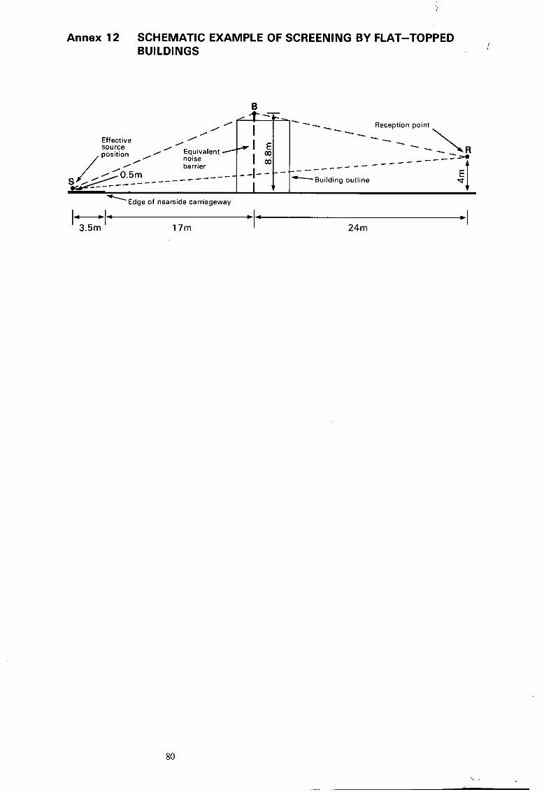
Annex 12 SCHEMATIC EXAMPLE OF SCREENING BY FLAT-TOPPED BUILDINGS
B
. 0 Of?T= Effective
barrier
- *I -Building outline
Edge of nearside carriageway -. w -
3.5m 17m 24m
80

ANNEX 12. SCHEMATIC EXAMPLE OF SCREENING BY FLAT-TOPPED BUILDINGS
OBJECT: To predict the potential barrier correction for an &metre high flat-topped building erected 15m from the nearside kerb. Note that this procedure is not usually required when evaluating ridged buildings as the ridge itself will generally define the equivalent barrier configuration.
PROCEDURE: (i) On a scaled cross-section draw a line from the effective source position S (3.5m in from the edge of the nearside kerb and 0.5m high) to pass through the near top edge of the building.
(ii) Draw a line from the reception point R (4m above the ground and 41m from the edge of the kerb) through the other top edge of the building and extend this to intersect the above line at B.
(iii) Scale off the height and position of the equivalent barrier from the intersection point B of the above two lines.
In the example given the effective height of the equivalent barrier is estimated to be 8.8m and the effective position of the equivalent barrier is 17m from the edge of the nearside kerb.
Having determined the equivalent barrier configuration it will, in general, still be necessary to calculate the path difference rather than to use graphical evaluation as the latter method is likely to lead to significant error (the path difference is the difference between two relatively large numbers).
For this example:
path difference = SB + BR - SR = (8.3’ + 20.5’) ’’’ + (4.8’ + 24’)”’ -(3.5’ + 44.5’)’” = 1.954m
Chart 9. Potential barrier correction = -18.1 dB(A)
The remainder of the prediction procedures are illustrated by various other examples in these Annexes.
81

Annex 13. SIDE ROAD LEADING OFF A MAJOR ROAD WITH HOUSES FLANKING MAJOR ROAD.
I I
I I
I I
I
Edge of nearside carriageway
I / I I
Reception point . f
E
II (I)
U
/ I
Total angle of view of opposite facades = 6O+ 9'= 15' 15 The reflection correction due to opposite facades = - x 1.5 = 0.9 dB(A) 25
82
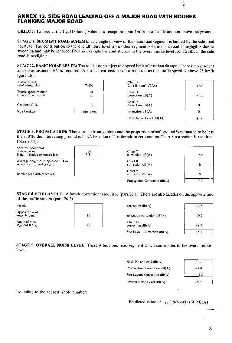
ANNEX 13. SIDE ROAD LEADING OFF A MAJOR ROAD WITH HOUSES FLANKING MAJOR ROAD
OBJECT: To predict the LIO (18-hour) value at a reception point lm from a facade and 4m above the ground.
STAGE 1. SEGMENT ROAD SCHEME: The angle of view of the main road segment is limited by the side road aperture. The contribution to the overall noise level from other segments of the main road is negligible due to screening and may be ignored. For this example the contribution to the overall noise level from traffic in the side road is negligible.
STAGE 2. BASIC NOISE LEVEL: The road is not subject to a speed limit of less than 60 mph. There is no gradient and no adjustment AV is required. A surface correction is not required as the traffic speed is above 75 km/h (para 16). Traffic flow Q veh/lS-hour day
Traffic speed V km/h Heavy vehicles p %
Gradient G %
Road surface
70000
81 20
0
Impervious
Chart 3 L,,, (18-hour) dB(A)
Chart 4 correction dB(A)
Chart 6 correction dB(A)
correction dB(A)
Basic Noise Level dB(A) U 81.7
STAGE 3. PROPAGATION: There are no front gardens and the proportion of soft ground is estimated to be less than 10%, the intervening ground is flat. The value of I is therefore zero and no Chart 8 correction is required (para 20.4). Shortest horizontal distance d m Height relative to source h m
Average height of propagation H m Absorbent ground cover I
Barrier path difference 6 m
64 3.5
Chart 7 correction dB(A)
Chart 8 correction dB(A)
Chart 9 correction dB(A)
Propagation Correction dB(A) I STAGE 4. SITE LAYOUT: A facade correction is required (para 26.1). There are also facades on the opposite side of the traffic stream (para 26.2).
I Facade
Opposite facade angle 8' deg.
Angle of view segment 8 deg
I l5
I 25
correction dB(A)
reflection correction dB(A)
Chart 10 correction dB(A)
Site Layout Correction dB(A)
STAGE 5. OVERALL NOISE LEVEL: There is only one road segment which contributes to the overall noise level.
1p Basic Noise Level dB(A)
Propagation Correction dB(A)
Site Layout Correction dB(A)
Overall Noise Level dB(A) I 69.5
Rounding to the nearest whole number:
Predicted value of Llo (18-hour) is 70 dB(A)
c_
83

Annex 14 LOW TRAFFIC FLOW ROAD AFTER THE OPENING OF A BY-PASS
Effective source line
- - J - Edge of nearside carriageway
----- _ _ _ _ _ _ _ _ _ d=4m
0 Reception point
84
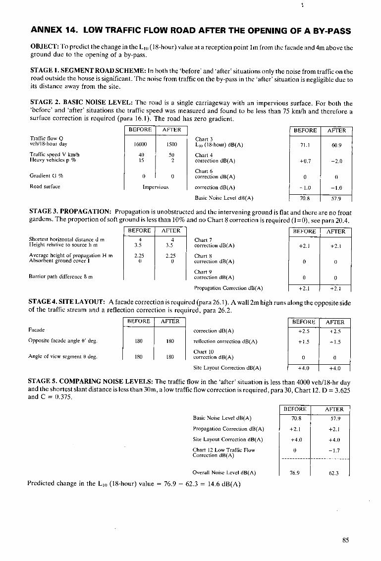
ANNEX 14. LOW TRAFFIC FLOW ROAD AFTER THE OPENING OF A BY-PASS
71.1
+0.7
OBJECT: To predict the change in the Llo (18-hour) value at a reception point l m from the facade and 4m above the ground due to the opening of a by-pass.
~~
60.9
-2.0
STAGE 1. SEGMENT ROAD SCHEME: In both the ‘before’ and ‘after’ situations only the noise from traffic on the road outside the house is significant. The noise from traffic on the by-pass in the ‘after’ situation is negligible due to its distance away from the site.
Site Layout Correction dB(A)
STAGE 2. BASIC NOISE LEVEL: The road is a single carriageway with an impervious surface. For both the ‘before’ and ‘after’ situations the traffic speed was measured and found to be less than 75 km/h and therefore a surface correction is required (para 16.1). The road has zero gradient.
+4.0 I +4.0
Traffic flow Q veh/l8-hour day
Traffic speed V km/h Heavy vehicles p %
Gradient G %
Road surface
I6000
Impervious
Chart 3 Llo (18-hour) dB(A)
Chart 4 correction dB(A)
Chart 6 correction dB(A)
correction dB(A)
Basic Noise Level dB(A)
BEFORE I AFTER
O I 0
STAGE 3. PROPAGATION: Propagation is unobstructed and the intervening ground is flat and there are no front gardens. The proportion of soft ground is less than 10% and no Chart 8 correction is required (I=O), see para 20.4.
Chart 7 correction dB(A)
correction dB(A) 2.25 2.25 Chart 8
Shortest horizontal distance d m Height relative to source h m
Average height of propagation H m Absorbent ground cover I
Barrier path difference 8 m Chart 9 correction dB(A)
Propagation Correction dB(A)
STAGE 4. SITE LAYOUT: A facade correction is required (para 26.1). A wall 2m high runs along the opposite side of the traffic stream and a reflection correction is required, para 26.2.
Facade
Opposite facade angle 8’ deg.
Angle of view segment 8 deg.
correction dB(A)
I BEFORE 1 A F T E R 1
I 180 1 180 I rcflection correction dB(A) I +IS I +IS I I Chart 10 I 180 I 180 correction dB(A)
STAGE 5. COMPARING NOISE LEVELS: The traffic flow in the ‘after’ situation is less than 4000 veh/l&hr day and the shortest slant distance is less than 30m, a low traffic flow correction is required, para 30, Chart 12. D = 3.625 and C = 0.375.
Basic Noise Level dB(A)
Propagation Correction dB(A)
Site Layout Correction dB(A)
Chart 12 Low Traffic Flow Correction dB(A)
Overall Noise Level dB(A)
Predicted change in the LIO (18-hour) value = 76.9 - 62.3 = 14.6 dB(A)
BEFORE
70.8
+2.1
+4.0
0
76.9
AFTER
57.9
+2.1
+4.0
-1.7 _ _ _ _ _ _ _ _ _ _ _ _ _
62.3
85

Annex 15. END OF SCHEME
EXIST1 NG SITUATION
R Reception point 4
FUTURE SITUATION
-e------- --- l-hJ 35"
Old Segment -
Physical end of scheme / Source line
I Improved Segment
N.B. The central reservation for the improved segment is less than 5m wide and therefore both carriageways are considered to act as a single road and are treated in the calculation as a single segment.
86
~
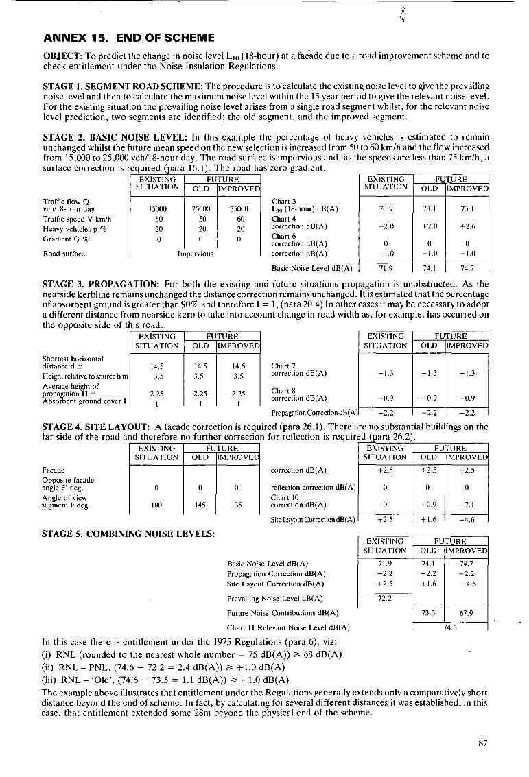
G 'b
Traffic speed V km/h
Gradient G % Heavy vehicles p %
ANNEX 15. END OF SCHEME OBJECT: To predict the change in noise level Llo (18-hour) at a facade due to a road improvement scheme and to check entitlement under the Noise Insulation Regulations.
50 50 60 20 20 20 0 0 0
STAGE 1. SEGMENT ROAD SCHEME: The procedure is to calculate the existing noise level to give the prevailing noise level and then to calculate the maximum noise level within the 15 year period to give the relevant noise level. For the existing situation the prevailing noise level arises from a single road segment whilst, for the relevant noise level prediction, two segments are identified; the old segment, and the improved segment.
EXISTING SITUATION
STAGE 2. BASIC NOISE LEVEL: In this example the percentage of heavy vehicles is estimated to remain unchanged whilst the future mean speed on the new selection is increased from 50 to 60 km/h and the flow increased from 15,000 to 25,000 veh/l&hour day. The road surface is impervious and, as the speeds are less than 75 km/h. a surface correction is reauired fDara 16.1). The road has zero gradient.
FUTURE OLD IMPROVED
EXISTING FUTURE
15000 Traffic flow Q veh/lS-hour day
EXISTING SITUATION
Chart 3 Llo (18-hour) dB(A) Chart 4
Chart 6 correction dB(A) +2.0
correction dB(A) 0 correction dB(A) -1.0
Basic Noise Level dB(A) 171.9 STAGE 3. PROPAGATION: For both the existing and future situations propagation is unobstructed. As the nearside kerbline remains unchanged the distance correction remains unchanged. It is estimated that the percentage of absorbent ground is greater than 90% and therefore I = 1, (para 20.4) In other cases it may be necessary to adopt a different distance from nearside kerb to take into account change in road width as, for example, has occurred on the opposite side of this road. _ _
EXISTING FUTURE
Shortest horizontal distance d m Height relative to source h m
Chart 7 correction dB(A)
EXISTING FUTURE SITUATION OLD IMPROVED
I -1.3 I -1.3 I -1.3
.25 I 2.25 I L''d'L I -0.9 I -0.9 I -0.9 I & ' - 'B(A) I I
Propagation Correction dB(Aj -2.2 I -2.2 I -2.2
STAGE 4. SITE LAYOUT: A facade correction is required (para 26.1). There are no substantial buildings on the far side of the road and therefore no further correction for reflection is required (para 26.2).
EXISTING FUTURE SITUATION OLD I I M P R O V E D
Facade Opposite facade angle 0' deg. Angle of view segment 0 deg.
I I I I correction dB(A)
reflection correction dB(A) Chart 10 correction dB(A)
Site Layout Correction dB(A)
STAGE 5. COMBINING NOISE LEVELS:
Basic Noise Level dB(A) Propagation Correction dB(A) Site Layout Correction dB(A)
Prevailing Noise Level dB(A)
Future Noise Contributions dB(A)
Chart 1 1 Relevant Noise Level dB(A)
In this case there is entitlement under the 1975 Regulations (para 6), viz: (i) RNL (rounded to the nearest whole number = 75 dB(A)) > 68 dB(A) (ii) RNL - PNL, (74.6 - 72.2 = 2.4 dB(A)) 3 +1.0 dB(A) (iii) RNL - 'Old', (74.6 - 73.5 = 1.1 dB(A)) 3 +1.0 dB(A)
-0.9 -7.1
+2.5 +1.6 -4.6
EXISTING
-2.2 -2.2 +2.5 +1.6
'URE MPROVEt
74.7 -2.2 -4.6
67.9
1.6
The example above illustrates that entitlement under the Regulations generally extends only a comparatively short distance beyond the end of scheme. In fact, by calculating for several different distances it was established, in this case, that entitlement extended some 28m beyond the physical end of the scheme.
87
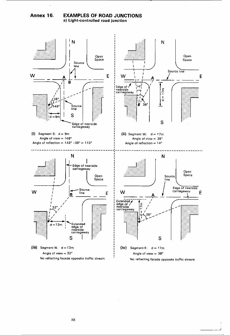
Annex 16. EXAMPLES OF ROAD JUNCTIONS a) Light-controlled road junction
I
carriageway
(i) Segment S: d = 9m : (ii) Segment W: d = 17m Angle of view = 38"
Angle of reflection = 148" -38" = 1 10" Angle of reflection = 14'
. . . . . . . . . . . . . . . . . . . . . . . . . . . . . . . . . . . . . . . . . . . . . . . .8. . . . . .*. . . . . . . . . . .*. . . . . . . . . . . . . . . . . . . . . , . . . . . . . . . .
Angle of view = 148"
N N
I /Source
I - -- I l e line E w 7 /
/ I
I / /
d = 1 3 m I I
line
Edge of nearside
E A 1 carriageway -A- w I- --
R 4 0
0 0
S
/
(iii) Segment N: d = 13m : ( iV) Segment E: d = 17m
Angle of view = 38" Angle of view = 32"
No reflecting facade opposite traffic stream '
No reflecting facade opposite traffic stream
88

ANNEX 16. EXAMPLES OF ROAD JUNCTIONS. (a) A light-controlled road junction. OBJECT: To predict the value of Llo (18-hour) at a reception point l m from a facade and 4m above ground in the vicinity of a light-controlled road junction.
STAGE 1. SEGMENT ROAD SCHEME: In this example, the effective source lines for junction arms S and N are extended to intersect the source line WE at A and B respectively. Each arm of the junction is then treated as a separate segment as illustrated. NB Point A is chosen as the boundary between the W and E segments rather than B as this leads to a marginally higher overall noise level (see para 33) . For this example the contribution to the overall noise level from road segments screened by buildings is assumed negligible.
STAGE 2. BASIC NOISE LEVEL: In the region of the junction the estimated speed for traffic on that class of road is adopted rather than the actual speed of traffic crossing the junction. As the estimated traffic speed is less than 75
S
72.1
+1.9
0 -1.0
73.0
km/h a surface correction is required (para 16.1). SEGMENT
W N E
69.9 69.1 71.7
+1.4 +0.2 +1.9
0 0 0 -1.0 -1.0 -1.0
70.3 68.3 72.6
Traffic flow Q veh/lS-hour day Traffic speed V km/h Heavy vehicles p %
SEGMENT
S W N E
Shortest horizontal distance d m 9 17 13 17 Chart 7
Average height of propagation H m Chart 8
Chart 9
Height relative to source h m 3.5 3.5 3.5 3.5 correction dB(A)
Absorbent ground cover I
Barrier path difference 6 m
correction dB(A)
correction dB(A)
Propagation Correction dB(A)
ml 20000 12000 10000 18000
SEGMENT
S W N E
+0.2 -1.9 -1.0 -1.9
0 0 0 0
0 0 0 0
+0.2 -1.9 - 1.0 - 1.9
Impervious Gradient G % Road surface
Basic Noise Level dB(A) Propagation Correction dB(A) Site Layout Correction dB(A)
Noise Contribution dB(A)
Chart 11 Combined Noise Level dB(A)
Chart 3 Llo (18-hour) dB(A) Chart 4 correction dB(A) Chart 6 correction dB(A) correction dB(A)
Basic Noise Level dB(A)
SEGMENT
S W N E
73.0 70.3 68.3 72.6 +0.2 -1.9 - 1 .O -1.9 +2.7 -3.7 -5.0 -4.3
75.9 64.7 62.3 66.4 ---_-__-__-__-__--_-------__--
76.8
SEGMENT
STAGE 4. SITE LAYOUT: For all segments a facade correction is required (para 26.1). Segments S and W require a reflection correction for facades omosite the traffic stream but no correction is reauired for segments N and E as there are no facades on the oppoiite side of the road (para 26.2).
"
Facade Opposite facade angle 8' deg. Angle of view segment 8 deg.
I SEGMENT I I SEGMENT
correction dB(A) reflection correction dB(A) Chart 10 I 148 I 38 I 32 I 38 1 correction dB(A)
Site Layout Correction dB(A)
S l W l N l E
+1.1 +0.6

Annex 16. EXAMPLES OF ROAD JUNCTIONS. (b) A roundabout
SEGMENT A: . Shortest horizontal distance = d, Angle of view = 6, N.B. A reflection correction for the facade on the opposite side of the traffic stream is required.
(ii)
--
Extended edge of nearside carriageway -’
SEGMENT B:
Shortest horizontal distance = d, Angle of view = 8,
(iii)
Source line ROAD C
-- - - of nearside carriageway
Edge of nearside carriageway / + - -- - - - - - \ I 7% \
\ .
SEGMENT C:
Shortest horizontal distance = dc Angle of view = &
90

ANNEX 16. EXAMPLES OF ROAD JUNCTIONS (b) A roundabout.
A similar procedure as described in (a) is applied when dealing with roundabouts. The presence of the roundabout can be ignored and the road segments determined by extending the source line of B and C to intersect at X and the source line of A to intersect C at Y. The segment angle OA, f 3 ~ and f 3 ~ are defined by the points of intersection of the source lines and the presence of buildings. It will be noted that source line B could have been extended to intersect source line A producing a slightly different configuration and slightly different segment angles. In practice the configuration leading to the highest overall noise level should be chosen. In most cases it will be necessary merely to maximise the segment angle defining the most important road segment. In this case, assuming similar traffic conditions for each road, it is likely to be the source line of road A.
Having defined the segment angles, each arm of the junction is treated separately, the estimated speed for traffic on the class of road is adopted rather than the actual speed of traffic on the roundabout.
NB In order to calculate the distance correction using Chart 7 it may be required to extend the edge of the nearside carriageway to calculate the shortest horizontal distance d as is the case for road segments B and C in the example.
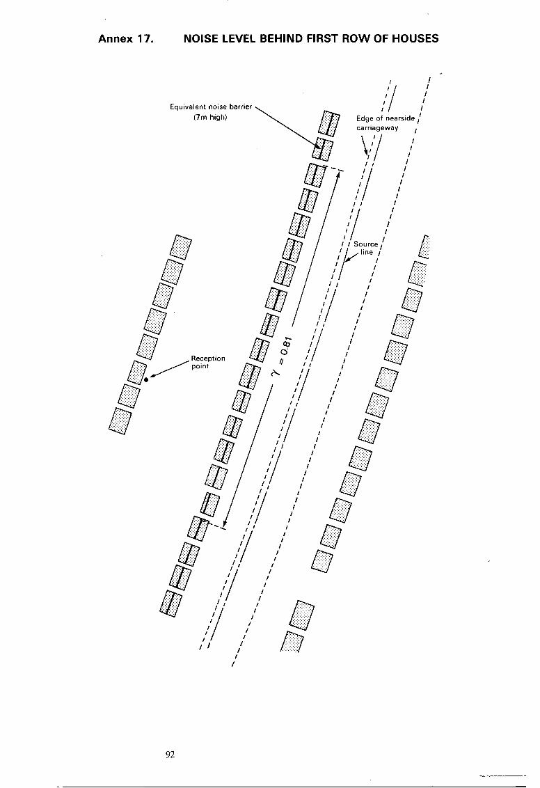
Annex 17. NOISE LEVEL BEHIND FIRST ROW OF HOUSES
I /
92
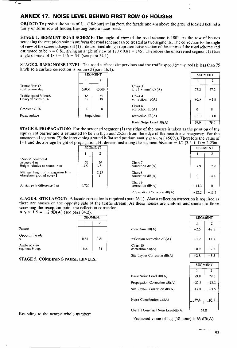
65 19
0
Chart 4 correction dB(A)
Chart 6 correction dB(A)
ANNEX 17. NOISE LEVEL BEHIND FIRST ROW OF HOUSES OBJECT: To predict the value of Llo (18-hour) at l m from the facade and 4m above the ground located behind a fairly uniform row of houses fronting onto a main road.
STAGE 1. SEGMENT ROAD SCHEME: The angle of view of the road scheme is 180". As the row of houses screening the reception point is uniform the road scheme can be treated as two segments. The correction to the angle of view of the screened segment (1) is determined along a representative section of the centre of the road scheme and estimated to be y = 0.81, giving an angle of view of 180 x 0.81 = 146". Therefore the unscreened segment (2) has angle of view of 180 - 146 = 34" (see para 34.1).
STAGE 2. BASIC NOISE LEVEL: The road surface is impervious and the traffic speed (measured) is less than 75 km/h so a surface correction is reauired (Dara 16.1).
\1
SEGMENT I r SEGMENT 7 65000
1 2 Traffic flow Q veh/lS-hour day
Traffic speed V krn/h Heavy vehicles p %
Chart 3 Llo (18-hour) dB(A) 65000
65 19
0
77.2
+2.8
0
-1.0
79.0
Gradient G %
Road surface
Basic Noise Level dB(A) 179.0 STAGE 3. PROPAGATION: For the screened segment (1) the ridge of the houses is taken as the position of the equivalent barrier and is estimated to be 7m high and 25.5m from the edge of the nearside carriageway. For the unscreened segment (2) the intervening ground is flat and predominantly gardens (>90%). Therefore the value of
pagation, H, d :ermined along the segment bisector = 112 (3.5 + 1) = 2.25m. SEGMENT
1=1 and the average height of pi SEGMENT
1 2 2
-7.9
-4.4
0
-12.3
1
-7.9
0
- 14.3
-22.2
Shortest horizontal distance d m Height relative to source h m
Average height of propagation H rn Absorbent ground cover I
79 3.5
0.729
79 3.5
2.25 1
Chart 7 correction dB(A)
Chart 8 correction dB(A)
Chart 9 correction dB(A)
Propagation Correction dB(A)
Barrier path difference 6 rn
STAGE 4. SITE LAYOUT: A facade correction is required (para 26.1). Also a reflection correction is required as there are houses on the opposite side of the traffic stream. As these houses are uniform and similar to those screening the reception point the reflection correction = y x 1:s = 1.2 dB(A)-(see para 34.2).
Facade
I SEGMENT I
correction dB(A)
Opposite facade Y
Angle of view segment 8 deg.
1 0.81 1 0.81 reflection correction dB(A)
Chart 10 correction dB(A)
Site Layout Correction dB(A)
I 146 I 34 -7.2
-3.5 STAGE 5. COMBINING NOISE LEVELS:
I SEGMENT I
Basic Noise Level dB(A)
Propagation Correction dB(A)
Site Layout Correction dB(A) -3.5
Noise Contribution dB(A)
Chart 11 Combined Noise Level dB(A)
Predicted value of Llo (18-hour) is 65 dB(A) Rounding to the nearest whole number:

Annex 18. SCREENING DUE TO A ROAD IN A RETAINED CUT
B = 15m
.. .
. . . Reception point 1 ;VI/ ' 1_ I;;;;;; ;:;I; \r
... ... . . . . . . . . . ... 0 ' / .. .
E
II U
E
II
9 $ 0
3
d = 16m
I4 E = 30m )I N.B. Y 2 W and (x 3 W therefore A, = W = 3.0
(x = 4.8m 13 = 15.0m E = 30.0m Y = 5.5m W = 3.0m er = o o
94
~

ANNEX 18. SCREENING DUE TO A ROAD IN A RETAINED CUT
Propagation Correction dB(A)
OBJECT: To illustrate the procedure for predicting the potential barrier correction and containment effects for a road in a retained cut.
-13.3
STAGE 1. SEGMENT ROAD SCHEME: For the purpose of this example it can be assumed that the section of retained cut subtends an angle of 120" at the reception point. This segment constitutes the total angle of view of the road and is, therefore, the only segment to be considered.
correction dB(A)
STAGE 2. BASIC NOISE LEVEL: The road is subject to a speed limit of 70 mph with an estimated traffic speed of 108 km/h. The road has zero gradient and no correction AV is required. As the traffic speed is greater than 75 km/h and the road surface is impervious, a surface correction is not required.
+2.5
Traffic fl6w Q veh/H-hour day
Traffic speed V km/h Heavy vehicles p %
Gradient G %
Road surface
108 20
0
Impervious
Chart 3 Llo (18-hour) dB(A)
Chart 4 correction dB(A)
Chart 6 correction dB(A)
correction dB(A)
Basic Noise Level dB(A)
STAGE 3. PROPAGATION: Propagation is c,structed by the screening wall of the retained cut. The path difference (8 = SB + BR - SR, see diagram opposite) is calculated and the potential barrier correction is found using Chart 9. The distance correction is found using Chart 7. Shortest horizontal distance d m Height relative to source h m
Chart 7 correction dB(A)
Average height of propagation H m Absorbent ground cover I
Barrier path difference 6 m 0.287
Chart 8 correction dB(A) I o Chart 9
' correction dB(A) -11.6 I I
Farside retaining wall
Facade
120 Angle of view segment 0 deg.
reflection correction dB(A) I +2.9 I Chart 10 correction dB(A)
Site Layout Correction dB(A)
STAGE 5. OVERALL NOISE LEVEL: There is only one road segment which contributes to the overall noise level.
-13.3
Basic Noise Level dB(A)
Propagation Correction dB(A)
Y- i Site Layout Correction dB(A)
Overall Noise Level dB(A) I 69.5 1 Rounding to the nearest whole number:
Predicted value of L1o (18-hour) is 70 dB(A)
95

Printed in the United Kingdom for Her Majesty’s Stationery Office Dd290866 C40 4/88 398 12521


HMSO publications are available from:
HMSO Publications Centre (Mail and telephone orders only) PO Box 276, London, SW8 5DT Telephone orders 01-622 3316 General enquiries 01-211 5656 (queuing system in operation for both numbers)
HMSO Bookshops 49 High Holborn, London, WC1V 6HB 258 Broad Street, Birmingham, B1 2HE 021-643 3740 Southey House, 33 Wine Street, Bristol, BS1 2BQ (0272) 264306 9-21 Princess Street, Manchester, M60 8AS 061-834 7201 80 Chichester Street, Belfast, BT1 4JY (0232) 238451 71 Lothian Road, Edinburgh, E H 3 9AZ 031-228 4181
HMSO’s Accredited Agents (see Yellow Pages)
and through good booksellers
01-211 5656 (Counter service only)
€6.80 net
ISBN 0 11 550847 3


